ICES-2017-142 Using real Earth Albedo and Earth IR Flux ...

47th International Conference on Environmental Systems ICES-2017-142 16-20 July 2017, Charleston, South Carolina

Using real Earth Albedo and Earth IR Flux for Spacecraft Thermal Analysis

Romain Peyrou-Lauga1 ESA, ESTEC, Noordwijk, The Netherlands

For the last twenty years, Earth observation instruments have been providing invaluable data about Earth radiated energy measured from Space with an increased accuracy and a continuous improved Earth surface coverage. NASA’s CERES experiment has been designed to measure both solar-reflected and Earth-emitted radiation from the top of the atmosphere to the Earth's surface. It currently encompasses 3 similar instruments on board of 3 different Earth observation satellites (Terra since 1999, Aqua since 2002 and Suomi-NPP since 2011). CERES measurements provide essential data to improve our understanding of the Earth's total climate system and climate prediction models. But the accumulation of global and daily Earth radiated energy data is also of a great interest for thermal engineers designing and modelling Earth orbiting spacecraft.

Some standards have defined for a long time Earth thermal environment for spacecraft thermal analysis. It’s nevertheless difficult to keep a track of their origins with the passing years and the way various projects have used them seems coherent but with more or less variations.

The objective of this paper is to recreate a link between real observations and Earth environment assumptions used for Earth orbiting spacecraft thermal analysis, by comparing the common Earth albedo and Earth Infrared flux hypotheses with the real measured Earth radiated energy. From such comparison, one should assess if the current hypotheses cover properly the reality or how to quantify the margin potentially contained in these usual assumptions. As an ultimate goal, this paper aims at evaluating if the usual hypotheses need to be updated.

Nomenclature CERES = Clouds and the Earth's Radiant Energy System ESA = European Space Agency IR = InfraRed ISS = International Space Station LEO = Low Earth Orbit LTAN = Local Time at Ascendant Node NASA = National Aeronautics and Space Administration NPP = National Polar-orbiting Partnership SSO = Sun Synchronous Orbit TRMM = Tropical Rainfall Measuring Mission

1 Thermal engineer, TEC-MTT, [email protected].

International Conference on Environmental Systems

2

I. Introduction his paper aims at recreating a link between real observations and assumptions used for spacecraft thermal analysis. It is based on NASA's Clouds and Earth Radiant Energy System (CERES) data. In a first step, these

data are briefly presented and a monthly albedo and Earth temperature map is proposed, mainly as a typical Earth thermal environment for thermal analysis. In a second step, CERES data are processed with a tool currently developed in ESA to calculate the effective albedo and Earth temperature, as viewed from any Earth orbit. These effective albedo / Earth temperature can then be processed to deduced minimum and maximum range that can be applied for thermal analysis, including worst cases of variation of perceived Earth thermal environment.

II. Overview of CERES Albedo and Earth IR data

A. CERES data All the albedo and planetary InfraRed emission data was obtained from NASA's Clouds and Earth Radiant

Energy System (CERES) website. Such data is freely provided and available for any use. It gathers various sets of measurements from several similar CERES instruments which flies onboard several spacecrafts, including NASA's Terra satellite, which is in a polar sun-synchronous orbit with an altitude of 705 km and a descending node of 10:30 am mean local time. The CERES instrument is a radiometer measuring shortwave (0.3 – 5 μm) and thermal (8 – 12 μm) emission from the top of the atmosphere. Data is collected for the whole Earth with coverage at approximately 10:30 am local time every day. The data products available include computed albedo and IR emission.

Data used for this paper was obtained for every day in the five year period 2007-2011 inclusive (1826 days). The product chosen was SYN1deg, which shows the measured data on a 1° by 1° grid covering the entire globe.

Figure 1 shows typical Earth mapping of albedo (on the left) and Earth IR flux from top of the atmosphere (on the right). This latter can also be expressed as an equivalent black body temperature, which is preferably used in this paper. Data illustrated in the Figure 1 corrresponds here to an Equinox day (21/03/2011), a day in the year when all parts of the Earth are Sun illuminated during 12 consecutive hours, which makes albedo measurement from CERES orbit possible for all regions of the Earth. The grid superimposed to the albedo / Earth IR mapping corresponds to CERES grid, which has 1° by 1° granularity.

Figure 1: Measured albedo (on the left) and Earth IR flux from top of the atmosphere (on the right) on Spring Equinox (21/03/2011)

B. CERES albedo data

The albedo data gives the top of atmosphere reflectivity in the range 0 – 1. Figure 2 provides an example of daily data for albedo for the entire Earth surface for a random day in Winter. Some parts of this albedo map appear with missing data. It is indeed not possible to get albedo measurement for the Northern high latitude regions in Winter and for Southern high latitude regions in Summer as these regions remain in the shade part of the year. Besides this seasonal limitation, other small portions of the Earth surface may appear as missing data (2 of them are visible in

T


3

Figure 2) probably because of lack of full Earth coverage from CERES instrument some days or short non operational periods.

Figure 2: Example of daily albedo data (CERES).

C. CERES Earth IR flux data

Unlike albedo measurement, Earth IR flux measurement do not depend on Sun illumination conditions. Therefore the full coverage of the Earth surface is easier whatever the season is and it is not limited by the day/night alternance. Nevertheless some limited portions of Earth surface may seem to escape measurement some days, due to Instrument field of view combined with orbit or due to short non-operational periods. Figure 3 provides an example of daily data for IR flux corresponding to the same day as the previous figure (albedo map).

Figure 3: Example of daily IR data (CERES).

III. 1st Step: Average montly albedo and Earth IR flux CERES data can be directly processed to obtain monthly average albedo depending on latitude and month. Using

5 years of data (from 01/01/2007 to 31/12/2011), the repeatability from a year to another can be checked.


4

A. Albedo Table 1 presents average albedo for each month of the year and for each 10° range of latitude. These data are

based on the compilation of 5 years of albedo measurement (01/01/2007 to 01/01/2012) by CERES instruments. Table 1: Average measured albedo values over 5 years depending on the latitude and depending on the season based on 5 years of CERES albedo measurement (2007-2011)

Average

Latitude Jan Feb Mar Apr May Jun Jul Aug Sep Oct Nov Dec

Ave.

over

2007

Ave.

over

2008

Ave.

over

2009

Ave.

over

2010

Ave.

over

2011

Average

over 5‐

year

85° nan nan 0.64 0.62 0.62 0.57 0.50 0.52 0.58 0.65 nan nan 0.59 0.58 0.59 0.59 0.58 0.59

75° nan 0.66 0.62 0.60 0.58 0.49 0.43 0.44 0.49 0.57 0.65 nan 0.55 0.55 0.55 0.55 0.55 0.55

65° 0.59 0.55 0.53 0.51 0.45 0.38 0.36 0.38 0.42 0.50 0.56 0.59 0.49 0.49 0.48 0.48 0.49 0.49

55° 0.50 0.48 0.44 0.39 0.37 0.35 0.35 0.36 0.37 0.41 0.48 0.51 0.42 0.42 0.42 0.42 0.42 0.42

45° 0.45 0.42 0.38 0.34 0.33 0.32 0.31 0.30 0.30 0.34 0.40 0.45 0.36 0.36 0.36 0.37 0.36 0.36

35° 0.36 0.35 0.32 0.30 0.28 0.27 0.25 0.24 0.26 0.28 0.32 0.36 0.30 0.29 0.30 0.30 0.30 0.30

25° 0.28 0.26 0.25 0.24 0.24 0.24 0.24 0.24 0.24 0.24 0.26 0.28 0.25 0.25 0.25 0.25 0.25 0.25

15° 0.22 0.20 0.20 0.20 0.21 0.23 0.25 0.25 0.25 0.23 0.23 0.23 0.22 0.22 0.22 0.22 0.23 0.22

5° 0.24 0.22 0.22 0.23 0.25 0.26 0.26 0.25 0.25 0.24 0.25 0.25 0.24 0.24 0.24 0.25 0.25 0.24

‐5° 0.24 0.23 0.22 0.22 0.21 0.21 0.21 0.21 0.21 0.22 0.23 0.23 0.22 0.22 0.22 0.22 0.22 0.22

‐15° 0.23 0.23 0.21 0.20 0.20 0.21 0.21 0.21 0.21 0.22 0.23 0.23 0.22 0.21 0.22 0.22 0.22 0.22

‐25° 0.22 0.21 0.22 0.23 0.25 0.26 0.25 0.23 0.23 0.23 0.23 0.23 0.23 0.23 0.23 0.24 0.23 0.23

‐35° 0.24 0.25 0.26 0.29 0.31 0.33 0.32 0.30 0.29 0.27 0.27 0.26 0.28 0.28 0.28 0.28 0.28 0.28

‐45° 0.32 0.33 0.35 0.37 0.40 0.41 0.40 0.37 0.35 0.33 0.33 0.33 0.36 0.36 0.36 0.36 0.36 0.36

‐55° 0.40 0.40 0.42 0.45 0.48 0.51 0.49 0.46 0.44 0.41 0.41 0.40 0.44 0.44 0.44 0.44 0.44 0.44

‐65° 0.49 0.49 0.51 0.55 0.60 0.61 0.64 0.63 0.61 0.59 0.55 0.51 0.56 0.57 0.57 0.57 0.57 0.57

‐75° 0.63 0.64 0.65 0.68 0.74 nan nan 0.73 0.70 0.69 0.66 0.64 0.68 0.67 0.68 0.67 0.67 0.68

‐85° 0.67 0.68 0.69 0.74 nan nan nan nan 0.72 0.70 0.68 0.67 0.69 0.69 0.69 0.69 0.69 0.69

Total 0.32 0.32 0.32 0.31 0.31 0.30 0.30 0.30 0.31 0.31 0.32 0.32 0.31 0.31 0.31 0.31 0.31 0.31

Figure 4 illustrates the previous table.

Figure 4: Illustration of average measured albedo values over 5 years depending on the latitude and depending on the season based on 5 years of CERES albedo measurement (2007-2011)


5

D. Earth IR flux Table 2 presents average Earth IR flux for each month of the year and for each 10° range of latitude. These data

are based on the compilation of 5 years of albedo measurement (01/01/2007 to 01/01/2012) by CERES instruments..

Table 2: Average measured Earth IR flux over 5 years depending on the latitude and depending on the season based on 5 years of CERES Earth IR measurement (2007-2011) (values in W/m2)

Average


Ave.

over

2007

Ave.

over

2008

Ave.

over

2009

Ave.

over

2010

Ave.

over

2011

Average

over 5‐

year

85° 166 W 175 W 173 W 190 W 210 W 226 W 229 W 220 W 205 W 188 W 177 W 171 W 194 W 193 W 194 W 194 W 194 W 194 W









‐5° 241 W 239 W 240 W 244 W 257 W 263 W 264 W 266 W 263 W 257 W 251 W 246 W 253 W 252 W 252 W 253 W 253 W 253 W









Average 236 W 236 W 237 W 238 W 239 W 241 W 243 W 243 W 241 W 239 W 236 W 235 W 239 W 238 W 238 W 239 W 239 W 239 W

Considering Earth as a Black Body, Earth IR flux is converted into equivalent temperature. Table 3 presents equivalent the average Earth temperature for each month of the year as a function of the latitude. Table 3: Average measured Earth black body temperature over 5 years depending on the latitude and depending on the season based on 5 years of CERES Earth IR measurement (2007-2011) (values in K)

Average


Ave.

over

2007

Ave.

over

2008

Ave.

over

2009

Ave.

over

2010

Ave.

over

2011

Average

over 5‐

year

85° 233 236 235 241 247 251 252 250 245 240 236 234 242 242 242 242 242 242

75° 235 236 237 242 248 251 253 251 247 242 238 236 243 243 243 244 243 243

65° 237 238 241 245 249 253 254 252 249 244 240 237 245 245 245 245 245 245

55° 241 242 244 248 251 253 255 254 251 248 244 242 248 248 248 248 248 248

45° 245 246 247 250 253 256 258 259 257 252 249 246 252 252 251 251 252 252

35° 251 251 253 254 257 259 262 262 261 258 255 252 257 257 256 256 256 256

25° 261 261 262 262 262 262 262 262 262 263 262 261 262 262 262 262 262 262

15° 264 265 265 263 261 258 256 255 256 259 261 263 261 261 261 261 260 261

5° 258 259 258 255 254 254 254 255 255 255 256 257 256 255 256 256 256 256

‐5° 255 255 255 256 259 261 261 262 261 260 258 257 258 258 258 258 259 258

‐15° 257 257 259 262 264 265 265 266 265 263 260 258 262 262 262 262 262 262

‐25° 261 262 262 261 261 260 262 262 262 261 260 260 261 261 261 261 261 261

‐35° 260 260 259 257 255 254 254 255 255 256 256 258 257 256 256 257 257 257

‐45° 254 254 253 251 250 249 248 249 249 251 252 253 251 251 251 251 251 251

‐55° 249 249 248 246 245 244 243 243 244 246 247 249 246 246 246 246 246 246

‐65° 247 246 244 241 239 237 237 236 238 241 244 246 242 241 242 241 241 241

‐75° 244 240 235 230 228 225 224 224 226 231 238 243 233 232 233 232 233 233

‐85° 242 236 229 224 222 219 218 216 219 226 235 242 228 228 228 228 228 228

Average 254 254 254 254 255 255 256 256 255 255 254 254 255 255 255 255 255 255

Figure 5 illustrates equivalent the average Earth temperature for each month of the year as a function of the

latitude.


6

Figure 5: Illustration of average measured Earth temperature over 5 years depending on the latitude and depending on the season based on 5 years of CERES Earth IR measurement (2007-2011)

IV. 2nd step: Effective albedo and Earth IR flux perceived from Low Earth orbit

A. A few considerations about Earth field of view from a Low Earth Orbit Before introducing the calculation of

effective albedo/ effective Earth temperature as perceived from a spacecraft, it is useful to consider what is the Earth field of view from a low Earth orbit. Figure 6 illustrates a 2D representation of the Earth field of view from a low Earth orbit (here 800 km altitude), where:

- S is the position of the Spacecraft, - A is the orthogonal projection of the

Spacecraft on the Earth surface, - The angle (and its complementary

angle ) characterises the Earth field of view. The spacecraft sees the Earth as a fragment of a sphere, represented by the arc CC’.

Figure 6: Illustration of effective albedo at a any instant as perceived by an Earth orbiting spaceacraft

The Table 4 below provides the main parameters for typical circular low Earth orbit.


7

Table 4: Earth field of view parameters for several Low Earth circular orbit

Altitude (A-S)

Distance from centre of the Earth (O-S)

Field of view angle (from Earth centre)

Field of view angle (from Spacecraft)

Diameter of part of the Earth viewed by the S/C

(chord C-C’ = 2 x B-C)

Length of maximum arc of viewed part of the Earth

(arc C-C’ = 2 x A-C) 400 km 6 771 km 19.8° 70.2° 4 315 km 4 403 km

600 km 6 971 km 23.9° 66.1° 5 172 km 5 315 km 800 km 7 171 km 27.3° 62.7° 5 848 km 6 071 km

Nota: the distances A-S, O-S, C-C’, B-C refer to Figure 6.

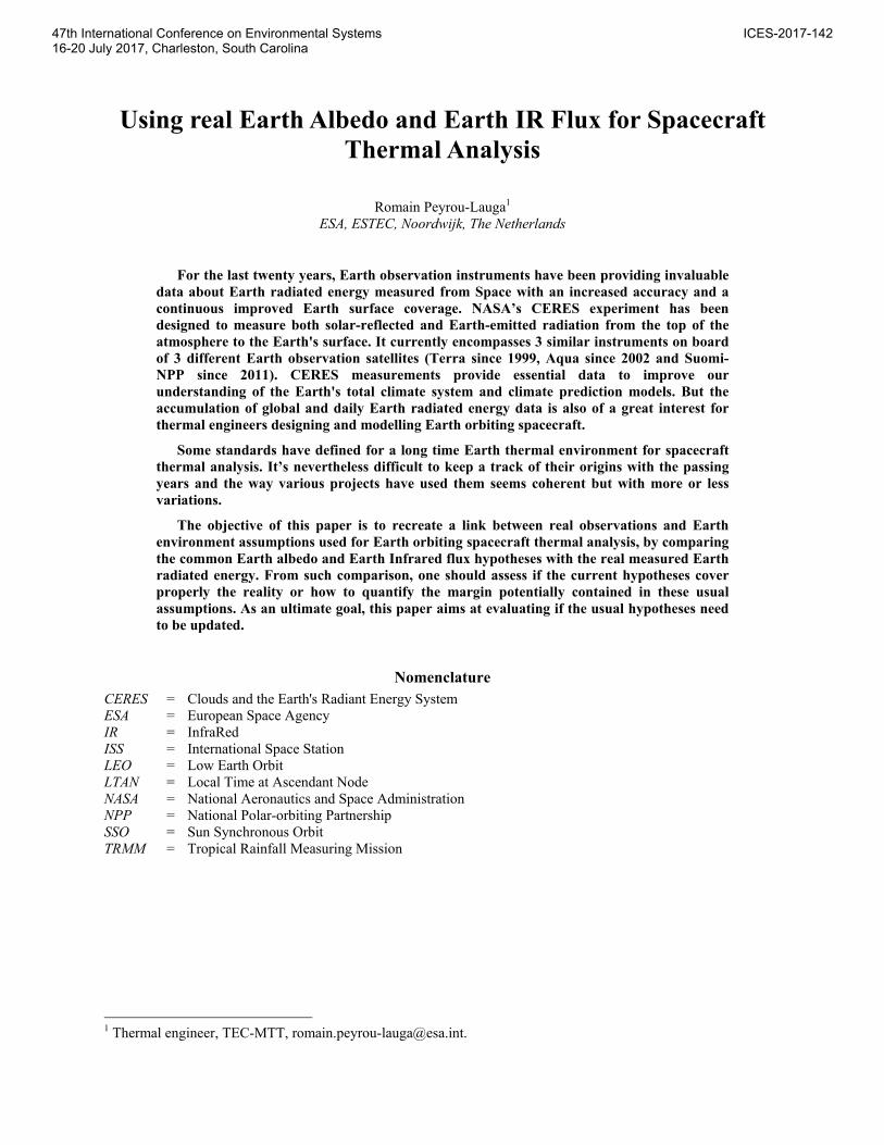
Figure 7 below illustrates how a Spacecraft “sees” the Earth at an altitude of 800km. The total field of view of the Earth from the Spacecraft is represented by the Earth inside the red circle. The meshing of the Earth corresponds to CERES data grid (grid 1° x 1°). At 800 km altitude, the overall field of view of the Spacecraft encompasses about 585 pixels (CERES data elementary surface).

Figure 7: Earth field of view from a spacecraft on a 800 km Low Earth circular orbit

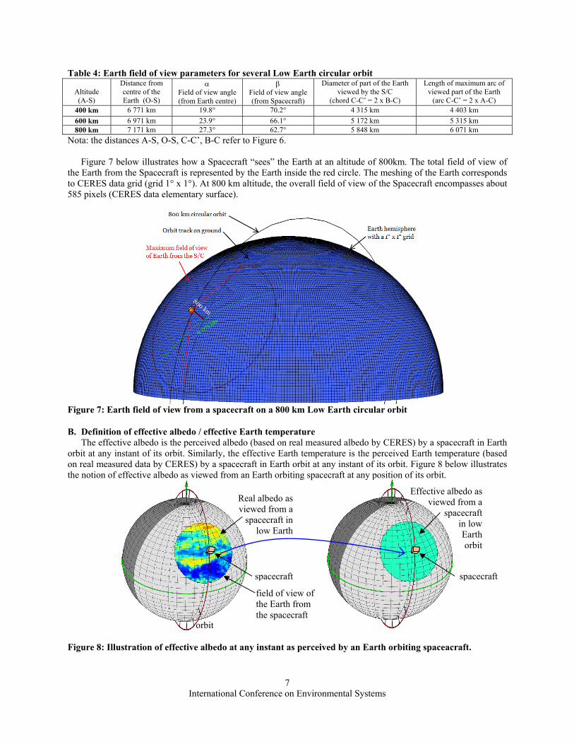
B. Definition of effective albedo / effective Earth temperature The effective albedo is the perceived albedo (based on real measured albedo by CERES) by a spacecraft in Earth

orbit at any instant of its orbit. Similarly, the effective Earth temperature is the perceived Earth temperature (based on real measured data by CERES) by a spacecraft in Earth orbit at any instant of its orbit. Figure 8 below illustrates the notion of effective albedo as viewed from an Earth orbiting spacecraft at any position of its orbit.

Figure 8: Illustration of effective albedo at any instant as perceived by an Earth orbiting spaceacraft.

Real albedo as viewed from a

spacecraft in low Earth

Effective albedo as viewed from a

spacecraft in low Earth orbit

orbit

spacecraft

field of view of the Earth from the spacecraft

spacecraft


8

C. Calculating effective albedo / Earth temperature viewed from any position of any Earth Orbit A tool called OrbEnv is being developed at ESA to process CERES data in order to deduce realistic Earth

environment depending on Spacecraft orbit parameters. It superposes any user defined Earth orbit with CERES albedo and Earth temperature daily map for any day over a large period of time (5 years) processing the combination of: - field of view of each individual visible pixel of CERES albedo/Earth IR flux grid,

- Sun illumination (only used for effective albedo calculation) - spacecraft position on its orbit - spacecraft surface definition (among a limited basic choice, including a plate, sphere or cylinder) - orientation of the surface(s) (among a limited basic choice, including nadir, velocity, antivelocity…etc).

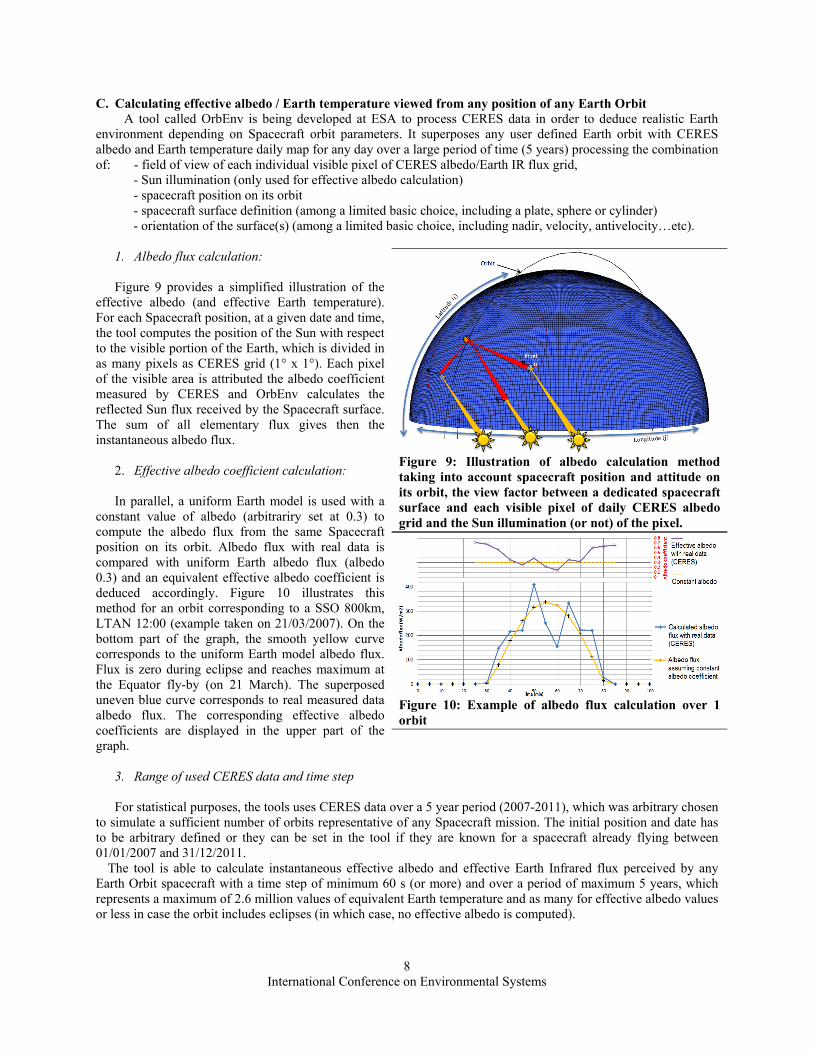
1. Albedo flux calculation: Figure 9 provides a simplified illustration of the

effective albedo (and effective Earth temperature). For each Spacecraft position, at a given date and time, the tool computes the position of the Sun with respect to the visible portion of the Earth, which is divided in as many pixels as CERES grid (1° x 1°). Each pixel of the visible area is attributed the albedo coefficient measured by CERES and OrbEnv calculates the reflected Sun flux received by the Spacecraft surface. The sum of all elementary flux gives then the instantaneous albedo flux.

2. Effective albedo coefficient calculation: In parallel, a uniform Earth model is used with a

constant value of albedo (arbitrariry set at 0.3) to compute the albedo flux from the same Spacecraft position on its orbit. Albedo flux with real data is compared with uniform Earth albedo flux (albedo 0.3) and an equivalent effective albedo coefficient is deduced accordingly. Figure 10 illustrates this method for an orbit corresponding to a SSO 800km, LTAN 12:00 (example taken on 21/03/2007). On the bottom part of the graph, the smooth yellow curve corresponds to the uniform Earth model albedo flux. Flux is zero during eclipse and reaches maximum at the Equator fly-by (on 21 March). The superposed uneven blue curve corresponds to real measured data albedo flux. The corresponding effective albedo coefficients are displayed in the upper part of the graph.

Figure 9: Illustration of albedo calculation method taking into account spacecraft position and attitude on its orbit, the view factor between a dedicated spacecraft surface and each visible pixel of daily CERES albedo grid and the Sun illumination (or not) of the pixel.

Figure 10: Example of albedo flux calculation over 1 orbit

3. Range of used CERES data and time step For statistical purposes, the tools uses CERES data over a 5 year period (2007-2011), which was arbitrary chosen

to simulate a sufficient number of orbits representative of any Spacecraft mission. The initial position and date has to be arbitrary defined or they can be set in the tool if they are known for a spacecraft already flying between 01/01/2007 and 31/12/2011.

The tool is able to calculate instantaneous effective albedo and effective Earth Infrared flux perceived by any Earth Orbit spacecraft with a time step of minimum 60 s (or more) and over a period of maximum 5 years, which represents a maximum of 2.6 million values of equivalent Earth temperature and as many for effective albedo values or less in case the orbit includes eclipses (in which case, no effective albedo is computed).


9

V. Processing effective albedo and Earth temperature

A How to calculate average effective albedo / Earth temperature over a period Instantaneous effective albedo/IR temperature can be easily post-processed to obtain average values over any

duration periods (e.g. over 15 min, over 30 min, over an orbit…). Average Earth temperature over any period is quite straight forward to compute.

Average effective albedo coefficient over a period requires more care: Only average albedo values can be calculated outside eclipse period. And the average value has to be calculated using Sun illumination ratios of each corresponding portion of Earth as weighing factors. It is equivalent to use each albedo flux assuming constant albedo coefficient (as previously described). Figure 11 illustrates the average albedo calculation over a 15 minute’s period using weighting factor.

Figure 11: Illustration of average effective albedo calculation over a period

B Average effective albedo / Earth temperature over an entire orbit 1. Range of orbital average albedo / Earth temperature depending on the orbit

Table 5 presents a synthesis of average effective albedo / Earth temperature over an orbit for several LEO orbits.

- over 5 years (~26 000 orbits) - using real measured data from 2007 to 2011 (CERES mission)

The range of average albedo over an orbit and average Earth temperature over an orbit cover respectively 99% of the cases (> 26 000 orbits). Only a few cases (less than 10) can be found outside these range. These range of average orbital albedo and average orbital Earth temperature are recommended for thermal analysis. Table 5: Synthesis of average effective albedo / Earth temperature over an orbit for several LEO orbits

Type of orbit

Altitude Inclination LTAN Range of average albedo over 1 orbit

Range of average Earth temperature over 1 orbit

SSO

800 km

98.6°

06:00 0.25 – 0.40 246 K – 256 K

12:00 0.25 – 0.40 246 K – 256 K

18:00 0.25 – 0.40 246 K – 256 K

20:00 0.24 – 0.40 246 K – 256 K

21:00 0.25 – 0.40 246 K – 256 K

22:00 0.25 – 0.40 246 K – 256 K

ISS 400 km 51.6° drifting 0.19 – 0.40 250 K – 260 K

Tropical 800 km 20° drifting 0.16 – 0.34 253 K – 264 K

Equatorial 800 km 6° drifting 0.15 – 0.31 253 K – 260 K

There is a noteworthy similarity of results for all Sun-synchronous orbits (SSO) which fly equally over all Earth

latitudes. The less inclined orbits (ISS orbit at 51.6°, “tropical orbit” at 20° and to a larger extend the “equatorial orbit” at

6°) include smaller albedo values, which are typical from equatorial regions (as seen in Table 1 and Figure 4). Tropical and equatorial orbits orbital albedo range is shifted towards lower values as these orbits don’t see the polar regions which feature higher albedo coefficients.

In the same way, orbits with low inclination have a rather high orbital Earth temperature range which is in line with the Earth temperature map, as seen in Table 3 and Figure 5.


10

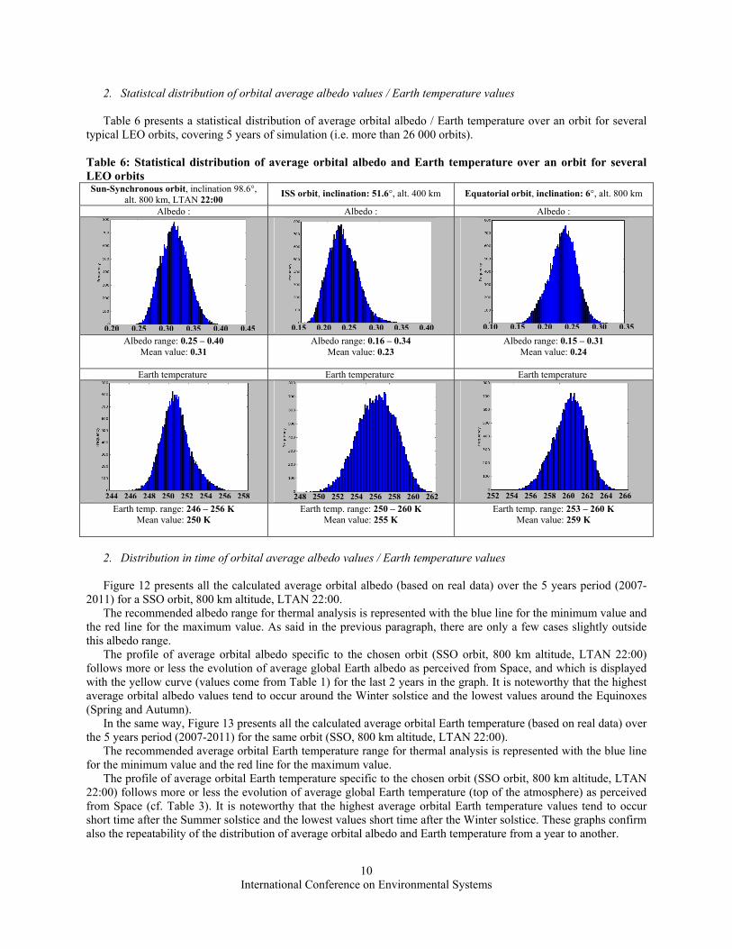
2. Statistcal distribution of orbital average albedo values / Earth temperature values Table 6 presents a statistical distribution of average orbital albedo / Earth temperature over an orbit for several

typical LEO orbits, covering 5 years of simulation (i.e. more than 26 000 orbits).

Table 6: Statistical distribution of average orbital albedo and Earth temperature over an orbit for several LEO orbits Sun-Synchronous orbit, inclination 98.6°,

alt. 800 km, LTAN 22:00 ISS orbit, inclination: 51.6°, alt. 400 km Equatorial orbit, inclination: 6°, alt. 800 km

Albedo : Albedo : Albedo :

Albedo range: 0.25 – 0.40

Mean value: 0.31

Albedo range: 0.16 – 0.34Mean value: 0.23

Albedo range: 0.15 – 0.31Mean value: 0.24

Earth temperature Earth temperature Earth temperature

Earth temp. range: 246 – 256 K

Mean value: 250 K

Earth temp. range: 250 – 260 KMean value: 255 K

Earth temp. range: 253 – 260 K Mean value: 259 K

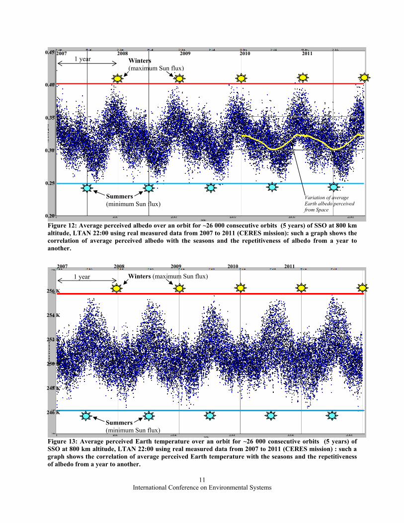
2. Distribution in time of orbital average albedo values / Earth temperature values Figure 12 presents all the calculated average orbital albedo (based on real data) over the 5 years period (2007-

2011) for a SSO orbit, 800 km altitude, LTAN 22:00. The recommended albedo range for thermal analysis is represented with the blue line for the minimum value and

the red line for the maximum value. As said in the previous paragraph, there are only a few cases slightly outside this albedo range.

The profile of average orbital albedo specific to the chosen orbit (SSO orbit, 800 km altitude, LTAN 22:00) follows more or less the evolution of average global Earth albedo as perceived from Space, and which is displayed with the yellow curve (values come from Table 1) for the last 2 years in the graph. It is noteworthy that the highest average orbital albedo values tend to occur around the Winter solstice and the lowest values around the Equinoxes (Spring and Autumn).

In the same way, Figure 13 presents all the calculated average orbital Earth temperature (based on real data) over the 5 years period (2007-2011) for the same orbit (SSO, 800 km altitude, LTAN 22:00).

The recommended average orbital Earth temperature range for thermal analysis is represented with the blue line for the minimum value and the red line for the maximum value.

The profile of average orbital Earth temperature specific to the chosen orbit (SSO orbit, 800 km altitude, LTAN 22:00) follows more or less the evolution of average global Earth temperature (top of the atmosphere) as perceived from Space (cf. Table 3). It is noteworthy that the highest average orbital Earth temperature values tend to occur short time after the Summer solstice and the lowest values short time after the Winter solstice. These graphs confirm also the repeatability of the distribution of average orbital albedo and Earth temperature from a year to another.

0.20 0.25 0.30 0.35 0.40 0.45 0.15 0.20 0.25 0.30 0.35 0.40 0.10 0.15 0.20 0.25 0.30 0.35

244 246 248 250 252 254 256 258 248 250 252 254 256 258 260 262 252 254 256 258 260 262 264 266


11

Figure 12: Average perceived albedo over an orbit for ~26 000 consecutive orbits (5 years) of SSO at 800 km altitude, LTAN 22:00 using real measured data from 2007 to 2011 (CERES mission): such a graph shows the correlation of average perceived albedo with the seasons and the repetitiveness of albedo from a year to another.

Figure 13: Average perceived Earth temperature over an orbit for ~26 000 consecutive orbits (5 years) of SSO at 800 km altitude, LTAN 22:00 using real measured data from 2007 to 2011 (CERES mission) : such a graph shows the correlation of average perceived Earth temperature with the seasons and the repetitiveness of albedo from a year to another.

1 year

1 year Winters (maximum Sun flux)

Summers (minimum Sun flux)

Variation of average Earth albedo perceived from Space

2007 2008 2009 2010 2011 0.45

0.40

0.35

0.30

0.25

0.20

Winters (maximum Sun flux)

Summers (minimum Sun flux)

256 K 254 K 252 K 250 K 248 K 246 K

2007 2008 2009 2010 2011


12

3. Correlation between orbital average effective albedo and effective Earth temperature for an orbit ? The two previous graphs show that both the average orbital effective albedo and the average orbital effective

Earth temperature tend to follow a pattern along the year, with peak values at different period of the year. One can thus wonder if there is a clear correlation between average orbital effective albedo and average orbital effective Earth temperature at every orbit.

Figure 14 presents a plot of simultaneous average orbital effective albedo and average orbital effective Earth temperature (for a same orbit) for a SSO orbit, 800 km altitude, LTAN 20:00 over 5 years (2007-2011). The horizontal lines represent the boundaries for the recommended Earth temperature for thermal analysis. The vertical lines represent the boundaries for the recommended albedo. One can see a tendency that average orbital albedo increases when average orbital Earth temperature decreases and vice-versa. It is clearly visible that there is no orbit found in the 5 year’s period which simultaneously shows: - both maximum albedo possible

value and maximum Earth temperature value

- both minimum albedo possible value and minimum Earth temperature value

Figure 14: Plot of simultaneous average orbital effective albedo and average orbital effective Earth temperature (for a same orbit) for a SSO orbit, 800 km altitude, LTAN 20:00 over 5 years (2007-2011)

Therefore, it is quite conservative to apply boundary conditions cumulating simultaneously:

- maximum Sun flux, maximum albedo and maximum Earth temperature (hot case) - minimum Sun flux, minimum albedo and minimum Earth temperature (cold case)

since they never occur simultaneously, as seen in Figure 12, Figure 13 and Figure 14.

C Average effective albedo / Earth temperature over shorter period than an orbit Instantaneous effective albedo/IR temperature can be post-processed to obtain average values over shorter

periods than an orbit (e.g. over 15 min, over 30 min…) to study the occurrence of large variation of the Earth thermal environment, which can be detrimental for subsystems (as Earth pointed instrumwnt, focal plane radiators…) which require a very stringent temperature stability. An average value is always defined over a certain duration, and the choice of this duration will depend on the subsystem time constant: the lower it is, the more it makes sense to consider short period of variation of effective albedo / effective Earth temperature.

1. What’s the quickest possible change of effective albedo / effective Earth temperature ?

This duration of change of effective albedo / effective Earth temperature depends on the altitude of the orbit. The lower it is, the smaller the field of view of the Earth is, and the easier it is to quickly change completely the scene view from the Spacecraft.

Recommended orbital Earth temperature

range for thermal analysis

Recommended orbital albedo range for thermal analysis


13

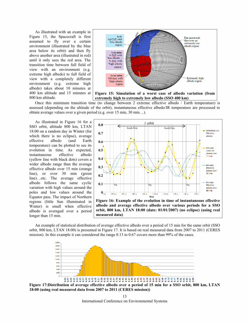
As illustrated with an example in Figure 15, the Spacecraft is first assumed to fly over a certain environment (illustrated by the blue area below its orbit) and then fly above another area (illustrated in red) until it only sees the red area. The transition time between full field of view with an environment (e.g. extreme high albedo) to full field of view with a completely different environment (e.g. extreme high albedo) takes about 10 minutes at 400 km altitude and 15 minutes at 800 km altitude.

Figure 15: Simulation of a worst case of albedo variation (from extremely high to extremely low albedo (SSO 400 km)

Once this minimum transition time (to change between 2 extreme effective albedo / Earth temperature) is assessed (depending on the altitude of the orbit), instantaneous effective albedo/IR temperature are processed to obtain average values over a given period (e.g. over 15 min, 30 min…).

As illustrated in Figure 16 for a SSO orbit, altitude 800 km, LTAN 18:00 on a random day in Winter (for which there is no eclipse), average effective albedo (and Earth temperature) can be plotted to see its evolution in time. As expected, instantaneous effective albedo (yellow line with black dots) covers a wider albedo range than the average effective albedo over 15 min (orange line), or over 30 min (green line)…etc. The average effective albedo follows the same cyclic variation with high values around the poles and low values around the Equator pass. The impact of Northern regions (little Sun illuminated in Winter) is small when effective albedo is averaged over a period longer than 15 min.

Figure 16: Example of the evolution in time of instantaneous effective albedo and average effective albedo over various periods for a SSO orbit, 800 km, LTAN 18:00 (date: 01/01/2007) (no eclipse) (using real measured data)

An example of statistical distribution of average effective albedo over a period of 15 min for the same orbit (SSO

orbit, 800 km, LTAN 18:00) is presented in Figure 17. It is based on real measured data from 2007 to 2011 (CERES mission). In this example it can considered the range 0.13 to 0.67 covers more than 99% of the cases.

Figure 17:Distribution of average effective albedo over a period of 15 min for a SSO orbit, 800 km, LTAN 18:00 (using real measured data from 2007 to 2011 (CERES mission))

Eq.

1 orbit

Eq. Eq.

South Pole North Pole 0.8

0.7

0.6

0.5

0.4

0.3

0.2

0.1

0


14

Taking into account the minimum

and maximum possible values of average effective albedo over a period of 15 min (0.13-0.67 in the previous example), and knowing the minimum possible transition between 2 extreme effective values as established previously (~15 min for a 800 km orbit), a worst case profile of the evolution in time of the average effective albedo (over a period of 15 min) can be defined. It is illustrated in the Figure 18 for the same example (black line, superposed to a random day average effective albedo over 15 min). Figure 18: Worst case profile of the evolution of average effective

albedo over various periods for an SSO orbit, 800 km, LTAN 18:00

VI. Conclusion This work, based on measured Earth albedo and Earth IR flux from CERES, makes now a clear link between real

observations and assumptions used for spacecraft thermal analysis. It can provide useful and realistic inputs to simulate Earth environment, including finding worst cases of thermal conditions changes, which are mainly needed for temperature stability of sensitive instrument or radiators. The OrbEnv tool currently developed in ESA has mainly been used to defined generic albedo / Earth temperature average orbital values, which can be recommended for thermal analysis as shown in the Table 7 below. Table 7: Recommended albedo / Earth temperature over an orbit for the main LEO orbits

Type of orbit

Altitude Inclination LTAN Range of average albedo over 1 orbit

Range of average Earth temperature over 1 orbit

SSO 650 km -850 km ~98-99° any 0.24 – 0.40 246 K – 256 K ISS 400 km 51.6° drifting 0.19 – 0.40 250 K – 260 K

Tropical 800 km 20° drifting 0.16 – 0.34 253 K – 264 K

Equatorial 800 km 6° drifting 0.15 – 0.31 253 K – 260 K

The OrbEnv tool was used in a case by case to define changes of Earth environment, as illustrated in the last

section, and there is some potential to keep developing the tool with a more statistical approach covering a larger range of orbits.

Acknowledgments The author would like to thank Alex Green who built the bases of OrbEnv tool for ESA in 2015.

References CERES CERES SYN1deg Product website: https://ceres.larc.nasa.gov/products.php?product=SYN1deg

Eq.

1 orbit

Eq. Eq.

North Pole South Pole 0.8

0.7

0.6

0.5

0.4

0.3

0.2

0.1

0

ICES-2017-142 Using real Earth Albedo and Earth IR Flux ...

Documents

Transcript of ICES-2017-142 Using real Earth Albedo and Earth IR Flux ...