1 2 3 4 5 6 7 8 91011121314151617181920212223242526272829303132333435363738394041424344454647484950515253545556576061

Development a New Algorithm for Maximum Power Point Tracking of

Partially Shaded Photovoltaic Arrays

Abstract: The photovoltaic (PV) arrays exhibit a nonlinear P-V characteristic and its maximum power point (MPP) varies with solar insolation. Often, the PV arrays get shadowed completely or partially, in which the P-V characteristic get more complex with multi-local MPPs. In this condition most of former methods fails to get global MP. This paper presents a new algorithm to track global MPP under partially shaded condition. The algorithm acts by a heuristic search of array voltage to find global MPP. In the process of heuristic search, reference voltage of PV output is generated and used for perturbation. After each perturbing, results are used for better search, until achieving the convergence constraint. To check the accuracy and precision of the method an accurate model of PV array was implemented in MATLAB software and various tests were conducted.

Keywords: Photovoltaic array, global maximum power

point tracking, partial shading, genetic algorithm

1. Introduction

Tracking the MPP of a PV array is usually an

essential part of a PV system. As such, many MPP

tracking (MPPT) methods have been developed and

implemented. The methods vary in complexity, sensors

required, convergence speed, cost, range of effectiveness,

implementation hardware, popularity, and in other

respects. Among the MPPT methods, the most commonly

known are hill-climbing [1], fractional open-circuit

voltage control [2], perturb and observe (P&O) [3], and

incremental conductance (IncCond) [4]. There are lesser

known, but sometimes very appropriate, methods such as

maximizing load current or voltage [5], fractional short

circuit current control [6], array reconfiguration [7],

linear current control [8], fuzzy control [9], neural

network [10], dc link capacitor droop control [11], and

several others. Only one early example of each technique

was given in the above list, even though we are aware of

more than hundred and seventy papers on different

MPPT techniques, dating from 1968. These techniques

are reviewed and compared in [12].

Mentioned tracking schemes are effective and time

tested under uniform solar insolation, where the P–V

curve of a PV array exhibits only one MPP for a given

temperature and insolation. The occurrence of partially

shaded conditions being quite common (e.g., due to

clouds, trees, etc.) [13], so that there is a need to develop

special MPPT schemes that can track the global MPP

under these conditions.

Some researchers have investigated the global MPPT

of PV systems in the abnormal of temperature and

radiation conditions [14] - [17]. Solodovnik et al. [14]

have presented a state-space-based approach for global

maximum power tracking. This method is fast and

accurate but is system specific, is complex, and requires

more sensors. Miyatake et al. [15] introduce a method

using the Fibonacci sequence to track the maximum value

of global power in the event of partial shading, but the

method does not guarantee tracking the maximum power

for all states of partial shading. Kobayashi et al. [16]

have suggested a two-stage approach to find the global

maximum. In the first stage, the operating point is

transmitted to vicinity of the global maximum point on

the load line pmpmpm IRV = Secondly, the global optimum

point is determined using the IncCond method. pmV and

pmI are estimated to be 80% and 90% of the open-

circuit voltage and short-circuit current, respectively.

This method assumes that the first maximum after

intersection of load line pmpmpm IRV = and the I-V

characteristic of PV system in partial shading mode is

equal with global maximum. However, If the global

maximum point is located in the left of the load line

( actualpm RR > ) then IncCond method in the second stage

of algorithm would not be able to determine the global

maximum.

H. Patel et al. [17] has designed an algorithm based on

the P&O method for global maximum power tracking.

This algorithm uses P&O method to track the maximum

power in uniform insolation. If partial shading occurs,

the critPP ∆>∆ condition is satisfied, and the program

subroutine will be called to determine the global

Hamid Reza Mohajeri*, Mohsen Parsa Moghaddam**, Mahdi Shahparasti***, Mostafa Mohamadian**** * Tarbiat Modares University, hr.mohajeri@modares.ac.ir

** Tarbiat Modares University, parsa@modares.ac.ir

*** Tarbiat Modares University, shahparasti@modares.ac.ir

**** Tarbiat Modares University, mohamadian@modares.ac.ir

489

متلب سایت

MatlabSite.com

MatlabSite.com متلب سایت

1 2 3 4 5 6 7 8 91011121314151617181920212223242526272829303132333435363738394041424344454647484950515253545556576061

maximum. P∆ and critP∆ stand for variation in power

and certain critical power variation values respectively.

The starting point of reference voltage is determined

using flagViVV llastmref ×∆×−= − arg . The refV , lastmV −

and arglV∆ values indicate reference voltage, voltage of

last maximum and disturbance voltage respectively. After

determining the starting point, the P&O method tracks

the local maximum points on PV characteristic one by

one from left to right in P-V curve respectively and stores

them in the memory. The algorithm ends when the first

maximum is tracked in which the maximum power output

is less than the previous maximum.

The performance of this algorithm strongly depends on

the value of arglV∆ , such that if the value of arglV∆ be

considered low, we may lose the global maximum point

while a high value of arglV∆ will increase the

convergence time (in [17] the value of arglV∆ has been

chosen relatively high to avoid the global maximum loss).

The characteristic of P-V in PV system usually has close

peaks in partial shading conditions, so the step-size value

in P&O method should be selected low enough for the

algorithm to be converging. Small step-size reduces the

speed of P&O method and when the algorithm calls the

P&O subroutine several times, reduction in speed is

more easily perceptible. As mentioned in reference [17],

the critPP ∆>∆ condition is checked every 0.1 second to

call the subroutine for tracking global maximum power in

the event of partial shading. It is noteworthy that soiling

(by for example dust) or covering with snow or damage

in some panels in a PV array can occur in the long term

(several weeks or months). While the condition of

critPP ∆>∆ is notable to distinguish this kind of partial

shading, and the algorithm will not operate properly in

that case. This paper presents a new algorithm which

uses a heuristic search for global MPPT in both normal

and partially shaded conditions. In this algorithm there is

no need to determine the time of partial shading, so that

the system don’t make mistake in time of distinguishing

partial shading.

2. Photovoltaic Array Model

One-diode and two-diode models are the models

commonly used for the PV cell. Due to the simplicity,

one-diode model has been more frequently used in

papers, while the two-diode model is much more accurate

and complete. In this paper, the two-diode model

presented in reference [18] is used for PV cell modelling

(see Fig. 1a). The complete data of solar cell and

parameters of double diode model are presented in [18],

so that there aren’t need to repeat.

Fig. 1: (a) Cell equivalent circuit (double diode model) (b) Module

equivalent circuit

By configuring pmsm NN × cells, a module is made (see

Fig. 1b). For electrical modelling of this module, values

of current source and resistors should be multiplied by

pmN and pmsm NN , respectively. If modules are

configured as shown in Fig. 2b, a PV array is made. The

point to be noted in this connection is that the modules

must be parallel with a bypass diode, and in each column

of the PV array a blocking diode should be used. After

using explained circuit model for each module, it can be

shown that the circuit in Fig. 2c is the equivalent circuit

of PV array at uniform insolation. The values of current

source and resistors are the same as values of the PV

module that is multiplied by paN and pasa NN ,

respectively.

PV cell

PV module PV array

Iarrey

Varrey

(a) (b)

Blocking Diodes

Bypass Diodes

Npa =6 and Nsa =5

Npm

D1

ID1a

Rpa Varrey

Iarrey

(c)

Blocking Diode

PV array equivalent circuit

D2

ID2a

Ipha

RsaIpha = IphNpmNpa

ID1a = ID1NpmNpa

ID2a = ID2NpmNpa

Rsa = RsNsmNsa/(NpmNpa)

Rpa = RpNsmNsa/(NpmNpa)

Fig. 2: PV array configuration. (a) PV module. (b) PV array with

bypass and blocking diodes. (c) PV array equivalent circuit

3. Genetic Algorithm

A genetic algorithm (GA) is a procedure used to find

approximate solutions to search problems through

application of the principles of evolutionary biology. The

evolutionary process of a GA is a highly simplified and

stylized simulation of the biological version. It starts from

a population of individuals randomly generated

according to some probability distribution, usually

uniform and updates this population in steps called

generations. Each generation, multiple individuals are

randomly selected from the current population based

upon some application of fitness, bred using crossover,

and modified through mutation to form a new population

[19]. The steps involved in GA are explained as follow:

1. Start: generate random population of i chromosomes

ix (i.e. suitable solution for the problem)

2. Fitness: evaluate the fitness ( )ixf of each

chromosome ix in the population.

3. New population: creating new population by repeating

following steps until the new population is complete.

490

متلب سایت

MatlabSite.com

MatlabSite.com متلب سایت

1 2 3 4 5 6 7 8 91011121314151617181920212223242526272829303132333435363738394041424344454647484950515253545556576061

(3.a) Selection: select two parent chromosomes from a

population according to their fitness (better fitness,

bigger chance to be selected)

(3.b) Crossover: a crossover probability, cross over the

parents to form new offspring. If no crossover was

performed, offspring is the exact copy of parents.

(3.c) Mutation: with a mutation probability, mutate

new offspring at each locus (position in

chromosome)

(3.d) Accepting: place new offspring in the new

population.

Fig. 3: Applying crossover and mutation

4. Replace: use new generated population for a further

run of the algorithm.

5. Test: If the condition is satisfied, stop, and return the

best solution in current population.

6. Loop: go to step2.

The proposed algorithm uses GA process for heuristic

search in MPPT simulation which complete explanation

of that is presented in following.

4. Proposed Algorithm for MPPT

The MPPT problem is a one-dimensional problem in

which the reference voltage ( refV ) for the PV array should

be assigned so that the maximum power can be tracked.

Fig. 4 shows an overview of the circuit used in MATLAB

software for simulation. In this circuit, the PV array has

been modelled according Fig. 2c and connected to a

controllable voltage source. Input reference voltage is

generated by proposed algorithm. By changing in

reference voltage value, the operation point in PV array

changes which causes variation of pvV and pvI . The pvV

and pvI is measured for using in MPPT block.

At the moment t of simulation time, voltage and

output current values of the PV systems, temperature and

radiation are used as input to the MPPT program. Then,

the MPPT program is run one time and gives the

reference voltage refV value to voltage source. The source

sets the PV voltage in refV . MATLAB software simulates

the circuit for next step time.

At ttt ∆+= , MATLAB simulation program calls the

main algorithm. After calling the main program, the

algorithm starts according flowchart of Fig. 5a. In this

algorithm, first the values of temperature, radiation and

changes in output power of PV source (pvP∆ ) are

checked. If there are changes in temperature and

radiation, or in case of partial shading, the output power

will change. In this case, there is a requirement to track

the new maximum power. Therefore, the block3 first

applies the necessary adjustments. If there is no need to a

new MPPT, then block4 checks that MPPT of the

previous call has been converged or not. If last MPPT

converged then the value of reference voltage ( refV ) well

set equal to the global optimum voltage from the previous

MPPT ( bestrefV _ ) else the algorithm should continue. Vpv, Ipv Vref = V

ref-b

est

Data center

Calculation

block

Fig. 4: Circuit used for simulations

Finding of each person’s fitness value by repeating

blocks 7, 8, 9 and 10 until this process is down for all of

persons. In block10, the fitness value of i th person is

calculated and saved. After determining the fitness value

of the i th particle, one unit is added to i . Block11,

checks whether simulations related to all persons have

been performed. If the condition is not true, algorithm

will return to simulation program else it will call new

population subroutine (see Fig. 5b). After establishing

this condition, in fact the step2 of GA algorithm has been

executed, and power output values (or fitness values) for

all the reference voltages (all persons) are obtained.

Block12 implements the steps of 3.a – 3.d in GA

algorithm and returns new population. At this step of

algorithm, the k th replicate of the program is finished.

For the next iteration, block13 checks stop condition of

MPPT. If the condition is not true, the iteration algorithm

begins the )1( +k th repeat, and the MPPT algorithm

reruns according to the mentioned procedure. Iterations

will continue until the convergence condition stops the

MPPT. If the above condition is established, the MPPT

process has been completed and the bestrefV − value will be

the voltage of maximum point.

5. Simulation Results

This section presents the simulation results of two

considered case studies with the proposed algorithm. In

first case study, at first all modules receive normal

insolation and in middle of simulation partial shading

occurs. In second case study, another array configuration

works under partial shading condition and suddenly

pattern of partial shading changes. In following more

explanation is presented.

5.1 Case Study (1)

In this section, a 20×50 modules array is considered.

Under normal circumstances, all panels are subject to

the same temperature and radiation of 2

/1000 mWE =

and CT °= 40 . At st 5.12= , some of the modules

491

متلب سایت

MatlabSite.com

MatlabSite.com متلب سایت

1 2 3 4 5 6 7 8 91011121314151617181920212223242526272829303132333435363738394041424344454647484950515253545556576061

suddenly undergo shading based on the pattern shown in

Fig. 6a. I-V and P-V curves are shown in Fig. 6b for both

uniform insolation and partial shading.

Fig. 5: The flowchart of MPPT algorithm

Simulation results of MPPT for both uniform and

partial shading conditions are shown in Fig. 7a and Fig.

7b. Result curves in Fig. 7a and Fig. 7b are divided into

two parts. In the interval [0 12.5] seconds, the uniform

insolation has been simulated and the rest of the period is

devoted to partial shading condition. As results show, the

algorithm successfully tracked global maximum shown in

Fig. 6b in both normal and partial shading condition.

Radiation and temperature change causes power

changes that lead to starting the MPPT process. A new

heuristic search is started by calling MPPT algorithm. In

initial iterations of the MPPT, value of deviations in

reference voltage is high that is because of random

generation of parents in all range of ][ ocsc VV . In later

iterations deviations become lower by converging to

maximum point. In this case study, MPPT process

completed in 19 and 20 iterations for normal and partial

shading conditions, respectively.

0 50 100 150 200 250 300 350 400 4500

1

2

3

4

5

6

7

x 104

Photovoltaic array volatge(V)

Photo

voltaic

arr

ay c

urr

ent(

A)

and p

ow

er(

W)

Global

maximum

point

P-V curve

under partially

shaded condition

I-V curve

under partially

shaded condition

I-V curve

at normal condition

This fig. shows I*100

P-V curve

at normal

condition

(b)

Fig. 6: Case study (1): (a) partially shaded PV array configuration, (b)

resultant I-V and P-V curves for the explained array

Number of iterations for specific configuration and

condition is not same for different runs. In order to more

illustration, another run has been repeated according to

the mentioned procedure. After re-implementing, the

results of Fig. 7c and Fig. 7d were obtained. The process

of reaching the maximum point in Fig. 7a and Fig. 7c is

quite different. The final value of the reference voltages

for the first and second parts of the simulation in Fig. 7a

are )(08.294 V and )(77.346 V , respectively.

Those values in Fig. 7c are )(13.294 V

and )(78.347 V , respectively. Despite the fact that the

process of reaching the maximum is different in the two

simulations, the final values are the same by little

approximation. The reason of all that is the nature of GA

algorithm is random causing different paths to reach the

optimum point in various runs, but the results for final

reference voltages will be equal with acceptable

approximation.

As simulations and structure of algorithm shows, with

a sudden change in power output of the PV system, the

algorithm is called without having to check whether

partial shading has occurred, while in previous methods

partial shading should first be checked, and in the event

of its occurrence, a separate algorithm should be

implemented. This is main feature of the presented

492

متلب سایت

MatlabSite.com

MatlabSite.com متلب سایت

1 2 3 4 5 6 7 8 91011121314151617181920212223242526272829303132333435363738394041424344454647484950515253545556576061

algorithm that the steps of the maximum power tracking

algorithm are similar for all conditions (normal mode

and partial shading).

0 5 10 15 200

100

200

300

400

500

Voltage a

cro

ss a

rray(V

)

time(s)

0 5 10 15 200

2

4

6

8x 10

4

time(s)

Pow

er

outp

ut

(W)

MPPT starts MPPT starts

shading occursMPP tracked

PART I: normal insolation PART II: partial shading

global MPP tracked

(a)

(b)

0 5 10 15 200

100

200

300

400

Voltage a

cro

ss a

rray(V

)

time(s)

0 5 10 15 20

2

4

6

x 104

time(s)

Pow

er

outp

ut

(W)

global MPP tracked

PART II: partial shadingPART I: normal insolation

(c)

MPPT starts

(d)

shading occurs

MPPT startsMPP tracked

Fig. 7: Simulation results of case study (1) for both uniform and partial shading conditions.

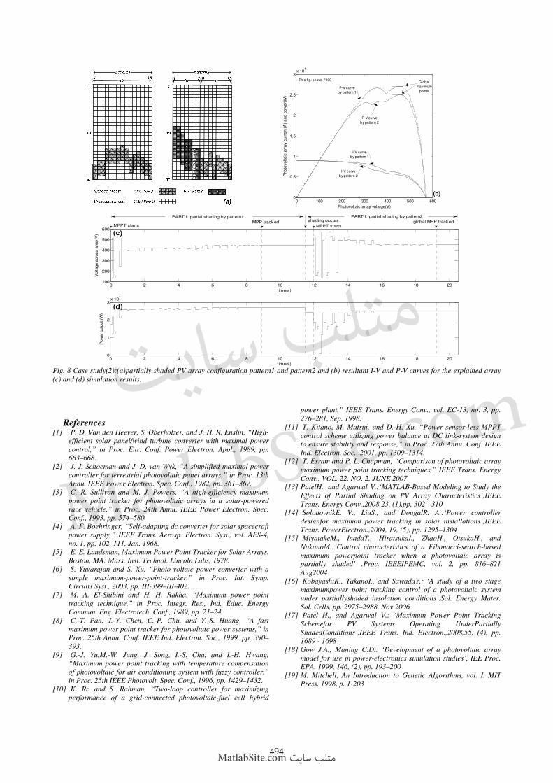
5.2 Case Study (2)

An array some time gets partially shaded which is not

a stable situation. In this condition, pattern of shading

may changes by time. For example, by passing clouds a

dynamic shading may occurs. In this case study, effects of

changing pattern of shading is illustrated. For this

purpose, an array by configuration of Fig. 8a is

considered. At first, partial shading occurs according

pattern1 then in 11.5s the pattern changes to second one.

All data of shading are given in Fig. 8a and P-V and I-V

curves for both patterns are shown in Fig. 8b.

The P-V curve for pattern1 has two peaks which the

voltage of global one is )(5.447 V . The simulation is

tracked exactly at )(63.447 VVref = as global maximum

voltage for pattern1 iterations (Fig. 8c). At 5.11=t , by

changing the pattern according to Fig. 8a the PV output

power changes suddenly and another MPPT process is

started by the algorithm. After 18 iterations,

)(95.454 VVref = is tracked as global maximum point

which accurately coincidence with P-V characteristic of

pattern shown in Fig. 8b. All the explanations and

investigations for the prior case study could be repeated

for this case.

6. Conclusion

This paper presented a new heuristic base algorithm

for MPPT in PV arrays. This algorithm not only has good

performance in uniform insolation but also in terms of

partial shading. Without any complex mathematical

calculation, the global maximum is tracked by using the

intelligence of the GA. The algorithm is simple can be

easily applicable to PV arrays with any kind of

configuration. Determining the exact time of partial

shading is difficult and in some cases impossible. One

feature of the proposed method is that it is called by

changes in PV output power. It means that the tracking

process for normal and partial shading conditions is the

same without any need to understand partial shading

occurrence.

493

متلب سایت

MatlabSite.com

MatlabSite.com متلب سایت

1 2 3 4 5 6 7 8 91011121314151617181920212223242526272829303132333435363738394041424344454647484950515253545556576061

0 100 200 300 400 500 600

0

0.5

1

1.5

2

2.5

3x 10

4

Photovoltaic array volatge(V)

Pho

tovolta

ic a

rray c

urr

ent(

A)

and p

ow

er(

W)

Global

maximum

points

This fig. shows I*100

I-V curve

by pattern 2

I-V curve

by pattern 1

P-V curve

by pattern 2

P-V curve

by pattern 1

(b)

0 2 4 6 8 10 12 14 16 18 20100

200

300

400

500

600

Voltage a

cro

ss a

rray(V

)

time(s)

0 2 4 6 8 10 12 14 16 18 200

1

2

3x 10

4

time(s)

Pow

er outp

ut (W

)

MPPT startsMPPT startsglobal MPP trackedshading occurs

PART I: partial shading by pattern1

MPP tracked

PART I: partial shading by pattern2

(c)

(d)

Fig. 8 Case study(2):(a)partially shaded PV array configuration pattern1 and pattern2 and (b) resultant I-V and P-V curves for the explained array

(c) and (d) simulation results.

References

[1] P. D. Van den Heever, S. Oberholzer, and J. H. R. Enslin, “High-

efficient solar panel/wind turbine converter with maximal power

control,” in Proc. Eur. Conf. Power Electron. Appl., 1989, pp.

663–668.

[2] J. J. Schoeman and J. D. van Wyk, “A simplified maximal power

controller for terrestrial photovoltaic panel arrays,” in Proc. 13th

Annu. IEEE Power Electron. Spec. Conf., 1982, pp. 361–367.

[3] C. R. Sullivan and M. J. Powers, “A high-efficiency maximum

power point tracker for photovoltaic arrays in a solar-powered

race vehicle,” in Proc. 24th Annu. IEEE Power Electron. Spec.

Conf., 1993, pp. 574–580.

[4] A. F. Boehringer, “Self-adapting dc converter for solar spacecraft

power supply,” IEEE Trans. Aerosp. Electron. Syst., vol. AES-4,

no. 1, pp. 102–111, Jan. 1968.

[5] E. E. Landsman, Maximum Power Point Tracker for Solar Arrays.

Boston, MA: Mass. Inst. Technol. Lincoln Labs, 1978.

[6] S. Yuvarajan and S. Xu, “Photo-voltaic power converter with a

simple maximum-power-point-tracker,” in Proc. Int. Symp.

Circuits Syst., 2003, pp. III-399–III-402.

[7] M. A. El-Shibini and H. H. Rakha, “Maximum power point

tracking technique,” in Proc. Integr. Res., Ind. Educ. Energy

Commun. Eng. Electrotech. Conf., 1989, pp. 21–24.

[8] C.-T. Pan, J.-Y. Chen, C.-P. Chu, and Y.-S. Huang, “A fast

maximum power point tracker for photovoltaic power systems,” in

Proc. 25th Annu. Conf. IEEE Ind. Electron. Soc., 1999, pp. 390–

393.

[9] G.-J. Yu,M.-W. Jung, J. Song, I.-S. Cha, and I.-H. Hwang,

“Maximum power point tracking with temperature compensation

of photovoltaic for air conditioning system with fuzzy controller,”

in Proc. 25th IEEE Photovolt. Spec. Conf., 1996, pp. 1429–1432.

[10] K. Ro and S. Rahman, “Two-loop controller for maximizing

performance of a grid-connected photovoltaic-fuel cell hybrid

power plant,” IEEE Trans. Energy Conv., vol. EC-13, no. 3, pp.

276–281, Sep. 1998.

[11] T. Kitano, M. Matsui, and D.-H. Xu, “Power sensor-less MPPT

control scheme utilizing power balance at DC link-system design

to ensure stability and response,” in Proc. 27th Annu. Conf. IEEE

Ind. Electron. Soc., 2001, pp. 1309–1314.

[12] T. Esram and P. L. Chapman, “Comparison of photovoltaic array

maximum power point tracking techniques,” IEEE Trans. Energy

Conv., VOL. 22, NO. 2, JUNE 2007

[13] PatelH., and Agarwal V.:‘MATLAB-Based Modeling to Study the

Effects of Partial Shading on PV Array Characteristics’,IEEE

Trans. Energy Conv.,2008,23, (1),pp. 302 - 310

[14] SolodovnikE. V., LiuS., and DougalR. A.:‘Power controller

designfor maximum power tracking in solar installations’,IEEE

Trans. PowerElectron.,2004, 19, (5), pp. 1295–1304

[15] MiyatakeM., InadaT., HiratsukaI., ZhaoH., OtsukaH., and

NakanoM.:‘Control characteristics of a Fibonacci-search-based

maximum powerpoint tracker when a photovoltaic array is

partially shaded’ .Proc. IEEEIPEMC, vol. 2, pp. 816–821

Aug2004

[16] KobayashiK., TakanoI., and SawadaY.: ‘A study of a two stage

maximumpower point tracking control of a photovoltaic system

under partiallyshaded insolation conditions’.Sol. Energy Mater.

Sol. Cells, pp. 2975–2988, Nov 2006

[17] Patel H., and Agarwal V.: ‘Maximum Power Point Tracking

Schemefor PV Systems Operating UnderPartially

ShadedConditions’,IEEE Trans. Ind. Electron.,2008,55, (4), pp.

1689 - 1698

[18] Gow J.A., Maning C.D.: ‘Development of a photovoltaic array

model for use in power-electronics simulation studies’, IEE Proc.

EPA, 1999, 146, (2), pp. 193–200

[19] M. Mitchell, An Introduction to Genetic Algorithms, vol. I. MIT

Press, 1998, p. 1-203

494

متلب سایت

MatlabSite.com

MatlabSite.com متلب سایت