Ice Slurry as Secondary Fluid in Refrigeration Systems

Fundamentals and Applications in Supermarkets

Licentiate Thesis by Cecilia Hägg

Stockholm, November 2005

School of Industrial Engineering and Management Department of Energy Technology

Division of Applied Thermodynamics and Refrigeration

ii

Ice Slurry as Secondary Fluid in Refrigeration Systems Fundamentals and Applications in Supermarkets Cecilia Hägg

Trita REFR Report No. 05/48 ISSN 1102-0245 ISRN KTH/REFR/R-05/48-SE ISBN 91-7178-192-7

Licentiate Thesis by Cecilia Hägg School of Industrial Engineering and Management Department of Energy Technology Division of Applied Thermodynamics and Refrigeration

Printed by Universitetsservice US AB Stockholm, 2005

© Cecilia Hägg, 2005

iii

Abstract This thesis summarises the work performed within the project known as ICE-COOL at the Royal Institute of Technology (KTH) on low tem-perature applications of ice slurry. The ICE-COOL project is a Euro-pean Community funded project within the 5th Framework Program. The task given to KTH was to find and characterize the best possible aqueous solution with a freezing point of -25 °C applicable for ice slurry with an operating temperature of -35 °C. The circumstances differ for low temperature ice slurry from medium temperature as a result of for example the change in thermo-physical properties due to increased addi-tive concentration and the lower temperature.

Ice slurry is a mixture of fine ice crystals, water and freezing point de-pressant additives. The typical ice crystal size ranges between 0.1 to 1 mm in diameter. The main purpose of using ice slurries is to take advan-tage of the latent heat. More than a few requirements are to be fulfilled by an ideal ice slurry fluid. It should have good thermo-physical proper-ties, high heat transport and transfer abilities, as well as low pressure drop to facilitate small pumping power. The ice content of ice slurry af-fects all the mentioned abilities. Apart from the mentioned factors of the fluid, there are other aspects that have to be taken into consideration such as environmental pollution and toxicity, flammability, material compatibility, corrosion, handling security and cost.

This thesis reports on the experiences accomplished and the initial ex-periments performed on low temperature ice slurry. The thesis also gives the background and fundamentals necessary for a discussion and com-parison of different aqueous fluids suitable for ice slurry in general and for low temperature in particular. In addition to the low temperature ap-plication, the thesis also reports on an initial energy consumption com-parison between using ice slurry and single-phase fluid in supermarkets by means of the simulation program CyberMart developed by Jaime Arias at the Department of Energy Technology at KTH.

iv

v

Acknowledgments First of all I would like to thank my supervisor Per Lundqvist and my advisors Åke Melinder and Joachim Claesson, for their support and help along the way.

Special thanks go to Jaime Arias for all the good discussions and answers on supermarket-related questions! I want to thank all my dear colleagues at the Division of Applied Thermodynamics and Refrigeration at KTH. I am also very grateful to Dorothy Furberg who carefully corrected my English.

The financial support within the project ICE-COOL, a European Com-munity funded project in the 5th Framework, is appreciated.

I also want to thank Benedict Lammerding for helping to perform ex-periments on aqueous solution of ethanol.

And finally, I want to thank my friends, family and Christofer, who en-couraged me every now and then along the way!

vi

1

Table of Contents

1 INTRODUCTION 3 1.1 BACKGROUND 3 1.2 INDIRECT SYSTEM 4 1.3 SECONDARY FLUIDS 6 1.4 CHARACTERISTICS OF SOME FREEZING POINT DEPRESSANT ADDITIVES 6 1.5 ICE SLURRY 7 1.6 OBJECTIVES 9 1.7 REFERENCES 10

2 THEORY AND FUNDAMENTALS OF ICE SLURRY 11 2.1 INTRODUCTION 11 2.2 FREEZING POINT AND ICE CONTENT 13 2.3 DENSITY 17 2.4 ENTHALPY AND APPARENT SPECIFIC HEAT 17 2.5 VISCOSITY AND RHEOLOGY 19 2.6 FLUID FOR LOW TEMPERATURE ICE SLURRY 20 2.7 NOMENCLATURE 23 2.8 REFERENCES 24

3 EXPERIMENTS 27 3.1 EXPERIMENTAL APPARATUS 27 3.2 PRESSURE DROP 29

3.2.1 Experience of Pressure Drop from the Literature 29 3.2.2 The Expected Results from the Initial Pressure Drop Experiments 32 3.2.3 The Initial Pressure Drop Experiments 33 3.2.4 Conclusions of Pressure Drop Measurements 41

3.3 HEAT TRANSFER COEFFICIENT 41 3.3.1 Experience of Measured Heat Transfer Coefficient from the Literature 41 3.3.2 The Expected Results from the Heat Transfer Coefficient Experiments 44 3.3.3 The Initial Heat Transfer Coefficient Experiments 45 3.3.4 Conclusions of Heat Transfer Coefficient Measurements 47

3.4 REFERENCES 49 4 SUPERMARKETS AND SYSTEMS 51

4.1 INTRODUCTION 51 4.2 A TOOL FOR COMPARING DIFFERENT SYSTEM SOLUTIONS 52

2

4.3 ENERGY- SAVING TECHNOLOGIES 52 4.4 ICE SLURRY IN PRACTICE 53 4.5 A COMPARISON BETWEEN SINGLE-PHASE AND ICE SLURRY AS SECONDARY FLUID IN SUPERMARKET 54 4.6 REFERENCES 59

5 DISCUSSION, CONCLUSION AND FUTURE WORK 61 5.1 DISCUSSION 61 5.2 CONCLUSIONS 63 5.3 FUTURE WORK 64

6 SUMMARY OF APPENDED PAPERS 67 6.1 PAPER 1 67 6.2 PAPER 2 68 6.3 PAPER 3 68

APPENDIX A 69

3

1 Introduction

1 . 1 B a c k g r o u n d On an annual basis 20-35% of refrigerant charge was emitted to the at-mosphere in 1980 in developed countries (Fischer, 1991) (AEA, 2003). The Montreal Protocol of 1987, which suggested a phase-out of ozone-depleting CFCs and HCFCs, was signed by a number of countries around the world. To speed up the phase-out schedule, amendments were made to the Montreal Protocol in London, Copenhagen and Vi-enna. HFCs have been used as substituting refrigerants for CFCs and HCFCs, but the disadvantage of HFCs is their high global warming po-tential. In the Kyoto Protocol of 1997, the developed countries commit-ted themselves to reducing their collective emissions of six greenhouse gases by at least 5% by the period 2008-2012. The three most important gases are carbon dioxide (CO2), methane (CH4) and nitrous oxide (N2O). The other three long-lived greenhouse gases are hydrofluorocarbons (HFCs), perfluorocarbons (PFCs), and sulphur hexafluoride (SF6).

A useful tool to measure the impact of a refrigeration or air conditioning system is to estimate its life cycle climate performance (LCCP). LCCP includes all of the warming impacts due to the use of the system through its lifetime. Emissions considered include the carbon dioxide emissions from fossil fuel power plants that generate the power to operate the sys-tem, refrigerant emissions during operation of the system, end-of-life re-frigerant disposal losses, refrigerant losses during transport, and embod-ied energy and trace greenhouse gas emissions from production of the refrigerant.

It has been estimated that refrigeration and air conditioning use ap-proximately 15% of the global production of electricity (IIR, 17th Infor-matory Note, 2003). The emission level including fugitive emissions, ruptures, emissions during service and at end of life are generally very high and the larger the charge, the larger the average emission rate, due to very long pipes, the large number of fittings, valves, and huge emis-sions when ruptures occur.

There are several ways to approach the emission problems from refrig-eration. The four most palpable are:

4

(i) To minimize the charge in the refrigeration system needed to generate a certain refrigerating effect:

(ii) To design systems that are leak-proof:

(iii) To use environmentally benign working fluids such as propane, ammonia or carbon dioxide: or

(iv) To increase the efficiency.

1 . 2 I n d i r e c t S y s t e m Depending on the application, size, and choice of working fluid, com-mercial refrigeration systems have many differences. In supermarkets centralized systems are the most common. A series of compressors and condensers are located in a remote machinery room where they provide a cooling medium to display cabinets and cold storage rooms in other parts of the building. The cooling capacity can vary from 20 kW to more than 1 MW, and the amount of refrigerant can range from 100 to 2000 kg. Centralized systems are commonly direct expansion (DX) in which refrigerant circulates throughout the system.

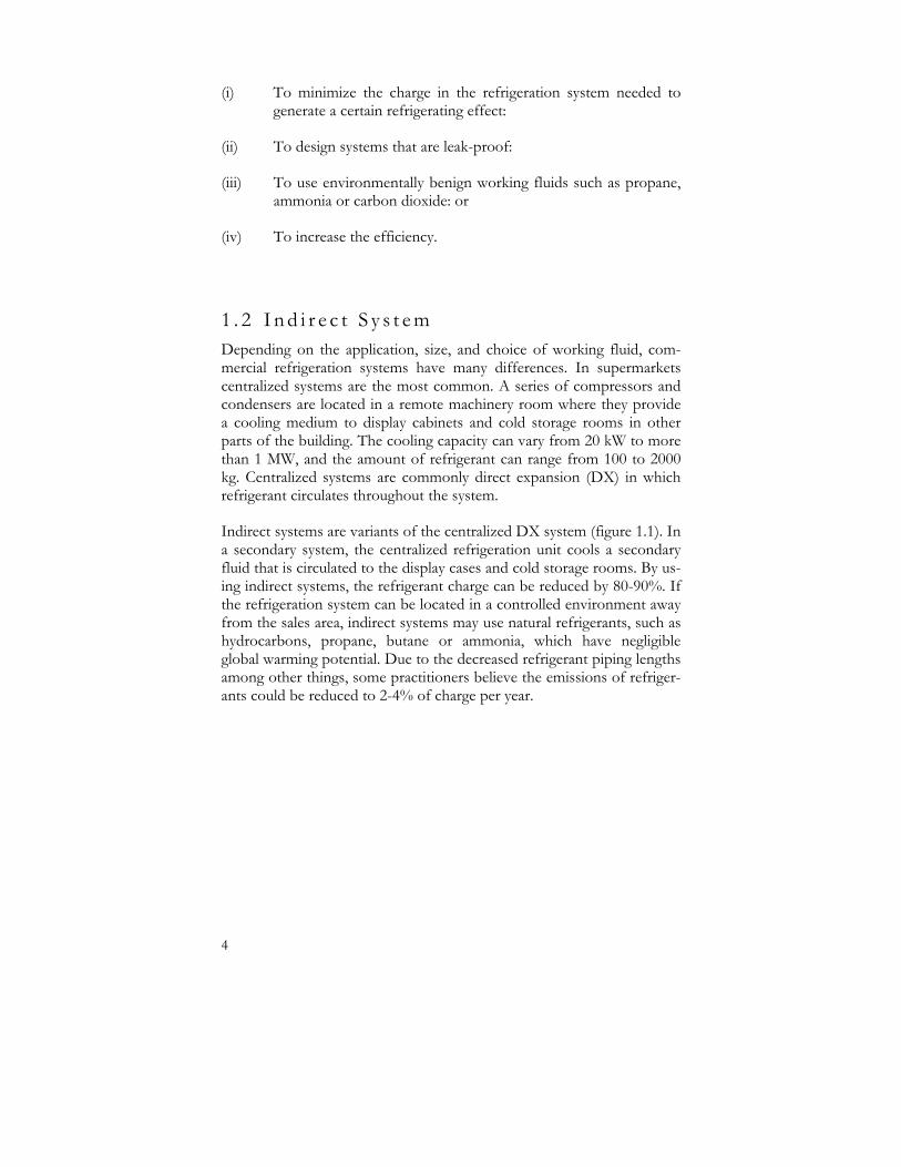
Indirect systems are variants of the centralized DX system (figure 1.1). In a secondary system, the centralized refrigeration unit cools a secondary fluid that is circulated to the display cases and cold storage rooms. By us-ing indirect systems, the refrigerant charge can be reduced by 80-90%. If the refrigeration system can be located in a controlled environment away from the sales area, indirect systems may use natural refrigerants, such as hydrocarbons, propane, butane or ammonia, which have negligible global warming potential. Due to the decreased refrigerant piping lengths among other things, some practitioners believe the emissions of refriger-ants could be reduced to 2-4% of charge per year.

5

F i gu r e 1 .1 Ind i r e c t s y s t em

Secondary systems are the best way to lower emissions from refrigera-tion plants since:

• The charge needed to generate a certain refrigeration ef-fect is reduced in the refrigeration system (i):

• The leakage of refrigerant is reduced by reducing the re-frigerant piping lengths, the number of fittings, valves, but also huge emissions due to ruptures (ii) and

• The use of environmentally benign working fluids is simplified since the refrigeration unit can be located in a controlled room away from the sales area (iii).

Indirect systems, however, contain an extra heat exchanger, which im-plies that indirect systems are more energy consuming than direct expan-sion systems. For indirect refrigeration systems to be competitive with direct expansion systems, they have to be carefully dimensioned. Com-ments on the dimensioning issue for indirect systems have been pub-

Condenser

Compressor Throttle Valve

Heat Exchanger

Heat Load / Utilization

Pump

6

lished in You (2001), Granryd (2002), Lindborg (2003), Verwoerd (1999), Ure (2003) and Arias (2005).

1 . 3 S e c o n d a r y F l u i d s In traditional indirect systems, single-phase secondary fluids based on aqueous solutions have been used. Today there are also other promising technologies with secondary fluids, like two-phase carbon dioxide and ice slurry.

The reason why most preferred single-phase secondary fluids are aque-ous solutions is due to the fact that water has excellent thermo-physical properties. The drawback of pure water is the well known fact that it freezes just below 0 ºC. The most common freezing point depressant additives for water are glycols, alcohols and salts. The choice of additive depends on the application. For freezing (low temperature) application, salts are frequently used. Non-aqueous solutions are also used for low temperature refrigeration.

To keep the energy consumption low, it is important to choose a secon-dary fluid with good heat transport capability, good heat transfer ability and low viscosity, which ensure a small pressure drop and requires low pumping power. To keep the maintenance cost low, it is also important to give attention to corrosion, material compatibility, toxicity and han-dling security (Hägg and Melinder, 2002). There is no ideal secondary fluid for all applications. When choosing a fluid, it is important to find out which parameter is most crucial for the particular application and to choose the best fluid for the current case.

1 . 4 C h a r a c t e r i s t i c s o f S o m e F r e e z i n g P o i n t D e p r e s s a n t A d d i t i v e s

Ethylene glycol is slightly flammable and harmful. The minimum lethal dose is 1-1.5 ml/kg or approximately 100 ml in an adult. Short-term ex-posure can result in irritation to eyes, skin and respiratory tract. Repeated or long-term exposure can bring about effects on the central nervous system and eyes.

Propylene glycol is slightly water-polluting but practically non-toxic to humans. The minimum lethal dose of pure propylene glycol for human adults is more than 15 times greater than with ethylene glycol. Propylene

7

glycol has lower fire hazard when exposed to heat or flame. Propylene glycol can have quite a low pH that might affect the corrosion potential.

Ethyl alcohol is highly flammable and therefore dangerous when ex-posed to heat and flame. Vapours may form explosive mixtures with air. Most vapours are heavier than air. Ethyl alcohol has very low surface tension, which may cause leakage in sealing devices and foaming.

Methyl alcohol is like ethyl alcohol highly flammable. Methyl alcohol is toxic. The chemical is a skin and eye irritant. The substance may be fatal if inhaled, ingested or absorbed through the skin. Ingestion can also cause blindness. The minimum lethal dose for human adults, in absence of medical treatment, is between 0.3 and 1 g/kg.

Methyl alcohol is not compatible with elastomers made of 100% FKM (Viton A), soft rubber or polyether-urethane (EU).

Ammonia causes strong irritation to eyes, skin and the respiratory tract. Swallowing the liquid is corrosive to the mouth, throat and stomach. Exposure to high concentrations can cause temporary blindness and eye damage. Ammonia is highly toxic to aquatic organisms.

Ammonia is not compatible with elastomers made of 100% soft rubber, isoprene (IR), natural rubber (GRS), polyurethane (AU) or silicon rub-bers. Ammonia is not compatible with copper.

This information is based on Merck Chemical Databases, Hazardous Substances Databank (HSB) and Schweitzer (1996).

1 . 5 I c e S l u r r y Ice slurry is a phase-changing secondary fluid consisting of both a liquid-state fraction and a solid–state fraction. The solid-state fraction is com-posed of fine ice particles. The main purpose of using ice slurry is to take advantage of the stored cooling energy in the ice particles when they melt (the latent heat). The ice particles are in the range of 0.1 to 1 mm in diameter. The same aqueous solutions that are used for single-phase sec-ondary fluids are of interest for use as ice slurry.

For single-phase application the working temperature is commonly cho-sen so that the freezing point is in the range of 5-10 ºC below the lowest temperature in the indirect system cycle (figure 1.2). For ice slurry, it is the opposite. It is when the fluid temperature has passed below the

8

freezing point that ice first starts to form, therefore the operating tem-perature is below the freezing point. How much below the freezing point the operating temperature should be is an optimisation issue. The greater the temperature difference is (temperature difference between the freez-ing point and the operating temperature), the greater the ice content. Lower operating temperatures, however, give lower COP of the cooling machine. A lower operating temperature also results in a higher viscosity of the fluid that in turn increases the pressure drop and the required pumping power. Depending on the type of additive and additive concen-tration, the operating temperature for ice slurry can be chosen from 0 to at least -35ºC.

Fi gu r e 1 .2 Op e ra t i n g t empe ra t u r e s v . s . f r e e z i n g p o i n t t empe r a tu r e f o r s i n g l e - p ha s e and i c e s l u r r y

Because of the benefit from the latent heat of the ice, ice slurries have several times higher heat transport capability than single-phase fluids. Due to this and its more complex behaviour, ice slurry is sometimes re-ferred to as an advanced secondary fluid. Ice slurry technology makes it pos-sible to reduce the volume flow rate at a given cooling capacity; this in turn decreases the required pipe dimensions and also allows smaller tem-perature changes over the cooling object, which leads to higher product quality. Beyond the advantages of the traditional indirect systems for lowering the emissions of refrigerants and refrigeration plants, ice slurry is a more efficient secondary fluid than single-phase fluids (iv, see Intro-duction). Using ice slurry with accumulation increases the possibility to

Operating temperature for single-phase secon-dary fluid

Freezing point of the secondary fluid

Operating tempera-ture for ice slurry

T [ºC]

9

build indirect systems without increasing the energy consumption (Chris-tensen, 1998).

This year a handbook1 has been published that summarises the experi-ence and knowledge in ice slurry technology. The handbook treats ice creation, thermo-physical properties of ice slurries, fluid dynamics, ther-modynamics and heat transfer, ice slurry production, transport, stor-ing/melting and mixing, heat exchangers, control systems, optimization, etc. (Kauffeld, Kawaji, Egolf, 2005).

1 . 6 O b j e c t i v e s The objective of this thesis is to summarise the work performed in the project known as ICE-COOL at the Royal Institute of Technology (KTH) on low temperature applications of ice slurry. The ICE-COOL project is a European Community funded project in the 5th Framework Program for research, sub-program for energy, environment and sustain-able development. The ICE-COOL project started in 2002, before this very limited research effort had been put on low temperature ice slurries. The task given to KTH was to find and characterize the best possible secondary fluid for low temperature ice slurry. The circumstances differ for low temperature ice slurry from medium temperature as a result of, for example the change in thermo-physical properties due to increased additive concentration and the lower temperature.

This thesis reports on the experiences gained and the initial experiments performed on low temperature ice slurry. The thesis also gives a back-ground and fundamentals necessary for discussion and comparison of different aqueous fluids suitable for ice slurry in general and for low temperature in particular. In addition to the low temperature application, the thesis also reports on an initial energy consumption comparison be-tween using ice slurry and single-phase fluid in supermarkets by means of the simulation program CyberMart developed by Arias (2005).

1 Handbook on Ice Slurries – Fundamentals and Engineering -

10

1 . 7 R e f e r e n c e s AEA Technology, July 2003. Emissions and Projections of HFCs, PECs and SF6 for the UK and Constituent Countries, report prepared for the Global Atmosphere Division of the UK Department for Environment, Food, and Rural Affairs

Arias, J., 2005. Energy Usage in Supermarkets - Modelling and Field Measure-ments, Doctoral Thesis in Energy Technology, ISBN 91-7178-075-0, Royal Institute of Technology, Stockholm

Christensen, K.G., Kauffeld, M., 1998. Ice Slurry Accumulation, IIR/IIF, sections B and E, Oslo, Norway, June

Fischer, S.K., 1991. Energy and Global Warming Impacts of CFC Alternative Technologies, Alternative Fluorocarbons Environmental Acceptability Study (AFES) and U.S. Department (DOE), Washington, D.C.

Granryd, E., 2002. Optimum Circulation Rates in Indirect Systems, Zero Leak-age – Minimum Charge, IIR/IIF, Stockholm, Sweden

Hägg, C., Melinder, Å., 2002. Selecting Fluids Suitable for Ice Slurry Applica-tions at Low Temperatures, Zero Leakage – Minimum Charge, IIR/IIF, Stockholm, Sweden

IIR, 17th Informatory Note on Refrigerating Technologies, November 2003. How to Improve Energy Efficiency in Refrigerating Equipment

Kauffeld, M., Kawaji, M., Egolf, P.W., 2005. Handbook on Ice Slurries - Fundamentals and Engineering - IIR, ISBN nº 2-913149-42-1

Lindborg, A., 2003. Indirect Refrigeration Systems, 21st Int. Congress of Re-frigeration, IIR/IIF, Washington D.C., USA

Ure, Z., 2003. Secondary Refrigeration European Experiences, ASHRAE Win-ter meeting, Chicago, USA

Verwoerd, M., Liem, N., Gerwen, R..J.M., 1999. Performance of Frozen Food Display Cabinet with Potassium Formate as Secondary Refrigerant, 20th Int. Con-gress of Refrigeration, IIR/IIF, Sydney

You. Y. 2001. Investigation of Deep-freeze Refrigeration Systems in Supermarket Application. Master Thesis at the Dept. of Energy Technology, Royal In-stitute of Technology, Stockholm, Sweden, Royal Institute of Technol-ogy. 92pages

11

2 Theory and Fundamentals of Ice Slur ry

2 . 1 I n t r o d u c t i o n Ice slurry is a mixture of fine ice crystals, water and freezing point de-pressant additives. The typical ice crystal size ranges between 0.1 to 1 mm in diameter. The size depends on additive type and concentration, and the type of ice generator. Without any freezing point depressing ad-ditive, the ice crystal size is typically larger than 1 mm in diameter (E. Stamatiou and M. Kawaji, 2005). The main purpose of using ice slurries is to take advantage of the latent heat. From an economical point of view, ice slurry is pumpable up to an ice fraction of about 30%. More than a few requirements are to be fulfilled by an ideal ice slurry fluid. It should have good thermo-physical properties, high heat transport and transfer abilities as well as low pressure drop to facilitate small pumping power. The ice content of ice slurry affects all the mentioned qualities. Apart from the mentioned factors of the fluid, there are other aspects that have to be taken into consideration, such as environmental pollution and toxicity, flammability, material compatibility, corrosion, handling se-curity and cost.

The concept of “an additive” has already been used in this thesis. Addi-tives used with ice slurry can have different purposes. Additives can be used for lowering the freezing point, preventing the ice particles from agglomerating, to lowering the viscosity, preventing corrosion, etc. The chemical substances of these additives for the various purposes are not the same. In this thesis, the additives are used to lower the freezing point. So far, no work by the author has been performed on other types of additives.

Aqueous fluids have long been used as single-phase fluids in indirect sys-tems. The most commonly used freezing depressant additives are alco-hols, glycols and salts. These fluids can also be used for ice slurry appli-cations. Water itself has excellent thermo-physical properties. The chemicals added to lower the freezing point affect the thermo-physical

12

properties in an unfavourable way. The properties of interest of a single-phase secondary fluid are freezing point, density, viscosity, specific heat and thermal conductivity. For ice slurry the ice concentration need to be determined and instead of specific heat the enthalpy change is of impor-tance. In the general work performed on ice slurry it is assumed that it is pure water that freeze out when the temperature of the fluid pass below the freezing point. Mewisse (2004) writes:

This assumption is valid for diluted solutions, for low to moderate ice formation rates and also the eutectic point of the solution should be at relatively high concentration and low temperature.

Since ice slurry consists of a solid and a liquid phase it is difficult to measure the thermo-physical properties with a desired accuracy. For ice slurry, there is often a density difference between the two phases that contributes to the difficulties in measuring the thermo-physical proper-ties. When measurements are performed with two fractions, it is difficult to get the same conditions each time, which implies that it is very diffi-cult to obtain repeatable measurements.

Many authors have discussed the behaviour of ice slurry, if and when it behaves as a Newtonian fluid or non-Newtonian fluid2 [Guilpart (1999), Egolf a (1999), Stutz (2000), Hansen (2000), Frei (2000), Sari (2000), Doetsch (2002), Kitanovski (2000), Kitanovski (2001)]. Several experi-ments show that ice slurry behaves as a Newtonian fluid at low ice con-centrations, and as a non-Newtonian fluid at high ice concentrations. Even though the behaviour changes with ice content and distribution, it is interesting to make comparisons between aqueous fluids by means of correlations recommended for Newtonian fluids. Another phenomenon that affects how well the estimations will agree with reality is the aging of the ice particles. The shape and size of the ice particles change with time and this change affects the thermo-physical properties [Frei (2000), Pronk (2002), Sari (2000), Egolf (2002), Kitanovski (2001), Van Der Gun (2001), Pronk (2005)].

The basic thermo-physical properties in the following sections have been obtained from Melinder (1997).

2 See section 2.5 Viscosity and Rheology for an explanation of non-Newtonian fluid

13

2 . 2 F r e e z i n g P o i n t a n d I c e C o n t e n t When water freezes out after the temperature of the fluid has passed be-low the freezing point, the concentration of the additive increases in the liquid-phase. The increased additive concentration implies that the freez-ing point of the remaining liquid-phase is further lowered and in order to freeze out more ice the temperature of the fluid has to be further low-ered below the current freezing point of the liquid. The result is that the fluid has no definitive freezing point but rather a freezing range. By plot-ting the freezing point as a function of the additive concentration, one obtains a freezing point curve. Figure 2.1a shows the freezing point curve as a function of the additive mass concentration of different freez-ing point depressants. The lowering of the temperature of the ice slurry is independent of the effect of the latent heat from the phase change, but dependent on the sensible heat of the fluid. Since it is the advantage of the latent heat in ice slurry that is desired, one desires a fluid where the latent heat dominates. To minimise the influence of the sensible heat, a fluid with a relatively low first derivative of the freezing point curve (flat freezing point curve) is to be preferred, see figures 2.1a-b. The first de-rivative of the freezing point curve can be expressed as in equation 2.1

,dcd

A

0ϑ (eq. 2.1)

where ϑ0 is the freezing point temperature and Ac is the additive con-centration giving the freezing point

The ice mass concentration or mass fraction can easily be calculated from equation 2.2 that is based on a mass balance of the additive (see appendix A). Here ( )0ϑc is the initial additive concentration giving the freezing point and ( )ϑAc is the additive concentration of the concen-trated solution (remaining liquid). This equation shows that the ice con-centration is closely linked to the derivative (the slope) of the freezing point curve between the considered temperatures, see figure 2.1a-b.

( ) ( )( )( )

.c

cccA

Ai ϑ

ϑ−ϑ= 0 (eq. 2.2)

14

Figure 2.1a shows the freezing point curve and the concentration of dif-ferent freezing point depressants. The first derivative of the curves de-termines the efficiency of the different additives. The final ice concentra-tion for the aqueous solution is dependant on the additive concentration of the fluid at the original freezing point and its additive concentration in liquid phase at the current temperature below the original freezing point. If the freezing point curves of different depressants have the same de-rivative at the same freezing point, the most efficient fluid is the one with the lowest concentration of additives, see figure 2.1b and figure 2.2a-b. Apart from this, the lower additive concentration is beneficial in the sense that the additives affect the thermo-physical properties unfa-vourably.

-40-38-36-34-32-30-28-26-24-22-20-18-16-14-12-10

-8-6-4-20

0 10 20 30 40 50 60 70Additive Concentraton [%wt]

Free

zing

Poi

nt [º

C]

Potassium formate Potassium acetateCalcium chloride Potassium carbonateAmmonia GlycerolMethyl alcohol Ethyl alcoholPropylene glycol Ethylene glycol

Fi gu r e 2 .1a Fr e e z i n g p o i n t c u r v e o f c ommon f r e e z i n g d e p r e s s an t s

15

-3

-2.5

-2

-1.5

-1

-0.5

0

-30 -25 -20 -15 -10 -5 0Freezing Point [ºC]

Firs

t Der

ivat

ive

of F

reez

ing

Poin

t Cur

ve

Potassium formate Potassium acetateCalcium chloride Potassium carbonateAmmonia GlycerolMethyl alcohol Ethyl alcoholPropylene glycol Ethylene glycol

Fi gu r e 2 .1b Add i t i v e s and t h e d e r i v a t i v e o f t h e f r e e z in g c u r v e w i t h r e f e r e n c e t o f r e e z i n g p o in t

For a fluid with an original freezing point of -25 ºC, a rather large tem-perature difference between the operating temperature and freezing point is needed to obtain a certain ice content in comparison to fluids with an original freezing point of -5 ºC, see figure 2.2a-b. Note the high ice concentration of ethyl alcohol in figure 2.2b, which is due to the de-rivative of the freezing point curve of the ethyl alcohol aqueous solution for freezing point temperatures below –20 °C. Apart from the alcohols and ammonia, potassium formate has the highest ice concentration of the fluids for both temperatures.

16

Ice Fraction at -5 degrees

0

0.05

0.1

0.15

0.2

0.25

0.3

0.35

0.4

0.45

0.5

-10 -9 -8 -7 -6 -5

Temperature [ºC]

Ice

Frac

tion

Potassium formatePotassium acetatePotassium carbonateAmmoniaMethyl alcoholEthyl alcoholPropylene glycolEthylene glycol

Fi gu r e 2 .2a I c e mas s f r a c t i on f o r c ommon f r e e z i n g d e -p r e s s an t a dd i t i v e s f o r f r e e z i n g p o in t - 5 °C

Ice Fraction at -25 degrees

0

0.05

0.1

0.15

0.2

0.25

0.3

0.35

-40 -38 -36 -34 -32 -30 -28 -26

Temperature [ºC]

Ice

Frac

tion

Potassium formatePotassium acetatePotassium carbonateAmmoniaMethyl alcoholEthyl alcoholPropylene glycolEthylene glycol

Fi gu r e 2 .2b I c e mas s f r a c t i on f o r c ommon f r e e z i n g d e -p r e s s an t a dd i t i v e s f o r f r e e z i n g p o in t - 25 °C

17

2 . 3 D e n s i t y Fluid density has a great impact on heat and mass transport capability. In comparison to single-phase fluids, density has an additional impact on the ice slurry. Since ice slurry contains ice with a density lower than the liquid phase, the density difference gives a buoyancy force to the ice par-ticles. As a result of this phenomenon, the density difference causes stratification of the fluid in the pipes and in the storage tank. To prevent stratification in the tank, an agitating system is required and in the pipes, the velocity has to be high enough to avoid a stationary bed. The prob-lem is more significant with ice slurry for low temperature applications than for medium temperature applications since the lower freezing point requires a higher concentration of additives, which increases the density difference between the liquid-phase and the ice particles, except for al-cohols and ammonia.

The density of ice slurry can be derived as follows in equation 2.3:

,)c(c...ccc

mmmm

VVVm

Vm

cf

i

i

i

A

A

w

w

i

i

A

A

w

w

i

iAwi

ρ−

+ρ

==

ρ+

ρ+

ρ

=

=

ρ+

ρ+

ρ

=++

==ρ

111

where ρ is the density, m is the mass, V is the volume, c is the additive concentration, and the indexes i, w, A and cf stand for ice, water, additive and carrier fluid respectively.

2 . 4 E n t h a l p y a n d A p p a r e n t S p e c i f i c H e a t One of the most important properties for dimensioning an ice slurry sys-tem is the enthalpy difference, ∆his Enthalpy difference includes both sensible heat and latent heat of melting. With the aim of estimating en-thalpy values of ice slurry, specific heat, cp, enthalpy of ice, hi, and heat of mixing, ∆hM, of the current solution are of importance. Some additives like alcohols cause an exothermic reaction when they are added to the water and this leads to a volume contraction; this exothermic reaction is

(eq. 2.3)

18

defined as heat of mixing. The enthalpy of ice slurry, his, can be expressed as follows in equation 2.4:

( ) ( )( ),c·,chc·hh icfcfiiis −ϑ+ϑ= 1 (eq. 2.4)

where ci is the ice concentration, hi is enthalpy of ice and hcf is the en-thalpy of the concentrated solution. The enthalpy of the concentrated solution is given from:

( ) ( ) ( )∫ ϑ+ϑ∆+=ϑϑ

ϑ

cf,

R,pcfMR,wcfcf .d·c,chh,ch (eq. 2.5)

In equation 2.5, ccf is the concentration of the carrier fluid, hw,R is the en-thalpy of water at reference temperature; at 0 ºC the enthalpy is 0 kJ/kg. The enthalpy of ice is expressed in equation 2.6, where the heat of the melting of ice is 332.4 kJ/kg (CRC of Handbook of Chemistry and Phys-ics, 1989), (equation 2.4 to 2.6 are based on Melinder, 2002).

( ) ( ).·..·.hi ϑ+ϑ+−=ϑ 00801224332 (eq. 2.6)

The heat capacity for ice slurry includes both sensible heat and latent heat and because of this, it can be referred to as an apparent heat capacity. The apparent heat capacity, cp,is, can be expressed as in equation 2.7:

.hc isis,p ⎟

⎠⎞

⎜⎝⎛

ϑ∂∂

= (eq. 2.7)

19

The apparent heat capacity is directly proportional to the slope of the freezing curve. As has already been discussed in this chapter a flat freez-ing curve yields a high apparent heat capacity due to the fact that phase change is relatively more important than sensible heat.

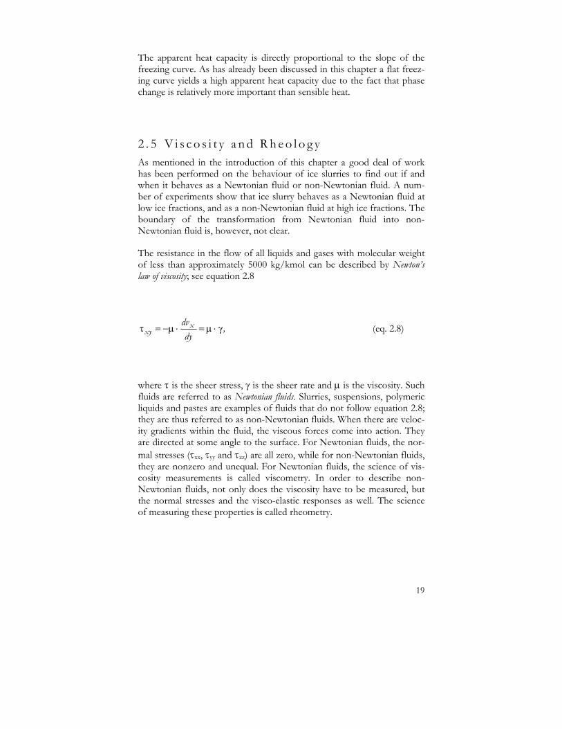
2 . 5 V i s c o s i t y a n d R h e o l o g y As mentioned in the introduction of this chapter a good deal of work has been performed on the behaviour of ice slurries to find out if and when it behaves as a Newtonian fluid or non-Newtonian fluid. A num-ber of experiments show that ice slurry behaves as a Newtonian fluid at low ice fractions, and as a non-Newtonian fluid at high ice fractions. The boundary of the transformation from Newtonian fluid into non-Newtonian fluid is, however, not clear.

The resistance in the flow of all liquids and gases with molecular weight of less than approximately 5000 kg/kmol can be described by Newton’s law of viscosity; see equation 2.8

,dy

dvxxy γ⋅µ=⋅µ−=τ (eq. 2.8)

where τ is the sheer stress, γ is the sheer rate and µ is the viscosity. Such fluids are referred to as Newtonian fluids. Slurries, suspensions, polymeric liquids and pastes are examples of fluids that do not follow equation 2.8; they are thus referred to as non-Newtonian fluids. When there are veloc-ity gradients within the fluid, the viscous forces come into action. They are directed at some angle to the surface. For Newtonian fluids, the nor-mal stresses (τxx, τyy and τzz) are all zero, while for non-Newtonian fluids, they are nonzero and unequal. For Newtonian fluids, the science of vis-cosity measurements is called viscometry. In order to describe non-Newtonian fluids, not only does the viscosity have to be measured, but the normal stresses and the visco-elastic responses as well. The science of measuring these properties is called rheometry.

20

Thomas (1965) introduced an empirical model for calculating the dy-namic viscosity of a Newtonian suspension3; see equation 2.9. This equa-tion takes both the concentration of the solid phase and the interaction between the particles into consideration. The parameters in the model are the viscosity of the liquid phase, µcf, and the ice volume fraction, ci,vol. Thomas writes that the model is valid for particle concentration up to 62.5% and with a particle size ranging from 0.1 to 435 µm. The dynamic viscosity of ice slurry, µis, can then be expressed as

( ),e.c.c. vol,ic.vol,ivol,icfis

⋅⋅+⋅+⋅+µ=µ 6162 0027300510521 (eq. 2.9)

where ci,vol is the volumetric ice fraction (volumetric ice concentration)

.)c(c

cc

cf

iii

ivol,i

ρρ

⋅−+=

1 (eq. 2.10)

Since ice slurry does not always behave as a Newtonian fluid, different types of rheology have been proposed, such as pseudo-plastic and Bing-ham. Another way to obtain viscosity data is from pressure drop meas-urements in pipes. Pressure drop measurements in pipes are discussed in chapter 3.

2 . 6 F l u i d f o r L o w T e m p e r a t u r e I c e S l u r r y In the ICE-COOL project, the task of KTH was to find a suitable aque-ous solution for ice slurry at -35 ºC with a freezing point of -25 ºC. Paper 3 summarizes the work performed at KTH, and the recommended aque-ous solution was the commercial fluid HYCOOL. The final choice of fluid was made by the consortium of ICE-COOL. The decision is based

3 Two-phase fluids with solid particles

21

on experimental work and a theoretical comparison of the thermo-physical properties for common aqueous solutions used as single-phase secondary fluids: ethylene glycol, propylene glycol, ethyl alcohol, methyl alcohol, ammonia, calcium chloride, potassium formate, potassium ace-tate and potassium carbonate. Environmental pollution, toxicity, flam-mability, material compatibility and corrosion aspects were also consid-ered. In the project, the stated criteria of the fluid were:

• Thermal properties: low viscosity, high ability to transport energy by at least 20% of ice at -35 ºC with a freezing point of -25 ºC:

• General characteristics: pH: 7-9.5:

• Environmental impact: non toxic:

• Material compatibility: chemically stable, non corrosive, compatible with iron, copper, aluminium and polymers:

• Price: less than 1.5 € per 1 kg.

In the theoretical comparison, it was found that none of the fluids, ex-cept ethyl and methyl alcohol, could provide an ice fraction higher than 20% at the given freezing point and temperature range. Ammonia gave slightly less than 20% and potassium formate about 17%. The demon-stration ice slurry system that was going to be constructed for ice slurry operating at -35 ºC within the EC project could not be guaranteed to be air tight, which excluded ammonia. Ethyl and methyl alcohol were also excluded since ethanol is very viscous at low temperature and flammable, and methyl alcohol is poisonous at low doses. The best candidate was potassium formate. To speed up the work in the project, the consortium wanted to go for a commercial product. Different commercial products were compared and the final three candidates were HYCOOL, Temper and Freezium, which are manufactured by Norsk Hydro, Temper Tech-nology AB and Kemira respectively. HYCOOL and Freezium are aque-ous fluids based on potassium formate, and Temper is an aqueous fluid based on a mixture of potassium formate and potassium acetate.

A comparison between HYCOOL, Temper and Freezium can be sum-marised as follows:

• Viscosity: Product data from the producers and estimations by means of the Thomas equation show that Temper has higher dynamic vis-cosity than HYCOOL at the current freezing point. Product data and the Thomas equation revealed about 60 mPas for Temper and 27 mPas for HYCOOL at -35 ºC, which is about the same as for Freezium.

22

• Apparent specific heat: Measurements indicate 20% higher values for HYCOOL than for Temper.

• Thermal conductivity: Temper seems to provide slightly higher thermal conductivity values than HYCOOL.

• Homogenety: In comparison with ethanol-based aqueous solutions, both HYCOOL and Temper provide poor homogeneity in a storage tank. The poor homogeneity results from the large density difference between the liquid and the ice. Temper may have a slightly better ability to remain homogeneous than HYCOOL because of its somewhat lower density. HYCOOL and Temper require signifi-cantly better agitator devices to keep the fluid homogeneous in the tank than do ice slurries based on ethanol as an additive.

• Deposited “grey” substances: After running the fluid for some time in the test rig, both HYCOOL and Temper deposited a grey substance. Hydro and Temper technology (manufacturer of HYCOOL and Temper) say they have noticed the problem before and that it is one of the two inhibitors that cause some of the precipitate. The main precipitate probably comes from the inside of the pipe work and from the bottom disc surface of the ice generator, which is brushed to remove the ice.

From among the three commercial fluids, the consortium decided to re-commend HYCOOL.

23

2 . 7 N o m e n c l a t u r e Standard c concentration (mass %) cp specific heat (kJ/kg⋅K) h enthalpy (kJ/kg) ∆h enthalpy difference (kJ/kg) m mass (kg) V volume (m3) v velocity (m/s) ∆hM heat of mixing (kJ/kg)

Greek γ sheer rate (s-1) µ dynamic viscosity (Pa⋅s) ρ density (kg/m3) ϑ temperature (°C) τ sheer stress (Pa)

Subscript A additive i ice w water x x-direction y y-direction z z-direction cf carrier fluid tot total 0 just above the melting region is ice slurry R reference vol volume

24

2 . 8 R e f e r e n c e s CRC Hanbook of Chemistry and Physics, 67th edition, 1989

Doetsch, C., 2002. Pressure Drop Calculation of Ice Slurries Using the Casson model, 5th Ice Slurry Workshop, IIR, Stockholm, Sweden, pp. 15-21

Egolf a, P.W., Sari, O., Meili, F., Moser, P., Vuarnoz, D., 1999. Heat Transfer of iIe Slurries in Pipes, 1st Ice Slurry Workshop, IIR, Yverdon-les-Bains, Switzerland, pp. 106-123

Egolf, P.W., Vuarnoz, D., Sari, O., Ata-Caesar, D., Kitanovski, A., 2002. Front Propagation of Ice Slurry Stratification Process, 5th Ice Slurry Workshop, IIR, Stockholm, Sweden, pp. 54-66

Frei, B., Egolf, P.W., 2000. Viscometry Applied to the Bingham Substance Ice Slurry, 2nd Ice Slurry Workshop, IIR, Paris, France, pp. 48-59

Guilpart, J., Fournaison, L., Ben Lakhdar, M.A., Flick, D., Lallemand, A., 1999. Experimental Study and Calculation Method of Transport Characteristics of Ice Slurries, 1st Ice Slurry Workshop, IIR, Yverdon-les-Bains, Switzerland, pp. 74-82

Hansen, T.M., Kauffeld, M., Grosser, K., Zimmermann, R., 2000. Vis-cosity of Ice Slurry, 2nd Ice Slurry Workshop, IIR, Paris, France, pp. 38-44

Kitanovski, A., Poredoš, A., Reghem, P., Stutz, B., Dumas, J.P., Vurnoz, D., Sari, O., Egolf, P.W., Hansen, T.M., 2000. Flow Patterns of Ice-Slurry Flows, 5th Ice Slurry Workshop, IIR, Stockholm, Sweden, pp. 36-46

Kitanovski, A., Poredoš, A., 2001. Concentration Distribution and Viscosity of Ice Slurry in Heterogeneous Flow, Int. Journal of refrigeration, 25, pp. 827-835

Melinder, Å., 1997. Thermophysical Properties of Liquid Secondary Refrigerants, Handbook no. 12 of the Swedish Society of Refrigeration, Stockholm

Melinder, Å., 2002. Enthalpy-phase Diagram of Aqueous Solutions for Ice-slurry Application, 5th Ice Slurry Workshop, IIR, Stockholm, Sweden, pp. 107-118

Mewisse, J., 2004. Fluidized Bed Ice Slurry Generator for Enhanced Secondary Cooling System, Doctoral Thesis, ISBN 90-9018122-9, Technical Univer-sity of Delft, Holland

25

Pronk, P., Infante Ferreira, C.A., Witkamp, G.J., 2002. Effects of Long-Term Ice Slurry Storage on Crystal Size Distribution, 5th Ice Slurry Workshop, IIR, Stockholm, Sweden, pp.151-160

Pronk, P., Hansen, T.M., Infante Ferreira, C.A., Witkamp, G.J., 2005. Time-Dependent Behaviour of Different Ice Slurries During Storage, International Journal of Refrigeration, vol. 28, pp. 27-36

Sari, O., Vuarnoz, D., Meili, F., 2000. Visualization of Ice Slurries and Ice Slurry Flows, 2nd Ice Slurry Workshop, IIR, Paris, France, pp. 68-80

Stamatiou, E., Kawaji, M., 2005. Thermal and Flow Behaviour of Ice Slurries in a Vertical Rectangular Channel. Part I: Local Distribution Measurements in Adia-batic Flow, Int. Journal of Heat and Mass Transfer, vol 48, pp. 3527-3543

Stutz, B., Reghem, O., Martinez, O., 2000. Friction Losses for Flow of Con-centrated Slurries, 2nd Ice Slurry Workshop, IIR, Paris, France, pp. 29-36

Van Der Gun, M.A., Meewisse, J.W., Infante Ferreira, C.A., 2001. Ice Pro-duction in Fluidised Bed Crystalliser, 4th Ice Slurry Workshop, IIR, Osaka, Ja-pan, pp. 175-184

26

27

3 Experiments

To keep energy consumption low in indirect systems, it is important to choose a secondary fluid with good heat transfer ability and low viscos-ity, which provides for small pressure drop and low pumping power. In order to compare different fluids for ice slurry at low temperature a test rig was built to perform measurements of pressure drop and heat trans-fer coefficients on fluids with an operating temperature of -35 ºC.

3 . 1 E x p e r i m e n t a l A p p a r a t u s The experimental set-up consists of an ice generator cycle and a meas-urement cycle. An open storage tank of about 60 litres separates the two cycles (see figure 3.1). The main components of the measurement cycle are: a volumetric pump of lobe type, a Coriolis mass-flow meter, which also measures the density of the fluid, and four measurement loops. Three of the measurement loops are in stainless steel with dimensions 9, 15 and 25 mm in diameter. These measurement loops are equipped with two pressure taps, each with a separating distance of 1.2 m, that are con-nected to two parallel Druck pressure transducers (range of 1 to 3.5 bar). The pressure taps were developed at HTA Luzern and are specially de-signed for measuring pressure drop on ice slurries. The tap consists of a pressure chamber with eight tiny holes that lead the measuring tube. The pressure is measured in the chambers. The eight small holes and the chamber prevent ice from clogging the “pressure hole”. The fourth pipe is 21 mm in diameter and is intended to measure heat transfer coeffi-cients. The pipe consists of two measuring sections of stainless steel, and the in- and outlet of the pipe and the pipe section in between the meas-uring sections are made of plastic. The see-through plastic makes it pos-sible to follow and to perform an ocular inspection of the flow regime in the pipe. The two measuring sections are equipped with 20 thermocou-ples each. The thermocouples are placed on top, below and on each side of the pipe and form five temperature measuring points on each measur-ing section. All four loops are jointly equipped with two PT-100 tem-perature sensors at the inlet and outlet. The velocity in the loops is regu-lated by means of the frequency-controlled pump.

The ice generator is of brush type where the ice is formed on the bottom disc in the storage tank. The ice is then removed by means of the brush

28

that rotates in the middle of the tank. Two agitators are placed on the shaft in the middle of the tank, one boat propeller and one so-called visco jet. Visco jet is an agitator device that is commonly used for the ice slurry application. Both the brush and the agitators are frequency con-trolled. The agitators rotate in the opposite direction to the brush. The opposite rotating directions enhance the agitation. The brush, the agita-tors and the pump enable a homogenous suspension in the tank. The re-frigerant in the compressor-driven cooling machine is R404A. The evaporator of the cooling machine is placed in the bottom of the tank and forms the bottom disc of the tank on which the ice is formed.

M

MPT100

PT100

MMotor

Mass FlowMeter

Pump

9 mm

15 mm

25 mm

Ice Slurry Generator(with Mixing Elements,Brush and Agitators)

PrimaryRefrigerant Loop

∆ p PressureTransducers

Fi gu r e 3 .1 S imp l i f i e d f l ow c ha r t o f p r e s s u r e d r o p mea su r emen t s exp e r imen t a l s e t up

29

3 . 2 P r e s s u r e D r o p Many researchers have reported pressure drop measurements. Section 3.2.1 gives a summary of some reported pressure drop measurements performed on ice slurries by different scientists. The reported results give a hint of the numerous parameters that affect the pressure drop of ice slurry. The experience gained on the variance of results from the litera-ture is valuable when planning and analysing the initial pressure drop ex-periments on low temperature ice slurry.

3 . 2 . 1 E x p e r i e n c e o f P r e s s u r e D r o p f r o m t h e L i t e r a t u r e

Jensen at al. (2000) observed no change in the pressure drop with chang-ing ice mass fraction as long as the mass fraction was lower than 0.10-0.15.

As with Jensen et al. (2000) Bel and Lallemand (as reported by Ayel et al., 2003) found no change in pressure drop with varying ice fraction as long as the ice fraction was lower than 0.1-0.15.

With an ice fraction lower than 0.22 Winters and Kooy (1991) found that the pressure drop of ice slurry is almost the same as the pressure drop obtained for the alone carrying fluid alone.

Knodel et al. (2000) reported that the pressure drop decreased with an increase in the ice fraction, which they explained by a decrease in the flow turbulence caused by interactions between the fluid and the parti-cles. They claim in the report that the pressure drop remains constant beyond a critical ice fraction (0.3 in the current case). The ice particles had an average size of 5 mm (within a range of 3 to 6 mm), which is lar-ger than the ice particles normally used for ice slurry experiments. The test section consisted of a horizontal PVC pipe with an inner diameter of 102.3 mm and a length of 7.62 m. The ice fraction range was 0 to 0.15. Visual observation of the slurry flow showed that with increased ice frac-tion, the ice crystals formed clusters, which were typically 3 to 4 times the diameter of the individual ice particles. The motion of the clusters was more restrained. With increasing ice fraction, up to 0.08 to 0.10, the clusters increased their size and caused less random motion. Above 0.08 to 0.10 ice the ice slurry had fully developed a plug flow pattern.

Bellas et al. (2002) performed measurements on ice slurry in a plate heat exchanger with an ice mass fraction between 0 and 0.25. The flow rate was between 1.0 and 3.7 m3/h. By increasing the ice mass fraction from 0 to 0.20 the pressure drop increased by around 15% over the flow range.

30

Gupta and Frazer (1990) performed pressure difference experiments on ice slurry for 6% ethylene glycol and water solutions with ice fractions between 0 and 0.20. The flow rate was between 0.180 and 2.16 m3/h in a plate heat exchanger. The heat exchanger had a total heat transfer area of 0.134 m2 on 12 copper plates with a minimum gap of 2.1 mm. The ice crystal size measured 0.125 to 0.625 mm in diameter. The pressure drop remained constant up to an ice fraction of 0.20. Above 0.20 the pressure drop increased rapidly.

Norgard et al. (2001) performed pressure drop measurements on 16% propylene glycol and water mixture with ice fraction between 0 and 0.3 by weight. The flow rate was between 0.05 and 0.3 m3/h in a plate heat exchanger. The heat exchanger was comprised of 10 plates with length of 300 mm, width of 70 mm and a 4mm hydraulic diameter. The pres-sure drop increased with increasing ice fraction.

Knodel and France (2000) investigated the pressure drop experimentally on ice slurry in turbulent flow in a 24.0 mm inner diameter of a 4.596 m long horizontal stainless steel tube. The velocity varied from 2.8 to 5.0 m/s. The diameter of the ice crystals varied between 2 to 3 mm in di-ameter. The pressure drop decreased nonlinearly with increasing ice frac-tion due to relaminarization.

Takahashi et al. (1993) measured pressure drop in a 12 m long acrylic pipe with an inner diameter of 50 mm. The average ice particle size was 12.5 mm. The ice fraction measured was 0.25. They found that at mod-erate velocities in horizontal pipes, ice slurry causes a higher pressure drop than water alone. At higher velocities, the pressure drop of ice slurry was equal to or a little lower than that of water.

Snoek et al. (1995) performed tests on water-glycol ice slurry in pipes with dimensions between 20 and 100 mm in diameter that were 23.8 m long. At higher velocities the pressure drop increased with increasing ve-locity and at low velocities, the pressure drop decreased with increasing velocity. They found no pressure drop difference between different ice fractions.

Lee et al. (2002) performed pressure drop experiments on 6.5% ethylene glycol aqueous solution in circular pipes. The inner diameter was 24 mm, the flow rate varied between 5 to 70 kg/min and the ice fraction was in the range of 0 to 0.30. In horizontal and vertical pipes the pressure drop increased sharply above ice fraction of 0.15~0.20, while in elbow pipes the pressure drop increased gradually. At lower velocity, the pressure drop increased with increasing ice fraction due to large friction between ice particles and the pipe wall.

31

Horibe et al. (2001) measured pressure drop in a horizontal double tube heat exchanger with a length of 2,000 mm. The mean diameter of the ice was 20 mm, and the ice slurry velocity varied between 0.15 and 0.6 m/s. They found that the pressure drop increased with increasing velocity. At low velocity, the pressure drop is higher for ice slurry than for water, and it increases with increasing ice packing factor (IPF). At high velocity, due to the difference of the ice slurry velocity distribution in the pipe, the ice particles tend to flow in the centre of the pipe. The turbulence was re-duced by the ice particles.

Kauffeld et al. (1999) report pressure drop measurements of ice slurry in a 2.15 m long aluminium pipe with an inner diameter of 13 mm. They performed tests on five aqueous solutions based on: calcium chloride, magnesium chloride, propylene glycol, ethylene glycol and ethanol. At low ice concentrations, the pressure drop is approximately the same for the five fluids. At ice fractions of 0.10 to 0.15, the pressure drop of cal-cium chloride and magnesium chloride increase more rapidly than for the three other solutions.

Many pressure drop experiments on ice slurries have thus been per-formed with varying outputs and conclusions. The major difference be-tween early pressure drop measurements and recent measurements is that nowadays ice slurries are fine ice crystalline ice slurries with a char-acteristic size between 0.1 to 1 mm in diameter. Today one knows that ice slurry characteristics are time dependent, which means that the shape and size of the ice particles change with time. The sharp-edged ice crys-tals from the ice generators get a smoother shape with time when they are stored and stirred in the ice slurry accumulator tank. Smoother shape of the crystals causes less pressure drop.

For ice slurry flow in tubes, one used to divide the flow pattern into four categories: homogeneous flow, heterogeneous flow, moving bed and sta-tionary bed. Figure 3.2a-d illustrates the difference between these flows. The flow pattern is of great importance in obtaining a stable and safe operational condition. If the flow is a moving bed, it may lead to flow pulsation and blockage in the pipe system. The transition between mov-ing bed flow and heterogeneous flow has been characterized as the criti-cal deposition velocity. Below the critical deposition velocity, one can observe an increase of the pressure drop with decreasing velocity. With the fine ice crystalline ice slurries, the critical deposition velocity is lower than it was with the larger ice crystal dimensions used before.

32

Fi gu r e 3 .2a - d F l ow pa t t e r n o f i c e s l u r r y i n p i p e s : a ) h o -mo g en e ou s , b ) h e t e r o g e n e ou s , c ) mo v in g b e d , d ) s t a t i ona r y b e d

3 . 2 . 2 T h e E x p e c t e d R e s u l t s f r o m t h e I n i t i a l P r e s s u r e D r o p E x p e r i m e n t s

The first pressure drop experiments for studying the behaviour of ice slurry at low temperature have been performed on the commercial fluid HYCOOL4 and on ethanol, both with a freezing point of -25°C (33.2 and 35% by weight respectively). The pressure drop measurements are reported in Paper 1. The measurements have been conducted in hori-zontal pipes at temperatures between -30 and -35οC. The expectations for the experiments were that the pressure drop would increase with in-creasing velocity and ice fraction, and that the pressure drop of the ice slurry based on ethanol would increase more than the ice slurry based on potassium formate. The aim was to perform measurements at velocities from 0.5 up to 2 m/s. In practice the dimensioning velocity of ice slurry applied for supermarkets is between 1 and 1.5 m/s at medium tempera-ture. Since the viscosity of ice slurry at low temperature is higher than at medium temperature, the Reynolds number would not increase as much at low temperature application as at medium temperature at equal veloci-ties. A low Reynolds number indicates laminar flow and that there is a risk of a moving bed of ice in the top of the pipe. A moving bed of ice in the pipe cause higher pressure drop than at critical deposition velocity.

4 Commercial product manufactured by Norsk Hydro, based on potassium formate

a) b)

d) c)

33

This is unfavourable both because of increased energy consumption for pumping and lower heat transfer than occurs at velocities higher than the critical deposition velocity. If the velocities 1 to 1.5 m/s would be less than the critical deposition velocity, one could expect to find a pressure drop minimum or that the pressure drop would increase with decreasing velocity in the measured velocity range.

3 . 2 . 3 T h e I n i t i a l P r e s s u r e D r o p E x p e r i m e n t s Fig. 3.3a-f shows that the pressure drop increases with increasing veloc-ity, lower operating temperature (increasing ice fraction) and with re-duced pipe dimensions. Estimated pressure drop based on Newtonian fluid behaviour, the Thomas equation and friction factor for fully devel-oped laminar flow causes lower pressure drop than measured. Observe that the scale on the various axes is not the same in the diagrams.

By extrapolating the curves to a velocity equal to zero, one can observe that the pressure drop for none of the cases in figure 3.3a-f is zero. There is a critical yield stress, which means that the fluids do not behave as Newtonian fluid. With the exception of the 25 mm pipe, the ethanol fluid has a greater critical yield stress than HYCOOL.

34

Pressure Drop for HYCOOL, 25 mm

0

2000

4000

6000

8000

10000

0 0.5 1 1.5 2Velocity [m/s]

Pres

sure

Dro

p [P

a/m

]

T=-33.9

T=-31.7

T=-31.3

T=-33.5

T=-35 (extrapolated)

T=-33,9 (estimated)

T=-31.7 (estimated)

T=-31.3 (estimated)

T=-33.5 (estimated)

a ) HYCOOL, 25 mm p ip e

Pressure Drop for Ethanol, 25 mm

02000400060008000

10000120001400016000

0 0.5 1 1.5 2Velocity [m/s]

Pres

sure

Dro

p [P

a/m

] T=-31.6

T=-32.7

T=-33.0

T=-35 (extrapolated)

T=-31.6 (estimated)

T=-32.7 (estimated)

T=-33.0 (estimated)

b ) Ethano l , 25 mm p ip e

35

Pressure Drop for HYCOOL, 15 mm

02000400060008000

10000120001400016000

0 0.5 1 1.5 2Velocity [m/s]

Pres

sure

Dro

p [P

a/m

] T=-31.7

T=-32.7

T=-34.9

T=-34,7

T=-35 (extrapolated)

T=-31.7 (estimated)

T=-32.7 (estimated)

T=-34.9 (estimated)

T=-34.7 (estimated)

c ) HYCOOL, 15 mm p ip e

Pressure Drop for Ethanol, 15 mm

010000200003000040000500006000070000

0 0.5 1 1.5 2Velocity [m/s]

Pres

sure

Dro

p [P

a/m

]

T=-32.5

T=-33.1

T=-35

T=-34.5

T=-34

T=-32.5 (estimated)

T=-33.1 (estimated)

T=-35 (estimated)

T=-34.5 (estimated)

T=-34 (estimated)

d ) Ethano l , 15 mm p ip e

36

Pressure Drop for HYCOOL, 9 mm

05000

100001500020000250003000035000

0 0.5 1 1.5 2Velocity [m/s]

Pres

sure

Dro

p [P

a/m

] T=-34.2

T=-32.1

T=-32.8

T=-31.4

T=-35 (extrapolated)

T=-34.2 (estimated)

T=-32.1 (estimated)

T=-32.8 (estimated)

T=-31.4 (estimated)

e ) HYCOOL, 9 mm p ip e

Pressure Drop for Ethanol, 9 mm

0

50000

100000

150000

200000

250000

0 0.5 1 1.5 2Velocity [m/s]

Pres

sure

Dro

p [P

a/m

]

T=-34.1

T=-34.7

T=-32.5

T=-32.9

T=-33.6

T=-35 (extrapolated)

T=-34.1 (estimated)

T=-34.7 (estimated)

T=-32.5 (estimated)

T=-32.9 (estimated)

T=-33.6 (estimated)

f ) Ethano l , 9 mm p ip e

Fi gu r e 3 .3a - f P r e s s u r e d ro p f o r HYCOOL and e t hano l a s a f un c t i o n o f v e l o c i t y a t t empe r a t u r e s b e tw e e n -30 and -35 °C w i t h f r e e z i n g p o i n t o f - 25 °C

Figure 3.4a-b summarises the measured pressure drop on HYCOOL and ethanol as a function of the Reynolds number. According to figure 3.4a-b, ethanol causes about 20 times higher pressure drop than HYCOOL for the 9 mm pipe at the same Reynolds number, and about 10 and 2 times higher pressure drop for the 15 mm and 25 mm pipes respectively.

37

Pressure Drop for HYCOOL

0

10000

20000

30000

40000

50000

60000

0 500 1000 1500 2000 2500Re

Pres

sure

Dro

p [P

a/m

]

T=-33.9, 25 mm

T=-31.7, 25 mm

T=31.3, 25 mm

T=-33.5, 25 mm

T=-31.7, 15 mm

T=-32.7, 15 mm

T=-34.9, 15 mm

T=-34.7, 15 mm

T=-34.2, 9 mm

T=-32.1, 9 mm

T=-32.8, 9 mm

T=-31.4, 9 mm

a ) P r e s su r e d r op f o r HYCOOL

Pressure Drop for Ethanol

020000400006000080000

100000120000140000160000180000

0 100 200 300 400Re

Pres

sure

Dro

p [P

a/m

]

T=-31.6, 25 mm

T=-32,7, 25 mm

T=-33, 25 mm

T=-32.5, 15 mm

T=-33.1, 15 mm

T=-35, 15 mm

T=-34.5, 15 mm

T=-34, 15 mm

T=-34.1, 9 mm

T=-34.7, 9 mm

T=-32.5, 9 mm

T=-32.9, 9 mm

T=-33.6, 9 mm b ) P r e s su r e d r op f o r e t hano l

Fi gu r e 3 .4a - b P r e s s u r e d r o p f o r HYCOOL and e t hano l w i t h t h e Re yno l d s numb e r a t t emp e ra tu r e s b e tw e e n - 30 and -35 °C w i t h f r e e z in g p o i n t o f - 25 °C

Figure 3.5a-f shows the pressure drop ratio for HYCOOL and ethanol as a function of velocity. The pressure drop ratio is defined as the measured pressure drop divided by the estimated pressure drop for carrying fluid only at the current temperature. The pressure drop ratio decreases with increasing velocity. Apart from the 25 mm pipe HYCOOL and ethanol show similar pressure drop ratio at the same velocity. For the 25 mm

38

pipe, HYCOOL shows a higher pressure drop ratio than ethanol. For both fluids and for each pipe, the ratio decreases with increasing velocity. The reason for this could be that there is stratification between the liquid and the ice at low velocity. This could explain the higher pressure drop ratio for HYCOOL than for ethanol for the 25 mm pipe. Because of the great density difference between the ice and the potassium formate based liquid there might be more ice in the top of the pipe that in turn could increase the pressure drop as a result of friction between the ice particles and the pipe’s upper wall, which is discussed in Lee (2002).

Pressure Drop Ratio for HYCOOL, 25 mm

0

5

10

15

20

0 0.2 0.4 0.6 0.8 1 1.2Velocity [m/s]

Pres

sure

Dro

p R

atio

T=-33.9

T=-31.7

T=-31.3

T=-33.5

a ) HYCOOL, 25 mm p ip e

Pressure Drop Ratio for Ethanol, 25 mm

0

1

2

3

4

5

6

0 0.2 0.4 0.6 0.8Velocity [m/s]

Pres

sure

Dro

p R

atio

T=-31.6

T=-32.7

T=-33

b ) Ethano l , 25 mm p ip e

39

Pressure Drop Ratio for HYCOOL, 15 mm

0123456789

0 0.5 1 1.5 2 2.5Velocity [m/s]

Pres

sure

Dro

p R

atio

T=-31.7

T=-32.7

T=-34.9

T=-34.7

c ) HYCOOL, 15 mm p ip e

Pressure Drop Ratio for Ethanol, 15 mm

01234567

0 0.5 1 1.5 2Velocity [m/s]

Pres

sure

Dro

p R

atio T=-32.5

T=-33.1

T=-35

T=-34.5

T=-34

d ) Ethano l , 15 mm p ip e

40

Pressure Drop Ratio for HYCOOL, 9 mm

012345678

0 1 2 3 4Velocity [m/s]

Pres

sure

Dro

p R

atio

T=-34.2

T=-32.1

T=-32.8

T=-31.4

e ) HYCOOL, 9 mm p ip e

Pressure Drop Ratio for Ethanol, 9 mm

0

1

2

3

4

5

0 0.5 1 1.5 2 2.5Velocity [m/s]

Pres

sure

Dro

p R

atio T=-34.1

T=-34.7

T=-32.5

T=-32.9

T=-33.6

f ) Ethano l , 9 mm p ip e

Fi gu r e 3 .5a - f P r e s s u r e d r op r a t i o f o r HYCOOL and e t han o l w i t h v e l o c i t y

Since an aqueous solution of ethanol causes a notably higher pressure drop than HYCOOL does at the same freezing point and operating tem-perature, it is better to use HYCOOL to keep the pumping power low. The pressure drop ratio shows that there is probably more stratification in the 25 mm pipe for HYCOOL than for ethanol. It could be of interest to mix an aqueous fluid of potassium formate and ethanol in order to benefit from the lower pressure drop from HYCOOL and to prevent

41

stratification by means of ethanol, which decreases the density difference between the additives and the liquid.

3 . 2 . 4 C o n c l u s i o n s o f P r e s s u r e D r o p M e a s u r e m e n t s The pressure drop experiments conducted on ice slurry based on HY-COOL and ethanol aqueous solution showed that the pressure drop of the ethanol solution was significantly higher than for HYCOOL, which suggests that, to keep the pumping power low, it is better to use HY-COOL than ethanol for ice slurry in supermarkets at low temperature applications. As expected, the pressure drop increased with increasing velocity, lower operating temperature (increasing ice fraction) and with reduced pipe dimensions. Based on the results from the pressure drop ratio, there is probably more stratification in the 25 mm pipe for HY-COOL than for ethanol. For future work, it could be of interest to mix an aqueous fluid based on both potassium formate and ethanol in order to benefit from the lower pressure drop from HYCOOL and to prevent stratification by means of ethanol, which decreasing the density differ-ence between the additives and the liquid.

3 . 3 H e a t T r a n s f e r C o e f f i c i e n t As for pressure drop, there are many heat transfer coefficient measure-ments performed on ice slurries; and as for the reported pressure drop measurements, the results from different researchers differs quite a lot. Section 3.3.1 summarises some reported heat transfer coefficient meas-urements on ice slurries. The results are of importance when it comes to designing and analysing experimental work of heat transfer coefficients.

3 . 3 . 1 E x p e r i e n c e o f M e a s u r e d H e a t T r a n s f e r C o e f f i c i e n t f r o m t h e L i t e r a t u r e

Jensen et al. (2000) report on heat transfer coefficients performed on three pipes measuring 12, 16 and 20 mm in diameter. The ice slurry mix-ture was based on 19% ethanol aqueous solution with an ice fraction of 0 to 0.30 and with a particle size of less than 0.2 mm. The velocity in the pipes was 0.5, 1.0 and 1.5 m/s. They report that the heat transfer coeffi-cient increased with increasing ice fraction and velocity.

Sari et al. (2000) measured heat transfer coefficient in a 23 mm tube (in-side diameter) of an ice slurry based on a 10% talin (ethanol) aqueous so-

42

lution. For both laminar and turbulent flow, the Nusselt number in-creased with increased ice fraction.

Knodel et al. (2000) carried out heat transfer coefficient measurements on a 24 mm (internal diameter) horizontal pipe on an ice water slurry. The velocity varied in between 2.8 and 5 m/s. The Nusselt number de-creased with increased ice fraction up to a fraction of about 0.04. At higher ice fractions, the Nusselt number was more or less constant.

Bellas et al. (2002) performed heat transfer coefficient experiments on a commercial plate heat exchanger. The ice slurry they used was based on 5% propylene glycol aqueous solution with mean ice fractions between 0.05 and 0.20. The heat transfer capacity of the plate heat exchanger in-creased with more than 30% compared to single phase fluid. The overall heat transfer coefficient of the plate heat exchanger increased signifi-cantly with increasing flow rate. The variation of ice fraction did not ap-pear to have any effect on the overall heat transfer coefficient.

Gupta and Frazer (1990) measured the heat transfer coefficient in a plate heat exchanger for ice slurry based on 6% ethylene glycol aqueous solu-tion. The ice fraction varied between 0 and 0.20, the flow rates between 0.18 and 2.16 m3/h, and the size of the ice particles varied between 0.125 and 0.625 mm in diameter. They report that the overall heat transfer co-efficient increased with increased flow rate and decreased with increased ice fraction.

Norgard et al. (2001) also performed tests on a plate heat exchanger with ice slurry based on 16% propylene glycol aqueous solution, which had an ice fraction of 0 to 0.30 and a flow rate between 0.05 and 0.3 m3/h. They report that at low flow rates, up to 0.05 m3/h, the overall heat transfer coefficient increased with increased ice fraction, but at higher flow rates the increased ice fraction had a reduced effect.

Stamatiou et al. (2001) measured heat transfer in a plate heat exchanger with an ice slurry flow rate between 1.7 and 3.6 m3/h and an ice fraction in the range of 0 and 0.08. They report that the Nusselt number in-creased with an increasing Reynolds number and with increasing ice frac-tion. The increased Nusselt number due to increasing ice fraction was reduced at ice fractions above 4%.

Kawanami et al. (1998) performed an experimental study on melting heat transfer characteristics of ice slurry in a horizontal rectangular duct. The ice slurry was based on an ethylene glycol aqueous solution. The rectan-gular duct was heated either from the top or bottom. The ice mass frac-tion was 0.2. The heat flux was in the range of 2 to 8 kW/m3, the veloc-ity varied between 0.1 to 0.8 m/s and the height of the channels varied

43

between 20 and 60 mm. When the bottom was heated, the local heat transfer coefficient appeared small. When the top was heated, the local heat transfer coefficient increased with increasing heat flux. The local heat transfer coefficient increased with decreasing channel height. In-creasing velocity increased the heat transfer coefficient, but it decreased the difference in the heat transfer performance between the bottom and the top wall.

Christensen and Kauffeld (1997) measured the heat transfer coefficient in a horizontal pipe of stainless steel. The pipe measured 21.6 mm in in-ner diameter; the heat flux varied between 6 to 14 kW/m2, the ice con-centration between 0 to 0.3 and the velocity between 0.7 to 2.5 m/s. The aqueous solution was based on 10% ethanol by weight. The heat transfer coefficient increased with increasing ice fraction and increasing velocity. The ice concentration seemed to have a greater impact on the heat trans-fer coefficient than the velocity. They found no influence on the heat transfer coefficient from increasing heat flux.

Stamatiou and Kawaji (2005) performed heat transfer measurements in vertical rectangular channels with varying heat flux. They found that the Nusselt number progressively increased with increasing ice fraction and wall heat flux. The Nusselt number was higher at the inlet of the heat transfer section and slowly decreased towards the exit. They also re-ported that the velocity near the wall was reduced when a heat flux was imposed. Their explanation is that the velocity reduction is due to the disappearance of ice crystals near the heated wall. The velocity in the core is not affected by the imposed heat flux.

Bedecarrats et al. (2002) found from experimental work on a line coaxial heat exchanger that with equal flow rate, flowing liquid provides higher heat transfer coefficients than ice slurry. The ice particles are about 0.1 mm in diameter. The heat transfer coefficient increased with increasing flow velocity.

Horibe et al. (2001) found that ice slurry shows a higher heat transfer co-efficient than that of water, which is due to the latent heat and the turbu-lence in the thermal boundary layer, which in turn is due to the ice parti-cles. They also found that the heat transfer coefficient is almost the same as for water at ice fractions of 0.05 and 0.10.

Kawaji et al. (2001) found that the Nusselt numbers in vertical rectangu-lar channels were higher for ice slurries than for single-phase brine flow.

Stamatiou et al. (2001) performed experiments on a plate heat exchanger and concluded that the Nusselt number of ice slurry is higher at the en-trance than further downstream. They report that at constant heat flux

44

and at a flow rate between 28.8 and 60 l/min, the ice slurry Nusselt num-ber and heat transfer coefficient increase with increasing ice fraction and Reynolds number and are higher than the single-phase convective heat transfer for laminar and turbulent water flows.

Kauffeld et al. (1999) performed heat transfer coefficient experiments on ice slurry in a 21.6 mm round tube with the length of 1 m. Two ice slur-ries were used, one based on ethanol aqueous solution and the other based on potassium carbonate aqueous solution. The heat transfer coef-ficient characteristics were different for the two fluids. The heat transfer coefficient for the water/ethanol fluid increased with increasing ice con-centration while for the water/potassium carbonate fluid the heat trans-fer coefficient decreased. The size of the ice crystals from the wa-ter/potassium carbonate slurry was comparatively large.

Numerous experiments have thus been performed to investigate local and average heat transfer coefficients. In the beginning of the history of ice slurry, the ice particles were large; nowadays the ice has a very fine crystalline form. From reviewing the literature, it seems that the size of the ice particles has an impact on the thermal boundary layer that in turn affects the heat transfer coefficient. The shape and dimension of the pipe also affect the heat transfer coefficient. Most of the reported measure-ments show that heat transfer coefficients (or Nusselt numbers) increase with increasing velocity and ice fraction. Except for Stamatiou and Kawaji (2005), most information from the literature indicates that the heat transfer coefficient does not increase with increasing heat flux. The parameters researchers have been manipulating are ice fraction, velocity, pipe dimension, pipe shape, type and size of heat exchanger, vertical or horizontal measuring sections and heat flux. A limited amount of ex-perimental work on heat transfer coefficients has been performed on ice slurries based on different freezing point depressant additives.

3 . 3 . 2 T h e E x p e c t e d R e s u l t s f r o m t h e H e a t T r a n s f e r C o e f f i c i e n t E x p e r i m e n t s

Since most heat transfer coefficient experiments have been conducted on ice slurry at medium temperature, it was difficult to predict what the measurements would show. The viscosity is much greater at an operating temperature of -35 ºC than at -5 ºC. Our expectations were that the heat transfer coefficient of the ice slurry based on potassium formate would behave as reported by other authors at medium temperature: an in-creased heat transfer coefficient with increasing velocity and ice fraction and maybe also with increasing heat flux.

45

3 . 3 . 3 T h e I n i t i a l H e a t T r a n s f e r C o e f f i c i e n t E x p e r i m e n t s

The initial measurements of heat transfer coefficients were conducted on HYCOOL with a freezing point of -25 ºC and with an operating tem-perature of -35.5 and-34.5 ºC. The velocity was in the range of 0.6 to 1 m/s and the heat flux varied between 2 and 6 kW/m2. Figure 3.6a-f shows the measured local heat transfer coefficients along the 21 mm pipe. The measuring length was 940 mm, and the positions of the five local heat transfer coefficients are placed evenly along the measuring length. According to figure 3.6a-f, the heat transfer coefficients differ be-tween the positions, but there is hardly any difference between the heat transfer coefficients performed at the two temperatures, the three veloci-ties or the three heat fluxes.

q"=2 kW/m^2, t=-34.5

0

500

1000

1500

2000

2500

3000

0 1 2 3 4 5 6

Position

Hea

t Tra

nsfe

r Coe

ffic

ient

[W

/m^2

K] v=0.6 m/s

v=0.8 m/s

v=1.0 m/s

a ) 2 kW/m 2 a t - 34 .5 ºC

q"=2 kW/m^2, t=-35.5

0

500

1000

1500

2000

2500

3000

0 1 2 3 4 5 6Position

Hea

t Tra

nsfe

r Coe

ffic

ient

[W

/m^2

K] v=0.6 m/s

v=0.8 m/sv=1.0

b ) 2 kW/m 2 a t - 35 .5 ºC

46

q"=4 kW/m^2, t=-34.5

0

500

1000

1500

2000

2500

3000

0 1 2 3 4 5 6

Position

Hea

t Tra

nsfe

r Coe

ffic

ient

[W

/m^2

K] v=0.6 m/s

v=0.8 m/s

v=1.0 m/s

c ) 4 kW/m 2 a t - 34 .5 ºC

q"=4 kW/m^2, t=-35.5

0500

100015002000

25003000

0 2 4 6

Position

Hea

t Tra

nsfe

r C

oeff

icie

nt [W

/m^2

K]

v=0.6 m/s

v=0.8 m/s

v=1.0 m/s

d ) 4 kW/m 2 a t - 35 .5 ºC

47

q"=6 kW/m^2, t=-34.5

0

500

1000

1500

2000

2500

3000

0 1 2 3 4 5 6

Position

Hea

t Tra

nsfe

r Coe

ffic

ient

[W

/m^2

K] v=0.6 m/s

v=0.8 m/s

v=1.0 m/s

e ) 6 kW/m 2 a t - 34 .5 ºC

q"=6 kW/m^2, t=-35.5

0

500

1000

1500

2000

2500

3000

0 2 4 6

Position

Hea

t Tra

nsfe

r Coe

ffic

ient

[W

/m^2

K] v=0.6 m/s

v=0.8 m/s

v=1.0 m/s

f ) 6 kW/m 2 a t - 35 .5 ºC

Fi gu r e 3 .6a - f Hea t t r an s f e r c o e f f i c i e n t s o f HYCOOL

3 . 3 . 4 C o n c l u s i o n s o f H e a t T r a n s f e r C o e f f i c i e n t M e a s u r e m e n t s

From the initial measurements of the heat transfer coefficients it seems that the heat transfer coefficient is highest at the entrance. This can be explained from the phase change and the turbulence in the thermal boundary layer, which is due to the ice particles that cause smaller tem-perature gradient. If the ice fraction decreases because of ice melting, the

48

turbulence effect would also decrease. This could explain the lower heat transfer coefficient further along in the pipe.

The velocities are quite low, and there might be a moving bed flow in the pipe. With a moving bed of ice, the melted ice particles would be re-placed by other ice particles that are floating up because of the buoyancy force. If there is a moving bed, the literature suggests that the heat trans-fer in the pipe bottom is small due to low ice concentration. With only liquid in the bottom, the temperature gradient becomes bigger than at the top. The temperature gradient in the top is smaller due to the phase change. The heat transfer due to the presence of ice seems to have a big-ger impact than the increase of heat transfer due to increased velocity. The heat transfer is probably mostly caused by conduction and not con-vection.

Except for the 6 kW/m2 heat flux, there seems to be no difference be-tween the operating temperatures -34.5 and -35.5 ºC. At the 6 kW/m2 heat flux and with the operating temperature of -34.5 ºC, the heat trans-fer coefficients for the different velocities are more spread out. One can see that the velocity of 0.6 m/s provides the highest heat transfer coeffi-cients and 1 m/s the lowest. This could be due to the fact that, in com-parison to the same heat flux but with an operating temperature of -35.5 ºC, the carrying fluid is overheated and causes a greater temperature gra-dient. As for the other conditions, it seems that the heat transfer due to conduction and phase change heat has a greater impact than the increase of heat transfer due to increased velocity.

The different operating temperatures give different ice concentration. The reason that the two ice concentrations provides almost the same heat transfer coefficient could be that the ice concentration difference is too small to have an impact or that the high viscosity at low temperature, which could cause a flow pattern of moving bed type, affects the heat transfer coefficient more than the ice concentration.

Clearly more work is needed to be able to draw any definitive conclu-sions. To become surer of heat transfer phenomenon at low tempera-ture, it is necessary to perform heat transfer coefficient measurements at other temperatures, velocities, ice fractions, heat fluxes, aqueous solu-tions, etc.

49

3 . 4 R e f e r e n c e s Ayel, V., Lottin, O., Peerhossaini, H., 2003. Rheology, Flow Behaviour and Heat Transfer of Ice Slurries: a Review of the State of the Art, International Journal of Refrigeration 26, pp. 95-107

Bedecarrats, J-P., Strub, F., Stutz, B., Peuvrel, C., 2002. Heat Transfer for Different Slurries Flowing in Heat Exchangers, IIR/IIF, Proc. 5th Workshop on Ice Slurries, Stockholm

Bellas, J., Chaer, I., Tassou, S.A., 2002. Heat Transfer and Pressure Drop of Ice Slurries in Plate Heat Exchanger, Applied Thermal Engineering, 22, pp. 721-732

Christensen, K.G., Kauffeld, M., (1997) Heat Transfer Measurement with Ice Slurry, IIR/IIF International Conference heat transfer issues in natural refrigerants, Maryland, USA, pp. 127-141

Gupta, R.P., Fraser, C.A., 1990. Effect of New Friction Reducing Additive on Sunwell Ice Slurry Characteristics, National Research Council of Canada, In-stitute of Mechanical Engineering, Low Temperature Laboratory, Report no. TR-LT-023, NRC no. 32123

Horibe, A., Inaba, H., Haruki, N., 2001. Melting Heat Transfer of Flowing Ice Slurry in a Pipe, IIR, Proc. 4th Workshop on Ice Slurries, Osaka

Jensen, E.N., Christensen, K.G., Torben, H.M., Schneidr, P., Kauffeld, M., 2000. Pressure Drop and Heat Transfer with Ice Slurry, IIF-IIR Com-mision B1, B2, E2 for Purdue University, USA

Kauffeld, M., Christensen, K.G., Lund, S., Hansen, T.M., 1999. Experi-ence with Ice Slurry, IIR, Proc. 1st Workshop on Ice Slurries, Yverdon-les-Bains

Kawaji, M., Stamatiou, E., Hong, R., Goldstein, V., 2001, Ice-Slurry Flow and Heat Transfer Characteristics in Vertical Rectangular Channels and Simulation if Mixing in a Storage Tank, IIR/IIF, Proc. 4th Workshop on Ice Slurry, Osaka

Kawanami, T., Fukusako, S., Yamada, M., 1998. Cold Heat Removal Char-acteristics from Slurry Ice as a New Phase Change Material, IIF-IIR-Commision B2, with B1, E1 & E2 – Oslo, Norway

50

Knodel, B.D., France, D.M., Choi, U.S., Wambsganss, M.W., 2000. Heat Transfer and Pressure Drop in Ice-Water Slurries, Applied Thermal Engineer-ing, 20, pp. 671-685

Lee, D.W., Yoon, C.I., Yoon, E.S., 2002. Experimental Study on Flow and Pressure Drop of Ice Slurry for Various Pipes, IIR, Proc. 5th Workshop on Ice Slurries, Stockholm

Norgard, E., Sorensen, A., Hansen, T.M., Kauffeld, M., 2001. Performance of Components of Ice Slurry Systems: Pumps, Plate Heat Exchanger, Fittings, Pro-ceedings of the 3rd IIR Workshop on Ice Slurries, Lucerne, pp. 129-136

Sari, O., Meli, F., Vuarnoz, D., Egolf, P.W., 2000. Thermodynamics of Mov-ing and Melting Ice Slurries, Proceedings of the 2nd IIR Workshop on Ice Slurries, Paris, pp. 140-153

Snoek, C.W., Joanis, S.U., Gupta, R.P., 1995. Pressure Drop Characteristics of Ice-Water Flows, Two-Phase Flow Experimentation, G.P. Celata and R.K. Shah (Editors), Edizioni ETS

Stamatiou, E., Kawaji, M., Lee, B., Goldctein, V., 2001. Experimental In-vestigation of Ice–Slurry Flow and Heat Transfer in a Plate-Type Heat Exchanger, Proceeding of the 3rd IIR Workshop on Ice Slurries, Lucerne, pp. 61-68

Stamatiou, E., Kawaji, M., 2005. Thermal and Flow Behaviour of Ice Slurries in a Vertical Rectangular Channel – Part II. Forced Convective Melting Heat Trans-fer, Int. Journal of Heat and Mass Transfer 48, pp. 3544-3559

Stamatiou, E., Kawaji, M., Lee, B., Goldenstein, V., 2001. Experimental Investigation of Ice-Slurry Flow and Heat Transfer in Plate-Type Heat Exchanger, IIR/IIF, Proc. 3rd Workshop on Ice Slurries, Lucern

Takahashi, H., 1993. Laboratory Study of Pressure Loss and Pressure Fluctuation for Ice-Water Slurry Flows in a Horizontal Pipe, in C. Shook (ed.), Slurry Handling and Pipeline Transport – Hydrotransport 12, Mechanical En-gineering Publications Ltd., London, pp. 497-510

Winters, J.P., Kooy, R.J., 1991. Direct Freeze of Ice Slurry District Cooling Sys-tem Evaluation, Proc. 82nd Annual Conf. Int. District Heating and Cooling Assoc, pp. 381-98

51

4 Supermarkets and Systems

4 . 1 I n t r o d u c t i o n Commercial refrigeration systems for supermarkets are recognised as in-tensive users of energy. In Sweden, around 3% of the produced electric-ity is consumed in supermarkets (Sjöberg, 1997). Between 35-50% of a regular Swedish supermarket’s electricity consumption goes to refrigera-tion (Lundqvist, 2000). A rough summary of the energy usage in a me-dium-sized supermarket in Sweden shows that 47% of the energy is used for medium and low temperature refrigeration, 27% for illumination, 13% for fans and climate control, 3% for the kitchen, 5% for outdoor usage and 5% for other uses (Furberg, 2000). Lundqvist (2000) writes that the costs for an average supermarket in Sweden can be split up and expressed as follows: 76% for product costs, 11% for salary, 3% for renting, 2% for marketing, 4% for other costs, 1% for energy cost and 3% is profit. The 1% for energy cost sounds small but in comparison to the profit of 3% a reduction of the energy cost would increase the profit significantly.

Apart from the intensive energy usage of supermarkets, refrigeration sys-tems themselves release emissions. If all emissions are considered, we have the carbon dioxide emissions from fossil fuel power plants that generate the power to operate the system, the refrigerant emissions dur-ing operation of the system, end-of-life refrigerant disposal losses, refrig-erant losses during transport, and embodied energy and trace greenhouse gas emissions from production of the refrigerant. Expressed in CO2 equivalents, commercial refrigeration represents 41% of the direct emis-sions within the refrigeration sector as whole (Palendre, 2004). The high rate of emissions is mainly caused by, for example leakage from the many fittings in the refrigeration system and the large refrigerant charge. One possible way to lower the emissions from refrigerants is to minimize the quantity of refrigerant in the plants. An efficient way to do this is to use indirect refrigeration systems. In Sweden, new supermarkets are us-ing single-phase indirect systems almost exclusively for medium tempera-ture. The refrigerant quantity reduction is in the range of 80 to 90%. An-other way to approach the problem is to improve the efficiency of the

52

refrigeration plants, including indirect systems, considerably. One prom-ising way is to use indirect systems with ice slurry. Ice slurry is an ad-vanced secondary fluid and has several times higher heat transport capa-bility than single-phase fluids.

4 . 2 A T o o l f o r C o m p a r i n g D i f f e r e n t S y s t e m S o l u t i o n s

To minimise the emissions and to improve the energy efficiency in su-permarkets it is important to be able to compare different system solu-tions. A possible method for comparing different systems is to use simu-lation programs. CyberMart is a program that simulates refrigeration and energy systems in supermarkets. The program was developed by Jaime Arias at the Division of Applied Thermodynamics and Refrigeration at the Royal Institute of Technology (KTH). The goal of the program was to develop a simulation model where different refrigeration systems can be compared with focus on energy usage, environmental impact (TEWI) and life cycle cost (LCC). The model CyberMart is an hour-to-hour simulation program that allows the user to see the variation of different variables such as compressor power, refrigeration capacity and tempera-tures in the supermarket over the course of one year. CyberMart is di-vided into modules dealing with subsystems such as in- and outdoor cli-mate, display cases, cooling and freezing rooms, refrigeration machinery, etc.

4 . 3 E n e r g y - S a v i n g T e c h n o l o g i e s

Minimisation of refrigerant charge by adopting indirect systems may lead to an unwanted increase in the overall energy usage. As mentioned ear-lier, to make indirect systems more energy efficient than direct expansion systems, the indirect system has to be carefully and properly designed. Examples of energy-saving technologies are: heat recovery, floating con-densing, energy-efficient lighting, defrosting control and energy-efficient display cases. In order to save energy, it is important to consider the whole supermarket as one system. As it is today different subsystems are designed and operated by different actors, and too often the overall aim of these actors differs. A common example of when energy-saving is a low priority is when there are different contractors for the ventilation system and the refrigeration system.

53

Since the refrigeration system in supermarkets rejects large amounts of heat, this heat is of interest to be used for heating in colder climates. The heat from the condenser can be recovered for air pre-heating. To facili-tate the necessary heat for the air heating, the condensing temperature has to be kept high, which may increase the energy consumption of the refrigeration system.

The benefit of floating condensing systems is the lower energy consump-tion, which comes from the fact that the condensing temperature changes with the ambient temperature. This type of system uses elec-tronic expansion valves that are designed to operate over a wider range of pressure drops. At lower outdoor temperatures, the condensing tem-perature can be kept low and this improves the coefficient of perform-ance and decreases the energy consumption of compressors. To cover the heat requirements of the premises, it is necessary to use for example an oil boiler or district heating.

Arias (2005) shows that it is often beneficial to combine heat recovery and floating condensing in one system. When the heating demand is high, all chillers run at high condensing temperatures. When the heating requirement decreases, one or more chillers should run at a lower con-densing temperature, and this would reduce the energy consumption of the refrigeration system.

4 . 4 I c e S l u r r y i n P r a c t i c e

The main reason for using ice slurries is to take advantage of the stored cooling energy in the ice particles when they melt. Ice slurry technology makes it possible to reduce the volume flow rate at a given cooling ca-pacity, to decrease the pipe dimensions and to allow smaller temperature changes over the cooling object. For single-phase, the temperature lift in a display case is normally about four degrees Celsius at medium tempera-ture while for ice slurry it is two degrees. The smaller temperature lift for ice slurry provides a more constant temperature of the product and can also improve the performance of the cooling machine to make the sys-tem more energy efficient. The smaller temperature lift also causes less energy consumption for defrosting.

Ice slurry can be used in several ways. For example, ice can be stored in a tank and liquid-phase secondary fluid passes through the ice bed where ice melts while the liquid fluid cools down. In supermarkets, ice slurry is mostly used as secondary fluid where the two-phase fluid is transported to the cooling object. However, two different ways of supplying the fluid

54

to the cooling objects are commonly applied. Either the fluid is continu-ously pumped through, for example the display case or the display case is filled with a batch of ice slurry. After for example the temperature in the display case or the condensing temperature has risen above a certain temperature, a new batch of ice slurry replace the old one, which is pumped back to the ice generator and the tank.

4 . 5 A C o m p a r i s o n B e t w e e n S i n g l e - P h a s e a n d I c e S l u r r y a s S e c o n d a r y F l u i d i n S u p e r m a r k e t

In Paper 2 a comparison is made, between single-phase and ice slurry. The paper poses two questions:

1. Is ice slurry competitive with single-phase secondary fluids at medium temperature?

2. Is it economical for supermarkets in Sweden to change from single-phase secondary fluid technology to ice slurry?

Question number two is relevant since almost all supermarkets in Swe-den use indirect systems at medium temperature. As mentioned earlier, there are numerous pilot plants successfully using ice slurry in Europe. According to the users, the main reason for using ice slurry is the great reduction in refrigerant. This reduction can also be achieved with single-phase secondary fluids. If ice slurry is an advanced secondary fluid, then the question is whether or not to go one step further and obtain a more energy efficient system by using ice slurry as secondary fluid in the Swed-ish supermarkets instead of single-phase.

For making this comparison, CyberMart was used for estimating the to-tal energy consumption of a fictitious, but realistic, food store. The ficti-tious food store was using a partially indirect system, but in the current comparison only the medium temperature refrigeration was considered. The fictitious food store was placed in Karlstad and had a total area of 2700 m2 with a cooling load of 90 kW. The comparison was comprised of two system solutions: heat recovery (HR) and floating condensing (FC). Since ice slurry is efficient for energy storage, the fictitious food store included an accumulator tank. Two different charging times were considered: 24 hours and 8 hours. The 8 hour charging time was con-ducted during the night. The needed size of the storage tanks were about 2 and 9 m3 respectively. The different charging times and the two differ-ent system solutions formed three cases:

55

A/ 24 h charging time I Heat recovery

II Floating condensing

B/ 8 h charging time III Floating condensing

In the comparison, the aqueous fluids used were based on propylene gly-col (PGL) for both single-phase and ice slurry. Since ethanol (EA) is commonly used as a freezing point depressant when applying ice slurry, it was of interest to compare if the choice of additive has an effect on the total energy consumption. Ethanol was also included in the comparison.

The dimensions of the system were as follows: the main pipe was 30 m, the equivalent pipe length was 15 m, the total length for cabinets was 15 m and the maximum pressure drop accepted for single-phase was put to 150 kPa. For single-phase, this meant that for plastic the main pipe had a diameter of 75 mm and the pipe in the cabinets had a diameter of 14 mm. For single-phase the temperature difference over the cooling object was set to 4 °C and the specific heat of propylene glycol was 3.82 kJ/kgK. For ice slurry, the temperature difference over the cooling ob-ject was set to 2 °C, and the apparent specific heat was 33.6 and 34.5 kJ/kgK for propylene glycol and ethanol respectively.

When using single-phase as opposed to ice slurry, apart from pumping power, compressor power and additional power for stirring ice slurry in the tank, the energy consumption in the supermarket is considered to be the same.

According to CyberMart, the energy usage for pumping single-phase fluid is 25.4 MWh per year. Tables 4.1 and 4.2 shows energy consump-tion values for pumping ice slurry based on propylene glycol at different velocities. It is important not to choose too big a pipe that would cause too low a velocity in the main pipe. When the velocity is too low, the ice particles, due to the buoyancy force, flow up to the top of the pipe and in a worst case scenario, form a standing bed of ice. When the ice con-centration in the top of the pipe becomes too great the friction between the ice particles and the pipe wall increases the pressure drop. The gen-eral dimensioning velocity for ice slurry is 1-1.5 m/s. In the current comparison, the biggest pipe that could be considered is 25 mm pipe. As shown in Table 4.1 and 4.2 the energy consumption is 4278 kWh for the 24 hour charging time and a little higher, 5592 kWh, for the 8 hour charging time.

56

Table 4.1. Pumping energy consumption for ice slurry when running the cooling machine 24 hours per day using propylene glycol.

Diameter of main pipe

[m]

Velocity in main pipe

[m/s]

Type of flow in main pipe

Energy con-sumption

[kWh]

Price [kSEK/year]

0.020 1.191 Turbulent 11838.5 5.9

0.025 0.762 Turbulent 4277.6 2.1

0.032 0.465 Laminar 793.1 0.4

0.040 0.298 Laminar 426.6 0.2

0.050 0.191 Laminar 276.5 0.1

0.063 .0120 Laminar 213.6 0.1

Table 4.2. Pumping energy consumption for ice slurry when running the cooling machine 8 hours per day using propylene glycol.

Diameter of main pipe

[m]

Velocity in main pipe

[m/s]

Type of flow in main pipe

Energy con-sumption

[kWh]

Price [kSKR/year]

0.020 1.191 Turbulent 15213.4 7.6

0.025 0.762 Turbulent 5591.8 2.8

0.032 0.465 Laminar 1280.5 0.6

0.040 0.298 Laminar 727.9 0.4

0.050 0.191 Laminar 501.6 0.3

0.063 .0120 Laminar 406.9 0.2

The energy consumption of compressors is, for single-phase, 225 MWh for heat recovery and 151 MWh for floating condensing. For ice slurry, the energy consumption of compressors are 237 MWh for heat recovery and 145 MWh for floating condensing. According to this comparison, for heat recovery, single-phase is in favour and for floating condensing, ice slurry is in favour. The energy consumption is lower when applying floating condensing than when using heat recovery.

57

Table 4.3 shows total energy consumption values for the whole super-market for the three cases and with the two different aqueous fluids for ice slurry. For single-phase, the total energy consumption is 1023 MWh with heat recovery and 893 MWh for floating condensing. From Table 4.3 for 25 mm pipe and for heat recovery, the energy consumption is 1014 MWh for both propylene glycol and ethanol. In comparison to sin-gle-phase, the energy consumption when using ice slurry is lower than using single-phase. For floating condensing with a 25 mm pipe the en-ergy consumption is about 868 MWh for both charging times and aque-ous fluids. The energy consumption when using ice slurry is also lower than when using single-phase.

Table 4.3. Summary of total electricity demand for covering the energy consumption

24 hours charging 8 hours charging

d [mm]

PGl [MWh] EA [MWh] PGl [MWh] EA [MWh]

Dem.5 Sav.6 Dem. Sav. Dem. Sav. Dem. Sav.

20 1021.8 1.2 1022.2 0.8

25 1014.3 8.7 1014.4 8.6

32 1010.8 12.2 1010.9 12.1

40 1010.4 12.6 1010.5 12.5

50 1010.3 12.7 1010.3 12.7

HR

63 1010.2 12.8 1010.2 12.8

20 874.8 18.2 875.2 17.8 878.2 14.8 878.0 15.0

25 867.3 25.7 867.4 25.6 868.6 24.4 868.5 24.5

32 863.8 29.2 863.9 29.1 864.3 28.7 864.4 28.6

40 863.4 29.6 863.5 29.5 863.7 29.3 863.8 29.2

50 863.3 29.7 863.3 29.7 863.5 29.5 863.6 29.4

FC

63 863.2 29.8 863.2 29.8 863.4 29.6 863.5 29.5

To conclude the comparison: for the total energy requirement, ice slurry is in favour in all three cases. Greatest savings can be achieved with float-

5 Dem. stands for demand

6 Sav. stands for saving

58

ing condensing. When considering the total energy consumption in a food store there is hardly any difference between using propylene glycol and ethanol for ice slurry at medium temperature. At thermal equilibrium in the tank, the charging time does not seem to have a big impact on the energy consumption. In comparison, the main pipe dimension can be reduced from 75 mm to 35 mm without increasing the pumping power.

59

4 . 6 R e f e r e n c e s Arias, J., 2005. Energy Usage in Supermarkets - Modelling and Field Measure-ments, Doctoral Thesisi in Energy Technology, ISBN 91-7178-075-0, Royal Institute of Technology, Stockholm

Lundqvist, P., 2000. Recent Refrigeration Equipment Trends in Supermarkets: Energy Efficiency as Leading Edge, Bulletin of the Internation

Palendre, L., Clodic, D., Kuijpers, L., 2004. HCFCs and HFCs Emissions from the Refrigerating Systems for the Period 2004-2015, 15th Annual Earth Technologies Forum and Mobile Air Conditioning Summit, Washington

Sjöberg, A., 1997. Covering of a Cabinet in Supermarkets, Dept. of Energy Technology, Royal Institute of Technology, Stockholm

60

61

5 Discussion, Conclusion and Future Work

5 . 1 D i s c u s s i o n Cooling by means of ice is a well known and well used technology. To keep food frozen in supermarkets by using ice slurry as secondary fluid is new thinking. In France, the first pilot plant will start to apply ice slurry for freezing this year, 2005. The mentioned pilot plant is, together with the work performed on ice slurry at KTH, part of an EC project named ICE-COOL. The goal with the ICE-COOL project is to end up with a totally environmentally friendly ice slurry freezing system for supermar-kets. Given the aim of the project, the performed work by the different parties, where KTH is one part, has been focused on applied research where the outcome system has to be for example economically benefi-cial, free from noise, as commercial as possible to lower the user cost, etc. The aim of the research performed at KTH has been to find an aqueous solution with a freezing point of -25 °C applicable for ice slurry with an operating temperature of -35 °C. In addition to the research for finding a suitable fluid for ice slurry for low temperature application the current thesis contains an additional comparison between ice slurry and single-phase aqueous solutions used as secondary fluid in supermarkets at medium temperature. This comparison is not included in the ICE-COOL project.

Ice slurry is a peculiar fluid consisting of two phases: liquid-phase and solid-phase in the form of ice. The benefit of the latent heat makes ice slurry an advanced fluid, since it can carry more energy per kilogram than a single-phase fluid can do. There are many differences between a single-phase fluid and a two-phase fluid. In the last decade, intense research has been conducted on ice slurry at medium temperature. The research has been carried out on for example pressure drop, viscosity, velocity pro-files and fluid patters, temperature profiles, heat transport, heat transfer coefficients, conductivity, enthalpy differences, apparent specific heat, ice crystal shape, size and growth, time dependency of ice slurry, empiri-cal expressions for estimating thermo-physical properties, ice generators, pumps, etc. The two phases make experimental work troublesome since the size and shape of the ice changes with time. This together with the

62

density difference between the phases, makes it almost impossible to achieve the same conditions at each measuring occasion. Because of this, the measurements are seldom repeatable, which makes it impossible to fully compare experimental results performed at different times and at different laboratories. As in most other research areas, the performed re-search on ice slurry has been to explore very narrow fields. For low tem-perature ice slurry, almost no research had been conducted before this project started. The necessary information and research for designing a secondary system for low temperature ice slurry has been obtained and performed in the ICE-COOL project.

The two phases, ice particles and carrying fluid, bring a number of new issues into the picture for designing cooling and freezing secondary sys-tems for supermarkets. Apart from that ice slurry requires an ice genera-tor that takes up room in the supermarket, the system usually contains an accumulator tank for storing ice slurry for peak shaving. The ice genera-tor and the accumulator tank are additional costs in comparison to sin-gle-phase secondary fluids. The presence of ice in the fluid increases the pressure drop. Due to the density difference between the two phases, there is a buoyancy force acting on the ice that can cause stratification in the accumulator tank and pipes. To prevent stratification, the tank needs some type of agitating system and in the pipes it is necessary to obtain a sufficient velocity to avoid formation of a moving bed of ice in the top of the pipe, which increases the pressure drop and can cause pulsation and blockage. The stratification phenomenon is more severe with low temperature ice slurry since the fluid contains higher concentrations of freezing point depressant additives, which raise the density of the liquid-phase. Above critical deposition velocity, the pressure drop increases with increasing velocity. To obtain enough cooling and freezing capacity at lowest possible energy consumption, the velocity and pressure drop have to be optimised.

Another issue that is important to consider when designing a system for low temperature ice slurry is the choice of freezing point and operating temperature. With low temperature ice slurry, the temperature difference between the freezing point and operating temperature has to be greater in order to obtain high ice fractions in comparison to medium tempera-ture ice slurry. Low operating temperature brings high viscosity and this combined with the ice particles can render the pressure drop considera-bly high. By increasing the mass flow in the system, the necessary cooling effect can be obtained even though the ice fraction is small with a small temperature difference between freezing and operating temperature. The choice of freezing point as opposed to operating temperature, ice frac-tion and mass flow are other important aspects to consider when opti-mising a low temperature ice slurry system. The need of a dedicated agi-

63

tating facility in the accumulator tank increases the energy consumption, and it might be necessary to have extra pumps to control the flow into the display cases and freezers. The stratification, pressure drop, energy transport capability, fluid flow pattern, environmental impact, corrosion, compatibility etc. are consequences of the choice of fluid. Thus how well the low temperature ice slurry functions will depend on the choice of the aqueous solution.

The work performed at KTH is a beginning in gaining knowledge and experience in applying ice slurry for freezing applications. Using an aque-ous solution based on potassium formate looks promising. Negative as-pects of potassium formate are that the salt is corrosive and the high density of the salt makes the density difference large, which can cause stratification problems in pipes and the storage tank. The picture is not clear yet how promising low temperature ice slurry is in supermarkets. The benefit from high energy transportability is clear, but how well the optimisation of velocity, mass flow, pressure drop, freezing and operat-ing temperature, and ice fractions can be achieved is still under investiga-tion. The optimisation is of most importance for low temperature ice slurry to be able to compete with the common freezing techniques in su-permarkets. The fact that the refrigerant charge, when applying ice slurry, can be reduced in comparison to the DX system is not enough. For ice slurry to be successful, the technique has to be more energy efficient than single-phase indirect systems.

5 . 2 C o n c l u s i o n s Based on the work performed at KTH regarding the search for the most suitable fluid for low temperature ice slurry for freezing application, the ICE-COOL consortium found HYCOOL to be the most promising fluid. HYCOOL is a commercial aqueous solution based on potassium formate. From theoretical comparison between several common aqueous solutions, potassium formate gave a high ice fraction and low viscosity. From experiments performed on the test rig built at KTH, the pressure drop of HYCOOL is significantly lower than for ethanol, which is in ac-cordance with the theoretical estimations of viscosity.

A comparison was made between ice slurry and single-phase fluid as secondary fluids in indirect systems at medium temperature in supermar-kets. Two common food store system solutions were compared: heat re-covery and floating condensing. Since ice slurry is efficient for energy storage in an accumulator tank, ice slurry technology enables off-peak hour cold production. The comparison included 24 hour operating time

64

of the cooling machine with 8 hour operation performed during the night. The comparison showed that the total energy consumption of the fictitious food store in all cases was lowest when applying ice slurry.

5 . 3 F u t u r e W o r k Even though most people in the world have experience of ice, ice as a component in a fluid is still not fully investigated. There are many pieces missing of the ice slurry puzzle that are needed in order to obtain a whole picture of the field. The missing parts are often due to the prob-lem of unrepeatable measurements. Up to now the research on ice slurry has been focused on exploration in very narrow fields, and it is high time to compile the knowledge and obtain a realistic picture of how ice slurry functions in a real system. There are hardly any reports on how ice slurry acts in supermarket pilot plants. My questions are: What is the energy consumption of the plants before and after a conversion to the ice slurry technology? Since there is no “cooling furniture” adapted for ice slurry, how well does the furniture used today function with this fluid? What is the best way of controlling the mass flow into the cooling and freezing furniture, etc.? Many of the system solutions and components that are used for ice slurry were developed for single-phase secondary fluids; the question remains if those solutions are the best solutions for ice slurry.

Another important question is if ice slurry is more energy efficient than single-phase in a real system. Both single-phase and ice slurry are used as secondary fluid in indirect systems to lower the refrigerant charge, and the system solution techniques have much in common. It is valuable to know when it is most energy efficient to use single-phase or ice slurry in an indirect system. To be able to compare different system and aqueous solutions, it is important to find key points that include investment, run-ning, maintenance and environmental costs of the whole system. When choosing refrigeration technology money talks.

Apart from the questions already raised in this section, it is necessary to perform more heat transfer coefficient and pressure drop measurements of low temperature ice slurries for other temperatures, velocities, ice fractions, heat fluxes and aqueous solutions. Ice slurry for low tempera-ture applications is complicated since there are many parameters to con-sider. To make low temperature ice slurry marketable, the choice of fluid is crucial. It would be of interest to do further experiments on three component aqueous solutions. As has been discussed earlier, there could be a benefit from mixing, for example potassium formate, ethanol and

65

water to take advantage of low stratification from ethanol and low vis-cosity from potassium formate.

66

67

6 Summary of Appended Papers

6 . 1 P a p e r 1 C. Hägg, Å. Melinder, P. Lundqvist, 2005. Pressure Drop Experiments and Background for Choosing Suitable Fluid for Low Temperature Ice Slurry, Submit-ted to the International Journal of Refrigeration

This paper reports pressure drop measurements performed on ice slurry in horizontal pipes at temperatures between -30 and -35 ºC. The article gives a background on choosing a secondary fluid for ice slurry applica-tion in general and for low temperature in particular. In the paper, it was concluded that it was of interest to do pressure drop measurements of aqueous solutions of potassium formate and of ethanol as a comparison fluid.

The pressure drop experiments were conducted on ice slurry from the aqueous solutions HYCOOL and ethanol with concentrations giving the freezing point -25 ºC (33.2 and 35% by weight respectively). HYCOOL is a commercial aqueous fluid based on the additive potassium formate as a freezing point depressing additive. The experiments showed that the pressure drop of the ethanol solution was significantly higher than that of HYCOOL. The pressure drop increased with increasing velocity, lower operating temperature (increasing ice fraction) and reduced pipe dimensions.

Ethanol gave about 20 times higher pressure drop than HYCOOL for the 9 mm pipe at the same Reynolds number, and about 10 and 2 times higher pressure drop for the 15 mm and 25 mm pipes respectively.

From the experiments, it was concluded that it could be of interest to test a ternary mixture of an aqueous fluid of potassium formate and etha-nol to benefit from the lower pressure drop from HYCOOL and to pre-vent stratification by means of the ethanol, which decreases the density difference between the additives and the liquid.

68

6 . 2 P a p e r 2 C. Hägg, J. Arias, P. Lundqvist, 2005. A Comparison Between Single-Phase and Ice Slurry as Secondary Fluid in Supermarket, Proceeding of IIR Confer-ence in Vicenza, Italy

In this paper a comparison is made between ice slurry and single-phase fluid at medium temperature for supermarket application. The compari-son is performed for two common food store system solutions: heat re-covery and floating condensing. Since ice slurry is efficient for energy storage in an accumulator tank, ice slurry technology enables off-peak hour cold production. The paper compares 24 hour operating time of the cooling machine with 8 hours performed during the night. The dif-ferent operating times require different sizes of accumulator tank. The systems have been compared with varying operating conditions, hour by hour, during one year in a simulating program named CyberMart. Cy-berMart is a program for simulation of refrigeration and energy systems in supermarkets. The simulation was performed for a fictitious food store in Karlstad in Sweden. The fictitious food store is 2700 m2 with a refrigeration load of 90 kW. Considering energy consumption the com-parison shows that ice slurry is favourable in all studied cases.

6 . 3 P a p e r 3 C. Hägg, Å. Melinder, C. Martin, P. Lundqvist, 2005. A Proper Fluid for Ice Slurry at -35 ºC, Internal Report of the Project ICE-COOL performed at the Department of Energy Technology at KTH, Stockholm

This report summarizes the work performed at the Royal Institute of Technology (KTH) in the ICE-COOL project, a European Community funded project in the 5th Framework Programme for Research, to find a suitable fluid for low temperature ice slurry application. The report in-cludes aspects on thermo-physical properties, heat transfer, pressure drop, corrosion, flammability, pollution and toxicity, flammability, mate-rial compatibility, corrosion, etc. From a theoretical study comparing commonly used aqueous solutions for heat pump application, the potas-sium formate solution was found most promising. Among the commer-cial fluids, the potassium formate based fluid HYCOOL was chosen in the ICE-COOL project.

69

Appendix A

The mass of water and ice must satisfy the law of conservation of mass and chemical species. The total water content, mw,tot, in ice slurry is in form of liquid phase, mw, and solid phase, mi.

iwtot,w mmm += (eq. A)

The mass of the additive, mA, is constant but the additive concentration varies with the ice concentration or in other words with the temperature, ϑ.

)(mmm)(c

wA

AA ϑ+

=ϑ (eq. B)

From equation B, the water mass can be expressed as

.m)(c

)(m AA

w ⋅⎥⎦

⎤⎢⎣

⎡−

ϑ=ϑ 11 (eq. C)

The total mass, mtot, can be expressed as the sum of the mass of the ad-ditives and the mass of the water at the temperature just above the melt-ing region, m(ϑ0) or as the sum of the mass of the additives, water and ice:

),(m)(mm)(mmm iwAwAtot ϑ+ϑ+=ϑ+= 0 (eq. D)

which gives

.m)(c)(c

)(m)(m)(m AAA

wwi ⋅⎥⎦

⎤⎢⎣

⎡ϑ

−ϑ

=ϑ−ϑ=ϑ11

00 (eq. E)

Equation E and equation B as a function of ϑ0 give an expression of the ice fraction:

70

.)(c)(c

mm

)(c)(cmmc

A

A

tot

A

AAtot

ii ϑ

ϑ−=⋅⎥

⎦

⎤⎢⎣

⎡ϑ

−ϑ

== 0

0111 (eq. F)

71

Nomenclature

Standard c concentration (mass %) m mass (kg)

Greek ϑ temperature (°C)

Subscript A additive i ice w water tot total 0 just above the melting region