International Coffee Council 103rd Session 23 – 25 September 2009 London, England

Coffee price volatility

Background

In the context of its programme of activities, the Organization pays particular attention to price volatility which has consequences for the earnings of producers and the profit margins of operators all along the coffee chain. This document contains a study of coffee price volatility and its underlying factors. Action

The Council is requested to take note of this document.

ICC 103-7 17 September 2009 Original: French Study

E

COFFEE PRICE VOLATILITY Introduction 1. Price volatility is a source of uncertainty in regard to export earnings for exporting countries, making it difficult to plan and carry out effective sales policies. It is also a major source of economic vulnerability for many developing countries dependent on primary commodity exports. In importing countries, particularly in the case of roasters, price volatility makes it difficult to control production costs. For traders and holders of stocks volatility affects profit margins, increasing their exposure to the risk factors inherent in their activities. On the other hand, for investment fund managers or pure speculators volatility is an investment criterion to the extent that active or marked volatility offers a possibility of significant and rapid profits allied with heightened risk. Speculators have an opportunity to arbitrate between risk and profitability in terms of an anticipated profit. The concept of volatility is, therefore, one of the main portfolio management tools for publicly traded assets and options since it is defined as a measure of the uncertainty of the profitability of an asset. 2. In the case of primary commodities, market prices reflect the balance of physical transactions and are determined by a number of factors, which can be ranked in hierarchical order of importance. The fundamental factors determining coffee prices are production, consumption and stocks. At the same time, however, less fundamental issues come into play in trading activities, and may superimpose themselves on underlying supply and demand factors in such a way as to influence price behaviour and volatility. This report provides an analysis of coffee prices since 1990, particularly in relation to their volatility since the end of the market regulation system. In other words, it seeks to determine whether coffee prices have become more volatile in recent years and whether changes in the value of the United States dollar, which is the reference currency for transactions, affect coffee price volatility. The following points will be covered:

I. Definition, measurement and origins of volatility II. Development of the coffee market since 1990 III. Comparative analysis of coffee price volatility IV. Impact of exchange rates on coffee price volatility

- 2 -

I. Definition, measurement and origins of volatility A. Definition and measurement of price volatility 3. Generally speaking, volatility refers to the tendency for prices to change in an unforeseen manner over time, usually in response to new information or to an external impact that can affect the situation of fundamental market factors for the underlying commodity or stock. Volatility measures the degree of the increase or decrease in prices in the short term. It is not defined in terms of price levels, but by their degree of variation. High price levels do not mean that prices are highly volatile since low prices can also present marked volatility. In other words, the volatility level is not dependent on absolute prices. Financial analysis of publicly traded assets distinguishes two types of volatility: historical volatility and implied volatility. Evaluation of these two types of volatility depends on calculation methods based on a number of different econometric models, including the Black-Scholes model1. 4. Historical volatility is based on past behaviour, namely past variations of a financial asset. It shows the volatility level observed in the past on the basis of fluctuations in the price of underlying asset. Historical volatility is determined by using a statistical tool known as standard deviation. Implied volatility derives from market forecasts of future variations in the price or premium of the underlying asset. Evaluation of the premium for an option is based on market fundamentals including the underlying asset price, the option exercise price, interest rates, number of days until expiration, dividends and volatility. The only unknown component is volatility, or so-called implied volatility. A number of mathematical and econometric methods have been developed to estimate this volatility component on the basis of the Black-Scholes model. Measurements of historical and future volatilities have an impact on evaluations and profits of a number of financial products, particularly in the case of interest rates, futures contracts and options. Volatility measurements are regarded as a barometer of investor sentiment. A high volatility level generally indicates an extremely nervous market while a low volatility level indicates a low-risk market and a consequent tendency for risk-taking. The main volatility index is the Chicago Board Options Exchange Volatility Index, known as the VIX, which is often referred to on Wall Street as “the investor fear gauge”. This implied volatility index is an indication of short-term global investment returns in the United States stock market. In other words, the VIX and the US stock market move in opposite directions.

1 The Black-Scholes model is a mathematical model for evaluation of market decision-making that makes it possible to calculate the theoretical value of a European option on the basis of the following data: the current price of the underlying stock, the time until expiration, the option exercise price, the interest rate, and the volatility.

- 3 -

II. Development of the coffee market since 19902 A. Behaviour of prices 5. Graph 1 shows the evolution of the ICO composite indicator price during the period from January 1990 to July 2009, covering a period of 234 months. Graphs 2 to 3 show, respectively, the ICO group indicator prices and the average of the 2nd and 3rd positions in the New York and London futures markets during the same period. This lengthy price series allows us to distinguish four main sub-periods in the behaviour of coffee prices. The first sub-period extends from January 1990, following the suspension of the economic clauses of the 1983 International Coffee Agreement in July 1989, to March 1994. During this sub-period, prices remained low with the ICO composite indicator price falling to 45.89 US cents per lb in August 1992. Prices of the four groups of coffee and the average of the 2nd and 3rd positions on the London and New York futures markets showed similar movements during this sub-period. The recovery in prices that began in April 1994 was subsequently consolidated, with prices reaching peaks during the first semester of 1994 and the first half of 1997 before falling steadily. Prices during this second sub-period, extending from April 1994 to December 1998, recorded high levels even though these were interspersed with downward corrections, particularly in 1995 and 1996. The third sub-period corresponds to the recent crisis of low prices lasting from January 2000 to October 2004. During this third sub-period prices recorded their lowest levels for many decades. The fourth sub-period, from November 2004 to the present, is characterized by a relative firmness in prices, which could qualify as a recovery, despite some downward corrections in recent months, specifically in June and July 2009. B. Market fundamentals 6. The coffee economy has undergone a number of changes since 1989, the first being the absence, in the 1994, 2001 and 2007 International Coffee Agreements, of any regulatory mechanism to permit the correction or attenuation of a market disequilibrium through the application of export quotas. The second significant change was the gradual liberalization of the coffee chain in most exporting countries with the abolition of semi-public bodies responsible for the control and management of internal and external marketing. The evolution in market fundamentals related to supply (production, exports, and stocks in exporting countries) is shown in Graphs 4 to 6. As in the case of most agricultural commodities, coffee production is subject to variations related to agricultural and climatic conditions. Market fundamentals linked to demand, namely imports by importing countries and world consumption, are shown in Graphs 7 and 8.

2 The period chosen coincides with the free market era as a number of studies have already covered price volatility analysis during the market regulated period. These studies include Christopher Gilbert “The long run impact of the ending of coffee control, World Bank, September 2005”, and ICO previous studies - (EB-3638/97, EB 3629/97, EB3678/98, EB3708/99 and ICC-94-5 )

- 4 -

C. Other sources of coffee price volatility 7. Coffee price volatility is essentially influenced by the conditions of coffee supply and demand. The supply situation is determined by the production cycle in exporting countries and variations in stock levels. In the case of coffee the short-term price-elasticity of supply is weak, which means that supply is slow to respond to changes in price. The price-elasticity of demand is equally weak since the final price of the consumer product does not reflect a significant part of the price of the underlying raw materials. Price volatility is influenced by exogenous impacts affecting supply and demand conditions. In the case of supply, these conditions relate mainly to factors affecting production, such as climatic problems (drought, floods, hurricanes, El Niño) or social problems (regional conflicts, etc.), as well as short-term events affecting exports (strikes, social unrest, export restrictions). Factors that can impact on demand include the economic and industrial cycle, which affects mineral products far more than agricultural commodities like coffee. III. Comparative analysis of coffee price volatility 8. Historical volatility is appropriate for evaluating coffee price volatility since it provides for an analysis of past and current price variations. Our approach will be based on observation of daily variations in price during the period from January 1990 to July 2009. Volatility is calculated by multiplying the standard deviation of price variations by the square root of the number of days of transactions during the month concerned. The measurement will be based, therefore, on the following equations: Equation 1: Var (Pj, Pj-1) = Ln (Pj/Pj-1) Var = variation in price from one day to the next Pj = price on day Pj-1 = price on previous day Ln = Naperian logarithm N

Equation 2: σ= [ΣLn(Pj/Pj-1)] √ J=1

√ = square root N = Total number of days of transaction σ = standard deviation for the month Volatility = σ multiplied by the square root of N

- 5 -

9. Graphs 9, 9a and 9b show volatility indexes for the ICO composite indicator price in the period January 1990 to July 2009; January 2000 to July 2009 and January 2008 to July 2009, respectively. Graphs 10 to 15 show the volatility index for the group indicator prices, and for the average of the 2nd and 3rd positions on the New York (ICE) and London (LIFFE) futures markets for the period January 1990 to July 2009. 10. Apart from a slight peak in March 1990, the period between January 1990 and the beginning of 1994 shows relative stability in prices since volatility was low. 1994 recorded marked price volatility with indexes reaching high levels, particularly between May and August 1994. Frosts in Brazil occurred in June and July 1994. It is evident therefore, that adverse climatic events contributed to increased price volatility. The volatility index was 25% and 24%, respectively, in June and July 1994. Robusta price volatility recorded its highest level in 1994. Following a downturn in 1995 and 1996, volatility increased in 1997 but at a level lower than in 1994. Nevertheless, volatility indexes for Arabicas were greater than 20%. Following a slackening between 1998 and the first half of 1999, the volatility index for Arabica prices rose to new records from July 1999 to 2000, then in 2002 and, to a lesser extent, in November 2004 and March 2008. Despite the peak in July 2000, coffee price volatility has been relatively weak from the latter half of 2000 to July 2009. 11. The period from January 1990 to July 2009 has been sub-divided into four sub-periods, as indicated in the table below, in order to allow an expansion of this analysis. The average of the volatility index is summarized in the table below.

Volatility index

January 1990 to July 2009 Average in the 4 sub-periods

Average of 2nd and 3rd positions

ICO Composite

Colombian Milds

Other Milds

Brazilian Naturals Robustas Period New York London

Jan/90-Jul/09 7.13% 8.18% 8.04% 9.87% 7.21% 9.34% 8.12%

Jan/90-Dec/94 7.15% 8.82% 7.99% 10.23% 7.46% 8.86% 8.49%

Jan/95-Dec/99 7.99% 9.89% 9.61% 11.60% 7.55% 10.62% 8.29%

Jan/00-Dec/04 7.38% 7.78% 8.19% 10.86% 6.46% 9.58% 7.72%

Jan/05-Jul/09 5.90% 6.06% 6.20% 6.49% 7.40% 8.19% 7.97%

Average 7.11% 8.14% 8.00% 9.80% 7.22% 9.31% 8.12%

12. It should be noted that, on the whole, price volatility has not changed in recent years. The general trend has been towards a reduction in volatility despite a few occasional peaks that appear as a short-term response to exogenous impacts. Even these peaks are relatively weak compared to the situation in previous years.

- 6 -

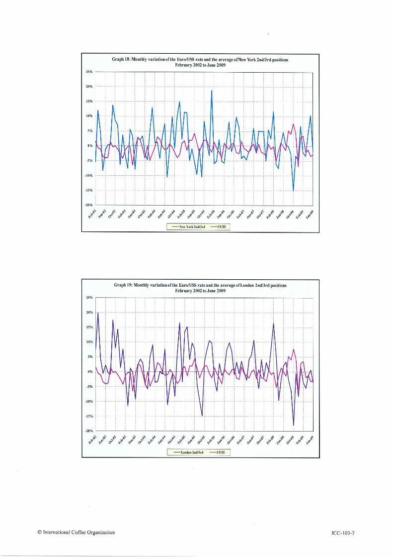
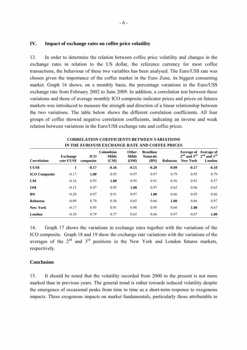
IV. Impact of exchange rates on coffee price volatility 13. In order to determine the relation between coffee price volatility and changes in the exchange rates in relation to the US dollar, the reference currency for most coffee transactions, the behaviour of these two variables has been analysed. The Euro/US$ rate was chosen given the importance of the coffee market in the Euro Zone, its biggest consuming market. Graph 16 shows, on a monthly basis, the percentage variations in the Euro/US$ exchange rate from February 2002 to June 2009. In addition, a correlation test between these variations and those of average monthly ICO composite indicator prices and prices on futures markets was introduced to measure the strength and direction of a linear relationship between the two variations. The table below shows the different correlation coefficients. All four groups of coffee showed negative correlation coefficients, indicating an inverse and weak relation between variations in the Euro/US$ exchange rate and coffee prices.

CORRELATION COEFFICIENTS BETWEEN VARIATIONS IN THE EURO/US$ EXCHANGE RATE AND COFFEE PRICES

Correlation Exchange

rate €/US$ICO

composite

Colombian Milds(CM)

OtherMilds (OM)

Brazilian Naturals

(BN) Robustas

Average of 2nd and 3rd

New York

Average of 2nd and 3rd

London

€/US$ 1 -0.17 -0.16 -0.15 -0.20 -0.09 -0.17 -0.10

ICO Composite -0.17 1.00 0.93 0.97 0.97 0.79 0.95 0.79

CM -0.16 0.93 1.00 0.95 0.91 0.56 0.91 0.57

OM -0.15 0.97 0.95 1.00 0.97 0.65 0.96 0.65

BN -0.20 0.97 0.91 0.97 1.00 0.66 0.95 0.66

Robustas -0.09 0.79 0.56 0.65 0.66 1.00 0.66 0.97

New York -0.17 0.95 0.91 0.96 0.95 0.66 1.00 0.67

London -0.10 0.79 0.57 0.65 0.66 0.97 0.67 1.00

14. Graph 17 shows the variations in exchange rates together with the variations of the ICO composite. Graph 18 and 19 show the exchange rate variations with the variations of the averages of the 2nd and 3rd positions in the New York and London futures markets, respectively. Conclusion 15. It should be noted that the volatility recorded from 2000 to the present is not more marked than in previous years. The general trend is rather towards reduced volatility despite the emergence of occasional peaks from time to time as a short-term response to exogenous impacts. These exogenous impacts on market fundamentals, particularly those attributable to

- 7 -

climatic problems, are phenomena that have always contributed to increased volatility following the creation of an imbalance between supply and demand. It would seem that in absence of any significant supply-side shocks, such as frosts, droughts and floods, price volatility is relatively attenuated. 16. As for the influence of fluctuations in exchange rates, partial analysis based on monthly variations indicates that a fall in the value of the dollar in relation to the Euro entails an increase in coffee prices. A more in-depth analysis would, however, make it possible to draw clearer conclusions.

INDEX OF GRAPHS Graph 1: ICO composite indicator price – monthly averages: January 1990 to July 2009 Graph 2: ICO group indicator prices – monthly averages: January 1990 to July 2009 Graph 3: Average of the 2nd and 3rd positions in New York and London futures markets:

Monthly averages: January 1990 to July 2009 Graph 4: Total production – Crop years 1989/90 to 2008/09 Graph 5: Total exports to all destinations – Calendar years 1990 to 2008 Graph 6: Gross opening stocks in exporting countries – Crop years 1989/90 to 2008/09 Graph 7: Imports of all forms of coffee from all sources – calendar years 1990 to 2008 Graph 8: World consumption – Calendar years 1990 to 2008 Graph 9: ICO composite indicator price and volatility index (+ trend line) – monthly:

January 1990 to July 2009 Graph 9a: ICO composite indicator price and volatility index (+ trend line) – monthly:

January 2000 to July 2009 Graph 9b: ICO composite indicator price and volatility index (+ trend line) – monthly:

January 2008 to July 2009 Graph 10: Colombian Milds indicator price and volatility index (+ trend line) – monthly:

January 1990 to July 2009 Graph 11: Other Milds indicator price and volatility index (+ trend line) – monthly:

January 1990 to July 2009 Graph 12: Brazilian Naturals indicator price and volatility index (+ trend line) – monthly:

January 1990 to July 2009 Graph 13: Robustas indicator price and volatility index (+ trend line) – monthly:

January 1990 to July 2009 Graph 14: Average of the 2nd and 3rd positions of the New York futures market and

volatility index (+ trend line) – monthly: January 1990 to July 2009 Graph 15: Average of the 2nd and 3rd positions of the London futures market and

volatility index (+ trend line) – monthly: January 1990 to July 2009 Graph 16: Monthly variations of the €/US$ rate: February 2002 to June 2009 Graph 17: Monthly variations of the €/US$ rate and the ICO composite indicator price:

February 2002 to June 2009 Graph 18: Monthly variations of the €/US$ rate and the average of the 2nd and

3rd positions in the New York futures market: February 2002 to June 2009 Graph 19: Monthly variations of the €/US$ rate and the average of the 2nd and

3rd positions in the London futures market: February 2002 to June 2009