IBM SAN Solution Design Best Practices for VMware vSphere ESXi

ibm.com/redbooks

Front cover

IBM SAN Solution Design Best Practices for VMware vSphere ESXi

Richard KelleyScheila Rossana Rinaldo Maliska

Leandro TorolhoMichael Voigt

Jon Tate

Learn about IBM b-type SAN fabricbest practices

Read about VMware best practices in a b-type SAN

Putting it all together inthe SAN

http://www.redbooks.ibm.com/


International Technical Support Organization


September 2013

SG24-8158-00

© Copyright International Business Machines Corporation 2013. All rights reserved.Note to U.S. Government Users Restricted Rights -- Use, duplication or disclosure restricted by GSA ADP ScheduleContract with IBM Corp.

First Edition (September 2013)

This edition applies to the hardware versions and software releases described in this publication only.

Note: Before using this information and the product it supports, read the information in “Notices” on page ix.

Contents

Notices . . . . . . . . . . . . . . . . . . . . . . . . . . . . . . . . . . . . . . . . . . . . . . . . . . . . . . . . . . . . . . . . . ixTrademarks . . . . . . . . . . . . . . . . . . . . . . . . . . . . . . . . . . . . . . . . . . . . . . . . . . . . . . . . . . . . . . .x

Preface . . . . . . . . . . . . . . . . . . . . . . . . . . . . . . . . . . . . . . . . . . . . . . . . . . . . . . . . . . . . . . . . . xiAuthors. . . . . . . . . . . . . . . . . . . . . . . . . . . . . . . . . . . . . . . . . . . . . . . . . . . . . . . . . . . . . . . . . . xiNow you can become a published author, too! . . . . . . . . . . . . . . . . . . . . . . . . . . . . . . . . . . xiiiComments welcome. . . . . . . . . . . . . . . . . . . . . . . . . . . . . . . . . . . . . . . . . . . . . . . . . . . . . . . xiiiStay connected to IBM Redbooks . . . . . . . . . . . . . . . . . . . . . . . . . . . . . . . . . . . . . . . . . . . . xiv

Chapter 1. Introduction. . . . . . . . . . . . . . . . . . . . . . . . . . . . . . . . . . . . . . . . . . . . . . . . . . . . 11.1 VMware vSphere ESXi . . . . . . . . . . . . . . . . . . . . . . . . . . . . . . . . . . . . . . . . . . . . . . . . . . 21.2 IBM Disk Storage Systems . . . . . . . . . . . . . . . . . . . . . . . . . . . . . . . . . . . . . . . . . . . . . . . 3

1.2.1 IBM Storwize V3700 . . . . . . . . . . . . . . . . . . . . . . . . . . . . . . . . . . . . . . . . . . . . . . . . 31.2.2 IBM Storwize V7000 . . . . . . . . . . . . . . . . . . . . . . . . . . . . . . . . . . . . . . . . . . . . . . . . 41.2.3 IBM SAN Volume Controller . . . . . . . . . . . . . . . . . . . . . . . . . . . . . . . . . . . . . . . . . . 5

1.3 IBM System Networking SAN b-type family . . . . . . . . . . . . . . . . . . . . . . . . . . . . . . . . . . 81.3.1 IBM System Storage SAN24B-5 (2498-F24) . . . . . . . . . . . . . . . . . . . . . . . . . . . . . 81.3.2 IBM System Storage SAN48B-5 (2498-F48) . . . . . . . . . . . . . . . . . . . . . . . . . . . . . 91.3.3 IBM System Storage SAN96B-5 (2498-F96 and 2498-N96). . . . . . . . . . . . . . . . . 101.3.4 IBM System Storage SAN384B-2 (2499-416) and SAN768B-2 (2499-816) . . . . . 11

Chapter 2. General SAN design and best practices. . . . . . . . . . . . . . . . . . . . . . . . . . . . 132.1 16 Gbps Fibre Channel . . . . . . . . . . . . . . . . . . . . . . . . . . . . . . . . . . . . . . . . . . . . . . . . . 14

2.1.1 Overview of 16 Gbps Fibre Channel . . . . . . . . . . . . . . . . . . . . . . . . . . . . . . . . . . . 142.2 Physical patching . . . . . . . . . . . . . . . . . . . . . . . . . . . . . . . . . . . . . . . . . . . . . . . . . . . . . 16

2.2.1 Using a structured approach. . . . . . . . . . . . . . . . . . . . . . . . . . . . . . . . . . . . . . . . . 172.2.2 Modular data cabling. . . . . . . . . . . . . . . . . . . . . . . . . . . . . . . . . . . . . . . . . . . . . . . 172.2.3 Cabling high-density, high port-count fiber equipment . . . . . . . . . . . . . . . . . . . . . 182.2.4 Using color to identify cables . . . . . . . . . . . . . . . . . . . . . . . . . . . . . . . . . . . . . . . . 192.2.5 Establishing a naming scheme . . . . . . . . . . . . . . . . . . . . . . . . . . . . . . . . . . . . . . . 192.2.6 Patch cables . . . . . . . . . . . . . . . . . . . . . . . . . . . . . . . . . . . . . . . . . . . . . . . . . . . . . 192.2.7 Patch panels . . . . . . . . . . . . . . . . . . . . . . . . . . . . . . . . . . . . . . . . . . . . . . . . . . . . . 202.2.8 Horizontal and backbone cables . . . . . . . . . . . . . . . . . . . . . . . . . . . . . . . . . . . . . . 202.2.9 Horizontal cable managers . . . . . . . . . . . . . . . . . . . . . . . . . . . . . . . . . . . . . . . . . . 202.2.10 Vertical cable managers . . . . . . . . . . . . . . . . . . . . . . . . . . . . . . . . . . . . . . . . . . . 202.2.11 Overhead cable pathways . . . . . . . . . . . . . . . . . . . . . . . . . . . . . . . . . . . . . . . . . 212.2.12 Cable ties . . . . . . . . . . . . . . . . . . . . . . . . . . . . . . . . . . . . . . . . . . . . . . . . . . . . . . 212.2.13 Implementing the cabling infrastructure . . . . . . . . . . . . . . . . . . . . . . . . . . . . . . . 212.2.14 Testing the links . . . . . . . . . . . . . . . . . . . . . . . . . . . . . . . . . . . . . . . . . . . . . . . . . 212.2.15 Building a common framework for the racks . . . . . . . . . . . . . . . . . . . . . . . . . . . . 212.2.16 Preserving the infrastructure. . . . . . . . . . . . . . . . . . . . . . . . . . . . . . . . . . . . . . . . 232.2.17 Documentation . . . . . . . . . . . . . . . . . . . . . . . . . . . . . . . . . . . . . . . . . . . . . . . . . . 232.2.18 Stocking spare cables. . . . . . . . . . . . . . . . . . . . . . . . . . . . . . . . . . . . . . . . . . . . . 232.2.19 Best practices for managing the cabling . . . . . . . . . . . . . . . . . . . . . . . . . . . . . . . 232.2.20 Summary. . . . . . . . . . . . . . . . . . . . . . . . . . . . . . . . . . . . . . . . . . . . . . . . . . . . . . . 25

2.3 Switch interconnections . . . . . . . . . . . . . . . . . . . . . . . . . . . . . . . . . . . . . . . . . . . . . . . . 252.3.1 Inter-switch link . . . . . . . . . . . . . . . . . . . . . . . . . . . . . . . . . . . . . . . . . . . . . . . . . . . 252.3.2 Inter-chassis links . . . . . . . . . . . . . . . . . . . . . . . . . . . . . . . . . . . . . . . . . . . . . . . . . 282.3.3 Fabric shortest path first . . . . . . . . . . . . . . . . . . . . . . . . . . . . . . . . . . . . . . . . . . . . 33

© Copyright IBM Corp. 2013. All rights reserved. iii

2.4 Device placement . . . . . . . . . . . . . . . . . . . . . . . . . . . . . . . . . . . . . . . . . . . . . . . . . . . . . 352.4.1 Traffic locality . . . . . . . . . . . . . . . . . . . . . . . . . . . . . . . . . . . . . . . . . . . . . . . . . . . . 352.4.2 Fan-in ratios and oversubscription . . . . . . . . . . . . . . . . . . . . . . . . . . . . . . . . . . . . 36

2.5 Data flow considerations . . . . . . . . . . . . . . . . . . . . . . . . . . . . . . . . . . . . . . . . . . . . . . . . 382.5.1 Congestion in the fabric . . . . . . . . . . . . . . . . . . . . . . . . . . . . . . . . . . . . . . . . . . . . 382.5.2 Traffic versus frame congestion . . . . . . . . . . . . . . . . . . . . . . . . . . . . . . . . . . . . . . 382.5.3 Sources of congestion . . . . . . . . . . . . . . . . . . . . . . . . . . . . . . . . . . . . . . . . . . . . . 382.5.4 Mitigating congestion with edge hold time . . . . . . . . . . . . . . . . . . . . . . . . . . . . . . 39

2.6 Host bus adapter . . . . . . . . . . . . . . . . . . . . . . . . . . . . . . . . . . . . . . . . . . . . . . . . . . . . . . 432.6.1 b-type host bus adapters . . . . . . . . . . . . . . . . . . . . . . . . . . . . . . . . . . . . . . . . . . . 432.6.2 QLogic. . . . . . . . . . . . . . . . . . . . . . . . . . . . . . . . . . . . . . . . . . . . . . . . . . . . . . . . . . 442.6.3 Emulex . . . . . . . . . . . . . . . . . . . . . . . . . . . . . . . . . . . . . . . . . . . . . . . . . . . . . . . . . 45

2.7 Zoning . . . . . . . . . . . . . . . . . . . . . . . . . . . . . . . . . . . . . . . . . . . . . . . . . . . . . . . . . . . . . . 452.8 Redundancy and resiliency . . . . . . . . . . . . . . . . . . . . . . . . . . . . . . . . . . . . . . . . . . . . . . 51

2.8.1 Single point of failure . . . . . . . . . . . . . . . . . . . . . . . . . . . . . . . . . . . . . . . . . . . . . . 522.9 Topologies. . . . . . . . . . . . . . . . . . . . . . . . . . . . . . . . . . . . . . . . . . . . . . . . . . . . . . . . . . . 53

2.9.1 Core-edge topology . . . . . . . . . . . . . . . . . . . . . . . . . . . . . . . . . . . . . . . . . . . . . . . 532.9.2 Edge-core-edge topology . . . . . . . . . . . . . . . . . . . . . . . . . . . . . . . . . . . . . . . . . . . 542.9.3 Full-mesh topology . . . . . . . . . . . . . . . . . . . . . . . . . . . . . . . . . . . . . . . . . . . . . . . . 55

2.10 Distance . . . . . . . . . . . . . . . . . . . . . . . . . . . . . . . . . . . . . . . . . . . . . . . . . . . . . . . . . . . 562.10.1 Buffer allocation . . . . . . . . . . . . . . . . . . . . . . . . . . . . . . . . . . . . . . . . . . . . . . . . . 562.10.2 Fabric interconnectivity over Fibre Channel at longer distances. . . . . . . . . . . . . 572.10.3 Fibre Channel over IP . . . . . . . . . . . . . . . . . . . . . . . . . . . . . . . . . . . . . . . . . . . . . 572.10.4 FCIP with FCR . . . . . . . . . . . . . . . . . . . . . . . . . . . . . . . . . . . . . . . . . . . . . . . . . . 592.10.5 Using EX_Ports and VEX_Ports . . . . . . . . . . . . . . . . . . . . . . . . . . . . . . . . . . . . . 602.10.6 Advanced FCIP configuration . . . . . . . . . . . . . . . . . . . . . . . . . . . . . . . . . . . . . . . 622.10.7 FCIP design best practices . . . . . . . . . . . . . . . . . . . . . . . . . . . . . . . . . . . . . . . . . 652.10.8 FCIP Trunking. . . . . . . . . . . . . . . . . . . . . . . . . . . . . . . . . . . . . . . . . . . . . . . . . . . 672.10.9 Virtual Fabrics . . . . . . . . . . . . . . . . . . . . . . . . . . . . . . . . . . . . . . . . . . . . . . . . . . . 692.10.10 Ethernet Interface Sharing . . . . . . . . . . . . . . . . . . . . . . . . . . . . . . . . . . . . . . . . 692.10.11 Workloads . . . . . . . . . . . . . . . . . . . . . . . . . . . . . . . . . . . . . . . . . . . . . . . . . . . . . 702.10.12 Intel based virtualization storage access . . . . . . . . . . . . . . . . . . . . . . . . . . . . . 71

2.11 Security . . . . . . . . . . . . . . . . . . . . . . . . . . . . . . . . . . . . . . . . . . . . . . . . . . . . . . . . . . . . 722.11.1 Zone management: Dynamic Fabric Provisioning . . . . . . . . . . . . . . . . . . . . . . . 722.11.2 Zone management: Duplicate WWNs. . . . . . . . . . . . . . . . . . . . . . . . . . . . . . . . . 722.11.3 Role-based access controls . . . . . . . . . . . . . . . . . . . . . . . . . . . . . . . . . . . . . . . . 732.11.4 Access control lists . . . . . . . . . . . . . . . . . . . . . . . . . . . . . . . . . . . . . . . . . . . . . . . 732.11.5 Policy database distribution . . . . . . . . . . . . . . . . . . . . . . . . . . . . . . . . . . . . . . . . 742.11.6 In-flight encryption and compression: b-type (16 Gbps) platforms only . . . . . . . 752.11.7 In-flight encryption and compression guidelines . . . . . . . . . . . . . . . . . . . . . . . . . 76

2.12 Monitoring . . . . . . . . . . . . . . . . . . . . . . . . . . . . . . . . . . . . . . . . . . . . . . . . . . . . . . . . . . 762.12.1 Fabric Watch. . . . . . . . . . . . . . . . . . . . . . . . . . . . . . . . . . . . . . . . . . . . . . . . . . . . 762.12.2 RAS log. . . . . . . . . . . . . . . . . . . . . . . . . . . . . . . . . . . . . . . . . . . . . . . . . . . . . . . . 772.12.3 Audit log . . . . . . . . . . . . . . . . . . . . . . . . . . . . . . . . . . . . . . . . . . . . . . . . . . . . . . . 772.12.4 SAN Health . . . . . . . . . . . . . . . . . . . . . . . . . . . . . . . . . . . . . . . . . . . . . . . . . . . . . 772.12.5 Design guidelines . . . . . . . . . . . . . . . . . . . . . . . . . . . . . . . . . . . . . . . . . . . . . . . . 772.12.6 Monitoring and notifications . . . . . . . . . . . . . . . . . . . . . . . . . . . . . . . . . . . . . . . . 77

2.13 Scalability, supportability, and performance . . . . . . . . . . . . . . . . . . . . . . . . . . . . . . . . 78

Chapter 3. General practices for VMware . . . . . . . . . . . . . . . . . . . . . . . . . . . . . . . . . . . . 813.1 VMware Pluggable Storage Architecture . . . . . . . . . . . . . . . . . . . . . . . . . . . . . . . . . . . 83

3.1.1 VMware NMP Flow of I/O . . . . . . . . . . . . . . . . . . . . . . . . . . . . . . . . . . . . . . . . . . . 843.1.2 Path Selection Plug-ins. . . . . . . . . . . . . . . . . . . . . . . . . . . . . . . . . . . . . . . . . . . . . 84

iv IBM SAN Solution Design Best Practices for VMware vSphere ESXi

3.2 Asymmetric Logical Unit Access . . . . . . . . . . . . . . . . . . . . . . . . . . . . . . . . . . . . . . . . . . 903.2.1 Path trashing. . . . . . . . . . . . . . . . . . . . . . . . . . . . . . . . . . . . . . . . . . . . . . . . . . . . . 923.2.2 Finding the optimized paths . . . . . . . . . . . . . . . . . . . . . . . . . . . . . . . . . . . . . . . . . 92

3.3 VMware vStorage APIs for Storage Awareness . . . . . . . . . . . . . . . . . . . . . . . . . . . . . . 943.3.1 Profile Driven Storage. . . . . . . . . . . . . . . . . . . . . . . . . . . . . . . . . . . . . . . . . . . . . . 97

3.4 Storage I/O Control . . . . . . . . . . . . . . . . . . . . . . . . . . . . . . . . . . . . . . . . . . . . . . . . . . . . 973.4.1 SIOC limitations and requirements . . . . . . . . . . . . . . . . . . . . . . . . . . . . . . . . . . . . 983.4.2 Storage I/O Control congestion latency . . . . . . . . . . . . . . . . . . . . . . . . . . . . . . . . 993.4.3 Conclusion . . . . . . . . . . . . . . . . . . . . . . . . . . . . . . . . . . . . . . . . . . . . . . . . . . . . . . 99

3.5 Storage Distributed Resource Scheduler . . . . . . . . . . . . . . . . . . . . . . . . . . . . . . . . . . . 993.5.1 Migration recommendations . . . . . . . . . . . . . . . . . . . . . . . . . . . . . . . . . . . . . . . . 1013.5.2 SDRS I/O balancing . . . . . . . . . . . . . . . . . . . . . . . . . . . . . . . . . . . . . . . . . . . . . . 1013.5.3 SDRS space balancing . . . . . . . . . . . . . . . . . . . . . . . . . . . . . . . . . . . . . . . . . . . . 1023.5.4 Schedule SDRS for off-peak hours . . . . . . . . . . . . . . . . . . . . . . . . . . . . . . . . . . . 1023.5.5 Conclusion . . . . . . . . . . . . . . . . . . . . . . . . . . . . . . . . . . . . . . . . . . . . . . . . . . . . . 103

3.6 Virtual Machine File System . . . . . . . . . . . . . . . . . . . . . . . . . . . . . . . . . . . . . . . . . . . . 1033.6.1 VMFS extents . . . . . . . . . . . . . . . . . . . . . . . . . . . . . . . . . . . . . . . . . . . . . . . . . . . 1053.6.2 Disk alignment . . . . . . . . . . . . . . . . . . . . . . . . . . . . . . . . . . . . . . . . . . . . . . . . . . 1053.6.3 Virtual machine files . . . . . . . . . . . . . . . . . . . . . . . . . . . . . . . . . . . . . . . . . . . . . . 107

3.7 VMware vMotion . . . . . . . . . . . . . . . . . . . . . . . . . . . . . . . . . . . . . . . . . . . . . . . . . . . . . 1073.8 VMware storage vMotion . . . . . . . . . . . . . . . . . . . . . . . . . . . . . . . . . . . . . . . . . . . . . . 1093.9 vStorage APIs for Array Integration . . . . . . . . . . . . . . . . . . . . . . . . . . . . . . . . . . . . . . 111

3.9.1 Requirements . . . . . . . . . . . . . . . . . . . . . . . . . . . . . . . . . . . . . . . . . . . . . . . . . . . 1143.9.2 Confirming VAAI Hardware Acceleration is detected . . . . . . . . . . . . . . . . . . . . . 1143.9.3 Setting the data transfer chunk size . . . . . . . . . . . . . . . . . . . . . . . . . . . . . . . . . . 117

3.10 Raw Device Mapping . . . . . . . . . . . . . . . . . . . . . . . . . . . . . . . . . . . . . . . . . . . . . . . . 1183.11 VMware thin provisioning . . . . . . . . . . . . . . . . . . . . . . . . . . . . . . . . . . . . . . . . . . . . . 120

3.11.1 Using VMFS thin provisioning. . . . . . . . . . . . . . . . . . . . . . . . . . . . . . . . . . . . . . 1213.11.2 Thin provisioning prerequisites . . . . . . . . . . . . . . . . . . . . . . . . . . . . . . . . . . . . . 1223.11.3 Thin provisioning general guidelines. . . . . . . . . . . . . . . . . . . . . . . . . . . . . . . . . 1223.11.4 Thin on thin? . . . . . . . . . . . . . . . . . . . . . . . . . . . . . . . . . . . . . . . . . . . . . . . . . . . 123

3.12 IBM Storage Management Console for VMware vCenter . . . . . . . . . . . . . . . . . . . . . 1243.12.1 Conclusion . . . . . . . . . . . . . . . . . . . . . . . . . . . . . . . . . . . . . . . . . . . . . . . . . . . . 128

3.13 General recommendation . . . . . . . . . . . . . . . . . . . . . . . . . . . . . . . . . . . . . . . . . . . . . 128

Chapter 4. General practices for storage . . . . . . . . . . . . . . . . . . . . . . . . . . . . . . . . . . . 1334.1 Configuring and servicing external storage systems. . . . . . . . . . . . . . . . . . . . . . . . . . 134

4.1.1 General guidelines for SAN Volume Controller. . . . . . . . . . . . . . . . . . . . . . . . . . 1344.1.2 General Guidelines for Storwize V7000 . . . . . . . . . . . . . . . . . . . . . . . . . . . . . . . 1344.1.3 Configuring the Storwize V3700 . . . . . . . . . . . . . . . . . . . . . . . . . . . . . . . . . . . . . 1354.1.4 Storwize family presets . . . . . . . . . . . . . . . . . . . . . . . . . . . . . . . . . . . . . . . . . . . . 136

4.2 Disk . . . . . . . . . . . . . . . . . . . . . . . . . . . . . . . . . . . . . . . . . . . . . . . . . . . . . . . . . . . . . . . 1394.2.1 Input/output operations per second . . . . . . . . . . . . . . . . . . . . . . . . . . . . . . . . . . 1394.2.2 Disk types . . . . . . . . . . . . . . . . . . . . . . . . . . . . . . . . . . . . . . . . . . . . . . . . . . . . . . 140

4.3 MDisks and volumes . . . . . . . . . . . . . . . . . . . . . . . . . . . . . . . . . . . . . . . . . . . . . . . . . . 1414.3.1 Disk tiering . . . . . . . . . . . . . . . . . . . . . . . . . . . . . . . . . . . . . . . . . . . . . . . . . . . . . 1414.3.2 Logical disk configuration guidelines for storage systems . . . . . . . . . . . . . . . . . 1434.3.3 RAID configuration guidelines for storage systems . . . . . . . . . . . . . . . . . . . . . . 1434.3.4 Optimal storage pool configuration guidelines for storage systems . . . . . . . . . . 1444.3.5 FlashCopy mapping guidelines for storage systems. . . . . . . . . . . . . . . . . . . . . . 1454.3.6 Image mode volumes and data migration guidelines for storage systems . . . . . 1464.3.7 Configuring a balanced storage system . . . . . . . . . . . . . . . . . . . . . . . . . . . . . . . 147

4.4 Volumes . . . . . . . . . . . . . . . . . . . . . . . . . . . . . . . . . . . . . . . . . . . . . . . . . . . . . . . . . . . 150

Contents v

4.4.1 Thin provisioning. . . . . . . . . . . . . . . . . . . . . . . . . . . . . . . . . . . . . . . . . . . . . . . . . 1504.5 Back-end . . . . . . . . . . . . . . . . . . . . . . . . . . . . . . . . . . . . . . . . . . . . . . . . . . . . . . . . . . . 1534.6 Front-end/fabric . . . . . . . . . . . . . . . . . . . . . . . . . . . . . . . . . . . . . . . . . . . . . . . . . . . . . . 153

4.6.1 4-way multipathing . . . . . . . . . . . . . . . . . . . . . . . . . . . . . . . . . . . . . . . . . . . . . . . 1554.6.2 8-way multipathing . . . . . . . . . . . . . . . . . . . . . . . . . . . . . . . . . . . . . . . . . . . . . . . 1574.6.3 Greater than 8-way multipathing . . . . . . . . . . . . . . . . . . . . . . . . . . . . . . . . . . . . . 159

4.7 VMware considerations. . . . . . . . . . . . . . . . . . . . . . . . . . . . . . . . . . . . . . . . . . . . . . . . 1614.7.1 Configuring the QLogic HBA for hosts running the VMware OS. . . . . . . . . . . . . 1614.7.2 Queue depth . . . . . . . . . . . . . . . . . . . . . . . . . . . . . . . . . . . . . . . . . . . . . . . . . . . . 162

4.8 Maintenance considerations . . . . . . . . . . . . . . . . . . . . . . . . . . . . . . . . . . . . . . . . . . . . 1634.9 Putting it all together . . . . . . . . . . . . . . . . . . . . . . . . . . . . . . . . . . . . . . . . . . . . . . . . . . 1634.10 References . . . . . . . . . . . . . . . . . . . . . . . . . . . . . . . . . . . . . . . . . . . . . . . . . . . . . . . . 164

Chapter 5. Business continuity and disaster recovery . . . . . . . . . . . . . . . . . . . . . . . . . . . . . . . . . . . . . . . . . . . . . 165

5.1 Continuity and recovery solutions . . . . . . . . . . . . . . . . . . . . . . . . . . . . . . . . . . . . . . . . 1665.2 IBM Replication Family Services. . . . . . . . . . . . . . . . . . . . . . . . . . . . . . . . . . . . . . . . . 166

5.2.1 FlashCopy. . . . . . . . . . . . . . . . . . . . . . . . . . . . . . . . . . . . . . . . . . . . . . . . . . . . . . 1665.2.2 Metro Mirror . . . . . . . . . . . . . . . . . . . . . . . . . . . . . . . . . . . . . . . . . . . . . . . . . . . . 1685.2.3 Global Mirror . . . . . . . . . . . . . . . . . . . . . . . . . . . . . . . . . . . . . . . . . . . . . . . . . . . . 1705.2.4 Image mode migration and volume mirroring migration . . . . . . . . . . . . . . . . . . . 172

5.3 IBM SAN Volume Controller Stretched Cluster . . . . . . . . . . . . . . . . . . . . . . . . . . . . . . 1735.4 VMware vSphere Fault Tolerance. . . . . . . . . . . . . . . . . . . . . . . . . . . . . . . . . . . . . . . . 1775.5 VMware vSphere vMotion and VMware vSphere HA . . . . . . . . . . . . . . . . . . . . . . . . . 179

5.5.1 VMware vSphere vMotion . . . . . . . . . . . . . . . . . . . . . . . . . . . . . . . . . . . . . . . . . . 1795.5.2 VMware vSphere High Availability . . . . . . . . . . . . . . . . . . . . . . . . . . . . . . . . . . . 1795.5.3 VMware vSphere Metro Storage Cluster . . . . . . . . . . . . . . . . . . . . . . . . . . . . . . 1825.5.4 VMware vCenter Site Recovery Manager. . . . . . . . . . . . . . . . . . . . . . . . . . . . . . 185

5.6 Storage Replication Adapter for IBM SAN Volume Controller. . . . . . . . . . . . . . . . . . . 1905.7 Backup and restore solutions . . . . . . . . . . . . . . . . . . . . . . . . . . . . . . . . . . . . . . . . . . . 1915.8 Traditional backup and restore with Tivoli Storage Manager . . . . . . . . . . . . . . . . . . . 192

5.8.1 Disaster recovery manager. . . . . . . . . . . . . . . . . . . . . . . . . . . . . . . . . . . . . . . . . 1935.9 Tivoli Storage Manager for Virtual Environments . . . . . . . . . . . . . . . . . . . . . . . . . . . . 1945.10 VMware vSphere Data Protection. . . . . . . . . . . . . . . . . . . . . . . . . . . . . . . . . . . . . . . 197

Chapter 6. Entry level scenario . . . . . . . . . . . . . . . . . . . . . . . . . . . . . . . . . . . . . . . . . . . 2016.1 Storage area network . . . . . . . . . . . . . . . . . . . . . . . . . . . . . . . . . . . . . . . . . . . . . . . . . 202

6.1.1 Topology . . . . . . . . . . . . . . . . . . . . . . . . . . . . . . . . . . . . . . . . . . . . . . . . . . . . . . . 2026.1.2 Naming convention and zoning scheme . . . . . . . . . . . . . . . . . . . . . . . . . . . . . . . 2036.1.3 16 Gb Fibre Channel host bus adapters . . . . . . . . . . . . . . . . . . . . . . . . . . . . . . . 204

6.2 Storage subsystem . . . . . . . . . . . . . . . . . . . . . . . . . . . . . . . . . . . . . . . . . . . . . . . . . . . 2056.2.1 Preparing for Fibre Channel attachment . . . . . . . . . . . . . . . . . . . . . . . . . . . . . . . 2056.2.2 VMware ESXi installation . . . . . . . . . . . . . . . . . . . . . . . . . . . . . . . . . . . . . . . . . . 2066.2.3 VMware ESXi multipathing . . . . . . . . . . . . . . . . . . . . . . . . . . . . . . . . . . . . . . . . . 2066.2.4 VMware license considerations. . . . . . . . . . . . . . . . . . . . . . . . . . . . . . . . . . . . . . 2076.2.5 VMware support contracts . . . . . . . . . . . . . . . . . . . . . . . . . . . . . . . . . . . . . . . . . 2086.2.6 Backup and disaster recovery. . . . . . . . . . . . . . . . . . . . . . . . . . . . . . . . . . . . . . . 209

Chapter 7. Midrange level scenario . . . . . . . . . . . . . . . . . . . . . . . . . . . . . . . . . . . . . . . . 2117.1 Storage area network . . . . . . . . . . . . . . . . . . . . . . . . . . . . . . . . . . . . . . . . . . . . . . . . . 212

7.1.1 Topology . . . . . . . . . . . . . . . . . . . . . . . . . . . . . . . . . . . . . . . . . . . . . . . . . . . . . . . 2127.1.2 Naming convention and zoning scheme . . . . . . . . . . . . . . . . . . . . . . . . . . . . . . . 213

7.2 Storage subsystem . . . . . . . . . . . . . . . . . . . . . . . . . . . . . . . . . . . . . . . . . . . . . . . . . . . 2157.2.1 Preparing for Fibre Channel attachment . . . . . . . . . . . . . . . . . . . . . . . . . . . . . . . 216

vi IBM SAN Solution Design Best Practices for VMware vSphere ESXi

7.2.2 VMware ESXi installation . . . . . . . . . . . . . . . . . . . . . . . . . . . . . . . . . . . . . . . . . . 2177.2.3 VMware ESXi multipathing . . . . . . . . . . . . . . . . . . . . . . . . . . . . . . . . . . . . . . . . . 218

7.3 VMware considerations. . . . . . . . . . . . . . . . . . . . . . . . . . . . . . . . . . . . . . . . . . . . . . . . 2197.3.1 Backup and disaster recovery. . . . . . . . . . . . . . . . . . . . . . . . . . . . . . . . . . . . . . . 219

Chapter 8. Enterprise scenario . . . . . . . . . . . . . . . . . . . . . . . . . . . . . . . . . . . . . . . . . . . 2218.1 Introduction . . . . . . . . . . . . . . . . . . . . . . . . . . . . . . . . . . . . . . . . . . . . . . . . . . . . . . . . . 2228.2 Fabric types. . . . . . . . . . . . . . . . . . . . . . . . . . . . . . . . . . . . . . . . . . . . . . . . . . . . . . . . . 224

8.2.1 Edge-core-edge topology . . . . . . . . . . . . . . . . . . . . . . . . . . . . . . . . . . . . . . . . . . 2258.2.2 Device placement . . . . . . . . . . . . . . . . . . . . . . . . . . . . . . . . . . . . . . . . . . . . . . . . 226

8.3 Edge-core-edge design. . . . . . . . . . . . . . . . . . . . . . . . . . . . . . . . . . . . . . . . . . . . . . . . 2288.3.1 Storage edge . . . . . . . . . . . . . . . . . . . . . . . . . . . . . . . . . . . . . . . . . . . . . . . . . . . 2298.3.2 Trunk groups. . . . . . . . . . . . . . . . . . . . . . . . . . . . . . . . . . . . . . . . . . . . . . . . . . . . 2298.3.3 Storwize V7000. . . . . . . . . . . . . . . . . . . . . . . . . . . . . . . . . . . . . . . . . . . . . . . . . . 2328.3.4 SAN Volume Controller and core . . . . . . . . . . . . . . . . . . . . . . . . . . . . . . . . . . . . 2338.3.5 Host edge . . . . . . . . . . . . . . . . . . . . . . . . . . . . . . . . . . . . . . . . . . . . . . . . . . . . . . 235

8.4 Zoning . . . . . . . . . . . . . . . . . . . . . . . . . . . . . . . . . . . . . . . . . . . . . . . . . . . . . . . . . . . . . 2378.4.1 Types of zoning. . . . . . . . . . . . . . . . . . . . . . . . . . . . . . . . . . . . . . . . . . . . . . . . . . 2378.4.2 Prezoning tips and shortcuts. . . . . . . . . . . . . . . . . . . . . . . . . . . . . . . . . . . . . . . . 2398.4.3 SAN Volume Controller internode communications zone . . . . . . . . . . . . . . . . . . 2398.4.4 SAN Volume Controller storage zones . . . . . . . . . . . . . . . . . . . . . . . . . . . . . . . . 2398.4.5 Storwize V7000 storage subsystem . . . . . . . . . . . . . . . . . . . . . . . . . . . . . . . . . . 2408.4.6 SAN Volume Controller host zones. . . . . . . . . . . . . . . . . . . . . . . . . . . . . . . . . . . 2408.4.7 Standard SAN Volume Controller zoning configuration . . . . . . . . . . . . . . . . . . . 2428.4.8 Aliases . . . . . . . . . . . . . . . . . . . . . . . . . . . . . . . . . . . . . . . . . . . . . . . . . . . . . . . . 2428.4.9 Zones . . . . . . . . . . . . . . . . . . . . . . . . . . . . . . . . . . . . . . . . . . . . . . . . . . . . . . . . . 2448.4.10 Zoning with multiple SAN Volume Controller clustered systems . . . . . . . . . . . 2468.4.11 Split storage subsystem configurations. . . . . . . . . . . . . . . . . . . . . . . . . . . . . . . 246

8.5 Switch domain IDs . . . . . . . . . . . . . . . . . . . . . . . . . . . . . . . . . . . . . . . . . . . . . . . . . . . 2468.6 Tying it all together . . . . . . . . . . . . . . . . . . . . . . . . . . . . . . . . . . . . . . . . . . . . . . . . . . . 246

8.6.1 Setting up aliases . . . . . . . . . . . . . . . . . . . . . . . . . . . . . . . . . . . . . . . . . . . . . . . . 2468.7 VMware enterprise level . . . . . . . . . . . . . . . . . . . . . . . . . . . . . . . . . . . . . . . . . . . . . . . 254

8.7.1 Backup and disaster recovery. . . . . . . . . . . . . . . . . . . . . . . . . . . . . . . . . . . . . . . 2568.8 References . . . . . . . . . . . . . . . . . . . . . . . . . . . . . . . . . . . . . . . . . . . . . . . . . . . . . . . . . 258

Related publications . . . . . . . . . . . . . . . . . . . . . . . . . . . . . . . . . . . . . . . . . . . . . . . . . . . . 259IBM Redbooks . . . . . . . . . . . . . . . . . . . . . . . . . . . . . . . . . . . . . . . . . . . . . . . . . . . . . . . . . . 259Help from IBM . . . . . . . . . . . . . . . . . . . . . . . . . . . . . . . . . . . . . . . . . . . . . . . . . . . . . . . . . . 259

Contents vii

viii IBM SAN Solution Design Best Practices for VMware vSphere ESXi

Notices

This information was developed for products and services offered in the U.S.A.

IBM may not offer the products, services, or features discussed in this document in other countries. Consult your local IBM representative for information on the products and services currently available in your area. Any reference to an IBM product, program, or service is not intended to state or imply that only that IBM product, program, or service may be used. Any functionally equivalent product, program, or service that does not infringe any IBM intellectual property right may be used instead. However, it is the user's responsibility to evaluate and verify the operation of any non-IBM product, program, or service.

IBM may have patents or pending patent applications covering subject matter described in this document. The furnishing of this document does not grant you any license to these patents. You can send license inquiries, in writing, to: IBM Director of Licensing, IBM Corporation, North Castle Drive, Armonk, NY 10504-1785 U.S.A.

The following paragraph does not apply to the United Kingdom or any other country where such provisions are inconsistent with local law: INTERNATIONAL BUSINESS MACHINES CORPORATION PROVIDES THIS PUBLICATION "AS IS" WITHOUT WARRANTY OF ANY KIND, EITHER EXPRESS OR IMPLIED, INCLUDING, BUT NOT LIMITED TO, THE IMPLIED WARRANTIES OF NON-INFRINGEMENT, MERCHANTABILITY OR FITNESS FOR A PARTICULAR PURPOSE. Some states do not allow disclaimer of express or implied warranties in certain transactions, therefore, this statement may not apply to you.

This information could include technical inaccuracies or typographical errors. Changes are periodically made to the information herein; these changes will be incorporated in new editions of the publication. IBM may make improvements and/or changes in the product(s) and/or the program(s) described in this publication at any time without notice.

Any references in this information to non-IBM websites are provided for convenience only and do not in any manner serve as an endorsement of those websites. The materials at those websites are not part of the materials for this IBM product and use of those websites is at your own risk.

IBM may use or distribute any of the information you supply in any way it believes appropriate without incurring any obligation to you.

Any performance data contained herein was determined in a controlled environment. Therefore, the results obtained in other operating environments may vary significantly. Some measurements may have been made on development-level systems and there is no guarantee that these measurements will be the same on generally available systems. Furthermore, some measurements may have been estimated through extrapolation. Actual results may vary. Users of this document should verify the applicable data for their specific environment.

Information concerning non-IBM products was obtained from the suppliers of those products, their published announcements or other publicly available sources. IBM has not tested those products and cannot confirm the accuracy of performance, compatibility or any other claims related to non-IBM products. Questions on the capabilities of non-IBM products should be addressed to the suppliers of those products.

This information contains examples of data and reports used in daily business operations. To illustrate them as completely as possible, the examples include the names of individuals, companies, brands, and products. All of these names are fictitious and any similarity to the names and addresses used by an actual business enterprise is entirely coincidental.

COPYRIGHT LICENSE:

This information contains sample application programs in source language, which illustrate programming techniques on various operating platforms. You may copy, modify, and distribute these sample programs in any form without payment to IBM, for the purposes of developing, using, marketing or distributing application programs conforming to the application programming interface for the operating platform for which the sample programs are written. These examples have not been thoroughly tested under all conditions. IBM, therefore, cannot guarantee or imply reliability, serviceability, or function of these programs.

© Copyright IBM Corp. 2013. All rights reserved. ix

Trademarks

IBM, the IBM logo, and ibm.com are trademarks or registered trademarks of International Business Machines Corporation in the United States, other countries, or both. These and other IBM trademarked terms are marked on their first occurrence in this information with the appropriate symbol (® or ™), indicating US registered or common law trademarks owned by IBM at the time this information was published. Such trademarks may also be registered or common law trademarks in other countries. A current list of IBM trademarks is available on the Web at http://www.ibm.com/legal/copytrade.shtml

The following terms are trademarks of the International Business Machines Corporation in the United States, other countries, or both:

DS4000®DS8000®Easy Tier®FICON®FlashCopy®

IBM®Real-time Compression™Redbooks®Redbooks (logo) ®Storwize®

System Storage®System x®Tivoli Storage Manager FastBack®Tivoli®XIV®

The following terms are trademarks of other companies:

Intel, Intel logo, Intel Inside logo, and Intel Centrino logo are trademarks or registered trademarks of Intel Corporation or its subsidiaries in the United States and other countries.

Linux is a trademark of Linus Torvalds in the United States, other countries, or both.

Microsoft, Windows, and the Windows logo are trademarks of Microsoft Corporation in the United States, other countries, or both.

UNIX is a registered trademark of The Open Group in the United States and other countries.

Other company, product, or service names may be trademarks or service marks of others.

x IBM SAN Solution Design Best Practices for VMware vSphere ESXi

http://www.ibm.com/legal/copytrade.shtml

Preface

In this IBM® Redbooks® publication, we describe recommendations based on an IBM b-type storage area network (SAN) environment that is utilizing VMware vSphere ESXi. We describe the hardware and software and the unique features that they bring to the marketplace. We then highlight those features and how they apply to the SAN environment, and the best practices for ensuring that you get the best out of your SAN.

For background reading, we recommend the following Redbooks publications:

� Introduction to Storage Area Networks and System Networking, SG24-5470

� IBM System Storage SAN Volume Controller Best Practices and Performance Guidelines, SG24-7521

� IBM System Storage SAN Volume Controller and Storwize V7000 Replication Family Services, SG24-7574

� Implementing the IBM System Storage SAN Volume Controller V6.3, SG24-7933

� IBM SAN Volume Controller Stretched Cluster with PowerVM and PowerHA, SG24-8142

� Implementing the IBM SAN Volume Controller and FlashSystem 820, SG24-8172

� IBM System Storage DS8000 Copy Services for Open Systems, SG24-6788

� IBM System Storage DS8000: Host Attachment and Interoperability, SG24-8887

This book is aimed at pre- and post-sales support, system administrators, and storage administrators.

Authors

This book was produced by a team of specialists from around the world working at the IBM International Technical Support Organization (ITSO), San Jose Center.

Richard Kelley is a Team Lead and Subject Matter Expert (SME) with the Columbia storage area network (SAN)/disk delivery team for IBM US. He has 15 years experience in information technology (IT) supporting servers, operating systems, and networks in complex environments, and 5+ years experience in the SAN environment.

© Copyright IBM Corp. 2013. All rights reserved. xi

Scheila Rossana Rinaldo Maliska is an IT Specialist and has been working in England for the past 10 years. She has 21+ years experience in the IT Industry. Throughout her career, she has played a part in numerous project implementations including Enterprise Network Administration/Research and Development/Disaster Recovery/Replication/Virtualization, Consultancy, and Project Management on a large scale. For the last five years, she has been working in IBM Business Continuity and Resilience Services participating in complex disaster recovery tests, invocations, and implementations. Recently, she moved to be a VMware Specialist under IBM ITS Data Center Services, accountable for providing high-quality consultancy, design, and implementation services for clients within the UKISA region. She has a degree in Computer Science and an MBA (lato sensu) in Strategic Management of Information Technology, and holds three VMware certifications, including VMware Certified Professional 5 - Data Center Virtualization (VCP5-DCV).

Leandro Torolho is a SAN Storage Specialist for IBM Global Services in Brazil. Since joining IBM in 2007, Leandro has been the SAN storage subject matter expert (SME) for many international clients and he is also an IBM Certified IT Specialist (Level 2). He holds a Bachelor’s degree in Computer Science from Universidade Municipal de São Caetano do Sul in São Paulo, Brazil. He also has a post graduation degree in Computer Networks from Faculdades Associadas de São Paulo in Brazil.

Michael Voigt joined IBM in 2001. He is a co-founder of the “VMware Competence Center” within IBM Germany, responsible for providing implementation guidance and architectural governance to virtualize IBM data centers. Michael was a key player in creating the Global Virtualization Architecture, which included internal IBM security certification to allow multi-tenant client offerings, which has been the basis for the IBM Virtual Server and Cloud offerings. Currently, Michael is helping to drive the IBM Cloud Virtualization Strategy as a VMware Architect on the Smart Cloud Enterprise Plus (SCE+) to deliver fully serviced virtual machines to the IBM outsourcing clients. Michael has obtained VMware Certified Design Expert (VCDX) certification.

Jon Tate is a Project Manager for IBM System Storage® SAN Solutions at the ITSO, San Jose Center. Before joining the ITSO in 1999, he worked in the IBM Technical Support Center, providing Level 2/3 support for IBM storage products. Jon has 27 years of experience in storage software and management, services, and support, and is both an IBM Certified IT Specialist and an IBM SAN Certified Specialist. He is also the UK Chairman of the Storage Networking Industry Association.

xii IBM SAN Solution Design Best Practices for VMware vSphere ESXi

Thanks to the following people for their contributions to this project:

Sangam RacherlaInternational Technical Support Organization, San Jose Center

Paul KohlerLucas NguyenRawlinson RiveraVMware

Special thanks to the Brocade Communications Systems staff in San Jose, California for their unparalleled support of this residency in terms of equipment and support in many areas:

Michael AtkinsonJim BaldygaHor-May ChanSilviano GaonaBrian LarsenBlayne RawskyBrian StefflerMarcus ThordalSteven TongBrocade Communications Systems

Now you can become a published author, too!

Here’s an opportunity to spotlight your skills, grow your career, and become a published author—all at the same time! Join an ITSO residency project and help write a book in your area of expertise, while honing your experience using leading-edge technologies. Your efforts will help to increase product acceptance and customer satisfaction, as you expand your network of technical contacts and relationships. Residencies run from two to six weeks in length, and you can participate either in person or as a remote resident working from your home base.

Find out more about the residency program, browse the residency index, and apply online at:

ibm.com/redbooks/residencies.html

Comments welcome

Your comments are important to us!

We want our books to be as helpful as possible. Send us your comments about this book or other IBM Redbooks publications in one of the following ways:

� Use the online Contact us review Redbooks form found at:

ibm.com/redbooks

� Send your comments in an email to:

[email protected]

Preface xiii

http://www.redbooks.ibm.com/residencies.html

http://www.redbooks.ibm.com/residencies.html



http://www.redbooks.ibm.com/contacts.html

� Mail your comments to:

IBM Corporation, International Technical Support OrganizationDept. HYTD Mail Station P0992455 South RoadPoughkeepsie, NY 12601-5400

Stay connected to IBM Redbooks

� Find us on Facebook:

http://www.facebook.com/IBMRedbooks

� Follow us on Twitter:

http://twitter.com/ibmredbooks

� Look for us on LinkedIn:

http://www.linkedin.com/groups?home=&gid=2130806

� Explore new Redbooks publications, residencies, and workshops with the IBM Redbooks weekly newsletter:

https://www.redbooks.ibm.com/Redbooks.nsf/subscribe?OpenForm

� Stay current on recent Redbooks publications with RSS Feeds:

http://www.redbooks.ibm.com/rss.html

xiv IBM SAN Solution Design Best Practices for VMware vSphere ESXi

http://www.facebook.com/IBMRedbooks

http://twitter.com/ibmredbooks

http://www.linkedin.com/groups?home=&gid=2130806

https://www.redbooks.ibm.com/Redbooks.nsf/subscribe?OpenForm

http://www.redbooks.ibm.com/rss.html

Chapter 1. Introduction

Virtualization has become a common practice in today’s world, and with that comes the challenges for configuring the storage and the fabric behind the virtual environments. Business Continuity is also indispensable these days if you want to protect your business from major failures, and with the latest advances in technology, long-distance solutions are now adding even more resilience to your environment.

The intent of this book is to provide an overview of the best practices for specific IBM storage area network (SAN) systems and switches, which are listed in this chapter, and their utilization with VMware vSphere ESXi. We also describe the most common business continuity technologies, and the different scenarios for entry, midrange, and enterprise environments.

This chapter includes the following sections:

� VMware vSphere ESXi

� IBM Disk Storage Systems

– IBM Storwize® V3700– IBM Storwize V7000– IBM SAN Volume Controller (SVC)

� IBM System Networking SAN b-type family

– IBM System Storage SAN24B-5 (2498-F24)– IBM System Storage SAN48B-5 (2498-F48)– IBM System Storage SAN96B-5 (2498-F96 and 2498-N96)– IBM System Storage SAN384B-2 (2499-416) and SAN768b-2 (2499-816)

1

© Copyright IBM Corp. 2013. All rights reserved. 1

1.1 VMware vSphere ESXi

VMware, Inc. was founded in 1998 to bring virtual machine (VM) technology to industry-standard computers. More information about VMware can be found at the following website:

http://www.vmware.com

The version of VMware vSphere ESXi covered in this book is 5.1, and we advise checking with VMware for any future release changes.

VMware vSphere ESXi 5.1 (at the time of writing) is the latest version of a virtualization software that enables the deployment of multiple, secure, independent virtual machines on a single physical server.

Figure 1-1 shows a comparison between the traditional Intel architecture and the VMware vSphere ESXi Server installed on Intel architecture. This diagram shows that VMware presents individual virtual hardware to each virtual machine. In this way, the operating systems and applications installed in the virtual machines are not aware that the hardware is virtual.

Figure 1-1 Comparison between a traditional Intel architecture and VMware vSphere ESXi Server

Due to the virtualization, the guest operating system is not aware where the resources, for example, CPU and memory are coming from.

One virtual machine is isolated from the other, and this is possible because of the virtualization layer and it enables the sharing of physical devices with the virtual machines. The resources do not materialize from thin air though, and an associated physical device or pool of resources needs to be available for providing resources to the virtual machines.

Later in this book, we describe virtualization techniques that are available today and that can help you respond to your business needs, enabling resilience and fast recoveries from a failure.

2 IBM SAN Solution Design Best Practices for VMware vSphere ESXi

http://www.vmware.com

1.2 IBM Disk Storage Systems

A storage area network (SAN) is made of shared storage devices; whereas, a storage device can be a disk drive, tape drive, optical drive, and these are available to the servers connected to them, showing as a local-attached device to the operating system. In this part of the book, we cover some of the disk storage systems that IBM provides and they are mentioned throughout the book.

For the latest information about the products that we describe, see the following website:

http://www.ibm.com/systems/storage/storwize/index.html

1.2.1 IBM Storwize V3700

The IBM Storwize V3700 is a simple and easy to use solution that can be used for entry and midrange businesses. The internal storage is configured with traditional Redundant Array of Independent Disks (RAID) systems and virtual disks are created from these.

Storwize V3700 provides the following benefits:

� Easy to use embedded graphical interface

� Supports solid-state drives (SSDs)

� Provides internal virtualization and thin provisioning for rapid deployment

� Capabilities and functions that are only normally provided in enterprise systems

� Incremental growth of storage capacity

� Ideal for VMware environments

– Improves performance and consolidation capabilities with vStorage APIs for Array Integration (VAAI) support that off loads I/O-intense storage

– With built-in IBM FlashCopy® technology for data protection, application testing, and virtual machine cloning

� The capacity can be up to 180 TB

Following, we describe the current Storwize V3700 models that are available at the time of writing of this book.

Figure 1-2 shows the front view of the 2072-12C and 12E enclosures.

Figure 1-2 IBM Storwize V3700 front view for 2072-12C and 12E enclosures

Chapter 1. Introduction 3

http://www.ibm.com/systems/storage/storwize/index.html

Figure 1-3 shows the front view of the 2072-24C and 24E enclosures.

Figure 1-3 IBM Storwize V3700 front view for 2072-24C and 24E enclosures

For the latest information about IBM Storwize V3700, see this website:

http://www.ibm.com/systems/storage/disk/storwize_v3700/index.html

Refer to the following IBM Redbooks publication for more information:

Implementing the IBM Storwize V3700, SG24-8107

1.2.2 IBM Storwize V7000

The IBM Storwize V7000 has a highly scalable capacity, superior performance, and high availability through its workload consolidation into a single storage system, which can also help to reduce costs and is ideal for midrange businesses.

IBM Storwize V7000 provides the following benefits:

� Built-in solid-state drive optimization

� Thin provisioning and nondisruptive migration of data

� Real-time compression for efficiently reducing disk capacity by up to 80%

� IBM System Storage Easy Tier® for automatically migrating data between storage tiers

� Easy to use graphical user interface

� Supports block workloads for simplicity and greater efficiency

� Resilience with IBM FlashCopy technology

� Metro Mirror and Global Mirror for replicating data synchronously or asynchronously between systems for backup efficiency

� Configurations up to 360 TB physical storage

Following, we show the current models that are available at the time of this writing.

Figure 1-4 shows the front view of the 2076-112 and 2076-312 enclosures.

Figure 1-4 IBM Storwize V7000 2076-112 and 2076-312 controllers



Figure 1-5 shows the front view of the 2076-124 and 2076-324 enclosures.

Figure 1-5 IBM Storwize V7000 2076-124 and 2076-324 controllers

Figure 1-6 shows the front view of the 2076-212 expansion enclosure.

Figure 1-6 IBM Storwize V7000 2076-212 expansion

Figure 1-7 shows the front view of 2076-224 enclosure.

Figure 1-7 IBM Storwize V7000 2076-224 expansion

For the latest information about IBM Storwize V7000, see the following website:



Implementing the IBM Storwize V7000 V6.3, SG24-7938

1.2.3 IBM SAN Volume Controller

The IBM SAN Volume Controller (SVC) is designed with flexibility, which means that it can support large enterprises, midrange, and entry level businesses, enabling growth with low cost and less complexity, but with more efficiency.

SVC provides the following benefits:

� Easy to implement with preinstalled software

� Enables a single point of control

� Supports SDDs enabling high throughput capabilities




� Improved performance with IBM System Storage Easy Tier by moving active data to SSDs

� Next generation graphical user interface

� IBM Real-time Compression™ enables storing more data in the same physical disk space

� Non-disruptive data migration between storage systems, which is ideal for VMware vMotion

� Provides high availability and data mobility between data centers up to 300 K apart with stretched configurations

� Efficiency with thin provisioning

� Frees server resources by taking storage-related tasks with support for VMware vStorage application programming interfaces (APIs)

� Cost reduction and flexibility for disaster recovery by enabling the use of different physical configurations at production and recovery sites

� IBM FlashCopy snapshot replication reduces storage requirements only needing extra for the differences between source and target

We show some of the current models available at the time of writing.

Figure 1-8 shows the front view of the 2145-8G4 enclosure.

Figure 1-8 IBM SAN Volume Controller 2145-8G4

Figure 1-9 shows the front view of the 2145-8Fx enclosure.

Figure 1-9 IBM SAN Volume Controller 2145-8Fx

There are also the models with 8 Gbps Fibre Channel ports: IBM SAN Volume Controller 2145-CG8 and 2145-CF8.

Figure 1-10 shows the front view of the 2145-CG8.

Figure 1-10 IBM SAN Volume Controller 2145-CG8


For the latest information about IBM SAN Volume Controller, see the following website:

http://www.ibm.com/systems/storage/software/virtualization/svc/


Implementing the IBM System Storage SAN Volume Controller V6.3, SG24-7933


http://www.ibm.com/systems/storage/software/virtualization/svc/

1.3 IBM System Networking SAN b-type family

Fabric switches help organizations around the world to connect, share, and manage their information in an efficient way.

With advancements in technology, switches that support 16 Gbps are now available, and they are purpose-built, data center-proven, and provide the network infrastructure for storage, delivering unmatched reliability, simplicity, and performance. They are optimized for high-density server virtualization, cloud architectures, and next-generation storage.

The new IBM b-type 16 Gbps ports have unrivaled speeds and new technology, such as D_port, that allow you to diagnose faults at a link level that previously would require network taps, as well as hardware-based in-flight compression/encryption capabilities.

We introduce the b-type switches that are the focus of this book.

For all the available types, refer to this website for more product information:

http://www.ibm.com/systems/networking/switches/san/b-type/

1.3.1 IBM System Storage SAN24B-5 (2498-F24)

IBM System Storage SAN24B-5 is an entry level enterprise switch combining flexibility, simplicity, and 16 Gbps Fibre Channel technology.

SAN24B-5 provides the following benefits:

� Configured in 12 - 24 ports and supports 2, 4, 8, or 16 Gbps speeds in an efficiently designed 1U form factor

� Enterprise features that maximize availability with redundant, hot-pluggable components, and nondisruptive software upgrades and reliability, availability, and serviceability (RAS) functionality to help minimize downtime

� Advanced RAS, and redundancy

� Exchange-based Dynamic Path Selection (DPS) optimizes fabric-wide performance and load balancing by automatically routing data to the most efficient and available path in the fabric

� Delivers SAN technology within a flexible, simple, and easy-to-use solution

� With dynamic fabric provisioning, critical monitoring, and advanced diagnostic features, this switch provides streamlined deployment and troubleshooting time

� Dual functionality as either a full-fabric SAN switch or an N_Port ID Virtualization (NPIV)-enabled access gateway

Figure 1-11 on page 9 shows the front view of the 2498-F24.


http://www.ibm.com/systems/networking/switches/san/b-type/

Figure 1-11 IBM System Storage SAN24B-5 (2498-F24)

For the latest information about IBM System Storage SAN24B-5, see the following website:

http://www.ibm.com/systems/networking/switches/san/b-type/san24b-5/index.html

1.3.2 IBM System Storage SAN48B-5 (2498-F48)

IBM System Storage SAN48B-5 is a high-performance enterprise switch that delivers 16 Gbps Fibre Channel technology, designed to meet the demands of hyperscale and private cloud storage environments.


� Configured in 24 - 48 ports and supports 2, 4, 8, 10, or 16 Gbps speeds in an efficiently designed 1U form factor

� Enterprise-class switch for data centers that enables flexible, high-speed replication solutions over metro links with native 10 Gbps Fibre Channel that maximizes availability with RAS functionality to help minimize downtime

� Flexibility to grow your business, enabling scalability and space utilization for consolidation of legacy SAN switches

� Provides a flexible, simple, and easy-to-use SAN solution with enhanced technology

� Offers higher port density and scalability for midrange enterprise SAN switches, along with redundant, hot-pluggable components, and nondisruptive software upgrades

� Multi-tenancy in cloud environments through Virtual Fabrics, integrated routing, quality of service (QoS), and fabric-based zoning features

Figure 1-12 shows the front view of the 2498-F48.








1.3.3 IBM System Storage SAN96B-5 (2498-F96 and 2498-N96)

IBM System Storage SAN96B-5 is a high-density enterprise-class switch that meets the demands of growing, dynamic workloads and private cloud storage environments by delivering 16 Gbps technology and capabilities.


� Configured in 48 - 96 ports and supports 2, 4, 8, 10, or 16 Gbps speeds in an efficiently designed 2U form factor

� High-density, purpose-built block for midrange enterprise data centers to support consolidation, growing workloads, and highly virtualized, private cloud storage environments

� Provides industry-leading scalability, reliability, and performance in a flexible, easy-to-deploy enterprise class switch, enabling greater operational efficiency and business continuity

� Designed for maximum flexibility, offering a “pay-as-you-grow” scalability with ports on demand (PoD)

� High-speed 16 Gbps and 8 Gbps optics allow you to deploy bandwidth on demand to meet growing data center needs

� Dual redundant power supplies and integrated fans that support optional airflow configurations

� Provides up to eight in-flight encryption and compression ports, delivering data center-to-data center security and bandwidth savings

� Optimizes link and bandwidth utilization with Inter-Switch Link (ISL) Trunking and Dynamic Path Selection (DPS)

� With D_Ports, this switch maximizes application uptime and performance while reducing overall monitoring

� Advanced monitoring, diagnostics, and RAS capabilities to maximize availability, optimize performance, and simplify administration

� Simplifies server virtualization and virtual desktop infrastructure (VDI) management while meeting the high-throughput demands of SSDs

� The only difference between the two models is the airflow options. Model 2498-F96 is the “regular” version, with non-port to port side airflow; 2498-N96 is port to non-port side airflow

Figure 1-13 shows the front view of the 2498-F96.





1.3.4 IBM System Storage SAN384B-2 (2499-416) and SAN768B-2 (2499-816)

IBM System Storage SAN768B-2 and SAN384B-2 fabric backbones are among the latest Fibre Channel switches available and offer simpler, lower cost, high performance fabrics that are the foundation for private cloud storage and highly virtualized environments.

Together, they provide the following benefits:

� Inter-Chassis Link (ICL)

– Simplifies scale-out network design to reduce network complexity, management, and costs

– Maximizes overall port density and space utilization for cost savings through massive consolidation of legacy SANs

– Features industry-leading performance to support traffic growth and increased requirements for virtualized environments

� Consolidate multiple 2/4/8 Gbps directors into a SAN384-2 and SAN768B-2 backbone

� Delivers more 16 or 8 Gbps rate ports per chassis

� Provides more bandwidth in less footprint

� Consumes less energy

� Scalable, flatter fabrics for growing application needs

� Fast, reliable, and non-stop access to data

Figure 1-14 shows the front of the SAN384B-2 (midrange enterprise fabric core/large enterprise edge or application engine).

Figure 1-14 IBM System Storage SAN384B-2 (2499-416)




Figure 1-15 shows the front of the SAN768B-2 (large enterprise fabric core).

Figure 1-15 IBM System Storage SAN768B-2 (2499-816)

For the latest information about IBM System Storage SAN384B-2 and SAN768B-2, see the following website:

http://www.ibm.com/systems/networking/switches/san/b-type/san768b/index.html


http://www.ibm.com/systems/networking/switches/san/b-type/san768b/index.html

Chapter 2. General SAN design and best practices

This chapter is a high-level design and best practices guide that is based on IBM 16 Gbps b-type products and features, focusing on Fibre Channel storage area network (SAN) design. The topics include the early planning phase, topologies, understanding possible operational challenges, monitoring, and improving a SAN infrastructure already implemented. The guidelines in this document do not apply to every environment but will help guide you through the decisions that you need to make for a successful SAN design.

The following chapters are covered:

� 16 Gbps Fibre Channel� Switch interconnections� Host bus adapter� Zoning� Redundancy and resiliency� Topologies� Distance� Security� Monitoring� Scalability, supportability, and performance

2


2.1 16 Gbps Fibre Channel

The latest speed developed by the T11 technical committee that defines Fibre Channel interfaces is 16 Gbps Fibre Channel (FC). The Fibre Channel industry is doubling the data throughput of 8 Gbps links from 800 megabytes per second (MBps) to 1600 MBps with 16 Gbps FC. The 16 Gbps FC speed is the latest evolutionary step in storage area networks (SANs) where large amounts of data are exchanged and high performance is a necessity. From host bus adapters (HBAs) to switches, 16 Gbps FC enables higher performance with lower power consumption per bit—the performance required by today’s leading applications.

The benefits of a faster technology are easy to see. Data transfers are faster, fewer links are needed to accomplish the same task, fewer devices need to be managed, and less power is consumed when 16 Gbps FC is used instead of 8 Gbps or 4 Gbps. Several technology advances are pushing up SAN bandwidth demands, including application growth, server virtualization, multi-core processors, PCI Express 3.0, increased memory, and solid-state drives. 16 Gbps FC is keeping pace with other technology advances in the data center.

When high bandwidth is needed, 16 Gbps FC should be deployed. Applications in which bandwidth demands are high include storage array migration, disaster recovery, Virtual Desktop Infrastructure (VDI), and inter-switch links (ISLs). The first place that new speeds are usually needed in SANs is in ISLs in the core of the network and between data centers. When large blocks of data need to be transferred between arrays or sites, a faster link can accomplish the same job in less time. 16 Gbps FC is designed to assist users in transferring large amounts of data and decreasing the number of links in the data center.

2.1.1 Overview of 16 Gbps Fibre Channel

Offering considerable improvements from the previous Fibre Channel speeds, 16 Gbps FC uses 64b/66b encoding, retimers in modules, and transmitter training, as outlined in Table 2-1. Doubling the throughput of 8 Gbps to 1600 MBps, it uses 64b/66b encoding to increase the efficiency of the link. 16 Gbps FC links also use retimers in the optical modules to improve link performance characteristics, Electronic Dispersion Compensation (EDC), and transmitter training to improve backplane links. The combination of these technologies enables 16 Gbps FC to provide some of the highest throughput density in the industry.

Table 2-1 Fibre Channel speed characteristics

Although 16 Gbps FC doubles the throughput of 8 Gbps FC to 1600 MBps, the line rate of the signals only increases to 14.025 Gbps because of a more efficient encoding scheme. Like 10 Gbps FC and 10 Gigabit Ethernet (GbE), 16 Gbps FC uses 64b/66b encoding, that is 97% efficient, compared to 8b/10b encoding, that is only 80% efficient. If 8b/10b encoding was used for 16 Gbps FC, the line rate would have been 17 Gbps and the quality of links would be

Speed Throughput(MBps)

Line rate(Gbps)

Encoding Retimers in the module

Transmitter training

1 Gbps FC 100 1.0625 8b/10b No No

2 Gbps FC 200 2.125 8b/10b No No

4 Gbps FC 400 4.25 8b/10b No No

8 Gbps FC 800 8.25 8b/10b No No

10 Gbps FC 1200 10.53 64b/66b Yes No

16 Gbps FC 1600 14.025 64b/66b Yes Yes


a significant challenge because of higher distortion and attenuation at higher speeds. By using 64b/66b encoding, almost 3 Gbps of bandwidth was dropped from the line rate so that the links could run over 100 meters of Optical Multimode 3 (OM3) fiber. By using 64b/66b encoding, 16 Gbps FC improves the performance of the link with minimal increase in cost.

To remain backward compatible with previous Fibre Channel speeds, the Fibre Channel application-specific integrated circuit (ASIC) must support both 8b/10b encoders and 64b/66b encoders.

As seen in Figure 2-1, a Fibre Channel ASIC that is connected to an SFP+ module has a coupler that connects to each encoder. The speed-dependent switch directs the data stream toward the appropriate encoder depending on the selected speed. During speed negotiation, the two ends of the link determine the highest supported speed that both ports support.

Figure 2-1 Dual coded Fibre Channel ASIC

The second technique that 16 Gbps FC uses to improve link performance is the use of retimers or Clock and Data Recovery (CDR) circuitry in the SFP+ modules. The most significant challenge of standardizing a high-speed serial link is developing a link budget that manages the jitter of a link. Jitter is the variation in the bit width of a signal due to various factors, and retimers eliminate most of the jitter in a link. By placing a retimer in the optical modules, link characteristics are improved so that the links can be extended for optical fiber distances of 100 meters on OM3 fiber. The cost and size of retimers has decreased significantly so that they can now be integrated into the modules for minimal cost.

The 16 Gbps FC multimode links were designed to meet the distance requirements of the majority of data centers. Table 2-2 shows the supported link distances over multimode and single-mode fiber—16 Gbps FC was optimized for OM3 fiber and supports 100 meters. With the standardization of OM4 fiber, Fibre Channel has standardized the supported link distances over OM4 fiber, and 16 Gbps FC can support 125 meters. If a 16 Gbps FC link needs to go farther than these distances, a single-mode link can be used that supports distances up to 10 kilometers. This wide range of supported link distances enables 16 Gbps FC to work in a wide range of environments. See Table 2-2.

Table 2-2 Shows the link distance with speed and fiber type (meters)

Speed OM1 link distance62.5 um core200 MHZ*km

OM2 link distance50 um core500 MHZ*km



OS1 link distance9 um core~infinite MHZ*km

2 GFC 150 300 500 *a 10,000

4 GFC 50 150 380 400 10,000

Chapter 2. General SAN design and best practices 15

Another important feature of 16 Gbps FC is that it uses transmitter training for backplane links. Transmitter training is an interactive process between the electrical transmitter and receiver that tunes lanes for optimal performance. The 16 Gbps FC references the IEEE standards for 10GBASE-KR, which is known as Backplane Ethernet, for the fundamental technology to increase lane performance. The main difference between the two standards is that 16 Gbps FC backplanes run 40% faster than 10GBASE-KR backplanes for increased performance.

The benefits of higher speedThe benefits of faster tools are always the same—more work in less time. By doubling the speed, 16 Gbps FC reduces the time to transfer data between two ports. When more work can be done by a server or storage device, fewer servers, HBAs, links, and switches are needed to accomplish the same task.

Although many applications will not use the full extent of a 16 Gbps FC link yet, over the next few years, traffic and applications will grow to fill the capacity of 16 Gbps FC. The refresh cycle for networks is often longer than that of servers and storage, so 16 Gbps FC will remain in the network for years. With more virtual machines being added to a physical server, performance levels can quickly escalate beyond the levels supported by 8 GFC. To future-proof deployments, 16 Gbps FC should be considered to be the most efficient way to transfer large amounts of data in data centers. 16 Gbps FC will be the best performer in several applications. 16 Gbps FC can reduce the number of ISLs in the data center or migrate a large amount of data for array migration or disaster recovery. High performance applications like virtual desktop infrastructure and solid-state drives (SSDs) require high bandwidth are ideal applications for 16 Gbps FC.

As more applications demand the low-latency performance of SSDs, 16 Gbps FC keeps up with other advances in other components of the storage infrastructure. 16 Gbps FC combines the latest technologies in an energy efficient manner to provide the highest performing SANs in the world.

2.2 Physical patching

Today’s data centers house many diverse bandwidth-intensive devices, including bladed servers, clustered storage systems, virtualization appliances, and backup devices—all interconnected by networking equipment. These devices require physical cabling with an increasing demand for higher performance and flexibility, all of which require a reliable, scalable, and manageable cabling infrastructure.

Challenges arise not only with trying to research emerging data center cabling offerings in order to determine what you need for today and for future growth, but also with evolving

8 GFC 21 50 150 190 10,000

10 GFC 33 82 300 *a 10,000

16 GFC 15 35 100 125 10,000

a. The link distance on OM4 fiber has not been defined for these speeds

Speed OM1 link distance62.5 um core200 MHZ*km




OS1 link distance9 um core~infinite MHZ*km


cabling industry guidance. This guidance sometimes lags in the race to deliver standards for deploying technologies such as 16 Gbps data transmissions.

The next topics describe some of the cabling best practices and guidelines. However, other components such as cooling, power, and space capacity that involve the data center manageability are not within the intended scope of this book.

2.2.1 Using a structured approach

The structured approach to cabling involves designing cable runs and connections to facilitate identifying cables, troubleshooting, and planning for future changes. In contrast, spontaneous or reactive deployment of cables to suit immediate needs often makes it difficult to diagnose problems and to verify proper connectivity.

Using a structured approach means establishing a Main Distribution Area (MDA), one or several Horizontal Distribution Areas (HDAs), and two-post racks for better access and cable management. The components selected for building the MDA and the HDA should be of good quality and able to handle anticipated and future loads, because this area will house the bulk of the cabling. Include horizontal and vertical cable managers in the layout. The MDA houses the main cross-connects as well as the core networking equipment. The HDA houses the cross-connects for distributing cables to the Equipment Distribution Areas (EDAs). Patch cables are used to connect equipment such as servers and storage using the patch panels at their designated EDA.

Plan the layout of the equipment racks within the data center. Cables are distributed from the HDA to the EDA using horizontal cabling. Ensure that you address both current and future port counts and applications needs.

Each scenario brings about its own challenges and customization requirements. It is important to digest the TIA-942 and the TIA/EIA-568 industry guidelines and to establish the cabling into some sort of structure. Each cabling component has an important role in the overall infrastructure and the trick is to carefully select and apply the right mix.

Structuring the cabling has many benefits, and because manufacturers strive to conform to standards, compatibility should not be a major issue. A structured infrastructure provides you with some of the following benefits:

� Simplifies cable identification and fault isolation� Consistent current cabling shapes the foundation for future cabling� Additions and modifications are easier to accommodate� Can mix-and-match multivendor components (ensure that they comply with the same

standards)� Provides flexibility in connections

2.2.2 Modular data cabling

Modular cabling systems for fiber and copper connectivity are gaining in popularity. Modular cabling introduces the concept of plug-and-play, simplifying the installation of cables and drastically reducing labor time and costs. Cables are usually pre-terminated and tested at the factory.

As equipment prices continue to drop, vendors continue to build better options. The main difference to consider currently is the cost of modular components versus the cost of labor for a non-modular, but structured offering. Although modular cabling saves you time and money


when you want to modify the infrastructure yourself, the trade-off is less flexibility and a potential commitment to stay with the chosen vendor for continued compatibility.

2.2.3 Cabling high-density, high port-count fiber equipment

As networking equipment becomes denser and port counts in the data center increase to several hundred ports, managing cables connected to these devices becomes a difficult challenge. Traditionally, connecting cables directly to individual ports on low port-count equipment was considered manageable. Applying the same principles to high-density and high port-count equipment makes the task more tedious, and it is nearly impossible to add or remove cables connected directly to the equipment ports.

Using fiber cable assemblies that have a single connector at one end of the cable and multiple duplex breakout cables at the other end is an alternative to alleviate cable management. Multifiber Push-On (MPO) cable assemblies are designed to do just that. The idea is to pre-connect the high-density, high port-count Lucent Connector (LC) equipment with the LC-MPO fan-out cable (shown in Figure 2-2) to dedicated MPO modules within a dedicated patch panel. Once fully cabled, this patch panel functions as if it were “remote” ports for the equipment. These dedicated patch panels ideally should be located above the equipment whose cabling they handle for easier access to overhead cabling. Using this strategy drastically reduces equipment cabling clutter and improves cable management.

Figure 2-2 LC-MPO fan-out cable consolidates six duplex LC ports into one MPO connection

As an example, the MPO module shown in Figure 2-2 is housed into a modular patch panel installed above a Fibre Channel director switch at the EDA. MPO trunk cables are used to link this patch panel to another modular patch panel located at the HDA. The patch panel at the HDA converts the MPO interface back to the LC interfaces using MPO-to-LC cassettes. MPO trunk cables can accommodate up to 72 individual fibers in one assembly, providing 36 duplex connections.


2.2.4 Using color to identify cables

Color provides quick visual identification. Color coding simplifies management and can save you hours when you need to trace cables. Color coding can be applied to ports on a patch panel: patch panels themselves come with different color jacks or have colored inserts that surround the jack. Cables are available in many colors (the color palette depends on the cable manufacturer). Apply these colors to identify the role/function of a cable or the type of connection. Below is an example color scheme for patch cables.

Table 2-3 An example of a color scheme for patch cables

In addition to cable colors, you can expand the color scheme by using different 1-inch color bands at each end of the cable, different color sleeves, and different color ports on the patch panel.

2.2.5 Establishing a naming scheme

Once the logical and physical layouts for the cabling are defined, apply logical naming that will uniquely and easily identify each cabling component. Effective labeling promotes better communications and eliminates confusion when someone is trying to locate a component. Labeling is a key part of the process and should not be skipped. A suggested naming scheme for labeling and documenting cable components is listed below (examples appear in parentheses):

� Building (CA01)� Room (CA01-4R22)� Rack or Grid Cell: Can be a grid allocation within the room (CA01-4R22-A04)� Patch Panel: Instance in the rack or area (CA01-4R22-A04-PP03)� Port: Instance in the patch panel or workstation outlet (CA01-4R22-A04-PP03_01)� Cable (each end labeled with the destination port)

(You can exclude Building and Room if there is only one instance of this entity in your environment).

After the naming scheme is approved, you can start labeling the components. Be sure to create a reference document that becomes part of the training for new data center administrators.

2.2.6 Patch cables

Patch cables are used to connect end devices to patch panel ports and to connect ports between two local patch panels. A big issue with patch cables is the design and quality of the terminations. Keep in mind that the patch cable is a cabling component that experiences the most wear and tear.

Color Type Application (connections may by through patch panels)

Orange OM1 or OM2 fiber SAN device to device

Aqua OM3 fiber SAN device to device

Yellow Single Mode Fiber LAN/SAN device to device over long distance

Note: If you use colors to identify cable functions or connections, be sure to build in redundancy to accommodate individuals with color blindness or color vision deficiency.


2.2.7 Patch panels

Patch panels allow easy management of patch cables and link the cabling distribution areas. The best practice is to separate the fiber cabling from the copper cabling, using separate patch panels; although, mixing cable types with the same patch panel is an option via multimedia patch panels.

Colored jacks or bezels in the patch panel allow easy identification of the ports and the applications they are intended for. Patch panels also come in modular styles, for example, for an MPO structured system. The trade-off for the higher cost of materials is this: some of this cost is recovered from faster installation and thus lower labor cost.

2.2.8 Horizontal and backbone cables

Choose the fire-rated plenum type. These cables may not be as flexible as the patch cords, because they are meant for fairly static placements, for example, between the EDA and the HDA. For fiber, high density involving 24-strand to 96-strand cables is adequate. Fiber breakout cables provide additional protection, but add to the diameter of the overall cable bundle. For fiber, MPO trunk cables (up to 72 fiber strands can be housed in one MPO connection) can be installed if you are using MPO style cabling.

Evaluate the cost of materials and labor for terminating connections into patch panels. These cables will most likely end up under raised floors, or over the ceiling, or in overhead cable pathways—out of view and touch from end users.

2.2.9 Horizontal cable managers

Horizontal cable managers allow neat and proper routing of the patch cables from equipment in racks and protect cables from damage. These cable managers take up the much-needed space in racks, so a careful balance between cable manager height and cable density that is supported is important. 1U and 2U horizontal cable managers are the most common varieties. The density that is supported varies with the height and depth of the manager. Horizontal cable managers come in metal and flexible plastic—choose the ones that work best for you. The ideal cable manager has a large enough lip to easily position and remove cables, and has sufficient depth to accommodate the quantity of cables planned for that area. You should allow 30% space in the cable managers for future growth.

Choose these cable managers carefully so that cable bend radius is accommodated. Ensure that certain parts of the horizontal cable manager are not obstructing equipment in the racks, and that those individual cables are easy to add and remove. Some cable managers come with dust covers. For dynamic environments, however, dust covers can be an obstacle when quick cable changes are required.

2.2.10 Vertical cable managers

For vertical cable managers, look for the additional space required to manage the slack from patch cords, and ensure that they can easily route the largest cable diameter in your plan. The most convenient managers available on the market have hinged doors on both sides of the manager for pivoting the door from either side, and allow complete removal of the doors for unobstructed access.

Allow for 50 percent growth of cables when planning the width (4-inch width for edge racks and 6-inch width for distribution racks are typical) and depth (6-inch depth is typical) of the vertical cable manager. Additionally, use d-rings type cable managers to manage cables on


the back side of the racks in dynamic environments. For static environments, you can consider installing another vertical cable manager behind the racks, which does not block access to components in the space between the racks.

2.2.11 Overhead cable pathways

Overhead cable pathways or trays allow placement of additional cables for interconnecting devices between racks on an ad-hoc basis. Check support for cable bend radius, weight allowance, sagging points for cables, and flexibility in installing the pathways. In addition, ensure that pathways allow cable drop points where needed. These trays should be easy to install and to customize.

2.2.12 Cable ties

Use cable ties to hold a group of cables together or to fasten cables to other components. Choose hook-and-loop fastener-based cable ties versus zip ties, because there is a tendency for users to over-tighten zip ties. Overtightening can crush the cables and impact performance. Hook-and-loop fastener cable ties come in a roll or in predetermined lengths. Bundle groups of relevant cables with ties as you install, which will help you identify cables later and facilitate better overall cable management.

2.2.13 Implementing the cabling infrastructure

The cabling infrastructure will be under a raised floor or overhead—or both. This is where the bulk of the horizontal cabling will be installed. Most likely, you will hire a reputable cabling contractor to survey the environment, plan out the cabling routes, and install the horizontal runs. Ensure that copper and fiber runs are separated, because the weight of copper cables can damage the fiber.

2.2.14 Testing the links

Testing cables throughout the installation stage is imperative. Any cables that are relocated or terminated after testing should be retested. Although testing is usually carried out by an authorized cabling implementor, you should obtain a test report for each cable installed as part of the implementation task.

2.2.15 Building a common framework for the racks

The goal of this step is to stage a layout that can be mirrored across all racks in the data center for consistency, management, and convenience. Starting with an empty 4-post rack or two, build out and establish an internal standard for placing patch panels, horizontal cable managers, vertical cable managers, power strips, KVM switch, serial console switch, and any other devices that are planned for placement into racks or a group of racks. The idea is to fully cable up the common components while monitoring the cooling, power, equipment access, and growth for the main components in the racks (such as servers and network switches).


Figure 2-3 shows the front and back views of a rack showing placements of common cabling components.

Figure 2-3 Rack sample with common components

A good layout discourages cabling in between racks due to lack of available data ports or power supply ports. Allow more power outlets and network ports than you need. This will save you money in the end as rack density increases, calling for more power and network connectivity. Using correct length cables, route patch cables up or down through horizontal patch panels, avoiding overlapping other ports. Some cable slack might be needed to enable easy removal of racked equipment.

Once you are satisfied that the rack is populated and cabled efficiently, label, document, and establish this as an internal standard for your data center. After you have created the ideal layout of a rack, you will be able to get an idea of cable density, power consumption, weight, and the heat generated per rack—for the entire data center. The actual figures will vary from rack to rack, but this will establish baseline metrics.

Vertical cable managers should be mounted between racks. The outermost rack might not need a vertical cable manager if you decide to route cables using the between-rack vertical cable managers only. Also, ensure that the front of the vertical cable manager is flush with the front of the horizontal cable manager to provide better routing and management of the cables.

Placement of horizontal cable managers is important too. Use one horizontal cable manager to route cables between two adjacent 1U switches that have a single row of ports. For switches and equipment that have two rows of ports, route the cables from the top row of the equipment to a horizontal cable manager placed above this equipment. Route the cables from the bottom row of the equipment to a horizontal cable manager placed below the equipment.


2.2.16 Preserving the infrastructure

Physically, the cabling infrastructure is at its “peak” immediately following a clean installation or upgrade. Even when you have hired a cabling contractor to install, label, dress, and test the cabling; when the contractor walks away, it will be your task to manage and maintain the conventions that you set up initially.

Regular inspections of the cabling layout go a long way toward maintaining consistency. It will also help you identify problem areas for improvement and give you ideas for future enhancements to accommodate newer devices.

2.2.17 Documentation

Perhaps the most critical task in cable management is to document the complete infrastructure: including diagrams, cable types, patching information, and cable counts.

The cabling contractor should provide this documentation; therefore, ensure that you keep this information easily accessible to data center staff. Assign updates to one or more staff members and ensure that it is part of their job assignment to keep the documentation up-to-date. Furthermore, create a training guide, which documents guidelines for installing new cables, cable management components, and routing cables. Take digital photographs as reference points to support your guiding principles.

2.2.18 Stocking spare cables

Where do you go when you need the correct type and correct length patch cable right away? Unless you are very good with cable terminating tools, buy a small stock of cables in multiple lengths and colors. The most frequently used patch cable lengths are 3 ft, 5 ft, and 7 ft. The types and colors will vary per implementation. The variation that is most common to your environment will be self-evident once you have fully cabled two to three racks in the data center. Although in an emergency there is a human tendency to “cannibalize” existing equipment that is not being used, this is not good practice.

Maintaining an approximate count on the installed cabling and port count usage will give you an idea of what spares you need to keep on hand. Paradoxically, managing spare cables has its own challenges. How do you effectively store and easily identify recoiled cables, and keep a count of the spares? Again, discipline is the key, with whatever guidelines you have put in place.

2.2.19 Best practices for managing the cabling

Whether implementing, upgrading, or maintaining cabling in the data center, establish a set of guidelines that are thoroughly understood and supported by the staff. Here are some pointers for managing your cabling.

During installation� Avoid over-bundling the cables or placing multiple bundles on top of each other, which can

degrade performance of the cables underneath. Additionally, keep fiber and copper runs separated, because the weight of the copper cables can crush any fiber cables that are placed underneath.

� Avoid mounting cabling components in locations that block access to other equipment inside and outside the racks.


� Keep all cable runs under 90 percent of the maximum distance supported for each media type as specified in the relevant standard. This extra headroom is for the additional patch cables that will be included in the end-to-end connection.

� For backbone and horizontal runs, install additional cables as spares.

� Cabling installations and components should be compliant with industry standards.

� Do not stress the cable by doing any of the following actions:

– Applying additional twists– Pulling or stretching beyond its specified pulling load rating– Bending it beyond its specified bend radius, and certainly not beyond 90º– Creating tension in suspended runs– Stapling or applying pressure with cable ties

� Avoid routing cables through pipes and holes. This might limit additional future cable runs.

� Label cables with their destination at every termination point (this means labeling both ends of the cable).

� Test every cable as it is installed and terminated. It will be difficult to identify problem cables later.

� Locate the main cabling distribution area nearer the center of the data center to limit cable distances.

� Dedicate outlets for terminating horizontal cables, that is, allocate a port in the patch panel for each horizontal run.

� Include sufficient vertical and horizontal managers in your design; future changes might involve downtime as cables are removed during the changes.

� Use angled patch panels within high-density areas, such as the cable distribution area. Use straight patch panels at the distribution racks.

� Utilize modular cabling systems to map ports from equipment with high-density port counts, as described in the earlier section “Using a structured approach” on page 17.

Daily practices� Avoid leaving loose cables on the floor; this is a major safety hazard. Use the horizontal,

vertical, or overhead cable managers.

� Avoid exposing cables to direct sunlight and areas of condensation.

� Do not mix 50-micron cables with 62.5-micron cables on a link.

� Remove abandoned cables that can restrict air flow and potentially fuel a fire.

� Keep some spare patch cables. The types and quantity can be determined from the installation and projected growth. Try to keep all unused cables bagged and capped when not in use.

� Use horizontal and vertical cable guides to route cables within and between racks. Use “cable spool” devices in cable managers to avoid kinks and sharp bends in the cable.

� Document all cabling components and their linkage between components and ensure that this information is updated regularly. The installation, labeling, and documentation should always match.

� Use the correct length patch cable, leaving some slack at each end for end device movements.

� Bundle cables together in groups of relevance (for example, Inter-Switch Link (ISL) cables and uplinks to core devices) because this will ease management and troubleshooting.


� When bundling or securing cables, use hook-and-loop fastener-based ties every 12 - 24 inches. Avoid using zip ties because these apply pressure on the cables.

� Avoid routing cables over equipment and other patch panel ports. Route below or above and into the horizontal cable manager for every cable.

� Maintain the cabling documentation, labeling, and logical/physical cabling diagrams.

� Maintain a small stock of the most commonly used patch cables.

2.2.20 Summary

Although cabling represents less than 10 percent of the overall data center network investment, expect it to outlive most other network components and expect it to be the most difficult and potentially costly component to replace. When purchasing the cabling infrastructure, consider not only the initial implementation costs, but subsequent costs as well. Understand the full lifecycle and study local industry trends to arrive at the right decision for your environment.

Choose the strongest foundation to support your present and future network technology needs—comply with TIA/ISO cabling standards. The cabling itself calls for the right knowledge, the right tools, patience, a structured approach, and most of all, discipline. Without discipline, it is common to see complex cabling “masterpieces” quickly get out of control, leading to chaos.

Because each environment is different, unfortunately, there is no single solution that will meet all of your cable management needs. Following the guidelines and best practices presented will go a long way to providing you with the information required for the successful deployment of a cabling infrastructure in your data center.

2.3 Switch interconnections

Before you reach the point where you start running low in terms of SAN port availability in your environment, start planning as to how you will expand it. Depending on the scenario, you can simply increment the number of ports into the existing switches, or introduce additional blades in the director chassis.

On the other hand, if you have already achieved the maximum number of ports within your devices, and you are not able to scale-up, then it is time to introduce an additional device. In this case, you will have to interconnect them in order to expand your existing SAN (a technique also known as cascading). Below, we describe the interconnection possibilities that you have and their characteristics.

2.3.1 Inter-switch link

An Inter-Switch Link (ISL) is a link between two switches (referred to as E_Ports). ISLs carry frames originating from the node ports, and those generated within the fabric. The frames generated within the fabric serve as control, management, and support for the fabric.

Before an ISL can carry frames originating from the node ports, the joining switches have to go through a synchronization process on which operating parameters are interchanged. If the operating parameters are not compatible, the switches may not join, and the ISL becomes segmented. Segmented ISLs cannot carry traffic originating on node ports, but they can still carry management and control frames.


There is also the possibility to connect an E_Port to a Fibre Channel router or a switch with embedded routing capabilities, and then the ports become an EX-port on the router side. Brocade (b-type) calls these ports an inter-fabric link (IFL).

To maximize the performance on your ISLs, we suggest the implementation of trunking. This technology is ideal for optimizing performance and simplifying the management of multi-switch SAN fabrics. When two or more adjacent ISLs in a port group are used to connect two switches with trunking enabled, the switches automatically group the ISLs into a single logical ISL, or trunk.

ISL trunking is designed to significantly reduce traffic congestion in storage networks. To balance workload across all of the ISLs in the trunk, each incoming frame is sent across the first available physical ISL in the trunk. As a result, transient workload peaks are much less likely to impact the performance of other parts of the SAN fabric, and bandwidth is not wasted by inefficient traffic routing. ISL trunking can also help simplify fabric design, lower provisioning time, and limit the need for additional ISLs or switches.

To further optimize network performance, b-type switches and directors support optional Dynamic Path Selection (DPS). Available as a standard feature in Fabric OS (starting in Fabric OS 4.4), exchange-based DPS optimizes fabric-wide performance by automatically routing data to the most efficient available path in the fabric. DPS augments ISL trunking to provide more effective load balancing in certain configurations, such as routing data between multiple trunk groups.

Port groupsA port group is a group of eight ports, which is based on the user port number, such as 0 - 7, 8 - 15, 16 - 23, and up to the number of ports on the switch or port blade. Ports in a port group are usually contiguous, but they might not be. Refer to the hardware reference manual for your product for information about which ports can be used in the same port group for trunking.

The FC3648 and FC3632 (Figure 2-7 on page 27) blades for the SAN768B-2 and SAN384B-2 backbones, and the SAN96B-5 (Figure 2-4), SAN48B-5 (Figure 2-5 on page 27), and SAN24B-5 (Figure 2-6 on page 27) switches provide trunk groups with a maximum of eight ports per trunk group. The trunking octet groups are in the following blade port ranges: 0 - 7, 8 - 15, 16 - 23, 24 - 31, 32 - 39, and 40 - 47. (Trunk groups 32 - 39 and 40 - 47 are not applicable to FC16-32). Refer to the figures for more details regarding the trunk groups. The trunk boundary layout is on the faceplate of the blade.

Figure 2-4 shows SAN96B-5 trunk groups.

Figure 2-4 SAN96B-5 front port groups






Figure 2-7 shows FC3632 trunk groups.

Figure 2-7 FC3632 trunk groups


Figure 2-8 shows an example of two switches physically interconnected with proper use of ISL trunking. As a best practice, there should be a minimum of two trunks, with at least two ISLs per trunk.

Figure 2-8 Two interconnected switches with ISLs trunking

2.3.2 Inter-chassis links

Inter-Chassis Links (ICLs) are high-performance ports for interconnecting multiple backbones, enabling industry-leading scalability while preserving ports for server and storage connections. Now in its second generation, the new optical ICLs—based on Quad Small Form Factor Pluggable (QSFP) technology—connect the core routing blades of two backbone chassis. Each QSFP-based ICL port combines four 16 Gbps links, providing up to 64 Gbps of throughput within a single cable. Available with Fabric OS (FOS) version 7.0 and later, it offers up to 32 QSFP ICL ports on the SAN768B-2, and up to 16 QSFP ICL ports on the SAN384B-2. The optical form factor of the QSFP-based ICL technology offers several advantages over the copper-based ICL design in the original platforms. First, the second generation has increased the supported ICL cable distance from 2 - 50 meters (or 100 meters with FOS v7.1, select QSFPs, and OM4 fiber), providing greater architectural design flexibility. Second, the combination of four cables into a single QSFP provides incredible flexibility for deploying various different topologies, including a massive 9-chassis full-mesh design with only a single hop between any two points within the fabric. In addition to these significant advances in ICL technology, the ICL capability still provides dramatic reduction in the number of ISL cables that are required—a four to one reduction compared to traditional ISLs with the same amount of interconnect bandwidth. And because the QSFP-based ICL connections reside on the core routing blades instead of consuming traditional ports on the port blades, up to 33 percent more Fibre Channel (FC) ports are available for server and storage connectivity.

ICL ports on demand are licensed in increments of 16 ICL ports. Connecting five or more chassis via ICLs requires an Enterprise ICL license.

Supported topologiesTwo network topologies are supported by SAN768B-2 and SAN384B-2 platforms and optical ICLs: core/edge and mesh. Both topologies deliver unprecedented scalability while


dramatically reducing ISL cables. See more information about topologies in section 2.9, “Topologies” on page 53.

QSFP-based ICL connection requirementsTo connect multiple b-type chassis via ICLs, a minimum of four ICL ports (two on each core blade) must be connected between each chassis pair. With 32 ICL ports available on the SAN768B-2 (with both ICL POD licenses installed), this supports ICL connectivity with up to eight other chassis and at least 256 Gbps of bandwidth to each connected 16 Gbps b-type backbones. Figure 2-9 shows a diagram of the minimum connectivity between a pair of SAN768B-2 chassis. (Note: The physical location of ICL connections can be different from what is shown here, as long as there are at least two connections per core blade.)

Figure 2-9 Minimum connections needed between a pair of SAN768B-2 chassis

The dual connections on each core blade must reside within the same ICL trunk boundary on the core blades. ICL trunk boundaries are described in detail in the next section. If more than four ICL connections are required between a pair of SAN768B-2/SAN384B-2 chassis, additional ICL connections should be added in pairs (one on each core blade).

A maximum of 16 ICL connections or ICL trunk groups between any pair of SAN768B-2/SAN384B-2 chassis is supported, unless they are deployed using Virtual Fabrics, where a maximum of 16 ICL connections or trunks can be assigned to a single logical switch. This limitation is because of the maximum supported number of connections for fabric shortest path first (FSPF) routing. Effectively, this means that there should never be more than 16 ICL connections or trunks between a pair of SAN768B-2/SAN384B-2 chassis, unless Virtual Fabrics is enabled, and the ICLs are assigned to two or more logical switches. The exception to this is if eight port trunks are created between a pair of SAN768B-2/SAN384B-2 chassis. Details on this configuration are described in the next section.

Note: Always refer to the b-type SAN Scalability Guidelines for FOS v7.x to check current supported ICL topology scalability limits.

ICL connection best practice: Each core blade in a chassis must be connected to each of the two core blades in the destination chassis to achieve full redundancy. (For redundancy, use at least one pair of links between 2 core blades.)


QSFP-based ICLs and traditional ISLs are not concurrently supported between a single pair of SAN768B-2/SAN384B-2 chassis. All inter-chassis connectivity between any pair of SAN768B-2/SAN384B-2 chassis must be done by using either ISLs or ICLs. The final layout and design of ICL interconnectivity is determined by the client’s unique requirements and needs, which dictate the ideal number and placement of ICL connections between SAN768B-2/SAN384B-2 chassis.

ICL trunking and trunk groupsTrunking involves taking multiple physical connections between a chassis or switch pair and forming a single “virtual” connection, aggregating the bandwidth for traffic to traverse across. This section describes the trunking capability used with the QSFP-based ICL ports on the IBM b-type 16Gbps chassis platforms. (Trunking is enabled automatically for ICL ports, and it cannot be disabled by the user.)

As previously described, each QSFP-based ICL port actually has four independent 16-Gbps links, each of which terminates on one of four application-specific integrated circuits (ASICs) located on each SAN768B-2 core blade, or two ASICs on each SAN384B-2 core blade. Trunk groups can be formed using any of the ports that make up contiguous groups of eight links on each ASIC. Figure 2-10 shows that each core blade has groups of eight ICL ports (indicated by the blue box around the groups of ports) that connect to common ASICs in such a way that their four links can participate in common trunk groups with links from the other ports in the group.

Each SAN384B-2 core blade has one group of eight ICL ports, and each SAN768B-2 core blade has two groups of eight ICL ports.

Figure 2-10 Core blade trunk groups

Because there are four separate links for each QSFP-based ICL connection, each of these ICL port groups can create up to four trunks, with up to eight links in each trunk.

A trunk can never be formed by links within the same QSFP ICL port. This is because each of the four links within the ICL port terminates on a different ASIC for the SAN768B-2 core


blade, or on either different ASICs or different trunk groups within the same ASIC for the SAN384B-2 core blade. Thus, each of the four links from an individual ICL is always part of independent trunk groups.

When connecting ICLs between a SAN768B-2 and a SAN384B-2, the maximum number of links in a single trunk group is four. This is due to the different number of ASICs on each product’s core blades, as well as the mapping of the ICL links to the ASIC trunk groups. To form trunks with up to eight links, ICL ports must be deployed within the trunk group boundaries indicated in Figure 2-10 on page 30, and they can be created only when deploying ICLs between a pair of SAN768B-2 chassis or SAN384B-2 chassis. It is not possible to create trunks with more than four links when connecting ICLs between a SAN768B-2 and SAN384B-2 chassis.

As a best practice, it is suggested that you deploy trunk groups in groups of up to four links by ensuring that the ICL ports intended to form trunks all reside within the groups indicated by the red boxes in Figure 2-11.

Figure 2-11 Core blade recommended trunk groups

By following this suggestion, trunks can be easily formed using ICL ports, whether you are connecting two SAN768B-2 chassis, two SAN384B-2 chassis, or a SAN768B-2 and a SAN384B-2.

Any time that additional ICL connections are added to a chassis, they should be added in pairs by including at least one additional ICL on each core blade. It is also highly recommended that trunks on a core blade always be comprised of equal numbers of links, and that you deploy connections in an identical fashion on both core blades within a chassis. As an example, if you deploy two ICLs within the group of four ICL ports in Trunk Group A in Figure 2-11, you can add a single additional ICL to Trunk Group A, or you can add a pair of ICLs to any of the other trunk groups on the core blade. This ensures that no trunks are


formed that have a different total bandwidth from other trunks on the same blade. Deploying a single additional ICL to Trunk Group B could result in four trunks with 32 Gbps of capacity (those created from the ICLs in Trunk Group A) and four trunks with only 16 Gbps (those from the single ICL in Group B).

The port mapping information shown in Figure 2-12 and Figure 2-13 on page 33 also indicates the recommended ICL trunk groups by showing ports in the same recommended trunk group with the same color.

Core blade (CR16-8) port numbering layoutFigure 2-12 shows the layout of ports 0 - 15 on the SAN768B-2 CR16-8 line card. You can also see what the switchshow output would be if you executed a switchshow command within FOS using the command-line interface (CLI).

The colored groups of external ICL ports indicate those ports that belong to common recommended trunk groups. For example, ports 0 - 3 (shown in blue in Figure 2-12) form four trunk groups, with one link being added to each trunk group from each of the four external ICL ports. For the SAN768B-2, you can create up to 16 trunk groups on each of the two core blades.

The first ICL POD license enables ICL ports 0 - 7. Adding a second ICL POD license enables the remaining eight ICL ports, ports 8 - 15. This applies to ports on both core blades.

Figure 2-12 SAN768B-2 CR16-8 core blade: External ICL port numbering to “switchshow” (internal) port numbering

Core blade (CR16-4) port numbering layoutFigure 2-13 on page 33 shows the layout of ports 0 - 7 on the SAN384B-2 CR16-4 line card. You can also see what the switchshow output would be if you executed a switchshow command within FOS using the CLI.

The colored groups of external ICL ports indicate those ports that belong to a common recommended trunk group. For example, ports 0 - 3 (shown in blue in Figure 2-13 on page 33) form four trunk groups, with one link being added to each trunk group from each of

Note: To disable ICL port 0, you need to issue the portdisable command on all four “internal” ports associated with that ICL port.


the four external ICL ports. For the SAN384B-2, you can create up to eight trunk groups on each of the two core blades.

A single ICL POD license enables all eight ICL ports on the SAN384B-2 core blades. This applies to ports on both core blades.

Figure 2-13 SAN384B-2 core blade: External ICL port numbering to “switchshow” (internal) port numbering

ICL diagnosticsFOS v7.1 provides Diagnostic Port (D_Port) support for ICLs, helping administrators quickly identify and isolate ICL optics and cable problems. The D_Port on ICLs measures link distance and performs link traffic tests. It skips the electrical loopback and optical loopback tests because the QSFP does not support those functions. In addition, FOS v7.1 offers D_Port test CLI enhancements for increased flexibility and control.

SummaryThe QSFP-based optical ICLs enable simpler, flatter, low-latency chassis topologies, spanning up to a 100-meter distance with off-the-shelf cables. These ICLs dramatically reduce inter-switch cabling requirements and provide up to 33 percent more front-end ports for servers and storage, giving more usable ports in a smaller footprint with no loss in connectivity.

2.3.3 Fabric shortest path first

Fabric shortest path first (FSPF) is a link-state routing protocol as a Fibre Channel standard. Its main goal is to discover optimal paths between any two switches in the fabric. Additional goals are to maximize performance, fabric utilization, reliability, and availability. A critical factor in maximizing fabric availability is fast recovery from network failures.

FSPF relies on a replicated topology database, or link-state database, to discover the optimal paths inside the fabric. The topology database consists of a set of link-state records (LSRs). Each LSR represents a switch, and describes the connectivity of that switch to all of its neighbor switches. An LSR includes a descriptor for every active link (ISL) connected to the

Note: To disable ICL port 0, issue the portdisable command on all four “internal” ports associated with that ICL port.


switch, which in turn includes an identifier for the ISL, an identifier for the remote switch, and the “cost” of the link. FSPF uses this cost to find the shortest path to any switch in the fabric, which is the path with the minimum total cost. The total cost is the sum of the costs of all ISLs along the path.

Every switch in the fabric runs its instance of FSPF independently. FSPF computes the shortest paths between the switch itself and all other switches for unicast frames and then programs the hardware routing tables accordingly. The collection of those paths forms a tree, which is rooted on the switch itself. Therefore, every switch in the fabric is the root of its own unicast tree, which is optimized for traffic that is either originated or forwarded by the switch. This characteristic provides very good performance and also improves fabric utilization.

To provide consistent routing across the fabric, all switches maintain an identical copy of the topology database. Consistent routing prevents the most common problems that affect routing protocols, namely routing loops and black holes.

The consistency of the database is maintained by a reliable flooding mechanism: When a change occurs in an LSR (for example, when an ISL goes down), the switch represented by that LSR updates it and sends the new version to all its neighbor switches. Each neighbor sends an acknowledgement and forwards the new LSR to all its neighbors, which in turn acknowledge and forward it. If any switch fails to receive an acknowledgement, it retransmits the LSR after a time-out period and until an acknowledgement is received. This mechanism allows the new LSR to propagate across the fabric quickly and reliably.

When an ISL goes down, switches at both ends of the ISL issue a new LSR. Because it uses Domain IDs as addresses, FSPF requires that the Domain ID of the local switch be set up before it can start operating. This is done by Fabric Protocol when the switch is booted and then communicated to FSPF. FSPF is completely unaffected by any subsequent fabric reconfiguration, unless it leads to a change in the local Domain ID. During a fabric reconfiguration, FSPF keeps the routing tables intact. It does not acquire any further information from Fabric Protocol. Only in the very rare case in which the local Domain ID changes, will FSPF be notified by Fabric Protocol. It then immediately removes the LSR with the old Domain ID from the fabric and issues a new one. When the new LSR has been acknowledged by all the adjacent switches, FSPF recomputes the paths and reprograms the routing tables. By keeping the routing tables unchanged during fabric reconfiguration, FSPF maintains all the traffic flows and prevents any outage during this process.

FSPF's convergence upon failures is extremely fast. For example, when an ISL is disconnected and there are alternate paths, all the new routes are set up and user traffic is ready to flow, in less than 200 ms. This is a very short time, even compared to other commercially available link-state protocols, and contributes to Fibre Channel's extremely high fabric availability.

FSPF is a very robust protocol, which results in excellent reliability and availability characteristics. One aspect of the robustness is FSPF's freedom from routing loops and black holes. Although it has not been theoretically proven that FSPF is completely loop free, no permanent or temporary loop or black hole has ever been observed since its first release in March1997. Should a loop ever occur, the top priority given to control frames (Class F) ensures that FSPF frames will get ahead of any data frame. This capability allows the protocol to converge to a correct topology and break the loop in a very short time, comparable to the convergence time after an ISL failure, even under the very heavy congestion that a loop may cause.

Another aspect of FSPF's robustness is the confinement of network failures. When an ISL fails, only the traffic that was carried by that ISL is affected. Because every switch knows the complete fabric topology, it is possible for each of them to recompute the paths that were


going through the failed ISL and reroute them onto another one, without stopping or otherwise affecting traffic on any other ISL. Even if a whole switch fails, only the traffic that was going through ISLs connected to that switch is affected.

FSPF allows load sharing over multiple equal-cost paths, even through different switches. This capability not only dramatically increases performance, but improves availability as well, because it spreads the traffic from Switch A to Switch B across multiple intermediate switches. So when one of the paths becomes unavailable, only some traffic flows are affected. In addition, this capability insures better fabric utilization by allowing every ISL in the fabric to be used to carry user traffic.

FSPF supports multicast and broadcast routing as well. The same techniques and algorithms as those used for unicast routing are used, in addition to the same topology database. Therefore, multicast/broadcast routing has the same reliability and availability characteristics, including loop freedom and fast convergence.

2.4 Device placement

Device placement is a balance between traffic isolation, scalability, manageability, and serviceability. With the growth of virtualization, frame congestion can become a serious concern in the fabric if there are interoperability issues with the end devices.

2.4.1 Traffic locality

Designing device connectivity depends a great deal on the expected data flow between devices. For simplicity, communicating hosts and targets can be attached to the same switch, as shown in Figure 2-14.

Figure 2-14 Hosts and targets attached to the same switch to maximize locality of data flow

However, this approach does not scale well. Given the high-speed, low-latency nature of Fibre Channel, attaching these host-target pairs on different switches does not mean that performance is adversely impacted. Though traffic congestion is possible (see Figure 2-15 on page 36), it can be mitigated with proper provisioning of ISLs/ICLs. With current generation switches, locality is not required for performance or to reduce latencies. For mission-critical applications, architects might want to localize the traffic when using solid-state drives (SSDs) or in very exceptional cases, particularly if the number of ISLs that are available is restricted, or there is a concern for resiliency in a multi-hop environment.


Figure 2-15 Hosts and targets attached to different switches for ease of management and expansion

One common scheme for scaling a core-edge topology is dividing the edge switches into a storage tier and a host/initiator tier. This approach lends itself to ease of management as well as ease of expansion. In addition, host and storage devices generally have different performance requirements, cost structures, and other factors that can be readily accommodated by placing initiators and targets in different tiers.

The topology as shown in Figure 2-16 provides a clearer distinction between the functional tiers.

Figure 2-16 Device-type based edge-core-edge tiered topology

Recommendations for device placement include:

� The best practice fabric topology is core-edge or edge-core-edge with tiered device connectivity, or full-mesh if the port count is less than 1500 ports.

� Minimize the use of localized traffic patterns and, if possible, keep servers and storage connected to separate switches.

� Select the appropriate optics (SWL/LWL/ELWL) to support the distance between switches, and devices and switches.

2.4.2 Fan-in ratios and oversubscription

Another aspect of data flow is fan-in ratio (also called the oversubscription ratio, and frequently the fan-out ratio, if viewed from the storage device perspective), both in terms of host ports to target ports and device to ISL. The fan-in ratio is the number of device ports that need to share a single port, whether target port or ISL/ICL.

What is the optimum number of hosts that should connect per storage port? This seems like a fairly simple question. However, when you consider clustered hosts, virtual machines (VMs), and number of logical unit numbers (LUNs) (storage) per server, the situation can quickly


become much more complex. Determining how many hosts to connect to a particular storage port can be narrowed down to three considerations: port queue depth, I/O per second (IOPS), and throughput. Of these three, throughput is the only network component. Thus, a simple calculation is to add up the expected bandwidth usage for each host accessing the storage port. The total should not exceed the supported bandwidth of the target port, as shown in Figure 2-17.

Figure 2-17 Example of one-to-one oversubscription

In practice, however, it is highly unlikely that all hosts perform at their maximum level at any one time. With the traditional application-per-server deployment, the host bus adapter (HBA) bandwidth is over-provisioned. However, with virtual servers (KVM, Xen, Hyper-V, proprietary UNIX OSs, and VMware) the situation can change radically. Network oversubscription is built into the virtual server concept. When servers use virtualization technologies, reduce network-based oversubscription proportionally. It may therefore be prudent to oversubscribe ports to ensure a balance between cost and performance. An example of three-to-one oversubscription is shown in Figure 2-18.

Figure 2-18 Example of three-to-one oversubscription

Typical and safe oversubscription between the host and the edge is about 12:1. This is a good starting point for many deployments, but might need to be tuned based on the requirements. If you are in a highly virtualized environment with higher speeds and feeds, you might need to go lower than 12:1.

Recommendations for avoiding frame congestion (when the number of frames is the issue rather than bandwidth utilization) include:

� Use more and smaller trunks.

� Bandwidth through the core (path from source/host to destination/target) should exceed storage requirements.

� Host-to-core subscription ratios should be based on both the application needs and the importance of the application.

� Plan for peaks, not average usage.

� For mission-critical applications, the ratio should exceed peak load enough such that path failures do not adversely affect the application. In other words, have enough extra bandwidth to avoid congestion if a link fails.


2.5 Data flow considerations

A very important consideration when designing your SAN is the understanding of data flow across the devices because this might cause undesired problems. Below, we describe some situations and what you can do to mitigate them.

2.5.1 Congestion in the fabric

Congestion is a major source of poor performance in a fabric. Sufficiently impeded traffic translates directly into poor application performance.

There are two major types of congestion: traffic-based and frame-based. Traffic-based congestion occurs when link throughput capacity is reached or exceeded and the link is no longer able to pass more frames. Frame-based congestion occurs when a link has run out of buffer credits and is waiting for buffers to free up to continue transmitting frames.

2.5.2 Traffic versus frame congestion

Once link speeds reach 4 Gbps and beyond, the emphasis on fabric and application performance shifts from traffic-level issues to frame congestion. It is very difficult with current link speeds and features, such as ISL trunking or ICLs, to consistently saturate a link. Most infrastructures today rarely see even two-member trunks reaching a sustained 100 percent utilization. Frame congestion can occur when the buffers available on a Fibre Channel port are not sufficient to support the number of frames that the connected devices want to transmit. This situation can result in credit starvation backing up across the fabric. This condition is called back pressure, and it can cause severe performance problems.

One side effect of frame congestion can be very large buffer credit zero counts on ISLs and F_Ports. This is not necessarily a concern, unless counts increase rapidly in a very short time. There is a new feature, bottleneck detection, to more accurately assess the impact of a lack of buffer credits.

The sources and mitigation for traffic are well known and have been described at length in other parts of this document. The remainder of this section focuses on the sources and mitigation of frame-based congestion.

2.5.3 Sources of congestion

Frame congestion is primarily caused by latencies somewhere in the SAN—usually storage devices and occasionally hosts. These latencies cause frames to be held in ASICs and reduce the number of buffer credits that are available to all flows traversing that ASIC. The congestion backs up from the source of the latency to the other side of the connection and starts clogging up the fabric. This creates what is called back pressure. Back pressure can be created from the original source of the latency to the other side and all the way back (through other possible paths across the fabric) to the original source again. When this situation arises, the fabric is very vulnerable to severe performance problems.

Note: When the performance expectations are demanding, we suggest the following ratios:

� 3:1 oversubscription ratio� However, 7:1 and even 16:1 are common


Sources of high latencies include:

� Storage devices that are not optimized or where performance has deteriorated over time

� Distance links where the number of allocated buffers has been miscalculated or where the average frame sizes of the flows traversing the links has changed over time

� Hosts where the application performance has deteriorated to the point that the host can no longer respond to incoming frames in a sufficiently timely manner

Other contributors to frame congestion include behaviors where short frames are generated in large numbers such as:

� Clustering software that verifies the integrity of attached storage

� Clustering software that uses control techniques such as SCSI RESERVE/RELEASE to serialize access to shared file systems

� Host-based mirroring software that routinely sends Small Computer System Interface (SCSI) control frames for mirror integrity checks

� Virtualizing environments, both workload and storage, that use in-band Fibre Channel for other control purposes

2.5.4 Mitigating congestion with edge hold time

Frame congestion cannot be corrected in the fabric. Devices exhibiting high latencies, whether servers or storage arrays, must be examined and the source of poor performance eliminated. Because these are the major sources of frame congestion, eliminating them typically addresses most of the cases of frame congestion in fabrics.

Introduction to Edge Hold TimeEdge Hold Time (EHT) is an FOS capability that allows an overriding value for Hold Time (HT). Hold Time is the amount of time that a Class 3 frame may remain in a queue before being dropped while waiting for credit to be given for transmission.

The default HT is calculated from the RA_TOV, ED_TOV and maximum hop count values configured on a switch. When using the standard 10 seconds for RA_TOV, 2 seconds for ED_TOV, and a maximum hop count of 7, a Hold Time value of 500 ms is calculated. Extensive field experience has shown that when high latencies occur even on a single initiator or device in a fabric, not only does the F-Port attached to this device see Class 3 frame discards, but the resulting back pressure due to the lack of credit can build up in the fabric. This can cause other flows that are not directly related to the high latency device to have their frames discarded at ISLs.

Edge Hold Time can be used to reduce the likelihood of this back pressure into the fabric by assigning a lower Hold Time value only for edge ports (initiators or devices). The lower EHT value will ensure that frames are dropped at the F-Port where the credit is lacking, before the higher default Hold Time value used at the ISLs expires, allowing these frames to begin moving again. This localizes the impact of a high latency F-Port to just the single edge where the F-Port resides and prevents it from spreading into the fabric and impacting other unrelated flows.

Like Hold Time, Edge Hold Time is configured for the entire switch, and is not configurable on individual ports or ASICs. Whether the EHT or HT values are used on a port depends on the particular platform and ASIC as well as the type of port and also other ports that reside on the same ASIC. This behavior is described in further detail in the following sections.


Supported releases and licensing requirementsEHT was introduced in FOS v6.3.1b and is supported in FOS v6.3.2x, v6.4.0x, v6.4.1x, v6.4.2x, v6.4.3x, and all v7.X releases. Some behaviors have changed in later releases and are noted in later sections. There is no license required to configure the Edge Hold Time setting. Edge Hold Time must be explicitly enabled in all supporting FOS v6.x releases. In FOS v7.0 and later, EHT is enabled by default.

BehaviorWe detail the behavior on the different platforms.

8 Gb platforms and the IBM 2109-M48On the IBM 2109-M48 and all 8 Gb platforms including the IBM 2499-384/2499-192, Hold Time is an ASIC level setting that is applied to all ports on the same ASIC chip. If any single port on the ASIC chip is an F-Port, the alternate EHT value will be programmed into the ASIC, and all ports (E-Ports and F-Ports) will use this one value. If all ports on the single ASIC chip are E-Ports, the entire ASIC will be programmed with the default Hold Time value (500 ms).

When Virtual Fabrics is enabled on an 8 Gb switch, the programming of the ASIC remains at the ASIC level. If any single port on the ASIC is an F-Port, regardless of which logical switch it resides in, the alternate EHT value will be programmed into the ASIC for all ports in all logical switches, regardless of the port type.

For example:

If one ASIC has five ports assigned to Logical Switch 1 comprised of four F-Ports and one E-Port, and this same ASIC has five ports assigned to Logical Switch 2 comprised of all E-Ports, the EHT value will be programmed into all five ports in Logical Switch 1 and also all five ports in Logical Switch 2. The programming of EHT is at the ASIC level and is applied across logical switch boundaries.

When using Virtual Fabrics, the EHT value configured into the base switch is the value that will be used for all logical switches.

Gen 5 platformsAll b-type Gen 5 platforms (16 Gb) are capable of setting the Hold Time value on a port-by-port basis for ports resident on Gen 5 ASICs. All F-Ports will be programmed with the alternate Edge Hold Time. All E-Ports will be programmed with the default Hold Time value (500 ms). The same EHT value that is set for the switch will be programmed into all F-Ports on that switch. Different EHT values cannot be programmed on an individual port basis.

If 8 Gb blades are installed into a Gen 5 platform (that is, an FC8-64 blade in an IBM 2499-816/2499-416 chassis), the behavior of EHT on the 8 Gb blades will be the same as the description provided for 8 Gb platforms above. The same EHT value will be programmed into all ports on the ASIC.

If any single port on an ASIC is an F-Port, the alternate EHT value will be programmed into the ASIC, and all ports (E-Ports and F-Ports) will use this one value.

If all ports on an ASIC are E-Ports, the entire ASIC will be programmed with the default Hold Time value (500 ms).

When deploying Virtual Fabrics with FOS versions 7.0.0x, 7.0.1x, or 7.0.2x, the EHT value configured into the default switch is the value that will be used for all logical switches.

Starting with FOS v7.1.0, a unique EHT value can be independently configured for each logical switch for Gen 5 platforms. 8 Gb blades that are installed in a Gen 5 platform will


continue to use the default logical switch configured value for all ports on those blades regardless of which logical switches those ports are assigned to.

Default Edge Hold Time settingsThe default setting used for Edge Hold Time (EHT) is pre-loaded into the switch at the factory based on the version of FOS installed and is shown in Table 2-4.

Table 2-4 Factory default EHT settings

The default setting can be changed using the configure command. The EHT can be changed without having to disable the switch and will take effect immediately after being set.

When using the configure command to set EHT, a suggested EHT value will be provided. If the user accepts this suggested setting by pressing Enter, this suggested value will become the new value for EHT on the switch.

The suggested value will be the value that was set during the previous time that the configure command was run, even if the user just pressed the Enter key when encountering this configuration parameter. If the configure command has never been run before, and thus the default value is what is currently set in the system, the suggested value that is displayed will be as shown in Table 2-5.

Table 2-5 Suggested EHT settings for various FOS releases

The suggested value that is shown when running the configure command may not be the same as the default value that is currently running in the system. This is because the default EHT value is set based on the FOS version that was installed at the factory. The suggested EHT value is based on the FOS version currently running in the system and whether or not the configure command had ever been run in the past.

When set by the configure command, the EHT value will be maintained across firmware upgrades, power cycles, and HA fail-over operations. This is true for all versions of FOS. The

Factory installed version of FOS Default EHT value

Any version of FOS 7.X 220 ms

FOS 6.4.3x 500 ms

FOS 6.4.2x 500 ms

FOS 6.4.1x 220 ms

FOS 6.4.0x 500 ms

Any version prior to FOS 6.4.0 500 ms

FOS version currently on the switch Suggested EHT value when the configure command has not been run previously

Any version of FOS 7.X 220 ms

FOS 6.4.3x 500 ms

FOS 6.4.2x 500 ms

FOS 6.4.1x 220 ms

FOS 6.4.0x 500 ms

Any version prior to FOS 6.4.0 500 ms


behavior of EHT has evolved over several FOS releases. The three different behaviors are shown in the following three examples.

Example 2-1 shows an FOS 6.x configure command.

Example 2-1 FOS 6.x

sw0:FID128:admin> configureNot all options will be available on an enabled switch.To disable the switch, use the “switchDisable” command.Configure...Fabric parameters (yes, y, no, n): [no] yConfigure edge hold time (yes, y, no, n): [no] yEdge hold time: (100..500) [500]System services (yes, y, no, n): [no]

Example 2-2 shows an FOS 7.0.x configure command.

Example 2-2 FOS 7.0.x

sw0:FID128:admin> configureNot all options will be available on an enabled switch.To disable the switch, use the “switchDisable” command.Configure...Fabric parameters (yes, y, no, n): [no] yEdge Hold Time (0 = Low(80ms),1 = Medium(220ms),2 = High(500ms): [220ms]: (0..2) [1]System services (yes, y, no, n): [no]

Example 2-3 shows an FOS 7.0.2 and higher configure command.

Example 2-3 FOS 7.0.2 and higher

sw0:FID128:admin> configureNot all options will be available on an enabled switch.To disable the switch, use the “switchDisable” command.Configure...Fabric parameters (yes, y, no, n): [no] yEdge Hold Time in ms (80(Low), 220(Medium), 500(High), 80-500(UserDefined)): (80..500) [220]System services (yes, y, no, n): [no]

Recommended settingsEdge Hold Time does not need to be set on “core switches” that are comprised of only ISLs and will therefore use only the standard Hold Time setting of 500 ms recommended values for platforms containing initiators and targets are based on specific deployment strategies. End users typically either separate initiators and targets on separate switches, or mix initiators and targets on the same switch.

A frame drop has more significance for a target than an initiator because many initiators typically communicate with a single target port, whereas target ports typically communicate with multiple initiators. Frame drops on target ports usually result in “SCSI Transport” error messages being generated in server logs. Multiple frame drops from the same target port can affect multiple servers in what appears to be a random fabric or storage problem. Because the source of the error is not obvious, this can result in time wasted determining the source of


the problem. Extra care should be taken therefore when applying EHT to switches where targets are deployed.

The most common recommended value for EHT is 220 msThe lowest EHT value of 80 ms should only be configured on edge switches comprised entirely of initiators. This lowest value would be recommended for fabrics that are well maintained and when a more aggressive monitoring and protection strategy is being deployed.

2.6 Host bus adapter

Virtualization is either already implemented now, or it is in the future plans of any businesses. With the increase in virtual machines’ density and the virtualization of mission-critical workloads, there is the need for shared storage and powerful Ethernet networks, which are coupled with higher bandwidth and I/O capacity for client/server and storage networks.

With the introduction of switches that support 16 Gbps to address the demands of the virtualization world, there is also the need to have 16 Gbps Fibre Channel host bus adapters (HBAs) for IBM System x®.

We describe the following major Fibre Channel HBA manufacturers and their 16 GB HBAs:

� Brocade 16 Gb FC Single-port and Dual-port HBAs for IBM System x� QLogic 16 Gb FC Single-port and Dual-port HBA for IBM System x� Emulex 16 Gb FC Single-port and Dual-port HBAs for IBM System x

We also cover their integration with VMware vSphere ESXi.

2.6.1 b-type host bus adapters

As part of a high-performance family of FC HBA solutions, the b-type (Brocade) 16 Gb Fibre Channel (FC) host bus adapters (HBAs) for IBM System x enable entry and mid-range business to experience reliability and robustness delivering exceptional performance for a wide range of servers, storage, and SANs. Some characteristics and benefits for VMware vSphere ESXi integration include:

� Direct I/O: Enables native (direct) I/O performance by allowing VMs to bypass the hypervisor and communicate directly with the adapter

� Ideal for vMotion or storage vMotion in VMware vSphere ESXi environments due to its capabilities for bandwidth-intensive applications

� Improvement of I/O performance in highly virtualized environments with 16 GBps Fibre Channel where the I/O from a virtual machine needs to go through the hypervisor for translation of the virtual guest addresses into physical host addresses

� Uses hypervisor multi-queue technologies such as VMware NetQueue with the implementation of Virtual Machine Optimized Ports (VMOPs), freeing CPU and enabling line-rate performance by sorting out tasks from the hypervisor onto the adapter and also by off-loading the incoming network packet classification

� Support for VMware vSphere ESXi 5.1 and earlier versions (VMware vSphere ESXi 5, VMware vSphere ESXi 4.1 and VMware vSphere ESX 4.1)


For more information about I/O virtualization and virtual switching, download the following PDF:

http://www.brocade.com/downloads/documents/technical_briefs/IO-Virtualization_GA-TB-375-01.pdf

For more information about the Brocade 16 Gb FC HBAs, see the following IBM Redbooks document: Brocade 16Gb FC Single-port and Dual-port HBAs for System x, TIPS0882.

http://www.redbooks.ibm.com/Redbooks.nsf/RedbookAbstracts/tips0882.html

For more information about the latest Brocade 16 GB FC HBA, see the following website:

http://www.brocade.com/products/all/adapters/product-details/1860-fabric-adapter/index.page

2.6.2 QLogic

The QLogic 16 Gb FC Single-port and Dual-port host bus adapters (HBAs) for IBM System x offer 16 GBps line-rate performance at extremely low CPU utilization with full hardware off-loads. Ideal for virtualized environments providing excellent I/O performance for the fast growing environments in today’s businesses. Some characteristics and benefits for VMware vSphere ESXi integration include:

� Ideal for high bandwidth and I/O-intensive applications such as server virtualization and greater VM density among other applications

� SSD and flash storage: Improves bandwidth density and is ideal for virtualization and cloud computing where demands are as high as 50 GBps

� Support for VMware vSphere ESXi 5.1 and earlier versions (VMware vSphere ESXi 5, VMware vSphere ESXi 4.1, and VMware vSphere ESX 4.1)

� VMware vCenter plug-in availability, saving time on the management of HBAs in the VMware virtual environment:

– Enables the view of the adapter, providing up-to-date information with an efficient method of management

– Provides an end-to-end visualization of the virtual components in only one window: from physical adapters to virtual machine

– Achieves service level agreements (SLAs) for applications by being able to see where resources were allocated, establishing the required quality of services (QoS) and bandwidth

For more information about the VMware vCenter plug-in, see the following website:

http://www.qlogic.com/solutions/Pages/VMware_vCenter.aspx

For installation instructions, see the following website:

https://support.qlogic.com/app/answers/detail/a_id/64/~/qlogic%E2%AE-vcenter-plugin-installation-instructions

For more information about the QLogic 16 Gb FC HBAs, see the following website:

http://www.qlogic.com/solutions/Pages/16GbFC_Adapters.aspx

Also, refer to QLogic 16Gb FC Single-port and Dual-port HBA for IBM System x, TIPS0954:

http://www.redbooks.ibm.com/abstracts/tips0954.html


http://www.brocade.com/downloads/documents/technical_briefs/IO-Virtualization_GA-TB-375-01.pdf


http://www.brocade.com/products/all/adapters/product-details/1860-fabric-adapter/index.page


https://support.qlogic.com/app/answers/detail/a_id/64/~/qlogic%E2%AE-vcenter-plugin-installation-instructions




http://www.redbooks.ibm.com/abstracts/tips0954.html

2.6.3 Emulex

The Emulex 16 Gb FC Single-port and Dual-port HBAs for IBM System x delivers robustness and reliability for a wide range of servers, storage, and SANs. Because of its high-speed data transfer, it provides the ideal solution for virtualized environments, as well as other mission-critical applications. The following list provides some characteristics and benefits for VMware vSphere ESXi integration:

� Over 1 million input/output operations per second (IOPS) enabling the support of larger server virtualization deployments and scalable cloud initiatives, and performance to match new multicore processors, SSDs, and faster server host bus architectures

� Allows for greater VM density due to the CPU efficiency per I/O

� vEngine CPU offload lowers the processor burden on the ESXi host, enabling support for more VMs

� VMware ready, in other words, with in-box VMware vSphere 5.1 driver support

� Support for VMware vSphere ESXi 5.1 and earlier versions (VMware vSphere ESXi 5, VMware vSphere ESXi 4.1, and VMware vSphere ESX 4.1)

� Simplification of management of the HBAs direct into a VMware environment by providing a unique OneCommand Manager plug-in for VMware vCenter

– Facilitates the management of Emulex adapters with its integration with the VMware vCenter enabling a centralized and simplified virtualization management

– The plug-in is built on Emulex Common Information Model (CIM) providers utilizing OneCommand Manager features, improving the day-to-day activities and making the life of administrators easier

– Single pane-of-glass administration for better management

For more information about the OneCommand Manager plug-in for VMware vCenter, see the following website:

http://www.emulex.com/products/software-solutions/device-management/onecommand-manager-for-vmware-vcenter/overview.html

For more information about the benefits with VMware vSphere 5.1, see the following website and follow the “Product Pages” links for the different Emulex adapter models:

http://www.emulex.com/the-application-zone/vmware-vsphere-51.html

For more information about Emulex 16 Gb FC HBAs, see the IBM Redbooks publication Emulex 16Gb FC Single-port and Dual-port HBAs for IBM System x, TIPS0848.


2.7 Zoning

The SAN is primarily responsible for the flow of data between devices. Managing this device communication is of utmost importance for the effective, efficient, and also secure use of the storage network. Zoning plays a key role in the management of device communication. Zoning is used to specify the devices in the fabric that should be allowed to communicate with each other. If zoning is enforced, devices that are not in the same zone cannot communicate.

In addition, zoning provides protection from disruption in the fabric. Changes in the fabric result in notifications (registered state change notifications (RSCNs)) being sent to switches and devices in the fabric. Zoning puts bounds on the scope of RSCN delivery by limiting their


http://www.emulex.com/products/software-solutions/device-management/onecommand-manager-for-vmware-vcenter/overview.html

http://www.emulex.com/the-application-zone/vmware-vsphere-51.html


delivery to devices when there is a change within their zone. (This also reduces the processing overhead on the switch by reducing the number of RSCNs being delivered.) Thus, only devices in the zones affected by the change are disrupted. Based on this fact, the best practice is to create zones with one initiator and one target with which it communicates, so that changes to initiators do not affect other initiators or other targets, and disruptions are minimized (one initiator and one target device per zone). In addition, the default zone setting (what happens when zoning is disabled) should be set to No Access, which means that devices are isolated when zoning is disabled.

Zones can be defined by either a switch port or device worldwide name (WWN). Although it takes a bit more effort to use WWNs in zones, it provides greater flexibility. If necessary, a device can be moved to anywhere in the fabric and maintain valid zone membership.

For more information about how to use zoning for a security storage network, see section 2.11, “Security” on page 72.

Below, we describe the zoning best practices and guidelines to establish communication between your storage subsystem and your ESXi hosts.

The suggested SAN configuration is composed of a minimum of two redundant fabrics with all host ports. The IBM Storwize V7000/V3700 ports themselves are evenly split between the two fabrics to provide redundancy if one of the fabrics goes offline (either planned or unplanned).

In each fabric, create a zone with just the four IBM Storwize V7000/V3700 WWPNs, two from each node canister. Assuming that every host has a Fibre Channel connection to each fabric, then in each fabric, create a zone with the host WWPN and one WWPN from each node canister in the IBM Storwize V7000/V3700 system.

Figure 2-19 on page 47 shows how to cable devices to the SAN. See this example as we describe the zoning.


Figure 2-19 SAN cabling and zone diagram for IBM Storwize V7000/V3700 and a couple of ESXi hosts

First of all, create a cluster zone for your V7000/V3700 consisting only of all node ports in a single zone (per fabric). For example:

RED ZONE

� Node_Canister1_port_1 + Node_Canister1_port_3 + Node_Canister2_port_1 + Node_Canister2_port_3

BLUE ZONE

� Node_Canister1_port_2 + Node_Canister1_port_4 + Node_Canister2_port_2 + Node_Canister2_port_4

Second, create a zone from the host to the clustered system. For example:

RED ZONES

� ESX Server 1 port A with both nodes canisters port 1s� ESX Server 2 port A with both nodes canisters port 3s

BLUE ZONES

� ESX Server 1 port B with both nodes canisters port 2s� ESX Server 2 port B with both nodes canisters port 4s


As a best practice, create the host zones with a single initiator. Do not group multiple initiators from the same host or additional hosts into the same zone. Use one host initiator port per zone.

VMware ESXi has a maximum of 256 SCSI devices per ESXi host with a maximum number of paths per host of 1024. The number of SCSI devices per host is limited if the number of paths hits 1024 paths. For example, eight paths per SCSI device would yield 128 SCSI devices possible on a host (1024/8). As a result, the recommendation is to limit the number of paths to any one volume to no more than four paths. This will allow for the maximum number of 256 SCSI devices to attach to the ESXi host.

The same concept applies for the SAN Volume Controller (SVC). Figure 2-20 shows how to cable devices to the SAN. Refer to this example as we describe the zoning.

Figure 2-20 SAN cabling and zone diagram for IBM SAN Volume Controller and two ESXi hosts

First of all, create a cluster zone for your SVC consisting only of all node ports in a single zone (per fabric). For example:

RED ZONE

� Node_1_port_1 + Node_1_port_3 + Node_2_port_1 + Node_2_port_3

BLUE ZONE

� Node_1_port_2 + Node_1_port_4 + Node_2_port_2 + Node_2_port_4


Second, create a zone from the host to the clustered system. For example:

RED ZONES

� ESX Server 1 port A with both nodes port 1s� ESX Server 2 port A with both nodes port 3s

BLUE ZONES

� ESX Server 1 port B with both nodes port 2s� ESX Server 2 port B with both nodes port 4s

There must be a single zone for each host port. This zone must contain the host port, and one port from each SVC node that the host will need to access. Although there are two ports from each node per SAN fabric in a usual dual-fabric configuration, ensure that the host accesses only one of them.

Now, if your ESXi host has four (or more) host bus adapters, it takes a little more planning because eight paths are not an optimum number. You must instead configure your zoning (and SVC host definitions) as though the single host is two or more separate hosts.

Figure 2-21 shows how to cable devices to the SAN. Refer to this example as we describe the zoning.

Figure 2-21 SAN cabling and zone diagram for IBM SAN Volume Controller (SVC) with 4 HBAs per ESXi host


Therefore, in this case your zoning should look like this:

RED ZONES

� ESX Server 1 port A with both nodes port 1s� ESX Server 1 port C with both nodes port 3s� ESX Server 2 port A with both nodes port 1s� ESX Server 2 port C with both nodes port 3s

BLUE ZONES

� ESX Server 1 port B with both nodes port 2s� ESX Server 1 port D with both nodes port 4s� ESX Server 2 port B with both nodes port 2s� ESX Server 2 port D with both nodes port 4s

During volume assignment, alternate which volume is assigned to one of the “pseudo-hosts”, in a round robin fashion (a pseudo-host is nothing more than another regular host definition in the SVC host configuration. Each pseudo-host contains two unique host WWPNs, one WWPN mapped to each fabric).

Be careful not to share the volume to more than two adapters per host so you do not over-subscribe the number of datapaths per volume, per host.

Sample of pseudo-hosts with two WWPNs per host:

� ESX_Server1_AB� ESX_Server1_CD� ESX_Server2_AB� ESX_Server2_CD

Sample of how to host map the volumes:

� volume1 shared to ESX_Server1_AB and ESX_Server2_AB� volume2 shared to ESX_Server1_CD and ESX_Server2_CD� volume3 shared to ESX_Server1_AB and ESX_Server2_AB� volume4 shared to ESX_Server1_CD and ESX_Server2_CD

You can also find zoning guidelines regarding the storage subsystems on their specific IBM Redbooks publications, as follows:

� Implementing the IBM Storwize V7000 V6.3, SG24-7938� Implementing the IBM System Storage SAN Volume Controller V6.3, SG24-7933� Implementing the IBM Storwize V3700, SG24-8107� Implementing the IBM Storwize V3500, SG24-8125

Note: A pseudo-host is not a defined function or feature of the SVC. If you need to define a pseudo-host, you are simply adding another host ID to the SVC. Instead of creating one host ID with four WWPNs, you would define two hosts with two WWPNs. This is now the reference for the term, pseudo-host.

Note: For the examples, it was assumed that the Storwize V7000 and the Storwize V3700 are not being used to virtualize any external storage subsystem, meaning that they both are using internal disks. Therefore, no additional zoning is needed. For external disk zoning, we suggest that you check the SVC guidelines for configuring and servicing external storage subsystems at the IBM SAN Volume Controller Information Center:

http://pic.dhe.ibm.com/infocenter/svc/ic/index.jsp




2.8 Redundancy and resiliency

An important aspect of SAN topology is the resiliency and redundancy of the fabric. The main objective is to remove any single point of failure. Resiliency is the ability of the network to continue to function and recover from a failure, while redundancy describes duplication of components, even an entire fabric, to eliminate a single point of failure in the network. The FOS code provides resiliency that is built in the software, which can quickly “repair” the network to overcome most failures. For example, when a link between switches fails, routing is quickly recalculated and traffic is assigned to the new route. Of course, this assumes that there is a second route, which is when redundancy in the fabric becomes important.

The key to high availability and enterprise-class installation is redundancy. By eliminating a single point of failure, business continuance can be provided through most foreseeable and even unforeseeable events. At the highest level of fabric design, the complete network should be redundant, with two completely separate fabrics that do not share any network equipment (routers or switches).

Servers and storage devices should be connected to both networks utilizing some form of Multi-Path I/O (MPIO) solution, such that data can flow across both networks seamlessly in either an active/active or active/passive mode. MPIO ensures that if one path fails, an alternative is readily available. Ideally, the networks would be identical, but at a minimum they should be based on the same switch architecture. In some cases, these networks are in the same location. However, in order to provide for Disaster Recovery (DR), two separate locations are often used, either for each complete network or for sections of each network. Regardless of the physical geography, there are two separate networks for complete redundancy.

In summary, recommendations for the SAN design are to ensure application availability and resiliency via the following:

� Redundancy built into fabrics to avoid a single point of failure

� Servers connected to storage via redundant fabrics

� MPIO-based failover from server to storage

� Redundant fabrics based on similar architectures

� Separate storage and server tiers for independent expansion

� At a minimum, core switches should be of equal or higher performance compared to the edges

� Define the highest performance switch in the fabric to be the principal switch

In addition to redundant fabrics, redundant links should be placed on different blades, different ASICs, or at least different port groups whenever possible, as shown in Figure 2-22 on page 52. (Refer to “Port groups” on page 26 to determine trunk groups for various port blades. For more information, see the Fabric OS Administrator’s Guide.) Whatever method is used, it is important to be consistent across the fabric (for example, do not place ISLs on lower port numbers in one chassis and stagger them in another chassis.)


Figure 2-22 shows examples of distributed connections for redundancy.

Figure 2-22 Examples of distributed connections for redundancy

For more details about fabric resiliency best practices refer to Fabric Resiliency Best Practices, REDP-4722.

http://www.redbooks.ibm.com/abstracts/redp4722.html?Open

High availability can be built into the fabric by eliminating single points of failure. This is achieved by deploying hardware components in redundant pairs, and configuring redundant paths. Redundant paths will be routed through different switches to provide availability of connection. If there is a path failure (for instance due to HBA, port card, fiber-optic cable, or storage adapter), software running in the host servers initiates failover to a secondary path. If the path failover malfunctions the application will fail. Then, the only choice is to repair the failed path, or replace the failed device. Both these actions potentially lead to outages of other applications on multiple heterogeneous servers if the device affected is the switch.

2.8.1 Single point of failure

By definition, a single point of failure (SPOF) is a part of a system/component that, if it fails, will stop the entire system from working. These components can be HBAs, power supplies, ISLs, switches, or even entire fabrics. Fabrics are typically deployed in pairs, mirroring one another in topology and configuration, and (unless routing is being used) are isolated from one another. The assessment of a potential SPOF involves identifying the critical components of a complex system that would provoke a total systems failure in case of malfunction.

The duplication of components (redundancy) as shown in Figure 2-23 on page 53 eliminates any single point of failure of your SAN topology.

Note: In Figure 2-22, ISLs and SAN devices are placed on separate ASICs or port groups. Also, the Edge Hold Time (EHT) feature (covered later in this document) is ASIC-dependent, and the setting applies to all the ports on the ASIC. In environments with high-latency devices, place devices and ISLs on separate ASICs when possible.


http://www.redbooks.ibm.com/abstracts/redp4722.html?Open

Figure 2-23 Connecting devices through redundant fabrics

2.9 Topologies

A typical SAN design comprises devices on the edge of the network, switches in the core of the network, and the cabling that connects it all together. Topology is usually described in terms of how the switches are interconnected, such as ring, core-edge, and edge-core-edge or fully meshed.

The recommended SAN topology to optimize performance, management, and scalability is a tiered, core-edge topology (sometimes called core-edge or tiered core edge). This approach provides good performance without unnecessary interconnections. At a high level, the tiered topology has many edge switches that are used for device connectivity, and a smaller number of core switches used for routing traffic between the edge switches.

2.9.1 Core-edge topology

The core-edge topology (Figure 2-24 on page 54) places initiators (servers) on the edge tier and storage (targets) on the core tier. Because the servers and storage are on different switches, this topology provides ease of management and good performance, with most traffic traversing only one hop from the edge to the core. (Storage-to-storage traffic is two hops if the second storage is on another core switch, but the two cores can be connected if fabrics are redundant.) The disadvantage to this design is that the storage and core connections are in contention for expansion. In other words, this topology allows for only minimal growth.


Figure 2-24 shows a standard core-edge topology.

Figure 2-24 Standard core-edge topology

Another core/edge topology, also known as CE, is an evolution of the well established and popular “star” topology often used in data networks. CE designs have dominated SAN architecture for many reasons, including the fact that they are well tested, well balanced, and economical. Figure 2-25 shows how a client could deploy two SAN768B-2/SAN384B-2 at the core and eight at the edge for a highly scalable, cost-effective topology. In most environments, servers are attached to the edge chassis, with storage being attached to the core. By connecting each edge chassis to each core, all hosts/targets are separated by a maximum of one hop, regardless of where they are attached to the SAN768B-2/SAN384B-2. (Various different CE designs can be implemented, with varying ratios of core versus edge chassis being used to meet the needs of any environment.)

Figure 2-25 Ten-chassis core-edge topology supported by SAN768B-2/SAN384B-2 and FOS v7.0.1 and higher

2.9.2 Edge-core-edge topology

The edge-core-edge topology (Figure 2-26 on page 55) places initiators on one edge tier and storage on another edge tier, leaving the core for switch interconnections or connecting devices with network-wide scope, such as dense wavelength division multiplexers (DWDMs), inter-fabric routers, storage virtualizers, tape libraries, and encryption engines. Because servers and storage are on different switches, this design enables independent scaling of compute and storage resources, ease of management, and optimal performance—with traffic traversing only two hops from the edge through the core to the other edge. In addition, it provides an easy path for expansion because ports and switches can readily be added to the appropriate tier as needed.


Figure 2-26 shows a standard edge-core-edge topology.

Figure 2-26 Standard edge-core-edge topology

2.9.3 Full-mesh topology

A full-mesh topology (Figure 2-27) allows you to place servers and storage anywhere, because the communication between source to destination is no more than one hop. With optical ICLs on the SAN768B-2/SAN384B-2, clients can build a full-mesh topology that is scalable and cost effective compared to the previous generation of SAN products.

Figure 2-27 Nine-chassis mesh topology supported by SAN768B-2/SAN384B-2 and FOS v7.0.1 and higher

We suggest core-edge or edge-core-edge as the primary SAN design methodology, or mesh topologies used for small fabrics (under 2000 ports). As a SAN design best practice, edge switches should connect to at least two core switches with trunks of at least two ISLs each. Each of those trunks should be attached to a different blade/port group. In order to be completely redundant, there would be a mirrored second fabric and devices need to be connected to both fabrics, utilizing Multi-Path I/O.


The following list provides recommendations for switch ISL/ICL connectivity:

� There should be at least two core switches.

� Every edge switch should have at least two trunks to each core switch.

� Select small trunk groups (keep trunks to two ISLs) unless you anticipate very high traffic volumes. This ensures that you can lose a trunk member without losing ISL connectivity.

� Place redundant links on separate blades.

� Trunks should be in a port group (ports within an ASIC boundary).

� Allow no more than 30 m in cable difference for optimal performance for ISL trunks.

� Use the same cable length for all ICL connections.

� Avoid using ISLs to the same domain if there are ICL connections.

� Use the same type of optics on both sides of the trunks: short wavelength (SWL), long wavelength (LWL), or extended long wavelength (ELWL).

In Chapter 6, “Entry level scenario” on page 201, Chapter 7, “Midrange level scenario” on page 211, and Chapter 8, “Enterprise scenario” on page 221 we show example scenarios.

2.10 Distance

For a complete DR solution, SANs are typically connected over metro or long-distance networks. In both cases, path latency is critical for mirroring and replication solutions. For native Fibre Channel links, the amount of time that a frame spends on the cable between two ports is negligible because that aspect of the connection speed is limited only by the speed of light. The speed of light in optics amounts to approximately 5 microseconds per kilometer, which is negligible compared to typical disk latency of 5 to 10 milliseconds. The Brocade Extended Fabrics feature enables full-bandwidth performance across distances spanning up to hundreds of kilometers. It extends the distance that ISLs can reach over an extended fiber by providing enough buffer credits on each side of the link to compensate for latency introduced by the extended distance.

2.10.1 Buffer allocation

Buffer credits are a measure of frame counts and are not dependent on the data size (a 64 byte and a 2 KB frame both consume a single buffer). Standard 8-Gb transceivers support up to 150 meters. (Refer to Table 2-2 on page 15 for data rates and distances.) Users should consider the following parameters when allocating buffers for long-distance links connected via dark fiber or through a D/CWDM in a pass-thru mode:

� Round-Trip Time (RTT); in other words, the distance� Frame processing time� Frame transmission time

Following are some good general guidelines:

� Number of credits = 6 + ((link speed Gbps x distance in KM) / frame size in KB)� Example: 100 KM @2 k frame size = 6 + ((8 Gbps x 100) / 2) = 406� Buffer model should be based on the average frame size� If compression is used, number of buffer credits needed is 2x the number of credits

without compression

On the IBM b-type 16 Gbps backbones platform, 4 K buffers are available per ASIC to drive 16 Gbps line rate to 500 KM at 2 KB frame size. Fabric OS v7.1 provides users additional


control when configuring a port of a Dynamic Long Distance Mode (LD) or Static Long Distance Mode (LS) link, allowing users to specify the buffers that are required or the average frame size for a long-distance port. Using the frame size option, the number of buffer credits required for a port is automatically calculated. These options give users additional flexibility to optimize performance on long-distance links.

In addition, Fabric OS v7.1 provides users better insight into long-distance link traffic patterns by displaying the average buffer usage and average frame size via CLI. Fabric OS v7.1 also provides a new CLI portBufferCalc command that automatically calculates the number of buffers required per port given the distance, speed, and frame size. The number of buffers calculated by this command can be used when configuring the portCfgLongDistance command. If no options are specified, the current port’s configuration is considered to calculate the number of buffers required.

2.10.2 Fabric interconnectivity over Fibre Channel at longer distances

SANs spanning data centers in different physical locations can be connected via dark fiber connections using Extended Fabrics, a FOS optionally licensed feature, with wave division multiplexing, such as: dense wavelength division multiplexing (DWDM), coarse wavelength division multiplexing (CWDM), and time-division multiplexing (TDM). This is similar to connecting switches in the data center with one exception: additional buffers are allocated to E_Ports connecting over distance. The Extended Fabrics feature extends the distance that the ISLs can reach over an extended fiber. This is accomplished by providing enough buffer credits on each side of the link to compensate for latency introduced by the extended distance. Use the buffer credit calculation above or the new CLI tools with FOS v7.1 to determine the number of buffers needed to support the required performance.

Any of the first eight ports on the 16 Gbps port blade can be set to 10 Gbps FC for connecting to a 10 Gbps line card D/CWDM without the need for a specialty line card. If connecting to DWDMs in a pass-thru mode where the switch is providing all the buffering, a 16 Gbps line rate can be used for higher performance.

Recommendations include the following:

� Connect the cores of each fabric to the DWDM.� If using trunks, use smaller and more trunks on separate port blades for redundancy and

to provide more paths. Determine the optimal number of trunk groups between each set of linked switches, depending on traffic patterns and port availability.

2.10.3 Fibre Channel over IP

Fibre Channel over IP (FCIP) links are most commonly used for Remote Data Replication (RDR) and remote tape applications, for Business Continuance/Disaster Recovery. Transporting data over significant distances beyond the reach of a threatening event will preserve the data such that an organization can recover from that event. A device that transports FCIP is often called a channel extender.

RDR is typically storage array to array communications. The local array at the production site sends data to the other array at the backup site. This can be done via native FC, if the backup site is within a practical distance and there is DWDM or dark fiber between the sites. However, more commonly what is available is a cost-sensitive infrastructure for IP connectivity and not

Note: The D_Port mode can also be used to measure the cable distance to a granularity of 5 meters between two 16 Gbps platforms; however, ports must be offline.


native FC connectivity. This works out well because the current technology for FCIP is very high speed and adds only a minute amount (about 35 µs) of propagation delay, appropriate for not only asynchronous RDR and tape applications but also synchronous RDR applications.

Best practice deployment of FCIP channel extenders in RDR applications is to connect the FC F_Ports on the channel extender directly to the FC N_Ports on the array, and not go through the production fabric at all. On most large-scale arrays, the FC port that has been assigned to RDR is dedicated to only RDR and no host traffic. Considering that the RDR port on the array can communicate only RDR traffic, there is no need to run that port into the production fabric. There are valid reasons to have to go through a production fabric such as IBM SVC; SVC has requirements for connectivity to the production fabric.

Figure 2-28 shows an example of how to incorporate the production fabrics into the FCIP path.

Figure 2-28 Four-device solution connected to production fabrics

Even though the example shows an additional component (SAN06B-R) to play the role as an FCIP path, you could also use the SAN768B-2 or SAN384B-2 with the 8 Gbps Extension Blade (FC3890) to perform the same FCIP functionality.

In environments that require production fabric-attached channel extenders, it is not best practice to connect the same channel extender to both “A” and “B” fabrics. The best practice is to have two redundant FC fabrics in all production environments in which an organization would suffer losses if the SAN were to go down. Even a momentary outage can “blue screen” or hang servers, causing them to have to be rebooted, which can take a significant amount of time in some situations. The division of the A and B fabrics implies that there is an air gap between the two autonomous fabrics all the way from the server to the storage array. There are no physical data links between the two independent fabrics. The servers are equipped with FC software drivers (in our case ESXi native Multi-Path I/O) for their HBAs that monitor the individual paths sending data across all of them.

Whenever a path is detected as down, the driver will fail over the traffic to the remaining paths. This is best practice for maximum availability. This implies that a single channel extender that must connect via the production fabric cannot connect to both the A and B fabrics simultaneously, as shown in Figure 2-29 on page 59. If no Fibre Channel Routing (FCR) is being used, the fabric would merge into one big fabric, which clearly destroys any notion of an A and B fabric. If FCR is used, the fabrics do not merge; however, there is still a device with a common Linux kernel attached to both fabrics. This is not acceptable if maximum availability is the goal, and it is considered a poor practice with high risk. We do not recommend this type of architecture. This type of architecture, having a common device connected to both the A and B fabrics, is also susceptible to human error, which can also bring down the entire SAN (meaning both A and B fabrics).


Figure 2-29 Poor practice two-device solution connected to production fabrics

When connecting channel extenders to production fabrics, each production fabric should be designed using best practice concepts in a traditional core-edge fashion, with the core tier including either the connections to stand-alone channel extenders such as the SAN06B-R or the FCIP-capable blades, such as the 8 Gbps Extension Blade (FC3890). Each channel extender should be connected to a fabric using at least two parallel FC ISLs, as shown in Figure 2-28 on page 58.

When using a four-device solution, it is inappropriate to make ISL cross-connections between the two channel extenders within a data center site and both the A and B FC fabrics, because of the reasons discussed above. However, it is permissible to do so on the Ethernet/wide area network (WAN) side (see Figure 2-30).

Figure 2-30 Ethernet connectivity to dual-core WAN infrastructure

2.10.4 FCIP with FCR

The FCIP tunnel traditionally traverses a WAN or IP cloud, which can have characteristics that adversely affect a Fibre Channel network. The FCIP link across a WAN is essentially an FC ISL over an IP link. In any design, it should be considered an FC ISL. Repeated flapping of a WAN connection can cause disruption in directly connected fabrics. This disruption may come about from the many fabric services trying to reconverge, and reconverge again, and reconverge again, over and over. This causes the CPU on the switch or director to max out. If the CPU can no longer process the various tasks required to operate a fabric, there may be an outage. If you limit the fabric services to within the local fabric itself and do not allow them to span across the WAN, you can prevent this from occurring. FCR provides a termination point for fabric services, referred to as a demarcation point. EX_Ports and VEX_Ports are demarcation points in which fabric services are terminated, forming the “edge” to the fabric. A


fabric isolated in such a way is referred to as an edge fabric. There is a special case in which the edge fabric includes the WAN link because a VEX_Port was used; this type of edge fabric is referred to as a remote edge fabric.

FCR does not need to be used unless there is a production fabric that must be isolated from WAN outages. When connecting to array ports directly for RDR, FCR provides no benefit. Mainframe environments are precluded from using FCR because it is not supported by IBM Fibre Channel connection (FICON®).

When a mainframe host writes to a volume on the direct access storage device (DASD), and that DASD performs RDR to another DASD, DASD-to-DASD traffic is not using FICON. It is an open systems RDR application such as IBM Metro Mirror or Global Mirror. These open-system RDR applications can use FCR, even though the volumes they are replicating were written by the FICON host.

There are some basic FCR architectures:

� First and simplest, no FCR or one big fabric: This type of architecture is used with the mainframe and when the channel extenders are directly connected to the storage arrays.

� Second: Edge-backbone-edge, in which edge fabrics bookend a transit backbone between them.

� Third: When a VEX_Port is used, the resulting architecture can be either backbone-remote edge or edge-backbone-remote edge, depending on whether devices are connected directly to the backbone or an edge fabric hangs off of the backbone. Both are possible.

2.10.5 Using EX_Ports and VEX_Ports

If an FCR architecture is indicated, an “X” port is needed. An X port is a generic reference for an EX_Port or a VEX_Port. The only difference between an EX_Port and a VEX_Port is that the “V” indicates that it is FCIP-facing. The same holds true for E_Ports and VE_Ports; VE_Ports are E_Ports that are FCIP-facing.

The best practice in an FC-routed environment is to build an edge fabric to backbone to edge fabric (EBE) topology. This provides isolation of fabric services in both edge fabrics. This architecture requires an EX_Port from the backbone to connect to an E_Port in the edge fabric, as shown in Figure 2-31. The backbone fabric will continue to be exposed to faults in the WAN connections, but because its scope is limited by the VE_Ports in each edge fabric, and since edge fabric services are not exposed to the backbone, it does not pose any risk of disruption to the edge fabrics in terms of overrunning the CPUs or causing a fabric service to become unavailable. The edge fabric services do not span the backbone.

Figure 2-31 Edge-backbone-edge FCR architecture

There might be cases in which an EBE topology cannot be accommodated. Alternatively, the main production fabric can be isolated from aberrant WAN behavior, while allowing the backup site to remain exposed. This provides a greater degree of availability and less risk compared to not using FCR at all. This type of architecture uses VEX_Ports that connect to a


remote edge fabric. The important point to observe here is that the remote edge fabric continues to be connected to the WAN, and the fabric services span the WAN all the way to the EX_Port demarcation point. This means that the fabric services spanning the WAN are subject to disruption and repeated reconvergence, which can result in an outage within the remote edge fabric. This might not be of great concern if the remote edge fabric is not being used for production (but merely for backup) because such WAN fluctuations are not generally ongoing.

There are two topologies that you can build from remote edge fabrics. In the first, as shown in Figure 2-32, production devices are attached directly to the backbone.

Figure 2-32 Backbone-remote edge architecture

In the second topology, as shown in Figure 2-33, the backbone connects to a local edge fabric. In both cases, the other side is connected to a remote edge fabric via a VEX_Port. Also, in both cases, the production fabrics are isolated from the WAN. Between the two architectures, the second architecture with the edge fabric is suggested for higher scalability. The scalability of connecting devices directly to the backbone is relatively limited.

Figure 2-33 Edge-remote edge architecture

Another design consideration with “X” ports is: How many can be in a path? This is indeed limiting. If you start from inside an FC Router (refer to Figure 2-34 on page 62) and move toward the initiator or target, you can pass only through 1 “X” port along the way. If you pass through 2 “X” ports to get to the initiator or target, the architecture is not supported.


Figure 2-34 “X” ports along a path

The Integrated Routing (IR) license, which enables FCR on IBM b-type switches and directors, is needed only on the switches or directors that implement the “X” ports. Any switches or directors that connect to “X” ports and have no “X” ports of their own do not need the IR license. The IR license is not needed on the E_Port/VE_Port side to connect to the EX_Port/VEX_Port side.

2.10.6 Advanced FCIP configuration

Beyond the physical topology layout, there are many additional features and functions associated with FCIP connections. These include: IP Security (IPsec), compression, Adaptive Rate Limiting (ARL), and more. There are definite advantages to using these features.

IPsecWith the SAN06B-R/FC3890, it is always prudent to enable IPsec. All data leaving a data center and going into an infrastructure that guarantees no security (no service provider will guarantee your data) should be encrypted to prevent man-in-the-middle attacks. The design goals of IPsec were to make it as practical to deploy as it is in WiFi. Would your company operate WiFi with no encryption? No, of course not. IPsec operates at line rate and is HW-based. There are no additional licenses or costs to use IPsec on IBM b-type. It adds an insignificant amount of latency at 5 µs. The setup is easy. Configuration is easy by establishing a Pre-Shared Key (PSK) on both sides. IBM b-type IPsec uses all the latest encryption technologies such as: AES 256, SHA-512 HMAC, IKEv2, and Diffie-Hellman. The key is regenerated approximately every 2 GB of data that passes across the link, and that process is not disruptive.

CompressionCompression is recommended in every type of architecture, including those built for RDR/S. There are three modes of compression:

� Mode 1, Lempel-Ziv (LZ), is a hardware-implemented compression algorithm that is suitable for synchronous applications because it adds a mere 10 µs of added latency. In addition, LZ can accommodate the maximum ingress rate for which the SAN06B-R/FC3890 has been built. Therefore, it is line rate and poses no bottleneck for ingress traffic. LZ typically gets about a 2:1 compression ratio.


� Mode 2, Dynamic Huffman Coding, is a software with a hardware assist compression algorithm. Software-based algorithms are not suitable for synchronous applications, because they add too much processing latency. Dynamic Huffman Coding can accommodate up to 8 Gbps ingress from the FC side. For the SAN06B-R, that means 8 Gbps for the entire box. For the FC3890 blade, that means 8 Gbps for each FCIP complex, of which there are two, one for each 10 GbE interface. The 10 GbE interfaces belong to the complex for 10 GbE interface 1 (XGE1). Mode 2 has been designed to work efficiently with an OC-48 WAN connection. Mode 2 typically gets about a 2.5:1 compression ratio.

� Mode 3, Deflate, also known as GZIP, is entirely a software-based algorithm and not suitable for synchronous applications. Deflate takes the tradeoff between compression ratio and compression rate further. The maximum rate per FCIP complex is 2.5 Gbps ingress from the FC side. Mode 3 has been designed to work efficiently with an OC-12 WAN connection. Mode 3 typically gets about a 4:1 compression ratio.

IBM makes no guarantees or promises as to the actual compression ratio that your specific data will achieve. Many clients have achieved the typical values listed here.

Adaptive Rate LimitingAdaptive Rate Limiting (ARL) is a technology that should be an integral part of an FCIP network design whenever there is more than one FCIP interface feeding into the same WAN connection, or when the WAN is shared with other traffic. These are the most common use cases.

Each circuit is configured with a floor and ceiling bandwidth (BW) value. The bandwidth for the circuit will never be less than the floor value and never be more than the ceiling value. The bandwidth that is available to the circuit can be automatically adjusted between the floor and ceiling, which is based on conditions in the IP network. A congestion event causes the rate limit to adjust down towards the floor. An absence of congestion events causes it to rise up to the ceiling. ARL adjustments do not take place rapidly, which prevents massive congestion events from occurring. If the bandwidth is somewhere in the middle, ARL will make periodic attempts to adjust upward, but if it cannot, because of a detected congestion event, it will remain stable.

When more than one FCIP interface is feeding a WAN link, the two FCIP flows equalize and utilize the total available bandwidth. If one of the interfaces or boxes goes offline, such as when the interface is on a separate box, ARL can readjust to utilize the bandwidth that is no longer being used by the offline interface. This maintains good utilization of the WAN bandwidth during periods of maintenance and box or optics failures.

In Figure 2-35 on page 64, the black circuit is feeding the WAN, after which the red circuit comes online. The black and red circuits find equilibrium because their aggregate bandwidth is equal to the available WAN bandwidth. When the red circuit goes offline again, the bandwidth is freed up and the black circuit intermittently tests for that bandwidth and increases the rate limiting to take advantage of it. This continues until the ceiling is reached again.


Figure 2-35 shows the ARL behavior for two flows.

Figure 2-35 Adaptive Rate Limiting behavior for two flows

In a shared link situation, if you think of the bandwidth as separated into three areas, black (0 x bps), gray (x y bps), and white (y maximum bps), ARL can help manage the bandwidth usage. Black is the floor value for ARL. This is the amount of bandwidth that is reserved exclusively for FCIP. White is the ceiling value, and it is reserved exclusively for other shared traffic. Gray is the area in between, which FCIP may use if other shared traffic is not using it. This other shared traffic can also be another FCIP application such as tape. Black would be the RDR traffic; white would be tape traffic, and they would adaptively share the gray area. There are many ways in which you can use ARL. These are just a few popular examples.

PerPriority TCP QoSDifferentiated Services Code Point (DSCP) is an IP-based (L3) quality of service (QoS) marking. Therefore, because IP is an end-to-end protocol, DSCP is an end-to-end QoS marking. DSCP has 64 values; however, the range of values 0 - 63 do not denote the lowest priority through the highest priority. The valuing system works differently. First, all odd numbers are available for private use and can be used in any way that enterprise deems valuable. These odd numbers are for private use the same way that RFC 1918 IP addresses are; for example, 192.168.0.1 and 10.1.2.3 are private IP addresses that can be used in any way an enterprise wants.

For non-private DSCP values, DSCP value 46 is referred to as Expedited Forwarding and is the highest priority. Zero is the default, and it is the lowest priority. There are four groups of High/Medium/Low (H/M/L) values referred to as Assured Forwarding. Another group of numbers has backwards compatibility with legacy ToS (Type of Service). The selection of DSCP to be used in the IP network is the responsibility of the IP network administrators. Without their buy-in and configuration of the Per-Hop Behavior (PHB) associated with QoS, no QoS can actually happen. The default behavior of Ethernet switches is to replace ingress QoS values with the default value (0), unless the data coming in on that interface is explicitly deemed to be QoS “trusted.” This prevents end users from setting their own QoS values unannounced to the IP networking administrators.


802.1P is a data link-based (L2) QoS marking; therefore, the scope extends only from the interface of one device to the interface of the directly attached device. Devices that enforce 802.1P provide QoS across that data link. 802.1P has a header that resides in the 802.1Q VLAN tagging header; therefore, VLAN tagging is required to get 802.1P QoS marking. Brocade FOS refers to 802.1P as L2CoS. There are only eight values for 802.1P—from 0 - 7. Zero is the lowest priority and the default. Seven is the highest priority.

The SAN06B-R/FC3890 supports three levels of priority (H/M/L). The default amount of BW that the scheduler apportions during times of contention is 50/30/20 percent. QoS portioning of BW occurs only during times of contention; otherwise, the BW is shared equally across all priorities. It is possible to change the default portions to any values you want, as long as High>Middle>Low, and the aggregate of all the priorities equals 100 percent.

There are four Transmission Control Protocol (TCP) sessions per FCIP circuit: H, M, L, and F-Class. F-Class uses a strict queuing, which means that if there is any F-Class traffic to send, it all gets sent first. There is very little F-Class traffic, and it does not interfere with data traffic. Each TCP session is autonomous and does not rely on other TCP sessions or settings. Each TCP session can be configured with its own DSCP, VLAN tagging, and 802.1P values. This permits that TCP session (priority) to be treated independently in the IP network from site-to-site, which is based on the service level agreement (SLA) for that QoS priority.

Brocade has QoS in Brocade FC/FICON fabrics and across FC ISLs via Virtual Channels (VCs). There are different VCs for H/M/L/F-Class, each with its own set of Buffer-to-Buffer Credits and flow control. There are five VCs for high levels, four VCs for medium levels, and two VCs for low levels. Devices are assigned to QoS VCs by enabling QoS on the fabric and then putting the letters QOSH_ or QOSL_ as a prefix to the zone name. The default is QOSM_, so there is no need to explicitly designate medium zones. When devices are assigned to these VCs, they use these VCs throughout the fabric. If data ingresses to a SAN06B-R/FC3890 via an ISL on a particular VC, the data is automatically assigned to the associated TCP sessions for that priority. Devices that are directly connected to the SAN06B-R/FC3890 are also assigned to the associated TCP session priority based on the zone name prefix.

DSCP and L2CoS are configured on a per-FCIP circuit basis. It is recommended that you not alter the QoS markings for F-Class traffic unless it is required to differentiate and expedite F-Class traffic across the IP network between the sites. Failure of F-class traffic to arrive in a timely manner will cause instability in the FC fabric. This is less of an issue with directly connected separate RDR networks. FCIP networks that have to be connected to the production FC fabrics can use FCR (IR license) to protect the edge fabrics from instability.

2.10.7 FCIP design best practices

For RDR, best practice is to use a separate and dedicated IP connection between the production data center and the backup site. Often a dedicated IP connection between data centers is not practical. In this case, bandwidth must at least be logically dedicated. There are a few ways this can be done. First, use QoS, and give FCIP a high priority. This logically dedicates enough bandwidth to FCIP over other traffic. Second, use Committed Access Rate (CAR) to identify and rate-limit certain traffic types. Use CAR on the non-FCIP traffic to apportion and limit that traffic to a maximum amount of bandwidth, leaving the remainder of the bandwidth to FCIP. Set the aggregate FCIP rate limit on the SAN06B-R switch or FC3890 blade to use the remaining portion of the bandwidth. This results in logically dedicating bandwidth to FCIP. Last, it is possible, with massive overprovisioning of bandwidth, for various traffic types to coexist over the same IP link. Brocade FCIP uses an aggressive TCP stack called Storage Optimized TCP (SO-TCP), which dominates other TCP flows within the IP link, causing them to back off dramatically. If the other flows are User Datagram Protocol


(UDP)-based, the result is considerable congestion and excessive dropped packets for all traffic.

Best practice is to always rate-limit the FCIP traffic on the SAN06B-R or FC3890 blade and never rate-limit FCIP traffic in the IP network, which often leads to problems that are difficult to troubleshoot. The rate limiting technology on the SAN06B-R/FC3890 is advanced, accurate, and consistent, so there is no need to double rate limit. If policy required you to double rate-limit, the IP network should set its rate limiting above that of the SAN06B-R/FC3890 with plenty of headroom.

To determine the amount of network bandwidth needed, it is recommended that a month’s worth of data is gathered using various tools that are host-, fabric-, and storage-based. It is important to understand the host-to-disk traffic because that is the amount of traffic to be replicated, or mirrored, to the remote disk.

If you are going to be doing synchronous RDR (RDR/S), record peak values. If you are going to be using asynchronous RDR (RDR/A), record the average value over the hour. RDR/S must have enough bandwidth to send the write I/O immediately. Therefore, there must be enough bandwidth to accommodate the entire demand, which is peak value. RDR/A needs only enough bandwidth to accommodate the high average that is discovered over an adequate recording period because RDR/A essentially performs traffic shaping, moving the peaks into the troughs, which works out to the average. It cannot be the average over a very long period of time, because those troughs might not occur soon enough to relieve the array of the peaks. This causes excessive journaling of data, which is difficult to recover from.

Plot the values into a histogram. More than likely, you will get a Gaussian curve (see Figure 2-36). Most of the averages will fall within the first standard deviation of the curve, which is 68.2% of the obtained values. The second standard deviation will include 95.4% of the obtained values, which are enough samples to determine the bandwidth you will need. Outside of this, the values are corner cases, which most likely can be accommodated by the FCIP network due to their infrequency. Use a bandwidth utilization value that you are comfortable with between and 2. You can plan for a certain amount of compression, such as 2:1. However, best practice is to use compression as a way to address future bandwidth needs. It is probably best not to push the limit right at the start because then you will have nowhere to go in the near future.

Figure 2-36 Gaussian curve


You can take advantage of FCIP Trunking to implement redundant network routes from site to site. But it is important to understand whether traffic can fail over to the alternate route transparently or whether that will affect traffic flow.

For disk extension using emulation (FastWrite), a single tunnel between sites is recommended. If multiple tunnels must be used, use Traffic Isolation (TI) zones or a logical switch configuration to ensure that the same exchange always traverses by the same tunnel in both directions. Use multiple circuits instead of multiple tunnels for redundancy and failover protection.

2.10.8 FCIP Trunking

The SAN06B-R and FC3890 have an exclusive feature called FCIP Trunking. FCIP Trunking offers the ability to perform the following functions:

� Bandwidth aggregation� Lossless failover and failback� Granular load balancing� In-order delivery� Prevention of IFCC on mainframes

A single tunnel defined by a VE_Port or VEX_Port may have one or more circuits associated with it. A circuit is an FCIP connection defined by a source and destination IP address and other arguments that define its characteristics, such as compression, IPsec, QoS, rate limit, VLAN tag, and others. All the circuits terminate at the single VE/VEX_Port on each side. Therefore, there are no multiple tunnels or ISLs, but only a single tunnel load balanced across multiple circuits. The one ISL that an FCIP Trunk forms is from the VE_Port to VE_Port, or VEX_Port to VE_Port.

The circuits can have different characteristics. They can have different RTTs and take different paths and different service providers. They can have different bandwidths up to 4x. This means that if one circuit is an OC-3, the most that the other circuits can be is OC-12, because the bandwidth delta is 4x.

FCIP Trunking is considered best practice in most cases. For example, consider the architecture that is shown in Figure 2-37. The FC perspective has already been described in detail. Here, consider the Ethernet/IP perspective and how FCIP Trunking pertains to a high availability design.

Figure 2-37 Four SAN06B-R high availability architecture

Virtually all data centers have redundant IP core routers/switches. It is best practice to connect each SAN06B-R/FC3890 to each of the IP core routers/switches for redundancy and resiliency purposes, as shown in Figure 2-37. Without FCIP Trunking, this design would


require two VE_Ports per SAN06B-R. There are at least two VE_Ports that are available in a SAN06B-R. However, from a performance, resiliency, and redundancy point of view, this is not the best solution. Instead, it is better to use a single VE_Port with FCIP Trunking. The VE_Port forms an FCIP tunnel with the opposing VE_Port, and there are two member circuits. Any FCIP tunnel with more than one circuit is called an FCIP Trunk. FCIP circuits are assigned to Ethernet interfaces and, in this case, each circuit is assigned to its own dedicated Ethernet interface. The Ethernet interfaces are then physically connected to an Ethernet switch/IP core router. One of the Ethernet interfaces is connected to core A, and one is connected to core B. Now there are two circuits that will load balance across both data center cores. With FCIP Trunking, if any of the following occurs the result is no loss of data: core routers fail or have to go offline for maintenance, bad Ethernet SFP or optical cable, and subsecond failover within the WAN network.

ARL is used to manage the bandwidth going into the cores based on the available WAN bandwidth. There can be a single WAN connection or separate WAN connections between the sites. ARL is used to manage the BW from the SAN06B-Rs to the WAN connection. This example has a single WAN connection, although you could just as well use more than one WAN connection. ARL is configured such that the floor value is set to the WAN BW ÷ the number of interfaces feeding the WAN. In this case, it is 4 (2 from each SAN06B-R). The ceiling value is set to either the line rate of the GE interface or the available WAN BW. For example, if the WAN is an OC-12 (622 Mbps), the ceiling ARL value is set to 622 Mbps. The floor value is set to 155 Mbps. When all the interfaces are up and running, they run at 155 Mbps. In an extreme case in which three Ethernet interfaces are offline, the remaining FCIP Ethernet interface will run at 622 Mbps, continuing to utilize all the WAN BW and keeping the RDR application satisfied.

All circuits have a metric of 0 or 1 associated with them, as shown in Figure 2-38. 0 is the preferred metric and is used until all metric 0 circuits have gone offline. After all circuits with metric 0 have gone offline, then metric 1 circuits are used. This is most useful with ring topologies, in which one span of the ring is used with metric 0 circuits and, if the span fails, the other span is used with metric 1 circuits. Both metric 0 and 1 circuits can belong to the same FCIP Trunk (same VE_Port), which means that if the last metric 0 circuit fails and a metric 1 circuit takes over, no data in-flight is lost during the failover using Lossless Link Loss (LLL).

Figure 2-38 FCIP trunk circuits with metrics

IBM b-type FCIP uses keepalives to determine circuit health. Keepalives are sent at the timer value divided by 5. Each keepalive that arrives resets the count. If the counter reaches 5, the circuit is deemed offline and goes down. Massive IP network congestion and dropped packets can conceivably cause all five keepalives to be lost in transit, causing the circuit to go down. You do not want the keepalive timer to be set too short because the TCP sessions across the WAN have the ability to ride through very short outages and recover quickly. If the timer is too short, this will not happen before going down, although a longer keepalive interval will take


longer to detect a bad circuit. FCP circuits have different default keepalive timer settings when they are configured. FCP has more flexibility, and the default is 10 seconds. Nevertheless, best practice is to also set the keepalive timer to 1 second unless the IP network tends to have congestion and deep buffers that inadvertently trigger FCIP circuit drops.

2.10.9 Virtual Fabrics

The IBM b-type 16 Gbps backbones with the FC3890 Extension Blade and the SAN06B-R Extension Switch all support VFs with no additional license. The SAN06B-R supports a maximum of four logical switches and does not support a base switch. Because there is no base switch, the SAN06B-R cannot provide support for XISL or FCR (no EX_Ports and VEX_Ports). VF on the SAN06B-R must be disabled if a separate RDR network is not feasible and FCR is required to connect to production edge fabrics.

VF on the SAN06B-R/FC3890 plays a primary role in providing ways to achieve deterministic paths for protocol optimization, or for the purposes of specific configuration and management requirements providing unique environments for FCP. Virtual Fabrics is the preferred alternative over TI Zones to establish deterministic paths that are necessary for protocol optimization (FCIP-FW, OSTP, and FICON Emulation). Protocol optimization requires that an exchange and all of its sequences and frames pass through the same VE_Port for both outbound and return. This means that only a single VE_Port should exist within a VF LS. By putting a single VE_Port in an LS, there is only one physical path between the two LSs that are connected via FCIP. A single physical path provides a deterministic path. When many devices or ports are connected for transmission across FCIP, as would be the case with tape for example, it is difficult to configure and maintain TI Zones, whereas it is operationally simplistic and more stable to use VF LS.

Configuring more than one VE_Port, one that is manually set with a higher FSPF cost, is referred to as a lay in wait VE_Port and it is not supported for FCIP-FW, OSTP, or FICON Emulation. A lay in wait VE_Port can be used without protocol optimization and with RDR applications that can tolerate the topology change and some frame loss. A few FC frames might be lost when using lay in wait VE_Ports. If there are multiple VE_Ports within an LS, routing across those VE_Ports is performed according to the APTpolicy.

Virtual Fabrics are significant in mixed mainframe and open system environments. Mainframe and open system environments are configured differently and only VFs can provide autonomous LSs accommodating the different configurations. Keep in mind that RDR between storage arrays is open systems (IBM Metro/Global Mirror), even when the volume is written by FICON from the mainframe.

Understand that using a VE_Port in a selected LS does not preclude that VE_Port from sharing an Ethernet interface with other VE_Ports in other LSs. This is referred to as Ethernet Interface Sharing, which is described in the next section.

2.10.10 Ethernet Interface Sharing

An FCIP Trunk uses multiple Ethernet interfaces by assigning the circuits that belong to that trunk to different Ethernet interfaces. IP interfaces (ipif) are configured with IP addresses, subnet masks, and an Ethernet interface, which assigns the ipif to the interface. When the FCIP circuit is configured, the source IP address has to be one that was used to configure an ipif, which in turn assigns the FCIP circuit to that Ethernet interface. It is possible to assign multiple IP addresses and circuits to the same Ethernet interface by assigning multiple ipif to that same interface, each with its own unique IP address.


Any one circuit cannot be shared across more than one Ethernet interface. An IP address/ipif/circuit can belong only to one Ethernet interface. Thus, if more than one Ethernet interface is wanted, you must use multiple circuits. If the same IP address is attempted to be configured on more than one ipif, an error will occur, rejecting the configuration.

It is possible to share an Ethernet interface with multiple circuits that belong to different VF LSs. The Ethernet interface must be owned by the default switch (context 128). The ipif and iproute must also be configured within the default switch. The VE_Port is assigned to the LS that you want to extend with FCIP and is configured within that LS. The FCIP tunnel is also configured within that LS using the IP addresses of the ipif that are in the default switch. This permits efficient use of the 10 GbE interfaces.

Often, for purposes of redundancy and resiliency, an FCIP Trunk has circuits that extend out of both of the 10 GbE interfaces. Each 10 GbE interface (XGE) has “native” VE_Ports from one of the two groups (xge1:12-21 or xge0:22-31). If you want to extend a circuit from VE_Port 12 through xge0, you must use something called a cross-port. A cross-port requires an ipif and iproute that have been configured and explicitly designated for cross-port use; otherwise, the circuit cannot be configured for the non-native 10 GbE interface. By merely designating the ipif and iproutes to be used with non-native XGE interfaces, you can configure this type of circuit.

2.10.11 Workloads

Many different kinds of traffic traverse a SAN fabric. The mix of traffic is typically based on the workload on the servers and the effect that behavior has on the fabric and the connected storage. The following list provides examples of different types of workload:

� I/O-intensive, transaction-based applications: These systems typically do high volumes of short block I/O and do not consume much network bandwidth. These applications usually have very high-performance service levels to ensure low response times. Care must be taken to ensure that there are enough paths between the storage and hosts to ensure that other traffic does not interfere with the performance of the applications. These applications are also very sensitive to latencies.

� I/O-intensive applications: These applications tend to do a lot of long block or sequential I/O and typically generate much higher traffic levels than transaction-based applications (data mining). Depending on the type of storage, these applications can consume bandwidth and generate latencies in both storage and hosts that can negatively impact the performance of other applications sharing their storage.

� Host high availability (HA) clustering: These clusters often treat storage very differently from stand-alone systems. They might, for example, continuously check their connected storage for data integrity reasons and put a strain on both the fabric and the storage arrays to which they are attached. This can result in frame congestion in the fabric and can cause performance problems in storage arrays.

� Host-based replication: Host-based replication causes traffic levels to increase significantly across a fabric and can put considerable pressure on ISLs. Replicating to poorer-performing storage (such as tier 1 to tier 2 storage) can cause application performance issues that are difficult to identify. Latencies in the slower storage can also cause “back pressure,” which can extend back into the fabric and slow down other applications that use the same ISLs.

� Array-based replication: Data can be replicated between storage arrays as well.


Workload virtualizationThe past three years have witnessed a huge growth in virtualized workload. Available on IBM mainframes for decades, workload virtualization was initially popularized on Intel-based platforms by VMware ESXi Host (now vSphere). Windows, UNIX, and Linux server virtualization is now ubiquitous in enterprise infrastructures.

Most recently, organizations have started adopting workload virtualization for desktops. This technology is still in development but is evolving rapidly. (Desktop virtualization storage access is not addressed in this book.)

2.10.12 Intel based virtualization storage access

Intel based virtual machines (VMs) typically access storage in two separate ways:

1. They use some sort of distributed file system that is typically controlled by the hypervisor (the control program that manages VMs). This method puts the onus on the hypervisor to manage the integrity of VM data. All VM I/O passes through an I/O abstraction layer in the hypervisor, which adds extra overhead to every I/O that a VM issues. The advantage to this approach is that many VMs can share the same LUN (storage), making storage provisioning and management a relatively easy task. Today, most VMware deployments use this approach, deploying a file system called Shared VMFS.

2. They create separate LUNs for each data store and allow VMs to access data directly through N_Port ID Virtualization (NPIV). The advantage of this approach is that VMs can access data more or less directly through a virtual HBA. The disadvantage is that there are many more LUNs to provision and manage.

Most VMs today tend to do very little I/O—typically no more than a few MBps per VM via very few IOPS. This allows many VMs to be placed on a single hypervisor platform without regard to the amount of I/O that they generate. Storage access is not a significant factor when considering converting a physical server to a virtual one. More important factors are typically memory usage and IP network usage.

The main storage-related issue when deploying virtualized PC applications is VM migration. If VMs share a LUN, and a VM is migrated from one hypervisor to another, the integrity of the LUN must be maintained. That means that both hypervisors must serialize access to the same LUN. Normally this is done through mechanisms such as SCSI reservations. The more the VMs migrate, the potentially larger the serialization problem becomes. SCSI reservations can contribute to frame congestion and generally slow down VMs that are accessing the same LUN from several different hypervisor platforms.

Design Guidelines:

� If possible, try to deploy VMs to minimize VM migrations if you are using shared LUNs.� Use individual LUNs for any I/O-intensive applications such as SQL Server, Oracle

databases, and Microsoft Exchange.

Monitoring:

� Use Advanced Performance Monitoring and Fabric Watch to alert you to excessive levels of SCSI reservations. These notifications can save you a lot of time by identifying VMs and hypervisors that are vying for access to the same LUN.


2.11 Security

There are many components to SAN security in relation to SAN design, and the decision to use them is greatly dependent on installation requirements rather than network functionality or performance. One clear exception is the zoning feature used to control device communication. The proper use of zoning is key to fabric functionality, performance, and stability, especially in larger networks. Other security-related features are largely mechanisms for limiting access and preventing attacks in the network (and are mandated by regulatory requirements), and they are not required for normal fabric operation.

2.11.1 Zone management: Dynamic Fabric Provisioning

The IBM b-type Fibre Channel (16 Gbps) SAN platforms along with the Brocade HBA solution, provide an integrated switch that enables clients to dynamically provision switch-generated virtual WWNs and create a fabric-wide zone database prior to acquiring and connecting any Brocade HBAs to the switch. Dynamic Fabric Provisioning (DFP) enables SAN administrators to pre-provision services like zoning, QoS, Device Connection Control (DCC), or any services that require port-level authentication prior to servers arriving in the fabric. This enables a more secure and flexible zoning scheme because the fabric assigns the WWN to use. The FA-WWN can be user-generated or fabric-assigned (FA-WWN). When an HBA is replaced or a server is upgraded, zoning and LUN mapping does not have to be changed because the new HBA is assigned the same FA-WWN as before. DFP is supported on both switches with or without the Access Gateway support. The switch automatically prevents assignment of duplicate WWNs by cross-referencing the Name Server database, but the SAN administrator has the ultimate responsibility to prevent duplicates from being created when it is user-assigned.

2.11.2 Zone management: Duplicate WWNs

In a virtual environment like VMware, it is possible to encounter duplicate WWNs in the fabric. This impacts the switch response to fabric services requests like “get port WWN,” resulting in unpredictable behavior. The fabric’s handling of duplicate WWNs is not meant to be an intrusion detection tool but a recovery mechanism. Before FOS v7.0, when a duplicate entry is detected, a warning message is sent to the reliability, availability, and serviceability (RAS) log, but no effort is made to prevent the login of the second entry.

Starting with FOS v7.0, handling of duplicate WWNs is as follows:

� Same switch: The choice of which device stays in the fabric is configurable (default is to retain existing device)

� Local and remote switches: Remove both entries

Zoning recommendations include the following:

� Always enable zoning.

� Create zones with only one initiator (shown in Figure 2-39 on page 73) and target, if possible.

� Define zones using device worldwide port names (WWPNs).

� Default zoning should be set to No Access.

� Use FA-WWN if supported by FOS (v7.0 or later) and Brocade HBA driver (3.0 or later).


� Delete all fabric-assigned port worldwide names (FA-PWWNs) from the switch whose configuration is being replaced before you upload or download a modified configuration.

� Follow vendor guidelines for preventing the generation of duplicate WWNs in a virtual environment.

Figure 2-39 Example of single initiator zones

2.11.3 Role-based access controls

One way to provide limited accessibility to the fabric is through user roles. The FOS has predefined user roles, each of which has access to a subset of the CLI commands. These are known as role-based access controls (RBACs), and they are associated with the user login credentials.

2.11.4 Access control lists

Access control lists (ACLs) are used to provide network security via policy sets. The FOS provides several ACL policies including a Switch Connection Control (SCC) policy, a Device Connection Control (DCC) policy, a Fabric Configuration Server (FCS) policy, an IP Filter, and others. The following subsections briefly describe each policy and provide basic guidelines. A more in-depth discussion of ACLs can be found in the Fabric OS Administrator’s Guide.

Switch Connection Control policyThe SCC policy restricts the fabric elements (FC switches) that can join the fabric. Only switches specified in the policy are allowed to join the fabric. All other switches will fail authentication if they attempt to connect to the fabric, resulting in the respective E_Ports being segmented due to the security violation.

Use the SCC policy in environments where there is a need for strict control of fabric members. Since the SCC policy can prevent switches from participating in a fabric, it is important to regularly review and properly maintain the SCC ACL.

Device Connection Control policyThe DCC policy restricts the devices that can attach to a single FC port. The policy specifies the FC port and one or more WWNs allowed to connect to the port. The DCC policy set comprises all of the DCC policies defined for individual FC ports. (Not every FC port has to have a DCC policy, and only ports with a DCC policy in the active policy set enforce access


controls.) A port that is present in the active DCC policy set will allow only WWNs in its respective DCC policy to connect and join the fabric. All other devices will fail authentication when attempting to connect to the fabric, resulting in the respective F_Ports being disabled due to the security violation.

Use the DCC policy in environments where there is a need for strict control of fabric members. Since the DCC policy can prevent devices from participating in a fabric, it is important to regularly review and properly maintain the DCC policy set.

Fabric Configuration Server policyUse the FCS policy to restrict the source of fabric-wide settings to one FC switch. The policy contains the WWN of one or more switches, and the first WWN (that is online) in the list is the primary FCS. If the FCS policy is active, only the primary FCS is allowed to make and propagate fabric-wide parameters. These parameters include zoning, security (ACL) policies databases, and other settings.

Use the FCS policy in environments where there is a need for strict control of fabric settings. As with other ACL policies, it is important to regularly review and properly maintain the FCS policy.

IP Filter policyThe IP Filter policy is used to restrict access through the Ethernet management ports of a switch. Only the IP addresses listed in the IP Filter policy are permitted to perform the specified type of activity via the management ports.

The IP Filter policy should be used in environments where there is a need for strict control of fabric access. As with other ACL policies, it is important to regularly review and properly maintain the IP Filter policy.

Authentication protocolsThe FOS supports both Fibre Channel Authentication Protocols (FCAPs) and Diffie-Hellman Challenge Handshake Authentication Protocols (DH-CHAPs) on E_Ports and F_Ports. Authentication protocols provide additional security during link initialization by assuring that only the desired device/device type is connecting to a given port.

2.11.5 Policy database distribution

Security Policy Database Distribution provides a mechanism for controlling the distribution of each policy on a per-switch basis. Switches can individually configure policies to either accept or reject a policy distribution from another switch in the fabric. In addition, a fabric-wide distribution policy can be defined for the SCC and DCC policies with support for strict, tolerant, and absent modes. This can be used to enforce whether or not the SCC or DCC policy needs to be consistent throughout the fabric:

Strict mode: All updated and new policies of the type specified (SCC, DCC, or both) must be distributed to all switches in the fabric, and all switches must accept the policy distribution.

Tolerant mode: All updated and new policies of the type specified (SCC, DCC, or both) are distributed to all switches (FOS v6.2.0 or later) in the fabric, but the policy does not need to be accepted.

Absent mode: Updated and new policies of the type specified (SCC, DCC, or both) are not automatically distributed to other switches in the fabric; policies can still be manually distributed.


Together, the policy distribution and fabric-wide consistency settings provide a range of control on the security policies from little or no control to very strict control.

2.11.6 In-flight encryption and compression: b-type (16 Gbps) platforms only

IBM b-type Fibre Channel (16 Gbps) platforms support both in-flight compression and encryption at a port level for both local and long-distance ISL links. In-flight data compression is a useful tool for saving money when either bandwidth caps or bandwidth usage charges are in place for transferring data between fabrics. Similarly, in-flight encryption enables a further layer of security with no key management overhead when transferring data between local and long-distance data centers besides the initial setup.

Enabling in-flight ISL data compression and encryption increases the latency as the ASIC processes the frame compression and encryption. Approximate latency at each stage (encryption and compression) is 6.2 microseconds. For example (see Figure 2-40), compressing and then encrypting a 2 KB frame incurs approximately 6.2 microseconds of latency on the sending Condor3-based switch and incurs approximately 6.2 microseconds of latency at the receiving Condor3-based switch in order to decrypt and decompress the frame. This results in a total latency time of 12.4 microseconds, again not counting the link transit time.

Figure 2-40 Latency for encryption and compression

Virtual Fabric considerations (encryption and compression)The E_Ports in the user-created logical switch, base switch, or default switch, can support encryption and compression. Both encryption and compression are supported on XISL ports, but not on LISL ports. If encryption or compression is enabled and ports are being moved from one LS to another, it must be disabled prior to moving from one LS to another.


2.11.7 In-flight encryption and compression guidelines

� It is supported on E_Ports and EX_Ports.

� ISL ports must be set to Long-Distance (LD) mode when compression is used.

� Twice the number of buffers should be allocated if compression is enabled for long distance because frame sizes may be half the size.

� If both compression and encryption are used, enable compression first.

� When implementing ISL encryption, using multiple ISLs between the same switch pair requires that all ISLs be configured for encryption—or none at all.

� No more than two ports on one ASIC can be configured with encryption, compression, or both when running at 16 Gbps speed. With FOS v7.1, additional ports can be used for data encryption, data compression, or both if running at lower than 16 Gbps speeds.

� Encryption is not compliant with the Federal Information Processing Standard (FIPS).

2.12 Monitoring

Any mission-critical infrastructure must be properly monitored. Although there are many features available in FOS to assist you with monitoring, protecting, and troubleshooting fabrics, several recent enhancements have been implemented that deal exclusively with this area. An overview of the major components is provided below. A complete guide to health monitoring is beyond the scope of this document. See the Fabric OS Command Reference Guide, the Fabric OS Troubleshooting Guide, and the appropriate SAN Health and Fabric Watch guides for more detailed information.

2.12.1 Fabric Watch

Fabric Watch is an optional health monitor that allows you to constantly monitor each director or switch for potential faults and automatically alerts you to problems long before they become costly failures.

Fabric Watch tracks various SAN fabric elements and events. Monitoring fabric-wide events, ports, and environmental parameters enables early fault detection and isolation as well as performance measurement. You can configure fabric elements and alert thresholds on an individual port basis, and you can also easily integrate Fabric Watch with enterprise system management solutions.

Fabric Watch provides customizable monitoring thresholds. You can configure Fabric Watch to provide notification before problems arise, such as reporting when network traffic through a port is approaching the bandwidth limit. This information enables you to perform pre-emptive network maintenance, such as trunking or zoning, and avoid potential network failures.

Fabric Watch lets you define how often to measure each switch and fabric element and specify notification thresholds. Whenever fabric elements exceed these thresholds, Fabric Watch automatically provides notification using several methods, including email messages, Simple Network Management Protocol (SNMP) traps, and log entries.

Fabric Watch was significantly upgraded starting in FOS v6.4, and it continues to be a major source of early warning for fabric issues. Useful enhancements, such as port fencing to protect the fabric against misbehaving devices, are added with each new release of FOS.


Fabric Watch recommendationsFabric Watch is an optional feature that provides monitoring of various switch elements. It monitors ports based on the port type, for example, F_Port and E_Port classes, without distinguishing between initiators and targets. Because the monitoring thresholds and wanted actions are generally different for initiators and targets, it is recommended that these devices be placed on different switches so that Fabric Watch settings can be applied accordingly.

For more details, see the Brocade Fabric Watch Administrator’s Guide.

2.12.2 RAS log

RAS log is the FOS error message log. Messages are organized by FOS component, and each one has a unique identifier as well as severity, source, and platform information and a text message.

RAS log is available from each switch and director via the errdump command and RAS log messages can be forwarded to a syslog server for centralized collection.

2.12.3 Audit log

The audit log is a collection of information created when specific events are identified on an IBM b-type platform. The log can be dumped via the auditdump command, and audit data can also be forwarded to a syslog server for centralized collection.

Information is collected on many different events associated with zoning, security, trunking, FCIP, FICON, and others. Each release of the FOS provides more audit information.

2.12.4 SAN Health

SAN Health provides snapshots of fabrics showing information such as switch and firmware levels, connected device information, snapshots of performance information, zone analysis, and ISL fan-in ratios.

2.12.5 Design guidelines

It is strongly recommended that there is an implementation of some form of monitoring of each switch. Often, issues start out relatively benignly and gradually degrade into more serious problems. Monitoring the logs for serious and error severity messages will go a long way in avoiding many problems:

� Plan for a centralized collection of the RAS log, and perhaps the audit log, via syslog. You can optionally filter these messages relatively easily through some simple Perl programs.

� IBM b-type platforms are capable of generating SNMP traps for most error conditions. Consider implementing some sort of alerting mechanism via SNMP

2.12.6 Monitoring and notifications

Error logs should be looked at regularly. Many end users use combinations of syslog and SNMP with Fabric Watch and the logs to maintain a very close eye on the health of their fabrics. Network Advisor has many helpful features to configure and monitor your fabrics.


2.13 Scalability, supportability, and performance

IBM b-type products are designed with scalability in mind, knowing that most installations will continue to expand and that growth is supported by very few restrictions. However, follow the same basic principles outlined in previous sections as the network grows. Evaluate the impact on topology, data flow, workload, performance, and perhaps most importantly, redundancy and resiliency of the entire fabric any time one of the following actions is performed:

� Adding or removing initiators:

– Changes in workload– Changes in provisioning

� Adding or removing storage:

Changes in provisioning

� Adding or removing switches

� Adding or removing ISLs

� Virtualization (workload and storage) strategies and deployments

If these design best practices are followed when the network is deployed, small incremental changes should not adversely affect the availability and performance of the network. However, if changes are ongoing and the fabric is not properly evaluated and updated, performance and availability can be jeopardized. The following checklist provides some key points to cover when looking at the current status of a production FC network.

Consider at least the following factors when you review redundancy and resiliency:

Are there at least two physically independent paths between each source and destination pair?

Are there two redundant fabrics?

Does each host connect to two different edge switches?

Are edge switches connected to at least two different core switches?

Are inter-switch connections composed of two trunks of at least two ISLs?

Does each storage device connect to at least two different edge switches or separate port blades?

Are storage ports provisioned such that every host has at least two ports through which it can access LUNs?

Are redundant power supplies attached to different power sources?

Are zoning and security policies configured to allow for patch/device failover?

Review performance requirements:

� Host-to-storage port fan-in/out ratios

� Oversubscription ratios:

– Host to ISL– Edge switch to core switch– Storage to ISL

� Size of trunks

� Routing policy and currently assigned routes; evaluate actual usage for potential imbalances


Watch for latencies such as these:

� Poor storage performance

� Overloaded hosts or applications

� Distance issues, particularly changes in usage (such as adding mirroring or too much workload)

� Deal with latencies immediately; they can have a profound impact on the fabric

In summary, although IBM SANs are designed to allow for any-to-any connectivity, and they support provision-anywhere implementations, these practices can have an adverse affect on the performance and availability of the SAN if left unchecked. As detailed above, the network needs to be monitored for changes and routinely evaluated for how well it meets wanted redundancy and resiliency requirements.

SupportabilitySupportability is a critical part of deploying a SAN. Follow the guidelines below to ensure that the data needed to diagnose fabric behavior or problems has been collected. Although not all of these items are necessary, they are all pieces in the puzzle. You can never know which piece will be needed, so having all of the pieces available is best:

� Configure Fabric Watch monitoring: Leverage Fabric Watch to implement proactive monitoring of errors and warnings such as CRC errors, loss of synchronization, and high-bandwidth utilization.

� Configure syslog forwarding: By keeping historical log messages and having all switch messages sent to one centralized syslog server, troubleshooting can be expedited and simplified. Forwarding switch error messages to one centralized syslog server and keeping historical log messages enables faster and more effective troubleshooting and provides simple monitoring functionality.

� Back up switch configurations: Back up switch configurations regularly so that you can restore switch configuration in case a switch has to be swapped out or to provide change monitoring functionality.

� Enable audit functionality: To provide audit functionality for the SAN, track which administrator made which changes, usage of multiple user accounts (or remote authentication dial-in user service (RADIUS)), and configuration of change tracking or audit functionality (along with the use of errorlog/syslog forwarding).

� Configure multiple user accounts (LDAP/OpenLDAP or RADIUS): Make mandatory use of personalized user accounts part of the IT/SAN security policy, so that user actions can be tracked. Also, restrict access by assigning specific user roles to individual users.

� Establish a test bed: Set up a test bed to test new applications, firmware upgrades, driver functionality, and scripts to avoid missteps in a production environment. Validate functionality and stability with rigorous testing in a test environment before deploying into the production environment.

� Implement serial console server: Implement serial remote access so that switches can be managed even when there are network issues or problems during switch boot or firmware upgrades.

� Use aliases: Use “aliases,” which give switch ports and devices meaningful names. Using aliases to give devices meaningful names can lead to faster troubleshooting.

� Configure supportftp: Configure supportftp for automatic file transfers. The parameters set by this command are used by supportSave and traceDump.

� Configure NTP server: To keep a consistent and accurate date and time on all the switches, configure switches to use an external time server.


Chapter 3. General practices for VMware

The focus of this chapter is on VMware features, functions, and settings that are related to Fibre Channel (FC) storage. This chapter describes VMware functions and their impact. We give advice on specifics to IBM System Storage SAN Volume Controller (SVC), IBM Storwize Storwize V7000, and IBM Storwize V3700. We provide guidance on how to make proper decisions related to VMware and FC storage area network (SAN) storage.

VMware offers a comprehensive suite of products for server virtualization:

� VMware ESX and ESXi server: This production-proven virtualization layer runs on physical servers. It allows processor, memory, storage, and networking resources to be provisioned to multiple virtual machines (VMs).

� VMware virtual machine file system (VMFS): A high-performance cluster file system for virtual machines.

� VMware Virtual symmetric multiprocessing (SMP): Allows a single virtual machine to use multiple physical processors simultaneously.

� VMware virtual machine: A representation of a physical system by software. A virtual machine has its own set of virtual hardware on which an operating system and applications are loaded. The operating system sees a consistent, normalized set of hardware regardless of the actual physical hardware components. VMware virtual machines contain advanced hardware features, such as 64-bit computing and virtual symmetric multiprocessing.

� vSphere Client: An interface allowing administrators and users to connect remotely to the VirtualCenter Management Server or individual ESX installations from any Windows PC.

� VMware vCenter Server: Centrally manages VMware vSphere environments. It gives IT administrators dramatically improved control over the virtual environment compared to other management platforms. Formerly called VMware VirtualCenter.

� vSphere Web Client: A web interface for virtual machine management and remote console access.

� VMware vMotion: Allows the live migration of running virtual machines from one physical server to another, one datastore to another, or both. This migration has zero downtime, continuous service availability, and complete transaction integrity.

3


� VMware Site Recovery Manager (SRM): A business continuity and disaster recovery solution for VMware ESX servers providing VM-aware automation of emergency and planned failover/failback scenarios between data centers incorporating either server or storage-based datastore replication.

� vStorage APIs for Storage Awareness (VASA): An application programming interface (API) that facilitates the awareness of specific storage-centric attributes to vCenter. These functional and non-functional characteristics are automatically surfaced by a VASA-compatible storage subsystem and presented to vCenter to enhance intelligent automation of storage resource management in conjunction with the VMware Profile-Driven Storage resource classification and deployment methodology.

� VMware Storage Distributed Resource Scheduler (DRS): Facilitates the automated management of initial VMDK placement. It also facilitates continual, dynamic balancing of VMDKs among clustered datastores by identifying the most appropriate resource candidates based on capacity, performance, and functional characteristics that are specific to the requirements of individual virtual machines or clusters. Beginning in vSphere 5.0, VMware Storage DRS can take advantage of VASA-based and administrator-based storage resource classifications to realize simplification of heterogeneous storage management based on the concept of Profile-Drive Storage, which organizes diverse storage resources into profiles meeting specific classification criteria.

� VMware high availability (HA): Provides easy-to-use, cost-effective high availability for applications running in virtual machines. If a server fails, effected virtual machines are automatically restarted on other production servers that have spare capacity.

� VMware vStorage APIs for Data Protection: Allows backup software, such as IBM Tivoli® Storage Manager for Virtual Environments (version 6.2 or later), optionally in conjunction with Tivoli Storage FlashCopy Manager for VMware (version 3.1 or later), to perform customized, scheduled centralized backups at the granularity of virtual machines, and recovery at the datastore, virtual machine, or file level. You do not have to run backup tasks inside each virtual machine.

� VMware Infrastructure software development kit (SDK): Provides a standard interface for VMware and third-party solutions to access VMware Infrastructure.


3.1 VMware Pluggable Storage Architecture

The Pluggable Storage Architecture (PSA) is a special VMkernel layer for managing storage multipathing in ESXi. Simultaneous operations of multiple multipathing plug-ins (MPPs) are coordinated by the PSA. The PSP is also a set of APIs, which allows third parties to develop load balancing and failover mechanisms for their specific storage arrays. MPP and Native Multipathing Plug-in (NMP) operations are coordinated by the PSA.

PSA performs the following tasks:

� Loads and unloads multipathing plug-ins.� Hides virtual machine specifics from a particular plug-in.� Routes I/O requests for a specific logical device to the MPP managing that device.� Handles I/O queuing to the logical devices.� Implements logical device bandwidth sharing between virtual machines.� Handles I/O queuing to the physical storage host bus adapters (HBAs).� Handles physical path discovery and removal.� Provides logical device and physical path I/O statistics.

The multipathing modules perform the following operations:

� Manages physical path claiming and unclaiming.

� Manages creation, registration, and deregistration of logical devices.

� Associates physical paths with logical devices.

� Supports path failure detection and remediation.

� Processes I/O requests to logical devices:

– Selects an optimal physical path for the request.– Depending on a storage device, performs specific actions that are necessary to handle

path failures and I/O command retries.

� Supports management tasks, such as the reset of logical devices.

The VMware NMP is the default multipathing plug-in and used if no third-party provider MPP was installed and configured. NMP manages two types of subplug-ins: Storage Array Type Plug-ins (SATP) and Path Selection Plug-ins (PSP). SATP and PSP are either provided by VMware and built in, or provided by a third party and have to be installed and configured. VMware provides SATPs for all supported storage arrays.

SATP implements the following tasks:

� Monitors the health of each physical path.� Reports changes in the state of each physical path.� Performs array-specific actions necessary for storage fail-over. For example, for

active/passive devices, it can activate passive paths.

Figure 3-1 on page 84 shows the PSA.

Chapter 3. General practices for VMware 83

Figure 3-1 Pluggable Storage Architecture (PSA)

3.1.1 VMware NMP Flow of I/O

When a virtual machine issues an I/O request to a storage device managed by the NMP, the following process takes place:

1. The NMP calls the PSP that is assigned to this storage device.

2. The PSP selects an appropriate physical path on which to issue the I/O.

3. The NMP issues the I/O request on the path selected by the PSP.

4. If the I/O operation is successful, the NMP reports its completion.

5. If the I/O operation reports an error, the NMP calls the appropriate SATP.

6. The SATP interprets the I/O command errors and, when appropriate, activates the inactive paths.

7. The PSP is called to select a new path on which to issue the I/O.

3.1.2 Path Selection Plug-ins

Path Selection Policies or Path Selection Plug-ins (PSPs) are a VMware ESXi host setting that defines a path policy to a logical unit number (LUN). There are three general VMware NMP PSPs. Most Recently Used (MRU), Fixed, and Round Robin (RR) plus Fixed Path with Array Preference, which was introduced in vSphere 4.1 but again removed in vSphere 5.0.

Most Recently Used PSPDuring ESXi host boot, or when a LUN will be connected, the first working path will be discovered and is used until this path becomes unavailable. If the active path becomes unavailable, the ESXi host switches to an available path and remains selected until this path fails. It will not return its previous path even if that path becomes available again. MRU is the default PSP for most active/passive storage arrays. MRU has no preferred path even though it is sometimes shown.


Fixed PSPDuring first ESXi host boot, or when a LUN will be connected, the first working path will be discovered and becomes the preferred path. The preferred path can be set and will remain the preferred path from that time on. If the preferred path becomes unavailable, an alternative working path will be selected until the preferred path become available again, then the working path will switch back to the preferred path. Fixed is the default PSP for most active/active storage arrays including SVC, Storwize V7000, and Storwize V3700. Setting the PSP to Fixed on active/passive arrays that do not support Asymmetric Logical Unit Access (ALUA) together with ESX will result in path trashing, which is described in 3.2.1, “Path trashing” on page 92.

Round Robin PSPRound Robin path selection policy uses a round robin algorithm to load balance paths across all LUNs when connecting to a storage array. Data can travel only through one path at a time. For active/passive storage arrays, only the paths to the preferred storage array will be used. Whereas for an active/active storage array, all paths will be used for transferring data, assuming that paths to the preferred node are available. With ALUA on an active/active storage array, only the optimized paths to the preferred node will be used for transferring data and Round Robin will cycle only through those optimized paths.

By default, the Round Robin policy switches to a different path after 1000 IOPS. Lowering this value can, in some scenarios, drastically increase storage performance in terms of latency, MBps, and IOPS. To increase storage throughput, you can change the value from 1000 to a lower value. When using IBM XIV®, the recommended value is 10. Currently there is no recommended value for SVC, Storwize V7000, or V3700 that differs from the default. Before making adjustments, test and benchmark it in your test environment before making adjustments to your production environment. You can change this value by using the following command for each device.

Example 3-1 shows how to change the default Round Robin policy to switch after 10 IOPS.

Example 3-1 Changing the Round Robin policy to switch after 10 IOPS instead of 1000 IOPS

esxcli nmp roundrobin setconfig --type "iops" --iops=10 --device <device identifier>

#Use the following command to issue a loop of the previous command for each XIV #LUN attached to the ESX server:

for i in `ls /vmfs/devices/disks/ | grep eui.001738* | grep -v :` ; do esxcli nmp roundrobin setconfig --type "iops" --iops=10 --device $i ; done

XIV is beyond the intended scope of this book. However, for more information about XIV multipathing settings, see the IBM Storage Host Software Solutions Information Center:

http://pic.dhe.ibm.com/infocenter/strhosts/ic/index.jsp?topic=%2Fcom.ibm.help.strghosts.doc%2FHAK%2F2.0.0%2FHAG%2Fhak_ug_ch10_multi_load_bal.html

The Path Selection Policy is configured per LUN. However, to reduce administrative overhead and ensure consistency for your ESXi environment, it is recommended to change the default Path Selection Policy on the ESXi host if it differs from your storage arrays’ recommended

Important: Round Robin is currently not supported for LUNs that are used by Microsoft Cluster Server (MSCS).




PSP. Configuring the default PSP will set that default policy on newly added datastores by default. Changing the default makes sense only if you have no mixed storage arrays with contradicting settings.

The default PSP can be changed through the vSphere command-line interface (CLI) or the command line on the host itself.

Example 3-2 shows an example of how to change the default path policy for an SATP.

Example 3-2 Changing default path policy for an SATP

# Will show default PSP for each SATP but only runs on ESXi directly.esxcfg-info | grep -A1 "Default Path Selection Policy"# Lists and displays info for SATPs currently loaded into NMPesxcli storage nmp satp list

#Change default for a given SATP. Replace YOUR_PSP and YOUR_SATP.esxcli storage nmp satp set --default-psp YOUR_PSP --satp YOUR_SATP

#Example for SVC, Storwize V7000, and Storwize V3700. Changing PSP to Round Robin.esxcli storage nmp satp set --default-psp VMW_PSP_RR --satp VMW_SATP_SVCDefault PSP for VMW_SATP_SVC is now VMW_PSP_RR

When you are using the IBM Storage Management Console for VMware vCenter plug-in for your storage array, the plug-in will enforce the multipathing policy. Whenever you are creating a new datastore, the plug-in will overwrite the multipathing policy with the value that is defined in the plug-in for this storage array. The default for SVC, Storwize V7000, and Storwize V3700 is Round Robin. If you would like a different policy enforced, you must change this accordingly in the plug-in configuration. Or, if you prefer setting the multipathing policy manually or through a different method, for instance a script or vCenter Orchestrator workflow, you must disable the multipathing policy enforcement in the IBM Storage Management configuration for each storage array. You can also make the policy enforcement adjustment for each datastore separately. In fact, if you change the multipathing policy enforcement for the storage array it will not change it for existing datastores. For existing datastores, you need to change it in the IBM Storage Plug-ins tab for each datastore.

In the vSphere Client under Home Management IBM Storage, you find the plug-in configuration if the plug-in is installed. A right click on the storage array in the Storage Systems section will show the menu with the item Set Multipath Policy Enforcement, which is shown in Figure 3-2 on page 87.

Note: When referring here to an active/active storage array, it is from a host point of view and applies mostly to Asymmetrical Active Active (AAA) where both controllers receive I/O from the host, but only one controller owns the LUN and issues I/O to the LUN. With Symmetrical Active Active (SAA), both controllers could issue I/O to the LUN.


Figure 3-2 Configuration menu for a storage system in the IBM Storage console plug-in

Figure 3-3 on page 88 shows the option for setting the multipathing policy enforcement.


Figure 3-3 IBM Storage console multipathing policy enforcement

When using Round Robin PSP with SAN Volume Controller (SVC), Storwize V7000, or Storwize V3700, you will have connections to the non-preferred node, therefore, traffic on the non-optimized paths. For optimized performance, set the PSP to VMW_PSP_FIXED and set the fixed path to preferred only on the optimized path. Plan to balance out the fixed paths so that you will not have all working paths on the same path. You also need an end-to-end view from storage to the host in order to identify the preferred storage node and set the correct preferred path. For management simplicity and reduced configuration efforts, you can choose Round Robin and ignore any penalty for accessing the volume through the non-preferred node.

It is a better option to use all paths and Round Robin than using a non-optimized fixed path configuration where your fixed paths will use the non-preferred node. When using SVC Stretched Cluster setting Fixed on the optimized paths is more than a consideration, it is highly recommended. Otherwise, you have unwanted data traffic over the Inter-Switch Link (ISL) to the non-preferred node and back. SVC, Storwize V7000, and Storwize V3700 generally support ALUA, but currently not in combination with VMware. If in a future release ALUA will be supported for the SVC SATP, the problem of choosing between Fixed and Round Robin will vanish and Round Robin will give you the best performance in any case.

For more information about how to access the ESXi Shell, see the following website:

http://kb.vmware.com/selfservice/microsites/search.do?cmd=displayKC&docType=kc&docTypeID=DT_KB_1_1&externalId=2004746

For more information about the vSphere CLI esxcli storage commands, see the following website:

http://pubs.vmware.com/vsphere-51/topic/com.vmware.vcli.ref.doc/esxcli_storage.html


http://kb.vmware.com/selfservice/microsites/search.do?cmd=displayKC&docType=kc&docTypeID=DT_KB_1_1&externalId=2004746

http://pubs.vmware.com/vsphere-51/topic/com.vmware.vcli.ref.doc/esxcli_storage.html

Paths can have the following state in VMware path status information:

Active The path is available for transferring data to a LUN, but currently not issuing I/O.

Active (I/O) A working path that is currently being used for transferring data. For Round Robin without ALUA, you will see all paths with the state Active (I/O) and with ALUA only on the optimized paths to the preferred node. However, data is only transferred on a single path at a time. Round Robin will cycle through all paths with state Active (I/O).

Disabled The path was disabled and no data will be transferred using this path.

Dead The ESXi host cannot connect to the LUN over this path.

Note: The Fixed policy has something called preferred path. When available, this preferred path will be used for transmitting data. In the datastore properties manage paths in the vSphere Client, there is a column called Preferred. The preferred path is identified by an asterisk (*) in this column.


3.2 Asymmetric Logical Unit Access

Asymmetric Logical Unit Access (ALUA) is an access method that allows a storage array to report its port state. An active/active (Asymmetrical Active Active) storage array can report what its preferred node is, or an active/passive array can report what its active controller is that is owning the LUN.

With Asymmetrical Active Active storage arrays and Round Robin path policy, you would have all paths actively used for transmitting data. Presumedly, half of your path will go to the preferred node and the other half to the non-preferred node. With ALUA, the host knows what the optimized paths are and what the non-optimized paths are and will use only the optimized paths for Round Robin cycles. IBM XIV and IBM DS8000® are storage arrays that support ALUA with VMware. SAN Volume Controller (SVC), Storwize V7000, and Storwize V3700 support ALUA, but currently not with the SVC SATP.

Figure 3-4 on page 91 shows a simplified multipathing setup. Path 1 and path 2 are the optimized path, and path 3 and 4 are the non-optimized path. For Round Robin with ALUA, only path 1 and 2 would be used.


Figure 3-4 Illustration of a multipathing setup


3.2.1 Path trashing

Path trashing is only known to active/passive storage arrays. For active/passive arrays, the supported Path Selection Policy (PSP) is Most Recently Used (MRU). Therefore, a host will use the active path to the active controller unless the array fails over to the passive controller, which then becomes active; also, the active path will switch-over to the now active controller. If you were to use a Fixed PSP and you have two hosts that use a different fixed path, you might have one fixed path to the active controller and one path to the passive controller. The path to the passive controller will cause the array to switch, called trespass. Now the other path points to the controller, which now became the passive controller, which again causes the array to trespass. This flip-flopping of the controller is called path trashing. With ALUA, the host is aware of the optimized path to the active controller and will allow you to set the preferred path only on these paths. This allows you to manage your paths and set up some kind of load balancing so that not all paths go over the same connection.

3.2.2 Finding the optimized paths

As described earlier, the best performance is achieved when using only the paths to the preferred node. If your storage array does not support ALUA, you have to find the correct paths and set the preferred path for each LUN. A LUN has a preferred storage node and this preferred node has HBAs with worldwide port names (WWPNs), the same as the ESXi host has HBAs with WWPNs. In the vSphere Client, they are referred to as Target WWPNs. The storage administrator needs to provide this data to the VMware administrator in order for the VMware administrator to set it correctly. In the Storage Console for SVC, Storwize V7000, or Storwize V3700, you will find the preferred node for a LUN under the Volumes Volumes menu, for instance, select the LUN and then the Actions menu and then Properties.

Figure 3-5 shows the detailed properties of a LUN (Volume), and the Preferred Node in this case is node1.

Figure 3-5 Detailed properties of a LUN (Volume)


Under System Details, the menu shows the two Storwize V7000 Canisters (nodes).

Figure 3-6 shows the node identification.

Figure 3-6 Storwize V7000 Canister

When selecting Canister 1 (Node1), you will see the details on the right-hand side and by scrolling down, you will see the WWPN used by this node.

Figure 3-7 is showing the WWPN used by Canister 1 (Node 1).

Figure 3-7 Canister System Details window

Now, in the vSphere Client in the Manage Paths menu, which is selected from a datastore properties menu, you can define the multipathing policy and set the preferred path for the fixed multipathing policy. If you name the volume on the storage array the same or similar to the VMware datastore, it will help identify the correct LUN. If the correct LUN was identified, you can now set the preferred path with a thin target WWPN of the preferred node of this LUN that is provided by the storage team.


Figure 3-8 shows the datastore multipathing policy and the preferred path set on Node 1 (Canister 1) on the V7000, which is the preferred node for the selected datastore.

Figure 3-8 Manage Paths menu for a selected datastore

3.3 VMware vStorage APIs for Storage Awareness

VMware has introduced VMware vStorage APIs for Storage Awareness (VASA) with vSphere 5.0. Its purpose is to bring data from vSphere and the storage system together to get a better storage end-to-end view. Without VASA, you do not know much of the underlying storage system unless you manage both components. In larger companies, this is usually not the case. Without VASA, you are dependent on the information that the storage team will pass to the VMware team. A common practice is that data about the storage system is managed using spread sheets. A more sophisticated approach is if VMware vCenter would get the data directly from the storage system. This is where VASA comes into play. The storage vendors can use the API to create a software component that interacts between VMware vCenter and the storage system. This software component is called the VASA provider, which links into vCenter and the information is displayed in the vSphere client.

A simple example of information that can be of interest, but cannot be seen in the vSphere interface, is the Redundant Array of Independent Disks (RAID) level of a LUN. If the VASA provider from the storage provides this information, VMware knows if the LUN is mirrored (example RAID 1) or not mirrored (example RAID 0). The IBM XIV vendor provider is called IBM Storage Provider for VMware VASA 1.1.1 and is installed on a Windows Server other than the vCenter Server itself. The reason behind the requirement of a separate server is that vCenter listens on port 8443 by default and so does the Apache Tomcat webserver that comes with the vendor provider. IBM is not the only vendor that requires this separation. The IBM vendor provider is available at no cost.


In the current release 1.1.1, it only provides a limited set of information to the vCenter server. The XIV provider provides information about storage topology and capabilities as well as state information which can be viewed in the vSphere Client storage view. Events and alerts, for example, that exceeded thresholds for thin provisioning capacity are also provided. VASA will become more important over time. Therefore, expect to see more capabilities provided by the vendor providers. If you are using or planning on using an XIV, consider implementing VASA. Even if the capabilities are limited today, they can already be helpful, but in the future probably more so. VASA interacts with the Profile Driven Storage, which is also a feature introduced with vSphere 5.0. Profile Driven Storage information can be information that was manually added or information provided by VASA, which simplifies the use of the Profile Driven Storage:

Storage topology: Includes information about physical storage such as storage arrays and is displayed in the Storage Views tab.

Storage capabilities: Includes information about physical capabilities and services of the storage system; for Instance, performance related or storage space information (storage thin provisioned volumes) that can help you define storage tiers. This information is provided in the system-defined storage capabilities list.

Storage status: Includes status information about storage entities. Alarms and events from the storage systems are provided and help to monitor storage alarms and events and correlate VMware and storage system changes. Events provided through VASA are displayed in the vCenter Task & Events tab and indicate changes, such as a deletion of a LUN. Alarms provided through VASA are displayed in the vCenter Alarms tab and indicate storage availability changes. One alarm might be the violation of a storage-driven profile for a virtual machine if the underlying storage parameters change.

Figure 3-9 on page 96 shows a simplified overview diagram of the different components involved in VASA.


Figure 3-9 Communications between components involved in VASA

You can search on VMware’s compatibility guide for supported storage arrays, which provides a link to the provided installable, installment guide and release notes. Currently, the only IBM storage array that supports VASA is the IBM XIV storage system.


For more information, see the VMware Compatibility Guide website:

http://www.vmware.com/resources/compatibility/search.php?deviceCategory=vasa

The IBM storage provider for VMware VASA can also be found on the IBM Fix Central website:

http://www.ibm.com/support/fixcentral

3.3.1 Profile Driven Storage

Profile Driven Storage was introduced with vSphere 5.0. One idea behind Profile Driven Storage is to simplify the process to choose the correct storage when provisioning virtual machines. When you have just one single type of storage and all LUNs are the same, Profile Driven Storage is probably not much of an improvement. Therefore, its advantage is realized when you have different types of storage LUNs or even storage systems. A simplified example would be that some LUNs are mirrored and some are not, and some are fast and some are slow. A catalog of different levels such as gold, silver, and bronze would be an example. Therefore, when you provision a virtual machine (VM), you can choose a profile, for instance gold, and VMware will identify for you which datastores are compatible or are incompatible with this profile.

With Profile Driven Storage, you can also verify if virtual machines are stored in the correct type of storage. Therefore, for example, a virtual machine that was migrated to storage that does not match the assigned profile, VMware will highlight that the virtual machine is compliant or non-compliant with the storage profile. You can manually add storage capabilities and then assign this user-defined storage capability to a datastore. Only one user-defined storage capability can be assigned to a single LUN. If you have VASA for your storage arrays in place, it will surface its capabilities automatically. One or more capabilities then need to be assigned to a VM Storage Profile. A VM that has this VM Storage Profile assigned and is stored on a datastore that matches any of the assigned capabilities will be marked as compliant. Therefore, when assigning multiple storage capabilities, only one has to match to be compliant.

3.4 Storage I/O Control

Storage I/O Control (SIOC) is a feature that was introduced with vSphere 4.1. SIOC protects VMs from I/O intense VMs that consume a high portion of the overall available I/O resources. This is also called the noisy neighbor problem. The problem comes from the fact that ESXi hosts share LUNs and one host might have multiple VMs accessing the same LUN, whereas another host might have only one virtual machine. Without SIOC, both hosts have the same device queues available. Assuming that one host has two VMs and the other has just one accessing the same LUN, it will allow the lonely VM to have twice the storage array queue and cause congestion on the storage array. With SIOC enabled, SIOC will change the device queue length for the single VM and therefore reduce the storage array queue for all VMs to an equal share and throttle the storage queue. SIOC can change the device queue depth between 4 and the HBAs’ maximum, which is 32 - 128. SIOC engages only if resources are constrained and the storage I/O latency is below a defined threshold.

Note: Profile Driven Storage is only available with VMware’s highest license edition Enterprise Plus. Check the VMware website to compare the different license editions:

https://www.vmware.com/products/datacenter-virtualization/vsphere/compare-editions.html


http://www.vmware.com/resources/compatibility/search.php?deviceCategory=vasa





Figure 3-10 illustrates the difference between SIOC and non-SIOC.

Figure 3-10 Difference between SIOC and non-SIOC

With SIOC, you can also limit individual virtual disks for individual VMs or grant them different shares. The limit is set by IOPS. This is similar to limiting VM virtual CPU or virtual memory, whereas virtual CPU and virtual memory is limited per VM and not per virtual disk.

Virtual CPU is limited in MHz and virtual memory in MB. Shares are also a concept adapted from virtual CPU and virtual memory where it is possible to set a different weight. If resources are constrained, a virtual entity (virtual disk, CPU, or memory) will receive its entitled share. If virtual disk shares are set too High (2000 shares), it will receive twice as much as a virtual disk set to Normal (1000 shares), and four times as much as a virtual disk set to Low (500 shares).

3.4.1 SIOC limitations and requirements

� SIOC-enabled datastores can be managed only when attached to hosts that are managed by the same vCenter Server.

� SIOC now supports Network File System (NFS), Fibre Channel storage area network (FC SAN), and Internet Small Computer System Interface (iSCSI) storage. Raw Device Mapping (RDM) disks are not supported.

� SIOC does not support datastores that have more than one volume (multiple extents).

� SIOC is only available with the vSphere Enterprise Plus edition.


3.4.2 Storage I/O Control congestion latency

In order for a Storage I/O Control to determine when a storage device is congested, or in contention for, it requires a defined threshold. The congestion threshold latency is different for different storage types. Solid-state drives (SSDs) are expected to be faster than Serial Advanced Technology Attachment (SATA), and therefore the threshold for SSDs has to be lower.

Table 3-1 shows the recommended congestion latency threshold value.

Table 3-1 Recommended congestion latency threshold value

3.4.3 Conclusion

If you have the VMware License vSphere Enterprise Plus, there is no good reason not to enable SIOC because it eliminates the noisy neighbor problem. If you choose to limit virtual disks or prioritize by using shares, it will depend on your design. There is no guidance on using these features or not. Enable SIOC if you can. You cannot use SIOC together with datastores using multiple extents, but this is just another good reason not to use datastores with multiple extents.

3.5 Storage Distributed Resource Scheduler

Storage Distributed Resource Scheduler (DRS) is a VMware feature that has been around for a while. This feature applies to VMware ESX clusters and builds upon another VMware feature called vMotion. DRS utilizes VMware vMotion to load-balance the resources within an ESX cluster. If resources such as CPU or memory are constrained on one host but other hosts have enough free capacity, DRS will move VMs that are less busy, to hosts that are less constrained. DRS will balance out the resources within an ESX cluster.

Note: Storage DRS is only available with VMware Enterprise Plus. Check the VMware website to compare the different license editions:


Storage type Recommended threshold

SSD 10 - 15 ms

Fibre Channel 20 - 30 ms

SAS 20 - 30 ms

SATA 30 - 50 ms

Auto-tiered storageFull LUN auto-tiering

If not otherwise recommended by the storage vendor, use the recommended value for the storage type.

Auto-tiered storageBlock level/sub-LUN auto-tiering

If not otherwise recommended by the storage vendor, use the recommended value for the storage type. For SVC, Storwize V7000, and Storwize V3700, the recommendation is to use the recommended value for the storage type.




Now with vSphere 5.0, VMware has introduced Storage DRS (SDRS). It takes the same concept to a different level. SDRS will balance virtual machines on the datastore, based on space and I/O latency using storage vMotion. Storage vMotion is the live migration of virtual machine files from one shared storage datastore to another.

In vSphere, there is a new object called the Datastore Cluster. Up to 32 datastores can be in one Datastore Cluster. All datastores within the same Datastore Cluster should be of the same type if you want to use it primarily for initial placement and space utilization. If you use VASA, they should show the same capabilities. Technical limitations need to be considered; they are described next.

You cannot mix datastores of the following type in the same Datastore Cluster:

� NFS and VMFS datastores.� Replicated datastores and non-replicated datastores.� Datastores with vStorage APIs for Array Integration (VAAI) that is enabled/supported with

a disabled/non-supported datastore. This is not a technical limitation but highly recommended.

Also, consider the following factors:

� All ESX/ESXi hosts that are attached to a Datastore Cluster must be vSphere 5 or above.� A Datastore Cluster cannot span multiple VMware datacenters.

One of the first parameters to set when creating a new Datastore Cluster is the automation level. The options are No Automation (Manual) or Full Automation. Storage vMotion can be heavy on your storage array and have a negative impact; therefore, No Automation is the best choice when you are unsure what the impact will be. With No Automation, vSphere will give guidance on what to move and you can apply the recommendation and follow this guidance in a controlled way. If your organization uses a problem/change system, you can open a change record and inform involved teams of the changes and monitor the impact. When you believe that you have tweaked SDRS so that it works with no or minimal impact to your production, you can change this to the Full Automated mode.

One decision can also be to use a Datastore Cluster only for initial VM placement and not migrate VMs at all. No Automation will be the correct setting in this case. Using Datastore Clusters for initial placement is a good use case for Datastore Clusters. Instead of needing to find the right datastore with the right amount of free space, a Datastore Cluster can be chosen and VMware will find the best datastore within the Datastore Cluster to place that VM. Therefore, even if you do not want any storage vMotion, a Datastore Cluster can still simplify your vSphere management.

When using SDRS other than just for initial placement, you want to have improved storage vMotion. Therefore, your storage system should support VAAI and you should consider having all datastores in one Datastore Cluster from the same storage array to off load the storage migration operation to the storage system. VAAI Full Copy only works if source and destination datastores have the same block size and are within the same storage array. Note that upgraded VMFS3 to VMFS5 datastores retain their block-size. VAAI-Block: Block Zero, Full Copy, HW Assisted Locking is fully supported by IBM Storage Systems SVC, Storwize V7000, Storwize V3700, and XIV, among others. Check the VMware Compatibility Guide to see if your storage system supports VAAI and for supported firmware levels:

http://www.vmware.com/resources/compatibility/search.php?deviceCategory=san

If you have storage replication in place, you need to consider that moving the data from one LUN to another will require your replication mechanism to replicate the changed data on the source datastore and the destination datastore. If large amounts of VMs move, your replication might not be able to keep up.




The automation level can be changed for individual virtual machines.

By default, VMDKs (virtual disks) for a virtual machine are kept together in the same datastore. This can be disabled for each VM so that SDRS will move individual VMDKs and not the entire VM.

3.5.1 Migration recommendations

If SDRS is set to manual automation mode, it will make recommendations. A recommendation will include the virtual machine name, the virtual disk name, the name of the datastore cluster, the source datastore, the destination datastore, and the reason for the recommendation. SDRS will make a recommendation based on storage DRS rules, balancing storage I/O performance, and balancing space usage.

Mandatory recommendations are made under the following circumstances:

� A datastore is out of space.� Anti-affinity or affinity rules are being violated.� A datastore is entering the maintenance mode (new feature of SDRS).

Optional recommendations are made under the following circumstances:

� A datastore is close to running out of space.� Adjustments need to be done for space or I/O balancing.

It is possible to apply only a subset of recommendations.

3.5.2 SDRS I/O balancing

Storage DRS is load balancing based on I/O latency and I/O metrics. I/O metrics build upon Storage I/O Control (SIOC). SIOC continuously monitors the I/O latency, which is the time it takes for I/O to do a round trip. SDRS captures this performance data over a period of time. The initial period is 16 hours and after that, it is based on the advanced setting of checking for imbalance every defined period (default is 8 hours).

If the latency for a datastore exceeds the threshold (default: 15 ms) over a percentage of time, SDRS will migrate VMs to other datastores within the Datastore Cluster until the latency is below the threshold limit. SDRS might migrate a single VM or multiple VMs in order to reduce the latency for each datastore below the threshold limit. If SDRS is unsuccessful in reducing latency for a datastore, it will at least try to balance the latency among all datastores within a datastore cluster.

When enabling I/O metrics, Storage I/O Control will be enabled on all datastores in that Datastore Cluster.

Note: Currently, Site Recovery Manager is not supported for use with storage vMotion or Storage DRS.

Note: The I/O latency threshold for SDRS should be lower or equal to the SIOC congestion threshold.


3.5.3 SDRS space balancing

SDRS continuously monitors the space usage of all datastores in a Datastore Cluster. If the amount of used space in a datastore falls below the defined threshold (default 80%), SDRS will migrate one or more virtual machines to other datastores within the Datastore Cluster in order to reduce the amount of used space below the defined threshold. However, there is also the advanced setting of utilization difference between the source and destination datastore (default 5%). If the difference between the source and destination is less than this threshold, SDRS will not migrate the VMs. SDRS will not migrate the VM if there is not enough space in the destination datastore.

Powered-on VMs with snapshots are not considered for space balancing.

3.5.4 Schedule SDRS for off-peak hours

After a Datastore Cluster is created, you can edit the settings for it and you will find a new item called SDRS scheduling. This setting will allow you to change the setting for a certain time window for a day, or days of the week. You can then specify if you want to revert the settings or change them once again after the time window. This allows you to, for instance, set the automation level to fully automated, which allows you to schedule the virtual machine migration for an off-peak time. Another example would be to change the aggression level to move the VMs more aggressively during off-peak hours.

If SDRS is set to manual, an alert will be initiated to alert a VMware administrator of the imbalance or space imbalance. The administrator is provided with a recommendation that can be simply applied. When applying a recommendation, SDRS will execute the VM migration based on the recommendations. Even if the recommendations are not applied, the administrator is informed about the condition and can decide on the required actions. With an I/O imbalance, the administrator gets I/O latency data on both source and destination datastores.

Figure 3-11 on page 103 shows the DRS Runtime Rules setting page.


Figure 3-11 Screenshot of SDRS Runtime Rules settings

3.5.5 Conclusion

As a general recommendation, consider using Datastore Cluster/Storage DRS (SDRS) at least in manual automation mode if you have the vSphere Enterprise Plus license, and there is no constraint such as third-party products that do not support SDRS. Datastore Cluster/SDRS will simplify virtual machine placement when creating, deploying, or cloning virtual machines. SDRS will provide you with recommendations for balancing on space and I/O. With manual automation mode, recommendations can be applied on a case-by-case basis. Use automatic automation mode only with storage arrays that support VAAI Full Copy (XCOPY primitive). All datastores within a Datastore Cluster should have the same block-size. Do not mix VMFS3 and VMFS5 due to block size differences. Upgraded VMFS3 to VMFS5 datastores remain block-size. If possible, use only datastores that were created with VMFS5.

3.6 Virtual Machine File System

Virtual Machine File System (VMFS) is a cluster file system optimized for virtual machines. A virtual machine consists of a small set of files that are stored in a virtual machine folder. VMFS is the default file system for physical SCSI disks and partitions. VMFS is supported on a wide range of Fibre Channel and iSCSI SAN storage arrays. VMFS is a cluster file system


allowing shared access to allow multiple ESXi hosts to concurrently read and write to the same storage. VMFS can expand dynamically, allowing an increase in the size of the VMFS without downtime. In vSphere 5.0, a new VMFS version was introduced, stepping up from VMFS3 to VMFS5. A VMFS datastore can span multiple LUNS (extents), but the recommended implementation is to have a one-to-one relationship. When we refer to a datastore, we refer to a VMware container that is viewed on the VMware side, whereas if we refer to a logical unit number (LUN), we talk about the storage array volume:

� VMFS5, by default, supports the use of hardware-assisted locking or atomic test and set (ATS) locking if supported by your storage array.

� VMFS5 allows for reclaiming physical storage space on thin provisioned storage LUNs.

VMFS maximum numbers:

� Volumes per host: 256� Hosts per volume: 64� Powered-on virtual machines per VMFS volume: 2048

Concurrent datastore operations:

� vMotion operations per datastore: 128� Storage vMotion operations per datastore: 8� Storage vMotion operations per host: 2� Non-vMotion provisioning operations per host: 8

Table 3-2 shows the maximum parameters compared between VMFS3 and VMFS5.

Table 3-2 Maximum values for VMFS3 and VMFS5

Although VMFS3 allowed 64 TB datastores (volumes), it did not allow 64 TB LUNs. 2 TB multiplied by 32 maximum extents equals a 64 TB datastore. Now with VMFS5, a single LUN

Item VMFS 3 maximum VMFS 5 maximum

Volume size 64 TBa

a. For VMFS3 volumes with 1 MB block size, the maximum is 50 TB.

64 TBb

b. The actual maximum will depend on the RAID controller or maximum size of the LUN that is supported by the storage access driver (FC, iSCSI) that is being used. Contact your vendor to find the maximums.

Raw device mapping size (virtual compatibility)

2 TB minus 512 bytes 2 TB minus 512 bytes

Raw device mapping size (physical compatibility)

2 TB minus 512 bytesc

c. If the presented LUN is greater than 2 TB.

64 TB

Block size 8 MB 1 MBd

d. 1 MB is the default block size. Upgraded VMFS5 volumes will inherit the VMFS3 block size value.

File size (1 MB block size) 256 GB 2 TB minus 512 bytese

e. The maximum file size for an upgraded VMFS5 is 2 TB minus 512 bytes, irrespective of the file-system block size.

File size (2 MB block size) 512 GB

File size (4 MB block size) 1 TB

File size (8 MB block size) 2 TB

Files per volume Approximately 30,720 Approximately 130,690


can actually be up to 64 TB (if your storage array supports it). However, this is the maximum, and larger LUNs will give you less performance than smaller LUNs. Finding the correct LUN size is finding the best compromise between performance and fitting a good number of VMs into the datastore.

Another consideration about large LUNs is that if you lose the large LUN for whatever reason, you will need to restore the data. Obviously, to restore a large LUN or its contents takes longer than a smaller LUN.

3.6.1 VMFS extents

Extents is the merge of multiple LUNs (extents) to form a VMFS datastore. A common recommendation is not to use extents at all. Now with larger supported LUNs with VMFS5 you can expand your LUNs to a size that was previously only supported by extents with VMFS3.

However, regular virtual machine virtual disks are still only supported to a size of 2 TB minus 512 bytes. Using Raw Device Mapping (RDM) in physical compatibility mode allows you now to use LUNs with up to 64 TB. When required, virtual machines with virtual disks larger than 2 TB minus 512 bytes RDM in physical compatibility mode is your only option.

3.6.2 Disk alignment

For maximum performance for storage I/O transactions, it is important that all storage layers are aligned. What this means is that if a partition is not aligned, I/O will cross track boundaries and cause additional I/O and result in a penalty on throughput and latency. VMware sets a starting block of 128 on VMFS3 and 2056 on VMFS5 when creating the partition using the vSphere Client/web client or the API in general, but not if you use the command line fdisk tool or vmkfstools.

Newer operating systems such as Windows 2008 and Windows Vista autoalign their partitions as well. But if you create a partition with a mechanism that is using XP or DOS to partition the virtual disk, it will not be automatically aligned. It is important to have the alignment correct when you deploy virtual machines. It is not a configuration setting that does the alignment, creating the partition results in the alignment.

When you have the guest partitions misaligned, you cannot easily fix this. In general, you have to create a new partition and copy the data from the misaligned partition to the new, aligned partition. This is difficult with the operating system (OS) partition since you cannot copy the data because it is being used. You would need to use a separate OS that mounts the disks and copies that data. This is usually a longer downtime. There are some tools that have automated this process under VMware, but it is still with some risks and is disruptive. Ensure that your templates are aligned, or if you are using another process to deploy virtual machines, that this process does the alignment correctly.

The SVC, Storwize V7000, and V3700 recommended an extent size of 256 KB, which is a multiplier of 8 KB. The SVC, Storwize V7000, and V3700 offset is always 0. The VMFS3 with a starting block of 128 and VMFS5 with a starting block of 2048 are aligned. VMFS2 had, by default, its starting block as 63. If the starting block was 63, it would not be aligned. If you have never used VMFS2 and not used fdisk or vmkfstools, you should not expect to see your SAN VMFS datastores in an unaligned state.

The alignment of your guest VMs is more likely if you have Windows versions prior to Windows Server 2008 or Windows Vista. With Linux OS or Solaris OS the problem also is


more likely. Windows 2008, for example, sets the partition starting offset to 1024 KB (1,048,576 bytes) for disks larger than 4 GB.

In ESX versions prior to vSphere 5.0, the command for checking the starting block was fdisk -lu, but is deprecated because it does not handle GUID Partition Table (GPT) partitions. It still works on VMFS3 or upgraded VMFS LUNs.

Example 3-3 shows an example of how to check the starting block of a LUN.

Example 3-3 Checking the LUN start block

#first you want to find the disk namesls /vmfs/devices/disks/eui.0020c24000106086eui.0020c24000106086:1eui.0020c24001106086naa.600605b0025e8420ff0005a9567454afnaa.600605b0025e8420ff0005a9567454af:1

#Then you can get the information on the disk using the disk name

More information about the partedUtil command can be found at the following website:

http://kb.vmware.com/selfservice/microsites/search.do?language=en_US&cmd=displayKC&externalId=1036609

Example 3-4 shows how to check Windows basic disks for disk alignment.

Example 3-4 Check basic Windows disks

C:\>wmic partition get BlockSize, StartingOffset, Name, IndexBlockSize Index Name StartingOffset512 0 Disk #0, Partition #0 1048576512 1 Disk #0, Partition #1 105906176

Partition 0 starting offset is 1,048,576 bytes or 1024 KB. Partition 1 starting offset is at 105,906,176 bytes which can be divided by 8, which means this partition is also aligned.

For dynamic disks in Windows 2003, use the dmdiag.exe -v command, and in Windows 2008, the diskdiag.exe -v command.

This KB article explains how to align a Windows 2003 partition:

http://technet.microsoft.com/en-us/library/aa995867.aspx

For more information about Windows alignment, see the following website:

http://download.microsoft.com/download/C/E/7/CE7DA506-CEDF-43DB-8179-D73DA13668C5/DiskPartitionAlignment.docx

On Linux, you can check the starting offset with the fdisk -lu command. In the resulting output of this command if the starting offset is, for example, 2048, because that is divisible by 8 this means the disks are aligned.

More information about alignment can be found at the following website:

http://www.vmware.com/pdf/esx3_partition_align.pdf



http://download.microsoft.com/download/C/E/7/CE7DA506-CEDF-43DB-8179-D73DA13668C5/DiskPartitionAlignment.docx






3.6.3 Virtual machine files

A virtual machine consists of multiple files that are stored in a folder called the home folder. The home folder has the same name as the virtual machine name. The virtual machine home folder is stored in the root directory of the VMFS datastore.

NFS datastores do not use the VMFS file system, instead the regular NFS file system is used but the structure is the same and the file names are the same.

Table 3-3 lists all VM files and their purpose.

Table 3-3 Different virtual machine files

3.7 VMware vMotion

VMware vMotion is a feature of vSphere and comes with most license editions. The Essentials Kit and the free stand-alone ESXi edition do not come with this capability.

vMotion is the ability to migrate virtual machines (VMs), also referred to as a guest, from one physical ESX host to another without service interruption to the VM. This is a popular feature because it reduces downtime to the VMs and decouples the VMs in a way from the host. A host is just a resource in an ESX cluster now.

File Usage Description

.vmx vmname.vmx Virtual machine configuration file

.vmxf vmname.vmxf Additional virtual machine configuration files

.vmdk vmname.vmdk Virtual disk characteristics

-flat.vmdk vmname-flat.vmdk Virtual machine data disk

.nvram vmname.nvram or nvram Virtual machine BIOS or EFI configuration

.vmsd vmname.vmsd Virtual machine snapshots

.vmsn vmname.vmsn Virtual machine snapshot data file

.vswp vmname.vswp Virtual machine swap file

.vmss vmname.vmss Virtual machine suspend file

.log vmware.log Current virtual machine log file

-#.log vmware-#.log (where # is a number starting with 1)

Old virtual machine log entries

Note: When changing the virtual machine name, for example, in the vSphere Client, the virtual machine home folder and the virtual machine’s virtual disk file names are not automatically renamed. To align the virtual machine file names with the name in the vSphere Client, you need to perform a storage vMotion. However, this was not available in vSphere 5.1. In the vSphere 5.1 update 1, you have to set the vCenter advanced parameter provisioning.relocate.enableRename to true to enable it.


Figure 3-12 shows an illustration of a VM migration with vMotion.

Figure 3-12 vMotion illustration

vMotion requires a VMkernel network that should have at least 1 Gbit Ethernet connections with a recommended two physical network ports for redundancy. The vMotion network should be a private non-routed network as the virtual machine’s memory is transferred over this, by default, unencrypted. All ESX hosts within a cluster or hosts between vMotion should be enabled and need to be on the same vMotion network. However, no other servers but ESX hosts should be connected to this network because the virtual machine’s memory should not be seen by other servers.

The active memory and execution state is transferred over the vMotion network. vMotion will keep track of the continuous memory transactions in a bitmap. When the entire memory and system state has been transferred over to the destination host, the virtual machine gets suspended on the source host. Then, the bitmap gets copied over to the destination host and the VM gets resumed. With a 1 Gbit connection, this switch over from the source to the target host takes no longer than two seconds, which should be tolerated by the majority of guest systems. If the change rate of the VM memory is greater than the network interface card (NIC) speed, the hypervisor will stun the VM gradually until the change rate is less than the vMotion network. VMs will therefore greatly benefit from increased vMotion bandwidth.

Virtual machine networks are virtual as well, and vSphere manages the MAC address. When the virtual machine becomes active on the destination host, the host sends out an RARP packet to the physical network switch to update its table with the new switch port location.

With vSphere 5.0, VMware supports multi-NIC vMotion. What this means is that before this, you could have only a single vMotion port group, which could then have multiple NIC ports. However, only one physical network connection can be used at a time leaving the other connections unused and only needed for redundancy in case a connection fails. With vSphere 5.0, a vMotion port group could still only use one network connection at a time, but now you could have multiple vMotion port groups with different IP addresses. And, the ESXi host can load balance between them allowing an increase in the vMotion bandwidth.

Figure 3-13 on page 109 shows a comparison between standard vMotion implementation and multi-NIC vMotion.


Figure 3-13 Simplified illustration of standard and multi-NIC vMotion

vSphere 5.1 also supports vMotion over Metro Networks (long distance) with round-trip latencies of up to 10 ms. This is important for Metro Cluster (SVC Stretched Cluster) implementations where VMs might have to be migrated over a long distance.

New in vSphere 5.1 is the capability to vMotion virtual machines without the requirement of shared storage. This is often referred to as XvMotion, Unified vMotion, or enhanced vMotion but it is not marketed as a separate product and therefore has no separate name. This capability is supported by any edition that supports vMotion.

It now is possible to vMotion a virtual machine from one host with local storage to another host with local storage without service interruption. Before, it was also possible to migrate a virtual machine but only when it was powered off. This is called cold migration and is not referred to as vMotion because vMotion is referred to as live migration from one host to another.

For more information about vMotion, see the VMware white paper, VMware vSphere 5.1 vMotion Architecture, Performance and Best Practices at the following website:

http://www.vmware.com/files/pdf/techpaper/VMware-vSphere51-vMotion-Perf.pdf

3.8 VMware storage vMotion

VMware storage vMotion is a feature of vSphere and comes with most license editions. The Essentials Kit and the free stand-alone ESXi edition do not come with this capability. Storage vMotion enables the ability to migrate live a virtual machine’s files from one storage datastore to another without downtime to the guest.


http://www.vmware.com/files/pdf/techpaper/VMware-vSphere51-vMotion-Perf.pdf

Storage vMotion copies the virtual machine metadata from the source to the destination datastore. Making use of changed block tracking to maintain data integrity, storage vMotion copies the virtual machine virtual disk to the destination datastore. After the first copy, storage vMotion determines what regions of the virtual disk were written during the first copy and starts a second copy of those regions that were changed. It will continue to do so until it has copied most of the data over to the other datastore. When all data is copied, the virtual machine is suspended and then resumed so it can continue from the new location. Before the VM starts again, the last changed regions of the source are copied to the destination, and the home directory, including all files and virtual disks, is removed.

It is also possible to just migrate virtual disks and not the metadata. The home directory with the metadata, therefore, will remain in the source datastore home folder. The switchover process is fast enough to be unnoticed by the guest. With VAAI, the data mover will try to offload the copy operation to the storage array so that the copy between the source and destination datastore will not be over the LAN, but will be handled by the storage array.

However, the source and destination datastore must have the same block size. Newly created VMFS5 datastores will always have a 1 MB block size, but it can be an issue with VMFS3 datastores. This operation is only supported in the same storage array. Your storage array must support VAAI XCOPY (Extended Copy), also called Full Copy. SVC, Storwize V7000, and Storwize V3700 support VAAI-Block: Block Zero, Full Copy, HW Assisted Locking. Check the VMware Compatibility Guide for supported firmware levels, at the following website:


If you upgrade VMFS3 datastores to a VMFS5 datastore, the partition characteristics are maintained including the file block-size. If you have a mix of new and upgraded datastores, you most likely have different block sizes and cannot make full use of the offload capabilities. Consider to storage vMotion the virtual machines away from upgraded datastores or a VMFS3 datastore, to a newly created VMFS5 datastore. Delete the VMFS3 or upgraded datastores, and recreate it using VMFS5.

Figure 3-14 on page 111 illustrates storage vMotion of a virtual machine.

Note: Currently, Site Recovery Manager is not supported for use with storage vMotion or Storage DRS.



Figure 3-14 Storage vMotion

3.9 vStorage APIs for Array Integration

vStorage APIs for Array Integration (VAAI) is an API that was introduced with vSphere 4.1 and allows you to offload storage operations from the ESXi host to the supported storage array. VAAI is also known as hardware acceleration. One example is the copy of virtual machine files. Without VAAI, the VM files are copied via the host; whereas, with VAAI the data is copied within the same storage array. It is simple to understand that this will help the ESXi performance since the SAN fabric is not utilized and fewer CPU cycles are needed because the copy does not need to be handled by the host.

For FC SAN storage arrays, three types of operations are supported by the VAAI hardware acceleration for SVC, Storwize V7000, and Storwize V3700:

� Atomic Test and Set (ATS)/Hardware Assisted Locking� Extended Copy (XCOPY), also known as Full Copy� Block Zero (Write Same - Zero)

In vSphere 4.1 SVC, Storwize V7000 and Storwize V3700 (as well as XIV) required a special VAAI driver plug-in for the ESXi host. With vSphere 5.0 and upwards, no specific driver is needed to support VAAI for IBM storage systems such as SVC, Storwize V7000, and Storwize V3700 because these storage systems are now natively supported:

� Full Copy

Full Copy, also known as XCOPY (Extended Copy) or Hardware Accelerated Move, offloads copy operations from VMware ESX to the IBM storage system. This process allows for rapid movement of data when performing copy, move, and VMware snapshot operations within the IBM storage system. It reduces CPU cycles and HBA workload of the ESX host. Similarly, it reduces the volume of traffic moving through the SAN when performing VM deployment. It does so by synchronizing individual VM level or file system operations, including clone, migration, and snapshot activities, with the physical storage level operations at the granularity of individual blocks on the devices. The potential scope in the context of the storage is both within and across LUNs. This command has the following benefits:


– Expedites copy operations including:

• Cloning of virtual machines• Migrating virtual machines from one datastore to another (storage vMotion)• Provisioning from template

– Minimizes host processing and resource allocation

Copies data from one LUN to another without reading and writing through the ESX host and network

– Reduces SAN traffic

It is important to note that the Hardware Accelerated Move primitive is utilized by vSphere only when the source and target LUNs are on the same storage array. The source and destination datastores need to have the same block size. An upgraded VMFS3 to VMFS5 datastore retains the same block size and a newly created VMFS5 datastore always has a block size of 1 MB.

For the remaining cases, vSphere implements a standard host-centric data movement process. In this case, the implication is that the SAN, the source, and target hosts, and in most cases, the network, are all again in-band. Figure 3-15 provides a conceptual illustration contrasting a copy operation both with and without hardware acceleration.

Figure 3-15 Extended Copy VAAI

� Block Zeroing

Block Zeroing, Write Same (Zero), or Hardware Accelerated Initialization, uses the WRITE_SAME command to issue a chain of identical write transactions to the storage system, thus almost entirely eliminating server processor and memory utilization by eliminating the need for the host to execute repetitive identical write transactions. It also reduces the volume of host HBA and SAN traffic when performing repetitive block-level write operations within virtual machine disks to the IBM storage system.

Similarly, it allows the IBM storage system to minimize its own internal bandwidth consumption. For example, when provisioning a VMDK file with the eagerzeroedthick specification, the Zero Block’s primitive issues a single WRITE_SAME command that replicates zeroes across the capacity range represented by the difference between the VMDK’s provisioned capacity and the capacity consumed by actual data. The alternative requires the ESX host to issue individual writes to fill the VMDK file with zeroes.

The IBM storage system further augments this benefit by flagging the capacity as having been “zeroed” in metadata without the requirement to physically write zeros to the cache and the disk. The scope of the Zero Block’s primitive is the VMDK creation within a VMFS datastore, and therefore the scope of the primitive is generally within a single LUN on the storage subsystem, but can possibly span LUNs backing multi-extent datastores.


In summary, Block Zeroing offers the following benefits:

– Offloads initial formatting of Eager Zero Thick (EZT) VMDKs to the storage array– Assigns zeroes to large areas of storage without writing zeroes from the ESX host– Speeds creation of new virtual machines – EZT VMDKs available immediately– Reduces elapsed time, server workload, and network workload

Figure 3-16 provides a conceptual illustration contrasting the deployment of an eagerzeroedthick VMDK both with and without Full Copy VAAI.

Figure 3-16 Full Copy VAAI

� Hardware Assisted Locking

Hardware Assisted Locking, also known as Atomic Test and Set (ATS), intelligently relegates resource access serialization down to the granularity of the block level during VMware metadata updates. It does this instead of using a mature SCSI2 reserve, which serializes access to adjacent ESX hosts with a minimum scope of an entire LUN. An important note is that the VMware File System (VMFS version 3 or higher) uses ATS in a multi-tenant ESX cluster that shares capacity within a VMFS datastore by serializing access only to the VMFS metadata associated with the VMDK or file update needed through an on-disk locking mechanism. As a result, the functionality of ATS is identical whether implemented to grant exclusive access to a VMDK, another file, or even a Raw Device Mapping (RDM). The ATS primitive has the following advantages, which are obvious in enterprise environments where LUNs are used by multiple applications or processes at one time.

In summary, Hardware Assisted Locking offers the following benefits:

– Significantly reduces SCSI reservation contentions by locking a range of blocks within a LUN rather than issuing a SCSI reservation on the entire LUN.

– Enables parallel storage processing.

– Reduces latency for multiple ESX hosts accessing the same LUN during common vSphere operations involving VMFS metadata updates, including:

• VM/VMDK/template creation or deletion

• VM snapshot creation/deletion

• Virtual machine migration and storage vMotion migration (including when invoked by Distributed Resource Scheduler)

• Virtual machine power on/off


– Increases cluster scalability by greatly extending the number of ESX/ESXi hosts and VMs that can viably co-reside on a VMFS datastore.

Figure 3-17 provides a conceptual illustration contrasting the scope of serialization of access both with and without Hardware Assisted Locking.

Figure 3-17 Hardware Assisted Locking VAAI

3.9.1 Requirements

Following are requirements for VAAI:

� Your storage array must support VAAI.

� Storage array firmware must support VAAI.

Check VMware Compatibility Guide for supported storage arrays and supported firmware versions.


� ESXi hosts are licensed with VMware vSphere Enterprise or Enterprise Plus license.

� For Full Copy VAAI:

– Source and destination datastore have the same block size.– Source and destination LUN are on the same storage array.

3.9.2 Confirming VAAI Hardware Acceleration is detected

Confirm whether vSphere (ESX/ESXi 4.1 or ESXi 5) has detected that the storage hardware is VAAI-capable.

Note: The currently implemented VMFS versions and the history of VMFS version deployment within a vSphere environment have important implications in the context of the scope that VMFS activities use the ATS primitive. More information about this topic is available at the following site:





Using the vSphere CLI with ESX/ESXi 5.0/5.1In ESXi 5.0/5.1, two tech support mode console commands can be used to confirm VAAI status. In Example 3-5, the esxcli storage core device list command is used to list every volume and its capabilities. However, it just reports that VAAI is supported or not supported. Use the esxcli storage core device vaai status get command to list the four VAAI functions currently available for each volume. Three of these functions are supported by SVC, V7000, V3700, and among others.

Example 3-5 Using ESXi 5.0/5.1 commands to check VAAI status

~ # esxcli storage core device listnaa.6005076802868102c000000000000007 Display Name: v7000-100_GB_L1 Has Settable Display Name: true Size: 102400 Device Type: Direct-Access Multipath Plugin: NMP Devfs Path: /vmfs/devices/disks/naa.6005076802868102c000000000000007 Vendor: IBM Model: 2145 Revision: 0000 SCSI Level: 6 Is Pseudo: false Status: on Is RDM Capable: true Is Local: false Is Removable: false Is SSD: false Is Offline: false Is Perennially Reserved: false Queue Full Sample Size: 0 Queue Full Threshold: 0 Thin Provisioning Status: unknown Attached Filters: VAAI Status: supported Other UIDs: vml.02000100006005076802868102c000000000000007323134352020 Is Local SAS Device: false Is Boot USB Device: false

~ # esxcli storage core device vaai status getnaa.6005076802868102c000000000000007 VAAI Plugin Name: ATS Status: supported Clone Status: supported Zero Status: supported Delete Status: unsupported

Using the vSphere ClientFrom the vSphere Client, verify whether a datastore volume is VAAI-capable by viewing the Hardware Acceleration status from the Configuration tab (Figure 3-18 on page 116). Possible states are Unknown, Supported, and Not Supported.


Figure 3-18 Hardware Acceleration status

What to do if the Hardware Acceleration status shows as UnknownESXi 5.0/5.1 uses an ATS command as soon as it detects a new LUN to determine whether hardware acceleration is possible.

Disabling VAAI globally on a vSphere serverYou can disable VAAI entirely in vSphere 4.1 or vSphere 5. From the vSphere Client inventory panel, select the host and then click the Configuration tab. Select Advanced Settings in the Software pane. The following options need to be set to 0, which means they are disabled:

DataMover tab DataMover.HardwareAcceleratedMoveDataMover tab DataMover.HardwareAcceleratedInitVMFS3 tab VMFS3.HardwareAcceleratedLocking

All three options are enabled by default, meaning that the value of each parameter is set to 1, as shown in Figure 3-19.

Figure 3-19 Disable VAAI in the vSphere Client

If using the service console to control VAAI, the following commands were tested and found to work on both ESX/ESXi 4.1 and ESXi 5.0/5.1. The first three commands display the status of VAAI. If the value returned for each function is 0, that function is disabled. If the value returned is 1, the function is enabled.


esxcfg-advcfg -g /DataMover/HardwareAcceleratedMoveesxcfg-advcfg -g /DataMover/HardwareAcceleratedInitesxcfg-advcfg -g /VMFS3/HardwareAcceleratedLocking

The following commands disable each VAAI function (changing each value to 0):

esxcfg-advcfg -s 0 /DataMover/HardwareAcceleratedMoveesxcfg-advcfg -s 0 /DataMover/HardwareAcceleratedInitesxcfg-advcfg -s 0 /VMFS3/HardwareAcceleratedLocking

The following commands enable VAAI (changing each value to 1):

esxcfg-advcfg -s 1 /DataMover/HardwareAcceleratedMoveesxcfg-advcfg -s 1 /DataMover/HardwareAcceleratedInitesxcfg-advcfg -s 1 /VMFS3/HardwareAcceleratedLocking

ESXi 5.0/5.1 command syntaxESXi 5.0/5.1 brings in new syntax that can also be used. Example 3-6 shows the commands to use to confirm status, disable, and enable one of the VAAI functions.

Example 3-6 ESXi VAAI control commands

esxcli system settings advanced list -o /DataMover/HardwareAcceleratedMoveesxcli system settings advanced set --int-value 0 --option /DataMover/HardwareAcceleratedMoveesxcli system settings advanced set --int-value 1 --option /DataMover/HardwareAcceleratedMove

In addition, the new unmap VAAI command is available in ESXi 5.0/5.1. At time of writing, this command is not supported by the XIV. In Example 3-7, the unmap function is confirmed to be enabled and is then disabled. Finally, it is confirmed to be disabled.

Example 3-7 Disabling block delete in ESXi 5.0/5.1

~ # esxcli system settings advanced list -o /VMFS3/EnableBlockDelete | grep "Int Value" Int Value: 1 Default Int Value: 1~ # esxcli system settings advanced set --int-value 0 --option /VMFS3/EnableBlockDelete~ # esxcli system settings advanced list -o /VMFS3/EnableBlockDelete | grep "Int Value" Int Value: 0 Default Int Value: 1

For more information, see this VMWare Knowledge Base (KB) topic:

http://kb.vmware.com/kb/1021976

3.9.3 Setting the data transfer chunk size

When using the clone (full copy) command, the size of the transferred data chunks is defined in the /DataMover/MaxHWTransferSize folder, and can be increased or decreased depending on the available bandwidth.

Example 3-8 shows an example of verifying the current data transfer chunk size.

Example 3-8 Checking the data transfer chunk size

~ # esxcfg-advcfg -g /DataMover/MaxHWTransferSizeValue of MaxHWTransferSize is 4096


http://kb.vmware.com/kb/1021976

~ #

The default chunk size is 4096 kilobytes.

Example 3-9 shows setting the chunk size to 16384 kilobytes.

Example 3-9 Changing the data transfer chunk size

~ # esxcfg-advcfg /DataMover/MaxHWTransferSize -s 16384Value of MaxHWTransferSize is 16384~ #

A higher value means that more data would be copied in a single command, reducing the time required for the VM cloning operation.

3.10 Raw Device Mapping

Raw Device Mapping (RDM) is used with VMware ESXi hosts when giving a virtual machine access to an entire LUN. RDM can be seen as a mapping file in a VMFS volume, which acts as a proxy to a raw physical storage LUN. With RDM, a virtual machine can access and use a storage LUN directly. Using RDM instead of a direct access allows the use of VMFS manageability and raw device access.

Figure 3-20 on page 119 shows an illustration of the Raw Device Mapping.

Note: This setting is a host setting so it will affect all storage arrays that are connected to your host. If one storage array performs better, the other might perform worse.


Figure 3-20 Illustration of the Raw Device Mapping

Avoid using RDM whenever possible. With four paths to your LUNs, you can have up to 256 per host, and because all hosts within the same cluster should be zoned equally, the maximum per cluster would also be 256.

With a normal VMFS datastore, you usually store multiple virtual disks in the same datastore, and when using RDM with smaller disks, you hit the maximum 256 LUNs sooner because you have smaller disks.

A host can take a long time to boot for LUN rescans. For Microsoft Cluster Server (MSCS), there is a VMware Knowledge Base article available to resolve a long ESXi host boot time for MSCS. See the following website:


The most common use case for RDM is MSCS. MSCS spans multiple hosts, which can be a mix of virtual and physical clusters. In a mixed setup, cluster data and quorum disk are to be configured using RDM.

Use of N-Port ID Virtualization (NPIV) is another use case for RDM. NPIV usually comes into play with quality of service (QoS).




Use of SAN management agents within a virtual machineThere are two RDM modes, virtual and physical. Physical gives more control over the physical LUN to access it directly, but also has a downside; VMware snapshots are not supported. In physical mode, you cannot convert the RDM disk to a VMFS virtual disk using storage vMotion. With virtual mode, the RDM appears to be the same as a virtual disk in a VMFS and the VMKernel sends its reads and writes to the mapping file instead of accessing the physical device directly.

3.11 VMware thin provisioning

Thin provisioning, within the context of the file system, follows the same basic principles as thinly provisioned volumes within storage pools, except that the provisioned elements and the associated “container” are now the VMFS files and the datastore, respectively. Because the datastore itself might be backed by a thinly provisioned LUN, one more layer of abstraction was added, as it has one more opportunity to over-commit real capacity, and in this case to the VMs themselves.

The following three format options exist for creating a virtual disk within the VMFS file system:

� Eager Zeroed Thick (EZT): Required for the best performance and for VMs classified as fault tolerant:

– Space is reserved in datastore, meaning that unused space in the VMDK might not be used for other VMDKs in the same datastore.

– A VMDK is not available until formatted with zeroes, either as a metadata representation in the case of the storage system or by physically writing to disk in case of storage systems that do not flag this type of activity.

– With the VAAI WRITE_SAME (Zero Blocks) primitive, the process of zeroing the VMDK is off-loaded to the storage subsystem. This is discussed in further detail in 3.3, “VMware vStorage APIs for Storage Awareness” on page 94.

� Lazy Zeroed Thick (LZT):

– Unused space in VMDK might not be used for other VMDKs in the same datastore.

– The VMDK is immediately available upon creation. The VMkernel attempts to dynamically initiate the allocation of physical capacity within the storage pool by pre-emptively writing zeroes to the LUN for each VM-generated write targeting new blocks. This is the default provisioning type.

� Thin:

– Unused space in VMDK can be used for other VMDKs in the same datastore, which adds another threshold that must be carefully monitored to prevent service interruption as a result of the VMs sharing the datastore and collectively consuming all of the LUN capacity backing the datastore:

• This is possible because the specified VMDK size represents the provisioned size, which is what is presented to the VM itself. However, only the used size, is what is actually subtracted from the datastore’s capacity.

• The capacity utilization percentage at the datastore-level is based on the blocksize and the data previously written for each VMDK co-resident in the datastore.

Note: VMware does not recommend using RDMs unless specifically stated, for example, in an MSCS environment.


– Like the LZT provisioning option, the VMDK is immediately available upon creation. The VMkernel attempts to dynamically initiate the allocation of physical capacity within the storage pool by pre-emptively writing zeroes to the LUN for each VM-generated write targeting new blocks.

3.11.1 Using VMFS thin provisioning

When considering whether to thinly provision VMDKs within a VMFS datastore, weigh the following advantages and disadvantages that are specific to the vSphere environment being implemented.

Advantages:

� Unless the administrator effectively synchronizes capacity reclamation between VMFS datastores and the associated LUNs on the storage system, which is a manual process at the time of this writing, the potential to exploit thin provisioning efficiency at the VMFS level might exceed the thin provisioning efficiency that is possible over time within the storage system. This is because the VMFS is aware of data that moved or deleted, while the same capacity remains consumed within the storage system until capacity reclamation can occur. However, if real capacity consumption is not properly managed, the potential benefits that are achievable by over-representing physically backed capacity to the virtual machines are greatly reduced.

� Over-provisioned conditions at the VMFS level can be less frequent and generate fewer alerts. This is because fluctuations in VMDK sizes within a datastore and the associated datastore capacity utilization are dynamically reflected in vCenter due to the awareness of the data consumption within the file system.

Disadvantages:

� For vSphere releases prior to vSphere 4.1, when a thin provisioned disk grows, the ESX host must make a SCSI reservation to serialize access to an entire LUN backing the datastore. Therefore, the viability of dense VM multi-tenancy is reduced because implementing thinly provisioned VMDKs to increase multi-tenancy incurs the penalty of reducing potential performance by increasing congestion and latency.

� Compared to storage pool-based thin provisioning within the storage system, thin provisioning at the VMDK-level has the following drawbacks:

– There are more objects to monitor and manage because the VMDKs are thinly provisioned. Therefore, they must be monitored in conjunction with co-resident VMDKs in the datastore. Furthermore, this must be done for all datastores. In contrast, thin provisioning resource management can be better consolidated at the level of the storage system, thus providing a global awareness of soft versus hard capacity consumption and facilitating ease of management activities including physical capacity deployment where it really matters—in the storage subsystem itself.

– Consider the scenario of balancing physical, or hard, capacity among a group of datastores backed by LUNs within a storage pool whose hard capacity cannot be expanded, for example, by decreasing the size of a LUN associated with a given datastore in favor of increasing the size of a LUN deemed to have priority. Redistributing capacity among datastores is possible, but cannot be accomplished as a single operation in vSphere as of the time of this writing.

In contrast, by managing the capacity trade-offs among datastores on the storage array level, it is trivial to expand the soft size of both the LUN and the storage pool. The net effect is that the LUNs backing the datastore that needs more hard capacity, can now effectively borrow that capacity from the pool of unused used capacity associated collectively with all of the LUNs in the storage pool without the need to contract the soft


size of any LUNs. Obviously, if 100% of the physical capacity in the storage pool is already consumed, this requires a coordinated expansion of capacity of the datastore, LUN, and finally the physical capacity in the storage pool. If hard capacity is available in the system, the latter can be accomplished within seconds due to the ease of management in the storage system; otherwise, it will still necessitate deployment of new storage modules. Again, capacity monitoring at all levels is of paramount importance to anticipate this condition.

– The scope of potential capacity utilization efficiency is relatively small at the individual datastore level. Leveraging thinly-provisioned LUNs in the storage system dramatically increases the potential scope of savings by expanding the sphere of capacity provisioning to include all of the datastores co-resident in a storage pool. This is because the potential savings resulting from thin provisioning are effectively proportional to the scale of the capacity pool containing thinly-provisioned resources.

3.11.2 Thin provisioning prerequisites

Successful thin provisioning requires a “thin-friendly” environment at all levels of software in the stack:

� File system:

VMware environments require consideration of the file systems in use by the guest operating systems and the VMFS version.

� Database

� Application

Thin-friendly file systems, databases, and applications have the following attributes:

� Physical locality of data placement: If data is placed randomly across the LUN, the storage system interprets the interspersed free space as being consumed as well.

� Wherever possible, reuse previously freed-up space: Writes are issued to previously used and subsequently deleted space before being issued to “never-used” space.

� Provision for the file system to communicate deleted space to the storage subsystem for reclamation.

If these properties are not pervasive across these elements, implementation of thin provisioning might have little benefit and might even incur additional penalties compared to regular provisioning.

In addition, be aware that the following user options and activities might affect the success of thin provisioning:

� LUN format options.

� Defrag processes: Swapping algorithms can defeat thin provisioning by touching unused space.

� “Zero file” utilities can enable space reclamation for storage systems with zero detect or scrubbing capabilities.

3.11.3 Thin provisioning general guidelines

Consider the following guidelines:

� Ensure that the following classifications of applications are not included as candidates for thin provisioning:


– Applications that are not thin-friendly.

– Applications that are extremely risk-averse.

– In terms of general storage best practices, highest transaction applications must be excluded from consideration for thin provisioning. However, the sophisticated data distribution characteristics of the XIV Storage System are designed with high transaction applications in mind, so thin provisioning can be effectively utilized for an expansive set of applications.

� Automate monitoring, reporting, and notifications, and set thresholds according to how quickly your business can respond.

� Plan procedures in advance for adding space, and decide whether to automate them.

� Use VAAI and the latest version of VMFS:

– VAAI ATS primitive limits impact of SCSI2 reservations when thin provisioning is used.– Improves performance.

3.11.4 Thin on thin?

In general, the choice of provisioning mode for a given VMDK and datastore combination spans six possibilities determined by three choices at the VMware VMDK level, including EagerZeroedThick, LazyZeroedThick, and Thin, and the standard choice of thick or thin provisioned LUNs within the storage subsystem itself (for simplicity, assume that there is a one-to-one mapping between the LUN and datastore).

The EZT and LZT options consume the same physical capacity within an SVC MDisk device, Storwize V7000, or Storwize V3700 Storage System as a result of the EZT zeroing requiring only a logical, metadata implementation as opposed to a physical one. There is no difference in the storage consumption on the SVC, Storwize V7000, or Storwize V3700 for any of the different VMware virtual disk types.

With thin VMDKs, it is possible to fit more virtual disks/virtual machines into a datastore. As an example, assume that you can fit 20 thin VMDKs into a 2 TB datastore, but only 10 thick VMDKs. Therefore, you need two LUNs using thick, but only one LUN using thin.

On the storage array, however, both cases consume the same space. Over time, the thin VMDKs will probably grow and you need to manage the space by either growing the LUNs or by storage vMotion the virtual disks/virtual machines to datastores that have more free space. Storage DRS can help manage the space. The bottom line, however, is that on the storage array you will not gain space by using thin virtual disks, but you do use fewer LUNs. The maximum LUNs per ESX cluster, assuming that all hosts are zoned identical, is 256. Therefore, with thin VMDKs you overcommit the datastores and therefore need less of them, and this means that you are less likely to hit the maximum of 256 LUNs, or not hit the maximum as quickly.

However, when you hit the maximum using thin VMDKs you have one more problem to solve. You can no longer add new datastores and storage vMotion VMs over to empty datastores. You can either grow existing datastores and by that change its performance characteristics, or move the VMs and their virtual disks to a new ESX cluster. If deletion of virtual machines is common, thin on thin can result in a higher storage saving. If a virtual machine is deleted, that space is not recovered on the storage array because the thin provisioned LUN does not shrink.

Therefore, if a virtual machine is deleted that has used most of its virtual disk space, and a new virtual machine is deployed that is not using most of its virtual disk space, this space is


not saved on the thin provisioned LUN. Thin on thin, in this case, gives you a high saving if you overcommit the datastore even further.

3.12 IBM Storage Management Console for VMware vCenter

The IBM Storage Management Console for VMware vCenter is a software plug-in that integrates into the VMware vCenter server platform. It enables VMware administrators to independently and centrally manage their storage resources on IBM storage systems. These resources include SVC, Storwize V7000, Storwize V3700, among other IBM storage systems.

Figure 3-21 shows the supported IBM storage systems in plug-in version 3.2.0.

Figure 3-21 Supported storage systems

The plug-in runs as a Microsoft Windows Server service on the vCenter server. Any VMware vSphere Client that connects to the vCenter server detects the service on the server. The service then automatically enables the IBM storage management features on the vSphere Client.

Download the IBM Storage Management Console for VMware vCenter plug-in installation package, the Release Notes document, and User Guide from following website (you are required to have an IBM ID to download):

https://ibm.biz/BdxuzT

You can watch a demo video of the IBM Storage Management Console for VMware vCenter plug-in at the following website:

http://www.ibm.com/systems/data/flash/storage/disk/demos/integration_vCenter.html


https://ibm.biz/BdxuzT

http://www.ibm.com/systems/data/flash/storage/disk/demos/integration_vCenter.html

Once the plug-in has been installed, a new IBM Storage icon plus a new IBM Storage tab with all their associated functions are added to the VMware vSphere Client.

You can access the IBM Storage icon from the Home view, as shown in Figure 3-22.

Figure 3-22 IBM Storage plug-in from Home menu

The IBM Storage Plug-ins menu provides several different sections that give you different information and configuration options. You can add, modify, or remove connections to a supported IBM storage system. Attach or detach a storage pool. When you have proper privileges, you can create a new volume (LUN) inside the storage pool.

Figure 3-23 shows different information panels and configuration options from the IBM Storage Plug-ins menu.

Figure 3-23 IBM Storage Plug-ins menu


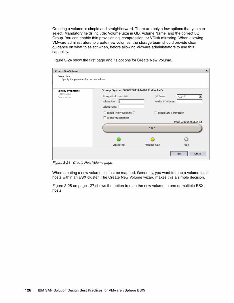
Creating a volume is simple and straightforward. There are only a few options that you can select. Mandatory fields include: Volume Size in GB, Volume Name, and the correct I/O Group. You can enable thin provisioning, compression, or VDisk mirroring. When allowing VMware administrators to create new volumes, the storage team should provide clear guidance on what to select when, before allowing VMware administrators to use this capability.

Figure 3-24 show the first page and its options for Create New Volume.

Figure 3-24 Create New Volume page

When creating a new volume, it must be mapped. Generally, you want to map a volume to all hosts within an ESX cluster. The Create New Volume wizard makes this a simple decision.

Figure 3-25 on page 127 shows the option to map the new volume to one or multiple ESX hosts.


Figure 3-25 LUN Mapping page

For the plug-in to work successfully, the SAN zoning to allow SAN communication between the VMware cluster and the storage system must already be completed. On the storage system, the ESX cluster and hosts definitions (representing the VMware cluster and its hosts) must have also been created. This process cannot be done from the plug-in, and is not done automatically. If the zoning and host definitions are not done, volume creation fails and the requested volume is created and then deleted.

Use the IBM Storage tab to identify the properties of the volume. The IBM Storage tab allows you to perform many useful storage tasks. From this tab, which is shown in Figure 3-26 on page 128, you can perform these tasks:

� Extend a volume. This task allows you to grow an existing volume and then later resize the datastore using that volume.

� Rename a volume. Use this task to ensure that the storage system volume name and the datastore name are the same. Having matching names on both sides will greatly improve manageability.

� Move a volume to a different pool on the storage system

� Confirm which datastore is which storage system volume.

� Confirm the status of all the volumes, snapshots, and mirrors. Mirrors cannot be confirmed if the user has read-only access.

� Confirm the size of the datastore in binary GiB and decimal GB.

� If the volume is not being used by a datastore, it can be unmapped and deleted. This process allows a VMware administrator to safely return a volume back to the storage system. Without the IBM Storage plug-in, this is a risky and complicated process. First, you need to delete the datastore from the VMware Datastore menu and then the volume

Tip: If you perform changes, such as renaming or resizing volumes, updates might take up to 60 seconds to display in the plug-in.


will show in the Unused LUNs tab and can be deleted using a right click and selecting the specific option.

Figure 3-26 shows the IBM Storage Plug-in Datastore Summary tab and the information that it provides.

Figure 3-26 IBM Storage Plug-in Datastore Summary tab

3.12.1 Conclusion

The IBM Storage Management Console for VMware vCenter plug-in is a great improvement for having an end-to-end view of your supported storage systems. If your organizational structure does not allow the VMware administrator to make storage administration decisions, you can still use the plug-in with read-only access. To do so, create a user on the IBM storage system that is in the Read Only category. When adding the IBM storage system to the IBM Storage plug-in, use this restricted Read Only user. The IBM Storage plug-in has to be installed on the same server as the vCenter Server because the vCenter Server appliance is currently not supported. This could be a reason not to use the IBM Storage Management Console for VMware vCenter plug-in. Another reason could be that your organization’s security policy does not allow an IP connection from the vCenter Server to the IBM storage system. However, if there are no technical or security constraints that prevent you from using this plug-in, there is no reason not to do so. Even in read only mode, it provides great help for the VMware administrator and can help to manage the environment as well as help troubleshooting.

3.13 General recommendation

As a general recommendation, we advise you to always check hardware compatibility. We cannot stress this enough but check features, hardware components, and the firmware level for compatibility in the VMware Compatibility Guide. It is not enough to verify that your hardware is supported. You need to go into the details to see in what configuration the


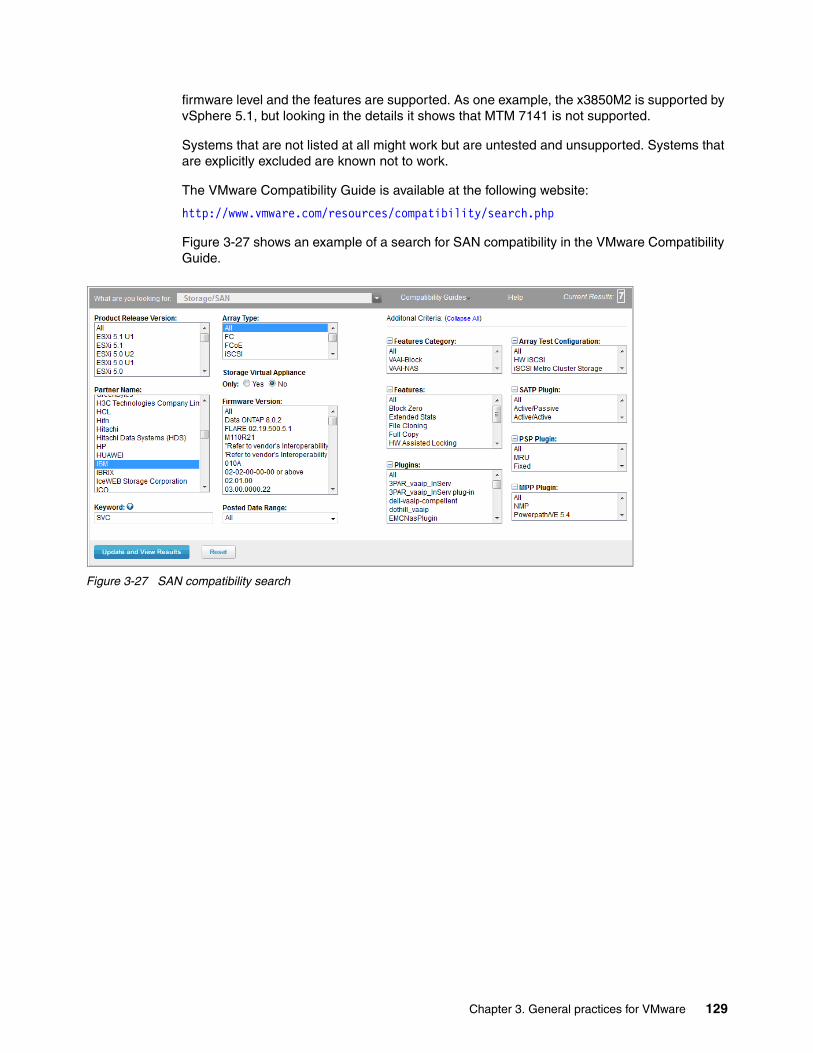
firmware level and the features are supported. As one example, the x3850M2 is supported by vSphere 5.1, but looking in the details it shows that MTM 7141 is not supported.

Systems that are not listed at all might work but are untested and unsupported. Systems that are explicitly excluded are known not to work.

The VMware Compatibility Guide is available at the following website:

http://www.vmware.com/resources/compatibility/search.php

Figure 3-27 shows an example of a search for SAN compatibility in the VMware Compatibility Guide.

Figure 3-27 SAN compatibility search




Figure 3-28 shows an example of a search result for SAN devices using the VMware Compatibility Guide.

Figure 3-28 Compatibility search result

Figure 3-29 on page 131 shows an example of the details for an SVC.


Figure 3-29 Compatibility details for an SVC

Ensure that you know the VMware maximums for the specific release. For very simple and small environments you probably do not hit any of the maxima, but the larger your environment gets the more important they get. Some are related and maybe not that obvious. For instance, you have a maximum of 1024 total paths per host and you have 256 LUNs per host. Now, if you have 8 instead of 4 paths, you end up with 128 because 1024/8 = 128. A recommendation is to zone all ESXi in a cluster identically so that all hosts should see the same LUNs. This means that 256 is not only the maximum for a host, but also for the cluster.

Also, the maximum means that it is a technical maximum or limitation. It does not necessarily mean that you can fully use the maximum. For instance, the maximum of virtual machines per host is 512. But this does not mean that you can run 512 virtual machines per host. Virtual CPUs per core are 25, and again you can set up that many virtual CPUs, but most likely they will not perform very well. If you have a test environment where most of the time no virtual machine is actually doing anything, this looks fine, but in a production environment it is probably not a good idea. The same applies for storage. For example, the maximum size of a single LUN (volume) is now 64 TB, but this does not mean that it is a good idea to use a 64 TB datastore. In most cases, it probably will not. Study the configuration maximums when planning your design.

For more information about configuration maximums for vSphere 5.1, see the following PDF document:

http://www.vmware.com/pdf/vsphere5/r51/vsphere-51-configuration-maximums.pdf




Chapter 4. General practices for storage

This chapter describes some general practices and recommendations for target storage devices. From disk to host, there are many factors to consider because every piece of the storage area network (SAN) has a part to play.

This chapter describes the following topics, from disk to host:

� General storage systems guidelines� Disks� MDisks and volumes� Back-end� Front end and fabric� Host

4


4.1 Configuring and servicing external storage systems

In this section, we provide some general guidelines for external storage systems that the SAN Volume Controller (SVC), Storwize V7000, and Storwize V3700 require for storage virtualization.

Both the Storwize V7000 and the Storwize V3700 are both stand-alone storage systems and storage virtualization devices. The Storwize V3700 can be used only in this capacity to migrate data to its internal disks.

4.1.1 General guidelines for SAN Volume Controller

Follow the guidelines and procedures for your storage system to maximize performance and to avoid potential I/O problems:

� Avoid splitting arrays into multiple logical disks at the storage system level. Where possible, create a single logical disk from the entire capacity of the array.

� Depending on the redundancy that is required, create RAID-5 (RAID 5) arrays by using 5 - 8 data bits plus parity components (that is, 5 + P, 6 + P, 7 + P, or 8 + P).

� Do not mix managed disks (MDisks) that greatly vary in performance in the same storage pool tier. The overall storage pool performance in a tier is limited by the slowest MDisk. Because some storage systems can sustain much higher I/O bandwidths than others, do not mix MDisks that are provided by low-end storage systems with those that are provided by high-end storage systems in the same tier. You must consider the following factors:

– The underlying Redundant Array of Independent Disks (RAID) type that the storage system is using to implement the MDisk.

– The number of physical disks in the array and the physical disk type (for example: 10,000 or 15,000 rpm, Fibre Channel, or Serial Advanced Technology Attachment (SATA)).

� When possible, include similarly sized MDisks in a storage pool tier. This makes it easier to balance the MDisks in the storage pool tier. If the MDisks in a storage pool tier are significantly different sizes, you can balance the proportion of space that is allocated on each MDisk by including the larger MDisk multiple times in the MDisk list. This is specified when you create a new volume. For example, if you have two 400 MB disks and one 800 MB disk that are identified as MDisk 0, 1, and 2, you can create the striped volume with the MDisk IDs of 0:1:2:2. This doubles the number of extents on the 800 MB drive, which accommodates it being double the size of the other MDisks.

� Perform the appropriate calculations to ensure that your storage systems are configured correctly.

If any storage system that is associated with an MDisk has the allowquorum parameter set to no, the chquorum command fails for that MDisk. Before setting the allowquorum parameter to yes on any storage system, check the following website for storage system configuration requirements:

http://www.ibm.com/storage/support/2145

4.1.2 General Guidelines for Storwize V7000

To avoid performance issues, you must ensure that your SAN-attached storage systems and switches are correctly configured to work efficiently with Storwize V7000 symmetric




virtualization. Before you create any volumes on external storage, be sure to review “Configuration guidelines for storage systems”.

Configuration guidelines for storage systemsYou must follow the guidelines and procedures for your storage system to maximize performance and to avoid potential I/O problems.

General guidelines� You must follow these general guidelines when configuring your storage systems.

� Avoid splitting arrays into multiple logical disks at the storage system level. Where possible, create a single logical disk from the entire capacity of the array.

� Depending on the redundancy that is required, create RAID-5 (RAID 5) arrays by using 5 - 8 data bits plus parity components (that is, 5 + P, 6 + P, 7 + P, or 8 + P).

� Do not mix MDisks that greatly vary in performance in the same storage pool tier. The overall storage pool performance in a tier is limited by the slowest MDisk. Because some storage systems can sustain much higher I/O bandwidths than others, do not mix MDisks that are provided by low-end storage systems with those that are provided by high-end storage systems in the same tier. You must consider the following factors:

– The underlying RAID type that the storage system is using to implement the MDisk.

– The number of physical disks in the array and the physical disk type (for example: 10,000 or 15,000 rpm, Fibre Channel, or SATA).

� When possible, include similarly sized MDisks in a storage pool tier. This makes it easier to balance the MDisks in the storage pool tier. If the MDisks in a storage pool tier are significantly different sizes, you can balance the proportion of space that is allocated on each MDisk by including the larger MDisk multiple times in the MDisk list. This is specified when you create a new volume. For example, if you have two 400 MB disks and one 800 MB disk that are identified as MDisk 0, 1, and 2, you can create the striped volume with the MDisk IDs of 0:1:2:2. This doubles the number of extents on the 800 MB drive, which accommodates it being double the size of the other MDisks.

� Perform the appropriate calculations to ensure that your storage systems are configured correctly.

� If any storage system that is associated with an MDisk has the allowquorum parameter set to no, the chquorum command fails for that MDisk. Before setting the allowquorum parameter to yes on any storage system, check the following website for storage system configuration requirements:

http://www.ibm.com/storage/support/storwize/v7000/

4.1.3 Configuring the Storwize V3700

Configuring and servicing external storage systemsTo avoid performance issues, you must ensure that your SAN-attached storage systems and switches are correctly configured to work efficiently with Storwize V3700.

A Storwize V3700 can connect to external storage systems only to migrate data to the Storwize V3700 internal storage. The Storwize V3700 requires an appropriate optional Host Interface Card (HIC) to communicate with storage systems that are attached to the same Fibre Channel SAN.

Virtualization provides many benefits over direct-attached or direct SAN-attached storage systems. However, virtualization is more susceptible to performance hot spots than

Chapter 4. General practices for storage 135

http://www.ibm.com/storage/support/storwize/v7000/

direct-attached storage. Hot spots can cause I/O errors on your hosts and can potentially cause a loss of access to data. For more information about the Storwise V3700, see the following Support website.

http://www.ibm.com/storage/support/storwize/v3700

4.1.4 Storwize family presets

The management graphical user interface (GUI) contains a series of preestablished configuration options called presets that use commonly used settings to quickly configure objects on the system.

Presets are available for creating volumes and FlashCopy mappings and for setting up RAID configuration.

The recommendation is to use the default behavior, or presets, of the GUI to configure storage.

In effect, it will create arrays/MDisks within the I/O group (an I/O group in this case is a control enclosure and its serial-attached SCSI (SAS)-attached expansion enclosures) and put them in their own storage pools for that I/O group that is based on drive class. All volumes created from that storage pool will be serviced/owned by the control enclosure for that I/O group. This minimizes forwarding of I/O between control enclosures.

If you take this option, we built in recommended configurations into the wizards to make things simple and easy.

Volume presetsIBM Storwize V7000 supports the following types of volume presets.

Table 4-1 shows volume presets and their uses.

Table 4-1 Volume presets and their uses

Preset Purpose

Generic Creates a striped volume of the specified size in the specified storage pool.

Thin provision Creates a thin-provisioned volume of the specified size with the autoexpand feature enabled in the specified storage pool. Sets the volume and the storage pool warning size to 80%. Only the specified percentage of the capacity of the volume is allocated to the volume at the time of creation. The default value is 2% of the volume capacity.

Mirror Creates a volume with two copies of the data in two storage pools to protect against storage pool failures.

Thin mirror Creates a volume with two thin-provisioned copies of the data in two storage pools to protect against storage pool failures. For details about how the thin-provisioned copies are configured, see the thin-provision preset information in this table.

Compressed Creates a thin-provisioned volume where data is compressed when it is written and stored on the volume. Only the specified percentage of the capacity of the volume is allocated to the volume at the time of creation. The default value is 2% of the volume capacity.Note: Storwize V7000 CF8 or later versions support compressed preset.




FlashCopy mapping presetsIn the management GUI, FlashCopy mappings include presets that can be used for test environments and backup solutions.

Table 4-2 shows FlashCopy presets.

Table 4-2 FlashCopy presets

RAID configuration presetsRAID configuration presets are used to configure all available drives based on recommended values for the RAID level and drive class. The system detects the installed hardware then recommends a configuration that uses all the drives to build arrays that are protected with the appropriate number of spare drives. Each preset has a specific goal for the number of drives per array, the number of spare drives to maintain redundancy, and whether the drives in the array are balanced across enclosure chains, thus protecting the array from enclosure failures.

Note: Storwize V3700 does not have a compressed preset.

Preset Purpose

Snapshot Creates a point-in-time view of the production data. The snapshot is not intended to be an independent copy but is used to maintain a view of the production data at the time that the snapshot is created.

This preset automatically creates a thin-provisioned target volume with 0% of the capacity allocated at the time of creation. The preset uses a FlashCopy mapping with 0% background copy so that only data written to the source or target is copied to the target volume.

Clone Creates an exact replica of the volume, which can be changed without affecting the original volume. After the copy operation completes, the mapping that was created by the preset is automatically deleted.

This preset automatically creates a volume with the same properties as the source volume and creates a FlashCopy mapping with a background copy rate of 50. The FlashCopy mapping is configured to automatically delete itself when the FlashCopy mapping reaches 100% completion.

Backup Creates a point-in-time replica of the production data. After the copy completes, the backup view can be refreshed from the production data, with minimal copying of data from the production volume to the backup volume.

This preset automatically creates a volume with the same properties as the source volume. The preset creates an incremental FlashCopy mapping with a background copy rate of 50.


Table 4-3 shows the presets that are used for solid-state drives (SSDs) for the Storwize V7000 system.

Table 4-3 SSD RAID preset

Table 4-4 shows RAID presets that are used for hard disk drives for the Storwize V7000 system.

Table 4-4 Storwize V7000 other RAID presets

Preset Purpose RAID level

Drives per array goal

Spare drive goal

SSD RAID 5

Protects against a single drive failure. Data and one strip of parity are striped across all array members.

5 8 1

SSD RAID 6

Protects against two drive failures. Data and two strips of parity are striped across all array members.

6 12 1

SSD RAID 10

Provides good performance and protects against at least one drive failure. All data is mirrored on two array members.

10 8 1

SSD RAID 0

Provides no protection against drive failures. Use only for temporary volumes.

0 8 0

SSD RAID 1

Mirrors data to provide good performance and protection against drive failure. The mirrored pairs are spread between storage pools to be used for the Easy Tier function.

1 2 1

Preset Purpose RAID level

Width goal

Spare goal

Chain balance

Basic RAID 5

Protects against a single drive failure. Data and one strip of parity are striped across all array members.

5 8 1 All drives in the array are from the same chain wherever possible.

Basic RAID 6

Protects against two drive failures. Data and two strips of parity are striped across all array members.


Basic RAID 10

Provides good performance and protects against at least one drive failure. All data is mirrored on two array members.


Balanced RAID 10

Provides good performance and protects against at least one drive or enclosure failure. All data is mirrored on two array members. The mirrors are balanced across the two enclosure chains.

10 8 1 Exactly half of the drives are from each chain.

RAID 0 Provides no protection against drive failures. Use only for temporary volumes.


Note: Storwize V3700 does not have a Balanced RAID 10 preset; therefore, the Chain balance column does not apply.


4.2 Disk

In this section, we describe the considerations that are disk-related. We describe everything from IOPS to LUN or volume creation and assignment.

4.2.1 Input/output operations per second

It is important to note that input/output operations per second (IOPS) is requests per second. IOPS is not an indication of throughput; however, throughput affects IOPS.

There are several resources available that describe IOPS in great detail and for specific applications.

This section summarizes IOPS.

Standard disk IOPSDisk IOPS varies by disk manufacturer as well as by disk application, such as a notebook hard disk drive versus an enterprise storage drive.

Table 4-5 Shows disk types that are matched with IOPS

Write penalty multiplierThe write penalty multiplier is the number of I/Os per write request.

Table 4-6 Shows the RAID type and the associated write penalty multiplier

For example, with RAID 5 the write penalty is x4. What this means is that the storage controller initiates two read requests and two write requests with one of each for data and parity. In other words, one write means one read from the block that is going to be written to, and one read from parity in order to calculate the new parity. Then, there is one write for the data and one write for the newly calculated parity.

Spindle speed IOPS

5400 50 - 80

7200 75 - 100

10000 125 - 150

15000 175 - 210

SSD up to 2600

Tip: 5400 rpm hard disk drives are included only as a reference point. Most enterprise storage systems no longer use 5400 rpm drives.

RAID type Write penalty

RAID 0 x1

RAID 1,1/0, 0+1 x2

RAID 5 x4

RAID 6 x6


Calculating IOPSTo calculate basic IOPS, use the formula shown in this section. This shows an IOPS formula used to calculate the number of disks that are needed based on the requested IOPS, disk IOPS, and the write penalty multiplier.

Following is the IOPS formula:

Number of disks = (Requested IOPS x (Read percentage + Write percentage x RAID Factor))/Individual disk IOPS

As an example, a VMware administrator requests a LUN. IOPS is estimated to be 1000 with a 60/40 read/write ratio on tier 1 storage:

1. Number of disks = (1000 x (60% + 40% x 4))/1802. Number of disks = (1000 x (.6 + 0.4 x 4))/1803. Number of disks = (1000 x (.6 + 1.6))/1804. Number of disks = (1000 x (2.2))/1805. Number of disks = 2200/1806. Number of disks = 12.2 rounded up to 13

Because we always want to balance the number of disks that are used with the capacity used, we also want to compare different RAID levels. Using the same formula with a RAID factor of 2 provides eight disks for RAID 10.

For more in-depth information regarding IOPS, see the following website:

http://www.symantec.com/connect/articles/getting-hang-iops-v13

4.2.2 Disk types

There are several disk types that are available for use in today’s storage arrays from low speed, low-power archive disks, to SSD. Low speed drives are typically SATA technology, though recently, nearline SAS has emerged. There is also Fibre Channel and SAS for higher speed drives.

Today’s storage arrays are moving to SAS back-end to include nearline SAS. SAS is a more cost-effective solution because it does not require any additional Fibre Channel hardware on the hard disk drives, and it also offers multiple lanes of communication for more throughput. For example, a 6 Gbps SAS with four lanes has a theoretical maximum throughput of 600 MBps per lane for a total of 2400 MBps.

The Storwize V3700, Storwize V7000, and the SVC use SAS for their internal drives. External storage connections are performed through Fibre Channel zoning.

Note: Higher speed drives that connect through either a Fibre Channel or SAS interface, include 10,000 rpm, 15,000 rpm, and SSD.

Note: Nearline SAS is used to connect SATA drives to a SAS interface. These include both 5,400 rpm and 7,200 rpm drives.


http://www.symantec.com/connect/articles/getting-hang-iops-v13

4.3 MDisks and volumes

The following section describes matters that are related to MDisks and volumes.

4.3.1 Disk tiering

Disk tiering is the automated movement of logical units from one disk technology to another. This is usually done based on a combination of the frequency of access and IOPS.

For the SVC, disk tiering now includes Tier 0 for SSD. Table 4-7 shows general tier level to disk mapping recommendations.

Table 4-7 General tier level to disk mapping

Table 4-8 shows general tier level to RAID level mapping guidelines.

Table 4-8 General tier level to RAID level mapping

The SAN Volume Controller makes it easy to configure multiple tiers of storage within the same SVC cluster. You might have single-tiered pools, multi-tiered storage pools, or both.

In a single-tiered storage pool, the MDisks must have the following characteristics to avoid inducing performance problems and other issues:

� They have the same hardware characteristics, for example, the same RAID type, RAID array size, disk type, and disk revolutions per minute (rpm).

� The disk subsystems that provide the MDisks must have similar characteristics, for example, maximum IOPS, response time, cache, and throughput.

� The MDisks that are used are of the same size and are, therefore, MDisks that provide the same number of extents. If that is not feasible, you must check the distribution of the extents of the volumes in that storage pool.

Tip: This section applies to both the SAN Volume Controller and the Storwize V7000.

Tier level Disk type

Tier 0 SSD

Tier 1 15 K rpm

Tier 2 10 K rpm

Tier 3 7.2 K rpm

Tier level RAID level

Tier 1 RAID 10

Tier 2 RAID 5

Tier 3 RAID 6

Tip: With SSD, RAID 5 is recommended.


In a multi-tiered storage pool, you have a mix of MDisks with more than one type of disk tier attribute. For example, a storage pool contains a mix of generic_hdd and generic_ssd MDisks.

A multi-tiered storage pool, therefore, contains MDisks with various characteristics, as opposed to a single-tier storage pool. However, each tier must have MDisks of the same size and MDisks that provide the same number of extents. Multi-tiered storage pools are used to enable the automatic migration of extents between disk tiers by using the SAN Volume Controller Easy Tier function. For more information about IBM System Storage Easy Tier, see Chapter 11 of IBM System Storage SAN Volume Controller Best Practices and Performance Guidelines, SG24-7521.

http://www.redbooks.ibm.com/redbooks/pdfs/sg247521.pdf

It is likely that the MDisks (LUNs) that are presented to the SVC cluster have various performance attributes due to the type of disk or RAID array on which they reside. The MDisks can be on a 15 K rpm Fibre Channel (FC) or serial-attached SCSI (SAS) disk, a nearline SAS, or Serial Advanced Technology Attachment (SATA), or on SSDs. Therefore, a storage tier attribute is assigned to each MDisk, with the default of generic_hdd. With SAN Volume Controller V6.2, a new tier 0 (zero) level disk attribute is available for SSDs, and it is known as generic_ssd.

You can also define storage tiers by using storage controllers of varying performance and availability levels. Then, you can easily provision them based on host, application, and user requirements.

Remember that a single storage tier can be represented by multiple storage pools. For example, if you have a large pool of tier 3 storage that is provided by many low-cost storage controllers, it is sensible to use several storage pools. Usage of several storage pools prevents a single offline volume from taking all of the tier 3 storage offline.

When multiple storage tiers are defined, take precautions to ensure that storage is provisioned from the appropriate tiers. You can ensure that storage is provisioned from the appropriate tiers through storage pool and MDisk naming conventions, with clearly defined storage requirements for all hosts within the installation.

You can use the SAN Volume Controller to create tiers of storage, in which each tier has different performance characteristics, by including only managed disks (MDisks) that have the same performance characteristics within a managed disk group. Therefore, if you have a storage infrastructure with, for example, three classes of storage, you create each volume from the managed disk group that has the class of storage that most closely matches the expected performance characteristics of the volume.

Because migrating between storage pools, or rather managed disk groups, is nondisruptive to users, it is easy to migrate a volume to another storage pool if the performance is different than expected.

Naming conventions: When multiple tiers are configured, clearly indicate the storage tier in the naming convention that is used for the storage pools and MDisks.

Tip: If you are uncertain about in which storage pool to create a volume, initially use the pool with the lowest performance and then move the volume up to a higher performing pool later if required.




4.3.2 Logical disk configuration guidelines for storage systems

Most storage systems provide some mechanism to create multiple logical disks from a single array. This is useful when the storage system presents storage directly to the hosts.

However, in a virtualized SAN, use a one-to-one mapping between arrays and logical disks so that the subsequent load calculations and the MDisk and storage pool configuration tasks are simplified.

Scenario: the logical disks are unevenIn this example scenario, you have two RAID-5 arrays and both contain 5 + P components. Array A has a single logical disk that is presented to the SAN Volume Controller clustered system. This logical disk is seen by the system as MDisk0. Array B has three logical disks that are presented to the system. These logical disks are seen by the system as MDisk1, MDisk2, and MDisk3. All four MDisks are assigned to the same storage pool that is named MDisk_grp0. When a volume is created by striping across this storage pool, array A presents the first extent and array B presents the next three extents. As a result, when the system reads and writes to the volume, the loading is split 25% on the disks in array A and 75% on the disks in array B. The performance of the volume is about one-third of what array B can sustain.

The uneven logical disks cause performance degradation and complexity in a simple configuration. You can avoid uneven logical disks by creating a single logical disk from each array.

Figure 4-1 shows an uneven logical disk layout.

Figure 4-1 Uneven logical disk layout

4.3.3 RAID configuration guidelines for storage systems

With virtualization, ensure that the storage devices are configured to provide some type of redundancy against hard disk failures.


A failure of a storage device can affect a larger amount of storage that is presented to the hosts. To provide redundancy, storage devices can be configured as arrays that use either mirroring or parity to protect against single failures.

When creating arrays with parity protection (for example, RAID-5 arrays), consider how many component disks you want to use in each array. If you use a large number of disks, you can reduce the number of disks that are required to provide availability for the same total capacity (1 per array). However, more disks mean that it takes a longer time to rebuild a replacement disk after a disk failure, and during this period a second disk failure causes a loss of all array data. More data is affected by a disk failure for a larger number of member disks because performance is reduced while you rebuild onto a hot spare (a redundant disk) and more data is exposed if a second disk fails before the rebuild operation is complete. The smaller the number of disks, the more likely it is that write operations span an entire stripe (stripe size, multiplied by the number of members, minus one). In this case, write performance is improved. The number of disk drives required to provide availability can be unacceptable if arrays are too small.

4.3.4 Optimal storage pool configuration guidelines for storage systems

A storage pool provides the pool of storage from which volumes are created. You must ensure that the MDisks that make up each tier of the storage pool have the same performance and reliability characteristics.

Consider the following factors:

� The performance of a storage pool is generally governed by the slowest MDisk in the storage pool.

� The reliability of a storage pool is generally governed by the weakest MDisk in the storage pool.

� If a single MDisk in a group fails, access to the entire group is lost.

Use the following guidelines when you group similar disks:

� Group equally performing MDisks in a single tier of a pool.

� Group similar arrays in a single tier. For example, configure all 6 + P RAID-5 arrays in one tier of a pool.

� Group MDisks from the same type of storage system in a single tier of a pool.

� Group MDisks that use the same type of underlying physical disk in a single tier of a pool. For example, group MDisks by Fibre Channel or SATA.

� Do not use single disks. Single disks do not provide redundancy. Failure of a single disk results in total data loss of the storage pool to which it is assigned.

Note: Consider the following factors:

� For optimal performance, use arrays with 6 - 8 member disks.

� When creating arrays with mirroring, the number of component disks in each array does not affect redundancy or performance.


Scenario: similar disks are not grouped togetherUnder one scenario, you could have two storage systems that are attached behind your SAN Volume Controller. For example, one device contains ten 6 + P RAID-5 arrays and MDisks 0 - 9. The other device contains a single RAID-1 array, MDisk10, one single just a bunch of disks (JBOD), MDisk11, and a large 15 + P RAID-5 array, MDisk12.

If you assigned MDisks 0 - 9 and MDisk11 into a single storage pool, and the JBOD MDisk11 fails, you lose access to all of those arrays, even though they are online.

To fix this problem, you can create three groups. The first group must contain the MDisks 0 - 9, the second group must contain the RAID 1 array, and the third group must contain the large RAID 5 array.

Figure 4-2 shows dissimilar disk groups.

Figure 4-2 Dissimilar disk groups

If MDisk 11 loses a signal drive, the access is lost to the entire MDisk group.

4.3.5 FlashCopy mapping guidelines for storage systems

Ensure that you have considered the type of I/O and frequency of update before you create the volumes that you want to use in FlashCopy mappings.

FlashCopy operations perform in direct proportion to the performance of the source and target disks. If you have a fast source disk and slow target disk, the performance of the source


disk is reduced because it has to wait for the write operation to occur at the target before it can write to the source.

The FlashCopy implementation that is provided by the SAN Volume Controller copies at least 256 K every time a write is made to the source. This means that any write involves at minimum a read of 256 K from the source, write of the same 256 K at the target, and a write of the original change at the target. Therefore, when an application performs small 4 K writes, this is translated into 256 K.

Because of this overhead, consider the type of I/O that your application performs during a FlashCopy operation. Ensure that you do not overload the storage. The calculations contain a heavy weighting when the FlashCopy feature is active. The weighting depends on the type of I/O that is performed. Random writes have a much higher overhead than sequential writes. For example, the sequential write would have copied the entire 256 K.

You can spread the FlashCopy source volumes and the FlashCopy target volumes between as many MDisk groups as possible. This limits the potential bottle-necking of a single storage system (assuming that the storage pools contain MDisks from different storage systems). However, this can still result in potential bottlenecks if you want to maintain all your target volumes on a single storage system. You must ensure that you add the appropriate weighting to your calculations.

4.3.6 Image mode volumes and data migration guidelines for storage systems

Image mode volumes enable you to import and then migrate existing data that is managed by an external storage system into the SAN Volume Controller.

Ensure that you follow the guidelines for using image mode volumes. This might be difficult because a configuration of logical disks and arrays that performs well in a direct SAN-attached environment can contain hot spots or hot component disks when they are connected through the clustered system.

If the existing storage systems do not follow the configuration guidelines, consider completing the data migration away from the image mode volume before resuming I/O operations on the host systems. If I/O operations are continued and the storage system does not follow the guidelines, I/O operations can fail at the hosts and ultimately loss of access to the data can occur.

The procedure for importing MDisks that contain existing data depends on the amount of free capacity that you have in the system. You must have the same amount of free space in the system as the size of the data that you want to migrate into the system. If you do not have this amount of available capacity, the migration causes the storage pool to have an uneven distribution of data because some MDisks are more heavily loaded than others. Further migration operations are required to ensure an even distribution of data and subsequent I/O loading.

Importing image mode volumes with an equivalent amount of free capacityWhen importing an image mode volume that has a certain amount of gigabytes and your system has at least that amount in a single storage pool, follow the Start New Migration

Attention: Migration commands fail if the target or source volume is offline, or if there is insufficient quorum disk space to store the metadata. Correct the offline or quorum disk condition and reissue the command.


wizard in the management GUI at Physical Storage Migration to import the image mode volumes and to provide an even distribution of data.

Importing image mode volumes with a smaller amount of free capacityWhen importing an image mode, volume that has a certain amount of gigabytes, and your system does not have at least that amount of free capacity in a single storage pool, follow the Start New Migration wizard in the management GUI at Physical Storage Migration to import the image mode volumes. Do not select the destination pool at the end of the wizard. This will cause the system to create the image mode volumes but does not migrate the data away from the image mode volumes. Use volume mirroring or migration to move the data around as you want.

4.3.7 Configuring a balanced storage system

The attachment of a storage system to a SAN Volume Controller requires that specific settings are applied to the device.

There are two major steps to attaching a storage system to a SAN Volume Controller:

� Setting the characteristics of the SAN Volume Controller to storage connections� Mapping logical units to these storage connections that allow the SAN Volume Controller

to access the logical units

The virtualization features of the SAN Volume Controller enable you to choose how your storage is divided and presented to hosts. Although virtualization provides you with a great deal of flexibility, it also offers the potential to set up an overloaded storage system. A storage system is overloaded if the quantity of I/O transactions that are issued by the host systems exceed the capability of the storage to process those transactions. If a storage system is overloaded, it causes delays on the host systems and might cause I/O transactions to time out on the host. If I/O transactions time out, the host logs errors and I/Os fail to the applications.

Scenario: an overloaded storage systemIn this scenario, assume that you have used the SAN Volume Controller system to virtualize a single array and to divide the storage across 64 host systems. If all host systems attempt to access the storage at the same time, the single array is overloaded.

Perform the following steps to configure a balanced storage system:

Procedure1. Use Table 4-9 to calculate the I/O rate for each RAID in the storage system.

Table 4-9 shows how to calculate the I/O rate.

Table 4-9 Calculate the I/O rate

Note: The actual number of IOPS that can be processed depends on the location and length of each I/O, whether the I/O is a read or a write operation, and on the specifications of the component disks of the array. For example, a RAID-5 array with eight component disks has an approximate I/O rate of 150 × 7=1050.

Type of array Number of component disks in the array

Approximate I/O rate per second

RAID-1 (mirrored) arrays 2 300


2. Calculate the I/O rate for an MDisk.

– If there is a one-to-one relationship between back-end arrays and MDisks, the I/O rate for an MDisk is the same as the I/O rate of the corresponding array.

– If an array is divided into multiple MDisks, the I/O rate per MDisk is the I/O rate of the array divided by the number of MDisks that are using the array.

3. Calculate the I/O rate for a storage pool. The I/O rate for a storage pool is the sum of the I/O rates of the MDisk that is in the storage pool. For example, a storage pool contains eight MDisks and each MDisk corresponds to a RAID-1 array. Using Table 4-9 on page 147, the I/O rate for each MDisk is calculated as 300. The I/O rate for the storage pool is 300 × 8 = 2400.

4. Use Table 4-10 to calculate the impact of FlashCopy mappings. If you are using the FlashCopy feature that is provided by the SAN Volume Controller, you must consider the additional amount of I/O that FlashCopy operations generate because it reduces the rate at which I/O from host systems can be processed. When a FlashCopy mapping copies write I/Os from the host systems to areas of the source or target volume that are not yet copied, the SAN Volume Controller generates extra I/Os to copy the data before the write I/O is performed. The effect of using the FlashCopy feature depends on the type of I/O workload that is generated by an application.

Table 4-10 shows how to calculate the impact of FlashCopy mappings.

Table 4-10 Calculate the impact of FlashCopy mappings

For each volume that is the source or target of an active FlashCopy mapping, consider the type of application that you want to use for the volume and record the additional weighting for the volume.

ExamplesFor example, a FlashCopy mapping is used to provide point-in-time backups. During the FlashCopy process, a host application generates an I/O workload of random read and write operations to the source volume. A second host application reads the target volume and writes the data to tape to create a backup. The additional weighting for the source volume is 14. The additional weighting for the target volume is 0.

RAID-3, RAID-4, RAID-5 (striped + parity) arrays

N + 1 parity 150 x N

RAID-10, RAID 0+1, RAID 1+0 (striped + mirrored) arrays

N 150 x N

Type of application Impact to I/O rate Additional weighting for FlashCopy

Application is not performing I/O Insignificant impact 0

Application is only reading data Insignificant impact 0

Application is only issuing random writes Up to 50 times as much I/O 49

Application is issuing random reads and writes Up to 15 times as much I/O 14

Application is issuing sequential reads or writes Up to 2 times as much I/O 1

Type of array Number of component disks in the array

Approximate I/O rate per second


5. Calculate the I/O rate for volumes in a storage pool by performing the following steps:

a. Calculate the number of volumes in the storage pool.

b. Add the additional weighting for each volume that is the source or target of an active FlashCopy mapping.

c. Divide the I/O rate of the storage pool by this number to calculate the I/O rate per volume.

Example 1A storage pool has an I/O rate of 2400 and contains 20 volumes. There are no FlashCopy mappings. The I/O rate per volume is 2400 / 20 = 120.

Example 2A storage pool has an I/O rate of 5000 and contains 20 volumes. There are two active FlashCopy mappings that have source volumes in the storage pool. Both source volumes are accessed by applications that issue random read and write operations. As a result, the additional weighting for each volume is 14. The I/O rate per volume is 5000 / (20 + 14 + 14) = 104.

6. Determine if the storage system is overloaded. The figure that was determined in step 4 provides some indication of how many I/O operations per second can be processed by each volume in the storage pool.

� If you know how many I/O operations per second that your host applications generate, you can compare these figures to determine if the system is overloaded.

� If you do not know how many I/O operations per second that your host applications generate, you can use the I/O statistics facilities that are provided by the SAN Volume Controller to measure the I/O rate of your volumes, or you can use Table 4-11 as a guideline.

Table 4-11 shows how to determine if the storage system is overloaded.

Table 4-11 Determine if the storage system is overloaded

7. Interpret the result. If the I/O rate that is generated by the application exceeds the I/O rate per volume that you calculated, you might be overloading your storage system. You must carefully monitor the storage system to determine if the back-end storage limits the overall performance of the storage system. It is also possible that the previous calculation is too

Note: Step 5 is a continuation from Step 4 on page 148.

Note: Step 6 is a continuation from Step 5.

Type of application I/O rate per volume

Applications that generate a high I/O workload 200

Applications that generate a medium I/O workload 80

Applications that generate a low I/O workload 10

Note: Step 7 is a continuation from Step 6.


simplistic to model your storage use after. For example, the calculation assumes that your applications generate the same I/O workload to all volumes, which might not be the case.

You can use the I/O statistics facilities that are provided by the SAN Volume Controller to measure the I/O rate of your MDisks. You can also use the performance and I/O statistics’ facilities that are provided by your storage systems.

What to do nextIf your storage system is overloaded, there are several actions that you can take to resolve the problem:

� Add more back-end storage to the system to increase the quantity of I/O that can be processed by the storage system. The SAN Volume Controller provides virtualization and data migration facilities to redistribute the I/O workload of volumes across a greater number of MDisks without having to take the storage offline.

� Stop unnecessary FlashCopy mappings to reduce the number of I/O operations that are submitted to the back-end storage. If you perform FlashCopy operations in parallel, consider reducing the number of FlashCopy mappings that start in parallel.

� Adjust the queue depth to limit the I/O workload that is generated by a host. Depending on the type of host and type of host bus adapters (HBAs), it might be possible to limit the queue depth per volume or limit the queue depth per HBA, or both. The SAN Volume Controller also provides I/O governing features that can limit the I/O workload that is generated by hosts.

To configure specific storage systems, see the following sites for each storage device:

Storwize V3700:

http://pic.dhe.ibm.com/infocenter/storwize/v3700_ic/index.jsp

Storwize V7000:

http://pic.dhe.ibm.com/infocenter/storwize/ic/index.jsp

SAN Volume Controller:


4.4 Volumes

In this section, we describe matters that are related to volumes.

4.4.1 Thin provisioning

Volumes can be configured as thin-provisioned or fully allocated. Thin-provisioned volumes are created with real and virtual capacities. You can still create volumes by using a striped, sequential, or image mode virtualization policy, just as you can with any other volume.

Real capacity defines how much disk space is allocated to a volume. Virtual capacity is the capacity of the volume that is reported to other IBM System Storage SAN Volume Controller (SVC) components (such as FlashCopy or remote copy) and to the hosts.

Note: Although these actions can be used to avoid I/O timeouts, performance of your storage system is still limited by the amount of storage that you have.



http://pic.dhe.ibm.com/infocenter/storwize/ic/index.jsp




A directory maps the virtual address space to the real address space. The directory and the user data share the real capacity.

Thin-provisioned volumes come in two operating modes: autoexpand and nonautoexpand. You can switch the mode at any time. If you select the autoexpand feature, the SVC automatically adds a fixed amount of additional real capacity to the thin volume as required. Therefore, the autoexpand feature attempts to maintain a fixed amount of unused real capacity for the volume. This amount is known as the contingency capacity. The contingency capacity is initially set to the real capacity that is assigned when the volume is created. If the user modifies the real capacity, the contingency capacity is reset to be the difference between the used capacity and real capacity.

A volume that is created without the autoexpand feature, and thus has a zero contingency capacity, goes offline as soon as the real capacity is used and needs to expand.

Autoexpand mode does not cause real capacity to grow much beyond the virtual capacity. The real capacity can be manually expanded to more than the maximum that is required by the current virtual capacity, and the contingency capacity is recalculated.

A thin-provisioned volume can be converted non-disruptively to a fully allocated volume, or vice versa, by using the volume mirroring function. For example, you can add a thin-provisioned copy to a fully allocated primary volume and then remove the fully allocated copy from the volume after they are synchronized.

The fully allocated to thin-provisioned migration procedure uses a zero-detection algorithm so that grains that contain all zeros do not cause any real capacity to be used.

Space allocationWhen a thin-provisioned volume is initially created, a small amount of the real capacity is used for initial metadata. Write I/Os to the grains of the thin volume (that were not previously written to) cause grains of the real capacity to be used to store metadata and user data. Write I/Os to the grains (that were previously written to) update the grain where data was previously written.

Smaller granularities can save more space, but they have larger directories. When you use thin-provisioning with FlashCopy, specify the same grain size for both the thin-provisioned volume and FlashCopy.

Thin-provisioned volume performanceThin-provisioned volumes require more I/Os because of the directory accesses:

� For truly random workloads, a thin-provisioned volume requires approximately one directory I/O for every user I/O so that performance is 50% of a normal volume.

Warning threshold: Enable the warning threshold (by using email or an SNMP trap) when working with thin-provisioned volumes, on the volume, and on the storage pool side, especially when you do not use the autoexpand mode. Otherwise, the thin volume goes offline if it runs out of space.

Tip: Consider using thin-provisioned volumes as targets in FlashCopy relationships.

Grain definition: The grain is defined when the volume is created and can be 32 KB, 64 KB, 128 KB, or 256 KB.


� The directory is two-way write-back cache (similar to the SVC fastwrite cache) so that certain applications perform better.

� Thin-provisioned volumes require more CPU processing so that the performance per I/O group is lower.

Use the striping policy to spread thin-provisioned volumes across many storage pools.

Thin-provisioned volumes save capacity only if the host server does not write to whole volumes. Whether the thin-provisioned volume works well partly depends on how the file system allocated the space:

� Some file systems (for example, New Technology File System (NTFS)) write to the whole volume before they overwrite the deleted files. Other file systems reuse space in preference to allocating new space.

� File system problems can be moderated by tools, such as “defrag,” or by managing storage by using host Logical Volume Managers (LVMs).

The thin-provisioned volume also depends on how applications use the file system. For example, some applications delete log files only when the file system is nearly full.

There is no recommendation for thin-provisioned volumes. As explained previously, the performance of thin-provisioned volumes depends on what is used in the particular environment. For the absolute best performance, use fully allocated volumes instead of a thin-provisioned volume.

Limits on virtual capacity of thin-provisioned volumesA couple of factors (extent and grain size) limits the virtual capacity of thin-provisioned volumes beyond the factors that limit the capacity of regular volumes. Table 4-12 shows the maximum thin-provisioned volume virtual capacities for an extent size.

Table 4-12 Maximum thin volume virtual capacities for an extent size

Important: Do not use thin-provisioned volumes where high I/O performance is required.

Extent size in MB Maximum volume real capacity in GB

Maximum thin virtual capacityin GB

16 2,048 2,000

32 4,096 4,000

64 8,192 8,000

128 16,384 16,000

256 32,768 32,000

512 65,536 65,000

1024 131,072 130,000

2048 262,144 260,000

4096 524,288 520,000

8192 1,048,576 1,040,000


Table 4-13 shows the maximum thin-provisioned volume virtual capacities for a grain size.

Table 4-13 Maximum thin volume virtual capacities for a grain size

4.5 Back-end

The back-end section is the connection from the storage controller to the disks. In most Active/Passive arrays, this is split between two controllers. In most Active/Active arrays, the back-end can span several controllers.

The SVC, Storwize V7000, and Storwize V3700 are all Active/Active storage arrays.

It can be said that virtualized storage is double back-ended. There is the back-end of the controller (SVC, Storwize V7000, Storwize V3700) and there is the back-end of any external storage devices that are virtualized by the SVC, Storwize V7000, or Storwize V3700.

4.6 Front-end/fabric

The front-end is the connection from the storage controller to the host.

VMware is very sensitive to Host/LUN Pathing. Each path from ESX to the storage is treated as one LUN by ESX. If you have eight paths zoned, 1 LUN from the storage array is 8 LUNs on ESX. This is important because ESX has a hard limit of 1024 LUNs.

In Figure 4-6 on page 155, it is possible to have a total of 16 paths from each server. With 16 paths, ESX is hard limited to 64 total LUNs.

For front-end connections to the Storwize V7000, we start with a physical connection drawing and we progress down to a logical connection view. What we have done here is split the hosts at the front-end. Host A will be logically connected to half of the ports and Host B will be logically connected to the other half of the ports.

Grain size in KB Maximum thin virtual capacity in GB

32 260,000

64 520,000

128 1,040,000

256 2,080,000

Pathing versus Multipathing:

Pathing refers to a single path or zoning. Pathing can also refer to individual links to storage.

Multipathing refers to the intermediary driver that handles merging a LUN that is presented from a storage device down multiple paths to a single usable LUN by a host.


Figure 4-3 shows dual fabric physical cabling.

Figure 4-3 Dual fabric physical cabling

In this physical connection diagram, we have two hosts connected to two fabrics connected to a single Storwize V7000.

With this cabling scheme, it is possible to have 8-way multipathing.

In Figure 4-4 and Figure 4-5 on page 155, we show how we can split host A and host B up so that only four paths are presented to ESX, and how to balance the front-end ports.

Figure 4-4 shows Host A logical connections.

Figure 4-4 Host A logical connections

Host A’s logical connections are set as the following:

� HBA1_Canister1_Port4� HBA1_Canister2_Port3� HBA2_Canister1_Port1� HBA2_Canister2_Port2

Figure 4-5 on page 155 shows Host B logical connections.


Figure 4-5 Host B logical connections

Host B’s logical connections are set as per the following:

� HBA1_Canister1_Port2� HBA1_Canister2_Port1� HBA2_Canister1_Port3� HBA2_Canister2_Port4

Host A’s connections are exactly the opposite of Host B’s connections on the storage device. This allows us to balance the storage devices’ front-end ports.

4.6.1 4-way multipathing

If you have a single server with two dual port Fibre Channel HBAs installed that are connected to two separate fabrics, which are connected to a quad port dual storage head, you have a total of 16 paths available. Having this many physical connections is a good thing. Having this many logical connections is not good when you are up against a host LUN count limit, such as VMware.

In order to maximize redundancy with multipathing, we recommend 4-way multipathing.

Figure 4-6 shows 16 total available paths.

Figure 4-6 16 total paths

Important: In some cases, maximum pathing (or zoning) is required. If this is the case, limiting the host/LUN path count will need to be done on the storage controllers. For SVC, this is called a pseudohost.


Figure 4-7 shows a 4-way multipathing scheme.

Figure 4-7 4-way multipathing scheme

In order to balance the front-end ports of the Storwize V7000, the next host should be connected as shown in Figure 4-8.

Figure 4-8 shows 4-way multipathing with a second host.

Figure 4-8 4-way multipathing with a second host

There are two canister slots, one above the other, in the middle of the chassis. The top slot is canister 1. The bottom slot is canister 2. The canisters are inserted different ways up. Canister 1 appears the correct way up, and canister 2 upside down.

Table 4-14 shows the physical canister front-end port layout of the Storwize V7000.

Table 4-14 Storwize V7000 canister front-end port layout

Zones:

� HBA1_Canister1_Port4� HBA1_Canister2_Port3

Canister 1 Canister 2

1 2 3 4

3 4 2 1


� HBA2_Canister1_Port1� HBA2_Canister2_Port2

In this zoning/cabling configuration, we are storage redundant (Controller A and Controller B), we are controller-port redundant (A0 and A1, B0 and B1), we are fabric redundant (Fabric A and Fabric B), and we are HBA redundant (HBA0 and HBA1). (4-way redundancy).

Each HBA has a path to both controllers, but not to every FE port.

Below are the various faults that can occur:

� If HBA1 fails, HBA2 still has access to both controllers. The LUN should not move. At this point, we are storage redundant only. (1 way)

� If HBA2 fails, HBA1 still has access to both controllers. The LUN should not move. At this point, we are storage redundant only. (1 way)

� If Fabric A fails, Fabric B still has access to both controllers. The LUN should not move. At this point, we are storage redundant only. (1 way)

� If Fabric B fails, Fabric A still has access to both controllers. The LUN should not move. At this point, we are storage redundant only. (1 way)

� If Controller A fails, both HBAs and fabrics still have access to Controller B. All LUNs owned by Controller A should trespass to Controller B. Primary HBA access should not change because the LUNs should be presented through the secondary (one) port. This is fabric and host redundant. (2 way)

� If Controller B fails, both HBAs and fabrics still have access to Controller A. All LUNs owned by Controller B should trespass to Controller A. Primary HBA access should not change because the LUNs should be presented through the secondary (one) port. This is fabric and host redundant. (2 way)

� If a target N_Port on any switch fails, both HBAs and both fabrics still have access to both controllers. LUN access (from the host perspective only) can change, but should not trespass, depending on the multipathing software in use. This is still considered to be storage, host, and fabric redundant. This is not controller-port redundant. (3 way)

An initiator N_Port fault is congruent to an HBA fault. (1 way)

� If any target port on any of the storage controllers fails, both HBAs and both fabrics still have access to both controllers. LUN access can change, but should not trespass as above. This is still considered to be storage, host, and fabric redundant. This is not controller-port redundant. (3 way)

In all of the above scenarios, host/LUN pathing may change. If a host is split between controllers, half the pathing will change at the host level.

4.6.2 8-way multipathing

Building on the 4-way multipathing scheme above, this is an example of an 8-way multipathing scheme.

Tip: A target N_Port is a storage device port.

Tip: An initiator N_Port is usually an HBA port, but not always. An initiator can also be a target.


Figure 4-9 shows an 8-way multipathing scheme.


Following are the zones for an 8-way multipathing scheme:

� HBA1_Port0_Canister1_Port4� HBA1_Port0_Canister2_Port3� HBA1_Port1_Canister1_Port1� HBA1_Port1_Canister2_Port2� HBA2_Port0_Canister1_Port1� HBA2_Port0_Canister2_Port3� HBA2_Port1_Canister1_Port4� HBA2_Port1_Canister2_Port2

In this zoning/cabling configuration, we are storage redundant (Controller A and Controller B), we are controller-port redundant (A0 and A1, B0 and B1), we are fabric redundant (Fabric A and Fabric B), we are HBA redundant (HBA1 and HBA2), and we are HBA port redundant (HBA Port0 and Port1) giving us 5-way redundancy.

Multipathing is set to a default of failover or failback.

Both HBAs have paths to both controller primary ports (zeros) and failover secondary ports (ones). In other words, both HBAs have a connection to every FE port.

Following are the various faults that could possibly occur.

� If HBA 1 fails, HBA 2 still has access to every FE port from both fabrics. The LUN should not move. Host LUN access may change. This is now storage, FE port, HBA port, and fabric redundant. (4 way)

Note: In Figure 4-9, note that half of the front-end ports are used. To connect a second host, zone to the unused ports and alternate with every host attached.

Tip: Notice that Canisterx_Porty is repeated twice.

Example:

� HBA1_Port1_Canister1_Port1� HBA2_Port0_Canister1_Port1


� If HBA 2 fails, HBA 1 still has access to every FE port from both fabrics. The LUN should not move. Host LUN access may change. This is now storage, FE port, HBA port, and fabric redundant. (4 way)

� If Fabric A fails, both HBAs still have access to both controllers. The LUN should not move (trespass). LUN access may change. This is storage and HBA redundant. This is FE port redundant only for the unaffected controller. (2-3 way)

� If Fabric B fails, both HBAs still have access to both controllers. The LUN should not move (trespass). LUN access may change. This is storage and HBA redundant. This is FE port redundant only for the unaffected controller. (2-3 way)

� If Controller A fails, both HBAs still have access to Controller B through both fabrics. All LUNs owned by Controller A should trespass to Controller B. LUN access may change. This is fabric and host redundant. This is controller-port redundant only for Controller B. (2-3 way)

� If Controller B fails, both HBAs still have access to Controller A through both fabrics. All LUNs owned by Controller B should trespass to Controller A. LUN access may change. This is fabric and host redundant. This is controller-port redundant only for Controller A. (2-3 way)

� If any port of HBA 1 fails, both HBAs still have access to both controllers. The LUN should not trespass. LUN access may change. This is controller, FE port redundant, host and fabric redundant. This is HBA port redundant only for the other HBA. (4-5 way)

� If any target port fails on any controller, both HBAs and fabric still have access to both controllers. The LUN should not trespass. LUN access may change. This is controller, fabric, host, and HBA port redundant. This is FE port redundant only for the unaffected controller port. (4-5 way)

When finalizing your fabric design, consider the following as an alternative to the 8-way multipathing scheme.

Figure 4-10 shows an alternative 8-way multipathing scheme.

Figure 4-10 Alternative 8-way multipathing scheme

4.6.3 Greater than 8-way multipathing

If 8-way multipathing is required, points of redundancy more than double. Moving to a 16-way multipathing scheme, which is shown in Figure 4-10, gains no points of redundancy. We are still 5-way redundant.

The primary point of multipathing allows for a single device to fail without losing access to your data. 4-way multipathing provides the optimum dual fabric layout for host/LUN mappings. In most storage devices, 4-way multipathing allows for a logical balance of the front-end ports.


Figure 4-11 shows a 16-way multipathing scheme.



4.7 VMware considerations

This section describes host-specific settings for VMware.

4.7.1 Configuring the QLogic HBA for hosts running the VMware OS

After you have installed the QLogic HBA and the device driver on hosts that are running the VMware operating system (OS), you must configure the HBA.

To configure the QLogic HBA on VMware hosts, perform the following steps:

Procedure1. Restart the server.

2. When you see the QLogic banner, press Ctrl - Q to open the FAST!UTIL menu panel.

3. From the Select Host Adapter menu, select the Adapter Type QLA2xxx.

4. From the Fast!UTIL Options menu, select Configuration Settings.

5. From the Configuration Settings menu, click Host Adapter Settings.

6. From the Host Adapter Settings menu, select the following values:

a. Host Adapter BIOS: Disabledb. Frame size: 2048c. Loop Reset Delay: 5 (minimum)d. Adapter Hard Loop ID: Disablede. Hard Loop ID: 0f. Spinup Delay: Disabledg. Connection Options: 1 - point to point onlyh. Fibre Channel Tape Support: Disabledi. Data Rate: 4

7. Press Esc to return to the Configuration Settings menu.

8. From the Configuration Settings menu, select Advanced Adapter Settings.

9. From the Advanced Adapter Settings menu, set the following parameters:

a. Execution throttle: 100b. Luns per Target: 0c. Enable LIP Reset: Nod. Enable LIP Full Login: Yese. Enable Target Reset: Yesf. Login Retry Count: 8g. Port Down Retry Count: 8h. Link Down Timeout: 10i. Command Timeout: 20j. Extended event logging: Disabled (might be enabled for debugging)k. RIO Operation Mode: 0l. Interrupt Delay Timer: 0

10.Press Esc to return to the Configuration Settings menu.

11.Press Esc.

Tip: There are no Emulex HBA configuration changes that are needed other than the default settings.


12.From the Configuration Settings modified window, select Save Changes.

13.From the Fast!UTIL Options menu, select Select Host Adapter and repeat steps 3 - 12 if more than one QLogic adapter was installed.

14.Restart the server.

4.7.2 Queue depth

The queue depth is the number of I/O operations that can be run in parallel on a device.

You must configure your servers to limit the queue depth on all of the paths to the volumes in configurations that contain many servers or virtual volumes.

Where a number of servers in the configuration are idle or do not initiate the calculated quantity of I/O operations, queue depth might not need to be limited.

Homogeneous queue depth calculation in Fibre Channel hostsThe homogeneous queues must meet the following criteria:

� The queued commands must be shared among all paths rather than providing servers with additional resources.

� The volumes must be distributed evenly among the I/O groups in the clustered system.

Set the queue depth for each volume on the servers using the following calculation:

q = ((n x 7000) / (v x p x c))

The letters are represented as such:

� q = The queue depth per device path.

� n = The number of nodes in the system.

� v = The number of volumes configured in the system.

� p = The number of paths per volume per host. A path is a route from a server Fibre Channel port to an SVC Fibre Channel port that provides the server access to the volume.

� c = The number of hosts that can concurrently access each volume. Very few applications support concurrent access from multiple hosts to a single volume. This number typically is 1.

Consider the following example:

� An eight-node SVC system (n = 8)� 4096 volumes (v = 4096)� One server with access to each volume (c = 1)� Each host has four paths to each volume (p = 4)

The calculation is rounded up to the next complete digit:

((8 x 7000) / (4096 x 4 x 1)) = 4

The queue depth in the operating systems must be set to four concurrent commands per path.

Attention: Adjusting the queue depth can have dire consequences on performance. The default values are generally accepted as normal.


Nonhomogeneous queue depth calculation in Fibre Channel hostsNonhomogeneous queues must meet one of the following criteria:

� One or more servers must be allocated additional resources so that they can queue additional commands.

� Volumes must not be distributed evenly among the I/O groups in the clustered system.

Set the queue depth for each volume on the servers using the following parameters.

For each volume, consider each server to which that volume has a mapping. This results in a set of server/volume pairs. If the sum of the server and volume queue depth for all of the pairs is less than 7000, the server does not experience problems due to a full queue.

4.8 Maintenance considerations

Most current storage system updates are nondisruptive updates. Built in redundancy in the storage systems comes into play with modern storage systems’ updates. In the case of an Active/Passive array, one storage processor is updated and verified as functional before the other storage processor is allowed to proceed.

Hard drive code updates are generally non-I/O events (that is, I/O is not allowed to the drives during the update) and will require downtime. For storage that sits behind an SVC, data could be moved from one storage array to another, enabling a no-downtime hard drive code update.

Because of the nature of a hard drive code update, we recommend setting stops, checks, and validations into any hard drive code update plan.

As always, it is recommended to get a full validated backup prior to beginning a maintenance procedure.

4.9 Putting it all together

Calculating capacity versus performance versus cost of hardware can be a daunting task. We recommend that if you have a high I/O business critical application and you have an estimated IOPS requirement, run the formula through for all disk types. This way, you can have an idea of what is needed on a spindle basis and you can then request quotes for disks based on your findings. Tiering or Easy Tiering can assist here as well as hot extents can be moved from one tier to another. This has the potential to mask lower speed drives’ performance and is similar to today’s hybrid drive technology.

Tip: Queue depth as described is the same for SVC, Storwize V7000, and Storwize V3700.

Note: A non-I/O event on a storage device means that no I/O can cross the storage device. For a visual, unplug all power to all Fibre Channel switches.

Attention: Many factors can go into a performance solution. If unsure, speak with IBM Professional Services.


We recommend making as many physical connections as possible. This includes setting up aliases in b-type switches and directors, even if the ports are currently unused. We also recommend disabling all unused ports. If an event occurs, this could greatly speed up both troubleshooting and resolution.

Once your SAN is set up, we recommend running SAN Health on all b-type switches to acquire a baseline configuration.

For ESX, never use more than eight paths per host per storage device. Best practice is to use four paths per host per storage device. With the 1024 LUN limit in VMware, four paths allow for 256 usable LUNs presented from storage. With eight paths, usable LUNs drop to 128 LUNs presented from storage.

Never use a host connection to a storage device that is also being used by an SVC, the V7000, or the V3700.

4.10 References

For more information, see the following IBM Redbooks publications:

IBM System Storage SAN Volume Controller Best Practices and Performance Guidelines, SG24-7521


Implementing the IBM Storwize V7000 V6.3, SG24-7938


IBM SAN and SVC Stretched Cluster and VMware Solution Implementation, SG24-8072


Implementing the IBM Storwize V3700, SG24-8107


Real-time Compression in SAN Volume Controller and Storwize V7000, REDP-4859

http://www.redbooks.ibm.com/redpapers/pdfs/redp4859.pdf






http://www.redbooks.ibm.com/redpapers/pdfs/redp4859.pdf




Chapter 5. Business continuity and disaster recovery

In present times, companies cannot afford to be out of business for one day, and in some cases for even a few minutes. Resources say that 93% of companies that were unprotected and have experienced a disaster causing loss of their data centers for 10 days or more, have filed for bankruptcy within one year.

The increase in new technologies brings challenges for finding the way that is fit for the purpose of protecting your business environment. In this chapter, we cover some considerations that relate to the use of VMware technologies and IBM technologies that can help you protect your environment from a major disaster, minimizing the impact and disruptions on your business.

It is not the intention of this book to cover all the available options that IBM provides for Business Continuity and Resiliency Services.

For more information about IBM Business Continuity and Resiliency Services, see the following website:

http://www.ibm.com/services/us/en/it-services/business-continuity-and-resiliency-services.html

5




5.1 Continuity and recovery solutions

Business continuity prolongs the life of your business not only after a natural disaster but also after a minor failure on your systems, or any other business disruption that can occur from time to time.

The term disaster recovery, is normally used to indicate a large and significant event, for example, an earthquake, but it can also relate to small events like a virus that has spread on the network.

The implementation of business continuity solutions is done prior to any disaster, and the operability is maintained consistently. The ability to recover the systems needs to be tested regularly, rather than waiting until a disruption happens to see if it works.

Also, companies “prepare” themselves by implementing business continuity solutions. However, for some reason, they do not test them regularly. Flaws might be detected each time because perfection is almost impossible to achieve because the environment changes every day. Therefore, the more often you test your procedures and systems, something new might arise that was not there before. You need to prepare for the worst, but hope that it does not happen—but sleep well at night knowing that you have prepared as fully as you can in case it does.

In this chapter, we describe some of the solutions that are based on the products we have introduced that can help you to prepare your environment.

5.2 IBM Replication Family Services

IBM Replication Family Services provide the functionality of storage arrays and storage devices, which allows various forms of block-level data duplication. Basically, it allows you to make mirror images of part or all of your data between two sites. It is advantageous in disaster recovery scenarios with the capabilities of copying data from production environments to another site for resilience.

The following copy services are supported by SAN Volume Controller (SVC):

� FlashCopy: Point-in-Time (also supported by Storwize V3700 and Storwize V7000)� Metro Mirror: Synchronous remote copy (also supported by Storwize V7000)� Global Mirror: Asynchronous remote copy (also supported by Storwize V7000)� Image mode migration and volume mirroring migration: Data migration (also supported by

Storwize V3700 and Storwize V7000)

In this part of the book, we cover these different types of copy services.

5.2.1 FlashCopy

FlashCopy is known as Point-in-Time, which makes a copy of the blocks from a source volume and duplicates them to the target volumes.

This feature can be used to help you solve critical and challenging business needs that require duplication of data of your source volumes. Volumes can remain online and active while you create consistent copies of the data sets. Because the copy is performed at the block level, it operates below the host operating system and cache, consequently transparent to the host.


While the FlashCopy operation is performed, the source volume is frozen briefly to initialize the FlashCopy bitmap and then I/O is allowed to resume. When FlashCopy is initialized, the copy is done in the background. It can take a while to complete, but the data on the target volume is presented immediately. This process is done by using a bitmap, which tracks changes to the data after the FlashCopy is initiated and an indirection layer (governs the I/O to both the source and target volumes when a FlashCopy mapping is started), which allows the data to be read from the source volume transparently.

Another function from the storage system is that it also permits source and target volumes for FlashCopy to be thin-provisioned volumes. FlashCopies to or from thinly provisioned volumes allow the duplication of data while consuming less space. These types of volumes depend on the rate of change of the data.

FlashCopy does not substitute the normal traditional method of backing up your infrastructure, but it can be used to minimize, and sometimes eliminates application downtime that is associated with performing backups. After the FlashCopy is performed, the data on the target volume can be backed up to tape. If the idea is to only back up to tape, after the copy the target volume can be discarded.

When using FlashCopy for backup purposes, the target data is set for read-only at the operating system level, avoiding any modifications and it is an exact copy of the source.

If you have data using multiple volumes, you can create Consistency Groups and include all volumes into the Consistency Group. This means that the data on target volumes has the same data from the source volumes at the point in time that the copy started.

It is also possible to perform a reverse FlashCopy, enabling target volumes to become restore points for the source volumes without breaking the FlashCopy relationship and without having to wait for the original copy operation to complete. The advantage of this function is that the reverse FlashCopy does not destroy the original target, hence enabling for example a tape backup to be performed.

In today’s world, it is very common as part of disaster recovery strategies to use FlashCopy either for virtual environments or physical servers recoveries.

In case of virtual environments, and where VMware is utilized, it is a common practice to have the datastores/logical unit number (LUN) replicated from the source to the target disaster recovery site. And with FlashCopy features, a copy of these LUNs is presented to the disaster recovery environment hosts, enabling a fast and quick recovery of the virtual machines in case of a failure in the production systems.

As long as the disaster recovery environment is set similar to the production, including the networking and port group labeling, scripts can be run that add the virtual machines automatically to the inventory in the virtual center. Then the engineers responsible for the recoveries must use their company procedures for checking the functionality of these virtual machines, eliminating the need of “restoring” with traditional methods, making disaster recovery efficient with FlashCopy capabilities.

In case of physical servers, some companies also use the capabilities of FlashCopying for creating a copy of the servers that boot from SAN, immediately making it available in the disaster recovery site. This can also speed the recovery of the servers and make it efficient

Hint: Do not abandon any traditional tape media restore for archiving purposes and substitute with FlashCopy. FlashCopy can be quicker than tape restores. As a best practice, keep copies of your FlashCopies, which you can recover instantly. Also, keep a long-term archive solution according with your business needs.

Chapter 5. Business continuity and disaster recovery 167

for the disaster recovery of your physical servers as opposed to traditional methods of restoring data.

Figure 5-1 shows the concept of FlashCopy mappings.

Figure 5-1 FlashCopy mappings

Interoperation with Metro Mirror and Global MirrorFlashCopy can work together with Metro Mirror and Global Mirror to provide better protection of the data. For example, we can perform a Metro Mirror copy to duplicate data from Site_A to Site_B and then perform a daily FlashCopy to back up the data to another location.

Table 5-1 lists which combinations of FlashCopy and remote copy are supported. In the table, remote copy refers to Metro Mirror and Global Mirror.

Table 5-1 FlashCopy and remote copy interaction

For more information about FlashCopy, see the following IBM Redbooks publication: IBM System Storage SAN Volume Controller Best Practices and Performance Guidelines, SG24-7521.

5.2.2 Metro Mirror

Metro Mirror is a synchronous method of replicating data. The word metro comes from “metropolitan”, hence it is designed to support distances of up to 300 km (around 180 miles).

Important: If using dissimilar hardware for presenting boot LUNs to the disaster recovery environment, procedures for aligning bootable drivers need to be utilized.

Component Remote copy primary site Remote copy secondary site

FlashCopy source Supported SupportedLatency: When the FlashCopy relationship is being prepared, the cache at the remote copy secondary site operations is in write-through mode.

FlashCopy target Supported. It has several restrictions: 1) If a forced stop command is issued, it might cause the remote copy relationship the need to be fully resynchronized. 2) Code level must be 6.2.x or higher. 3) The I/O group must be the same.

Supported, but with major restrictions. The FlashCopy mapping cannot be copying, stopping, or suspended; otherwise, the restrictions are the same as the remote copy primary site.


SVC and Storwize V7000 provides a single point of control when enabling Metro Mirror as long as the disk subsystems are supported by them.

Metro Mirror provides zero data loss, which means zero recovery point objective (RPO). Because it is a synchronous method, the writes are not acknowledged until they are committed to both storage systems.

RPO is the amount of data loss in the event of a disaster. Therefore, you need to ask yourself, how much data loss can you accept?

Recovery time objective (RTO), on the other hand, is the amount of time after an outage before a system is back up online. Therefore, you need to ask yourself, how long can you afford to be offline?

The usual application for this method is to set up a dual-site solution using two SVC clusters, for example. With the primary site being the production site and the backup site or disaster recovery site being the secondary site, and in case of a disruption on the primary site, the secondary site is activated.

With synchronous copies, host applications write to the master (source) volume, but they do not receive confirmation that the write operation has completed until the data is written to the auxiliary (target) volume. This action ensures that both the volumes have identical data when the copy completes. After the initial copy completes, the Metro Mirror function maintains a fully synchronized copy of the source data at the target site at all times.

Remember that increased distance will directly affect host I/O performance because the writes are synchronous. Use the requirements for application performance when selecting your Metro Mirror auxiliary location.

Consistency Groups can be used to maintain data integrity for dependent writes, similar to FlashCopy Consistency Groups, and Global Mirror Consistency Groups.

SVC/Storwize V7000 provides both intracluster and intercluster Metro Mirror.

Intracluster Metro MirrorIntracluster Metro Mirror performs the intracluster copying of a volume, in which both volumes belong to the same cluster and I/O group within the cluster. Because it is within the same I/O group, there must be sufficient bitmap space within the I/O group for both sets of volumes, as well as licensing on the cluster.

Intercluster Metro MirrorIntercluster Metro Mirror performs intercluster copying of a volume, in which one volume belongs to a cluster, and the other volume belongs to a separate cluster.

Two storage systems clusters must be defined in a storage system partnership, which must be performed on both storage systems clusters to establish a fully functional Metro Mirror partnership.

Using standard single-mode connections, the supported distance between two storage systems clusters in a Metro Mirror partnership is 10 km (around 6.2 miles), although greater distances can be achieved by using extenders. For extended distance solutions, contact your IBM representative.

Important: Performing Metro Mirror across I/O groups within a cluster is not supported.


This solution can protect your business for some disasters but in case of a major disaster, such as an earthquake, a better option would be Global Mirror.

Figure 5-2 shows a synchronous remote copy.

Figure 5-2 Metro Mirror

5.2.3 Global Mirror

Global Mirror is an asynchronous method of replicating data over extended long distances between two sites, meaning that the secondary volume is not an exact copy of the primary volume at every point in time. However, it can provide an RPO of as low as milliseconds to seconds.

Same as FlashCopy and Metro Mirror, with Global Mirror, consistency groups can be used to maintain data integrity for dependent writes.

There is also an option for Global Mirror with Change Volumes, which replicates point-in-time copies of volumes. Because it utilizes the average instead of the peak throughput, it requires a lower bandwidth. The RPO with Global Mirror with Change Volumes will be higher than traditional Global Mirror. There is possible system performance overhead because point-in-time copies are created locally.

Global Mirror supports relationships between volumes with up to 80 ms round-trip latency. Based on the 1 ms per 100 km estimate, this suggests that the two sites could be separated by up to 8600 km using a high-quality network. However, many commercial networks have peak latencies in the tens of milliseconds over relatively short distances.

SVC/Storwize V7000 provides both intracluster and intercluster Global Mirror.

Limit: When a local fabric and a remote fabric are connected together for Metro Mirror purposes, the Inter-Switch Link (ISL) hop count between a local node and a remote node cannot exceed seven.


Intracluster Global MirrorIntracluster Global Mirror is similar to Intracluster Metro Mirror, but Global Mirror has no functional value for production use. Intracluster Metro Mirror provides the same capability with less overhead. If utilizing this feature, it enables, for example the validation of a server failover on a single test cluster. As well as Intracluster Metro Mirror, licenses will need to be considered.

Intercluster Global MirrorSimilar to Intercluster Metro Mirror, Global Mirror requires a pair of storage systems’ clusters and they should be defined on a partnership to establish a fully functional Global Mirror relationship.

The limit of seven hops also applies for Global Mirror.

Global Mirror is ideal in case the business needs a greater level of protection, and for example in case of a natural disaster, like an earthquake or tsunami damaging the source/primary site.

Later in this chapter, we describe 5.5.4, “VMware vCenter Site Recovery Manager” on page 185 in more detail, and the plug-in 5.6, “Storage Replication Adapter for IBM SAN Volume Controller” on page 190, which enables the management of advanced copy services on the SVC and Storwize V7000, such as Metro Mirror and Global Mirror.

VMware ESXi might not tolerate a single I/O getting old, for example 45 seconds, before it decides to reboot, and Global Mirror is designed to look at average delays. In production environments, it is considered a better practice to terminate the Global Mirror relationship instead of rebooting the host, and so with that in mind, you might want to set the tolerance to 30 seconds to compensate, and then you do not get too many relationship terminations by setting host delays to more than 100 ms.

For more information about these settings, see the IBM Redbooks publication: IBM System Storage SAN Volume Controller and Storwize V7000 Replication Family Services, SG24-7574.

Figure 5-3 shows an asynchronous remote copy.

Figure 5-3 Global Mirror


5.2.4 Image mode migration and volume mirroring migration

Image mode migration works by establishing a one-to-one static mapping of volumes and managed disks. This mapping allows the data on the managed disk to be presented directly through the volume layer and allows the data to be moved between volumes and the associated backing managed disks. This function makes the storage system like a migration tool. For example, if you want to migrate data from vendor A hardware to vendor B hardware that are not compatible, with this type of configuration, it is possible.

In a disaster recovery scenario it is common to utilize this methodology, and present volumes from the source (client hardware) to the target (disaster recovery hardware) in image mode.

Volume mirroring migration is a mirror between two sets of storage pools. Similar to the logical volume management in some operating systems, the storage system can mirror data transparently between two sets of physical hardware. You can use this feature to move data between managed disk groups with no host I/O interruption by simply removing the original copy after the mirroring is completed. This feature is limited compared with FlashCopy and must not be used where FlashCopy is appropriate. Use this function as and when a hardware refresh is needed, because it gives you the ability to move between your old storage system and new storage system without interruption.

Volume mirroring is configured with the RAID 1 type, which protects from storage infrastructure failures by mirroring between storage pools. The migration occurs by splitting the mirrored copy from the source or by using the “migrate” function. It does not have the capability for controlling back-end storage mirroring or replication.

For an extra protection on your environment, volume mirroring provides the following options:

� Export to Image mode: Storage system as a migration device. Allows you to move storage from managed mode to image mode. Use this option when the vendors’ hardware cannot communicate with each other, but data needs to be migrated in between. Choosing the option to “Export to image mode” allows the migration of the data using Copy Services functions and after the control is returned to the native array while maintaining access to the hosts.

� Import to Image mode: Allows the import of an existing logical unit number (LUN) with its existing data from an external storage system, without putting metadata on it. Therefore, the existing data remains intact. After the import, all Copy Services functions can be used to migrate the storage to the other locations, while the data remains accessible to the hosts.

� Split into New Volume: Utilizes RAID 1 functionality by creating two sets of the data, primary and secondary, but then it breaks the relationship to make independent copies of data. It is used to migrate data between storage pools and devices, or move volumes to multiple storage pools, but bearing in mind that only one volume at a time can be mirrored.

� Move to Another Pool: Without interruption to the hosts, it allows any volume to be moved between storage pools. It is considered a quicker version of the “Split into New Volume” option. You might use this option if you want to move volumes in a single step or you do not have a volume mirror copy already.

Figure 5-4 on page 173 shows an overview of volume mirroring.

Hint: The I/O rate is limited to the slowest of the two managed disk groups in the migration, so if you do not want your live environment to be affected, plan carefully ahead.


Figure 5-4 Volume Mirroring overview

For more information about FlashCopy, Metro Mirror, Global Mirror, and Volume Mirroring, see the IBM Redbooks publication: IBM System Storage SAN Volume Controller and Storwize V7000 Replication Family Services, SG24-7574.

5.3 IBM SAN Volume Controller Stretched Cluster

IBM SAN Volume Controller (SVC) Stretched Cluster is a high availability volume mirroring function which enables you to have real-time copies of a volume across two sites. However, these copies reside within the same SVC cluster and it can provide closely to RPO=0 and RTO< 30 sec.

The limitation for this solution is up to 300 km, the same as Metro Mirror, and it can protect your business from major failures.

IBM SAN Volume Controller Stretched Cluster is a synchronous solution that does not require additional licenses, but it can have restricted performance in distances below 100 km due to fiber-optic latency.

Since version 6.3 of SVC and the introduction of higher distances, SVC Stretched Cluster is a more mature option for disaster recovery, and it also has the ability to place the primary quorum at a remote location over a Fibre Channel over IP (FCIP) link.

IBM SAN Volume Controller Stretched Cluster is capable of automatic failover with no interruption of service and automatic re-synchronization.

In a stretched configuration, each node from an I/O group exists in a different site. Each SVC node must be connected to both sites, making them accessible from hosts at either location. A third site is utilized to provide the active quorum disk for the SVC, while backup or candidate quorum disks reside at the other two sites, ensuring volume ownership to be resolved


automatically when a failure occurs. If there is no access to any quorum disk, the cluster disables all mirrored volumes for data consistency.

Figure 5-5 shows an SVC Stretched Cluster configuration.

Figure 5-5 IBM SAN Volume Controller Stretched Cluster configuration with an active quorum disk located at a third site

By combining SVC Stretched Cluster with VMware vMotion, it enables additional functionality like automatic VMware High Availability (HA) failover of virtualized workloads between physical data centers and automated load balancing through Dynamic Resource Scheduler (DRS). VMware vMotion and High Availability is described in 5.5, “VMware vSphere vMotion and VMware vSphere HA” on page 179.

VMware DRS automatically load balances virtual machines across hosts in a vSphere cluster. If there is an increase on memory or CPU that the specific host cannot afford, DRS distributes the virtual machines to a host that is not as busy.

Through a set of rules, the environment can be customized according to administrators’ needs. In case of a stretched vSphere cluster configuration, it might a good idea to have DRS set to only load balance virtual machines at the single site, avoiding delays due to latency while moving across sites.

For vMotion to work, the hosts need to be connected to a vCenter, and in case of a stretched configuration, it is suggested to place the vCenter server at the third physical site with the active SAN Volume Controller quorum. This way, in case of a failure at either location it will not result in downtime of the vCenter, enabling vMotion to continue. However, in case of VMware HA, it can continue without vCenter being online.

Something to consider when implementing a Stretched Cluster configuration is that it is not always possible to use Wavelength Division Multiplexing (WDM) or extend SAN fabrics by using Fibre Channel connectivity because it can be very expensive to lay cables or rent dark fiber, or perhaps the distance between the two sites is too great.

An alternative is to use existing IP connections between the two data centers, allowing Fibre Channel over IP (FCIP) to be used so that the SAN fabric is extended across data centers, making use of the existing infrastructure. For more information about this configuration, see the IBM Redbooks publication, IBM SAN and SVC Stretched Cluster and VMware Solution Implementation, SG24-8072.


Table 5-2 shows a comparison of permitted values over different distances.

Table 5-2 Supported Fibre Channel distances for SVC Stretched Cluster

For more information about the Stretched Cluster configuration and WDMs/ISLs configuration, see the IBM Redbooks publication, IBM System Storage SAN Volume Controller and Storwize V7000 Replication Family Services, SG24-7574.

VMware vSphere and IBM SVC Stretched Cluster complement each other by providing stretched virtual volumes between two sites. A single or multiple vSphere clusters can be deployed with the SVC Stretched Cluster to create a solution where virtual machines will not suffer any disruption while migrating virtual machines with vMotion or automatically fail over with VMware HA between two separate data centers.

Figure 5-6 shows SAN Volume Controller Stretched Cluster with VMware vMotion.

Figure 5-6 Stretched Cluster with vSphere solution

With the introduction of VMware vSphere 5.0, VMware released a new feature that allows the move of a running virtual machine when the source and destination ESXi hosts support a round-trip time latency of up to 10 ms (around 1000 km between vSphere hosts). This is instead of 5 ms previously, and because this is done through Metro vMotion and it is only available with vSphere Enterprise Plus licenses.

VMware Metro vMotion is applicable to the following scenarios:

� In case of a hardware outage or data center failures utilizing VMware HA for disaster recovery, or if willing to test the functionality of the DR site with actual data without impacting the business

Maximum distance Usage Requirements

10, 20, 40 km Failover, vMotion 8 Gbps, 4 Gbps, 2 GBps FC and traditional Stretched Cluster rules

100 km Failover, vMotion - Wavelength Division Multiplexing (WDM)- Private ISLs between nodes

300 km Failover - Wavelength Division Multiplexing (WDM)- Private ISLs between nodes


� Transparent virtual machine reallocation to a secondary site enabling zero downtime maintenance when needed

� The possibility to move virtual machines to data centers that cost less in energy, enabling a decrease in power costs

� Relocate virtual machines to under utilized sites, increasing the utilization of resources in the data center, enabling load balancing and user performance

� VMware Metro vMotion can help to prevent a disaster, for example a known hurricane, or data center maintenance by migrating the virtual machines in preparation for the outage, avoiding disaster recovery

VMware Metro vMotion requires:

� Minimum bandwidth of 250 Mbps/migration for the IP network

� Total round-trip latency between the ESXi hosts cannot exceed 10 ms

� Due to the fact that the virtual machine retains its IP address on the migration, it is necessary that both ESXi hosts have access to the IP subnet of the virtual machine

� At both destinations (primary and secondary), the data storage should be available all the time for the ESXi hosts, this includes the boot device for the virtual machine

� vCenter server should be able to access the ESXi hosts at all times, as well as vSphere client

Figure 5-7 shows VMware Metro vMotion application.

Figure 5-7 VMware Metro vMotion

In Figure 5-7, vCenter server is at the primary site, but if utilizing VMware Metro vMotion in combination with IBM SAN Volume Controller Stretched Cluster, it is a best practice to have the vCenter server at the third site.

As a separate topic in this book, we describe 5.5.3, “VMware vSphere Metro Storage Cluster” on page 182, which is referred to as stretched storage cluster or metro storage cluster, and it is also utilized in case of disaster recovery and downtime avoidance.


5.4 VMware vSphere Fault Tolerance

Fault tolerance is based on redundancy, and in the past, one of the options for physical servers was to buy redundant hardware, which would mean an increase in cost, and might not prevent a large-scale outage.

The recovery from a failure would need highly skilled IT personnel. Even if the hardware was supported by 24/7 contracts, it would still have higher costs and higher service level agreements (SLAs)-contracted delivery time.

Another way of preventing a failure is through software clustering, and applications like Microsoft Cluster Service (MSCS), which also requires highly skilled personnel to set up the environment due to its complexity and still generates increased costs. In a virtualized world, it is also possible to set up clustering, for example, between two virtual machines enabling the virtualization of critical applications. However, that alone can have an implication on business expenses, requiring a high maintenance on the systems with the clustering complexity and licenses needed.

With VMware vSphere Fault Tolerance (FT), there is no need for specific hardware or software, and high availability is built directly into the x86 hypervisor, delivering hardware style fault tolerance to virtual machines.

The fault tolerance protection is done at the hypervisor level providing continuous availability, protecting the virtual machines from host failures, and no loss of data, transactions, or connections.

The technology used to provide this protection is called vLockstep, and it does this by keeping the primary and secondary virtual machines (VMs) in an identical state by executing the same x86 instructions. Although the primary VM is responsible for capturing all inputs and events, the secondary VM will execute the same instructions as the primary VM, replaying them. However, the workload is only executed by the primary VM. The secondary VM is on a different host, and is on a ready state if necessary to take over the primary VM, avoiding any data loss or interruption of service.

If both of the hosts that holds the VMs failed, a transparent failover occurs to a functioning ESXi host, becoming the host for the primary VM with no loss of connectivity or loss in transactions, avoiding data loss. After the failover, the new secondary VM re-establishes itself, enabling redundancy. If vCenter is not available, this process can still occur, totally transparent and fully automated.

The utilization of VMware vSphere Fault Tolerant on your most mission critical virtual machines enables a highly available environment for your business continuity plans, and together with VMware vSphere HA it can also provide data protection. This topic is described in 5.5, “VMware vSphere vMotion and VMware vSphere HA” on page 179.

VMware vSphere Fault Tolerance provides the following features:

� Runs on x86 based servers architecture and with x86 hypervisor-based solution

� Support for existent guest operating systems including 32- and 64-bit Windows, Linux, Solaris, and other legacy systems

� No need for an additional image; the virtual machine is considered a single image, cutting costs on licenses

� Execution of same x86 instructions by both primary and secondary virtual machine through vLockstep technology


� If using in combination with other technologies, for example IBM SAN Volume Controller Stretched Cluster, it enables the virtual machine to be in separate sites, avoiding downtime if a major failure occurs within the primary location

� After a failure or disaster, with the integration of VMware HA and VMware DRS (when the Enhanced vMotion Compatibility (EVC) feature is enabled), a new secondary host is selected with no manual intervention

� No additional configuration for fault tolerance in case of a failure, and the systems return to the HA cluster to resume normal functioning

� Enabling FT for the most mission critical VMs in your environment and mixing them with non-FT virtual machines for higher utilization

� Protects against component failovers. For example, if all HBAs fail on the primary host but HBAs are still functioning on the secondary hosts, the virtual machine will fail over to the secondary host, enabling continuity

� The virtual machine will need to be part of the HA cluster for enabling FT

Figure 5-8 shows the vLockstep architecture.

Figure 5-8 VMware vSphere Fault Tolerance with primary and secondary VM

The logging traffic represents the continuous communication between the primary and secondary VM, enabling the monitoring of each other’s status and guaranteeing that fault tolerance is consistent.

Because it uses the technology of atomic file locking on shared storage, it helps avoid “split-brain” situations, where the virtual machine has two active copies directly after a recovery from a failure.

Attention: VMware vSphere Fault Tolerance maintains the secondary VM active, and you will need to consider that similar levels of resources of the primary VM will be consumed. VMware High Availability, on the other hand, will only consume resources after a failure, but resources will need to be available in case a VM needs to be, for example, automatically restarted.

Tip: The primary and secondary VMs are supposed to be on separate hosts when powering on. However, it can happen that when they are powered off they reside on the same host, but then when powering them on, they split and start on separate hosts.


Together with VMware DRS and when a cluster has EVC enabled, the virtual machines that are configured for fault tolerance are placed initially with DRS by moving them during cluster rebalancing, allowing automation on the primary VM.

There is a fixed number of primary or secondary VMs for DRS to place on a host during initial placement or load balancing. The option that controls this limit is das.maxftvmsperhost and the default value is 4, but if setting it to 0, DRS ignores the restriction.

For more information about VMware vSphere Fault Tolerance and VMware DRS, see the following website:

http://pubs.vmware.com/vsphere-51/index.jsp#com.vmware.vsphere.avail.doc/GUID-7525F8DD-9B8F-4089-B020-BAA4AC6509D2.html

5.5 VMware vSphere vMotion and VMware vSphere HA

In this section, we describe VMware vSphere vMotion and VMware vSphere High Availability (HA).

5.5.1 VMware vSphere vMotion

VMware vMotion is a known technology provided by VMware in the virtualization world, where virtual machines are able to migrate from one physical host to another with no downtime, and while they are online, enabling the workload balancing of your environment, and helping to avoid a disaster. For example, if a physical host fails, the virtual machines on the failed server will move to a physical host that has enough resources for the migration to occur.

vMotion helps your business to move from disaster recovery to disaster avoidance, adding mobility and reliability together with other technologies already discussed in this book, such as fault tolerance (5.4, “VMware vSphere Fault Tolerance” on page 177).

Figure 5-9 shows vMotion technology.

Figure 5-9 VMware vSphere vMotion

For more information about vMotion, see 3.7, “VMware vMotion” on page 107.

5.5.2 VMware vSphere High Availability

VMware vSphere High Availability (HA) protects the environment by restarting the virtual machines on another physical host in case of a failure. If high availability was not enabled, all the virtual machines on the specific host would go down.




Together with VMware vSphere Fault Tolerance, VMware vSphere High Availability provides business continuity for your environment, enabling a rapid recovery from unplanned outage.

Different from traditional methods of protecting your hardware in the past, high availability is independent of hardware, applications, or operating systems, reducing the downtime planned for example on maintenance operations, and also is capable of recovering from a failure instantly.

In the past, companies were obligated to plan an outage on the systems for maintenance purposes, like firmware upgrades and replacement of parts or upgrades in general. With high availability, the ability to move workloads from one physical host to another dynamically means there is no downtime or service outage for any maintenance needed.

Advantages of VMware vSphere High Availability over traditional clustering methods include:

� No need for any additional software and licenses to protect your environment

� vSphere HA is only configured once, and new virtual machines will be automatically protected

� In combination with vSphere Distributed Resource Scheduler (DRS), provides load balancing for different hosts within the same cluster

� No need for reconfiguration of the virtual machine due to its portability, reducing costs and time of the IT personnel

� vCenter Server automatically takes care of managing the necessary resources and the cluster configuration

� If a hardware failure occurs, and the virtual machine is restarted on another host, the applications on this virtual machine that start from boot will have the increased availability without the need for more resources

� VMware Tools heartbeats (if heartbeats are not received and no disk or network activity happened, the virtual machine will be restarted (default=120 sec) and is monitored by HA) helps the monitoring of unresponsive virtual machines, protecting against guest operating system failures

How VMware vSphere High Availability worksFor vSphere HA to work, a cluster is necessary, which will contain a number of ESXi hosts that together will provide higher levels of availability for the virtual machines.

The ESXi hosts are monitored and in the event of a failure, the virtual machines on the failed host are restarted on alternate hosts.

The way the cluster works, is through a master and slave host system, and when the vSphere HA cluster is created one of the hosts becomes the master, and it will be responsible for monitoring the state of all protected virtual machines, and it will also monitor the slave host. In case the master host fails, another host will be elected to be the master.

In a case that a slave host fails, the master host has the responsibility to identify which virtual machines will need to be restarted. For the virtual machines, protection from the master host is also monitored, if there are any failures, ensuring that the virtual machine is restarted at an appropriate time.

The master host interacts with vCenter Server providing information about the health state of the cluster, maintaining a list of protected virtual machines.


vSphere HA has a VM restart priority order, which is logical, and starts restarting from the high-priority virtual machines to the low-priority. If vSphere HA fails to start the high-priority virtual machines, it continues processing the low-priority ones.

If multiple host failures happen, until all necessary resources are available, only the high-priority virtual machines will be restarted.

It is a good practice to establish which virtual machines you want to be restarted first, for example, the mission critical ones. The available options are:

� Disabled� Low� Medium (default option)� High

When Disabled is selected for a certain virtual machine, vSphere HA will not work and in the case of a host failure, this VM will be unprotected and it will not restart.

Another feature of vSphere HA is to provide host isolation response, in case a host loses its network connections but it is still up and running. This way, you will need to decide what to do with your virtual machines.

The following options are available for host isolation response:

� Leave powered on (default option)� Power off then failover� Shut down then failover

To be able to use the shutdown option, the virtual machine needs to have VMware Tools installed in the guest operating system.

Preferably, you want your virtual machines to be shut down in an orderly fashion, instead of being just powered off. However, there is a limit that can be set for the isolation shutdown time, and the default is 300 seconds.

If a virtual machine does not shut down in this time, they will be powered off. This setting can be changed on the advanced attribute das.isolationshutdowntimeout.

If the master host has lost its communication with a slave host over the management network, the master host uses datastore heartbeating to identify the failure.

This can happen in disaster recovery scenarios where the client does not require any local datastores. This is due to the fact that all of their datastores will be replicated and flash copied to the disaster recovery environment.

As a best practice, and for vSphere HA to work according to its specification, small datastores should be created so that the heartbeating can occur, and to prevent failures prior to the presentation of the replicated datastores.

Figure 5-10 on page 182 shows vSphere HA.

Important: If a host leaves virtual machines powered on in case of an isolation, a “split-brain” situation can happen, generating two copies of the virtual machine due to the failover of the virtual machine to another host. But vSphere HA will handle this because it identifies the virtual machine that has lost the disk locks and powers it off, leaving the virtual machine with the disk locks powered on.


Figure 5-10 VMware vSphere High Availability

There are different ways that a vSphere HA cluster can be configured and it will depend on the demands of your environment and the level of availability that you need for your virtual machines.

For more information about vSphere HA and vSphere HA cluster, see the following website:

http://pubs.vmware.com/vsphere-51/index.jsp?topic=%2Fcom.vmware.vsphere.avail.doc%2FGUID-63F459B7-8884-4818-8872-C9753B2E0215.html

For vSphere High Availability Best Practices, see the following website:

http://www.vmware.com/files/pdf/techpaper/vmw-vsphere-high-availability.pdf

5.5.3 VMware vSphere Metro Storage Cluster

VMware vSphere Metro Storage Cluster (VMware vMSC) is a solution for metropolitan areas that provides synchronous replication with array-based clustering technology. However, it is limited by the distance between the two locations.

In summary, VMware vMSC is a stretched cluster configuration that stretches network and storage between two sites, enabling an active balancing of resources at both primary and secondary sites.

In conjunction with VMware vSphere vMotion and vSphere Storage vMotion, it enables the migration of virtual machines between the two sites.

It is not recommended to use VMware vMSC as a primary solution for disaster recovery. VMware vMSC could be seen as one for basic disaster recovery, and for that, VMware provides another product, which is described in 5.5.4, “VMware vCenter Site Recovery Manager” on page 185.

Requirements for VMware vMSC:

� For the purpose of this book, we discuss only Fibre Channel technology, which is supported. However, other storage connectivity is also supported: iSCSI, SVD, and FCoE

� The distance between the two sites cannot exceed 10 ms round-trip (RTT) (5 ms if not using VMware vSphere Enterprise Plus Licenses), enabling the utilization of Metro vMotion, which was discussed in 5.3, “IBM SAN Volume Controller Stretched Cluster” on page 173

� Synchronous storage replication links supported latency is 5 ms round-trip (RTT)

� ESXi vMotion network requires a minimum of 622 Mbps bandwidth, redundancy links configured

� Simultaneous access (read and write at the same time) to a given datastore at both sites, enabling the live migration of running virtual machines between sites


http://pubs.vmware.com/vsphere-51/index.jsp?topic=%2Fcom.vmware.vsphere.avail.doc%2FGUID-63F459B7-8884-4818-8872-C9753B2E0215.html



Figure 5-11 shows stretched cluster with latency < 5 ms.

Figure 5-11 VMware vMSC

VMware vMSC configuration is classified into two categories. It is important to understand the differences because it can affect the design of your solution:

� Uniform host access configuration: Connections to ESXi hosts are stretched across sites, and they are connected to a storage node in the storage cluster across all sites

� Storage area network is stretched between the sites� Hosts access all LUNs� IBM SAN Volume Controller is categorized as Uniform Host Access vMSC device, and

should be configured with inter-cluster connections

Figure 5-12 shows the read and write for host access.

Figure 5-12 Uniform host access for vMSC

Important: The need to respect the latency limits is essential between the two sites that are part of this configuration, and if not adhered to, it will make the performance drop and vMotion instances will not work correctly between sites.


Ideally, the data center that controls the read and write, should have the virtual machines accessing a datastore in the same data center, avoiding performance issues due to traffic between sites:

� Non-uniform host access configuration: Connections to ESXi hosts reside on the local site, and they are connected only to storage nodes within the same site

– Hosts access only the array at the local data center

– If a failure occurs between the sites, the preferred site storage system will have access to read and write (called site affinity)

– Not as popular as uniform considerations in the industry

Figure 5-13 shows the read and write for host access.

Figure 5-13 Nonuniform host access for vMSC

Configuration considerations recommended by VMware:

� Set admission control policy to 50%, ensuring all virtual machines can be restarted by vSphere HA

For more information about the settings for admission control, see the following websites:

– http://www.vmware.com/resources/techresources/10232– http://pubs.vmware.com/vsphere-50/index.jsp?topic=%2Fcom.vmware.vsphere.avail

.doc_50%2FGUID-63F459B7-8884-4818-8872-C9753B2E0215.html

� Specify at least two additional local isolation addresses for vSphere HA heartbeat network

More information about how to configure isolation addresses, see the following website:


� Increase the number of datastores for heartbeat to four (two from one site and two from the other), providing redundancy in both sites in a stretched-cluster configuration

� On the vSphere HA settings for Datastore Heartbeating, choose the option “Select any of the cluster taking into account my preferences”, enabling the selection of any datastore if the four assigned are not available

� New enhancement for automated failover of virtual machines:

– Kills the virtual machine if the datastore enters PDL state (Permanent Device Loss) by setting disk.terminateVMOnPDLDefault to True (default)—utilized in a nonuniform


http://www.vmware.com/resources/techresources/10232

http://pubs.vmware.com/vsphere-50/index.jsp?topic=%2Fcom.vmware.vsphere.avail.doc_50%2FGUID-63F459B7-8884-4818-8872-C9753B2E0215.html







scenario (ensure that you keep all virtual machine files on a single datastore so vSphere HA can do its work in case of a failure)

– Triggers a restart response for the virtual machine that was killed by a PDL condition by setting das.maskCleanShutdownEnabled to True (not enabled by default), enabling the differentiation of the response that vSphere HA receives from the virtual machine (either killed by PDL state or powered off by an administrator)

� Enable VMware DRS for load balancing, including VMware DRS affinity rules for virtual machine separation (set virtual machine-host affinity rule so that they stay local to the storage, that is, primary for their datastore avoiding disconnection to the storage system in case of a failure)

� On VMware, DRS is recommended to create a group for each of the sites, with their specific hosts and virtual machines based on the affinity of the datastore that they have been provisioned. Revision must be done regularly (when creating the rule for the DRS groups, select “should run on hosts in group”, selecting the group that you created for the virtual machines and the one you created for the hosts)

� Enable VMware Storage DRS in manual mode to control when migrations occur. This way, the validation will be done manually and also the recommendations can be applied out of hours, and not loosing the initial-placement functionality-preventing performance degradation by placing the virtual machines in the correct location

� On VMware, Storage DRS is recommended to create the datastore clusters based on the storage site affinity, not mixing both datastores’ clusters with one site affinity with the other, and also following naming conventions for datastore clusters and virtual machine-host affinity rules

� For most environments, the recommendation for vSphere HA is to use Leave Powered On as an isolation response, but you need to check your business needs and decide what is the correct response when there is an isolation

For more information about implementing VMware Metro Storage Cluster (vMSC) with IBM SAN Volume Controller, see the following website:


5.5.4 VMware vCenter Site Recovery Manager

VMware vCenter Site Recovery Manager (SRM) is a well known product in the virtualization world for business continuity and disaster recovery management that provides simplicity, affordability, and reliability for your virtualized environment.

Together with SVC, it can provide the best solution for you to protect your virtual environment.

Below is the compatibility version for SVC from the VMware website.

Figure 5-14 on page 186 shows compatibility of SVC x SRM with SRA version.



Figure 5-14 VMware vCenter Site Recovery Manager and IBM SAN Volume Controller availability

For the latest VMware Compatibility Guide, see the following website:

http://www.vmware.com/resources/compatibility/search.php?deviceCategory=sra

Figure 5-15 shows the typical setup for Site Recovery Manager.

Figure 5-15 VMware vCenter Site Recovery Manager (SRM)

Key Benefits� Substitute your traditional disaster recovery runbooks with centralized recovery plans from

VMware vCenter Server, automating old procedures and the ability to test them easily

� Automation on the failover process and the ability to test them without an impact on the live environment, making your business meet your recovery time objectives (RTOs) effectively

� Simplify your maintenance tasks and achieve zero data loss with planned migrations and automated failback

� Simulate, test, and test again the failover of your environment, avoiding disasters




VMware vCenter Site Recovery Manager supports two forms of replication:

� Array-based replication (ABR), where the storage system manages the virtual machine replication:

– Needs identical storage arrays across sites– Automatic discovery of datastores between the protected and recovery sites– Supports 1000 virtual machines across both sites– RPO done by the replication schedules configured on the storage array

� Host-based replication, which is known as vSphere Replication (VR), where the ESXis manage the virtual machine replication

– No need for identical storage array

– Increased network efficiency by replicating only the most recent data in the changed disk areas

– Supports 500 virtual machines across both sites

– RPO is set using the SRM plug-in the vSphere Client (minimum RPO=15 min)

For more information about vSphere Replication, see the following website:

http://www.vmware.com/uk/products/datacenter-virtualization/vsphere/replication.html

There is also the possibility to have a combined array-based and vSphere Replication protection. For this configuration, the total number of virtual machines is 1000 (array-based replication + vSphere Replication).

For more information about SRM replication types, see the following website:


VMware vCenter Site Recovery Manager minimizes the time for your data center recovery, helping you meet your RTOs, which are essential for your business continuity or disaster recovery solution.

VMware vCenter Site Recovery Manager provides the following features:

� Protection:

– Array-based replication + vSphere Replication:

• Inventory mapping: Resource association for the protected site and recovery site (virtual machine folders, networks, and resource pools)

• Virtual machine protection group: In case of a failure, this group of virtual machines will fail over together to the recovery site in case of a test or proper recovery

– Array-based replication setup: Utilizes the array manager configuration

– vSphere Replication setup: Configures virtual machine replication schedule

� Recovery:

– Array-based replication + vSphere Replication:

• Recovery plan: Set of procedures for the recovery of protected virtual machines, which could be in one or more groups, and also can be applied for testing

• Planned migration: The virtual machines are shut down by SRM and the outstanding changes are replicated to the recovery site prior to the failover

• Unplanned migration: No virtual machines are shut down or changes replicated by SRM, and the failover proceeds without it



http://www.vmware.com/uk/products/datacenter-virtualization/vsphere/replication.html

– Array-based replication reprotection: Utilizes the reverse replication with reprotection of virtual machines’ protection groups

Figure 5-16 shows SRM reverse replication.

Figure 5-16 VMware vCenter Site Recovery Manager reverse replication

VMware vCenter Site Recovery Manager requires one vCenter server in each site with respective licenses. Also, if utilizing with IBM SAN Volume Controller, it will need to use a Storage Replication Adapter (SRA), which is discussed later in this chapter.

Figure 5-17 shows the components for SRM including SRA.

Figure 5-17 VMware vCenter Site Recovery Manager architecture

The SRA plug-in is used to enable management of advanced copy services on the SVC, such as Metro Mirror and Global Mirror.

The combination of VMware vCenter Site Recovery Manager (SRM) and the Storage Replication Adapter (SRA) enables the automated failover of virtual machines from one location to another, either connected by Metro Mirror or Global Mirror technology, which was described in 5.2.2, “Metro Mirror” on page 168, and 5.2.3, “Global Mirror” on page 170.


Ideally utilize small volumes for faster synchronization between the primary and the secondary sites, and check with your storage system administrator for the recommended values.

VMware SRM is also supported by IBM Storwize V7000 release V6.4. For more information, see the following website:

http://www.ibm.com/support/docview.wss?uid=ssg1S1004003

For information about how to set up IBM Storwize V7000 with SRM, see the following website:

http://www.ibm.com/support/techdocs/atsmastr.nsf/WebIndex/WP101765

For information about how to set up IBM SAN Volume Controller with SRM, see the following website:


For more information about VMware vCenter Site Recovery Manager, see the following website:

http://www.vmware.com/products/site-recovery-manager/

Table 5-3 shows sample scenarios and solutions from VMware.

Table 5-3 Scenarios and solutions from VMware

For more information about VMware scenarios and solutions, see the following website:

http://www.vmware.com/files/pdf/techpaper/Stretched_Clusters_and_VMware_vCenter_Site_Recovery_Manage_USLTR_Regalix.pdf

Scenario Solution

Balancing workloads between hosts at a local site. Clusters with VMware DRS.

Recovering from a virtual machine, host, or subsystem crash.

Clusters with VMware HA.

Recovery of data following data loss or corruption. Restore from backup.

Balancing and migrating workloads between two sites with no outage.

Stretched clusters using vMotion.

Automated restart of virtual machines following a site or major subsystem crash.

Stretched clusters using VMware HA.

Orchestrated and pretested site, partial site, or application recovery at a remote site.

Disaster recovery with Site Recovery Manager.

Planned migration to move an application between sites. - Manual process with stretched clusters using vMotion (no outage required).- Automated, tested, and verified with Site Recovery Manager (outage required).

Evacuating a full site in advance of an outage. - Manual process with stretched clusters using vMotion (may take considerable time to complete; potentially no outage required).- Automated, tested, and verified with Site Recovery Manager (outage required).

Many-to-one site protection. Disaster recovery with Site Recovery Manager.






http://www.ibm.com/support/techdocs/atsmastr.nsf/WebIndex/WP101765




5.6 Storage Replication Adapter for IBM SAN Volume Controller

The Storage Replication Adapter (SRA) it is a storage vendor plug-in developed by IBM, which is required for the correct functioning of VMware vCenter Site Recovery Manager (SRM).

The IBM System Storage SAN Volume Controller Adapter for VMware vCenter SRM is the SRA that integrates with the VMware vCenter SRM solution and enables SRM to perform failovers together with IBM SAN Volume Controller (SVC) storage systems.

The IBM SAN Volume Controller SRA extends SRM capabilities and allows it to employ SVC replication and mirroring as part of the SRM comprehensive Disaster Recovery Planning (DRP) solution.

By using the IBM SAN Volume Controller SRA, VMware administrators can automate the failover of an SVC system at the primary SRM site to an SVC system at a recovery (secondary) SRM site.

Immediately upon failover, the ESXi servers at the secondary SRM site initiate the replicated datastores on the mirrored volumes of the secondary SVC system.

When the primary site is back online, perform failback from the recovery site to the primary site by clicking Reprotect in the SRM.

Figure 5-18 shows how IBM SAN Volume Controller Storage System is integrated in a typical VMware SRM disaster recovery solution, utilizing SAN Volume Controller SRA for protection and recovery.

Figure 5-18 SRM integration with IBM SAN Volume Controller SRA

For more information about how to implement IBM SAN Volume Controller SRA with SRM, see the following website:

http://pic.dhe.ibm.com/infocenter/strhosts/ic/topic/com.ibm.help.strghosts.doc/PDFs/SVC_Adapter_for_VMware_VC_SRM_2.1.0_UG.pdf






5.7 Backup and restore solutions

Some people might think that backups are not required due to the introduction of other methods of backup, for example backing up to disk, replication, and online backup. Therefore, what is happening in today’s world is a combination of many technologies for guaranteeing the resilience of your environment, and not abandoning the traditional backups because they are the foundation of a disaster recovery plan for a number of reasons:

� Consistency: Because of its nature, data replication at the disk-block level cannot guarantee from instant to instant that the data at the recovery site is in a consistent state. Similarly, by their nature, backups cannot occur very frequently, because doing so requires halting, at least for a short time window, the operation of the application software. The inconsistencies that are possible with data replication can be at the file system level, at the application level, or both. The benefit that we receive in tolerating these possible inconsistencies is that we gain the ability to recover data that is more recent than the most recent backup. If a disaster is declared, but the system cannot be brought up by using the data on the recovery site’s storage devices, recovery must then be performed by using backup tapes.

� Recover to multiple points in time: With data replication, the recovery storage devices contain a recent (or possibly identical, in the case of synchronous replication) copy of the data from the primary site. From the perspective of recovering from a disaster with the least data loss, this solution is ideal. However, backup tapes are often used for other purposes, such as recovering files that users have deleted accidentally. More important, any accidents or sabotage that happen at the primary site quickly replicate to the recovery site. Examples of this type of event include an accidental deletion of files in a file storage area by an administrator, the introduction of a virus that infects files in the primary site, and so on. After these changes are replicated to the recovery site, recovery from the event is impossible by using only the recovery site’s data storage; recovery from backup tapes is required.

� Cost: Being able to perform backups typically involves cheaper hardware than data replication, and the cost of the media is such that multiple backups can be retained to allow for multiple point-in-time restorations.

For these reasons, a best practice is to perform regular backups that are guaranteed to be consistent, but if your business need is to also have a replication technology of any form, that also can help with your business continuity plans and disaster recovery, and also the combination of IBM technologies already discussed in this book with VMware can guarantee the resilience of your environment. Another best practice is for the backups to cover multiple points in time. Do not simply keep the most recent backup tapes and overwrite all previous ones. The exact retention schedule must be determined based on the needs of your business.

The backup media does not have to be tapes, but it must be transportable so that the backups can be taken off-site. If the backups are kept on-site they are subject to the same disasters that might affect the site itself (such as flood, fire, or earthquake).

As well as data replication for disaster recovery, testing recovery from backups is necessary. Without testing, you might miss backing up key pieces of data. When a disaster occurs, the backup might be useless and business might not recover from the disaster.

Every time that you test your backups you will find differences. Not every test simulation is the same as the previous one, and you will find out that perfection is hard to achieve.

You can prepare yourself and make procedures for restoring your data, but there is always the chance that something new will happen and hence the need to test over and over again. The


aim is to make your procedures as perfect as possible, and ensure that you can cover any flaws that could happen due to changes on the systems or applications.

Independent of the method of protecting your business, either replication of data or backing up, you will need to test them, and usually within a period of six months. By doing so, it enables you to test the recovery of your applications and systems in preparation for an outage or major disaster.

IBM can provide your business with a business continuity and disaster recovery solution that can protect your environment from any kind of outage.

In this section, we describe different solutions that can also help you protect your business from a major disaster and that sometimes are used in combination with other solutions already described in this book.

5.8 Traditional backup and restore with Tivoli Storage Manager

Ideally, you should have a regular program of backups, as described previously. Beyond backups, most businesses choose to implement a high availability strategy before considering a data replication system for disaster recovery. The probability of the occurrence of a single hardware or software failure is much greater than the probability of the total loss of a data center, and with regular backups, the latter is also covered. It will depend of your business needs and what RPO you are willing to achieve for considering data replication to a dedicated remote disaster recovery site.

With the introduction of virtualization, more companies are moving towards a virtualized environment, but in most cases they still have a mixed environment with physical servers and virtualized servers. They utilize already implemented methodologies for backing up their data, such as the utilization of an IBM Tivoli Storage Manager (TSM) agent inside the virtual machine, and backing up to tape. This method is the same as that utilized for backing up physical servers, with the agent on the server.

TSM is a powerful storage software suite that addresses the challenges of complex storage management in distributed heterogeneous environments. It protects and manages a broad range of data, from workstations to the corporate server environment. Many different operating platforms are supported, using a consistent graphical user interface.

IBM Tivoli Storage Manager (TSM) provides the following features:

� Centralized administration for data and storage management

� Fully automated data protection

� Efficient management of information growth

� High-speed automated server recovery

� Full compatibility with hundreds of storage devices, as well as LAN, WAN, and SAN infrastructures

� Optional customized backup solutions for major groupware, enterprise resource planning (ERP) applications, and database products

Tivoli Storage Manager is the premier choice for complete storage management in mixed platform environments. It is used by more than 80 of the Fortune 100 companies, and it protects more than one million systems around the world.


Tivoli Storage Manager is implemented as a client/server software application. The TSM server software component coordinates the movement of data from TSM Backup/Archive clients across the network or SAN to a centrally managed storage hierarchy. The classic TSM hierarchy includes disk, tape, and in some cases, optical devices for data storage.

Figure 5-19 shows the general movement of data in a TSM environment.

Figure 5-19 Data movement with TSM and the TSM storage hierarchy

TSM client data is moved via SAN or LAN connections to the TSM server, which is written directly to disk or tape primary storage pool, and use a copy storage pool or an active-data pool to back up one or more primary storage pools.

TSM is extremely scalable for large implementations. The TSM database requires minimal database administration.

For the purpose of this book, we do not describe in great depth about IBM TSM, but we mention one feature that can help you to protect your business from major failures.

For more information about IBM Tivoli Storage Manager, see the following website:

http://www.ibm.com/software/products/us/en/tivostormana/

5.8.1 Disaster recovery manager

The disaster recovery manager (DRM) component of Tivoli Storage Manager Extended Edition provides disaster recovery for the TSM server and assists with disaster recovery for clients.

DRM offers various options to configure, control, and automatically generate a disaster recovery plan file. The plan contains the information, scripts, and procedures needed to automate restoration and help ensure quick recovery of data after a disaster. The scripts contain the commands necessary to rebuild the TSM server.

One of the key features of TSM and DRM is the ability to track media in all possible states, such as onsite, in transit, or in a vault. The media movement features of DRM assist greatly with the daily tasks of sending disaster recovery media offsite, and receiving expired media onsite for reuse.

With these features, the system administrator can quickly locate all available copies of data.


http://www.ibm.com/software/products/us/en/tivostormana/

With DRM, you can recover at an alternate site, on a replacement computer hardware with a different hardware configuration, and with people who are not familiar with the applications.

The disaster recovery plan can be periodically tested to certify the recoverability of the server. The disaster recovery plan can (and should) be recreated easily every day so that it stays up to date.

Figure 5-20 shows the main functions of DRM.

Figure 5-20 IBM Tivoli disaster recovery manager functions

In summary, DRM systematically rebuilds the TSM server environment and ensures that current application data for the entire enterprise is available for recovery. This can all be done automatically from a single scripted command.

For more information about IBM Tivoli Disaster Recovery Manager, see the following website:

http://www.ibm.com/software/products/us/en/tivostormanaexteedit/

5.9 Tivoli Storage Manager for Virtual Environments

IBM Tivoli Storage Manager for Virtual Environments, also known as Data Protection for VMware, protects the virtual machine by offloading backup workloads from a VMware ESX or ESXi-based host to a vStorage backup server enabling near-instant recovery.

In conjunction with Tivoli Storage Manager Backup-Archive Client (installed on the vStorage backup server), it creates snapshots of the virtual machines, either full, incremental, and incremental forever (requires only one initial full backup, and afterwards an ongoing (forever) sequence of incremental backups is needed). Through the utilization of the TSM data mover node (client node installed on the vStorage backup server) it “moves” the data to the TSM for storage, and for VM image-level restore at a later time. Also, instant restore is available at the file level or the disk volume level.

On resume, Tivoli Storage Manager for Virtual Environments provides:

� Simplifies day-to-day administration with the centralized Tivoli Storage Manager console, but it also can be run from the VMware vCenter client fully


http://www.ibm.com/software/products/us/en/tivostormanaexteedit/

� Integrates with Tivoli Storage Manager for protecting your environment, enabling backup and recovery, disaster recovery, bare machine recovery, space management, online database and application protection, and archiving and retrieval.

� Support for VMware vStorage APIs for Data Protection technology, simplifying and optimizing data protection

� No need for a traditional backup window, with faster backups and less redundant data, performing multiple virtual machine backups at the same time

� Automatic discovery and protection of new virtual machines

� Application-consistent backups of Microsoft SQL Server and Exchange when running in a virtual machine

� Automatic detection of a virtual machine’s new location when it is moved using VMware vMotion

� Ability to perform file-level, volume-level, or virtual machine image-level recovery using the same backup of a virtual machine image

� Leverages the scalability of Tivoli Storage Manager, which can manage up to four billion data objects in a single backup server

� Eliminates the need to purchase and manage licenses for backup client agents for each of the virtual machines that it protects, only needing the license for the processor cores in the ESXi server

Figure 5-21 shows the components for Data Protection for VMware.

Figure 5-21 Data Protection for VMware system components and user environment


Following, the components are explained:

� Data Protection for VMware vCenter plug-in: It is a graphical user interface (GUI) that integrates with the VMware vSphere Client that can perform the following tasks:

– Initiate a backup of your virtual machine or schedule to a Tivoli Storage Manager server

– Initiate the full recovery of your virtual machines from the Tivoli Storage Manager server

– Issue reports of backup, restore, and configuration activity

There is also a Data Protection for VMware command-line interface and it has the same capabilities of the GUI, but it can be helpful as a second interface and when utilizing scripting.

� Data Protection for VMware Recovery Agent: It mounts snapshots of volumes from the Tivoli Storage Manager server in read-only access on the client or it can use iSCSI protocol to access the snapshot from a remote computer. It provides instant access to the volume while the restore is happening in the background. It can be accessed via a GUI or command line, and the following tasks can be performed from a remote machine:

– Backed-up virtual machines, available snapshots for a backed-up machine, and partitions available in a snapshot

– Possibility to mount a snapshot as a virtual device

– Lists virtual devices

– Removes a virtual device

For more information, see the Data Protection for VMware Installation and User's Guide:

http://pic.dhe.ibm.com/infocenter/tsminfo/v6r4/topic/com.ibm.itsm.ve.doc/b_ve_inst_user.pdf

Table 5-4 shows the features and benefits of IBM Tivoli Storage Manager for virtual environments.

Table 5-4 IBM Tivoli Storage Manager for virtual environments

For more information about the IBM Tivoli Storage Manager for Virtual Environment, see the following website:

http://www.ibm.com/software/products/us/en/storage-mgr-ve/

Features Benefits

VMware vCenter administrative plug-in Reduce operating expenses

vStorage API support Leverage VMware infrastructure

Client and server data deduplication Reduce storage costs

Progressive incremental backup Reduce backup time and storage costs

Disk, VTL, and physical tape support Reduce backup storage costs, support compliance

Single-pass backup with item level recovery Faster backup, flexibility in recovery

Near-instant restore of Windows/Linux volumes Reduce downtime following system failures

Nondisruptive backups Improve application availability

Auto-discovery of new virtual machines Reduce data loss

Integration with Tivoli Storage Manager Unify recovery management


http://www.ibm.com/software/products/us/en/storage-mgr-ve/

http://pic.dhe.ibm.com/infocenter/tsminfo/v6r4/topic/com.ibm.itsm.ve.doc/b_ve_inst_user.pdf

The following paper describes a solution in conjunction with IBM and VMware products already described in this book:

http://www.vmware.com/files/pdf/techpaper/Simplified-Backup-and-Recovery-for-Virtual-Environments.pdf

IBM also has another product that can be used for protecting your environment, but it is not the intention to describe it in this book. IBM Tivoli Storage FlashCopy Manager provides near-instant snapshot backup and restore of critical business applications. More information can be found on the following website:

http://www.ibm.com/software/tivoli/products/storage-flashcopy-mgr/

5.10 VMware vSphere Data Protection

With the release of VMware vSphere 5.1, VMware also released their new backup and recovery technology, which is vSphere Data Protection (VDP). It is fully integrated with VMware vCenter Server and provides a simple way to deploy disk-based backup and recovery solutions to deduplicate storage with no need for agents.

VDP provides the following benefits:

� Reliability and fast protection for virtual machines, even if they are powered on or off

� Minimizes the disk space consumption by the utilization of deduplication

� Minimization of backup window and reduction of load on the vSphere hosts, reducing the costs of backing up virtual machines, by the utilization of:

– VMware vSphere APIs - Data Protection (VADP): Utilizes centralized virtual machine backups, eliminating the need for individual backup tasks inside the virtual machines, nondisruptive and no overhead caused

– Changed Block Tracking (CBT): It is a feature from VMkernel, which keeps track of the storage blocks of virtual machines while changes occur from time to time

� No need for third-party agents on the virtual machine performing full virtual machine and file level restore

� Utilizes VMware vSphere Web Client for management, and Windows and Linux files can be easy restored, with straightforward installation as an integrated component of vSphere

� Through the utilization of a checkpoint and rollback mechanism, it protects the VDP appliance and its backups

� VDP is a Linux base appliance






Figure 5-22 shows how VDP works.

Figure 5-22 vSphere Data Protection (VDP)

There are two tiers for VDP:

� vSphere Data Protection (VDP)

– Up to 100 virtual machines per VDP appliance (maximum of 10 appliances per vCenter instance)

– 2 TB is the maximum datastore size, and it cannot be expanded

– Supports image-level backups and file level recovery

– No support for guest-level backups of Microsoft SQL Servers and Microsoft Exchange Servers

– Deduplication and CBT for backup and restore

– Rollback mechanism and integrity check

– Licensing: As part of vSphere ESS+ and above (unlimited protection for VMs per CPU)

� vSphere Data Protection Advanced (VDP Advanced)

– Up to 400 virtual machines per VDP appliance (maximum of 10 appliances per vCenter instance)

– 8 TB is the maximum datastore size, and the current datastore can be expanded

– Supports image-level backups and file level recovery

– Support for guest-level backups of Microsoft SQL Servers and Microsoft Exchange Servers

– Deduplication and CBT for backup and restore

– Rollback mechanism and integrity check

– Licensing: Need to be bought separately (unlimited protection for VMs per CPU)

For more information about VDP, see the following website:

http://www.vmware.com/products/datacenter-virtualization/vsphere/data-protection.html




For more information about VDP Advanced, see the following website:

http://www.vmware.com/products/datacenter-virtualization/vsphere-data-protection-advanced/overview.html

VMware vSphere Data Protection in general can be used for protecting entry level business, but by scaling out multiple VDP appliances, it can protect mid-range to enterprise environments.


http://www.vmware.com/products/datacenter-virtualization/vsphere-data-protection-advanced/overview.html

Chapter 6. Entry level scenario

This chapter provides a configuration sample scenario using the SAN24B-5, Storwize V3700, and a couple of ESXi hosts with minimal redundancy to reinforce and demonstrate the information in this book. It includes the following sections:

� “Storage area network”� “Storage subsystem”� “VMware license considerations”

6


6.1 Storage area network

The most useful topology used in storage area network (SAN) implementations, is Fibre Channel Switched Fabric (FC-SW). It applies to switches and directors that support the FC-SW standard, that is, it is not limited to switches as its name suggests. A Fibre Channel fabric is one or more fabric switches in a single, sometimes extended, configuration.

6.1.1 Topology

The adopted SAN topology in this example is called Collapsed Core Topology because it is composed of only one switch per fabric in a dual fabric, meaning that there is no Inter-Switch Link (ISL) between them, as shown in Figure 6-1. It is the simplest design for infrastructures that require some redundancy.

The initial SAN24B-5 configuration has 12 enabled ports (up to 24 ports as “pay-as-you-grow”) and only one power supply. To maximize resiliency, we recommend the optional redundant power supply.

Observe that we have redundancy on all components such as two host bus adapters (HBAs) per server, two independent SAN fabrics, and two canisters in a cabling configuration that complement the redundancy where losing a single component will not cause any major impact.

Figure 6-1 High-level view for the topology being considered

The Storwize V3700 optional 8 Gb Fibre Channel 4-port host interface card can be installed in a node canister. The card can have two - four short wave (SW) small form-factor pluggable (SFP) transceivers installed. In our scenario, we are considering that this card is installed with two ports active only (not shown in the diagram is the SFPs that are inserted).


6.1.2 Naming convention and zoning scheme

Use of descriptive naming conventions is one of the most important factors in a successful SAN. Good naming standards will improve problem diagnostics, reduce human error, allow for the creation of detailed documentation, and reduce the dependency on individuals. The naming convention for the SAN fabric component should be able to inform you of the physical location, component type, have a unique identifier, and give a description of what it connects to.

Considering the components in Figure 6-1 on page 202, we will assume the following naming convention just to make it easier to understand during the explanation:

� SANB01FA

SANB01FA = means SAN switch, B type, 01 first odd number available, FA Fabric A (left side switch in diagram)

� SANB02FB

SANB02FB = means SAN switch, B type, 02 first even number available, FB Fabric B (right side switch in diagram)

The preferred method to work with zoning is to use only WWPNs. It is not recommended to mix types of zones such as WWNN zoning, port zoning, and WWPN zoning.

Another recommendation is to create single-member aliases. It makes your zoning easier to manage and understand and causes fewer possibilities for errors than handling a mass of raw WWPNs.

Following is the description for the aliases assumed on this case. The WWPNs are fictional and used just for explanation purposes:

� ESXi Server 1– WWPN for HBA_1 = XXXXXXXX01A => alias: esxserver1hba_1– WWPN for HBA_2 = XXXXXXXX01B => alias: esxserver1hba_2


� V3700 Canister 1– WWPN for Port_1 = XXXXXXXX011 => alias: v3700can1_p1– WWPN for Port_2 = XXXXXXXX022 => alias: v3700can1_p2

� V3700 Canister 2– WWPN for Port_1 = XXXXXXXX033 => alias: v3700can2_p1– WWPN for Port_2 = XXXXXXXX044 => alias: v3700can2_p2

As also shown in Figure 6-1 on page 202, the approach used here is to have all “odd” port/HBA attached to Fabric A and all “even” port/HBA attached to Fabric B. Therefore, we can now start working on the zoning scheme by using the same approach for a better understanding.

On SANB01FA, consider the creation of the following zone within the zoneset called Fabric A to enable Storwize V3700 cluster communication:

� V3700_cluster_Zone1 composed of the alias:– v3700can1_p1 + v3700can2_p1

Note: Different to the SVC, the Storwize product family does not have a requirement to attach all node canister FC ports to a SAN switch.

Chapter 6. Entry level scenario 203

On SANB02FB, consider the creation of the following zone within the zoneset called Fabric B to enable Storwize V3700 cluster communication:

� V3700_cluster_Zone2 composed of the alias:– v3700can1_p2 + v3700can2_p2

After activating the zonesets, Fabric A and Fabric B, you have established Storwize V3700 cluster communication. Now, we can create ESXi hosts with Storwize V3700 zones as described below.

On SANB01FA, consider the creation of the following zone within the zoneset called Fabric A to enable ESXi hosts to Storwize V3700 communication:

� ESXserver1_V3700_Zone1 composed of the alias:– esxserver1hba_1 + v3700can1_p1 + v3700can2_p1


On SANB02FB, consider the creation of the following zones within the zoneset called Fabric B:



After activating the zonesets, Fabric A and Fabric B, you have established ESXi hosts to Storwize V3700 communication.

It is important that you set up at least one type of SAN monitoring tool and that you follow all the best practices and guidances provided in this book. Refer to Chapter 2, “General SAN design and best practices” on page 13 to identify the best option according to your business requirement.

At this point, your SAN configuration is complete from a zoning point of view and now you can work on the Storwize V3700.

6.1.3 16 Gb Fibre Channel host bus adapters

In vSphere 5.0, VMware introduced support for 16 Gb FC HBAs, but they had to be throttled down to work at 8 Gb. Now, vSphere 5.1 supports these HBAs running at 16 Gb. However, there is no support for full, end-to-end 16 Gb connectivity from host to array. To get full bandwidth, a number of 8 Gb connections can be created from the switch to the storage array, as shown in Figure 6-2.

Figure 6-2 16 Gb HBA support


6.2 Storage subsystem

IBM Storwize V3700 is ideal for VMware virtualization solutions to reduce costs through server consolidation while increasing the efficiency, utilization, and flexibility of their IT infrastructure. The efficiency features included with Storwize V3700 can deliver significant benefits for VMware environments and mixed workloads. Like server virtualization, storage virtualization can boost asset utilization while optimizing expenditures and capabilities.

Thin provisioning leverages virtualization technology, enabling applications to consume only the space that they are actually using, not the total space that has been allocated to them. Higher utilization can be realized by reducing the need to install physical disk capacity that would otherwise be unused. Dynamic migration is also included with Storwize V3700 and enables nondisruptive data movement to the system for consolidation efforts or when upgrading to new technology.

Through integrated support for vSphere Storage APIs for Array Integration (VAAI), Storwize V3700 can improve performance and consolidation capabilities. vSphere can execute operations faster and consume less server resources and storage bandwidth with VAAI enabled. Processing for certain I/O-intensive operations like virtual machine cloning can be off-loaded from VMware ESXi hosts to Storwize V3700 when utilizing VAAI, which eliminates redundant data flows between the physical server and storage. Reducing the workload on the server also allows more virtual machines to be deployed for consolidation purposes or growing business needs.

6.2.1 Preparing for Fibre Channel attachment

Before proceeding with Storwize V3700 configuration, ensure that the following preparation steps to connect a VMware ESXi host to an IBM Storwize using Fibre Channel are completed:

HBAs on the ESXi hosts are installed

Latest firmware levels are applied on your host system

Updates and configuration of the HBAs for hosts running ESXi are following the recommendations (refer to next topics)

FC Host Adapter ports are connected to the switches (refer to Figure 6-1 on page 202)

Switches and zoning are configured (refer to 6.1, “Storage area network” on page 202)

VMware ESXi is installed as well as additional drivers if required (refer to “VMware ESXi installation” on page 206)

Configuring Brocade or Emulex HBAs for ESXi hostAfter installing the firmware, load the default settings of all your adapters that are installed on the host system and ensure that the adapter basic input/output system (BIOS) is disabled, unless you are using SAN Boot.

Configuring QLogic HBAs for VMware ESXi hostAfter installing the firmware, you must configure the HBAs. To perform this task, either use the QLogic Sansurfer software or the HBA BIOS, load the adapter defaults, and set the following values.

Host adapter settings:

� Host Adapter BIOS: Disabled (unless the host is configured for SAN Boot)� Frame size: 2048


� Loop Reset Delay: 5 (minimum)� Adapter Hard Loop ID: Disabled� Hard Loop ID: 0� Spinup Delay: Disabled� Connection Options 1: Point to point only� Fibre Channel Tape Support: Disabled� Data Rate: 2

Advanced adapter settings:

� Execution throttle: 100� LUNs per Target: 0� Enable LIP Reset: No� Enable LIP Full Login: Yes� Enable Target Reset: Yes� Login Retry Count: 8� Link Down Timeout: 10� Command Timeout: 20� Extended event logging: Disabled (only enable it for debugging)� RIO Operation Mode: 0� Interrupt Delay Timer: 0

6.2.2 VMware ESXi installation

Install your VMware ESXi host and load any additional drivers and patches if required. If you are not familiar with the procedure, you can find a detailed installation guide at the following site:

http://pubs.vmware.com/vsphere-50/topic/com.vmware.ICbase/PDF/vsphere-esxi-vcenter-server-50-storage-guide.pdf

After you have completed your ESXi installation, connect to your ESXi host using the vSphere client and navigate to the Configuration tab, click Storage Adapters, and scroll down to your FC HBAs.

6.2.3 VMware ESXi multipathing

The ESXi host has its own multipathing software. You do not need to install a multipathing driver, either on the ESXi host or on the guest operating systems. The ESXi multipathing policy supports three operating modes:

� Round Robin� Fixed� Most Recently Used (MRU)

The IBM Storwize V3700 is an active/active storage device. At the time of writing, the suggested multipathing policy is Round Robin. By setting Round Robin (VMW_PSP_RR), the host will use an automatic path selection algorithm rotating through all available paths. This implements load balancing across the physical paths available to your host. Load balancing is the process of spreading I/O requests across the paths. The goal is to optimize performance in terms of throughput, such as I/O per second (IOPS), megabytes per second, or response times.

After all these steps are completed, the ESXi host is prepared to connect to the IBM Storwize V3700. You have the option to create the ESXi hosts on the Storwize V7000 using the command-line interface (CLI) or the graphical user interface (GUI).



Choose the one that you are more comfortable to work with and create the following entries:

� ESXserver1 containing the WWPNs: XXXXXXXX00P and XXXXXXXX00T� ESXserver2 containing the WWPNs: XXXXXXXX00Y and XXXXXXXX00Z

Now that you have the host definition created on the Storwize V3700, consider the following best practices for your storage pool layout:

� Create an exclusive storage pool for the ESXi hosts.� Do not mix disk drives with different characteristics (that is, size and speed) on the same

storage pool. � Define the best Redundant Array of Independent Disks (RAID) level according to the

business needs.

When having your storage pool created, consider the following best practices for your volume layout:

� Use striped volumes in most cases.� Consider using sequential volumes with applications/DBs that do their own striping.� Check with your VMware expert regarding the best volume size according to the VMware

design in order to use a 1:1 relationship (one logical unit number (LUN) per datastore).� When using thin volumes, ensure that you have monitoring in place.

Taking all these recommendations into account, create the volumes and map them to the ESXi hosts.

6.2.4 VMware license considerations

VMware offers three different license editions that offer more product features the more expensive the editions get. Standard, Enterprise, and Enterprise Plus. VMware even offers a free stand-alone ESXi license, but this cannot be recommended for production environments.

A VMware environment should at least have a vCenter server which is the management server for the virtual environment and n+1 ESXi (hypervisor) hosts. For small environments that consist of just one vCenter server and up to three dual CPU ESXi hosts, VMware offers Essentials Kits that come with a subset of the features of the standard edition: Essentials Kit and Essentials Plus Kit.

The Essentials Kit comes with a license for the hypervisor, but none of the features mentioned previously are included, such as VMware vMotion and VMware HA. The Essentials Plus Kit comes with the basic set of VMware features such as vMotion, HA, VMware Data Protection, and vSphere Replication. From a storage perspective, some of the interesting product features are Storage vMotion, VAAI, Storage I/O Control and Storage DRS, and Profile-Driven Storage. Storage vMotion is included in the Standard edition and upwards. VAAI is included in the Enterprise edition and upwards, and the rest of the mentioned features are included in the Enterprise Plus edition. Therefore, choosing the license edition or kit has an effect on your storage design.

Table 6-1 highlights some of storage-related product features that differ between the different license editions. For a full comparison, see the VMware website:

http://www.vmware.com/products/datacenter-virtualization/vsphere/compare-kits.html

Table 6-1 Comparison of storage-related feature differences between different license editions

Product feature Essentials Kit

Essentials Plus Kit

Standard Enterprise Enterprise Plus

vMotion no yes ye yes yes





VMware is marketing the essentials kits for small or entry customers who want to virtualize a single site. The Standard edition is aimed at medium or midrange customers. The larger and more dynamic that an environment gets, the more difficult it becomes to keep control over the many entities. The product features included in the high-end editions help to keep them manageable because these features simplify and automate the management of these entities. Therefore, while it is important to have these features in large environments, in smaller environments it is more of a “nice to have”. These product features also help to manage small environments but it is possible to handle the few entities manually.

VMware recently introduced vSphere with Operations Management Editions, which come with additional Operations Management features that were previously found in a separate VMware product: Health Monitoring and Performance Analytics, Capacity Management and Optimization, Operations Dashboard, and Root Cause Analysis. These features have been added to all the existing editions.

This VMware white paper has more information about the vSphere License:

http://www.vmware.com/files/pdf/vsphere_pricing.pdf

6.2.5 VMware support contracts

There are two general types of support contracts called Support and Subscription (SnS), and Basic and Production. The support contracts allow for upgrading or downgrading to any release as long as you hold a valid support contract. Basic and production differ in the target response times and the time of operation as well as maximum number of technical contacts per contract. Basic offers only business days and business hours support, whereas production support delivers 24/7 support for severity 1 incidents. Basic support is aimed at test and development or evaluation environments that do not need the higher response times.

Table 6-2 on page 209 compares the major differences between basic and production support.

VMware HA no yes yes yes yes

VMware Data Protection no yes yes yes yes

vSphere Replication no yes yes yes yes

Storage vMotion no no yes yes yes

Fault Tolerance no no yes yes yes

Storage APIs for Array Integration, Multipathing

no no no yes yes

Distributed Resources Scheduler (DRS), Distributed Power Management (DPM)

no no no no yes

Storage I/O Control, andNetwork I/O Control

no no no no yes

Storage DRS, andProfile-Driven Storage

no no no no yes

Product feature Essentials Kit

Essentials Plus Kit

Standard Enterprise Enterprise Plus


http://www.vmware.com/files/pdf/vsphere_pricing.pdf

Table 6-2 Differences between basic and production support

For more details about the technical VMware support check the VMware Technical Support Welcome Guide:

http://www.vmware.com/files/pdf/support/tech_support_guide.pdf

One feature that is missing in the editions lower than the Enterprise edition is VAAI. It has a significant impact on your storage design. VAAI locking (Atomic Test & Set) allows you to have more virtual disks in the same datastore as without it. To get the same performance, you are required to reduce the size of your datastores. VMware thin provisioning is a way of overcommitting your datastores, but since you need to reduce your number of virtual disks per datastore, that datastore becomes even smaller with a higher risk of being filled. Storage DRS, which can help you manage datastore for space, is only available in the Enterprise Plus edition.

Therefore, VMware thin provisioning in environments without VAAI cannot be recommended. The entry level Storwize V3700 however does support storage array thin provisioning, and allows you to thin provision on the storage array.

The entry level license kit of Essentials Plus comes with VMware Data Protection and vSphere Replication. The reason behind this is probably the fact that these two products are more targeted towards small customers or entry level environments.

6.2.6 Backup and disaster recovery

The most cost effective and simplest way to perform backup in a small environment is probably to use VMware Data Protection because it already comes with the Essentials Plus Kit and is included in all editions from that up. We describe VMware Data Protection in 5.10, “VMware vSphere Data Protection” on page 197.

Feature Basic Support Production Support

Hours of Operation 12 Hours/Day 24 Hours/Daya

a. Only for Critical (Severity 1). For Major (Severity 2) and below, the hours of operation are the same as for Basic Support.

Days of Operation Monday–Friday 7 Days/Weekb

365 Days/Year

b. Only for Critical (Severity 1). For Major (Severity 2) and below, the days of operation are the same as for Basic Support.

Target Response Times

Critical (Severity 1) 4 business hours 30 minutes or less: 24x7

Major (Severity 2) 8 business hours 4 business hours

Minor (Severity 3) 12 business hours 8 business hours

Cosmetic (Severity 4) 12 business hours 12 business hours

Maximum Number of Technical Contacts per Contract

4 6




VMware Data Protection can be implemented fairly simply and interlocks with the vSphere Web Client for a single pane of glass. In small environments, it is more common that administrators need to manage everything: VMware, storage, network, backup. VMware Data Protection controlled from within the web client will help to simplify managing backups.

VMware Data Protection however is a backup to disk product so you cannot ship the backup disks offsite. The same is true for IBM Tivoli Storage FlashCopy Manager, which utilizes the Storwize V3700 Flash Copy to back up virtual machines. Even though you can back up and restore individual virtual machines and even individual virtual disks with IBM Tivoli Storage FlashCopy Manager, it will always FlashCopy the entire LUN and all of its content when initiating a backup for a VM.

For very small clients using backup to tape and shipping the tape out there is a common way to protect against individual data loss as well as keeping data protected from an entire site loss. Therefore, when using VMware Data Protection you need to consider a Disaster Recovery (DR) site where you can replicate your data to. vSphere Replication can be the answer to this question.

With vSphere Replication, you can use IP replication to replicate your virtual machines, or maybe only your most critical virtual machines to a second site. This second site might only have a single ESXi host with a local disk instead of SAN storage. If the DR site has also FC SAN, you can consider storage replication through Inter-Switch Link (ISL) which, although possibly more expensive than vSphere replication through IP, has better performance.

The most cost-conscious solution for both backup and DR is however a traditional LAN backup. Implement a physical backup server with a tape drive attached to it and back up the virtual machines through the LAN with backup agents inside the virtual machines. The tapes can then be shipped out and are a protection of data loss if the entire site is unrecoverable and destroyed. Usually, shipping the data out occurs only once a day so a solution like that will need you to accept at least one day of data loss if done that way.

A recovery from tape takes much longer than using vSphere Replication, VMware Data Recovery, or IBM Tivoli Storage FlashCopy Manager. If you do not have a second site, you need to order new hardware and rebuild your environment from the beginning as well. There will be scenarios, or businesses where you cannot accept such a long down time in a disaster and this needs to be taken into account.

Always consider the following objectives:

� Recovery time objective (RTO): Is the time period that is acceptable for restoring a service after a disaster or disruption.

� Recovery point objective (RPO): Is the time period that is acceptable for data that may not be recovered.

The required RTO and RPO define the correct choice for your backup/restore and disaster recovery solution. A small environment cannot necessarily expect longer downtime, but small companies or startup companies tend to have a smaller budget and have to balance the odds of what they can afford, and what downtime they can cope with.

Smaller environments typically mean smaller amounts of data needing to be protected and to be transferred. This allows for the use of products such as vSphere Replication and VMware Data Protection, which are not suitable for large amounts of data.

vSphere Replication and VMware Data Protection come at no additional charge and therefore can lower the overall cost. However, higher protection means redundancy of data and in the case of a recovery site, gives redundancy of the infrastructure, which might increase the overall cost.


Chapter 7. Midrange level scenario

This chapter provides a configuration sample scenario using the SAN48B-5, SAN96B-5, Storwize V7000, and some ESXi hosts to reinforce and demonstrate the information in this book. The following sections are covered:

� Storage area network� Storage subsystem� VMware considerations

7


7.1 Storage area network

Storage area networks (SANs) often utilize a Fibre Channel fabric topology—an infrastructure that is specifically designed to handle storage communications. It provides faster and more reliable access than higher-level protocols used in network-attached storage (NAS). A fabric is similar in concept to a network segment in a local area network. A typical Fibre Channel SAN fabric is made up of a number of Fibre Channel switches.

7.1.1 Topology

Core-Edge is the adopted SAN topology in this example. The SAN48B-5 will play the role of a Core switch where the Storwize V7000 is attached to it, and the SAN96B-5 will be the Edge switch that ESXi hosts are attached to.

Once more, we are showing the importance to have a dual redundant fabric as well as redundant components, as shown in Figure 7-1. That way, you are eliminating any single point of failure (SPOF).

Figure 7-1 High-level view for the topology being considered

Using Figure 7-1 as the starting point for this scenario, we take into account the following considerations:

� Each single connection between switches (Inter-Switch Link (ISL)) is 16 Gbps, as well as the connection between ESXi hosts and the SAN. Connection between the Storwize V7000 and the SAN is 8 Gbps because it is the maximum speed that is achieved by the Storwize V7000 at this time.


� Each single trunk is composed of two 16 Gbps links resulting in a 32 Gbps pipe per trunk in a dual redundant trunk group. Observe that the ISLs and the Storwize V7000 connections to the SAN switches are using different port groups as well as the ESXi hosts.

� This initial setup has a 1.5:1 oversubscription, namely: six hosts running at 16 Gbps per port = 96 Gbps. Two 32 Gbps per trunk group = 64 Gbps, so dividing 96 by 64 = 1.5 oversubscription.

7.1.2 Naming convention and zoning scheme

Use of descriptive naming conventions is one of the most important factors in a successful SAN. Good naming standards will improve problem diagnostics, reduce human error, allow for the creation of detailed documentation, and reduce the dependency on individuals. The naming convention for the SAN fabric component should be able to tell you the physical location, component type, have a unique identifier, and give a description of what it connects to.

Considering the components in Figure 7-1 on page 212, we assume the following naming convention to make it easier to explain and understand:

� SANB01CFA

SANB01CFA = means SAN switch, B type, 01 first odd number available, C Core, and FA Fabric A (bottom left switch in diagram).

� SANB03EFA

SANB03EFA = means SAN switch, B type, 03 second odd number available, E Edge, and FA Fabric A (upper left switch in diagram).

� SANB02CFB

SANB02CFB = means SAN switch, B type, 02 first even number available, C Core, and FB Fabric B (bottom right switch in diagram).

� SANB04EFB

SANB04EFB = means SAN switch, B type, 04 second even number available, E Edge, and FB Fabric B (upper right switch in diagram).

The preferred method to work with zoning is to use only WWPNs. It is not recommended to mix types of zones such as WWNN zoning, port zoning, and WWPN zoning.

Another recommendation is to create single-member aliases. It makes your zoning easier to manage and understand and cause fewer possibilities for errors than handling a mass of raw WWPNs.

Below is the description for the aliases assumed in this case. The WWPNs are fictional and used just for explanation purposes:





Chapter 7. Midrange level scenario 213



� V7000 Canister 1– WWPN for Port_1 = XXXXXXXX011 => alias: v7000can1_p1– WWPN for Port_2 = XXXXXXXX022 => alias: v7000can1_p2– WWPN for Port_3 = XXXXXXXX033 => alias: v7000can1_p3– WWPN for Port_4 = XXXXXXXX044 => alias: v7000can1_p4

� V7000 Canister 2– WWPN for Port_1 = XXXXXXXX111 => alias: v7000can2_p1– WWPN for Port_2 = XXXXXXXX222 => alias: v7000can2_p2– WWPN for Port_3 = XXXXXXXX333 => alias: v7000can2_p3– WWPN for Port_4 = XXXXXXXX444 => alias: v7000can2_p4

As also shown in Figure 7-1 on page 212, the approach used here is to have all “odd” port/HBA attached to Fabric A and all “even” port/HBA attached to Fabric B. Therefore, we can now start working on the zoning scheme using the same approach for a better understanding.

On SANB01CFA, consider the creation of the following zone within the zoneset called Fabric A to enable Storwize V7000 cluster communication:

� V7000_cluster_Zone1 composed of the alias:

v7000can1_p1 + v7000can1_p3 + v7000can2_p1 + v7000can2_p3

On SANB02CFB, consider the creation of the following zone within the zoneset called Fabric B to enable Storwize V7000 cluster communication:

� V7000_cluster_Zone2 composed of the alias:

v7000can1_p2 + v7000can1_p4 + v7000can2_p2 + v7000can2_p4

After activating the zonesets, Fabric A and Fabric B, you have established Storwize V7000 cluster communication. Now, we can create ESXi hosts with Storwize V7000 zones as described below.

On SANB01CFA, consider the creation of the following zone within the zoneset called Fabric A to enable ESXi hosts to Storwize V7000 communication:







Note: In a Core-Edge topology, always use the Core switch to work with zones.


On SANB02CFB, consider the creation of the following zones within the zoneset called Fabric B:







After activating the zonesets, Fabric A and Fabric B, you have established ESXi hosts to Storwize V7000 communication.

It is important that you have set up at least one type of SAN monitoring tool and that you follow all the best practices and guidance provided earlier in this book. Refer to Chapter 2, “General SAN design and best practices” on page 13 to identify the best option according to your business requirement.

From this point, your SAN configuration is complete and now you can work on the Storwize V7000.

7.2 Storage subsystem

With business information exponentially growing and IT budgets for managing that growth often flat or reduced, the power and efficiencies of virtualization provide an attractive and, in many cases, necessary option. A common strategy begins by virtualizing servers, often in a VMware-based environment. Your organization might already have implemented, or you might be considering, such a solution. But another valuable strategy is to build on your virtual server environment by virtualizing storage, which extends the benefits of virtualization deeper and wider into infrastructure and operations.

The IBM Storwize V7000 provides an easy, fast, efficient, and cost-effective virtualized storage platform. When deployed with virtualization software solutions from VMware, it delivers the optimized, flexible infrastructure that mid-sized and enterprise-level organizations need in order to use business information, reduce the risk of system failure, and gain greater system control.

This powerful disk system can help you get more from your VMware deployment because it can deliver cost and operational efficiency today as it positions your organization to meet the new business and technology demands of the future.

Whether you have an existing VMware-based environment or you are now considering a move to virtualization, the Storwize V7000 can give you a centralized, integrated platform for optimizing and managing virtualized storage resources that complement your virtualized

Note: By creating the zoning as we have described, you are balancing the workload between the Storwize V7000 ports as well as keeping an optimized number of paths per volume (four).


servers. The Storwize V7000 ushers in a new era in midrange disk systems that can extend storage virtualization’s strengths, including these benefits:

� Efficiency: The combination of VMware with the Storwize V7000 can improve the overall efficiency of your infrastructure and your administration staff. It can effectively lower your cost of ownership by increasing disk utilization, eliminating performance bottlenecks, improving application service levels, and speeding time-to-value.

� Scalability: The highly scalable Storwize V7000 is designed to allow you to start your virtualized storage environment small and grow it with your business. It can deliver up to 240 TB of physical storage capacity in the system itself, allowing you to streamline storage allocation to virtual machines and dynamically scale performance as well as capacity.

� Flexibility: A Storwize V7000 and VMware deployment takes the flexibility inherent in storage virtualization to an even higher level with support for a range of disk technologies including solid-state drives (SSDs) in the same environment as standard hard disk drives (HDDs).

In addition to its overall support for virtualized environments and its capabilities for data tiering and thin provisioning, the Storwize V7000 is designed to make full use of virtualization’s ability to protect data with high availability and enhanced disaster recovery.

The ability of the Storwize V7000 to streamline and enhance availability and recovery is further supported by strategies built on VMware Site Recovery Manager, FlashCopy, volume mirroring, remote mirroring, and IBM Tivoli Storage Manager FastBack® software:

� VMware Site Recovery Manager: The Storwize V7000 provides seamless integration with this solution to enable planning, testing, and executing of a scheduled migration or emergency failover from one site to another.

� IBM FlashCopy: Fully integrated as a standard feature of the Storwize V7000, FlashCopy provides a near-instant “point-in-time” copy of a source volume’s contents to a target volume.

� Volume mirroring: This Storwize V7000 function complements VMware vMotion and VMware High Availability (HA) by storing copies of data on different storage systems and using whichever copy remains available in the event of a failure.

� Remote mirroring: An optional feature of the Storwize V7000, this function provides Metro Mirror or Global Mirror capabilities to protect data by creating copies of volumes in a separate storage array. Both functions support VMware vCenter Site Recovery Manager.

� Tivoli Storage Manager FastBack: When coupled with the Storwize V7000, this advanced data protection solution provides near-instant recovery for Microsoft Windows or Linux data from any point in time.

The Storwize V7000 supports data protection capabilities of both VMware HA and VMware Site Recovery Manager (SRM) software. VMware HA provides failover for virtual machines using a pool of server resources. VMware SRM integrates tightly with VMware Infrastructure, VMware VirtualCenter, and storage replication software from IBM, enabling site failovers to recover rapidly, reliably, and economically.

7.2.1 Preparing for Fibre Channel attachment

Before proceeding with Storwize V7000 configuration, ensure that the following preparation steps to connect a VMware ESXi host to an IBM Storwize using Fibre Channel are completed:

HBAs on the ESXi hosts are installed

Latest firmware levels are applied on your host system


Updates and configuration of the HBAs for hosts running ESXi are following the recommendations (refer to the next topic)

FC Host Adapter ports are connected to the switches (refer to Figure 7-1 on page 212)

Switches and zoning are configured (refer to 7.1, “Storage area network” on page 212)

VMware ESXi is installed as well as additional drivers if required (refer to “VMware ESXi installation” on page 217)

Configuring Brocade or Emulex HBAs for ESXi hostAfter installing the firmware, load the default settings of all your adapters installed on the host system and make sure that the adapter basic input/output system (BIOS) is disabled, unless you are using SAN Boot.

Configuring QLogic HBAs for VMware ESXi hostAfter installing the firmware, you must configure the HBAs. To perform this task, either use the QLogic Sansurfer software or the HBA BIOS, load the adapter defaults, and set the following values.

Host adapter settings:

� Host Adapter BIOS: Disabled (unless the host is configured for SAN Boot)� Frame size: 2048� Loop Reset Delay: 5 (minimum)� Adapter Hard Loop ID: Disabled� Hard Loop ID: 0� Spinup Delay: Disabled� Connection Options 1: Point to point only� Fibre Channel Tape Support: Disabled� Data Rate: 2

Advanced adapter settings:

� Execution throttle: 100� LUNs per Target: 0� Enable LIP Reset: No� Enable LIP Full Login: Yes� Enable Target Reset: Yes� Login Retry Count: 8� Link Down Timeout: 10� Command Timeout: 20� Extended event logging: Disabled (only enable it for debugging)� RIO Operation Mode: 0� Interrupt Delay Timer: 0

7.2.2 VMware ESXi installation

Install your VMware ESXi host and load any additional drivers and patches if required. If you are not familiar with the procedure, you can find a detailed installation guide at this site:


After you have completed your ESXi installation, connect to your ESXi host using the vSphere client and navigate to the Configuration tab, click Storage Adapters, and scroll down to your FC HBAs.



7.2.3 VMware ESXi multipathing

The ESXi host has its own multipathing software. You do not need to install a multipathing driver, either on the ESXi host or on the guest operating systems. The ESXi multipathing policy supports three operating modes:

� Round Robin� Fixed� Most Recently Used (MRU)

The IBM Storwize V7000 is an active/active storage device. At the time of writing, the suggested multipathing policy is Round Robin. By setting Round Robin (VMW_PSP_RR), the host will use an automatic path selection algorithm rotating through all available paths. This implements load balancing across the physical paths that are available to your host. Load balancing is the process of spreading I/O requests across the paths. The goal is to optimize performance in terms of throughput, such as I/O per second (IOPS), megabytes per second, or response times.

After all these steps are completed, the ESXi host is prepared to connect to the IBM Storwize V7000. You have the option to create the ESXi hosts on the Storwize V7000 using the command-line interface (CLI) or the graphical user interface (GUI). Choose the one that you are more comfortable to work with and create the following entries:

� ESXserver1 containing the WWPNs: XXXXXXXX01A and XXXXXXXX01B� ESXserver2 containing the WWPNs: XXXXXXXX02A and XXXXXXXX02B� ESXserver3 containing the WWPNs: XXXXXXXX03A and XXXXXXXX03B� ESXserver4 containing the WWPNs: XXXXXXXX04A and XXXXXXXX04B� ESXserver5 containing the WWPNs: XXXXXXXX05A and XXXXXXXX05B� ESXserver6 containing the WWPNs: XXXXXXXX06A and XXXXXXXX06B

Now that you have the host definition created on the Storwize V7000, consider the following best practices for your storage pool layout:

� Create an exclusive storage pool for the ESXi hosts.

� Do not mix disk drives with different characteristics (that is, size and speed) on the same storage pool.

� Define the best Redundant Array of Independent Disks (RAID) level according to the business needs.

Now that you have created your storage pool, consider the following best practices for your volume layout:

� Use striped volumes in most cases.

� Consider using sequential volumes only with applications/DBs that do their own striping.

� Check with your VMware expert regarding the best volume size according to the VMware design in order to use a 1:1 relationship (one LUN per datastore).

� When using thin volumes, ensure that you have good monitoring in place.

After taking all the recommendations that are provided, proceed with the volumes creation and map them to the ESXi hosts.


7.3 VMware considerations

In Chapter 6, “Entry level scenario” on page 201, we mention that differences from a VMware perspective for Fibre Channel SAN between entry, midrange, and enterprise are mainly in the license editions and therefore in the features to be used. VMware Acceleration Kits that come with a vCenter Server Standard and six CPU ESXi licenses are aimed at midsize customers to help them get started.

Looking at the name of the license editions, Enterprise and Enterprise Plus, you would deduce that they are aimed solely at enterprise customers. This could be true, but that does not necessarily have to be so. The Enterprise and Enterprise Plus license editions also have features that can help midrange environments. As we also outlined in Chapter 6, “Entry level scenario” on page 201, vSphere Storage APIs for Array Integration (VAAI) is included in the Enterprise Edition and helps the performance of the datastores to allow more virtual disks per datastore by eliminating the problem of LUN locking.

Larger LUNs still mean less performance than smaller LUNs, but in most cases you can use larger LUNs with VAAI than you could previously without it. The larger your environment gets, the more likely the maximum of 256 LUNs per host becomes an issue. If all hosts within a cluster are zoned identically, 256 LUNs are also the maximum for the ESXi cluster. With larger LUNs, this becomes less likely and from a management perspective it is easier to handle larger LUNs. VAAI also helps with zeroing virtual disks out and with virtual disk copy processes like cloning and storage vMotion.

This becomes more important the more movement that you have in your environment. Larger environments usually are more dynamic.


In Chapter 6, “Entry level scenario” on page 201, we described a little about backup and disaster recovery (DR). We mentioned VMware Data Protection (VDP) and vSphere Replication as possible backup and DR products. We describe VDP more closely in 5.10, “VMware vSphere Data Protection” on page 197.

These fit nicely in small environments that are included in all license editions except the base Essentials Kit. At a certain size, the data outgrows the capability of these products. You might need to look at alternatives that support larger amounts of data and can better grow with your environment. IBM Tivoli Storage Manager for Virtual Environments (TSM4VE) is a good product to back up virtual machines.

We describe TSM4VE more closely in 5.9, “Tivoli Storage Manager for Virtual Environments” on page 194. TSM4VE allows for LAN-free backup by using a physical vStorage Backup Server that grabs the virtual disks directly via Fibre Channel SAN and directs them to a Fibre Channel-attached tape library.

Also possible is LAN back up in LAN mode with the backup server being a virtual machine. It grabs the virtual disks via the vStorage API for Data Protection. By using the Backup and Archive Client in the virtual machines, individual files can easily be restored. Tapes can be shipped off-site for data protection of a site loss. If you require lower recovery time objective (RTO) and recovery point objective (RPO) times than a tape-based concept can support, you need to consider storage replication to a second site.

You can manually recover your virtual machines from the replicated data. This would include breaking the mirror, zoning the LUNs to the ESXi hosts, adding the virtual machine to the recovery environment, and manually changing the IPs and networks for the virtual machines.


vSphere Site Recovery Manager (SRM) can automate this process. If the manual process does not meet your RTO, vSphere Site Recovery Manager might be the right answer for you. We describe SRM more closely in 5.5.4, “VMware vCenter Site Recovery Manager” on page 185.

SRM also has the advantage to run DR tests without interrupting your production, with the click of a button.


Chapter 8. Enterprise scenario

This chapter describes similar examples of the small and entry level implementations at an enterprise level. We show a high-level overview of a SAN enterprise environment, and from this high level, we then drill down to device level and provide some details at the lower levels that go to make up the larger enterprise.

In Chapter 2, “General SAN design and best practices” on page 13 we described fabric topologies. In this chapter, we expand on the edge-core-edge topology going from a simple configuration to a complex configuration. We show host devices, storage virtualization devices, and storage devices in an enterprise environment.

Additionally, this chapter covers one fabric of a dual fabric configuration, FabricA. FabricB is set up and configured exactly like FabricA, with some exceptions:

� IP addresses are different.� The HBA ports used to connect to FabricB are different.� The storage and SAN Volume Controller (SVC) ports connecting to FabricB are different.� The switch domain ID is different.

8


8.1 Introduction

Our design will be an edge-core-edge dual fabric, as seen in Figure 8-1. The number of hosts, storage devices, and 8-node SAN Volume Controllers in this scenario is simplified for clarity. Many more hosts, storage devices, and 8-node clusters can be added.

Figure 8-1 shows an edge-core-edge dual fabric.

Figure 8-1 Edge-core-edge dual fabric

In this dual fabric design, we have eight VMware hosts connected to both fabrics’ host edge. This is done in edge-pairs, as shown in Figure 8-4 on page 225. On the storage edge, we also connect Storwize V7000s in edge-pairs. At the core, a single 8-node SAN Volume Controller is connected. Data flows from storage to edge, edge to core, core to SAN Volume Controller, SAN Volume Controller to core, core to edge, and finally from edge to host. Host requests flow in the opposite direction.

To see how hosts and storage devices are separated between edge pairs, see Figure 8-2 on page 223

Figure 8-2 on page 223 shows dividing edge pair connections.


Figure 8-2 Divided edge pair connections

In this chapter, we cover FabricA. FabricB will be set up in the exact same way as FabricA except for the IP address, domain ID (DID), and the host bus adapter (HBA) ports that are connected to their respective edge pairs, as well as the storage device front-end (FE) ports and SAN Volume Controller FE ports. See 8.3, “Edge-core-edge design” on page 228.

Chapter 8. Enterprise scenario 223

8.2 Fabric types

There are several fabric types available for consideration. This sample enterprise scenario will focus on edge-core-edge with both the SAN Volume Controller and Storwize V7000 connected to VMware hosts.

Figure 8-3 shows an edge-core-edge fabric.

Figure 8-3 Single edge-core-edge fabric

In Figure 8-3, we divided the fabric into a Storage Edge Tier, a Host Edge Tier, and the Core Tier. Later in this chapter, and further figures that deal with one or two components of this fabric setup, we will only display those tiers.

When we are setting up individual components of the fabric, we will show only edge pairs. This is done to simplify the installation. One edge pair is set up the same as another edge pair except for IP addresses and domain IDs.

Figure 8-4 on page 225 shows edge pair separation.

Attention: Dual fabrics are always recommended in order to have full redundancy. Figure 8-3 shows a single fabric.


Figure 8-4 Edge pair separation

8.2.1 Edge-core-edge topology

The edge-core-edge topology places initiators on one edge tier and storage on another edge tier, leaving the core for switch interconnections or connecting devices with network-wide scope, such as dense wavelength division multiplexers (DWDMs), inter-fabric routers, storage virtualizers, tape libraries, and encryption engines. Because servers and storage are on different switches, this design enables independent scaling of compute and storage resources, ease of management, and optimal performance—with traffic traversing only two hops from the edge through the core to the other edge. In addition, it provides an easy path for expansion because ports and switches can readily be added to the appropriate tier as needed.

RecommendationsWe recommend core-edge or edge-core-edge as the primary SAN design methodology, or mesh topologies used for small fabrics (under 1500 ports). As a SAN design best practice, edge switches should connect to at least two core switches with trunks of at least two ISLs each. Each of those trunks should be attached to a different blade/port group. In order to be completely redundant, there would be a completely mirrored second fabric and devices need to be connected to both fabrics, utilizing MPIO.

The following recommendations apply to switch Inter-Switch Link/Inter-Chassis Link (ISL/ICL) connectivity:

� There should be at least two core switches.

� Every edge switch should have at least two trunks to each core switch.


� Select small trunk groups (keep trunks to two ISLs) unless you anticipate very high traffic volumes. This ensures that you can lose a trunk member without losing ISL connectivity.

� Place redundant links on separate blades.

� Trunks should be in a port group (ports within an application-specific integrated circuit (ASIC) boundary).

� Allow no more than 30 m in cable difference for optimal performance for ISL trunks.

� Use the same cable length for all ICL connections.

� Avoid using ISLs to the same domain if there are ICL connections.

� Use the same type of optics on both sides of the trunks: short wavelength (SWL), long wavelength (LWL), or extended long wavelength (ELWL).

In addition to redundant fabrics, redundant links should be placed on different blades, different ASICs, or at least different port groups whenever possible, as shown in Figure 8-3 on page 224, and Figure 8-4 on page 225.

Whatever method is used, it is important to be consistent across the fabric (for example, do not place ISLs on lower port numbers in one chassis and stagger them in another chassis).

For ISL placement suggestions, see 2.3.1, “Inter-switch link” on page 25.

8.2.2 Device placement

Device placement is a balance between traffic isolation, scalability, manageability, and serviceability. With the growth of virtualization and multinode clustering on the UNIX platform, frame congestion can become a serious concern in the fabric if there are interoperability issues with the end devices.

Traffic localityDesigning device connectivity depends a great deal on the expected data flow between devices. For simplicity, communicating hosts and targets can be attached to the same switch.

However, this approach does not scale well. Given the high-speed, low-latency nature of Fibre Channel, attaching these host-target pairs on different switches does not mean that performance is adversely impacted. Though traffic congestion is possible, it can be mitigated with proper provisioning of ISLs/ICLs. With current generation switches, locality is not required for performance or to reduce latencies. For mission-critical applications, architects might want to localize the traffic when using solid-state drives (SSDs) or in very exceptional cases, particularly if the number of ISLs available is restricted or there is a concern for resiliency in a multi-hop environment.

One common scheme for scaling a core-edge topology is dividing the edge switches into a storage tier and a host/initiator tier. This approach lends itself to ease of management as well as ease of expansion. In addition, host and storage devices generally have different performance requirements, cost structures, and other factors that can be readily accommodated by placing initiators and targets in different tiers.

Recommendations for device placementThe following recommendations are for device placement:

� The best practice fabric topology is core-edge or edge-core-edge with tiered device connectivity, or full-mesh if the port count is less than 1500 ports.


� Minimize the use of localized traffic patterns and, if possible, keep servers and storage connected to separate switches.

� Select the appropriate optics (SWL/LWL/ELWL) to support the distance between switches, and devices and switches.

Fan-in ratios and oversubscriptionAnother aspect of data flow is fan-in ratio (also called the oversubscription ratio and frequently the fan-out ratio, if viewed from the storage device perspective), both in terms of host ports to target ports and device to ISL. The fan-in ratio is the number of device ports that need to share a single port, whether target port or ISL/ICL.

What is the optimum number of hosts that should connect per to a storage port? This seems like a fairly simple question. However, when you consider clustered hosts, virtual machines (VMs), and the number of logical unit numbers (LUNs) (storage) per server, the situation can quickly become much more complex. Determining how many hosts to connect to a particular storage port can be narrowed down to three considerations: port queue depth, I/O per second (IOPS), and throughput. Of these three, throughput is the only network component. Thus, a simple calculation is to add up the expected bandwidth usage for each host accessing the storage port. The total should not exceed the supported bandwidth of the target port.

In practice, however, it is highly unlikely that all hosts perform at their maximum level at any one time. With the traditional application-per-server deployment, the host bus adapter (HBA) bandwidth is overprovisioned. However, with VMware the game can change radically. Network oversubscription is built into the virtual server concept. If servers use virtualization technologies, you should reduce network-based oversubscription proportionally. It might therefore be prudent to oversubscribe ports to ensure a balance between cost and performance.

Another method is to assign host ports to storage ports based on capacity. The intended result is a few high-capacity hosts and a larger number of low-capacity servers assigned to each storage port, thus distributing the load across multiple storage ports.

Regardless of the method used to determine the fan-in and fan-out ratios, port monitoring should be used to determine actual utilization and what adjustments, if any, should be made. In addition, ongoing monitoring provides useful heuristic data for effective expansion and efficient assignment of existing storage ports. For determining the device-to-ISL fan-in ratio, a simple calculation method works best: the storage port should not be oversubscribed into the core (Example: an 8 Gbps storage port should have an 8 Gbps pipe into the core).

The realized oversubscription ratio of host-to-ISL should be roughly the same as the host-to-target ratio, taking into account the bandwidth (that is, if there are four hosts accessing a single 4 Gbps storage port, those four hosts should have a 4 Gbps pipe into the core). In other words, match device utilization and speeds with ISL speeds.

Recommendations for avoiding frame congestion (when the number of frames is the issue rather than bandwidth utilization) include:

� Use more and smaller trunks.

� Storage ports should follow the array vendor-suggested fan-in ratio for ISLs into the core.

Note: The maximum configuration for a full-mesh is nine directors using InterChassis Links (ICLs) with 384 ports, each at 16 Gbps for a total of 3456 at a 3:2 subscription ratio. At 1:1, 256 total ports at 16 Gbps for a total 2304. Because hosts and storage can be placed anywhere, manageability becomes greatly reduced over 1500 ports.


� Follow vendor-suggested recommendations when implementing many low-capacity LUNs.

� Bandwidth through the core (path from source/host to destination/target) should exceed storage requirements.

� Host-to-core subscription ratios should be based on both the application needs and the importance of the application.

� Plan for peaks, not average usage.

� For mission-critical applications, the ratio should exceed peak load enough such that path failures do not adversely affect the application. In other words, have enough extra bandwidth to avoid congestion if a link fails.

For more information, see the Brocade SAN Design and Best Practices publication:

http://www.brocade.com/forms/getFile?p=documents/best_practice_guides/san-design-best-practices.pdf

8.3 Edge-core-edge design

In this section, we present our example design of an edge-core-edge fabric with VMware, SAN Volume Controller, and Storwize V7000 as the back-end storage.

In this example, we will show the edge-core-edge fabric as a high-level view. We then show each section individually from the storage edge to the SAN Volume Controller core, and to the host edge.

In this example, the SAN Volume Controller connections are non-dedicated. This means that all ports will be used for both host communication and storage communications.

Figure 8-5 on page 229 shows a high-level view of a single fabric.




Figure 8-5 High-level view of FabricA

8.3.1 Storage edge

Our storage edge will include eight Storwize V7000 arrays connected to two fabrics with two edge switches in each.

8.3.2 Trunk groups

In this design, we want to have 1:1 subscription to the four Storwize V7000s (in one edge pair). The Storwize V7000s each have eight 8 Gbps Fibre Channel ports to be split between two fabrics and two edge switches. That gives us four Storwize V7000s with two 8 Gbps links. 8 x 8 Gbps = 4 x 16 Gbps trunk. This is split between two edge switches. This works out to one 8-port group for the four Storwize V7000s, and two 4-port trunk groups between the two cores for redundancy.


Figure 8-6 shows the cabling and Figure 8-7 on page 231 and Figure 8-8 on page 231 show how the groups are laid out for half of the storage edge to core. Figure 8-9 on page 232 shows the complete storage edge to core layout.

This layout can be expanded to a total of eight Storwize V7000s per storage edge pair for a total expansion of sixteen Storwize V7000s. The trunk groups will need to be increased to accommodate the addition of four more Storwize V7000s.

Figure 8-6 shows storage edge trunk groups.

Figure 8-6 Storage edge trunk groups

Figure 8-7 on page 231 shows how the trunk groups are interconnected between the edge switches and the core.

Note: With two 4-port trunks, the subscription ratio is 1:2. We maintain a 1:1 in the event of one of the trunk groups going down.


Figure 8-7 Trunk groups

Figure 8-8 shows how the trunk groups are interconnected between the edge switches and the core.

Figure 8-8 Trunk groups


Figure 8-9 shows full storage edge trunk group layout.

Figure 8-9 Storage edge trunk group layout

8.3.3 Storwize V7000

Our next step is to attach the Storwize V7000s to the edge switches.

In Figure 8-10 on page 233, we connect port 1 of canister 1, and port 4 of canister 2 to the top switch. We also connect port 2 of canister 1 and port 3 of canister 2 to the bottom switch.

Canister 2 ports 1 and 4, and canister 1 ports 2 and 3, will connect to the second fabric in the same way.

This scheme is repeated for the other two storage edge switches.

Figure 8-10 on page 233 shows Storwize V7000 attachment to b-type edge switches.


Figure 8-10 Storwize V7000 attachment to edge switches

Additionally, we also connect four more Storwize V7000s to the next eight ports.

With eight Storwize V7000s and the trunk groups to both cores, this switch is completely utilized.

8.3.4 SAN Volume Controller and core

Our core will include one 8-node cluster. Each I/O group of two nodes will connect to all four Storwize V7000s, two in each edge-pair.

Figure 8-11 on page 234 shows the SAN Volume controller 8-node cluster divided into I/O groups connecting to the core.

Most Fibre Channel traffic will pass through the backplane of the director class b-type switch. Some Fibre Channel traffic from SAN Volume Controller to Storwize V7000 should travel the most direct route if care is taken in zoning.

Figure 8-11 on page 234 shows SAN Volume Controller Dual Core connections.


Figure 8-11 SAN Volume Controller Dual Core connections

We have connected port 4 of each SAN Volume Controller IO Group to one blade of the SAN768B-2 separating each IO Group by blade. We have also connected port 3 of each SAN Volume Controller IO Group to individual blades of the SAN768B-2 separating each IO Group by blade.

Ports 1 and 2 will be connected in the same way to the other fabric with both ports of each I/O group that is separated by a blade.

SAN Volume Controller port layoutThe SAN Volume Controller front end ports are physically numbered 1 - 4 left to right. Logical port mappings are as follows:

� Port 1 - WWPN 500507681400135� Port 2 - WWPN 500507681300135� Port 3 - WWPN 500507681100135� Port 4 - WWPN 500507681200135

Figure 8-12 on page 235 shows the SAN Volume Controller logical port layout over the physical ports.


Figure 8-12 SAN Volume Controller port layout

When we discuss SAN Volume Controller ports, we are referring to the logical, or worldwide port name (WWPN) of the port.

ZoningSAN Volume Controller requires three zonesets. One for intercluster communication, one for the storage devices managed, and one for the hosts that will be access storage.

Figure 8-13 shows I/O group and node identification.

Figure 8-13 I/O group and node identification

For internode communications, best practice is to zone all front end ports together. In this fabric’s case, ports 1 and 2 of all nodes will be placed in an alias and a zone created with this alias in place.

Storage zoning is covered in the storage edge “Setting up zones” on page 251.

Host zoning is covered in the host edge “Zoning” on page 253.

8.3.5 Host edge

The host edge to core will be similar to the storage edge in how the trunking is done.

This design gives us 40 ports for hosts with two 4-port trunks.

Twenty-eight ports at 8 Gbps and 4 ports at 16 Gbps gives us an oversubscription ratio of 3.5:1. As there are very few hosts that run at full line speed, this ratio is well within the recommended maximum of 10:1.

Attention: Oversubscription needs to be verified for each environment. For storage, a 1:1 ratio is recommended as storage serves data to many hosts. For hosts, throughput must be measured.


Figure 8-14 shows host edge cabling and trunk groups.

Figure 8-14 Host edge cabling and trunk groups

Completing the edge-core-edge design for the host edge shows both cores with both host edge pairs, as shown in Figure 8-15.

Figure 8-15 shows host-edge-host attachment.

Figure 8-15 Host-edge-host attachment

Host edge connections in this example will utilize two 2-port HBAs. One port of each HBA will connect to both edge switches, as shown in Figure 8-15. The other two ports will connect to the second fabric in this example.


8.4 Zoning

Because the SAN Volume Controller differs from traditional storage devices, properly zoning the SAN Volume Controller into your SAN fabric is sometimes a source of misunderstanding and errors. Despite the misunderstandings and errors, zoning the SAN Volume Controller into your SAN fabric is not complicated.

Basic SAN Volume Controller zoning entails the following tasks:

1. Create the internode communications zone for the SAN Volume Controller.2. Create a clustered system for the SAN Volume Controller.3. Create a SAN Volume Controller Back-end storage subsystem zones.4. Assign back-end storage to the SAN Volume Controller.5. Create a host SAN Volume Controller zones.6. Create host definitions on the SAN Volume Controller.

The zoning scheme that is described in the following section is slightly more restrictive than the zoning that is described in the IBM System Storage SAN Volume Controller V6.4.1 - Software Installation and Configuration Guide, GC27-2286-04. The Configuration Guide is a statement of what is supported.

However, this book describes our preferred way to set up zoning, even if other ways are possible and supported.

8.4.1 Types of zoning

Modern SAN switches have three types of zoning available: port zoning, worldwide node name (WWNN) zoning, and worldwide port name (WWPN) zoning. The preferred method is to use only WWPN zoning.

A common misconception is that WWPN zoning provides poorer security than port zoning, which is not the case. Modern SAN switches enforce the zoning configuration directly in the switch hardware. Also, you can use port binding functions to enforce a WWPN to be connected to a particular SAN switch port.

Multiple reasons exist for not using WWNN zoning. For hosts, the WWNN is often based on the WWPN of only one of the host bus adapters (HBAs). If you must replace the HBA, the WWNN of the host changes on both fabrics, which results in access loss. In addition, it makes troubleshooting more difficult because you have no consolidated list of which ports are supposed to be in which zone. Therefore, it is difficult to determine whether a port is missing.

Note: This topic is included as a reference from IBM System Storage SAN Volume Controller Best Practices and Performance Guidelines, SG24-7521. Our fabric design builds on this information.

Important: Errors that are caused by improper SAN Volume Controller zoning are often difficult to isolate. Therefore, create your zoning configuration carefully.

Attention: Avoid using a zoning configuration that has a mix of port and worldwide name zoning.


IBM and Brocade SAN Webtools usersIf you use the IBM and Brocade Webtools graphical user interface (GUI) to configure zoning, do not use the WWNNs. When you look at the tree of available worldwide names (WWNs), the WWNN is always presented one level higher than the WWPNs (see Figure 8-16). Therefore, make sure that you use a WWPN, not the WWNN.

Figure 8-16 IBM and Brocade Webtools zoning


8.4.2 Prezoning tips and shortcuts

Several tips and shortcuts are available for SAN Volume Controller zoning.

Naming convention and zoning schemeWhen you create and maintain a SAN Volume Controller zoning configuration, you must have a defined naming convention and zoning scheme. If you do not define a naming convention and zoning scheme, your zoning configuration can be difficult to understand and maintain.

Environments have different requirements, which means that the level of detailing in the zoning scheme varies among environments of various sizes. Therefore, ensure that you have an easily understandable scheme with an appropriate level of detailing. Then, use it consistently whenever you make changes to the environment.

For suggestions about a SAN Volume Controller naming convention, see 8.4.8, “Aliases” on page 242.

AliasesUse zoning aliases when you create your SAN Volume Controller zones if they are available on your particular type of SAN switch. Zoning aliases make your zoning easier to configure and understand and cause fewer possibilities for errors.

One approach is to include multiple members in one alias, because zoning aliases can normally contain multiple members (similar to zones). Create the following zone aliases:

� One zone alias that holds all the SVC node ports on each fabric.� One zone alias for each storage subsystem.� One zone alias for each I/O group port pair (it must contain the first node in the I/O group,

port 2, and the second node in the I/O group, port 2.)

8.4.3 SAN Volume Controller internode communications zone

The internode communications zone must contain every SVC node port on the SAN fabric. Although it will overlap with the storage zones that you create, it is convenient to have this zone as “fail-safe,” in case you make a mistake with your storage zones.

When you configure zones for communication between nodes in the same system, the minimum configuration requires that all Fibre Channel (FC) ports on a node detect at least one FC port on each other node in the same system. You cannot reduce the configuration in this environment.

8.4.4 SAN Volume Controller storage zones

Avoid zoning different vendor storage subsystems together. The ports from the storage subsystem must be split evenly across the dual fabrics. Each controller might have its own preferred practice.

All nodes in a system must be able to detect the same ports on each back-end storage system. Operation in a mode where two nodes detect a different set of ports on the same storage system is degraded, and the system logs errors that request a repair action. This situation can occur if inappropriate zoning is applied to the fabric or if inappropriate LUN masking is used.


8.4.5 Storwize V7000 storage subsystem

Storwize V7000 external storage systems can present volumes to a SAN Volume Controller. However, a Storwize V7000 system cannot present volumes to another Storwize V7000 system. To zone the Storwize V7000 as a back-end storage controller of SAN Volume Controller, as a minimum requirement, every SVC node must have the same Storwize V7000 view, which must be at least one port per Storwize 7000 canister.

Figure 8-17 illustrates how you can zone the SAN Volume Controller with the Storwize V7000.

Figure 8-17 Zoning a Storwize V7000 as a back-end controller

8.4.6 SAN Volume Controller host zones

Each host port must have a single zone. This zone must contain the host port and one port from each SVC node that the host will need to access. Although two ports from each node per SAN fabric are in a usual dual-fabric configuration, ensure that the host accesses only one of them (Figure 8-18 on page 241).

This configuration provides four paths to each volume, which is the number of paths per volume for which Subsystem Device Driver (SDD) multipathing software and the SAN Volume Controller are tuned.

The IBM System Storage SAN Volume Controller V6.4.1 - Software Installation and Configuration Guide, GC27-2286-04, explains the placement of many hosts in a single zone as a supported configuration in some circumstances. Although this design usually works, instability in one of your hosts can trigger various impossible-to-diagnose problems in the other hosts in the zone. For this reason, you need only a single host in each zone (single-initiator zones).

A supported configuration is to have eight paths to each volume. However, this design provides no performance benefit and, in some circumstances, reduces performance. Also, it does not significantly improve reliability nor availability.

To obtain the best overall performance of the system and to prevent overloading, the workload to each SVC port must be equal. Having the same amount of workload typically involves zoning approximately the same number of host FC ports to each SVC FC port.

SAN Fabric A

SAN Fabric B

1

2

3

4

1

2

3

4

SVC nodesNetworkStorwize V7000

1 2

3 4

1 2

3 4

Can

ister1

Can

ister2


Figure 8-18 Typical host to SAN Volume Controller zoning

Hosts with four or more host bus adaptersIf you have four HBAs in your host instead of two HBAs, you need to do a little more planning. Because eight paths are not an optimum number, configure your SAN Volume Controller Host Definitions (and zoning) as though the single host is two separate hosts. During volume assignment, you alternate which volume was assigned to one of the “pseudo hosts.”

The reason for not just assigning one HBA to each path is because, for any specific volume, one node solely serves as a backup node. That is, a preferred node scheme is used. The load will never be balanced for that particular volume. Therefore, it is better to load balance by I/O group instead, and let the volume be assigned automatically to nodes.

Switch B

ZoneFoo_Slot5_SAN_B

ZoneBar_Slot8_SAN_B

Switch A

ZoneFoo_Slot3_SAN_A

ZoneBar_Slot2_SAN_A

I/O Group 0

Zone: Foo_Slot3_SAN_A 50:00:11:22:33:44:55:66 SVC_Group0_Port_AZone: Bar_Slot2_SAN_A 50:11:22:33:44:55:66:77 SVC_Group0_Port_C

Zone: Foo_Slot5_SAN_B 50:00:11:22:33:44:55:67 SVC_Group0_Port_DZone: Bar_Slot8_SAN_B 50:11:22:33:44:55:66:78 SVC_Group0_Port_B

Host Foo Host Bar

SVC Node

A B C DSVC Node

A B C D


8.4.7 Standard SAN Volume Controller zoning configuration

This section provides an example of one zoning configuration for a SAN Volume Controller clustered system. The setup (Figure 8-19) has two I/O groups, two storage subsystems, and eight hosts. Although the zoning configuration must be duplicated on both SAN fabrics, only the zoning for the SAN named “SAN A” is shown and explained.

Figure 8-19 SAN Volume Controller SAN

8.4.8 Aliases

You cannot nest aliases. Therefore, several of the WWPNs appear in multiple aliases. Also, your WWPNs might not look like the ones in the example. Some were created when writing this book.

Although creating single-member aliases does not reduce the size of your zoning configuration, it still makes it easier to read than a mass of raw WWPNs.

For the alias names, “SAN_A” is appended on the end where necessary to distinguish that these alias names are the ports on SAN A. This system helps if you must troubleshoot both SAN fabrics at one time.

Clustered system alias for SAN Volume ControllerThe SAN Volume Controller has a predictable WWPN structure, which helps make the zoning easier to “read.” It always starts with 50:05:07:68 (see Example 8-1 on page 243) and ends

Switch A Switch B

Jon Ian

SVC Node SVC Node

SVC Node SVC Node

Note: All SVC Nodes have two connections per

switch.

FooBarryPeter Thorsten Ronda Deon


with two octets that distinguish which node is which. The first digit of the third octet from the end identifies the port number in the following way:

� 50:05:07:68:01:4x:xx:xx refers to port 1� 50:05:07:68:01:3x:xx:xx refers to port 2� 50:05:07:68:01:1x:xx:xx refers to port 3� 50:05:07:68:01:2x:xx:xx refers to port 4

The clustered system alias that is created is used for the internode communications zone and for all back-end storage zones. It is also used in any zones that you need for remote mirroring with another SAN Volume Controller clustered system (not addressed in this example).

Example 8-1 SAN Volume Controller clustered system alias

� alias - SVC_Cluster_SAN_A:– WWPN - 50:05:07:68:01:40:37:e5– WWPN - 50:05:07:68:01:10:37:e5– WWPN - 50:05:07:68:01:40:37:dc– WWPN - 50:05:07:68:01:10:37:dc– WWPN - 50:05:07:68:01:40:1d:1c– WWPN - 50:05:07:68:01:10:1d:1c– WWPN - 50:05:07:68:01:40:27:e2– WWPN - 50:05:07:68:01:10:27:e2

SAN Volume Controller I/O group port pair aliasesI/O group port pair aliases (Example 8-2) are the basic building blocks of the host zones. Because each HBA is only supposed to detect a single port on each node, these aliases are included. To have an equal load on each SVC node port, you must roughly alternate between the ports when you create your host zones.

Example 8-2 I/O group port pair aliases

� alias - SVC_IO_Group0_Port1:– WWPN - 50:05:07:68:01:40:37:e5– WWPN - 50:05:07:68:01:40:37:dc

� alias - SVC_IO_Group0_Port3:– WWPN - 50:05:07:68:01:10:37:e5– WWPN - 50:05:07:68:01:10:37:dc

� alias - SVC_IO_Group1_Port1:– WWPN - 50:05:07:68:01:40:1d:1c– WWPN - 50:05:07:68:01:40:27:e2

� alias - SVC_IO_Group1_Port3:– WWPN - 50:05:07:68:01:10:1d:1c– WWPN - 50:05:07:68:01:10:27:e2

Storage subsystem aliasesThe first two aliases in Example 8-3 on page 244 are similar to what you might see with an IBM System Storage DS4800 storage subsystem with four back-end ports per controller blade.

Attention: SAN Volume Controllers are shipped standard with four ports per node and two SFPs. To enable all four ports per node, two additional SFPs must be purchased.


As shown in Example 8-3, we created different aliases for each controller to isolate them from each other. In general, separate controllers in a single storage device should be isolated from each other.

Because the IBM System Storage DS8000 has no concept of separate controllers (at least, not from the SAN viewpoint), we placed all the ports on the storage subsystem into a single alias, as shown in Example 8-3. Similar storage devices would be set up in the same way.

Example 8-3 Storage aliases

� alias - DS4k_23K45_Blade_A_SAN_A– WWPN - 20:04:00:a0:b8:17:44:32– WWPN - 20:04:00:a0:b8:17:44:33

� alias - DS4k_23K45_Blade_B_SAN_A– WWPN - 20:05:00:a0:b8:17:44:32– WWPN - 20:05:00:a0:b8:17:44:33

� alias - DS8k_34912_SAN_A– WWPN - 50:05:00:63:02:ac:01:47– WWPN - 50:05:00:63:02:bd:01:37– WWPN - 50:05:00:63:02:7f:01:8d– WWPN - 50:05:00:63:02:2a:01:fc

8.4.9 Zones

When you name your zones, do not give them identical names as aliases. For the environment described in this book, we use the following sample zone set, which uses the defined aliases as explained in “Aliases” on page 239.

SAN Volume Controller internode communications zoneThis zone is simple. It contains only a single alias (which happens to contain all of the SVC node ports). This zone overlaps with every storage zone. Nevertheless, it is good to have it as a fail-safe, given the dire consequences that will occur if your clustered system nodes ever completely lose contact with one another over the SAN. See Example 8-4.

Example 8-4 SAN Volume Controller clustered system zone

� Zone Name - SVC_Cluster_Zone_SAN_A:– alias - SVC_Cluster_SAN_A

SAN Volume Controller storage zonesAs mentioned earlier, we put each storage controller (and, for the IBM DS4000® and DS5000 controllers, each blade) in a separate zone (Example 8-5).

Example 8-5 SAN Volume Controller storage zones

� Zone Name - SVC_DS4k_23K45_Zone_Blade_A_SAN_A:– alias - SVC_Cluster_SAN_A– alias - DS4k_23K45_Blade_A_SAN_A

� Zone Name - SVC_DS4k_23K45_Zone_Blade_B_SAN_A:– alias - SVC_Cluster_SAN_A– alias - DS4K_23K45_BLADE_B_SAN_A

� Zone Name - SVC_DS8k_34912_Zone_SAN_A:– alias - SVC_Cluster_SAN_A– alias - DS8k_34912_SAN_A


SAN Volume Controller host zonesWe did not create aliases for each host, because each host will appear only in a single zone.

Although a “bare” WWPN is in the zones, an alias is unnecessary, because it is obvious where the WWPN belongs. However, for ease of management, you might want to create aliases for each host. This is especially true if this WWPN connects to any other storage device. It is a bit more work to get this done, but in the event an HBA needs to be changed, the only setting within the switch that needs to be changed is the alias pointer to a WWPN.

All of the zones refer to the slot number of the host, rather than “SAN_A.” If you are trying to diagnose a problem (or replace an HBA), you must know on which HBA you need to work.

For hosts, we also appended the HBA number into the zone name to make device management easier. Although you can get this information from the SDD, it is convenient to have it in the zoning configuration.

We alternate the hosts between the SVC node port pairs and between the SAN Volume Controller I/O groups for load balancing. However, you might want to balance the load based on the observed load on ports and I/O groups. See Example 8-6.

Example 8-6 SAN Volume Controller host zones

� Zone Name - WinPeter_Slot3:– WWPN - 21:00:00:e0:8b:05:41:bc– alias - SVC_Group0_Port1

� Zone Name - WinBarry_Slot7:– WWPN - 21:00:00:e0:8b:05:37:ab– alias - SVC_Group0_Port3

� Zone Name - WinJon_Slot1:– WWPN - 21:00:00:e0:8b:05:28:f9– alias - SVC_Group1_Port1

� Zone Name - WinIan_Slot2:– WWPN - 21:00:00:e0:8b:05:1a:6f– alias - SVC_Group1_Port3

� Zone Name - AIXRonda_Slot6_fcs1:– WWPN - 10:00:00:00:c9:32:a8:00– alias - SVC_Group0_Port1

� Zone Name - AIXThorsten_Slot2_fcs0:– WWPN - 10:00:00:00:c9:32:bf:c7– alias - SVC_Group0_Port3

� Zone Name - AIXDeon_Slot9_fcs3:– WWPN - 10:00:00:00:c9:32:c9:6f– alias - SVC_Group1_Port1

� Zone Name - AIXFoo_Slot1_fcs2:– WWPN - 10:00:00:00:c9:32:a8:67– alias - SVC_Group1_Port3


8.4.10 Zoning with multiple SAN Volume Controller clustered systems

Unless two clustered systems participate in a mirroring relationship, configure all zoning so that the two systems do not share a zone. If a single host requires access to two different clustered systems, create two zones with each zone to a separate system. The back-end storage zones must also be separate, even if the two clustered systems share a storage subsystem.

8.4.11 Split storage subsystem configurations

In some situations, a storage subsystem might be used for SAN Volume Controller attachment and direct-attach hosts. In this case, pay attention during the LUN masking process on the storage subsystem. Assigning the same storage subsystem LUN to both a host and the SAN Volume Controller can result in swift data corruption. If you perform a migration into or out of the SAN Volume Controller, make sure that the LUN is removed from one place at the same time that it is added to another place.

8.5 Switch domain IDs

Ensure that all switch domain IDs are unique between both fabrics and that the switch name incorporates the domain ID. Having a unique domain ID makes troubleshooting problems much easier in situations where an error message contains the Fibre Channel ID of the port with a problem.

8.6 Tying it all together

To show how this zoneset appears in our example, we explore each zone individually.

8.6.1 Setting up aliases

In this section, we set up our aliases for the Storwize V7000s, the SAN Volume Controller nodes, and one host.

Storwize V7000Aliases for the V7000s on FabricA are shown in this section.

Fibre Channel port numbers and worldwide port namesFibre Channel ports are identified by their physical port number and by a worldwide port name (WWPN).

Note: Refer to IBM System Storage SAN Volume Controller Best Practices and Performance Guidelines, SG24-7521 for more information.

Note: We recommend being as descriptive as possible with aliases. After aliases and zoning have been completed, troubleshooting, maintenance (such as replacing an HBA), adding zones and aliases, removing zones and aliases, and reporting becomes a lot easier if this is followed.


The physical port numbers identify Fibre Channel cards and cable connections when you perform service tasks. The WWPNs are used for tasks such as Fibre Channel switch configuration and to uniquely identify the devices on the SAN.

The WWPNs are derived from the WWNN that is allocated to the Storwize V7000 node in which the ports are installed. The WWNN for each node is stored within the enclosure. When you replace a node canister, the WWPNs of the ports do not change.

The WWNN is in the form 50050768020XXXXX, where XXXXX is specific to an enclosure.

WWPN identification is as follows in Example 8-7.

Example 8-7 WWPN identification

Canister (Node) 1 Port 1 - 500507680210xxxy where y is lower in hex.Canister (Node) 2 Port 1 - 500507680210xxxz where z is higher in hex.

For example:50057680220AE2C - Port 2 Canister (Node) 150057680220AE2D - Port 2 Canister (Node) 2

Armed with this information, we set up our aliases in the b-type switch as shown in Example 8-8.

Example 8-8 Storwize V7000 sample aliases

� alias - V7000_1_Canister1_Port1_FabricA– WWPN - 50057680210AE24




� alias - V7000_1_Canister1_Port2_FabricB– WWPN - 50057680220AE24




� alias - V7000_2_Canister1_Port1_FabricA– WWPN - 500576802109D2C

� alias - V7000_2_Canister1_Port4_FabricA– WWPN - 500576802409D2C

� alias - V7000_2_Canister2_Port2_FabricA– WWPN - 500576802209D2D

� alias - V7000_2_Canister2_Port3_FabricA– WWPN - 500576802309D2D

� alias - V7000_2_Canister1_Port2_FabricB– WWPN - 500576802209D2C

� alias - V7000_2_Canister1_Port3_FabricB– WWPN - 500576802309D2C

Note: All WWPNs are fictional and used for explanation purposes.


� alias - V7000_2_Canister2_Port1_FabricB– WWPN - 500576802109D2D

� alias - V7000_2_Canister2_Port4_FabricB– WWPN - 500576802409D2D

� alias - V7000_3_Canister1_Port1_FabricA– WWPN - 50057680210D2E7




� alias - V7000_3_Canister1_Port2_FabricB– WWPN - 50057680220D2E7




� alias - V7000_4_Canister1_Port1_FabricA– WWPN - 500576802101592




� alias - V7000_4_Canister1_Port2_FabricB– WWPN - 500576802201592




SAN Volume ControllerThis section is more involved. We create an intercluster alias that will be used for two zones. The first zone is the cluster communication zone and the second zone is for the Storwize V7000 connections. Additionally, we will create I/O group pairs for use with zoning the hosts.

Intercluster zoneThe intercluster zone is described in “SAN Volume Controller internode communications zone” on page 244.

Example 8-9 on page 249 shows our intercluster alias configuration with the alias name and all members in the alias.

Note: In Example 8-9 on page 249, n1, n2, n3, n4, n5, n6, n7, and n8 are used to reference the nodes. “n” is not a valid hex character present in WWPNs.


Example 8-9 SAN Volume Controller clustered system alias

� alias SVC_Cluster_FabricA– WWPN - 50:05:07:68:01:40:xx:n1– WWPN - 50:05:07:68:01:30:xx:n1– WWPN - 50:05:07:68:01:40:xx:n2– WWPN - 50:05:07:68:01:30:xx:n2– WWPN - 50:05:07:68:01:40:xx:n3– WWPN - 50:05:07:68:01:30:xx:n3– WWPN - 50:05:07:68:01:40:xx:n4– WWPN - 50:05:07:68:01:30:xx:n4– WWPN - 50:05:07:68:01:40:xx:n5– WWPN - 50:05:07:68:01:30:xx:n5– WWPN - 50:05:07:68:01:40:xx:n6– WWPN - 50:05:07:68:01:30:xx:n6– WWPN - 50:05:07:68:01:40:xx:n7– WWPN - 50:05:07:68:01:30:xx:n7– WWPN - 50:05:07:68:01:40:xx:n8– WWPN - 50:05:07:68:01:30:xx:n8

I/O group alias pairingI/O group alias pairing is described in “SAN Volume Controller I/O group port pair aliases” on page 243.

Example 8-10 shows our port pair alias configuration. Note that “n” references the node of the SAN Volume Controller cluster.

Example 8-10 I/O group port pair aliases

� alias SVC_IO_Group1_Port4_FabricA:– WWPN - 50:05:07:68:01:40:xx:n1– WWPN - 50:05:07:68:01:40:xx:n2








These groups will be used for host zoning, which we describe at the end of the host section “Zoning” on page 253.


HostThe host alias is set up as follows:

� alias Host1_HBA1_Port1_FabricA– WWPN - XXXXXXXX0C

� alias Host1_HBA2_Port2_FabricA– WWPN - XXXXXXXX4E

� alias Host1_HBA1_Port2_FabricB– WWPN - XXXXXXXX0D

� alias Host1_HBA2_Port1_FabricB– WWPN - XXXXXXXX4F

This gives us a Port1 on each fabric and a Port2 on each fabric.

Internode communication zoneThe internode or cluster communication zone has all SAN Volume Controller ports zoned together. For I/O groups, internode communication should stay within the blade. For all other interI/O group communication, traffic will pass through the backplane of the director.

As this design is split between two fabrics, half of the ports on this fabric are zoned together and the other half of the ports on the second fabric are zoned together.

In “Intercluster zone” on page 248 we showed the alias configuration.

Create a zone called SVC_Cluster_FabricA and place the SVC_Cluster_FabricA alias as a member in this zone. Repeat for FabricB.

Storage zoningStorage zones are the logical connections between the SAN Volume Controller and the storage, in this case, Storwize V7000.

See Figure 8-20 on page 251 for the SAN Volume Controller port layout.

In this example, we are connecting ports 1 and 4 of Canister 1, and ports 2 and 3 of Canister 2 to FabricA. Ports 1 and 4 of Canister 2, and ports 2 and 3 of Canister 1 will be connected to FabricB in the same way.

Figure 8-20 on page 251 shows pathing to Storwize V7000s from SAN Volume Controller.


Figure 8-20 Pathing from SAN Volume Controller to Storwize V7000

Setting up zonesZoning the SAN Volume Controller using previously created aliases is as follows:

� Zone Name - SVC_Cluster_to_V7000_1_Canister1_Port1_FabricA– Alias - SVC_Cluster_FabricA– Alias - V7000_1_Canister1_Port1_FabricA

� Zone Name - SVC_Cluster_to_V7000_1_Canister2_Port3_FabricA– Alias - SVC_Cluster_FabricA– Alias - V7000_1_Canister2_Port3_FabricA

This is repeated for FabricB:

� Zone Name - SVC_Cluster_to_V7000_1_Canister1_Port2_FabricB– Alias - SVC_Cluster_FabricB– Alias - V7000_1_Canister1_Port2_FabricB

� Zone Name - SVC_Cluster_to_V7000_1_Canister2_Port4_FabricB– Alias - SVC_Cluster_FabricB– Alias - V7000_1_Canister2_Port4_FabricB

This same scheme is then repeated on every Storwize V7000. Simply change the V7000_1 to V7000_2, V7000_3, and V7000_4.

Note: Figure 8-20 shows one storage edge pair with Storwize V7000s attached. The second storage edge pair will also contain Storwize V7000s in the same configuration.


Host zoningHost zones are the logical connections between the VMware hosts and the SAN Volume Controller.

Figure 8-21 shows HBA to SAN Volume Controller paths.

Figure 8-21 SAN Volume Controller Host Paths

Per host, we have 8 paths per node. Per I/O group, we have 16 paths per VMware host. Per cluster, we have 64 paths per VMware host.

In Chapter 4, “General practices for storage” on page 133 we discussed limiting pathing to four paths, where possible. We have two ways to limit host-LUN-pathing issues:

� Fully zone the host to all I/O groups and ports. Then, divide the hosts logically and implement pseudohosts:

– 64 total paths.– 32 total paths with pseudohosts.– Can fully utilize the complete capacity and performance of a SAN Volume Controller

8-node cluster such as cache.

� Partially zone the hosts only to one I/O group:

– 8 total paths.– Increased LUN count in VMware.– LUN access is only through the specified I/O group.


ZoningZoning would be set up as follows for host to SAN Volume Controller:

� Zone Name - Host1_HBA1_Port1_to_IO_Group1_FabricA– Alias - SVC_IO_Group1_Port4– Alias - Host1_HBA1_Port1_FabricA

� Zone Name - Host1_HBA2_Port2_to_IO_Group1_FabricA– Alias - SVC_IO_Group1_Port3– Alias - Host1_HBA2_Port2_FabricA

� Zone Name - Host1_HBA1_Port2_to_IO_Group1_FabricB– Alias - SVC_IO_Group1_Port2– Alias - Host1_HBA1_Port2_FabricA

� Zone Name - Host1_HBA2_Port1_to_IO_Group1_FabricB– Alias - SVC_IO_Group1_Port1– Alias - Host1_HBA2_Port1_FabricA

Repeat for all I/O groups. Then repeat for all hosts.

Figure 8-22 shows what the zoning above will look like.

Figure 8-22 How zoning looks from host to a single SAN Volume Controller node

This zoning configuration gives us four HBA paths to four SAN Volume Controller ports.

Note: Our example uses all I/O groups’ zoning and pseudohosts.


Each HBA has two paths to a single SAN Volume Controller. With four paths from the host, this gives us eight total paths to a single SAN Volume Controller and 16 total paths to an I/O group. For an 8-node cluster, this equals 64 total paths.

Obviously, we need to pare this back down to four paths per I/O group where possible. To accomplish this, we use pseudohosts.

Figure 8-23 shows a SAN Volume Controller cluster layout.

Figure 8-23 SAN Volume Controller cluster layout

This setup halves the host-LUN-pathing effectively presenting 32 host-LUN-paths. With 32 host-LUN-paths, VMware is limited to 32 total LUNs that can be presented.

With VMware ESX 5.1, it is recommended to use large LUN sizes with an 8-node SAN Volume Controller cluster. VMware ESX 5.1 can support up to 64 TB LUNs. We recommend 16 TB LUNs as efficiencies are lost. We also recommend thin provisioning LUNs.

8.7 VMware enterprise level

When you are looking at an enterprise environment, you are looking at many virtual machines, which also means a large amount of data. Watching the maximum number of LUNs becomes more important, which might define the size of your ESXi cluster and size of LUNs.

When handling more VMs and virtual disks, the features that the VMware Enterprise Plus license edition will provide become more helpful in order to manage your environment. Storage DRS and Profile-Driven Storage will simplify virtual machine placement and manage datastore utilization for performance and space. When using Storage DRS, it becomes important that you make full use of the VAAI extended copy (XCOPY or Full Copy) feature.


VAAI needs to be supported by your storage array, which SVC, Storwize V7000, and Storwize V3700 do.

We discuss VAAI more closely in 3.9, “vStorage APIs for Array Integration” on page 111.

XCOPY only works within the same storage array and only if the datastore blocksize is the same. Upgraded VMFS will retain their blocksize. Therefore, the best use is if only datastores created with VMFS5 will be used in your storage cluster.

We talked about support contracts in 6.2.5, “VMware support contracts” on page 208. For completeness, we should mention that there are also extended support contracts that can be added to the production support: Business Critical Support (BCS) and Mission Critical Support (MCS). These contracts are not per CPU or host, but per region or organization. This means the larger your environment, the lower the cost per virtual machine for these support contracts. These support contracts are aimed at environments that need to reduce any impact to a minimum as business critical.

Service providers that pay large penalties to their customers for impact to customer services should consider looking at these advanced support contracts.

Table 8-1 shows a comparison between business and mission critical support.

Table 8-1 Simplified comparison between BCS and MCS

For more details about BCS, see the following website:

http://www.vmware.com/support/services/bcs.html

Feature Business Critical Support Mission Critical Support

Designated Support Team yes yes

Direct Routing to Senior Level Engineers

yes yes

Root Cause Analysis yes yes

Support for Off-Hours Maintenance Activities

yes yes

Support Review Meeting yes yes

Maximum Number of Technical Contacts per Contract

6 Unlimited

Onsite Support for Exceptional Escalations

no yes

Onsite Quarterly Business Reviews

no yes

Target Response Times

Critical (Severity 1) 30 minutes or less; 24x7 30 minutes or less; 24x7

Major (Severity 2) 4 business hours; 12x5 2 business hours; 12x7

Minor (Severity 3) 8 business hours; 12x5 4 business hours; 12x5

Cosmetic (Severity 4) 12 business hours; 12x5 8 business hours; 12x5


http://www.vmware.com/support/services/bcs.html

For more details about MCS, see the following website:

http://www.vmware.com/support/services/mission-critical.html


Larger amounts of data means a challenge for backup/restore and disaster recovery. You can still perform back up for your virtual machines over a classical LAN-based backup through agents inside the virtual machines. Increasing your bandwidth might help when backing up, but restoring is a much bigger problem.

You will need to get a VM running before you can actually start the restore. This usually means manual tasks, and with an increased number of VMs, you are faced with many hours of staff trying to restore your virtual machines.

Efficient ways of restoring your entire VMs are needed. One solution that we already mentioned is, 5.9, “Tivoli Storage Manager for Virtual Environments” on page 194, and 5.8, “Traditional backup and restore with Tivoli Storage Manager” on page 192.

It allows for a fast restore of entire virtual machines from tape. The user interface of the TSM4VE vCenter plug-in makes it easy to restore a large set of virtual machines. It still needs to restore the virtual machines from tape though. An even faster method is to use IBM Tivoli Storage FlashCopy Manager. Back up to disk is more expensive than back up to tape and you cannot ship out tapes for higher protection.

Using storage technology for backup and restore is the fastest possible way. In a disaster that destroys your environment, it is less likely that downtime can be accepted that requires building a new site and restoring from tapes that were shipped offsite. Larger environments would mean longer infrastructure build times and longer restore times, and more servers probably mean more people and more services that are impacted by the downtime.

For an enterprise environment, you should consider a recovery site with storage replication from the primary to the secondary site. Also, an active/active setup is possible where half the resources are in one site and the second half are in the other site. Each site is the recovery site for the other half. Such a setup is a little more complex to manage, but in a disaster, only half of your resources need to be recovered, which is a smaller impact.

VMware Fault Tolerance, as well as application clusters, can cover a metro distance and will deliver an instantaneous failover allowing zero or near-zero downtime in a disaster. A long-distance SVC Stretched Cluster also gives the capability to recover from a disaster in a fast way.

With an SVC Stretched Cluster, it means that the storage is clustered over many miles and in case the storage is lost in one site, the storage will still be available in the other site and fail over transparently for the ESXi host, which allows us to make use of VMware HA. HA will then simply restart the virtual machines in the secondary site.

Also consider that power outages would also cause your data center to be unavailable even though it will not destroy it. Areas that are affected by a power outage can cover a large radius and can last multiple days. If you consider a site that is only up to 100 km (62 miles) apart as a recovery site, it will depend on your risk evaluation.

For classical storage replication from a primary site to a secondary site over a large distance for a DR concept, you should have a DR process in place. When the disaster happens, everybody that is involved should know that to do. You should regularly test if your DR concept works.




With large amounts of virtual machines, you should consider having this DR procedure automated. Manually recovering virtual machines from replicated storage, including changing IP addresses, is a time-consuming process. VMware Site Recovery Manager (SRM) can help you to put this recovery automation in place. We discuss SRM more closely in 5.5.4, “VMware vCenter Site Recovery Manager” on page 185.

Not only can SRM run the recovery workflow, it also can do a DR test by failing over copies of virtual machines in an isolated virtual network, and therefore simulate a disaster recovery without influencing your production environment. It allows you to regularly test your DR implementation without affecting production and deliver a full report with a few mouse clicks.


8.8 References

See the Brocade SAN Design and Best Practices guide at the following website:


See the following IBM Redbooks publication, IBM System Storage SAN Volume Controller Best Practices and Performance Guidelines, SG24-7521:

http://www.redbooks.ibm.com/abstracts/sg247521.html


http://www.redbooks.ibm.com/abstracts/sg247521.html



Related publications

The publications listed in this section are considered particularly suitable for a more detailed discussion of the topics covered in this book.

IBM Redbooks

The following IBM Redbooks publications provide additional information about the topic in this document. Note that some publications referenced in this list might be available in softcopy only:

� IBM System Storage SAN Volume Controller Best Practices and Performance Guidelines, SG24-7521


� Implementing the IBM Storwize V7000 V6.3, SG24-7938


� IBM SAN and SVC Stretched Cluster and VMware Solution Implementation, SG24-8072

� IBM SAN Volume Controller Stretched Cluster with PowerVM and PowerHA, SG24-8142

� Real-time Compression in SAN Volume Controller and Storwize V7000, REDP-4859

� IBM SAN Volume Controller and IBM FlashSystem 820: Best Practice and Performance Capabilities, REDP-5027

� IBM Storwize V7000 and SANSlide Implementation, REDP-5023

You can search for, view, download, or order these documents and other Redbooks, Redpapers, Web Docs, drafts, and additional materials, at the following website:

ibm.com/redbooks

Help from IBM

IBM Support and downloads

ibm.com/support

IBM Global Services

ibm.com/services




http://www.ibm.com/support/

http://www.ibm.com/support/

http://www.ibm.com/services/

http://www.ibm.com/services/

(0.5” spine)0.475”<

->0.873”

250 <->

459 pages

IBM SAN Solution Design Best Practices for VM

ware vSphere ESXi

IBM SAN Solution Design Best

Practices for VMw

are vSphere ESXi


Practices for VMw

are vSphere ESXi

IBM SAN Solution Design Best Practices for VM

ware vSphere ESXi


Practices for VMw

are vSphere ESXi


Practices for VMw

are vSphere ESXi

®

SG24-8158-00 ISBN 0738438693

INTERNATIONAL TECHNICALSUPPORTORGANIZATION

BUILDING TECHNICAL INFORMATION BASED ON PRACTICAL EXPERIENCE

IBM Redbooks are developed by the IBM International Technical Support Organization. Experts from IBM, Customers and Partners from around the world create timely technical information based on realistic scenarios. Specific recommendations are provided to help you implement IT solutions more effectively in your environment.

For more information:ibm.com/redbooks

®


Learn about IBM b-type SAN fabricbest practices

Read about VMware best practices in a b-type SAN

Putting it all together in the SAN

In this IBM Redbooks publication, we describe recommendations based on an IBM b-type storage area network (SAN) environment that is utilizing VMware vSphere ESXi. We describe the hardware and software and the unique features that they bring to the marketplace. We then highlight those features and how they apply to the SAN environment, and the best practices for ensuring that you get the best out of your SAN.

For background reading, we recommend the following books:

-Introduction to Storage Area Networks and System Networking, SG24-5470

-IBM System Storage SAN Volume Controller Best Practices and Performance Guidelines, SG24-7521

-IBM System Storage SAN Volume Controller and Storwize V7000 Replication Family Services, SG24-7574

-Implementing the IBM System Storage SAN Volume Controller V6.3, SG24-7933

-IBM SAN Volume Controller Stretched Cluster with PowerVM and PowerHA, SG24-8142

-Implementing the IBM SAN Volume Controller and FlashSystem 820, SG24-8172

-IBM System Storage DS8000 Copy Services for Open Systems, SG24-6788

-IBM System Storage DS8000: Host Attachment and Interoperability, SG24-8887

This book is aimed at pre- and post-sales support, system administrators, and storage administrators.

Back cover




IBM SAN Solution Design Best Practices for VMware vSphere ESXi

Documents

Transcript of IBM SAN Solution Design Best Practices for VMware vSphere ESXi