RC25186 (W1107-029) July 8, 2011Computer Science

IBM Research Report

Analyzing Analytics Part 1: A Survey of Business Analytics Models and Algorithms

Rajesh Bordawekar1, Bob Blainey2, Chidanand Apte1, Michael McRoberts3

1IBM Research DivisionThomas J. Watson Research Center

P.O. Box 704Yorktown Heights, NY 10598

2IBM Toronto Software Lab

3SPSSIBM Software Group

Research DivisionAlmaden - Austin - Beijing - Cambridge - Haifa - India - T. J. Watson - Tokyo - Zurich

Analyzing Analytics

Part 1: A Survey of Business Analytics Models and Algorithms

Rajesh Bordawekar§ Bob Blainey† Chidanand Apte§ Michael McRoberts¶

§IBM T. J. Watson Research Center †IBM Toronto Software Lab¶SPSS, IBM Software Group

Abstract

Many organizations today are faced with the challenge of processing and distilling informa-tion from huge and growing collections of data. We see examples of retailers trying to better servetheir customers, telecommunications providers trying to more effectively manage their growingnetworks, cities trying to provide smarter infrastructure and services for their rapidly growingpopulations, and many more similar instances across multiple industries. These organizationsare facing a deluge of information and are increasingly deploying sophisticated mathematicalalgorithms to model the behavior of their business processes to discover correlations in the data,to predict trends and ultimately drive decisions to optimize their operations. These techniques,are known collectively as ”analytics”, and draw upon multiple disciplines, including statistics,quantitative analysis, data mining, and machine learning.

In this survey paper and the accompanying research report, we identify some of the keytechniques employed in analytics both to serve as an introduction for the non-specialist and toexplore the opportunity for greater optimization for parallel computer architectures and systemssoftware. We are interested in isolating and documenting repeated patterns in analytical algo-rithms, data structures and data types, and in understanding how these could be most effectivelymapped onto parallel systems. Scalable and efficient parallelism is critically important to en-able organizations to apply these techniques to ever larger data sets for reducing the time takento perform these analyses. To this end, we focus on analytical models (e.g. neural networks,logistic regression or support vector machines) that can be executed using different algorithms.For most major model types, we study implementations of key algorithms to determine com-mon computational and runtime patterns. We then use this information to characterize andrecommend suitable parallelization strategies.

Contents

1 Introduction 31.1 Further Reading . . . . . . . . . . . . . . . . . . . . . . . . . . . . . . . . . . . . . . 9

2 Business Analytics Exemplar Models and Algorithms 92.1 Regression Analysis . . . . . . . . . . . . . . . . . . . . . . . . . . . . . . . . . . . . 9

2.1.1 Basic Idea . . . . . . . . . . . . . . . . . . . . . . . . . . . . . . . . . . . . . . 102.1.2 Linear Regression . . . . . . . . . . . . . . . . . . . . . . . . . . . . . . . . . . 102.1.3 Non-linear Regression . . . . . . . . . . . . . . . . . . . . . . . . . . . . . . . 112.1.4 Logistic Regression . . . . . . . . . . . . . . . . . . . . . . . . . . . . . . . . . 122.1.5 Probit Regression . . . . . . . . . . . . . . . . . . . . . . . . . . . . . . . . . . 122.1.6 Further Reading . . . . . . . . . . . . . . . . . . . . . . . . . . . . . . . . . . 13

1

2.2 Clustering . . . . . . . . . . . . . . . . . . . . . . . . . . . . . . . . . . . . . . . . . . 132.2.1 Basic Idea . . . . . . . . . . . . . . . . . . . . . . . . . . . . . . . . . . . . . . 132.2.2 K-Means Clustering . . . . . . . . . . . . . . . . . . . . . . . . . . . . . . . . 132.2.3 Hierarchical Clustering . . . . . . . . . . . . . . . . . . . . . . . . . . . . . . . 142.2.4 EM Clustering . . . . . . . . . . . . . . . . . . . . . . . . . . . . . . . . . . . 152.2.5 Further Reading . . . . . . . . . . . . . . . . . . . . . . . . . . . . . . . . . . 16

2.3 Nearest Neighbor Search . . . . . . . . . . . . . . . . . . . . . . . . . . . . . . . . . . 162.3.1 Basic Idea . . . . . . . . . . . . . . . . . . . . . . . . . . . . . . . . . . . . . . 162.3.2 K-d Trees . . . . . . . . . . . . . . . . . . . . . . . . . . . . . . . . . . . . . . 172.3.3 Approximate Nearest Neighbor (ANN) . . . . . . . . . . . . . . . . . . . . . . 172.3.4 Locality Sensitive Hashing (LSH) . . . . . . . . . . . . . . . . . . . . . . . . . 182.3.5 Ball and Metric Trees . . . . . . . . . . . . . . . . . . . . . . . . . . . . . . . 182.3.6 Spill Trees . . . . . . . . . . . . . . . . . . . . . . . . . . . . . . . . . . . . . . 192.3.7 Further Reading . . . . . . . . . . . . . . . . . . . . . . . . . . . . . . . . . . 19

2.4 Association Rule Mining . . . . . . . . . . . . . . . . . . . . . . . . . . . . . . . . . . 192.4.1 Basic Idea . . . . . . . . . . . . . . . . . . . . . . . . . . . . . . . . . . . . . . 202.4.2 Apriori . . . . . . . . . . . . . . . . . . . . . . . . . . . . . . . . . . . . . . . 212.4.3 Partition . . . . . . . . . . . . . . . . . . . . . . . . . . . . . . . . . . . . . . 212.4.4 FP-Growth . . . . . . . . . . . . . . . . . . . . . . . . . . . . . . . . . . . . . 212.4.5 Eclat and MaxClique . . . . . . . . . . . . . . . . . . . . . . . . . . . . . . . . 222.4.6 Further Reading . . . . . . . . . . . . . . . . . . . . . . . . . . . . . . . . . . 22

2.5 Neural Networks . . . . . . . . . . . . . . . . . . . . . . . . . . . . . . . . . . . . . . 222.5.1 Basic Idea . . . . . . . . . . . . . . . . . . . . . . . . . . . . . . . . . . . . . . 232.5.2 Single- and Multi-level Perceptrons Networks . . . . . . . . . . . . . . . . . . 242.5.3 Radial Basis Function (RBF) Networks . . . . . . . . . . . . . . . . . . . . . 252.5.4 Recurrent Networks . . . . . . . . . . . . . . . . . . . . . . . . . . . . . . . . 252.5.5 Kohonen Neural Networks . . . . . . . . . . . . . . . . . . . . . . . . . . . . . 262.5.6 Further Reading . . . . . . . . . . . . . . . . . . . . . . . . . . . . . . . . . . 27

2.6 Support Vector Machines . . . . . . . . . . . . . . . . . . . . . . . . . . . . . . . . . 272.6.1 Basic Idea . . . . . . . . . . . . . . . . . . . . . . . . . . . . . . . . . . . . . . 272.6.2 Core Algorithms . . . . . . . . . . . . . . . . . . . . . . . . . . . . . . . . . . 272.6.3 Further Reading . . . . . . . . . . . . . . . . . . . . . . . . . . . . . . . . . . 28

2.7 Decision Tree Learning . . . . . . . . . . . . . . . . . . . . . . . . . . . . . . . . . . . 292.7.1 Basic Idea . . . . . . . . . . . . . . . . . . . . . . . . . . . . . . . . . . . . . . 292.7.2 ID3/C4.5 . . . . . . . . . . . . . . . . . . . . . . . . . . . . . . . . . . . . . . 312.7.3 C&RT . . . . . . . . . . . . . . . . . . . . . . . . . . . . . . . . . . . . . . . . 322.7.4 CHAID . . . . . . . . . . . . . . . . . . . . . . . . . . . . . . . . . . . . . . . 322.7.5 Further Reading . . . . . . . . . . . . . . . . . . . . . . . . . . . . . . . . . . 32

2.8 Time Series Processing . . . . . . . . . . . . . . . . . . . . . . . . . . . . . . . . . . . 332.8.1 Basic Idea . . . . . . . . . . . . . . . . . . . . . . . . . . . . . . . . . . . . . . 332.8.2 Trend Analysis . . . . . . . . . . . . . . . . . . . . . . . . . . . . . . . . . . . 332.8.3 Seasonality Analysis . . . . . . . . . . . . . . . . . . . . . . . . . . . . . . . . 342.8.4 Spectral Analysis . . . . . . . . . . . . . . . . . . . . . . . . . . . . . . . . . . 342.8.5 ARIMA . . . . . . . . . . . . . . . . . . . . . . . . . . . . . . . . . . . . . . . 352.8.6 Exponential Smoothing . . . . . . . . . . . . . . . . . . . . . . . . . . . . . . 362.8.7 Further Reading . . . . . . . . . . . . . . . . . . . . . . . . . . . . . . . . . . 37

2.9 Text Analytics . . . . . . . . . . . . . . . . . . . . . . . . . . . . . . . . . . . . . . . 372.9.1 Basic Idea . . . . . . . . . . . . . . . . . . . . . . . . . . . . . . . . . . . . . . 38

2

2.9.2 Naive Bayes Classifier . . . . . . . . . . . . . . . . . . . . . . . . . . . . . . . 392.9.3 Latent Semantic Analysis/Indexing . . . . . . . . . . . . . . . . . . . . . . . . 412.9.4 String Kernel Functions . . . . . . . . . . . . . . . . . . . . . . . . . . . . . . 422.9.5 Non-negative Matrix Factorization . . . . . . . . . . . . . . . . . . . . . . . . 432.9.6 Further Reading . . . . . . . . . . . . . . . . . . . . . . . . . . . . . . . . . . 45

2.10 Monte Carlo Methods . . . . . . . . . . . . . . . . . . . . . . . . . . . . . . . . . . . 452.10.1 Basic Idea . . . . . . . . . . . . . . . . . . . . . . . . . . . . . . . . . . . . . . 452.10.2 Random Number Generators . . . . . . . . . . . . . . . . . . . . . . . . . . . 472.10.3 Monte Carlo Variants . . . . . . . . . . . . . . . . . . . . . . . . . . . . . . . 482.10.4 Further Reading . . . . . . . . . . . . . . . . . . . . . . . . . . . . . . . . . . 48

2.11 Mathematical Programming . . . . . . . . . . . . . . . . . . . . . . . . . . . . . . . . 482.11.1 Basic Idea . . . . . . . . . . . . . . . . . . . . . . . . . . . . . . . . . . . . . . 482.11.2 Linear Programming . . . . . . . . . . . . . . . . . . . . . . . . . . . . . . . . 492.11.3 Integer Programming . . . . . . . . . . . . . . . . . . . . . . . . . . . . . . . 502.11.4 Combinatorial Programming . . . . . . . . . . . . . . . . . . . . . . . . . . . 522.11.5 Constraint Optimizations . . . . . . . . . . . . . . . . . . . . . . . . . . . . . 542.11.6 Nonlinear Programming . . . . . . . . . . . . . . . . . . . . . . . . . . . . . . 552.11.7 Further Reading . . . . . . . . . . . . . . . . . . . . . . . . . . . . . . . . . . 57

2.12 On-line Analytical Processing (OLAP) . . . . . . . . . . . . . . . . . . . . . . . . . . 572.12.1 Basic Idea . . . . . . . . . . . . . . . . . . . . . . . . . . . . . . . . . . . . . . 572.12.2 Logical Data Model . . . . . . . . . . . . . . . . . . . . . . . . . . . . . . . . 572.12.3 OLAP Queries . . . . . . . . . . . . . . . . . . . . . . . . . . . . . . . . . . . 582.12.4 OLAP Servers Implementations . . . . . . . . . . . . . . . . . . . . . . . . . . 592.12.5 Further Reading . . . . . . . . . . . . . . . . . . . . . . . . . . . . . . . . . . 60

2.13 Graph Analytics . . . . . . . . . . . . . . . . . . . . . . . . . . . . . . . . . . . . . . 612.13.1 Basic Idea . . . . . . . . . . . . . . . . . . . . . . . . . . . . . . . . . . . . . . 612.13.2 Structural Algorithms . . . . . . . . . . . . . . . . . . . . . . . . . . . . . . . 622.13.3 Traversal Algorithms . . . . . . . . . . . . . . . . . . . . . . . . . . . . . . . . 642.13.4 Pattern-matching Algorithms . . . . . . . . . . . . . . . . . . . . . . . . . . . 652.13.5 Further Reading . . . . . . . . . . . . . . . . . . . . . . . . . . . . . . . . . . 66

3 Summary and Future Work 66

Appendices 81

A Examples of Industrial Sectors and associated Analytical Solutions 81

1 Introduction

From streaming news updates on smart-phones, to instant messages on micro-blogging sites, toposts on social network sites, we are all being overwhelmed by massive amounts of data [242, 225].Access to such a large amount of diverse data can be a boon if any useful information can beextracted and applied rapidly and accurately to a problem at hand. For instance, we could contactall of our nearby friends for a dinner at a local mutually agreeable and well-reviewed restaurant thathas advertised discounts and table availability for that night but finding and organizing all thatinformation is very challenging. This process of identifying, extracting, processing, and integratinginformation from raw data, and then applying it to solve a problem is broadly referred to asanalytics and has become an integral part of everyday life.

3

While analytics may help us all to better organize our personal lives, this process is becominga critical capability and competitive differentiator for modern businesses, governments and otherorganizations. In the current environment, organizations need to make on-time, informed decisionsto succeed. Given the globalized economy, many businesses have supply chains and customers thatspan multiple continents. In the public sector, citizens are demanding more access to services andinformation than ever before. Huge improvements in communication infrastructure have resulted inwide-spread use of online commerce and most recently a boom in smart, connected mobile devices.More and more organizations are run around the clock, across multiple geographies and time zonesand those organizations are being instrumented to an unprecedented degree. This has resulted ina deluge of data that needs to be carefully studied to harvest relevant information and must beprocessed rapidly in order to make timely decisions. This has led many organizations to employ awide variety of analytics techniques to help them decide what kind of data they should collect, howthis data should be analyzed to glean key information, and how this information should be usedfor achieving their organizational goals. These analytics techniques often rely on mathematicalformulations for modeling, processing, and applying the raw data and as well as the extractedinformation [241].

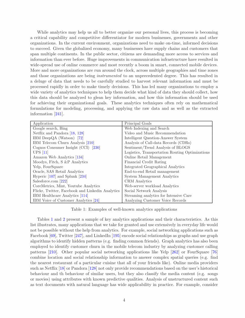
Application Principal GoalsGoogle search, Bing Web Indexing and SearchNetflix and Pandora [18, 128] Video and Music RecommendationIBM DeepQA (Watson) [72] Intelligent Question-Answer SystemIBM Telecom Churn Analysis [210] Analysis of Call-data Records (CDRs)Cognos Consumer Insight (CCI) [230] Sentiment/Trend Analysis of BLOGSUPS [11] Logistics, Transportation Routing OptimizationsAmazon Web Analytics [134] Online Retail ManagementMoodys, Fitch, S &P Analytics Financial Credit RatingYelp, FourSquare Integrated Geographical AnalyticsOracle, SAS Retail Analytics End-to-end Retail managementHyperic [107] and Splunk [234] System Management AnalyticsSalesforce.com [222] CRM AnalyticsCoreMetrics, Mint, Youtube Analytics Web-server workload AnalyticsFlickr, Twitter, Facebook and Linkedin Analytics Social Network AnalysisIBM Healthcare Analytics [114] Streaming analytics for Intensive CareIBM Voice of Customer Analytics [24] Analyzing Customer Voice Records

Table 1: Examples of well-known analytics applications

Tables 1 and 2 present a sample of key analytics applications and their characteristics. As thislist illustrates, many applications that we take for granted and use extensively in everyday life wouldnot be possible without the help from analytics. For example, social networking applications such asFacebook [69], Twitter [247], and LinkedIn [195] encode social relationships as graphs and use graphalgorithms to identify hidden patterns (e.g. finding common friends). Graph analytics has also beenemployed to identify customer churn in the mobile telecom industry by analyzing customer callingpatterns [210]. Other popular social networking applications like Yelp [262] or FourSquare [76]combine location and social relationship information to answer complex spatial queries (e.g. findthe nearest restaurant of a particular cuisine that all of your friends like). Online media providerssuch as Netflix [18] or Pandora [128] not only provide recommendations based on the user’s historicalbehaviour and th behaviour of similar users, but they also classify the media content (e.g. songsor movies) using attributes with known predictive qualities. Analysis of unstructured content suchas text documents with natural language has wide applicability in practice. For example, consider

4

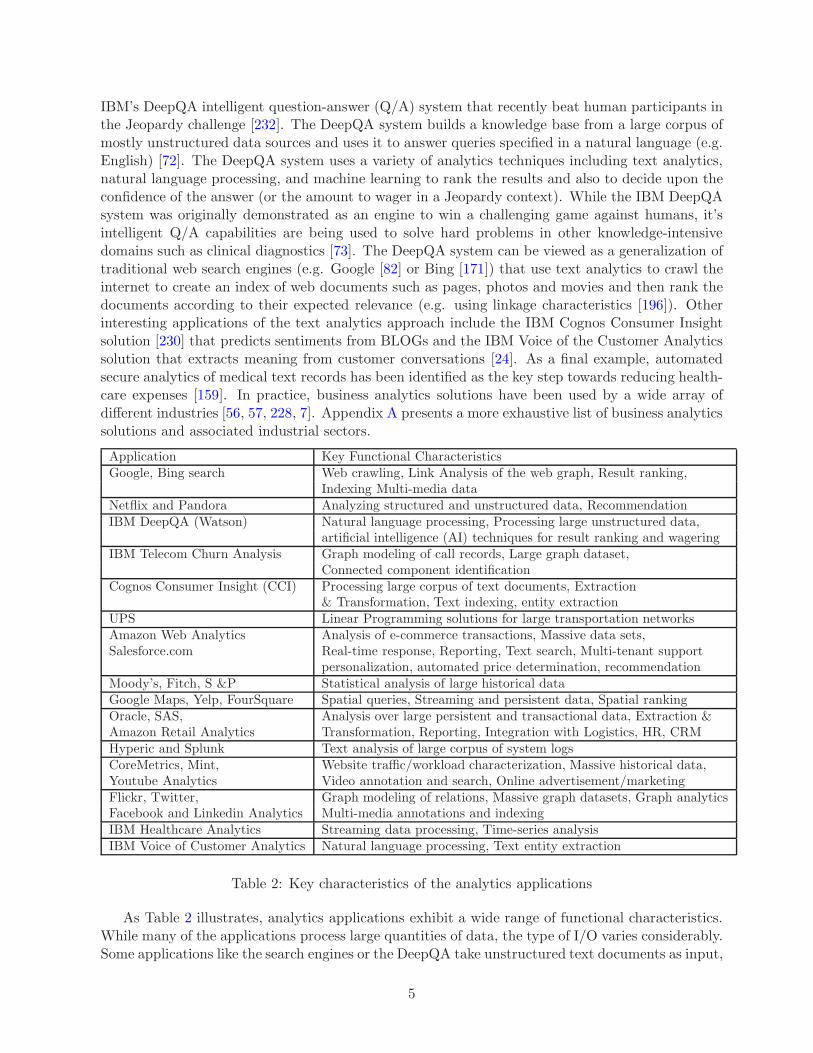
IBM’s DeepQA intelligent question-answer (Q/A) system that recently beat human participants inthe Jeopardy challenge [232]. The DeepQA system builds a knowledge base from a large corpus ofmostly unstructured data sources and uses it to answer queries specified in a natural language (e.g.English) [72]. The DeepQA system uses a variety of analytics techniques including text analytics,natural language processing, and machine learning to rank the results and also to decide upon theconfidence of the answer (or the amount to wager in a Jeopardy context). While the IBM DeepQAsystem was originally demonstrated as an engine to win a challenging game against humans, it’sintelligent Q/A capabilities are being used to solve hard problems in other knowledge-intensivedomains such as clinical diagnostics [73]. The DeepQA system can be viewed as a generalization oftraditional web search engines (e.g. Google [82] or Bing [171]) that use text analytics to crawl theinternet to create an index of web documents such as pages, photos and movies and then rank thedocuments according to their expected relevance (e.g. using linkage characteristics [196]). Otherinteresting applications of the text analytics approach include the IBM Cognos Consumer Insightsolution [230] that predicts sentiments from BLOGs and the IBM Voice of the Customer Analyticssolution that extracts meaning from customer conversations [24]. As a final example, automatedsecure analytics of medical text records has been identified as the key step towards reducing health-care expenses [159]. In practice, business analytics solutions have been used by a wide array ofdifferent industries [56, 57, 228, 7]. Appendix A presents a more exhaustive list of business analyticssolutions and associated industrial sectors.

Application Key Functional CharacteristicsGoogle, Bing search Web crawling, Link Analysis of the web graph, Result ranking,

Indexing Multi-media dataNetflix and Pandora Analyzing structured and unstructured data, RecommendationIBM DeepQA (Watson) Natural language processing, Processing large unstructured data,

artificial intelligence (AI) techniques for result ranking and wageringIBM Telecom Churn Analysis Graph modeling of call records, Large graph dataset,

Connected component identificationCognos Consumer Insight (CCI) Processing large corpus of text documents, Extraction

& Transformation, Text indexing, entity extractionUPS Linear Programming solutions for large transportation networksAmazon Web Analytics Analysis of e-commerce transactions, Massive data sets,Salesforce.com Real-time response, Reporting, Text search, Multi-tenant support

personalization, automated price determination, recommendationMoody’s, Fitch, S &P Statistical analysis of large historical dataGoogle Maps, Yelp, FourSquare Spatial queries, Streaming and persistent data, Spatial rankingOracle, SAS, Analysis over large persistent and transactional data, Extraction &Amazon Retail Analytics Transformation, Reporting, Integration with Logistics, HR, CRMHyperic and Splunk Text analysis of large corpus of system logsCoreMetrics, Mint, Website traffic/workload characterization, Massive historical data,Youtube Analytics Video annotation and search, Online advertisement/marketingFlickr, Twitter, Graph modeling of relations, Massive graph datasets, Graph analyticsFacebook and Linkedin Analytics Multi-media annotations and indexingIBM Healthcare Analytics Streaming data processing, Time-series analysisIBM Voice of Customer Analytics Natural language processing, Text entity extraction

Table 2: Key characteristics of the analytics applications

As Table 2 illustrates, analytics applications exhibit a wide range of functional characteristics.While many of the applications process large quantities of data, the type of I/O varies considerably.Some applications like the search engines or the DeepQA take unstructured text documents as input,

5

while others like the Oracle retail analysis [194] use structured data stored in relational databases.Applications like Google Maps [82], Yelp, or Netflix use both structured and unstructured data.Certain applications such as the search engines process read-only historical data whereas otherapplication such as retail analytics process both historical and transactional data. Still otherapplications, such as some in the health-care domain, work exclusively on streaming data. Inaddition, the data structures used by the analytical applications vary considerably, according tothe scale of data and expected access patterns. These data structures include graphs, relationaltables, lists, numerical matrices, hash-based structures, and binary objects. Finally, analyticsapplications use different classes of algorithms; they vary from statistical quantitative techniques,numerical linear algebraic methods to relational operators and string algorithms.

The main focus of our work is to understand how to effectively optimize analytics applicationson today’s computing systems. This is important both because of the demanding requirements ofanalytics and because systems architecture is currently undergoing a set of disruptive changes. Overthe years, main memory sizes have increased significantly - machines with 1 TB main memory arenot uncommon. The advent of technologies like the phase-change memories (PCMs) could furtherincrease main memory capacities. Thus the applications that were considered out-of-core just afew years ago, can now be executed completely in-memory. Wider usage of streaming applicationshas further increased the importance of in-memory processing. At the same time, prices of harddisk drives (HDDs) are falling precipitously; one can get 1 TB HDD for less than $100. Thus,one can easily build a multi-TB storage system using commodity HDDs. The prices of solid-statedrives (SSDs) are also falling steadily. The SSDs are being increasing used in three-tier systemseither as caches for hot read-only data from HDDs or as faster swap or memory-mapped space formain memories. Availability of cheaper and larger storage systems has made applications with verylarge I/O requirements practical, even into the petabyte range. Thus on the storage side, a cleartrend is emerging in which main memory processing would become increasingly prevalent, mainly forstreaming and large (terabyte size) datasets, and disk-based out-of-core computations would be usedfor petabyte and eventually exabyte scale processing. On the processing side, multi-core processorshave become the norm driving up system parallelism on a curve similar to past increases in singlecore performance. While the commodity desktop processors have been continuously improvingtheir performance and functionality, specialized accelerators such as GPUs and FPGAs are alsobecoming increasingly popular in compute-intensive domains. Hybrid systems that use both theCPUs and GPUs are becoming common-place, both in desktop and mobile domains. Even withthese large improvements in single system performance, applications processing huge data sets arealso exploiting distributed processing to satisfy their appetite for large computing and storageresources. Given the diverse characteristics exhibited by the analytics applications, it is difficultto fine-tune system parameters, both in hardware and software, that can match requirements ofdifferent applications. This problem is further exacerbated as most analytics applications consistof more than one components, each with its unique set of features.

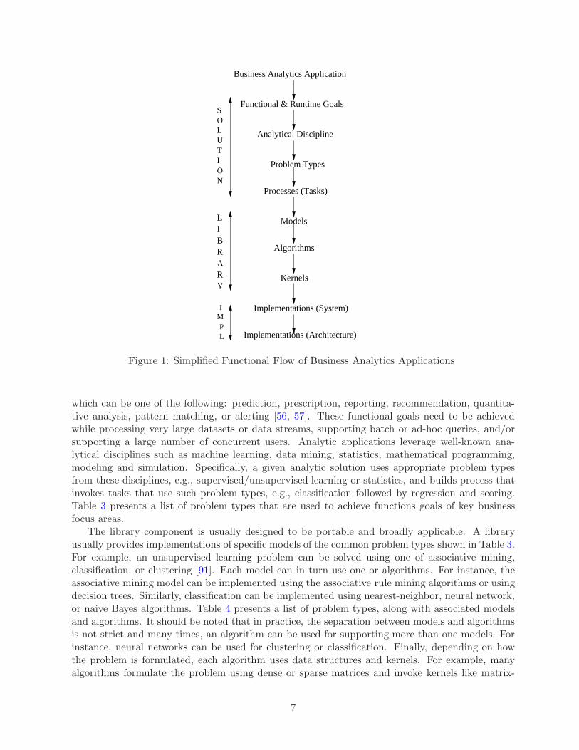
Given the diverse and demanding requirements of analytics and the new technology availablein systems, it is imperative to perform an in-depth study of various analytics applications. Anyinsights would help us identify: (1) optimization opportunities for analytics applications on existingsystems, and (2) features for future systems that match the requirements of analytics applications.Towards achieving these goals, as the first step, we plan to examine the functional flow of analyticsapplications from the usage to the implementation stages. Figure 1 presents a simplified functionalflow of the analytics applications.

As Figure 1 illustrates, execution of an analytics application can be partitioned into three maincomponents: (1) solution, (2) library, and (3) implementation. The solution component is end-user focused and uses the library and implementation components to satisfy user’s functional goal,

6

Y

I

PL

M

Functional & Runtime Goals

Analytical Discipline

Problem Types

Processes (Tasks)

Models

Algorithms

Kernels

Implementations (System)

Implementations (Architecture)

SOLUTION

LIBRAR

Business Analytics Application

Figure 1: Simplified Functional Flow of Business Analytics Applications

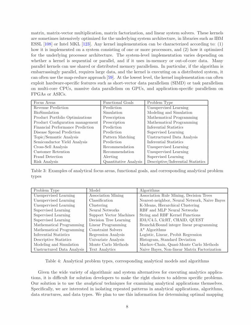
which can be one of the following: prediction, prescription, reporting, recommendation, quantita-tive analysis, pattern matching, or alerting [56, 57]. These functional goals need to be achievedwhile processing very large datasets or data streams, supporting batch or ad-hoc queries, and/orsupporting a large number of concurrent users. Analytic applications leverage well-known ana-lytical disciplines such as machine learning, data mining, statistics, mathematical programming,modeling and simulation. Specifically, a given analytic solution uses appropriate problem typesfrom these disciplines, e.g., supervised/unsupervised learning or statistics, and builds process thatinvokes tasks that use such problem types, e.g., classification followed by regression and scoring.Table 3 presents a list of problem types that are used to achieve functions goals of key businessfocus areas.

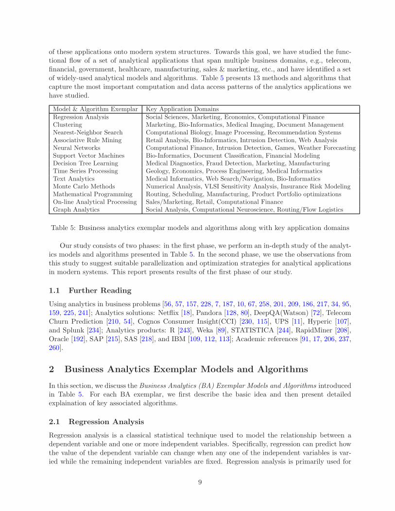
The library component is usually designed to be portable and broadly applicable. A libraryusually provides implementations of specific models of the common problem types shown in Table 3.For example, an unsupervised learning problem can be solved using one of associative mining,classification, or clustering [91]. Each model can in turn use one or algorithms. For instance, theassociative mining model can be implemented using the associative rule mining algorithms or usingdecision trees. Similarly, classification can be implemented using nearest-neighbor, neural network,or naive Bayes algorithms. Table 4 presents a list of problem types, along with associated modelsand algorithms. It should be noted that in practice, the separation between models and algorithmsis not strict and many times, an algorithm can be used for supporting more than one models. Forinstance, neural networks can be used for clustering or classification. Finally, depending on howthe problem is formulated, each algorithm uses data structures and kernels. For example, manyalgorithms formulate the problem using dense or sparse matrices and invoke kernels like matrix-

7

matrix, matrix-vector multiplication, matrix factorization, and linear system solvers. These kernelsare sometimes intensively optimized for the underlying system architecture, in libraries such as IBMESSL [108] or Intel MKL [123]. Any kernel implementation can be characterized according to: (1)how it is implemented on a system consisting of one or more processors, and (2) how it optimizedfor the underlying processor architecture. The system-level implementation varies depending onwhether a kernel is sequential or parallel, and if it uses in-memory or out-of-core data. Manyparallel kernels can use shared or distributed memory parallelism. In particular, if the algorithm isembarrassingly parallel, requires large data, and the kernel is executing on a distributed system, itcan often use the map-reduce approach [59]. At the lowest level, the kernel implementation can oftenexploit hardware-specific features such as short-vector data parallelism (SIMD) or task parallelismon multi-core CPUs, massive data parallelism on GPUs, and application-specific parallelism onFPGAs or ASICs.

Focus Areas Functional Goals Problem TypeRevenue Prediction Prediction Unsupervised LearningBioSimulation Simulation Modeling and SimulationProduct Portfolio Optimizations Prescription Mathematical ProgrammingProduct Configuration management Prescription Mathematical ProgrammingFinancial Performance Prediction Prediction Inferential StatisticsDisease Spread Prediction Prediction Supervised LearningTopic/Semantic Analysis Pattern Matching Unstructured Data AnalysisSemiconductor Yield Analysis Prediction Inferential StatisticsCross-Sell Analysis Recommendation Unsupervised LearningCustomer Retention Recommendation Unsupervised LearningFraud Detection Alerting Supervised LearningRisk Analysis Quantitative Analysis Descriptive/Inferential Statistics

Table 3: Examples of analytical focus areas, functional goals, and corresponding analytical problemtypes

Problem Type Model AlgorithmsUnsupervised Learning Association Mining Association Rule Mining, Decision TreesUnsupervised Learning Classification Nearest-neighbor, Neural Network, Naive BayesUnsupervised Learning Clustering K-Means, Hierarchical ClusteringSupervised Learning Neural Networks RBF and MLP Neural NetworksSupervised Learning Support Vector Machines String and RBF Kernel FunctionsSupervised Learning Decision Tree Learning ID3/C4.5, C&RT, CHAID, QUESTMathematical Programming Linear Programming Branch&Bound integer linear programmingMathematical Programming Constraint Solvers A* AlgorithmsInferential Statistics Regression Analysis Logistic, Linear, Probit RegressionDescriptive Statistics Univariate Analysis Histogram, Standard DeviationModeling and Simulation Monte Carlo Methods Markov-Chain, Quasi-Monte Carlo MethodsUnstructured Data Analysis Text Analytics Naive Bayes, Non-linear Matrix Factorization

Table 4: Analytical problem types, corresponding analytical models and algorithms

Given the wide variety of algorithmic and system alternatives for executing analytics applica-tions, it is difficult for solution developers to make the right choices to address specific problems.Our solution is to use the analytical techniques for examining analytical applications themselves.Specifically, we are interested in isolating repeated patterns in analytical applications, algorithms,data structures, and data types. We plan to use this information for determining optimal mapping

8

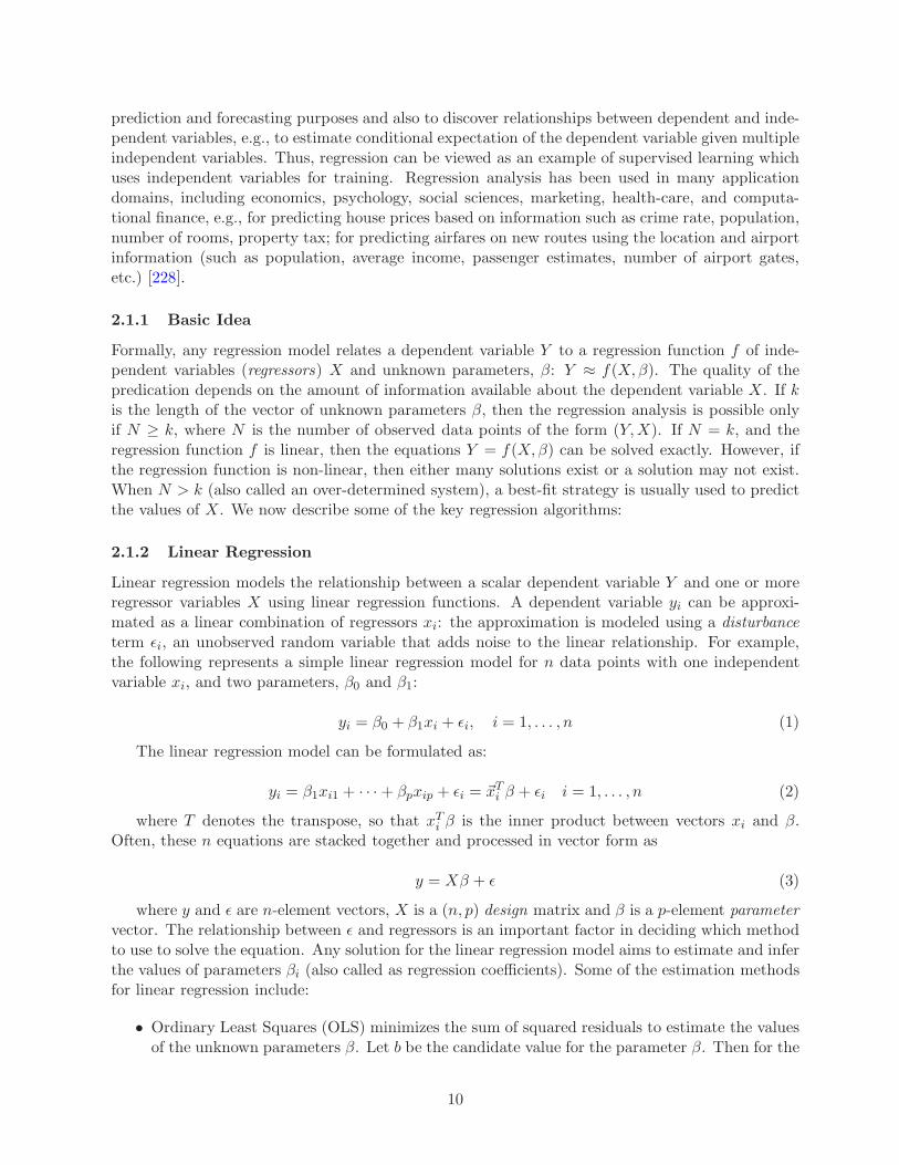
of these applications onto modern system structures. Towards this goal, we have studied the func-tional flow of a set of analytical applications that span multiple business domains, e.g., telecom,financial, government, healthcare, manufacturing, sales & marketing, etc., and have identified a setof widely-used analytical models and algorithms. Table 5 presents 13 methods and algorithms thatcapture the most important computation and data access patterns of the analytics applications wehave studied.

Model & Algorithm Exemplar Key Application DomainsRegression Analysis Social Sciences, Marketing, Economics, Computational FinanceClustering Marketing, Bio-Informatics, Medical Imaging, Document ManagementNearest-Neighbor Search Computational Biology, Image Processing, Recommendation SystemsAssociative Rule Mining Retail Analysis, Bio-Informatics, Intrusion Detection, Web AnalysisNeural Networks Computational Finance, Intrusion Detection, Games, Weather ForecastingSupport Vector Machines Bio-Informatics, Document Classification, Financial ModelingDecision Tree Learning Medical Diagnostics, Fraud Detection, Marketing, ManufacturingTime Series Processing Geology, Economics, Process Engineering, Medical InformaticsText Analytics Medical Informatics, Web Search/Navigation, Bio-InformaticsMonte Carlo Methods Numerical Analysis, VLSI Sensitivity Analysis, Insurance Risk ModelingMathematical Programming Routing, Scheduling, Manufacturing, Product Portfolio optimizationsOn-line Analytical Processing Sales/Marketing, Retail, Computational FinanceGraph Analytics Social Analysis, Computational Neuroscience, Routing/Flow Logistics

Table 5: Business analytics exemplar models and algorithms along with key application domains

Our study consists of two phases: in the first phase, we perform an in-depth study of the analyt-ics models and algorithms presented in Table 5. In the second phase, we use the observations fromthis study to suggest suitable parallelization and optimization strategies for analytical applicationsin modern systems. This report presents results of the first phase of our study.

1.1 Further Reading

Using analytics in business problems [56, 57, 157, 228, 7, 187, 10, 67, 258, 201, 209, 186, 217, 34, 95,159, 225, 241]; Analytics solutions: Netflix [18], Pandora [128, 80], DeepQA(Watson) [72], TelecomChurn Prediction [210, 54], Cognos Consumer Insight(CCI) [230, 115], UPS [11], Hyperic [107],and Splunk [234]; Analytics products: R [243], Weka [89], STATISTICA [244], RapidMiner [208],Oracle [192], SAP [215], SAS [218], and IBM [109, 112, 113]; Academic references [91, 17, 206, 237,260].

2 Business Analytics Exemplar Models and Algorithms

In this section, we discuss the Business Analytics (BA) Exemplar Models and Algorithms introducedin Table 5. For each BA exemplar, we first describe the basic idea and then present detailedexplaination of key associated algorithms.

2.1 Regression Analysis

Regression analysis is a classical statistical technique used to model the relationship between adependent variable and one or more independent variables. Specifically, regression can predict howthe value of the dependent variable can change when any one of the independent variables is var-ied while the remaining independent variables are fixed. Regression analysis is primarily used for

9

prediction and forecasting purposes and also to discover relationships between dependent and inde-pendent variables, e.g., to estimate conditional expectation of the dependent variable given multipleindependent variables. Thus, regression can be viewed as an example of supervised learning whichuses independent variables for training. Regression analysis has been used in many applicationdomains, including economics, psychology, social sciences, marketing, health-care, and computa-tional finance, e.g., for predicting house prices based on information such as crime rate, population,number of rooms, property tax; for predicting airfares on new routes using the location and airportinformation (such as population, average income, passenger estimates, number of airport gates,etc.) [228].

2.1.1 Basic Idea

Formally, any regression model relates a dependent variable Y to a regression function f of inde-pendent variables (regressors) X and unknown parameters, β: Y ≈ f(X,β). The quality of thepredication depends on the amount of information available about the dependent variable X. If kis the length of the vector of unknown parameters β, then the regression analysis is possible onlyif N ≥ k, where N is the number of observed data points of the form (Y,X). If N = k, and theregression function f is linear, then the equations Y = f(X,β) can be solved exactly. However, ifthe regression function is non-linear, then either many solutions exist or a solution may not exist.When N > k (also called an over-determined system), a best-fit strategy is usually used to predictthe values of X. We now describe some of the key regression algorithms:

2.1.2 Linear Regression

Linear regression models the relationship between a scalar dependent variable Y and one or moreregressor variables X using linear regression functions. A dependent variable yi can be approxi-mated as a linear combination of regressors xi: the approximation is modeled using a disturbanceterm ǫi, an unobserved random variable that adds noise to the linear relationship. For example,the following represents a simple linear regression model for n data points with one independentvariable xi, and two parameters, β0 and β1:

yi = β0 + β1xi + ǫi, i = 1, . . . , n (1)

The linear regression model can be formulated as:

yi = β1xi1 + · · ·+ βpxip + ǫi = ~xTi β + ǫi i = 1, . . . , n (2)

where T denotes the transpose, so that xTi β is the inner product between vectors xi and β.Often, these n equations are stacked together and processed in vector form as

y = Xβ + ǫ (3)

where y and ǫ are n-element vectors, X is a (n, p) design matrix and β is a p-element parametervector. The relationship between ǫ and regressors is an important factor in deciding which methodto use to solve the equation. Any solution for the linear regression model aims to estimate and inferthe values of parameters βi (also called as regression coefficients). Some of the estimation methodsfor linear regression include:

• Ordinary Least Squares (OLS) minimizes the sum of squared residuals to estimate the valuesof the unknown parameters β. Let b be the candidate value for the parameter β. Then for the

10

ith data point, the residual is given by yi − xTi b. The sum of squared residuals is a measureof the estimation quality:

S(b) =

n∑

i=1

(yi − xTi b)2 = (y −Xb)T (y −Xb) (4)

The value of b that minimizes this sum is called the OLS estimator for β and its solution canbe found by an explicit formula:

β = (1

n

n∑

i=1

xixTi )

−1.1

n

n∑

i=1

xiyi = (XTX)−1XT y (5)

After estimating the values of β, the predicated values from the regression will be

y = Xβ (6)

• Generalized Least Squares (GLS) estimation is used when the variances in observations areunequal or when there is a certain degree of correlation between the observations. Thismodel assumes that the conditional mean of Y given X is a linear function of X, whereas theconditional variance of Y given X is a known matrix Ω, i.e.,

E[ǫ|X]0, V ar[ǫ|X] = Ω (7)

The Generalized least squares method estimates β by minimizing the squared Mahanobislength of the residual vector:

S(b) = (y −Xb)TΩ−1(y −Xb) (8)

Like the OLS estimator, this objective has a quadratic form and can be solved using anexplicit formula:

β = (XTΩ−1X)−1XTΩ−1y (9)

2.1.3 Non-linear Regression

The non-linear regression model is characterized by the fact that the dependent variables Y are re-lated to the regressor variables X via a non-linear relationship on one or more unknown parameters,β. A non-linear regression model has the following form:

yi = f(xi, β) + ǫi, i = 1, . . . , n (10)

where the function f(xi, β) is nonlinear as it cannot be expressed as a linear combination ofthe parameters, β and ǫi are random errors. One of the most common nonlinear function is theexponential decay or growth model [231]: f(x, β) = β1exp(−β2x). Other nonlinear functionsinclude logarithmic, trigonometric, power, and Gaussian functions.

Unlike linear regression, there is no closed-form expression for finding best-fitting parameters.The regression parameters β can be estimated by minimizing a suitable goodness-of-fit expressionwith respect to β. One popular approach is to minimize the sum of squared residuals

11

n∑

i=1

[yi − f(xi, β)]2 (11)

using the nonlinear least squares method that uses the Gauss-Newton numerical method. Insome cases, maximum likelihood or weighted least squares estimation is used.

Alternatively, in some cases, the nonlinear function can be transformed to a linear model. Thetransformed model can then be estimated using linear regression approaches. For example, anexponential regression function, Y = aeβX , can be transformed using a logarithm on both sides asln(Y ) = ln(a) + βX. The parameters β can then be estimated using a linear regression of ln(Y )on X.

2.1.4 Logistic Regression

The logistic regression is used for prediction of the probability of occurrences of an event (e.g., deathby heart attack) by fitting data to a logistic function, f(z) = 1

1+e−z . The variable z is a measureof the total contributions of all the independent variables while f(z) represents probability of aparticular outcome, given the set of independent variables. The variable z is usually defined as

z = β0 + β1x1 + · · · + βkxk (12)

and for any value of z, the output f(z) varies between 0 and 1.Logistic regression analyzes binomially distributed data of the form Yi ∼ B(ni, pi), for i =

1, . . . , n, where the number of Bernoulli trials ni are known, and the probabilities of success pi areunknown. This model proposes for each observation i, there is a set of k explanatory variables thatcan be viewed as being in a k-dimensional vector Xi. The model can then be represented using

pi = E(Yi

ni|Xi) (13)

The logistic function of pI can be computed as its inverse-logit function defined as

logit−1(pi) =1

1+exp(−pi)= exp(pi)

1+exp(pi)(14)

where pi can modeled as a linear function of the Xi.

β0 + β1x1,i + · · ·+ βkxk,i (15)

The parameters βi can then be estimated by maximum likelihood approach via the iterativelyre-weighted least squares method that can use the Gauss-Newton numerical algorithm.

2.1.5 Probit Regression

Probit regression is used for predicting binary outcomes of an event. Let the regression variable Ybe a binary variable (i.e., it can have only two possible outcomes) and X be the set of regressorvariables that have influence on the outcome of Y. Then the probit model can be specified as:

Pr(Y = 1|X) = Φ(XTβ) (16)

where Pr denotes probability, and Φ denotes the Cumulative Distribution Function (CDF) ofthe normal distribution. The regression coefficients β can then be estimated using the Fisher’smaximum likelihood method on the joint log-likelihood metric of the input data set yi, xi

ni=1.

12

2.1.6 Further Reading

Algorithms [91, 260]; Packages: R [243], Weka [89], IBM SPSS [119], RapidMiner [208], STATIS-TICA [244], Oracle Data Miner [193], and SAS [218]; Applications [228, 237, 231].

2.2 Clustering

Clustering is a process of grouping together entities from an ensemble into classes of entities thatare similar in some sense. Clustering is also called data segmentation [91, 228] as it partitions largedatasets into segments of similar and dissimilar datasets. Clustering is an example of unsupervisedmachine learning and is being used in a wide variety of applications e.g., in market segmentationfor partitioning the customers according to gender, interests, etc., in gene sequence analysis toidentify gene families, in medical imaging for differentiating key features in PET scan images, andin clustering documents based on semantic information [258].

2.2.1 Basic Idea

Any clustering algorithm needs to effectively identify and exploit relevant similarities in underlyingpotentially disparate data sources. The similarity can be expressed using either geometric distance-based metric (e.g., using either Euclidean or Minkowski metric) or conceptual relationships in thedata. The input data can be noisy, of different types (interval-based, binary, categorical, ordinal,vector, and mixed etc.), have high dimensions, and have large size (e.g., millions of objects). Thusthe key challenges before any clustering algorithm are the effective use of the similarity metric,exploitation of intrinsic characteristics of the data, support for large number of dimensions, largedata sets, and different cluster shapes.

Current approaches to solving the clustering problem can be broadly classified into parametricand non-parametric approaches. The parametric or model-based methods assume that the inputdata is associated with a certain probability distribution and the clustering to designed to fit thedata to some mathematical model [91]. The non-parametric methods exploit spatial properties(e.g., distance or density) of the input data. Clustering algorithms also differ depending on thedimensionality of the datasets [140]. We now discuss some of the key clustering algorithms.

2.2.2 K-Means Clustering

The k-means clustering algorithm [156, 97] is an example of a partitioning method that constructsk partitions from a database of n objects, where each partition represents a cluster and k ≤ n. Eachcluster contains at least one object and an object lies in only one cluster. A partitioning algorithmcreates an initial assignment of objects to partitions and then iterative relocation technique areused [91] to move objects among the groups. The objects in a group are considered to be closer toeach than objects in different clusters. In the k-means algorithm, the cluster similarity is measuredas the mean value of objects, which can be viewed as the cluster’s centroid or center of gravity.

The k-means algorithms works as follows: Given the number of partitions k, it first randomlyselects k objects, each of which initially represents a cluster mean. For the remaining objects,every object is then assigned to one of the k clusters, to which it is the most similar, based onthe distance of the object and the cluster mean. Once, the object is assigned to a cluster, a newmean is computed. Using the new cluster mean value, the objects are re-distributed to the clustersbased on which new cluster center is the nearest.The iterative relocation process continues until aconvergence criterion is met. The k-means algorithm uses the following square-error criterion forconvergence:

13

E =

k∑

i=1

∑

p∈Ci

|p−mi|2 (17)

where E is the sum of the square error for all objects in the data set, p is the point representinga object and mi is the mean of a cluster Ci. This criterion tries to make the k clusters to be ascompact and separate as possible. The algorithm runs in O(nkt) time, where n is the number ofobjects, k is the number of clusters, and t is the number of iterations, k ≪ n and p≪ n.

The k-means algorithms works only on data whose mean can be computed (e.g., it is not possibleto compute a mean value for categorical datasets). The algorithm also requires the number ofclusters k to be defined a priori. The algorithm can not discover clusters with different shapesand is sensitive to noise and outliners as they can significantly affect calculations of the meanvalue. One variation of the k-means problem, the k-modes method uses modes as a measure ofsimilarity for categorical objects and a frequency-based update method [38]. Another variation,the k-medoid, reduces the effect of noise and outliners using the following absolute-error criterionfor convergence [91].

E =k

∑

i=1

∑

p∈Ci

|p− oi| (18)

where E is the absolute error for all objects in the data set, p is the point representing a objectand oi is the representative object (a medoid) of a cluster Ci. Initially, the medoids are chosenrandomally and they are iteratively refined as the algorithm progresses.

2.2.3 Hierarchical Clustering

Hierarchical clustering methods group data objects into a tree of clusters. Hierarchical clusteringoften produces data clusters that can be viewed graphically using a dendrogram. Hierarchicalmethods can be classified into: (1) agglomerative, i.e., those use a bottom-up strategy to constructincreasing large clusters until certain termination conditions are met, and (2) divisive, i.e., thosethat start from a single cluster and subdivide it into smaller pieces until termination conditions aremet.

The most popular hierarchical clustering algorithm, BIRCH [265], uses the agglomerative strat-egy. BIRCH uses a two-step strategy to improve I/O scalability and clustering flexibility. In thefirst micro-clustering stage, it uses the hierarchical clustering strategy to build an initial set of in-memory clusters, that summarize the information in the original data. The second macro-clusteringphase processes these summarized in-memory clusters (i.e., it does not fetch the raw data again)using any clustering method, e.g., iterative partitioning, and computes the final clustering.

The BIRCH algorithm uses two concepts of clustering features and clustering tree to summarizethe input data. A clustering feature is a three-dimensional vector summarizing statistics for thegiven cluster: the zeroth, first, and second moments of the cluster. For a cluster ci with n d-dimensional points, the cluster feature CFi is defined as CFi =< n,LS, SS >, where n is thenumber of points in the cluster ci, LS is the linear sum of the n points (i.e.,

∑ni=1 xi), and SS

is the square sum of the data points (i.e.,∑n

i=1 xi2). The clustering features are additive; thus a

clustering feature for a newly merged cluster can be computed by simply adding clustering featuresof the two original clusters. The clustering features provide sufficient information for the BIRCHalgorithm to make the clustering decisions.

The clustering tree is a height-balanced tree that stores clustering features for the hierarchicalclustering. Each node of the clustering tree represents a set of clusters. The maximum number of

14

children per non-leaf nodes of a CF tree is bound by a branching factor, B. The size of the leafnodes is determined by the threshold, T representing the maximum diameter of the clusters storedin the leaf nodes, where diameter (the average pairwise distance within a cluster) of a cluster ciwith n elements is computed as:

D =

√

∑ni=1

∑nj=1 (xi − xj)

2

n(n− 1)(19)

The branching factor and threshold, along with the data page size P , determine size of theCF tree leaf nodes, L, and in turn, the CF tree size. To optimize the I/O costs, the BIRCHalgorithm performs clustering in two phases: in the first phase, a CF tree is created using a singlescan of the underlying data (optionally, additional passes are used to improve the representationquality by reducing the impact of outliners). The size of the CF tree is determined by choosing theappropriate values of the branching factor, threshold, and data page size. The CF tree is then builtby incrementally inserting data into a sub-tree rooted at a root node. For every data point, theCF tree is recursively traversed; an appropriate leaf node is identified using a inter-cluster distancefunction using the Euclidean, Manhattan, or log-likelyhood centroid values [265, 41]. Once the leafis found, the data point can be absorbed into the leaf (i.e., into its CF vector) if it doesn’t violatethe threshold value. Otherwise a new leaf entry (a CF vector) is created. Once the leaf size exceedsL, a new leaf node is created by splitting. At the end of the first phase, the CF tree representssummarized version of the input data using the CF vectors.

In the second phase, BIRCH applies a standard clustering algorithm (e.g., iterative clustering)on the CF tree leaves to determine the final clustering of the input data. The computationalcomplexity of the BIRCH algorithm is O(n) and in most cases, the algorithm requires only one I/Opass.

2.2.4 EM Clustering

The Expectation-Maximization (EM) clustering is a model-based approach that extends the k-means partitioning algorithm. The EM clustering algorithm assumes that the underlying data isa mixture of the k probability distributions (referred to as component distributions), where eachdistribution represents a cluster. The key problem for any model-based algorithm is to estimatethe parameters of the probability distributions so as to best fit the data.

The EM algorithm [62, 91] is an iterative refinement algorithm that extends the k-mean paradigm:it assigns a data item to a cluster according to a weight representing the probability of membership(unlike the cluster mean metric used in the k-means algorithm). The new means of these clustersare then computed using the weighted measures.

The most common version of the EM algorithm learns a mixture of Gaussian distribution [25]. Itstarts with an initial estimate of the parameters of the mixture model, referred to as the parametervector. Each data item is assigned a probability that it would possess a certain set of attributesgiven that it was a member of a given cluster. The items are then re-scored against the mixturedensity produced by the parameter vector and then the items are used to update the parameterestimates. The complexity of the EM algorithm is linear in d (the dimensions or features of theinput data), n (the number of data items), and t (the number of iterations) (O(dnt)).

The EM algorithm can be described as follows:

1. (Initialization): Make an initial guess of the parameter vectors by randomly selecting k itemsto represent cluster centers and making guesses for probability distribution parameters, i.e.,mean, mk, and expectation, Ek.

15

2. (Expectation and Maximization) This step iteratively refines the parameter guesses using thefollowing two steps:

(a) Expectation: Assign each item xi to Cluster Ck with the probability

P (xi ∈ Ck) = p(Ck|xi) =p(Ck)p(xi|Ck)

p(xi)(20)

This step calculates the probability of cluster membership of object xi, for each of theclusters. These probabilities are the expected cluster memberships of object xi.

(b) Maximization: Use the probability calculated from above to refine the model parameters.For example:

mk =1

n

n∑

i=1

xiP (xi ∈ Ck)∑

j P (xi ∈ Cj)(21)

This step maximizes the likelihood of the distributions given the data.

2.2.5 Further Reading

Algorithms: K-means [156, 97, 38], Hierarchical Clustering [265, 41], EM [62], PROCLUS [2] andCLIQUE [3]; Packages: R [243], Weka [89], IBM SPSS and InfoSphere DataMining [118, 112],RapidMiner [208], STATISTICA [244], Oracle Data Miner [193] and SAS [218]; Applications [91,228, 187].

2.3 Nearest Neighbor Search

Nearest neighbor search is an optimization problem for finding the closest points in a metric space.This problem of identifying points from an ensemble of points that are in some defined proximityto a given query point has been applied for classification and clustering purposes in multiple appli-cation domains such as distributed systems, image processing, data mining, computational biology,data compression, and machine learning. The notion of proximity varies from domain to domainand is usually formulated using a suitable metric function (e.g., Euclidean distance for spatial prox-imity). For example, the online media providers such as Netflix and Pandora use nearest neighboralgorithms to suggest movies or songs that match a particular taste of a particular user [128, 18].Nearest neighbor algorithms have also been used for finding similarities in multi-media data (e.g.,videos) to detect any copyright violations [120]. Other well-known applications of the nearestneighbor search algorithm include control systems, robotics, and drug discovery [236, 124, 22].

2.3.1 Basic Idea

Formally the nearest neighbor problem can be defined as follows: Given a set S of n points insome metric space (X, d), the problem is to preprocess S so that given a query point p ∈ X, onecan efficiently find a q ∈ S that minimizes d(p, q). In practice, several variations of this definitionare implemented as per input data characteristics and runtime constraints. Broadly, the existingsequential nearest neighbor solutions can be classified as per the dimensionality of input data, typeof metric used in proximity calculations, result cardinality (e.g., top-k and all-pairs ), and data size(e.g., Terabyte datasets).

The key aspect of any nearest neighbor algorithm is the metric function used for calculatingthe proximity distance between the input data points. The most widely used metric in the nearest

16

neighbor algorithms is the Euclidean distance: distance between any two points pi and pj in a d-

dimensional space can be computed as |~pi− ~pj|=√

∑k=dk=1 (pik − pjk)

2, where pik is the kth component

of the vector ~pi. In practice, the Euclidean distance has proven to be effective for low-dimensionaldata. For high-dimensional data, more generalized forms of metric distances are employed (e.g.,Hamming distance) [248]. In the case of two-dimensional data, the nearest neighbor problem canbe solved by using Voronoi diagrams [189]. For datasets with very high dimensionality (e.g., incomputer vision), these search algorithms provide sub-linear performance. One approach to dealwith this inefficiency is to define an approximate version of the nearest neighbor problem: thisversion of the problem identifies points from an ensemble of points whose distance from the givenquery point is no more than (1 + ǫ) times the distance of the true kth nearest-neighbor.

2.3.2 K-d Trees

The k-d tree algorithm addresses the precise nearest neighbor problem [20, 21, 77]. The k-d tree isa binary tree used for representing k-dimensional data using recursive hyperplane decomposition.Each node of the k-d tree represents a region of the input dataset and its partitioning. Each levelof the k-d tree covers the entire dataset. In k dimensions, a record is represented by k keys, i.e.,each record can be represented by a k element vector of real values, where each element representsa position in the kth dimension. The k-d tree is then constructed by recursively selecting one ofthe k coordinates as the discriminator dimension and then partitioning the dataset into the subsetof vectors according to a certain partition value. For example, the original k-d tree design [20], thediscriminator D at each tree level L is computed as D = L mod k + 1, and a median or randomvalue for the chosen coordinate is selected as the partition value. During the query process, thetree is recursively traversed from the root: at every level, the value of the discriminator coordinateof the query record is compared against the partition value and either the left or right path ischosen for further traversal. When the traversal reaches a leaf node, the query record is comparedwith the records in the leaf, and a list of the m closest records is maintained. In some cases, itmight be required to traverse nearby nodes to validate the current list of nearest neighbors. Thissituation arises in those scenarios when the minimum distance is greater than the radius of thegeometric region represented by the tree node. Overall, for a dataset of N k-dimensional records,the tree search requires O(logN) time, with O(N) space consumption. The k-d tree is very effectivefor small dimensionalities. As the number of dimensions increases, the quality of discriminationdegrades as the proximity calculations are based only on a subset of coordinates.

2.3.3 Approximate Nearest Neighbor (ANN)

The ANN algorithm uses hierarchical space decomposition for solving the approximate nearestneighbor problem for low-dimensional data. The ANN algorithm represent points in a d-dimensionalspace using a balanced box-decomposition (BBD) tree with O(log n) depth [12]. ANN recursivelysub-divides the space into a collection of cells, each of which is either an axis-aligned d-dimensionalfat (i.e., the ratio between the longest and shortest sides is bounded) rectangle or the set-theoreticdifference of two rectangles, each enclosed within the other. Each node of the tree is associatedwith a cell. Thus, it is associated with all points contained within the enclosed cells. Each leaf cellis associated with a single point lying within the bounding rectangle of the cell. The leaves of thetree span the entire space. The ANN tree has O(n) nodes and can be built in O(dn log n) time.During the querying process, for a given query point q, a priority queue of the internal nodes of theBBD-tree is created, where priority of a node is inversely related to the distance between the querypoint and the cell corresponding to the node. The highest priority node is then selected for recursive

17

descent towards the leaves. As the descent progresses, for every cell visited, the distance from qto the point associated with cell is computed and the priority queue is updated appropriately. Letp denote the closest point seen so far; as soon as the distance from q to the current leaf exceedsdist(q,p)(1+ǫ) , the search can be terminated.

2.3.4 Locality Sensitive Hashing (LSH)

The locality-sensitive hashing (LSH) algorithms are designed for solving the approximate nearestneighbor problem for very high-dimensional data sets (e.g., with a million feature vectors). Thekey idea behind the LSH algorithms is to hash points using several hash functions to ensure thatfor each function, the probability of collision is much higher for points that are close to each otherthan for those that are far apart [121, 8]. Then for the query point, one can determine its nearestneighbors by the hashing the query point and retrieving the points in the bucket containing thatpoint. The LSH method relies on a family of hash functions that have the property that if twopoints are close, then they hash to same bucket with high probability; if they are far apart, theyhash to the same bucket with low probability. Formally, a function family H = h : S → U is(r1, r2, p1, p2) − sensitive, where r1 < r2, p1 > p2, for a distance function D if for any two pointsp, q ∈ R

d, the following properties hold

1. if p ∈ B(q, r1), then PrH[h(q) = h(p)] ≥ p1, and

2. if p /∈ B(q, r2), then PrH[h(q) = h(p)] ≤ p2

where B(q, r) denotes a hypersphere of radius r centered at q. For a LSH family H to be useful,it has to satisfy p1 > p2. By defining a family of LSH functions, namely a(r, r(1 + ǫ), p1, p2)-sensitive hash family, the (1+ ǫ) approximate nearest neighbor problem can be solved. [8] describea methodology for selecting a set of appropriate hash functions for LSH. For example, for binaryvectors from 0, 1d, H can be defined as a family of functions which contains all projections of theinput point on one of the coordinates, i.e., H contains all functions hi from 0, 1

d to 0, 1, suchthat hi(p) = pi. Choosing one hash function uniformly at random from H means that h(p) returnsa random coordinate of p [121, 8]. This approach can be used for cases when Hamming distanceis used for defining locality. Another example uses the hash function ha,b(v) : R

d → N to map ad-dimensional vector v onto a set of integers. The hash function ha,b(v) is defined as ⌊a·v+b

r⌋, where

some ~a is a d dimensional vector with entries chosen independently from a stable distribution andb is a real number chosen uniformly from the range [0, r] [55].

2.3.5 Ball and Metric Trees

The Ball [191, 190, 189] and Metric trees [42, 175, 149] are two related hierarchical data structuresdesigned to support nearest neighbor queries on high-dimensional datasets. A Ball tree is a completebinary tree in which each node represents a hyper-sphere in the n-dimensional Euclidean space (aball). Each ball is represented by n + 1 floating point values which specify the coordinates of itscenter and the Euclidian length of its radius. A Ball tree is constructed such that an interior node’sball is the smallest which contains the balls of its children. Only the leaves of the tree hold relevantinformation; the interior nodes are used only to guide efficient search to the leaf nodes. Unlike thek-d trees, sibling regions in Ball trees can intersect and need not partition the entire space. Tofind the nearest neighbor for a given query point, the Ball tree algorithm finds the smallest ballcentered at the query point and containing a point that can be selected as the nearest neighbor.

18

The selection procedure employs recursive branch-and-bound strategy that tries to find increasinglysmaller and tighter balls by pruning searches over internal nodes.

Metric trees are closely related to Ball trees: metric tree use generalized metric distance [248]between points. Each node n of the metric tree contains two fields: npivot and nradius. The metrictree is constructed such that for all nodes x owned by a node n, D(npivot, x) ≤ nradius, where Dis the distance metric. If a node n contains less than some threshold Rmin number of point, it isconsidered as a leaf node, otherwise n is considered as an internal node, and has two child nodes.The child nodes partition the points owned by the node n using the pivot value. There are severalways of choosing the pivot value; most common pivot values include median or centroid. Each nodeof the metric tree also has a hyper-sphere (ball) with the radius nradius. Note that at a node n, thepivot value can cause uneven partition of the dataset, and the corresponding balls can overlap (asin the Ball tree). The pivot partitioning ensures that a metric tree has log(n) depth [149]. Metrictrees can be queried using a recursive branch-and-bound strategies similar to the Ball trees. Atall times, the metric tree search algorithm maintains a candidate nearest neighbor, which is thenearest neighbor to the query point q it finds so far while traversing the tree. Correspondingly, thenearest distance rnn is maintained. At a node n to be traversed, the algorithm checks if there isany point owned n that falls within the distance rnn from the query point q. If not, the subtreerooted at the node n is not traversed.

2.3.6 Spill Trees

Spill trees [150, 151] are a variant of the metric tree; unlike metric trees, the spill tree childrencan share points. A spill tree internal node has two children and its dataset split into over thetwo children nodes using an overlap region. The amount of overlap improves the result quality,but reduces the query search performance. Therefore, in practice, a hybrid version of the spill treeis used, where only datasets of certain nodes are split using the overlap approach. Querying aspill tree uses a combination of branch-and-bound and non-backtracking approaches. The subtreesrooted at overlap nodes are traversed using the non-backtracking approach, while the non-overlapnodes are traversed using traditional branch-and-bound strategies (similar to the metric trees).

2.3.7 Further Reading

Basic idea [248, 189]; Algorithms: KD-Tree [20, 21, 77], ANN [12]; LSH [121, 8, 55], Ball Trees [191,190, 189], Metric Trees [42, 175, 149], Spill Trees [150, 151], and Cover Trees [23]; Packages:ANN [176]; Applications [18, 128, 187, 91, 236, 124, 22].

2.4 Association Rule Mining

Association rule mining is a key data mining method used for discovering relationships betweenvariables. Agrawal at al [4] first proposed using association rule mining for identifying relationshipsbetween items purchased in retail stores, a process widely known as the market-basket analysis(e.g., Amazon’s ”people who bought an item x, also bought items y, z, . . .” feature). An exampleof an association rule is c% of customers that purchased items X and Y, also bought item Z withpercentage d% . Over the years, this method has been applied to more complex data patternssuch as sequences, trees, graphs, etc., and different application domains such as bio-informatics,intrusion detection, and web-usage analysis [4, 5, 258, 260].

19

2.4.1 Basic Idea

Formally, the association rule mining processes a set (or database) D of transactions, where eachtransaction T is a set of items such that T ⊆ I, where I = i1, i2, · · · , im is a set of literals, calleditems. Each transaction is associated with a unique identifier, called TID. By association rule, wemean an implication of the form X =⇒ Ij , where X is a set of some items in I and Ij is a singleitem in I that is not present in X. The rule X =⇒ Y in the transaction set D has a confidencec if c% of transactions in D that contain X also contain Y . The rule X =⇒ Y has support sin the transaction set D if s% of transactions in D contain X ∪ Y [4, 5]. While confidence is ameasure of the rule’s strength, support corresponds to statistical significance. The support of arule X =⇒ Y is defined as supp(X =⇒ Y ) = supp(X ∪ Y ). The confidence of this rule is definedas conf(X =⇒ Y ) = supp(X ∪ Y )/supp(X). Given a set of transactions D, the problem of miningassociation rules is to generate all association rules that have support and confidence greater thanthe user-specified minimum support (called minsup) and minimum confidence (called minconf ).The problem of discovering all association rules can be decomposed into two subproblems [4, 5, 101]:

• Find all sets of items (itemsets) that have transaction support above minsup. The supportfor an itemset is the number of transactions that contain the itemset. Itemsets with at leastminsup are called large (frequent) itemsets, and all others are small itemsets.

• Use the frequent itemsets to discover the desired rules. For every frequent itemset l, we findall non-empty subsets of l. Note that the support attribute follows the downward closureproperty: all subsets of a frequent itemset must be frequent. For every such subset a, weoutput a rule of the form a =⇒ (l − a) if the ratio of support(l) to support(a) is at leastminconf. One needs to consider all subsets of l to generate rules with multiple consequences.The number of rules can grow exponentially with the number of items, but the choices canbe pruned using both minsup and minconf.

Once the associated rules are computed, further pruning may be required to select the mostuseful rules [133].

The key task in the association rule mining process is to find all itemsets that are frequentwith respect to a given minimal threshold minsupp. All existing associative rule mining algorithmsemploy the downward closure property of the itemset support for pruning the search space: everysubset of a new frequent itemset must be frequent. These algorithms can be classified by how thesearch space is traversed to construct itemsets [101]: the breadth-first search (BFS) algorithmscompute all itemsets of size k− 1 before building the itemsets of size k, while the depth-first search(DFS) algorithms, hierarchically compute all possible itemsets of size k from a list of frequentitemsets of size j (j < k), before processing other itemsets of size j.

Frequent and potentially frequent itemsets are called candidate itemsets. There are two com-mon ways of computing support values of these candidate itemsets. The first approach directlycounts occurrences of that itemset in all D transactions. The second approach uses set intersectionto compute the support values of the itemsets. For every item in the transaction set, a list ofidentifiers (TIDs) that correspond to the transactions containing that item is maintained (tidlist).Accordingly, tidlists also exist for every itemset X and denoted by X.tidlist. The tidlist of a can-didate C = X ∪ Y can be obtained as C.tidlist = X.tidlist ∩ Y.tidlist. The actual support of theitemset C can then be computed as |C.tidlist|.

Based on the strategy for traversing the candidate search space (i.e., DFS vs. BFS) and forcomputing the support values (i.e., direct counting vs. intersection), the association rule miningalgorithms can be partitioned into 4 key families [101] (Table 2.4.1).

20

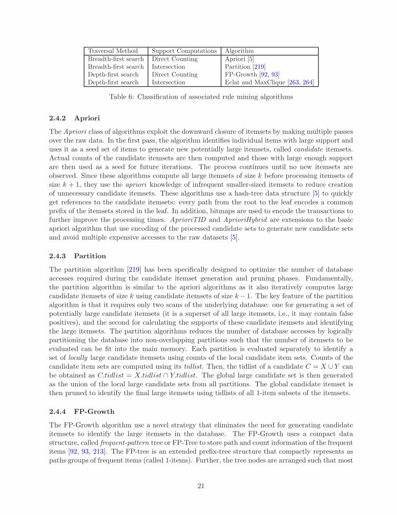
Traversal Method Support Computations AlgorithmBreadth-first search Direct Counting Apriori [5]Breadth-first search Intersection Partition [219]Depth-first search Direct Counting FP-Growth [92, 93]Depth-first search Intersection Eclat and MaxClique [263, 264]

Table 6: Classification of associated rule mining algorithms

2.4.2 Apriori

The Apriori class of algorithms exploit the downward closure of itemsets by making multiple passesover the raw data. In the first pass, the algorithm identifies individual items with large support anduses it as a seed set of items to generate new potentially large itemsets, called candidate itemsets.Actual counts of the candidate itemsets are then computed and those with large enough supportare then used as a seed for future iterations. The process continues until no new itemsets areobserved. Since these algorithms compute all large itemsets of size k before processing itemsets ofsize k + 1, they use the apriori knowledge of infrequent smaller-sized itemsets to reduce creationof unnecessary candidate itemsets. These algorithms use a hash-tree data structure [5] to quicklyget references to the candidate itemsets: every path from the root to the leaf encodes a commonprefix of the itemsets stored in the leaf. In addition, bitmaps are used to encode the transactions tofurther improve the processing times. AprioriTID and AprioriHybrid are extensions to the basicapriori algorithm that use encoding of the processed candidate sets to generate new candidate setsand avoid multiple expensive accesses to the raw datasets [5].

2.4.3 Partition

The partition algorithm [219] has been specifically designed to optimize the number of databaseaccesses required during the candidate itemset generation and pruning phases. Fundamentally,the partition algorithm is similar to the apriori algorithms as it also iteratively computes largecandidate itemsets of size k using candidate itemsets of size k− 1. The key feature of the partitionalgorithm is that it requires only two scans of the underlying database: one for generating a set ofpotentially large candidate itemsets (it is a superset of all large itemsets, i.e., it may contain falsepositives), and the second for calculating the supports of these candidate itemsets and identifyingthe large itemsets. The partition algorithms reduces the number of database accesses by logicallypartitioning the database into non-overlapping partitions such that the number of itemsets to beevaluated can be fit into the main memory. Each partition is evaluated separately to identify aset of locally large candidate itemsets using counts of the local candidate item sets. Counts of thecandidate item sets are computed using its tidlist. Then, the tidlist of a candidate C = X ∪ Y canbe obtained as C.tidlist = X.tidlist ∩ Y.tidlist. The global large candidate set is then generatedas the union of the local large candidate sets from all partitions. The global candidate itemset isthen pruned to identify the final large itemsets using tidlists of all 1-item subsets of the itemsets.

2.4.4 FP-Growth

The FP-Growth algorithm use a novel strategy that eliminates the need for generating candidateitemsets to identify the large itemsets in the database. The FP-Growth uses a compact datastructure, called frequent-pattern tree or FP-Tree to store path and count information of the frequentitems [92, 93, 213]. The FP-tree is an extended prefix-tree structure that compactly represents aspaths groups of frequent items (called 1-items). Further, the tree nodes are arranged such that most

21

frequent items have longest common prefix paths. Thus, the FP-tree performs a DFS traversal ofthe database and generates a compact representation. The item-set mining algorithm then workson the FP-tree, rather than on the raw database. The mining algorithm uses the 1-item nodes asinitial suffixes and builds increasingly larger frequent patterns by concatenating shorter frequentpatterns. The mining algorithm uses least frequent 1-items to build the suffix paths, this improvingthe selectivity of the algorithm. The mining algorithm builds a partial conditional tree using thesuffixes under consideration, and uses it as a guide to build larger frequent patterns. Thus, unlikethe Apriori and partition algorithms, it does not generate level-wise candidate itemsets, but usesknown shorter suffix patterns to build larger frequent patterns,

2.4.5 Eclat and MaxClique

The Eclat and MaxClique family of algorithms [263, 264] aim to reduce the I/O costs of candidategeneration by identifying relevant candidate itemsets using structural relationships among the can-didate itemsets. Specifically, these algorithms view the creation of candidate itemsets using thedownward closure property as a lattice, and use two strategies, one based on equivalence classes,and another on maximal cliques in a hypergraph, to predict the useful candidate itemsets (calledthe potential maximal itemsets). These itemsets logically induce a sub-lattice, which is then tra-versed using either bottom-up or hybrid (top-down and bottom-up) strategy to generate all frequentitemsets. Each sub-lattice is processed in its entirety before progressing to the next sub-lattice.These algorithms assume that the transactions database is represented in the vertical format usingtidlists, and as in the previous case, the itemset frequency can be calculated by intersection. Thesefeatures enable the Eclat and MaxClique to compute the frequent itemsets in a single databasescan.

2.4.6 Further Reading

Basic idea [4, 5, 101, 133]; Algorithms: Apriori [5], Partition [219], FP-Growth [92, 93], Eclatand MaxClique [263, 264]; Packages: R [243], Weka [89], RapidMiner [208], STATISTICA [244],SAS [218], Microsoft SQL Server [169], IBM InfoSphere DataMining [112], Oracle Data Miner [193],and SAP [147]; Applications [56, 57, 91].

2.5 Neural Networks

Artificial Neural network is a system inspired by the biological network of neurons in the brain anduses a mathematical or computational model for information processing based on a connectionisticapproach [258]. In practice, it is a system composed of a very large number of simple processingelements operating asynchronously in parallel whose function is determined by network structure,connection strengths, and the processing performed at computing elements or nodes. A neuralnetwork can be viewed as a massively parallel distributed system that has a natural propensityfor storing knowledge and mimics the brain in two respects: a neural network acquires knowledgethrough a learning process and stores it using inter-neuron connection strengths, represented usingsynaptic weights [216, 238].

Neural networks can be considered as non-linear statistical data modeling or decision makingtools. In practice, they are used to model complex relationships between system input and outputto infer results for novel inputs or finds patterns in data. Broadly, tasks to which neural networksare applied can be classified into:

22

1. Function Approximation, including regression analysis, time-series prediction, and mod-eling [216]

2. Classification, e.g., pattern and sequence recognition [216]

3. Data Processing and Mining, e.g., filtering, clustering, data mining [216]

4. Decision Making/Inferencing, e.g., systems control, vehicle control, robots [216]

5. Cognitive Modeling, i.e., simulating and understanding neural activities [216]

Neural networks have been applied to a diverse set of domains e.g., games (e.g., Go, Chess,Bridge, Checkers), Music, music, material science, weather forecasting, medicine, chemistry, patternrecognition (e.g., face or character), financial industry (e.g., analyzing stock trends), online frauddetection, and many more [216, 141, 257].

2.5.1 Basic Idea

The most common neural network designs are based on the biological systems. In a biologicalnetwork, neurons are linked to each other via weighted edges and when stimulated, they electri-cally transmit their signals via connecting axons. These signals get modified before reaching thedestination neuron. A neuron gets multiple inputs that have been pre-processed and accumulatedinto a single pulse. A neuron, upon stimulation, may or may not emit a pulse. The output may benon-linear and may not be proportional to the accumulated input [141].

Thus, a neural network implementation assumes that a neuron receives a vector input, ~x thatis weighted and accumulated to a scalar value as a weighted sum before transmitting it to thereceiver neuron (

∑

i wixi). The weighted sum is an example of the propagation function. The setof such weights represent information storage of a neural network.The output of a neuron is notproportional to the input (i.e., the response y is non-linear, y = f(

∑

iwixi)). The neural output isdetermined by its activation function. Multiple scalar output from different neurons in turn formthe vector input of another neuron. Finally, the weights used in weighting the inputs are variablescapturing the chemical processes in neurons.

The neural networks can be classified by: (1) underlying network topology, (2) type of learningalgorithm used, (3) type of input data. There are three major kinds of network topologies:

1. Feedforward networks: Feedforward networks consist of layers of neurons with connections toany one of the next layers. The neurons are grouped into the following layers: input layer, nhidden layers (invisible from outside), and output layer. These connections do not form anycycles.

2. Feedback networks: In feedback or recurrent networks, the state of a neuron at one time caninfluence its state at a future time. Some feedback networks allow direct cycles, in which aneuron is connected to itself; others only allow indirect cycles, where a neuron A acts as ininput to neuron B and in turn, neuron B is one of neuron A.

3. Completely linked networks: Completely linked networks permit connections between allneurons, except for direct recurrences. Furthermore, the connections need to be symmetric.

Neural networks are characterized by their capability to familiarize with problems by means oftraining and after sufficient training, to be able to solve unknown problems of the same class [141].Neural networks learn by using a set of training patterns and modify their connecting weights asper certain rules (e.g., the Hebbian Rule [99]). There are three main types of learning schemes:

23

1. Unsupervised learning: In this approach, the training set consist of input patterns and theneural network tries by itself to detect similar patterns and classify them into pattern classes.

2. Reinforcement learning: In reinforcement learning, after completion of a training sequence,the network receives a response that specifies whether the result was right or wrong, if possible,how right or wrong it was.

3. Supervised learning: In supervised learning, the training set consists of input patterns andtheir correct results in form of activation from all output neurons. The objective is to changethe weights so that not only the outputs match the values in the training set, but for unknown,similar patterns, the network produces plausible result.

Finally, neural networks are characterized by the kinds of input data. The most common kindsof data are categorical and quantitative. The categorical variables take only a finite number ofpossible values in different classes or categories, while the quantitative variables represent numericalmeasurements of some attributes. Learning with categorical values can be viewed as classification,while supervised learning with quantitative values is viewed as regression.

2.5.2 Single- and Multi-level Perceptrons Networks

A perceptron is the simplest feed-forward network with one input neuron layer connected to oneor more trainable weight layers.

A single-level perceptron (SLP) is a perceptron with an input layer and only one trainable weightlayer. Neurons in the weight layer use a variety of activation functions (e.g., binary threshold,hyperbolic tangent, or weighted sum). A SLP with binary output is considered a linear classifierthat maps its input real-valued vector x to an output binary value f(x:

f(x) = 1 if (w.x+ b) > 0, else 0 (22)

where b is a bias value. A SLP can be trained using the supervised learning approach. In thesupervised learning approach, the weights get adapted using the learning rate α, 0 < α ≤ 1 asfollows:

wi(t+ 1) = wi(t) + α[d(t) − y(t)]xi(t), 0 ≤ i ≤ m (23)

where d(t) is the desired output, y(t) is the actual output, and m is the training set size. Thisstep is repeated until a predetermined number of iterations is completed or the error becomes lessthan an user-specified error bound. In a SLP, the learning algorithm converges only if the learningset, Dm = (x1, y1), . . . , (xm, ym) is linearly separable, i.e., if there exists a positive constant γ anda weight vector ~w such that yi.(〈~w, xi〉+ b) > γ, ∀i, where 〈w, xi〉 is the output of the perceptron.In other words, a SLP can divide the input space using a hyperplane.

If the activation function is non-linear and differentiable then a gradient descent learning rule(the delta rule) is used for updating the weights of the neurons. For a neuron j with activationfunction g(x), the delta rule for updating weight wji is given by

∆wji = α(dj − yj)g′

(hj)xi (24)

where α is the learning rate, g′

(x) is a first derivative of the activation function, dj is the desiredoutput, hj is the weighted sum of the neuron’s inputs, yj is the actual output, and xi is the input.

A perceptron with two or more trainable weight layers is called a multi-level perceptron (MLP).An n-stage perceptron has n variable weight layers and n + 1 neuron layers, the first layer being

24

the input layer, and n − 1 hidden layers. The hidden layers usually have non-linear differentiablefunctions, e.g., logistic, softmax, and gaussian. Multi-layer perceptrons are usually trained usinga supervised learning algorithm called backpropagation. The backpropagation algorithm involvestwo steps: (1) Propagation that involves forward propagation of input through the neural networkand backward propagation of the output activations to generate the delta errors, (2) Use the deltaerrors and input values to calculate the gradient of error of the network. The gradient is then usedin a simple stochastic gradient descent algorithm to find weights that minimize the errors. Thisalgorithm is basically a generation of the delta rule that is used for the single-layer perceptrons.First, the derivative of the error function with respect to the network weights is calculated andthen the weights are modified such that the error decreases. For this reason, backpropagation canonly be applied to nodes with differentiable activation functions.

2.5.3 Radial Basis Function (RBF) Networks

Radial Basis Function (RBF) networks are feedforward networks with exactly three layers, i.e., withonly one single layer of hidden neural layer. The hidden neurons are called the RBF neurons. Theconnections between the input and RBF neurons are unweighted. But the connections betweenthe RBF and output neurons are weighted. The output neurons use the weighted sum as thepropagation function and identity as the activity function.

The RBF neurons use the distance between the input vector and a center ch of the neuron asa propagation function. This distance is then sent through a radial basis activation function thatoutputs the activation of the neuron. A radial basis function is a real-valued function whose valuedepends only on the distance from the origin or some other point c, called a center: φ(x, c) =φ(‖ x − c ‖), where the norm is usually Euclidian distance. Any function φ that satisfies theproperty φ(x) = φ(‖ x ‖) is a radial function. Examples of radial basis functions include Gaussian(φ(r) = exp(−βr2)), multi-quadric (φ(r) =

√

(r2 + β2)), and splines (e.g., φ(r) = rk), where r isthe Euclidian distance norm from any center c, r =‖ x− c ‖.

The output yi of an RBF output neuron i results from combining results from multiple hiddenRBF neurons:

yj =∑

0<i≤n

wj.fact(φ(x, c)) (25)

where wj are the weights of the output neurons. A RBF network can be trained using thesupervised training approach with P examples (p, t). Then we can form P equations as follows:

yj =∑

0<i≤n

wj.fact(φ(p, c)) (26)

Thus, the goal of the training is to find the values of the RBF centers ci, output weights wj, andthe parameter βi of the radial basis functions. The two most common approaches to train a RBFnetwork are: (1) To solve the above set of P equations using an interpolation approach, and (2)Use a gradient descent approach to minimize an objective function (e.g., the least squares functionto represent the errors) [141].

2.5.4 Recurrent Networks

A recurrent neural network is a class of neural network where connections between neurons form adirected graph. Such networks are able to influence themselves by means of recurrents, e.g., usingnetwork output in the following computation steps. This creates an internal state of the network

25

that allows it to process arbitrary sequences of inputs. Recurrent networks represent dynamicsystems with varying temporal behavior.

Recurrent networks have a very general architecture that can be specialized in different ways.The most popular examples of recurrent networks are:

• Fully-connected Networks: In this architecture, each neuron has a directed connection withevery other neuron. Each neuron has a time-varying real-valued activation and each con-nection has a modifiable real-valued weight. This is the more general form of the recurrentnetworks.

• Hopfield Networks: A Hopfield network [105] is an example of recurrent neural network whereconnections are symmetric.

• Elman and Jordan Networks: Both Elman and Jordan networks are three-layer networks,with the addition of a set of context units in the input layer. In the Elman network [68],the middle (hidden) layer is connected to the context nodes with weight of one, while in theJordan network [127], output layer is connected to the context nodes with weight of one. Ateach time step, the input is propagated in a feed-forward fashion and then a learning rule isapplied. Due to the feedback connections to the context nodes, the context nodes maintaina copy of the previous values of hidden (in Elman) and output (in Jordan) networks.

The recurrent networks can be trained using either supervised or reinforcement learning schemes.In both cases, progress is measured as optimization of a cost function that reduces the total error (insupervised learning) or maximizes a reward or fitness value (in reinforcement learning). Algorithmsfor error minimization usually employ gradient descent methods [141], however, any non-linearglobal optimizations methods can be used as well.

2.5.5 Kohonen Neural Networks

Kohonen neural network most often refers to one of following three competitive neural networks [216,135]: Vector Quantization, Self-Organized Maps (SOMs), and Learning Vector Quantization.

1. Vector Quantization (VQ): The VQ networks are competitive neural networks that can beviewed as unsupervised density estimators [216]. Each neuron corresponds to a cluster, thecenter of which is called a codebook vector. The VQ network uses a competitive learningalgorithm that finds the codebook vector closest to the training case and moves the winningcodebook vector to the training case by a distance determined by its learning rate

new codebook = old codebook ∗ (1− learning rate) + data ∗ learning rate (27)

The Kohonen’s VQ learning rule is an approximation of the K-Means algorithm [156]: in theK-Means algorithm, the learning rate is inversely proportional to the size of the data set.The VQ learning rule with the fixed learning rate does not converge. Several versions of theoriginal VQ algorithm have been proposed to get convergence [216].

2. Self-Organized Maps: The Self-organized Maps are competitive neural networks that define anordered mapping or projection from a set of potentially high-dimensional data onto a regular,usually two-dimensional, grid [136]. Each node is associated with a model (or a codebook)and a data item is mapped to a node that is most similar to the data item using some metric.Like the VQ algorithm, the model is then updated using the data item. However, the SOM

26

learning algorithm uses smoothing kernel function (also called the neighborhood function)that is similar in nodes that are closer in the grid. Upon convergence, the grid represents asimilarity graph of the data items [135].

3. Learning Vector Quantization (LVQ): The LVQ network is a version of the VQ network forsupervised classification. Each codebook vector is assigned to one of the target classes (eachclass can have more than one codebook vectors). A training sample is classified by findingthe nearest codebook vector and then assigned to the corresponding class. Hence, the LVQalgorithm behaves like the nearest-neighbor search algorithms.

2.5.6 Further Reading

Basic ideas [141, 99]; Algorithms: RBF Networks: [141], Hopfield Networks [105], Elman andJordan networks: [68, 127], Kohonen networks: [135, 216, 136]; Packages: R [243], Weka [89], IBMSPSS, InfoSphere DataMining [118, 112], RapidMiner [208], STATISTICA [244], and SAS [218];Applications [257, 216, 141, 238].

2.6 Support Vector Machines

Support Vector Machines (SVMs) is a family of supervised learning methods, primarily used forclassification and regression analysis [250, 251, 19]. While this technique was originally designedfor pattern recognition applications, it has found applications in a wide spectrum of fields, e.g.,astrophysics (parameter estimation, red-shift detection), bio-informatics (e.g., gene classification),medical imaging (e.g., brain fMRI processing), text analytics (e.g., string-based text classifica-tion), and time-series prediction (e.g., traffic modeling), and financial modeling (e.g., stock indicesbehavior prediction) [188, 32, 106, 199, 207, 88, 226].

2.6.1 Basic Idea

An SVM is a class of algorithms that use the kernel mapping approaches to map original datato high-dimensional feature space and combine statistical learning approaches with optimizationtechniques for classifying the input dataset. A classification application usually involves operatingon two data sets: training and testing. Each instance of the training set contains one target value(i.e., class labels) and several attributs (i.e., features). The goal of the SVM is to produce a modelbased on the training data that predicts the target values of the tests data, given only the testdata attributes. The standard form of SVMs usually classify the tests data into two categories.Intuitively, each data point in the training set is first mapped to a high-dimensional space, whichis then partitioned by a set of hyperplanes constructed by the machine. The optimal hyperplanesprovide maximum separation (margin) between the data points [26, 50].

2.6.2 Core Algorithms

The error rate of an SVM machine on the test data (also called generalization) depends on theaccuracy in learning a particular training set and its capacity, i.e., its ability to learn any trainingset without error. All SVM algorithms are designed such that there are zero errors in learninga particular training set, and the capacity is optimized, i.e., errors in learning any training setare minimized. It has been proven that optimal hyperplanes that provide maximum separationbetween data points in a high dimensional space lead to improved generalization [251]. Further,to construct such optimal hyperplanes, one needs to use only a subset of training data, called thesupport vectors.

27

Consider the linearly separable binary classification scenario. We have l training points, whereeach input xi has d features and is in one of the two classes yi= -1 or +1, i.e., the training set hasthe following form: xi, yi, i = 1, · · · , l, yi ∈ 1,−1, x ∈ Rd. Since the data is linearly separable,one can partition the data into 2 classes using a hyperplane x ·w+ b = 0, where w is normal to thehyperplane and b

‖w‖ is the perpendicular distance from the hyperplane to the origin. Let d+ and

d− be the shortest distances from the separating hyperplanes to the closest training examples (i.e.,support vectors). For the linearly separable case, the support vector algorithm simply looks fora separating hyperplane with the maximum margin, d+ + d−. This can be formulated as follows:suppose the training data set satisfy the following constraints:

xi ·w + b ≥ +1, for yi = +1 (28)

xi ·w + b ≤ +1, for yi = −1 (29)

These can be combined into one set of inequalities:

yi(xi ·w + b)− 1 ≥ 0 ∀ i (30)

The points (support vectors) for which the equalities in Equations 1 and 2 hold, lie on twohyperplanes with d+ = d− = 1

wand the margin is 2

‖w‖ . Maximizing the margin to the constraintin Equation 30 is equivalent to finding:

min ‖ w ‖ s.t. yi(xi ·w + b)− 1 ≥ 0 ∀ i (31)

Minimizing ‖ w ‖ is equivalent to minimizing 12‖ w ‖

2. Thus, Equation 30 can be rewritten as

min1

2‖ w ‖2 s.t. yi(w

T · φ(xi) + b)− 1 ≥ 0 ∀ i (32)

where φ is a function that maps training data xi into a higher dimensional space. Equa-tion 32 can be formulated using Lagrange multipliers [75] and solved using the Quadratic or LinearProgramming (QP/LP) approach to compute values of w and b. Existing general-purpose QPalgorithms like the quasi-Newton or primal-dual interior point methods are usually used for smallsized problems. For larger problems, LP solvers based on simplex or interior-point methods can beused (Section 2.11).

For data that is not linearly separable, a kernel function, k(xi, xj), is used for mapping it tohigher dimensional space. Most current SVM algorithms use one of the following basic kernelfunctions:

• Linear: K(xi, xj) = xTi xj

• Polynomial: K(xi, xj) = (γ + xi · xj + r)d, γ > 0

• Radial Basis Function (RBF): K(xi, xj) = exp(−γ ‖ xi − xj ‖2), γ > 0

• Sigmoid: K(xi, xj) = tanh(γxTi xj + r)

2.6.3 Further Reading

Basic idea [250, 251, 19, 32, 26, 50]; Algorithms: [152, 246, 155]; Packages: R [243], Weka [89],IBM SPSS [118], RapidMiner [208], STATISTICA [244], Oracle Data Miner [193], and SAS [218];Applications [88, 226, 188, 106, 152, 207].

28

2.7 Decision Tree Learning

Decision tree learning covers a class of algorithms that use a tree-based model (usually referred toas a decision tree) to represent decisions and their possible consequences [258, 227]. Intuitively, adecision tree is an encoding of all possible outcomes for a given problem scenario annotated withtheir conditional probabilities. Important applications of these algorithms include marketing, frauddetection, medical diagnostics, agriculture, and manufacturing/production [177]. For example,decision trees are used to determine if a potential customer should get a loan or to finalize treatmentfor a cancer patient. In these scenarios, the decision trees are used for classification in which theclassifier model is used to predict values of categorical variables (e.g., yes or no) or continuousvariables (e.g., amount of money a particular customer is willing to spend).

2.7.1 Basic Idea

Data classification is a two-stage process: in the first stage, a classifier model is built using a su-pervised learning process, and in the second stage the model is used to predict decisions for theunknown user inputs (i.e., for inputs that are not used in the training phase). The supervised learn-ing phase uses a set of training class-labeled samples, where each sample is a n-dimensional featurevector and is associated with the corresponding class-label attribute. The class-label attribute caneither be categorical or continuous. The distinct values of the class-label attribute define a distinctpartition or class of the data set. The result of the learning phase is a decision tree whose internalnodes represent conjunction of feature predicates and leaves represent classifications. After themodel has been trained, it is tested for accuracy using a new set of testing samples. Once themodel’s accuracy has been validated, it is ready for general data sets.

Most algorithms build the decision trees top-down by iteratively splitting the data set usinga feature attribute at each step as the splitting parameter. Thus, as one traverses down thetree, the partitioning becomes more refined. One of the key factors affecting the performance ofany decision tree algorithm is the selection of relevant feature attributes. Some features may bestatistically correlated, thus redundant, and only one of these features is used for splitting. Further,some features may be irrelevant and can be completely eliminated during the splitting process.The reduced set of attributes can then generate a probability distribution of classes that is verysimilar to the original data set.

Thus, it is very important to select the feature predicates that can generate the best partitioningof the class-labeled data set into classes. The ideal partitioning would create distinct classes, eachone would contain vectors that have the same values for the feature attributes used in the dataset splitting. Conceptually, the best partitioning matches the ideal scenario as close as possible.Most decision tree algorithms use heuristics called attribute selection measures or splitting rulesto select the feature predicates. The most popular attribute selection measures are: InformationGain, Information Gain Ratio, and Gini Index [91, 153, 148]. Let D be the size of the trainingsample set. Let m be the number of distinct values of the class-label attribute (i.e., there are mdistinct classes, Ci). Let |D| and |Ci| be the cardinalities of the training set and a class Ci.

• Information Gain: The goal of the information gain measures is to identify the sequence ofrelevant feature attributes for splitting. The most relevant feature attribute performs thebest partitioning, i.e., it requires the least additional information to finalize partitioning ofclass-labeled sample vectors. Thus, the most relevant attribute creates partitions that haveleast randomness or impurity [204].

The expected information needed to classify a vector from the sample D in m classes is givenby its entropy, Info(D)

29

Info(D) = −m∑

i=1

pilog2(pi) (33)

Info(D) is the average amount of information needed to identify a class-label of a samplevector in D, based solely on the proportion of vectors in each class ( represented usingprobability pi). Let A be the feature attribute that we would like to use for partitioning thesample set D. Let v be the number of distinct values that the attribute A can take. Thus,A would partition the sample set D into v partitions, D1,D2, . . . ,Dv. Ideally, one expectsthis partitioning to be the exact classification of the sample set D. However, it is more likelythat each partition Di contains a few vectors from different final classes. The amount ofadditional information needed to obtain the precise classification after partitioning using theattribute A is

InfoA(D) =v

∑

i=1

|Di|

|D|× Info(Di) (34)

The smaller the required expected information, InfoA(D), greater is the purity of partitions,and better is the choice of the attribute A for partitioning. Information gain is then computedas the difference between the information required based on the proportion of classes andthe information based on the partitioning using the attribute A as Gain(A) = Info(D) −InfoA(D). Gain(A) presents the expected reduction in the future information requirementgiven the partitioning based on attribute A. The higher Gain(A) is, better is the choice ofattribute A for partitioning. Once a top-level partitioning attribute is selected, the processcan be repeated to choose the next best partitioning choice.

• Information Gain Ratio: The information gain approach suffers from one important drawback:it prefers attributes with the largest number of distinct values. This can sometimes lead to alarge number of classes (as many as the number of distinct values), each containing a singlevector. To avoid such cases, Quinlan [205] proposed another measure called the informationgain ratio that attempts to overcome the bias. The information gain ration normalizes theinformation gain using intrinsic information value, IIVA, generated by splitting the trainingset using an attribute A [205]. The intrinsic information value can be calculated as follows:

IIVA = −v

∑

j=1

|Dj |

|D|× log2(

|Dj |

|D|) (35)

The gain ratio of the attribute A is then calculated as the ratio of Gain(A) and IIVA.Algorithms that use the gain ration choose an attribute with the maximum gain ratio forpartitioning.

• Gini Index: The Gini index (coefficient) is a measure of the inequality of a distribution: avalue of 0 expresses total equality and a value of 1 represents total inequality. In decisiontrees, the Gini index is used as a measure of how often the a randomly chosen vector fromthe data set would be incorrectly labeled. It can be calculated by summing the probabilityof each vector being chosen times the probability of a mistake in categorizing the vector.Specifically, the Gini Index for the training set D, with m classes can be computed as

30

Gini(D) = 1−m∑

i=1

(pi)2 (36)

where pi is the probability that a vector in the training set belongs to a class ci and isestimated as |Ci|

|D| .

To identify the best splitting attribute, the Gini index considers binary partition of thetraining set by every attribute. Let A be a discrete-value attribute with v distinct values thatis being considered for splitting. Then there are 2v − 2 ways of forming two partitions of thetraining set, based on a binary split of A. Suppose D1 and D2 are two partitions of D basedon a value of A. The Gini index of this partitioning can be computed as

GiniA(D) =|D1|

|D|Gini(D1) +

|D2|

|D|Gini(D2) (37)

The change in the impurity, ∆Gini, incurred by a binary split on a discrete-valued attributeA is Gini(D) − GiniA(D). The attribute that maximizes the reduction in impurity is thenselected as the splitting attribute.

2.7.2 ID3/C4.5

ID3 (Iterative Dichotomiser) and C4.5 are two decision tree algorithms proposed by J. Ross Quinlanthat use the entropy-based attribute selection measures [204, 205, 137]. Both algorithms use agreedy approach to build a decision tree in a top-down recursive divide-and-conquer manner usinga class-labeled training set. Both ID3 and C4.5 algorithms require 3 parameters: the trainingset, D, set of attributes of the training vectors, and the attribute selection heuristic. The ID3algorithm uses the information gain measure for attribute selection, while the C4.5 algorithm usesthe information gain ratio.

Both algorithms build the tree starting with the root node N , that represents the entire trainingdataset D. If all vectors in D fall in the same class, the node N is considered a leaf node, andthe process terminates. Otherwise, the algorithm uses the chosen attribute measure to determinethe attributes will be used for partitioning the dataset. The node N is labeled with the splittingcriterion that serves as the partitioning test for that node. For every outcome of the splittingcriterion, a branch is grown from the node N . The dataset gets partitioned as per the distinctvalues of the attribute. The partitioning depends on many conditions: whether the attribute isdiscrete- or continuous-valued or if a single or multiple attributes are used for partitioning. Theprocess terminates when all attributes have been used for partitioning or the vectors fall into thesame class.

Decision trees generated by ID3 or C4.5 suffer from the problem of over-fitting of noisy oroutliner data. To address this problem, the tree is pruned to remove the least reliable branchesafter the fully grown tree has been built (called the postpruning). The C4.5 algorithm uses anapproach called pessimistic pruning [91] that uses the training dataset to determine the pruningstrategy. It use the training set to predict the error rate (i.e., the percentage of vectors misclassifiedby the tree), but its adjusts the error rate using a statistical correlation test that uses the numberof errors and size of the training dataset [205]. For a training dataset of size |D|, the C4.5 algorithmbuilds the decision tree in O(n× |D| × log(|D|)) time, where n is the total number of attributes inthe dataset.

31

2.7.3 C&RT

Classification and Regression Trees (CART [30] or C&RT) is a family of non-parametric recursivetree-building algorithms for predicting continuous dependent variables (regression) and categoricalpredictor variables (classification). Like ID3/C4.5, CART builds the tree top-down by recursivelypartitioning the dataset. However, unlike the C4.5 algorithm, CART builds binary trees.

While building the tree, the CART uses two different measures for identifying the splittingattribute. For regression problems, a least-squares deviation criteria is used, while for categoricalvariables, impurity measures like the Gini index are employed. Once the splitting attribute isidentified, the dataset is partitioned into two groups. The process continues until the stoppingconditions are satisfied.

The CART algorithms also use a postpruning approach to manage the resultant tree size.CART uses cost complexity to determine which part of the tree needs to be pruned [91, 260].The cost complexity is computed as a function of the number of leaves in the tree and the errorrate, measured as the percentage of misclassified vectors. Once the tree is built, the subtrees areprocessed from the bottom-up: for an internal node, the cost-complexity for the sub-tree rooted atthat node is measured and compared against a version of the tree in which the sub-tree is replacedwith a leaf. If the sub-tree pruning reduces the cost, the sub-tree is replaced with a leaf. The costcomplexity computation uses a separate set of vectors called the pruning set. This postpruningapproach generates a set of pruned trees; eventually, the tree that minimizes the cost complexityis selected.

2.7.4 CHAID

The CHAID (CHI-square Automatic Interaction Detector) algorithm also uses a recursive tree-building process that partitions the dataset as it build the tree [131, 182]. Unlike binary treecreated by the CART algorithm, CHAID creates a wide tree with multiple branches. As theCHAID algorithm can represent multiple categories effectively, it has been widely applied for marketsegmentation analysis.The CHAID algorithm uses the Pearson CHI -square test as the splittingcriterion for ordinal and categorical variables and for continuous variables it uses F-tests.

The CHAID algorithm first prepares the predictor variables by dividing continuous distributionsinto a number of categories (binning). Internally, the CHAID algorithm only uses categoricalvariables. Once the initial categories are determined, the algorithm uses the CHI -squared or F-tests to determine statistical independence/significance of the data (Bonferroni-adjusted p-value).This information is used for determining the number of branches at an internal tree node. If thesignificance level is below a certain threshold, the branches are merged. Alternatively, a branchis split into two. The process terminates when there are no more significant splits or merges. Inthe CHAID algorithm, the last split determines the partitioning of the input dataset. A versionof CHAID, called the exhaustive CHAID, chooses a partitioning that corresponds to the mostsignificant split.

2.7.5 Further Reading

Basic idea [91, 153, 148, 204, 205]; Algorithms: ID3/C4.5 [204, 205, 137], C&RT [30, 91], CHAID [131,182], and QUEST [227, 153, 148]; Packages: R [243], Weka [89], IBM SPSS [118], RapidMiner [208],STATISTICA [244], Oracle Data Miner [193], and SAS [218]; Applications [187, 177, 91, 228].

32

2.8 Time Series Processing

A time series is a sequence of observations reported according to the time of their outcome [70].Examples of time series data are prevelent in everyday life: prices of commodities during a tradingday, daily opening and closing of stock market indexes, hourly weather reports, utility consump-tion charts, etc. Other important application domains that use time series data include geology,economics, control systems, medical informatics, process engineering, and social sciences [229, 52].Study of the time series data is targeted to achieve one of the two goals: (1) Understand the basiccharacteristics of the observed data (Analysis), and (2) Fit a model to the observed data set andapply it for forecasting based on known past values (Forecasting). Both the goals require thepattern for the time series to be identified and modeled.

2.8.1 Basic Idea

Analyzing a time series is different that the traditional data analysis as the data is not generatedindependently, dispersion of data items varies in time, it is often governed by a trend, and it canhave cyclic components [70]. Thus, statistical approaches that assume independent and identicallydistributed data do not apply for the time series. The time series data inherently exhibits temporalordering. In a time series, observations taken closer in time are more related than observationstaken further apart. Further, an observation at a given time can be potentially derived from pastobservations, rather than from future observations.

In general, a time series y1, · · · , yn can be viewed as a sequence of random variables yt thatindividually can be decomposed into four components:

yt = Tt + Zt + St +Rt t = 1, · · · , n (38)

where Tt is a monotone function of t, called trend, Zt and St reflect long- and short-termnonrandom cylic influences, called seasonality, and Rt represents a random variable capturingerrors (noise) from the ideal non-stochastic model yt = Tt + Zt + St [237, 70]. Analysis of anytime series data involves identifying underlying trends and seasonalities. Time series analysis canbe carried out either in time or frequency domain.

2.8.2 Trend Analysis

In the time-domain, trend analysis identifies the trend component of a time series. If the error com-ponent in the time series is significant, then the data needs to be pre-processed, or smoothed. Thesmoothing process involves some form of local averaging of data such that the irregular componentsof the individual observations cancel each other out. The most common technique is the movingaverage smoothing that replaces each element of the series by either simple or weighted averageof n surrounding elements, where n is the width of the smoothing window [27]. The smoothingprocess can use medians instead of means: means can reduce the effects of the outliners, but inabsence of outliners, it can produce jagged curves. Medians also does not allow weighting duringthe smoothing process. In cases where the random errors are dominant, the smoothing process canuse distance weighted least squares smoothing or negative exponentially weighted smoothing tech-niques [237, 70]. Once the errors are smoothed, the monotonous (increasing or decreasing) trendcomponent of time series can be represented using linear or non-linear functions, e.g., using thelogistic function.

33

2.8.3 Seasonality Analysis

The seasonality component of the time series data captures the cyclic flactuations in the data. Inthe time domain, the seasonality can be measured by evaluating dependences between elements ofa time series separated with a distance or lag k. In the time-domain analysis, auto-correlation andauto-covariances are most commonly used as measures of dependence between time series elements.For a time series y1, · · · , yn, the auto-covariance for lag k can be computed as

c(k) :=1

n

n−k∑

t=1

(yt+k − y)(yt − y) with y =1

n

n∑

t=1

yt (39)

Using the computed auto-correlation value, c(k), auto-correlation r(k) for lag k can be computedas

r(k) :=c(k)

c(0)=

∑n−kt=1 (yt+k − y)(yt − y)

∑n1 (yt − y)2

(40)

The graph of the function r(k) for k = 0, · · · , n − 1, is called a correlogram. The correlogramshows how the auto-correlation value changes as the lags are varied. High values of auto-correlationat lag positions that are multiples of k exposes a pattern that repeats after every k elements. Auto-correlation values for consecutive lags are inter-dependent, i.e., they suffer from serial dependencies;if the first element is closely related to the second, and the second to the third, then the first elementis related to the third element. One way to examine the serial dependencies is to use partial auto-correlation function that excludes all elements within the lag while calculating auto-correlationvalues [27]. The partial auto-correlation calculations for a lag of 1 are equivalent to computingauto-correlation. The serial dependencies within a time series for a lag of value k can be eliminatedby differencing the series for the value k, i.e., replacing the ith element with its difference from the(i − k)th element. This transformation can reveal hidden seasonal characteristics by eliminatingserial inter-dependencies. Secondly, the elimination of the serial dependencies can make the timeseries stationary, i.e., it has constant mean, variance, and auto-correlation over time [237].

2.8.4 Spectral Analysis

As discussed earlier, a time series can be viewed as a sum of a variety of cyclic components.These cyclic components are characterized using their wave-lengths as expressed via periods andfrequencies. The frequency of a cycle, ν, is its number of occurrences during a fixed time, while theperiod, λ, is the time interval required for a cycle to complete. Thus, the frequency is the reciprocalof the corresponding period, ν = 1

λ. The frequency-domain (spectral) analysis of a time series aims

to decompose the original time series into its cyclic components and to compute their frequenciesto study their impact on the observed data.

The spectral analysis uses two periodic sinusoidal functions, sine and cosine, to represent theoriginal time series. Thus, a time series can be represented using its harmonic components as

yt = a0 +

q∑

1

(akcos(2πµkt) + bksin(2πµkt)) (41)

where the frequency µk is computed as µ = 2πλk, and λk = kq. This representation can be cast

as a linear multiple regression problem, where the dependent variable is the observed time series.The aim is fit q sine and cosine functions of different wave-lengths to the data. The paramaters,ak and bk are regression coefficients the express the degree to which the respective sine and cosine

34

functions are correlated with the data [237]. A n-element time series will be represented by n2 + 1

cosine functions and n2 − 1 sine functions. Thus, an n-element time series will have n sinusoidal

waves. The spectral analysis will identify correlations of sine and cosine functions of differentfrequencies with the observed data. If a large coefficient is found, there is strong correlation of theobserved data with the corresponding frequency (i.e., an influential cycle with that frequency hasbeen found).

The results of the spectral analysis can be viewed using a periodogram, P . The periodogramvalues, Pk can be computed as the sum-squared coefficients for each frequency:

P =n

2

q∑

k=1

ak2 + bk

2 (42)

The periodogram values can be interpreted in terms of variances of the data at the respectivefrequency. The periodogram is usually presented as a plot of the values (Pk) against the frequencies.The periodogram plot can be used for various spectral analyses of the observed data. For example,one can determine the most influential spectral densities, i.e., regions of similar adjacent (similar)frequencies that have the maximum impact on the periodic features of the series. This can beachieved by smoothing the periodogram values via a weighted moving average transformations overa smoothing window. Commonly used smoothing transformations include equal-weight (Daniell),Tukey, Hamming, etc. [237]. The periodogram information can also be used for identifying thatthere are no cycles in the time series, i.e., each observation is independent of all other observations(white noise series). In such cases, the periodogram values follow exponential distribution. Thistest can also be performed for a particular frequency range.

Computationally, the spectral decomposition and identification of sine and cosine coefficients canbe done using Fourier Transformations. For a n-element time series, the computations involve O(n2)complex operations. In practice, this process is implemented using the Fast Fourier Transform(FFT) algorithm which requires O(n lg(n)) operations.

2.8.5 ARIMA

The auto-regressive integrated moving average (ARIMA) model is widely used for undestanding andforecasting stochastic processes represented in a time series data [27]. This model is a combinationof three different time-domain models:

• Auto-regressive Model (AR): In this model, an observation in a time series can be viewed asa composition of a random error component (a white noise process) and a linear combinationof prior observations. The auto-regressive model of order p, AR(p) is defined as

yt = c+

p∑

i=11

φiyt−i + ǫ (43)

where φ1, · · · , φp are the parameters, c is the constant, and ǫ is the white noise error. Thus,one can estimate consecutive elements in a time series from specific time-lagged previouselements.

• Stationary Model (I): The stationary model assumes that the time series has constant mean,variance, and auto-correlation over time. If the time series has serial dependencies, they canbe removed by differencing (or inverse integrating) with a lag. The stationary model is usuallycharacterized by the difference value, d, which signifies the number of differencing passes used.

35

• Moving Average (MA): The moving average captures the effect of white noise error thatcannot be accounted by the the auto-regressive component. The moving average MA(q)refers to the moving average of order q:

yt = µ+ ǫt + θ1ǫt−1 + · · · + θqǫt−q (44)

where µ is the mean of the series, ǫ1, · · · , ǫt−q are white noise errors, and θ1, · · · , θq, are themoving average parameters. If the series is stationary, a moving average representation of atime series can be inverted to an auto-regressive representation.

An ARIMA representation of a time series, ARIMA(p, d, q) uses three parameters: auto-regressive parameters, p, number of differencing passes, d, and moving average parameters, q.Application of the ARIMA model requires three steps: choosing the number of ARIMA parame-ters p, d, q, and the constant factors, estimation of the parameters, and forecasting The number ofthe individual ARIMA parameters can be made using the correlograms of the series. In practice,number of parameters to be used is rarely greater than 2. Once the values of the p, d, q parametersis fixed, the values of the auto-regression (φ) and moving average (θ) parameters is estimated usingany of the function minimization procedures that minimize the sum of squared residuals [237].Once the parameters are estimated, they can be used for predicting future values of the time series.If the estimation is performed on the differentiated data (i.e., d > 0), the time series is integrated(inverse of differencing) before the forecasts are computed.

2.8.6 Exponential Smoothing

In this approach, recent observations are given relatively more weight in forecasting than the olderobservations. One simple way to view a time series is to imagine each observation as consisting ofa constant (b) and an error component (ǫ), yt = b+ ǫt. The constant b is relatively stable, but maychange slowly over time. One way to isolate the relatively stable part of the series, is to compute amoving average where younger observations are assigned greater weight than the respective olderobservations. The exponential smoothing scheme assigns exponentially decreasing weights as theobservations get older [237, 52]. For any time period t, the smoothed value St is found by computing

St = αyt−1 + (1− α)St−1 0 < α ≤ 1 t ≥ 3 (45)

The smoothed series starts with the smoothed version of the second observation (S2). The valueof S2 plays an important role in computing all future observations. There are several alternativesfor assigning the value: one method is to assign it to y1, while another assigns it to the average offirst four or five observations [52]. The process recursively computes successive smoothed versionsas the weighted average of the current observation and previous smoothed observation. Thus, eachsmoothed value is the weighted average of the previous observations, where weights, α(1− α)t, aredecreasing exponentially. The rate of smoothing is determined by the value of α: when α is closerto 1, the rate of smoothing is fast, when it is closer 0, the rate is slow. Hence, identification ofthe best value for α is very important. This can be done either by visual evaluation of the actualand smoothed time series or by using various statistical measures, e.g., mean error, mean absoluteerror, sum of squared error, etc.

The single exponential smoothing approach can not effectively forecast time series with trendand seasonal components. To captures trends in the time series data, double exponential smoothingis used as follows:

36

St = αyt + (1− α)(St−1 + bt−1) 0 ≤ α ≤ 1 (46)

bt = γ(St − St−1) + (1− γ)bt−1 0 ≤ γ ≤ 1 (47)

The first equation adjusts St to the trend of the previous period, bt−1, by adding it to the lastsmoothed value, St−1. The second equation updates the trend using the weighted difference ofthe last two smoothed values. In the double exponential smoothing approach, m-periods-aheadforecast is given by

Ft+m = St +mbt (48)

Finally, to capture both trends and seasonality, triple exponential smoothing is used. The setof equations are called the Holt-Winters method [52].

St = αyt

It−L+ (1− α)(St−1 + bt−1) 0 ≤ α ≤ 1 (49)

bt = γ(St − St−1) + (1− γ)bt−1 0 ≤ γ ≤ 1 (50)

It = δytSt

+ (1− δ)It−L 0 ≤ δ ≤ 1 (51)

The first equation performs the overall smoothing using the trend (b) and seasonal (I) factors.The second equation performs smoothing of the trend factors, while the third smooths the season-ality factors. The smoothed values computed by these functions can then be used for forecastingfuture values assuming trend and seasonal periods (m and L):

Ft+m = (St +mbt)It−L+m (52)

2.8.7 Further Reading

Basic idea [70, 52, 237, 27]; Algorithms: ARIMA [27], Exponential Smoothing [237, 52]; Pack-ages: R [243], Weka [89], IBM SPSS [118], RapidMiner [208], STATISTICA [244], and SAS [218];Applications [229, 187, 228].

2.9 Text Analytics

Text analytics covers computational approaches that process structured and unstructured textdata to extract and present innate information. The text analytics approaches usually operate on acorpus of text documents, potentially written in different languages, to transform the input data intoa form that can be consumed by an user, usually a human subject. The goals of the text miningmethods are to derive new information from data, find patterns across datasets, and separaterelevant contextual information from noise. Thus, text analytics is different from informationretrieval, which aims to find already known information from the data [98]. Text analytics is aninter-disciplinary field that uses techniques from statistics, natural language processing, linguistics,artificial intelligence, information retrieval, and data mining to pre-process, categorize, classify, andsummarize the input text data.

One encounters text analytics extensively in daily life: from web searches and navigation,reading personalized online news articles, identification and filtering of e-mail spams, help desk

37

communications, finding relevant references during research work, online advertisements, etc. Textanalytics has been applied to a diverse class of domains which include intelligence gathering, bio-informatics, news gathering and classification, online advertising, medical informatics, social sci-ences, marketing, patent searching, and web searching/navigation. Common operations performedby text analytics tasks include pattern matching, lexical analysis, semantic analysis (e.g., synonymidentification), entity recognition, co-reference, topic-bases classification, correlation, and documentclustering, link analysis, and tagging/annotation. These capabilities are provided in most of thecommercial text analytics packages [117, 71, 58].

2.9.1 Basic Idea

The text analytics applications usually take text in its native raw format as input. The text canbe organized as either a collection of documents or as individual text files. The input text canhave imperfections like formatting, grammatical and typographical errors or contain unimportantstop-words like an or the. Thus, text analytics methods first pre-process the input data to clean itand prepare it for further analysis. Common steps in text pre-processing include [71]:

• Import and Parsing: The first phase involves reading the data in its native form, (usuallyencoded using the Unicode UTF-8 format) and tokenize it into a set of tokens.

• Stemming: Stemming involves removing word suffixes (e.g., common morphological and in-flectional endings (such as ed) from English words) to retrieve their radicals. This results inreduction in processing complexity without elimination of key information.

• Whitespace elimination and case conversion

• Stopword removal: Stop-words are those words that are so common in a language such thattheir entropy is very low. So they can removed without reducing the available information.Examples of English stop-words include and, for, in, etc.

• Synonym Identification: Synonym identification is useful to find distinct words with the samemeaning. Additional tests can also be carried out to understand specific meanings of wordsas inferred from their contexts.

• Tagging and Annotation: In some applications (e.g., in computational linguistics), it usefulto tag the words using a set of predefined tags identifying nouns, verbs, adjectives, adverbs,etc.

• Other pre-processing functions include converting a document to plain text (e.g., by removingXML/HTML tags), removing certain tokens (e.g., citations, numbers, punctuations) from thetext, and replacing words in a given phrase.

After the pre-processing stage, data from the input corpus is usually represented using spe-cialized data structures. The most common text analytics data structure is the term-documentmatrix. This approach represents the processed text as a bag of words in which the order of to-kens is irrelevant. The term-document matrix uses document IDs as rows and terms (tokens) ascolumns. The matrix element (i, j) represent different weightings of a term j for the documenti. Common weightings include term frequencies in a document, binary frequencies to representinclusion or exclusion of a term, and inverse document frequency weighting that gives more weightto less frequent terms. The term-document matrix is usually sparse and processed in compressed

38

format. Alternatively, the pre-processed text is maintained in the native form and processed asstrings [152].

We now overview typical applications of text mining that include count-base analysis, textcategorization, text classification, semantic analysis, sentiment and topic analyses.

• Count-based Analysis: The most common usage of count-based analysis views word fre-quencies as a measure of importance. Given a term-document representation of a processeddataset which uses the term frequencies as element weights, relative frequencies of the termscan be easily computed. The frequencies can then be used for computing associations betweendifferent terms via computing frequencies of their co-occurrences.

• Text Clustering: Clustering allows (semi)-automatic categorization of text documents accord-ing to certain similarity measure [267, 46]. The sparse term-document representation of thetext documents can be viewed as a representation of the data corpus in a high-dimensionalspace. The text data can then be clustered using traditional clustering algorithms like hier-archical clustering [266]and k-means clustering (Section 2.2). Common similarity measuresused for text clustering include metric distance, cosine distance, Pearson Correlation andExtended Jaccard similarities [239].

• Text Classification: In contrast to clustering, text classification organizes text documentsinto pre-defined groups. The classification process uses similar metrics like clustering tomeasure similarity. In practice, methods like Naive Bayes, top-k nearest neighbor search(Section 2.3) and Support Vector Machines (SVMs) (Section 2.6) are used for classify thetext documents [126, 152].

• Semantic Analysis: Given a corpus of text documents, semantic analysis aims to elicit andrepresent knowledge from the corpus, without any prior information. The common techniquesused for semantic analysis include the latent semantic analysis/indexing (LSA) or the latentDirichlet allocation (LDA). These techniques build a knowledge base of concepts by exploringrelationships between documents and terms [143].

• Sentiment and Topic Analysis: Sentiment analysis (opinion mining) aims to discover thetone of a document or sentence (e.g., positive, negative, or neutral) by applying naturallanguage processing to the text data [197, 142]. Sentiment analysis is related to topic analysiswhich aims to identify hot topics from the set of input text documents. Topic analysis usesvarious transformations of the term-document matrix, in particular, the non-negative matrixfactorization, to deduce important topics.

We now overview key algorithms employed in text analytics to solve these applications.

2.9.2 Naive Bayes Classifier

The naive Bayes classifier is an example of supervised text classification method, in which thedecision criterion for classification is learned from a training set via statistical approaches. Thenaive Bayes classifier is used extensively in practice for document classification, specifically foremail categorization and spam filtering [212, 228].

Given a corpus (document space), D, of documents, d ∈ D, a fixed set of classes or categoriesC = c1, c2, . . . , cj, and a training set T of labeled documents < d, c >, where, < d, c >∈ D×C, wewant to use a supervised learning method Γ to learn a classification function γ that maps documents

39

to classes, γ : D → C. The learning method Γ takes the training set T as input and generates thelearned classification function γ, Γ(T) = γ.

In the naive Bayes classifier, the naive Bayes learning method is used to generate the classifier,γ. The learning method make certain probabilistic assumptions about the generation of data thatis being classified and it uses the training set to estimate the parameters of the generating model.The naive Bayes model assumes that all attributes of the training examples are independent: incase of the document classification, the attributes of the documents are words. Because of theindependence assumption, the parameters of the attributes can be learned independently. Thissimplifies the learning process, in particular when the number of attributes is large [164, 158]. Fordocument classification, the number of attributes - words - can be very large (in thousands), andhence, that naive bayes approach is quite appealing for document classification.

In the document classification problem, each document is associated with a class and the class ofa document is determined using properties of the document attributes, i.e., words. For a documentd, the naive Bayes classifier aims to find the best class (category), cmap, as the class with themaximum a posteriori probability as follows:

cmap = arg max P (c|d), c ∈ C (53)

cmap = arg maxP (d|c)P (c)

P (d), c ∈ C (54)

cmap = arg max P (d|c)P (c), c ∈ C (55)

where P (c|d) is the probability of a document d being in class c, P (c) is the prior probabilityof a document occurring in class c and P (d|c) is the conditional probability of a document d givena class c is computed according to the model used to generate the test data [158]. The naive Bayesapproach uses two generative models:

1. The multi-variate Bernoulli event model in which a document is represented by a vector ofbinary attributes indicating which words occur or do not occur in the document. Thus eachdocument is a binary vector over the space of words. Each dimension of the space correspondsto a word, wt, from a vocabulary, V . The value of the tth position in the vector is 0 or 1,indicating whether word wt is absent or present in the document, irrespective of the numberof occurrences of the word.

P (d|c) = P (< e1, . . . , ei, . . . , eM > |c) (56)

where < e1, . . . , ei, . . . , eM > is a binary vector of dimensionality M (number of words). Basedon the naive Bayes conditional independence assumption, the probability of each word beingoccurring in a document is independent of the occurrences of other words in the document.Then, the probability P (d|c) can be computed as:

P (d|c) = P (< e1, . . . , ei, . . . , eM > |c) = Π1≤i≤MP (Ui = ei|c) (57)

where Ui is the random variable for vocabulary term i and takes as values 0 (absence) and 1(presence), and P (Ui = 1|c) is the probability that in a document of class c the word wt willappear at any position and possibly multiple times [158].

40

2. The multinomial model captures word frequency information in documents. This modelassumes that a document is an ordered sequence of word events and the lengths of documentsare independent of class. Thus, the probability P (d|c) can be computed as

P (d|c) = P (< t1, . . . , ti, . . . , tnd> |c) (58)

where < t1, . . . , ti, . . . , tnd> is the sequence of words as it occurs in the document d and nd

is the total number of words. Using the naive Bayes conditional independence assumption,the probability of each word event in a document is independent of the word’s context andposition in the document. Thus, each document di is drawn from a multinomial distributionof words with as many independent trials as the length of di. Then, the probability P (d|c)can rewritten as

P (d|c) = P (< t1, . . . , ti, . . . , tnd> |c) = Π1≤i≤nd

P (Xi = ti|c) (59)

where Xi is a random variable for position i in the document and takes as values terms fromthe vocabulary. P (Xi = ti|c) is the probability that in a document of class c the word ti willoccur in position i.

Using the documents in the training set T, the learning method calculates the Bayes-optimalestimates of the probabilities of a word wt being in class c and P (c), which can then be usedto compute the probability P (d|c) as shown above. The learning phase also estimates the priorprobability of a document being in class c by using the maximum likelihood estimate as Nc

N, where

Nc is the number of documents in class c and N is the total number of documents. Then, theclassification of test documents can be performed by calculating posterior probability of each classgiven the evidence of the test document, P (c|d) (Equation 53), and choosing the class with thehighest probability [164].

The time complexity of the naive Bayes classifier, for both training and testing, is linear inthe time it takes to scan the data [158], also the data needs to scanned only once. Given thistime complexity and its advantages in learning over a large number of attributes, the naive Bayesclassifier is considered a popular method for document classification.

2.9.3 Latent Semantic Analysis/Indexing

Latent Semantic Analysis (LSA) is a method for extracting and representing the innate semanticmeaning, as approximated via contextual-usage of words, by statistical and matrix computationsapplied to a large text corpus [61, 144, 143]. The LSA uses matrix representation of the underlyingtext documents to analyze relationships between documents and words they contain, to infer deeperrelations between different words, word and passages, words and documents, different documents,etc. It can be viewed as a practical method for approximating the meaning of a word as its averageeffect on the meaning of passages, and in converse, approximates the meaning of a passage as anaverage of the meaning of their words [143].

The LSA is being primarily used in scenarios where traditional count-based information retrievaltechniques fail. For example, it has been used in the education domain for automatically gradingessays. It has been used for comparing documents across different languages using a single languagecorpora that contains multiple translations of several text documents. It has been applied forclassifying books based on contextual criteria, diagnosing psychological disorders, and matchingjobs with applicant resumes [143].

41

The LSA represents the input text corpus in the semantic space using a term-document matrix.Unlike the traditional term-document matrix, the columns can stand for any units of analysis,such as passages or documents (the rows still represent the words (terms)). The values of thematrix can be weighted in different ways: (1) tf-idf (term frequency-inverse document frequency),where the weight is proportional to the number of occurrences in a term in the document and rareoccurrences are over-weighed to reflect their relative importance, or (2) as log(frequency(i, j)+1),where frequency(i, j) captures the frequency of term i in document j. Thus, each row captures therelationship of a word to each document in the corpus (word vector), while each column capturesthe relationship of the corresponding document with all the words in the corpus (passage vector).

The term-document matrix is a sparse data structure that maps the text corpus to a high-dimensional space. The key operation of the LSA method is to perform a reduced-rank singularvalue decomposition of the term-document matrix, in which the k largest singular values are retainedand rest set to 0. Let X be a rectangular t × p matrix of words and documents (passages). Asingular value decomposition (SVD) of the matrix X results into a product of 3 matrices T , S,and P , X = T ∗ S ∗ P T , where T is a t × r matrix with orthonormal columns, P is p × r matrixwith orthonormal columns, and S is an r× r diagonal matrix with the entries sorted in decreasingorder. The entries of S are eigenvalues and are called singular values, and P and T are right andleft singular vectors corresponding to passage and word vectors.

The LSA uses the top k singular values, thus creating a low-rank approximation of the term-document matrix X, X ≈ Tk ∗ Sk ∗ P

Tk . The rows of Tk are the term vectors in the reduced-

dimensional LSA concept space, while Pk represent the passage vectors. The rank-reduction ap-proximation eliminates any noise in the original data and also merges the dimensions associatedwith the words with similar meanings. The term and passage vectors can then be evaluated forword-word, word-passage, passage-passage similarities by taking dot-products of correspondingvectors and using cosine similarity metric [144].

2.9.4 String Kernel Functions

The attribute-word based classification of text documents can be viewed as a classification in a veryhigh-dimensional feature space (with more than 10000 dimensions), in which each distinct wordcorresponds to a feature, and its occurrences as the feature value. A popular approach to classifydata in a very high-dimensional feature space uses support vector machines (SVMs) [126, 78].The SVM-based learning algorithms are suited for text classification as (1) the SVM’s learningapproach can handle very large number of feature dimensions, with very few irrelevant features, (2)The presumed text categories are linearly separable and can be effectively expressed using SVMs,and (3) the SVM algorithms are well suited for applications with sparse feature vectors.

A key feature of the SVM approach is the use of kernel methods as an alternative to explicitfeature extraction. The kernel methods use a kernel function that returns the inner product betweenthe data points in a higher dimensional feature space. The kernel computes the inner product byimplicitly mapping the input data to the higher-dimensional feature space. Thus, for any mappingφ : D → F , K(di, dj) = φ(di) ·φ(dj) is a kernel function. A kernel function K(di, dj) is a symmetricfunction and is represented using a n× n kernel matrix that is symmetric and positive definite.

For the text classification problem, the text documents can be mapped, without explicit repre-sentation, in such a way that inner product can be directly applied to their mapped representations.Unlike the previous approaches that use the term-document matrix, this approach analyzes the textdocuments natively using strings. Any two text documents can be compared using their constituentsubstrings: the more substrings in common, the more similar they are. The substrings do not needto be contiguous and the degree of contiguity determines how much weight it can carry in any

42

comparison [152]. The generic form of the string kernel function compares two substrings x and yas

K(x, y) =∑

s∈Σ∗

nums(x)nums(y)λs (60)

where, Σ∗ represents the set of all strings, nums(x) represents the occurrences of a string s in x,and λs is a weight or decay factor to represent contiguity in the strings. This generic formulationcan be extended to compare text documents using string subsequences using the following kernel(called the string subsequence kernel (SSK)) [152]:

Kn(s, t) =∑

u∈Σn

< φu(s) · φu(t) >=∑

u∈Σn

∑

i:u=s[i]

λl(i)∑

j:u=t[j]

λl(j) =∑

u∈Σn

∑

i:u=s[i]

∑

j:u=t[j]

λl(i)+l(j) (61)

where Kn is the subsequence kernel function for strings up to the length n, s and t denotestrings from σn, the set of all finite strings of length n, and 0 ≤ λ ≤ 1 is a decay factor. u isa subsequence of s, if there exist indices i = (i1, . . . , i|u|), with 1 ≤ i1 < · · · < iIu| ≤ |s|, suchthat uj = sij , for j = 1, . . . , |u|, or u = s[i], where |s| is the length of the string, s. The lengthl(i) of the subsequence in s is i|u| − i1 + 1. This kernel maps strings to a feature vector indexedby all k tuples of characters. A k-tuple will have a non-zero entry if it occurs as a subsequenceanywhere in the string (not necessarily contiguously). The weighting of the feature vector will bethe sum over the occurrences of the k-tuple of a decaying factor of the length of the occurrence.Thus, the inner product of the feature vectors for two strings s and t give a sum over all commonsubsequences weighted according to their frequency of occurrence and lengths. These features canbe computed efficiently using a recursive formulation that uses dynamic programming. Overall,the SSK approach measures the similarity between documents s and t in O(n|s||t|) time, where nis the length of a sequence.

2.9.5 Non-negative Matrix Factorization

Non-negative matrix factorization (NNMF) is a family of unsupervised learning algorithms thatview an object using parts-based additive representation [145, 146]. While initially designed as analternative to the Principal Component Analysis (PCA), and Vector Quantization (VQ) for imageprocessing, NNMF is now extensively used for text analytics problems such as document clusteringand topic sentiment analysis [102, 261, 197].

Basic Idea The parts-based representation views an object as an additive sum of componentparts [102]:

Objecti = bi1 ∗ Part1 + bi2 ∗ Part2 + ...., where bij ≥ 0Thus an object is viewed as a linear combination of basic components using only non-negative

weights. The non-negative weights mimic the intuitive interpretation of a object using presence orabsence of key parts (features). Hence, this model differs from the holistic learning strategies usedin the PCA and VQ approaches. More generally, NNMF models generation of directly observablevisible variables from a set of hidden variables [145]. Each hidden variable co-activates a subset ofvisible variables or parts. Activation of a set of hidden variables combines these parts additively togenerate the whole object.

The NNMF formulation is inherently suited for solving the classification problems in text anal-ysis such as semantic topic (or sentiment) analysis. Specifically, a document can be viewed as a set

43

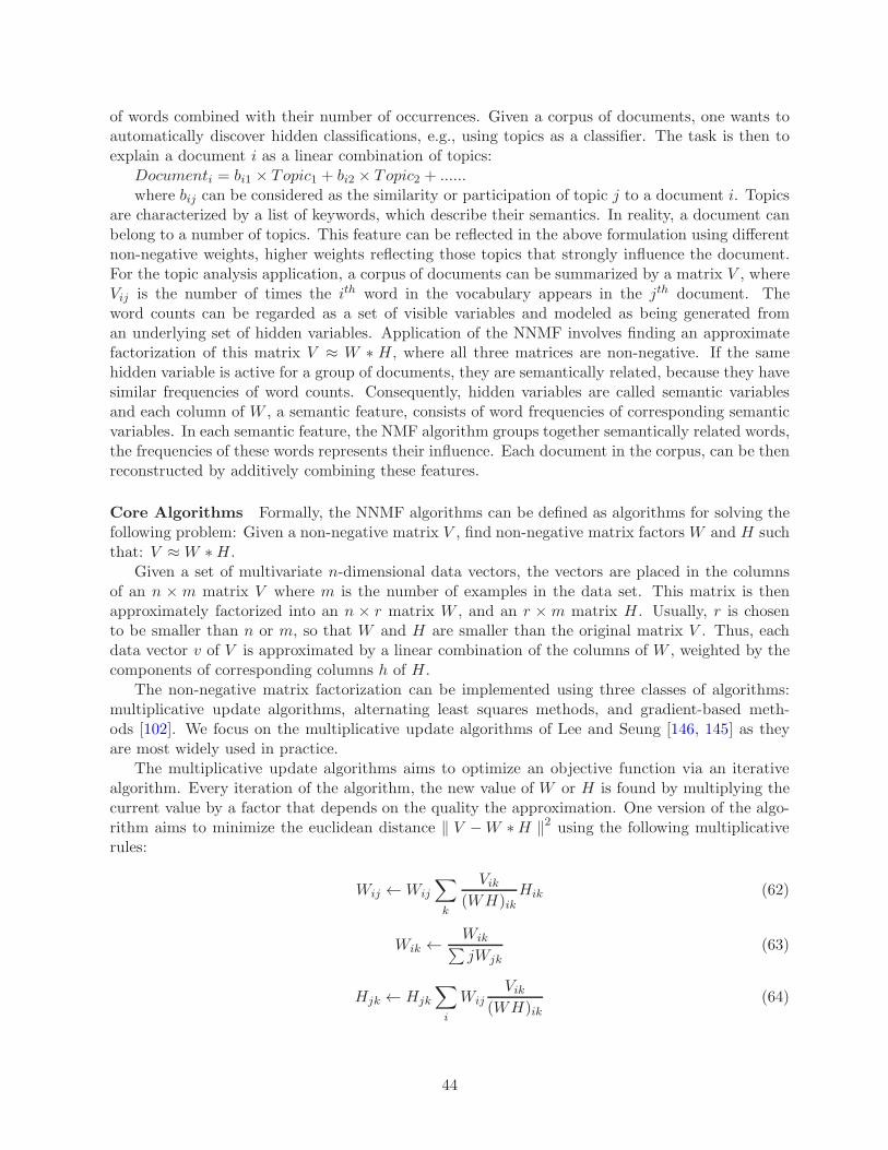
of words combined with their number of occurrences. Given a corpus of documents, one wants toautomatically discover hidden classifications, e.g., using topics as a classifier. The task is then toexplain a document i as a linear combination of topics:

Documenti = bi1 × Topic1 + bi2 × Topic2 + ......where bij can be considered as the similarity or participation of topic j to a document i. Topics

are characterized by a list of keywords, which describe their semantics. In reality, a document canbelong to a number of topics. This feature can be reflected in the above formulation using differentnon-negative weights, higher weights reflecting those topics that strongly influence the document.For the topic analysis application, a corpus of documents can be summarized by a matrix V , whereVij is the number of times the ith word in the vocabulary appears in the jth document. Theword counts can be regarded as a set of visible variables and modeled as being generated froman underlying set of hidden variables. Application of the NNMF involves finding an approximatefactorization of this matrix V ≈ W ∗ H, where all three matrices are non-negative. If the samehidden variable is active for a group of documents, they are semantically related, because they havesimilar frequencies of word counts. Consequently, hidden variables are called semantic variablesand each column of W , a semantic feature, consists of word frequencies of corresponding semanticvariables. In each semantic feature, the NMF algorithm groups together semantically related words,the frequencies of these words represents their influence. Each document in the corpus, can be thenreconstructed by additively combining these features.

Core Algorithms Formally, the NNMF algorithms can be defined as algorithms for solving thefollowing problem: Given a non-negative matrix V , find non-negative matrix factors W and H suchthat: V ≈W ∗H.

Given a set of multivariate n-dimensional data vectors, the vectors are placed in the columnsof an n × m matrix V where m is the number of examples in the data set. This matrix is thenapproximately factorized into an n × r matrix W , and an r ×m matrix H. Usually, r is chosento be smaller than n or m, so that W and H are smaller than the original matrix V . Thus, eachdata vector v of V is approximated by a linear combination of the columns of W , weighted by thecomponents of corresponding columns h of H.

The non-negative matrix factorization can be implemented using three classes of algorithms:multiplicative update algorithms, alternating least squares methods, and gradient-based meth-ods [102]. We focus on the multiplicative update algorithms of Lee and Seung [146, 145] as theyare most widely used in practice.

The multiplicative update algorithms aims to optimize an objective function via an iterativealgorithm. Every iteration of the algorithm, the new value of W or H is found by multiplying thecurrent value by a factor that depends on the quality the approximation. One version of the algo-rithm aims to minimize the euclidean distance ‖ V −W ∗H ‖2 using the following multiplicativerules:

Wij ←Wij

∑

k

Vik

(WH)ikHik (62)

Wik ←Wik

∑

jWjk(63)

Hjk ← Hjk

∑

i

WijVik

(WH)ik(64)

44

As the solution to the objective function is not unique, several constraints are added to thematrices W and H, e.g., the euclidean distance of the column vectors in W is 1 or an orthogonalityconstraint HTH = I [129, 65, 261].

When non-negative matrix factorization is used for document clustering, a non-negative matrixV (w, d), where w is the number of words, and d is the number of documents, is factorized into twofactors, W (w, c) and H(c, d), where c is the number of clusters. Each column of V contains wordcounts of for a particular document and each row of V contains the counts for a particular word.After factorization, document dj is assigned to a cluster k if Hkj = max∀iHij. Each element wij

of W represents the degree to which a word ti belongs to cluster j, while each element hij of Hindicates to which degree a document j belongs to a cluster i [129].

2.9.6 Further Reading

Basic idea [71, 158]; Algorithms: Naive Bayes [164, 158], Latent Semantic Analysis [61, 144, 143],String Kernel Functions [152], and Non-negative Matrix Factorization [145, 146, 102, 261, 129,65]; Packages: R [71], SPSS Modeler [117], STATISTICA [244], RapidMiner [208], Oracle DataMiner [193], and SAS [58]; Applications: [267, 46, 126, 152, 197, 212, 126, 78].

2.10 Monte Carlo Methods

The Monte Carlo method refers to a class of algorithms that employ repeated statistical samplingto compute approximate solutions to quantitative problems. These techniques are widely used forthe applications with inherent uncertainty, such as pricing of various financial instruments, or forsimulating systems with many coupled degrees of freedom, e.g., simulating behaviors of differentmaterials. While the Monte Carlo methods had been originally designed for solving problems withprobabilistic outcomes, they have also been applied to solve deterministic problems with infeasiblecomputational requirements, e.g., solving multi-dimensional definite integrals with a large numberof dimensions or with difficult boundary conditions.

The first application of the Monte Carlo methods was to understand behavior of nuclear reac-tions (e.g., neutrino travel patterns) [167]. Over the years, the Monte Carlo methodology has beenapplied to a wide array of applications domains including different physical sciences, engineering,finance, numerical analysis, and mathematical optimization [74]. Some well-known applications inthe physical sciences domain include liquid simulation and other molecular modeling problems, un-derstanding many-body interactions and quantum chromo dynamics (QCD) in quantum mechanics,simulation of protein membranes and other biological simulations, etc. Monte Carlo methods arebeing used for sensitivity analysis in process engineering or for simulating defects in VLSI designs.These methods are also being used in computational numerical analysis, e.g., for solving partialdifferential and integral equations, linear algebraic equations, and matrix inversion [90]. Perhapsthe most popular application of monte carlo methods is in financial engineering where they areextensively used for insurance risk modeling, pricing various types of options and derivatives, e.g.,European and American style options, mortgage-backed securities, and portfolio analysis (e.g.,calculating Value-At-Risk (VaR)) [81, 29].

2.10.1 Basic Idea

The Monte Carlo method is defined as an approach that represents an approximate solution ofa problem as a parameter of a hypothetical population, and using a random sequence of valuesto construct a sample of the population, from which statistical estimates of the parameter can beobtained [90]. For a problem, the Monte Carlo method repeatedly generates independent identically

45

distributed random variables from the same distribution as the problem, and then uses them ineither deterministic or stochastic model to compute the solution.

In its simplest formulation, the Monte Carlo method can be viewed as an approach that usesstatistical sampling to compute a numerical integral. For example, the first moment of the uniformdistribution over the interval [0, 1] can be computed via the integral

∫ 10 xdx, with the analytical

solution of 0.5. The Monte Carlo method estimates the integral value by using random variablesdrawn repeatedly from a uniform distribution, and then computing their mean [220]. Formally,for an integral Ψ =

∫ 10 f(u)du, the Monte Carlo method approximates a solution by introducing

a random vector U that is uniformly distributed in the region of distribution. After applying thefunction f to U, one gets a random variable f(U) with expectation

E[f(U)] =

∫ 1

0f(u)φ(u)du (65)

where φ is the probability density function of U. As φ equals 1 on the region of integration,the expectation matches the value of the determinist integral, Ψ =

∫ 10 f(u)du.

Ψ = E[f(U)] =

∫ 1

0f(u)du (66)

The random variable f(U) has mean Ψ and standard deviation σ. Ψ can be also viewed as aprobabilistic expression for the given integral. Thus, Ψ can be estimated with standard deviationσ using an unbiased estimator H = f(U[1]). To improve the approximation, one can generalize theestimator to accommodate a larger sample, U[1],U[2], . . . ,U[m], selected from the same distribu-tion. Applying the function f to each of these variables yield random variables, f(U[1]),f(U[2]),..f(U[m]), each with expectation Ψ and standard deviation σ. Then, the generalized estimator ofΨ, H, with standard error, σ√

m, can be defined as

H =1

m

m∑

k=1

f(U[k]) (67)

H is called the crude Monte Carlo estimator. The standard error of a Monte Carlo estimationdecreases with the square root of the sample size [211]. Secondly, the standard error is independentof the dimensionality of the integral. Unlike the conventional numerical integration approacheswhich suffer from the curse of dimensionality, the amount of work required by the Monte Carloapproach does not increase exponentially in the number of dimensions. Unfortunately, to improvethe estimation quality, the Monte Carlo approach usually requires a large number of samples. Oneway to improve the efficacy of the Monte Carlo methods is to use one of the variance reductionmethods, e.g., importance or stratified sampling. In general, the Monte Carlo methods are suitablefor software/hardware-based implementations that can efficiently generate random samples.

Sawilowsky [220] classifies applications of Monte Carlo methods into three types: (1) Usingstochastic techniques for solving deterministic problems, e.g., Monte Carlo integration for solvingmulti-dimensional integral problems, (2) Using stochastic techniques for solving problems withprobabilistic outcomes (e.g., pricing of financial instruments), usually referred to as the MonteCarlo Simulation, and (3) Using the Monte Carlo method as a tool for generating samples of aparticular probabilistic distribution. However, in many practical scenarios, this distinction getsblurred. Algorithms that emply the Monte Carlo methods use the following methodology:

1. Identify a probability distribution function that mimicks the problem under consideration(e.g., normal distribution for option pricing)

46

2. Generate samples from the probability distribution function using a pseudo-random numbergenerator

3. Pass the sample values through a deterministic or stochastic models (for simulation andsampling) to get the final result.

Irrespective of how the Monte Carlo methods are used in practice, all Monte Carlo implementa-tions rely on techniques to generate good random number generators. In practice, it is not possibleto generate pure random numbers, so Monte Carlo algorithms use pseudo-random good implemen-tation of a Monte Carlo method [220] number generators. Sawilowsky lists the following conditionsfor a good implementation of a Monte Carlo method:

• The pseudo-random number generator produces repeated values separated by a long period.

• The pseudo-random generator generates values that pass tests for randomness.

• The experiment uses enough samples so as to minimize the approximation errors.

• Proper sampling of the random values is used.

• The Monte Carlo approach is valid for the scenario being modeled.

• The model simulates the scenario in question.

2.10.2 Random Number Generators

Pseudo-random number generators (PRNG) refer to a class of computational algorithms that cangenerate a sequence of numbers that mimic random numbers. Usually, the numbers generated bythese algorithms repeat after a certain time which called the period of the PRNG algorithm. APRNG algorithm usually requires a seed number as its initial state. For a particular seed, thePRNG algorithm would produce the same sequence of numbers. The length of the seed determinesthe period of the PRNG algorithm: for a n-bit seed, the period is always less than 2n.

Most PRNG algorithms use bit manipulation and shuffling (e.g., the multiply-with-carry, xor-shift, subtract-with-borrow, etc.) combined with recurrence strategies to incorporate pseudo-randomness into the generated sequences. One of the widely used PRNG (used for implement-ing the rand() function in most compiler libraries) uses a recurrent generator, called the linearcongruential generator (LCG). The LCG is defined by the following recurrent relation:

Xn+1 ≡ (aXn + c) (mod m) (68)

where X0 is the seed, m, 0 < m is the modulus, a, 0 < a < m is the multiplier, and c,0 ≤ c < m, is the increment. Usually, the parameters c and m are relatively prime. The pseudo-random sequence Xn has period of at most m. However, the period of the LCG generator dependson the choices of the parameters and in practice, m is usually 232, 248, or 264. Unfortunately,random values generated from LCG suffer from serial correlation and hence, it is not ideally suitedfor the Monte Carlo computations.

The Mersenne Twister (MT) generator [162, 163, 214] has been designed applications for like theMonte Carlo methods that need random sequences with very long periods. For a k-bit word, the MTalgorithm generates integers with uniform distribution in the range [0, 2k−1]. The MT algorithm’speriod is chosen to be one of the Mersenne prime numbers: the most commonly used variant ofthe MT algorithm, MT19937 generates 32-bit pseudo-random integers over [0, 232] with the period

47

of 219937 − 1. The numbers generated by the MT algorithm are free of long-term correlations. TheMT algorithm uses a recurrence formulation that mimics operations of a large linear-feedback shiftregister via a matrix-vector multiplication over a finite binary field F2, in which the vector is builtusing bit manipulations (namely, xor and ordered concatenations) over initial integer seeds andcomputed values.

Another relevant PRNG family of algorithms is the Multiply-with-Carry approach [160] thatuses the following recurrence:

Xn = a×Xn−1 + (carry mod)232 (69)

where a can be any numbers for which both (a × 232) − 1 and (a × 231) − 1 are prime. Thecomputation is performed using modulo base b arithmetic, where b = 232. Along with its version, theComplimentary-Multiply-with-Carry algorithm [51], this approach can generate random numberswith very large periods.

2.10.3 Monte Carlo Variants

In practice, different variants of the original Monte Carlo algorithm are also used. One popu-lar variant, the Markov Chain Monte Carlo (MCMC) [166] is used for generating samples froma probability distribution by using a Markov Chain whose stationery distribution is the desireddistribution. The MCMC algorithm is used for solving multi-dimensional integral problems and ithas been also applied to scenarios that exhibit random walk behavior, e.g., in statistical physics orgraphics applications. Another version, the Quasi-Monte Carlo method, low-discrepancy samplesthat are deterministically chosen based on equi-distributed sequences. The low-discrepancy sam-ples often lead to faster solution time and/or higher accuracy. The Quasi-Monte Carlo methodsare used for solving multi-dimensional integration problems, e.g., pricing financial derivatives likeCollateralized Mortgage Obligation (CDOs) [200].

2.10.4 Further Reading

Basic idea [167, 90, 220, 166]; Algorithms [162, 163, 214, 51, 160]; Applications [167, 74, 90, 81, 29,200].

2.11 Mathematical Programming

In a mathematical optimization or programming problem, one seeks to find an optimal solutionfor a problem scenario as defined by its constraints using a mathematical formulation. Specifically,solution of a mathematical programming problem aims to minimize or maximize a real objectivefunction of real or integer variables, subject to constraints on the variables [104, 85]. The math-ematical programming approach is usually applied to cases where a closed-form solution is not(easily) found and one has to settle for the best available solution. It forms the cornerstone ofmethods used in operations research and other related disciplines like industrial engineering, so-cial sciences, economics, and management sciences. It has also been applied in a wide variety ofdomains including scheduling problems (e.g., transportation), manufacturing (e.g., steel produc-tion [66]), supply-chain management, product portfolio optimizations, workforce management, andproduct configuration selection.

2.11.1 Basic Idea

A mathematical program is an optimization problem of the form

48

Maximize f(x) : x ∈ X, g(x) ≤ 0, h(x) = 0 (70)

where X is a subset of Rn and is in the domain of the functions, f, g and h, which map intoreal spaces. The relations, x ∈ X, g(x) ≤ 0, and h(x) = 0 are called constraints, and the functionf is called the objective or cost function [104]. The domain X of the objective function is calledthe search space. A point x is feasible if x ∈ X and it satisfies the constraints: g(x) ≤ 0 andh(x) = 0. A point x∗ is optimal if it is feasible and if the value of the objective function is not lessthan that of any other feasible solution: f(x∗) ≥ f(x), for all feasible x (also called candidate orfeasible solutions). This description uses maximization as the sense of optimization. The problemcould be easily restated as a minimization problem by appropriately changing the meaning of theoptimal solution: f(x∗) ≤ f(x), for all feasible x.

The mathematical programming broadly covers approaches used for solving and using mathe-matical programs. It includes theorems to govern the form of the solutions, algorithms to seek asolution or ascertain none exists, formulations of problems as mathematical programs and theoremsabout quality of results, etc. In practice, mathematical programming approaches are classified ac-cording to the properties of the objective function, constraints, and candidate solutions. We nowdiscuss important classes of mathematical programming.

2.11.2 Linear Programming

Linear programming approach is a special case of convex programming in which the the objectfunction f is both linear and convex and the associated set of constraints are specified using onlylinear equalities or inequalities. Linear programming is used for modeling problems from operationsresearch such as network flow, production planning, financial management, etc. Canonically, thelinear programs can be expressed in matrix form as

Maximize cTx subject to Ax ≤ b x ≥ 0 (71)

where x represents the vector of variables to be determined, c and b are vectors of knowncoefficients and A is a known matrix of coefficients. The set of constraints, Ax ≤ b, form aconvex polytope and any linear programming method would traverse over its vertices to find apoint where the function, cTx, has the maximum (or minimum) value, if such point exists. Thisformulation of the linear programming problem is called the standard form. This form can beconverted into an augmented form that uses slack variables to convert inequalities into equalities inthe constraints. Every linear programming problem, referred as a primal problem, has an equivalentdual formulation. For example, the formulation presented in Equation 71 can be also expressed inits symmetric dual form as

Minimize bT y subject to AT y ≥ c y ≥ 0 (72)

The dual of a dual linear program is the original primal linear program and every feasiblesolution for a linear program (LP) gives a bound on the optimal value of the objective function ofits dual.

Most approaches for solving the linear programming problems explore the feasible region over aconvex polytope defined by the linear constraints of the problem. The simplex method [53] is oneof earliest, but still widely used, methods for solving LP problems. The simplex method constructsa feasible solution at a vertex of the polytope and then tests adjacent vertices by traversing apath on the edges of the polytope such that the objective function is improved or is unchanged.The simplex algorithm is very efficient in practice, requiring 2n to 3n iterations, where n is the

49

number of equality constraints and is known to run in polynomial time in certain random inputs.The worst-case complexity of the simplex algorithm is exponential in the problem size. Thisproblem was addressed by the Ellipsoid method [223, 245] that uses an iterative approach togenerate a sequence of ellipsoids whose volumes uniformly reduce at every step, thus enclosing aminimizer of the convex objective function. The Ellipsoid method was the first solution to the linearprogramming problems that ran in worst-case linear time. The Karmarkar’s algorithm [130, 245]that uses a interior-point projection method improves on the Ellipsoid method’s complexity boundsand runs in polynomial time for both average and worst cases. Unlike the simplex method, theprimal-dual (they can simultaneously optimize primal and dual versions of the feasibility functions)interior point methods construct a sequence of feasible points lying in the interior of the polytope,but not on the boundary of the polytope. For n variables and L bits used for encoding the input,Karmarkar’s algorithm requires O(n3.5L) operations as compared to O(n6L) operations requiredby the Ellipsoid method.

It has been shown that computations in Karmarkar’s primal-dual interior point method aresimilar to numerically solving the nonlinear equations for the unconstrained minimization prob-lem [79, 161, 245, 165, 256]. For example, the minimization problem (Equation 72) can be repre-sented as a family of unconstrained problems that use the logarithmic barrier function using thepositive barrier parameter µ:

B(x|µ) = f(x)− µ

n∑

j=1

log(xj) (73)

Lets x(µ) be the minimizer for B(x|µ). It can be shown that as µ → 0, x(µ) → x∗, where x∗

is the constrained minimizer. The set of minimizers, x(µ) is called the central trajectory (path).The following steps give an outline of the path finding barrier algorithm using a logarithmic barrierfunction [161]:

1. set k = 0. Choose µ0 > 0

2. Find xk(µk), the minimizer of B(X|µ) by using Newton’s method to solve the system of nequations in n variables:

∂B(x|µ)

∂xj=

∂f(x)

∂xj−

µ

xj= 0 for j = 1, · · · , n (74)

3. If µk < ǫ stop. Otherwise, choose µk+1 < µk.

4. Set k = k + 1 and go to 2.

This algorithm terminates as µk → 0 and xk(µk)→ x∗.Most existing implementations of the interior point algorithms follow the path-following based

approaches, e.g., the predictor-corrector approach [165].

2.11.3 Integer Programming

Integer programming (IP) family covers the set of linear programming applications that requirevalues of the unknown variables to be integer. If only some of the variables are required to beintegers, the problems are called mixed-integer programming (MIP) problems. Another versionof the integer programming problem, 0-1 or binary integer programming, requires values of theunknown variables to be either 0 or 1.

50

Integer programming formulations are used in a wide array of business problems that requireinteger solutions, e.g., in a capital budgeting situation, one wants to distribute a fixed amount ofmoney across different portfolios so as to maximize the profits. Integer programming problemsoften observed in scheduling scenarios, e.g., house building with workers with specific skills [111]and in assignment-related problems, e.g., airline fleet assignment for optimal utilization or profitmaximization [1]. Integer programming is also used in the distribution or network flow optimizationproblems that include transportation problems (e.g., optimizing the movement of goods from man-ufacturing plants to distribution centers to minimize shipping costs), to minimize cost or maximizeprofits), shortest-route problems (e.g., the traveling salesman problems (TSP)), and maximal flowproblems (e.g., to determine the maximum amount of flow (e.g., vehicles, network packets, or oil)can enter and exit a network system in a given period of time [7].

Multiple variants of the IP problems are generally NP-Hard and usually solved using two classesof techniques: cutting planes and branch-and-bound. The cutting-plane methods work by first solv-ing the linear programs generated via linear program (LP) relaxation (that drops the requirementthat the unknown variables must be integers) of the IP problems. The modified program is thensolved using traditional LP means (e.g., simplex method) to find a basic feasible solution. It isknown that the optimum solution to the relaxed IP problem is an upper bound for the optimalinteger solution. This solution represents a vertex of the convex polytope of all feasible points. Ifthis solution is integer-valued, then the process terminates. Else, the method finds a linear inequal-ity that separates the vertex from all feasible integer values. The linear inequality correspondsto an hyperplane that cuts the feasibility space (commonly called as a Gomory cut). A modifiedlinear program is then created by introducing the new inequality into the program. This modifiedprogram is then solved and the process repeats until the solution is found.

The branch-and-bound (BB) methods are a general class of search techniques that can be appliedto a variety of optimization problems including integer programming, quadratic programming, andcombinatorial optimizations [258]. The BB methods systematically enumerate feasible solutionsin the search space and prune them using upper and lower bounds of the cost function beingoptimized. The BB methods focus on the minimization version of the optimization problem (anymaximization problem can be easily recast in this formulation). In the first step, a set S of feasiblesolutions is split into smaller sets S1, · · · , Sn, whose union covers S. Each subset represents answerto a sub-problem of the original problem. The minimum value of the cost function f(x) over Sis min(v1, · · · , vn), where vi is the minimum of f(x) within Si. Usually, the sub-problems areenumerated using a search tree, whose root represents the original problem and each tree noderepresents a sub-problem. The next step, termed bounding, computes upper and lower bounds forthe minimum value of f(x) for each sub-problem. The final step prunes the candidate solutionsusing the computed bounds. If the lower bound for a solution set (that corresponds to a tree node)is higher than the upper bound of another solution set, then the former set can be discarded, and thesearch tree can pruned at that node. The pruning process is usually implemented by maintaininga variable to represent the global minimum upper bound. Then, any sub-problem that has a lowerbound higher than the global minimum can be safely discarded. This process recursively traversesthe tree until the candidate set of feasibility solutions contains one element or when the upperbound for a solution set matches the lower bound. Performance of the BB methods depend onsplitting procedure and how the bounds are computed.

The basic branch-and-bound methods can be generalized to incorporate LP relaxation tech-niques. The resultant approach, called branch-and-cut, first solves the relaxed form of the originalIP problem using the cutting plane method. Once the integer solution is found, the problem is splitinto two versions, one specifying that the variables are greater than the intermediate results, andthe other specifying that the variables are less than the intermediate results. These two modified

51

problems are again individually solved using the cutting plane methods. The process repeats untilan integer solution for all constraints is found. Thus, this method uses cutting and branchingthroughout the search tree. Another generalization, branch-and-price, also combines the branch-and-bound approach with LP relaxation [15]. In the branch-and-price approach, first a modifiedprogram with LP relaxation is solved using the simplex approach. Then to check the optimalityof the solution, additional constraints (or columns in Equation 72) are introduced using a pricingproblem. If there are new columns, the problem is re-optimized. If there are no columns to beintroduced, and the solution does not satisfy the integrity constraints, the problem is branched.Similar to the branch-and-cut approach, the branch-and-price algorithm uses pricing and branchingthroughout the search tree.

2.11.4 Combinatorial Programming

Combinatorial programming (or optimizations) cover methods that aim to optimize a cost functionbased on selection of objects from a set of objects [198]. Let N = 1, · · · , n be a set of objects andlet S1, S2, · · · , Sn be a finite collection of subsets. These subsets are characterized by inclusionand exclusion of objects based on certain conditions. Let each subset, Sk, be associated with a costfunction, f(Sk). The combinatorial optimization problem aims to select the subset of objects soas to maximize(minimize) the cost function. This formulation can be viewed as a special case ofinteger programming, whose decision variables are binary valued: x(i, k) = 1 if the ith element isin the kth set, Sk, otherwise, x(i, k) = 0 [104].

Broadly, the combinatorial programming approaches can be classified based on the problem for-mulation and the associated data structures. The most common problem formulations include pathtraversals, flow and circulation, matching and covering, trees and branching, cliques and coloring,matroids, packing (e.g., knapsack and cutting stock), sequencing/scheduling, and graph partition-ing/cuts [198, 224]. In practice, combinatorial optimization techniques are applied to a wide arrayof problems such as optimizing vehicle routing, VLSI circuit design, oil/gas pipeline design, steel/-paper manufacturing, and matching factories with markets via intermediate warehouses (i.e., thetransshipment problem).

Unlike linear programming, the feasibility space of the combinatorial algorithms is not con-vex; one needs to determine a global optimal point from several possible local optimal solutions.Although most combinatorial programming approaches are either NP-Hard or NP-Complete, inpractice, many of these approaches can be solved in reasonable time by either choosing alternativeformulations or exploiting specific features of a problem to compute its exact results [103]. Whilespecial cases of some problems can be solved in polynomial time, most common approaches forsolving combinatorial problems use either approximation algorithms that find a solution that isprovably close to the optimal in polynomial time or use heuristics that search the feasibility spaceto compute sub-optimal solutions.

The approximation approach has been shown to work for several combinatorial programmingproblems that include vertex cover, variants of the traveling-salesman problem (e.g., EuclidianTSP), set-covering, graph coloring, maximum clique and subset-sum [252]. The approximation al-gorithms are particularly suited for NP-Hard optimization problems, e.g., the bin packing problem,which may not have any efficient polynomial-time exact algorithms. For the NP-Hard problemsthat can be formulated via integer programming, linear programming relaxation is used to generatevariants which then can be solved using approximation algorithms. Alternatively, the combinatorialoptimization problems can be solved using heuristics that can search the space of feasibility solu-tions in a reasonable time, but provide no guarantee that an optimal solution can be found. Mostcommon combinatorial heuristics include greedy strategy, simulated annealing, search methods

52

(e.g., backtracking), stochastic optimizations, genetic algorithms, and tabu search.The greedy strategy is the simplest heuristics to be applied for combinatorial optimizations. This

strategy always follows locally optimal choice at every step to find the global optimum. This strategyassumes that the target problem exhibits optimal sub-structure, i.e., computing optimal solutionsto sub-problems leads to finding the global optimal solution. Unlike dynamic programming, whichreevaluates its decision at every step and if required, backtracks, the greedy strategy does notreconsider its decisions. This often results in the greedy strategy computing sub-optimal solutions.In spite of its disadvantages, the greedy approach is popular in practice mainly due to its fasterexecution.

The simulated annealing [132] approach takes inspiration from the metallurgical annealing tech-nique that uses repeated heating and slow, controlled cooling to form structurally strong materials.When a material is heated, the atoms get activated and randomly move through the states withhigher energy. Upon slow controlled cooling, they are more likely to find configurations with in-ternal energy lower than the original configuration. The simulated annealing algorithm appliessimilar approach for moving from a state to another. Given a state, the algorithm chooses anotherrandom state with a probability that is a function of the current state and a parameter calledtemperature. At each stage, the algorithm probabilistically decided whether to move or stay at theexisting state. The temperature is initially kept high and slowing reduced to zero as the algorithmprogresses. At higher temperature, there are more random changes; as the temperature reduces thesystem slowly reaches a steady state. Higher temperature increases the chances of state changesand protects the algorithm in getting stuck in the local minima, as in the greedy strategy. Note thatwhen the temperature is 0, the algorithm reduces to the greedy strategy. The execution time ofthe simulated annealing approach depends on the initial temperature and the associated annealingschedule. Often heuristics like the steepest descent are used to accelerate the execution.

The search algorithms are targeted for combinatorial formulations that use graphs or treesto represent the underlying computations, e.g., shortest path, maximum clique, etc. The searchalgorithms include exact enumeration approaches such as depth-first or breadth-first traversalsthat are used to solve combinatorial problem that search for sub-structures (e.g., cycles, cliques)within a graph model. Search algorithms also support search pruning methods like backtrackingand branch-and-bound approaches for optimizing cases where graphs or trees are used to maintainstate during execution of algorithms.

Simulated annealing can be considered as a special case of techniques, called stochastic op-timizations, that employ probabilistic approaches for either formulating or solving combinatorialproblems [233]. Other examples of stochastic optimizations include genetic or evolutionary algo-rithms and swarm intelligence. Genetic algorithms take an evolutionary view of the optimizationprocess: initial random population of solutions are chosen and from this set, a new set of solutionsis stochastically selected using a fitness function. This set and the fitness function are mutatedto create a new population for the next iteration (generation) of the algorithm. The algorithmsterminate when the number of generations reaches a limit or the fitness function reaches a suitablelevel. The swarm intelligence algorithms approach the optimization process as a de-centralizedself-organized system. In this formulation, several independent agents stochastically explore thefeasibility space and collaborate with other agents via shared state variables. The shared statehelps the agents to iteratively improve their selections; finally leading to emergence of the optimalsolution.

53

2.11.5 Constraint Optimizations

Constraint optimization (satisfaction) is a family of optimization problems that has a constantobjective function with a set of constraints that impose conditions on the solution variables. Asolution to a constraint satisfaction problem is a set of variables that satisfy all of the specifiedconstraints.

The constraint satisfaction problems (CSPs) are characterized by constraints that are definedover a finite domain [60, 9]. Most CSPs problems occur in scenarios that require solutions fromcombinatorial, logic programming or artificial intelligence (AI) fields. Examples of CSPs include:(1) the boolean satisfiability problem that aims to determine if variables of a given formula canhave values in the boolean domain such that the formula evaluates to TRUE (e.g., the 3-SATproblem), (2) the graph coloring problems, e.g., to determine the minimum number of vertex colorssuch that no two adjacent connected vertices share the same color, and (3) resource allocation andscheduling problems, e.g., the steel mill slab scheduling problem that computes the optimal weightand width of the steel slabs to minimize the losses. In practice, CSPs has been used for schedulingproblems, circuit layout in VLSI chips, DNA sequencing, production planning, computer vision,and computer games (e.g., sudoku) [174, 49].

Formally, a CSP problem involves a set of variables X1.X2, · · · ,Xn, where a variable Xi isdefined within a domain Di. The problem is associated with a set of constraints, C1, C2, · · · , Cm,such that a constraint Ci imposes a constraint on the possible values in the domain of some subsetof the variables. A solution to a CSP is an assignment of every variable with some value fromthe corresponding domain such that every constraint is satisfied [49]. In general, a constraint caninvolve n variables. Depending on a constraint’s arity, different optimization strategies can be used,e.g., expressing a constraint with arity > 2 using binary constraints. The CSP constraints can bealso expressed using the integer programming formulation: first, the multi-variate constraints areexpressed using equations, and a corresponding objective function is then defined. This formulationis termed as the constraint optimization problem, and its solution is the one that optimizes theobjective function.

The most common approach to solve the CSP problem is searching through different possi-ble alternative solutions. Unlike the generalized search algorithms used in AI, the CSP searchalgorithms can use heuristics that exploit the problem structure and also perform search in anyorder. Searching in a CSP algorithm involves first choosing a variable and assigning a value forit. If the search states are represented as a tree, a variable would be assigned a node with edgesthat represent possible values assigned to that variable. With n variables, one gets a search treeof depth n, where a path from root to the leaves represents a search state with an ordering of nvariables with associated values. Performance of any search algorithm depends on ordering of thevariables and choices of their values. Two commonly used heuristics for variable ordering includethe minimum-remaining values (MRV) that chooses a variables with the least number of possiblevalues from its domain and the degree heuristic which chooses a variable that is involved in mostconstraints. Once a variable is selected, the next step is to choose its value. The most commonheuristic, LCV (least constraining value) is to choose a value that eliminates fewest options for theother variables.

Most CSP algorithms use depth-first search to traverse the search tree. Often, the traversalsreach a node where a node cannot be updated as the domain is empty. In such cases, the searchalgorithms backtrack to the previous assignment (i.e.. a node at a higher level in the search) andrestart the search with a new assignment. Further, value assignments to the search tree nodes aremade such that the assignments are consistent as per the associated set of constraints. Consistencycan be maintained using the forward consistency approach that given a value assignment, can

54

predict the set of assignments that can lead to a failure. Thus, the forward consistency approach canbe used for intelligently pruning search paths. The forward consistency approach is a special caseof k-consistent constraint propagation that ensure that assignment to any subset of k− 1 variablesallows a consistent assignment to the kth variable. Other approaches for preserving consistencyinclude node consistency that checks consistency of a single assignment, arc consistency that checksconsistency for any pair of variables, X and Y , for both assignment orders (i.e., X followed by Y , andvice versa), and path consistency that uses groups of 3 variables to validate value assignments [49].

One of most widely used CSP search algorithms is the A* algorithm [185, 173]. The A* algo-rithm uses the best-first strategy to choose the next search node to traverse. However, unlike thetraditional greedy best-first strategy, the A* algorithm uses a heuristic cost function that encodes(1) the cost of reaching the current node, n, from the starting node g(n), and (2) an admissible(i.e., does not overestimate) estimate of the cost of reaching the goal from the current node, h(n).The cost function f(n) can be then computed as g(n) + h(n). The A* algorithm for any noden, computes its cost function f(n), and adds it to a priority queue with the priority f(n). Forevery child n′ of the node n, the A* algorithm computes its cost function f(n′), and adds it to thepriority queue if n′ wasn’t traversed before or it was analyzed with a higher cost. Once a node iscompletely expanded (i.e., its children are traversed), it selects the node with the lowest priorityfrom the queue, and the process repeats. The algorithm terminates when the goal is reached. TheA* algorithm only considers acyclic paths and since the search tree has only finite acyclic paths,the A* algorithms is designed to terminate. If the A* algorithm implementation uses an admissibleheuristic, then it is guaranteed to identify optimal path. The time complexity of the A* algorithmdepends on the heuristic being used in the cost function. In the worst case, it can run in expo-nential time. As A*’s runtime is O(number − of − states), it can consume lots of memory. Formemory-constrained scenarios, memory bounded search algorithms like the iterative deepening A*(IDA*) are preferable [173].

2.11.6 Nonlinear Programming

The nonlinear programming (NLP) can be viewed as a generalization of different mathematicalprogramming formulations. In an NLP formulation, either or both the objective function or theconstraints can be nonlinear. An NLP problem has the following form: minimize f(x), subjectto gi(x) = 0, for i = 1, . . . ,m1 and hj(x) ≥ 0, for j = m1 + 1, . . . ,m, m ≥ m1 ≥ 0. Dependingon the non-linearity, multiple special cases arise. Foe example, a scenario where the objectivefunction is non-linear, but the constraint functions g and h are linear, is called a linearly constrainedoptimization. If the objective function and the constraints are linear, an NLP problem reduces to alinear programming problem. When only the objective function is quadratic, the problem is termedquadratic programming. If the objective and constraint functions are defined over a convex set,the problem is called convex optimizations [28]. Finally, when both the objective function andconstrains are non-linear, the problem is called unconstrained optimization [180].

As many situations that we encounter in everyday life do not behave linearly (e.g., doubling thenumber of people does not guarantee that the project would be completed in half the time), NLPmodels have become prevalent in practice. Nonlinear programming has been routinely used to solveboth discrete and continuous optimal control problems. Nonlinear programming models have beenapplied to determine how to clean up pollution in the underground water system; for designingtrusses that can withstand different loads, for choosing a portfolio investment mix that maximizesreturn while minimizing risks, for choosing the width and length of devices in an electronic circuit,for modeling traffic patterns to capture congestion and travel times, and for choosing resources tosatisfy project deadlines [179].

55

The difficulty in solving an NLP problem arises from the fact that NLP problems have non-convex object function or constraints. Such problems can have multiple feasible regions and multiplelocally optimal points within each regions. Consequently, the non-convex NLP problems can ex-hibit solutions with local optima: they are spurious solutions that satisfy the requirements on thederivatives of the constraint functions. To determine if an NLP problem is infeasible (e.g., the ob-jective function is unbounded) or a solution is the global optimum can require time exponential inthe number of variables and constraints. The complexity of solving an NLP problem varies accord-ing to its type: in general, problems with convex objective function or constraints (e.g., quadraticprogramming) are easiest to solve, while problems that aim to find the global optimal are muchharder to solve.

A quadratic programming (QP) problem can be formalized as

Minimize f(x) = cx+1

2xTQx subject to Ax ≤ b and x ≥ 0 (75)

where c is an n-element row vector representing the coefficients of the linear objective function,Q is a n× n symmetric matrix representing the quadratic coefficients. The m× n matrix A, alongwith the n-element column vector x of decision variables and the m-element column vector b ofcoefficients, represent the linear inequality constraints (a QP problem can optionally have equalityconstraints as well). If the objective function is strictly convex, i.e., the matrix Q is positive definite(negative definite for the maximization case), then the QP problem has an unique local minimumwhich also in the global minimum. In general, a QP problem can be evaluated for feasibility of aglobal optimal solution by checking the Karush-Kuhn-Tucker (KKT) conditions [83]. Most commonQP problems (e.g., portfolio optimization) can be viewed as a special case of the second-order coneprogramming and can be solved using extensions to the Simplex or Interior-point methods. In caseswhere the nonlinear function is smooth, i.e., its derivatives with respect to each decision variable(function gradient) are continuous, gradient methods can also be applied.

The convex optimization problem is an NLP problem in which the objective and constraintfunction satisfy the following convex inequality [28].

fi(αx+ βy) ≤ αfi(x) + βfi(y) (76)

where x, y ∈ Rn and α, β ∈ R with α + β = 1, α ≥ 0, β ≥ 0. While there are no algorithmsspecifically designed for solving the convex optimization problems, most convex optimization prob-lems are easier to tackle as (1) any local optimum is necessarily a global optimum, (2) one caneasily check the infeasibility of the objective function, and (3) efficient numerical solutions exist forsolving large problems [100]. In practice, well-known methods like the Interior-point or gradientmethod and its variants are used to solve the convex optimization problem.

Finally, the global optimization aims to find the absolutely the best solution for the objectivefunction under given constraints. As mentioned earlier, the worst case complexity of the globaloptimization methods grows exponentially with the problem size and constraints. In spite of theexecution cost, there are scenarios where an exhaustive search for the best solution is indispensable.Many well-known problems from from graph theory (e.g., the traveling salesman or maximum cliqueproblem), packing, scheduling, chemistry (e.g., the chemical equilibrium problem), verification(computer-assisted proofs), protein folding, robotics, and even numerical analysis (nonlinear leastsquares fitting problem) use the global optimization approach [181]. In practice, most solutions usecomplete methods that aim to achieve global optimum with certainty, assuming exact computationsand indefinitely long run time, but within a finite time, determine that an approximate globaloptimal has been found [181]. Most complete algorithms use the branching principle that recursively

56

splits the original problem into subproblems, that are addressed separately. The search spacecan be controlled either by using the branch-and-bound approach or by propagating constraints.Alternatively, the original problem can be converted via outer approximation of the constraints andunderestimation of the objective function to generate a relaxed version that is convex and can besolved by convex optimization methods.

2.11.7 Further Reading

Basic idea [104, 85, 180]; Algorithms: Linear Programming [53, 223, 245, 79, 161, 245, 165, 256, 165],Integer Programming [15], Combinatorial Programming [198, 224, 103, 252, 132, 233], ConstraintOptimizations [60, 9, 185, 173], Non-linear Programming [28, 180, 83, 181]; Packages: IBM ILOGCPEX [111], COIN-OR [45], Gurobi [87]; Applications [66, 111, 1, 7, 174, 49, 198, 224, 11];

2.12 On-line Analytical Processing (OLAP)

On-line analytical processing or OLAP refers to a broad class of analytics techniques that processhistorical data using a logical multi-dimensional data model [43, 44, 39]. Over the years, OLAPhas emerged to become the key business intelligence (BI) technology for solving decision supportproblems like business reporting, financial planning and budgeting/forecasting, trend analysis andresource management. OLAP technologies usually operate on data warehouses which are collec-tions of subject-oriented, integrated, time-varying, non-volatile, historical collection of data [39].Unlike on-line transaction processing (OLTP) applications that support repetitive, short, atomictransactions, OLAP applications are targeted for processing complex and ad-hoc queries over verylarge (multi-Terabyte and more) historical data stored in the data warehouses.

2.12.1 Basic Idea

OLAP applications are targeted for knowledge workers (e.g., analysts, managers) who want to ex-tract useful information from a set of large disparate data sources stored in the data warehouses.These sources can be semantically or structurally different and can contain historical data consol-idated over long time periods. OLAP workloads involve queries that explore relationships withinthe underlying data and then exploit the acquired knowledge for different decision support activi-ties such as post-mortem analysis/reporting, prediction, and forecasting. The OLAP queries tendto invoke complex operations (e.g., aggregations, grouping) over a large number of data items orrecords. Thus, unlike the OLTP workloads, where transaction throughput is important, querythroughput and response times are more relevant for OLAP workloads. Thus, an OLAP systemneeds to support a logical model that can represent relationships between between records suc-cinctly, a query system that can explore and exploit these relationships, and an implementationthat can provide scalable performance.

2.12.2 Logical Data Model

Most OLAP systems are based on a logical data model that views data in the warehouse as multi-dimensional data cubes. The multi-dimensional data model grew out of the two-dimensional array-based data representation popularized by the spreadsheet applications used by business analysts [39,84, 96]. The data cube is typically organized around a central theme, e.g., car sales. This themeis usually captured using one or more numeric measures or facts that are the objects of analysis(e.g., number of cars sold and the sales amount in dollars). Other examples of numerical measuresinclude budget, revenue, retail inventory. The measures are associated with a set of independent

57

dimensions that provides the context. For example, the dimensions associated with the car salesmeasure can include the car brand, model and type, various car attributes (e.g., color), geography,and time. Each measure value is associated with an unique combination of the dimension values.Thus, a measure value can be viewed as an entry in a cell of a multi-dimensional cube with aspecified number of dimensions.

In the multi-dimensional OLAP model, each dimension can be further characterized using aset of attributes, e.g., the geography dimension can consist of country, region, state, and city.The attributes can be viewed as sub-dimensions and can themselves be related in a hierarchicalmanner. The attribute hierarchy is a series of parent-child relationships that is specified by the orderof attributes, e.g., year, month, week, and date. A dimension can be associated with more thanone hierarchy, e.g., the time dimension can be characterized using two hierarchies: year, quarter,month, and date, and year, quarter, week, and date. The parent-child relationship represents theorder of summarization via aggregation: the measure values associated of a parent are computedvia aggregation of measures of its children. Thus, the dimensions, along with their hierarchicalattributes, and the corresponding measures, can be used to capture the relationships in the data.

2.12.3 OLAP Queries

Typical OLAP analytics queries perform two main functions: reporting and presentation. Report-ing involves organizing dimensions and performing computations on the corresponding measures.Presentation involves selecting dimensions and measures from the original or computed versions ofthe data, and preparing them for display. Functionally, OLAP queries can be classified into what-now (post-mortem analysis), what-if (prediction), and what-next (forecasting). To support theseanalyses, an OLAP engine supports a number of operators. Some of the key operators include:

• Group-by: The group-by operation collates the measures as per the unique values of thespecified dimensions. For example, in case of the car sales scenario, one may want to analyzethe impact of car color on the sales numbers by organizing the sales data according to thecolors. The collated values can then be sorted in increasing or decreasing order. In caseswith multiple dimensions, data can be collated across multiple dimensions in some order,e.g., grouping the sales by car brand and color would first collate sales of cars as per themake and within the make, the sales would be organized as per the car color (for differentcar types, e.g., passenger cars, SUVs, etc.).

• Slice and dice: The slice and dice operation involves reducing the dimensionality of thedataset by taking a projection of the data on a subset of dimensions for selected valuesof the other dimensions. For example, one can slice and dice the car sales data for a carbrand (e.g., Toyota) for particular region (e.g., Eastern United States) for the winter season.The slice and dice operation creates another cube that is a projection of the original cube.

• Pivoting: The pivoting or rotating operation re-orients the original cube to visualize the datausing new relationships. For example, an analyst may want to analyze the car sales using citiesand car brands as the pivot dimensions. The pivoting operation would then create anothercube with cities as one dimension and car brands as the other dimension. The correspondingmeasures, car sales in units and dollars, would be re-computed via summarization in the newdimensions. Thus the pivoting operation creates another cube from the original dataset withnew dimensions and hierarchies.

• Rollup and Drill-down: The rollup and drill-down operators support aggregation across hi-erarchies within one or more dimensions. The aggregation operation can invoke different

58

computational operators, e.g., sum, max or min. For example, the car sales measures canbe aggregated up within the time dimension (e.g., day, week, month, and year) to computethe total sales per every year and over all years maintained in the data warehouse. This sumcan then be rolled over another dimension, e.g., geography, to find out sales over years ineach geography, and finally over all geographies and years in the data warehouse. The orderof rollup is specified by the analyst and it results in different intermediate sub-totals. Thedrill-down operation produces the opposite effect: given a summarized value, the drill-downoperation finds out the contributions of the hierarchies and dimensions.

• Cube: The cube is a generalization of the roll-up operator, i.e., it computes summarization ofmeasures across all hierarchies and dimensions in the data warehouse. For example, the cubeoperator can calculate sales of a car brand over all car types, car colors, and over geographies,and time dimensions. The order of the aggregation can specified by the analyst. The cubeoperator follows the all possible relationships as defined by the lattice of relationships amongthe hierarchies [84]. The result of a cube operation is a list of summarizations across allhierarchies, dimensions, and finally over the entire dataset.

• Computational Operators: OLAP analysis involves invoking a variety of analytical functionson measure values. The OLAP analytical functions can be broadly classified into aggregation,scalar, and set functions. The aggregation functions operate on a set of values to computea scalar result. Examples of the aggregation functions include sum, average, correlation,count, etc. The scalar functions operate on individual measure values and compute a newset of measures. The set functions operate on a set of measure values and return a newset. Examples of the set functions include sorting, predicated selection, and ranking. Thesefunctions can be either user-defined or pre-defined by the underlying system.

2.12.4 OLAP Servers Implementations

In practice, the multi-dimensional OLAP model is usually implemented using one of the threeapproaches: Relational OLAP (ROLAP), Multi-dimensional OLAP (MOLAP), and Hybrid OLAP(HOLAP) [39].

• ROLAP: In the ROLAP approach, a relational database system is used for storing and pro-cessing data in the multi-dimensional OLAP model. The data warehouse is implemented asrelations stored in tables and queried using SQL-based OLAP queries.

Most relational data warehouses build the multi-dimensional OLAP models from data storedas dimension and fact tables. These tables are related via referential relationships. The mostcommon schema used for representing a OLAP cube is the star schema. In this approach,there is a single fact table containing the measures and a single table for each dimension ofthe cube. Each dimension table consists of attribute columns that correspond to attributes ofthe dimension. The fact table is related to the associated fact tables via the primary-foreignkey relationships. The star schema does not provide support for attribute hierarchies. Arefinement of the star schema called the snowflake schema enables attribute hierarchies byusing normalized dimension tables. Complex data warehouses can require multiple fact tablesto share dimension tables. This schema is called a fact constellation.

In addition to the dimension and fact tables, the relational database can also maintain ma-terialized views to represent pre-computed OLAP data. For example, a materialized viewcan represent summarized results of a rollup operation over a dimensional hierarchy. The

59

materialized view can be stored using separate shrunken dimension and fact tables or canbe represented in the same table space using an additional attribute, e.g., a level field thatrepresents the degree of summarization [39].

The relational database also provides in-built support for querying OLAP data via extensionsto the SQL language [37]. Specifically, SQL enables key OLAP operations using clauses likeROLLUP, CUBE, GROUP BY, and ORDER BY. The slice and dice operation can be implementedusing the SQL WHERE clause. Finally, SQL supports many computational operators natively,e.g., sum, min, max, average, etc. Additional computational operations can be implementedby invoking user-defined functions (UDFs).

• MOLAP: The MOLAP approach stores and processes the multi-dimensional OLAP cubesas multi-dimensional arrays. In most cases, the MOLAP cubes are sparse multi-dimensionalarrays that are stored using specialized data structures to optimize data access costs. TheMOLAP approach is suitable for scenarios that process low-dimensional data, have repeatedqueries that touch the same data, and require fast query performance. Examples of MOLAP-based systems include the SAP Hana [215], IBM PowerCube and TM1 [110] and MicrosoftSQL Server OLAP Services [170].

Data stored in the MOLAP fashion is queried using languages that can express data accessusing the multi-dimensional array model. An example of such languages is Microsoft’s Multi-dimensional Expressions (MDX) language [170]. MDX views the OLAP data as an instance ofa multi-dimensional cube. A basic MDX query follows the SELECT FROM WHERE structure ofthe SQL queries. Logically, a MDX query selects different axis from a data cube, with optionaldimensional slicing specified by the WHERE clause. In MDX, a member is an item in a dimen-sion representing one or more occurrences of data. The basic unit of representation in a MDXquery is a tuple that can encompass members in multiple dimensions as well members fromthe same dimension. MDX organizes tuples into sets which are ordered collections of zero, oneor more tuples. The set dimensionality is determined by the dimensionality of the containedtuples. MDX provides explicit syntactical support for navigation within and across OLAPcube dimensions and hierarchies using members, tuples, and sets, e.g., MEMBERS, CHILDREN,and DESCENDANTS. Finally, MDX provides support for a set of computational functions, e.g.,sum, min, max, and average.

• HOLAP: The hybrid OLAP strategy uses a combination of relational amd multi-dimensionalOLAP implementations to store and process OLAP data. There are two ways for partitioningdata between ROLAP and MOLAP stores: the first strategy stores the materialized view fora query workload in the MOLAP format and maintains the raw, detailed data in the ROLAPformat, while the second stores some section of the data (e.g., most recent or most commonlyused) in the MOLAP format, while maintaining the remaining data in the ROLAP format.Examples of systems that use the HOLAP approach include OLAP servers from Microsoft,Oracle and SAP [33].

2.12.5 Further Reading

Basic Idea [43, 44, 39, 84], Algorithms [39, 84, 96, 259]; Packages: Microsoft SQL [169, 170], IBMDB2 and Cognos TM1 [110, 37], Oracle [192], Teradata [240], HP Vertica [253], IBM Netezza [116],SAP [215, 122] and Palo [125]; OLAP Applications [33, 39].

60

2.13 Graph Analytics

Graphs and related data structures (e.g., trees and directed-acyclic graphs (DAGs)) form the fun-damental tools used for expressing and analyzing relationships between entities. Relationshipsmodeled by graphs include associations, hierarchies, sequences, positions, and paths [36, 13, 184].Graphs have been used in a wide array of diverse application domains: from biology, chemistry,pharmacology, linguistics, economics, operations research to different problems in computer science.

2.13.1 Basic Idea

Formally, a graph G = (V,E) is described using a set of vertices (or nodes) V and the edges Ethat connect them. The graph vertices or edges can be weighted, and the edges can be directedor undirected. Graph vertices can also support additional attributes, e.g., a color. Usually, thegraph is traversed in a pattern which is determined by either the graph characteristics or externalconstraints. This basic formulation of the graphs can be used for building complex data models.For example, molecular structure of chemical compounds is usually represented using graphs whosenodes represent atoms and edges represent bonds; a node- and edge weighted graph can represent atransportation system between cities of a region, where the node weight represents city populationand edge weight represents transportation density; a tree can represent an XML document withnodes the represent XML elements and have edges that connect them to attributes or hierarchical orsibling elements (in general, a tree is used to represent any dataset with hierarchical relationships);a program task graph in which the nodes represent tasks and edges represent task dependencies,and node colors denote tasks can be executed concurrently, and finally, entities (e.g., webpages orsocial network contacts) linked on the internet are usually modeled by a graph in which the nodesrepresent entities and edges represent connections [206]. Other applications of graphs includebiological modeling, sociology (e.g., social network analysis), linguistics (e.g., expressing languagesyntax and semantics), electrical circuit design, combinatorial optimizations (e.g., flow problems),and neuroscience (e.g., modeling brain’s cognitive connections [249]).

Graph analytics refers to a class of techniques that either use graph models to solve a prob-lem (e.g., the traveling salesman and other optimization problems), or to analyze and exploitinherent graph structures of a problem (e.g., identifying sub-graphs with a well-defined structure,motifs [172], from graphs representing chemical compounds). Broadly, the graph algorithms can beclassified into three overlapping categories: structural algorithms that analyze and exploit differenttopological properties of a graph, traversal algorithms that navigate different paths in a graph,and pattern-matching algorithms that find instances of different graph patterns (e.g., cycles) in agraph. These algorithms are characterized by how the graph data is interpreted and analyzed, andhow the graphs are represented. Common graph representations include directed and undirectedgraphs, graphs with weights on the edges and vertices, rooted graphs, commonly called trees, andtheir variants. A directed graph is usually referred as the digraph; its most popular variants includedirected acyclic graph (DAG) and network graph which is a digraph with weighted edges. In prac-tice, the graphs are represented using two different formulations: the first one enumerates the graphedges using lists, while the second uses matrices to capture the graph structure. The list-baseddata structures include adjacency list that colocates a vertex with its neighbors (i.e., vertices withdirect connections), and incident list that lists all edges as pairs or tuples (for directed graphs).The list-based representation is popular in the algorithms that navigate the graph structure. Thematrix formulation is used to provide a concise representing of different structural attributes of agraph, e.g., connectivity, weights, direction, etc. In most situations, the graph matrices are sparseand are implemented using compact array-based data structures.

61

2.13.2 Structural Algorithms

Graph structural algorithms, commonly known as network analysis algorithms, analyze symmetricand asymmetric relationships between networked entities by exploring structure of the underlyinggraph. Usually, the networked data is represented via digraphs or networks [184, 13, 36]. Thesenetworks can be structurally classified into the following categories:

• Small-world Networks: The small-world network is a type of digraph in which distance be-tween any two randomly chosen vertices grows proportional to the logarithm of the totalnumber of vertices in the network [255]. In other words, in the small-world network, mostvertices may not be directly connected to each, but they can reached from each other in a smallnumber of steps. These graph exhibit vertices (hubs) with large degrees (high connectivity)and sub-networks with high clustering coefficients.

• Scale-free Networks: In the scale-free network, the degree distribution follows the powerlaw [14]: the fraction P (k) of vertices with k connections to other nodes, for large values ofk, has the following characteristics: P (k) ∼ ck−γ , where 2 < γ. The scale-free network hasthe following properties: (1) it exhibits fault tolerant behavior as most nodes have smallerconnectivity and probability of all hubs failing is very low, (2) clustering coefficient of ascale-free graph also follow power law. That means, vertices with low degrees are a partof a dense sub-graph which are connected via high degree nodes (hubs). Many small-worldnetworks exhibit scale-free properties, but there are scale-free networks that do not have thesmall-world properties.

It has been observed that graphs exhibited by many real-world problems exhibit small-world orscale-free properties. Examples include sociological networks (e.g., actors or research collaborators),protein regulatory networks, neuron network in the visual cortex of the brain, cell phone call graphs,transportation (air and road) networks, power grids, internet connectivity graph, and web-pageconnection graph [249, 35].

Graph structural algorithms are designed to understand and exploit inherent abstract structuralproperties of a network. Such structural information can be used for different purposes, for example,telecom companies can use the structural information of the call graphs to identify customers mostlikely to switch carriers (also called churn analysis) [178, 54, 210]. The following list enumeratessome of the important properties of a network:

• Order and Size: For a graph, the number of vertices is its order and the number of edges isits size.

• Degree: For a graph, the degree (or valency) of a vertex is the number of edges incident onthat vertex. For a digraph, the degree can be further classified as the in-degree which is thenumber of edges incident on a vertex, and the out-degree is the number of edges emanatingfrom a vertex.

• Distance: For a graph, the distance between any two vertices is a number of edges (or thelength) in the shortest path between those vertices.

• Diameter: For a graph, its diameter is defined as the longest of all shortest paths betweenpairs of its vertices (or the maximum among all distances).

• Girth: The girth of a graph is the length of the shortest cycle in the graph.

62

• Connectivity coefficients: For a graph, the vertex (edge) coefficient represents the minimumnumber of vertices (edges) whose removal will disconnect the graph.

• Chromatic numbers: The chromatic numbers measure the number of graph structures (e.g.,edges, vertices, faces) that have different color under the constraint that no two connectedstructures (e.g., edges or vertices) have the same color.

• Clustering coefficients: The clustering coefficient of a graph is a measure to represent howvertices of a graph tend to cluster together. For a vertex, the clustering coefficient is calculatedas the ratio of the number of edges in its neighborhood (defined as a set of vertices directedconnected to the vertex) to the number of all possible edges in the neighborhood.

• Centrality: The centrality measure determines the importance of a vertex in a graph. Thereare four different types of centrality measures: degree, closeness, betweenness, and eigenvec-tor. The degree centrality of a vertex is the its degree normalized with the total numberof edges in the graph. The closeness measure for a vertex is defined as the mean geodesicdistance (i.e., the shortest path) between that vertex and all other vertices in that graph. Thebetweenness measure of a vertex is the fraction of the number of shortest paths of a graphpassing through that vertex against the total number of shortest paths in that graph. Theeigenvector centrality is a recursive version of the degree centrality: a vertex has a high valueif it is connected to another vertex with the high value (i.e., connections to other highly ratedvertices value more than connections to low rated vertices).

One representative example of the network analysis algorithms is the eigenvector centralityalgorithm [183]. The Google PageRank algorithm uses its variant [196, 206] for ranking web pages.It has also been applied to other domains such as studying fMRI brain scans [154]. The eigenvectorcentrality assumes that not all connections between vertices are equal. Specifically, connections withimportant vertices will lend a vertex more influence than connections to less important vertices.The eigenvalue centrality algorithm uses the adjacency matrix A to represent a graph: the entryAij is 1 if vertices i and j are connected. For undirected graphs, the adjacency matrix is symmetric,but for directed graph the matrix is asymmetric. The adjacency matrix can be generalized to storeedge weights as well. If xi is the centrality of a vertex i, then xi can be computed as an average ofthe centralities of i’s neighbors:

xi =1

λ

n∑

j=1

AijXj (77)

where λ is a constant. Defining the vector of centralities x = (x1, x2, . . .), we cab rewrite theequation in the matrix form as

λx = Ax (78)

Hence, the centrality vector x can be computed as an eigenvector of the adjacency matrix witheigenvalue λ. The eigenvector computations can use any of the known eigenvector algorithms, e.g.,the power iteration algorithm. In general, there can be many different eigenvalues for which aneigenvector exists. However, to compute positive centrality values, only the eigenvector correspond-ing to the largest eigenvalue is needed [183]. The ith entry in the eigenvector gives the centralityvalue of the ith vertex. The eigenvector centrality captures both the number and quality of itsconnections: a vertex with a small number of high-quality contact may get higher score than avertex with a higher number of connections. The eigenvalue approach used in this algorithm is anexample of the spectral graph methods [6, 63].

63

2.13.3 Traversal Algorithms

The second class of graph algorithms involves traversing edges of a graph to find solution of theassociated problem. Graph traversal algorithms operate on graphs that either capture the structureof some underlying physical network (e.g., roads, pipes, etc.) or capture the abstract model of aproblem (e.g., a tree representing an XML document, or a graph representing cities and distances ina traveling salesman problem). The traversal algorithms are used to solve: (1) route problems whichaim to optimize path lengths under different constraints, (2) flow problems that investigate flowof material (e.g., oil, gas, cars, etc.) over a network that is represented by the underlying directedgraph, (3) coloring problems that label graph elements (e.g., vertices) to satisfy certain constraints,and (4) searching problems that find a problem solution by traversing vertices which encode theproblem states. Unlike the structural algorithms where in many cases, analytical solutions arecomputable via matrix formulation, problems addressed using traversal algorithms are notoriouslycomplicated to solve - many of them are NP-Complete, and thus the algorithms must make extensiveuse of heuristics.

The route problems focus on optimizing graph traversals such that certain conditions are met,e.g., the first route problem, Euler’s Seven Bridges problem, investigates if it is possible to visit everyvertex of a graph by traversing each edge only once. A version of this problem aims to determine ifthere is exists a path or cycle in a undirected graph that visits each vertex exactly once (HamiltonianPath problem). Another version, the minimum spanning tree, tries to find a tree that spans (i.e.,connects all vertices) an entire graph (directed or undirected) with the minimum cost: path lengthor weights if the edges have weights. These problems have several practical applications, e.g., theminimum spanning tree (MST) is used to lay out electric power generation grid and the Hamiltonianpath problem is a special case of the traveling salesman problem. While efficient polynomial greedyalgorithms exist for the MST problem (e.g., Kruksal, Prim, and Boruvka), the Hamiltonian pathproblems are NP-complete, and need heuristics to solve even its simplest variants. Most solutionsto the route problems exploit non-matrix based data structures (e.g., queues, lists) to navigate thegraphs.

The second type of traversal algorithms focus on various notions of the network flow: theunderlying graph is a directed graph whose each edge has a capacity that limits the amount offlow over that edge. Each node of the graph receives an amount of flow, and except for specialcases (source and sink nodes), for every node, the amount of incoming flow must match the amountof outgoing flow. The flow problems can model flow of current in an electric circuit using theKirschoff’s Law, or model road traffic over a network of roads. One popular version of the flowproblem tries to identify the maximum flow from a source node to a sink node in a network underthe capacity constraints. This formulation can be solved in polynomial time via using the Ford-Fulkerson algorithm, that iteratively finds possible flows on the paths between the source and sinknodes by either depth- or breadth-first traversals. Another version, called the Max-Flow Min-Cutproblem, aims to find the maximum flow through the graph when the graph is cut by removingcertain edges. This problem is solved by formulating it as an optimization problem and solvedusing linear programming approaches.

The coloring problem refers to a broad set of problems that try to partition a set of relatedentities represented in the graphical format (e.g., nodes represent entities and edges represent rela-tions) into a set of sets, where each set contains independent entities. The graph coloring problemis used as a fundamental tool for applications that need to identify non-conflicting entities, e.g.,in multi-processor scheduling for avoiding memory conflicts or in register allocation in compilers.In the graph formulation, the independence is represented using a color (or a label): entities ofthe same color are independent of each other (note that the coloring problem can also be used for

64

representing the dependent relationships). For a problem, its associated graph can be partitionedby coloring its elements - nodes, edges, or faces - such that no two elements of the same colortouch each other. Each graph is associated with a chromatic number which determines the small-est number of colors needed to color that graph [94]. The problem to find the chromatic numberfor a graph is NP-Complete, and in practice, the modified versions of the problem are solved usingheuristics, e.g., greedy coloring.

The final application of the traversal algorithms is in searching. Graphs, trees and their variants,are used extensively to express temporal, hierarchical and associative relationships. To answer anyquery about these relationships requires traversal over the associated data structures. For example,trees are used extensively to represent language semantics in linguistics and compilers. A specificexample is the XML data model which uses a rooted tree to represent an XML document [254].To recreate any XML document, the associated tree needs to be traversed in a in-order depth-firstmanner. Further, to answer any XML queries, written using either XPath [47] or XQuery [48],the XML tree edges are first traversed as per the query semantics, and then the XML tree nodesare evaluated for answering any associated predicates [47, 48]. Directed graphs are also used torepresent temporal (before or after) relationships: vertices denote events and directed edges denotetheir temporal order. In these cases, a topological sort-based traversals are used to list nodes in aspecific order. Another important application of trees is for representing intermediate states in theprogram execution: each node represents a state and its descendants denote dependent states. Thus,exploration of a programs solution space requires systematic traversal of this tree. Examples of thisapproach include decision trees (Section 2.7), search trees used in branch-and-bound algorithms forinteger programming, and A*-based search algorithms for constraint optimizations (Section 2.11).

2.13.4 Pattern-matching Algorithms

The final class of graph algorithms focuses on finding different patterns in an input graph. Mostcommon graph patterns include cycles, various types of cliques (an undirected graph formed usinga subset of vertices such that every two vertices are connected), sub-graphs with certain proper-ties (e.g., isomorphic with some other sub-graph), and network motifs [36]. Important practicalapplications of pattern matching include: (1) social analytics: cliques in a graph denoting socialconnections represent a community of people interacting with each other [36, 203], (2) Organization-al/project/team analytics: identifying communities with particular interests and practices [40, 139],(3) epidemiology: to understand spread of viruses for diseases like the SARS or AIDS [13], (4) finan-cial network modeling: to analyze systemic risk across different institutions by identifying cliquesand cycles (e.g., mortgage securities that were bought and sold with each other) [138], (5) phar-macology: identifying and classification of chemical compounds by identification of cliques andsubgraphs [202], (6) neuroscience: to diagnose diseases like Alzheimer’s disease or Schizophrenia bystudying motifs in a graph of the cerebral network [168, 235]. Graph pattern matching also formsthe basic tool for clustering nodes from a graph based on a similarity metric [221].

The generalized combinatorial problems of enumerating or identifying structural patterns (e.g.,finding maximal sub-graphs) in a graph are NP-Complete. Hence, these problems are solved ap-proximately by using heuristics or their constrained versions are solved in polynomial time. Forexample, finding cliques of different types (e.g., N -clique, N -clan, etc. [36]) is a very useful problemfor many domains. While the general problems of clique identification are NP-complete, practi-cal solutions for finding cliques exist. For example, the Bron-Kerbosch algorithm finds maximalcliques in an undirected graph via recursive backtracking; although its exhibits theoretical expo-nential complexity, it runs efficiently in practice, and it has been extensively used in chemicalinformatics [31]. The clique problem can be also solved by using constraint programming or using

65

approximation algorithms. Similarly, the problem to discover network motifs of a given size in agraph runs in time exponential in the number of nodes in the subgraph [86]. The motif discoveryproblem requires solving the graph isomorphism problem, which is NP-Complete. Thus, practicalapproaches to solving the motif discovery problem use different heuristics, e.g., using sub-graphsampling techniques [16] or using graph partitioning approaches.

While a majority of graph pattern-matching algorithms use traversal-based approaches to reachat the solution, some pattern-matching problems can be solved using the matrix representation (e.g.,using adjacency matrix) of a graph. In particular, in certain scenarios, the clique discovery problemcan be viewed as a graph partitioning or clustering problem and solved using spectral clusteringtechniques [221], including the non-negative matrix factorization approach [64].

2.13.5 Further Reading

Basic Idea [36, 184, 94]; Algorithms: Structural [255, 14, 196, 6, 63], Traversal [94, 47, 48], andPattern-matching [36, 31, 86, 16, 221, 64]; Packages: SPSS Modeler [118] and R [243]; Applica-tions [36, 13, 206, 249, 172, 178, 54, 210, 249, 35, 154, 203, 138, 202, 168, 235].

3 Summary and Future Work

A key goal of this work is to study the functional flow across multiple stages from the user to thehardware levels of different analytics applications and use this analysis to identify and characterizerepeated design and computational patterns (e.g., algorithms, data structures, operators, and datatypes). We use this characterization to understand how the analytics applications could be mosteffectively mapped onto various parallel systems. Towards this goal, we have identified a set of13 exemplars that capture key algorithmic, functional, and runtime features that appear acrossmultiple application domains. This report presents an overview of these 13 exemplars by describingtheir core ideas, algorithmic methodologies, and usage patterns. In the next phase of our study,this chosen set of exemplars will be used to identify opportunities in parallelization and accelerationof analytics applications. We will report the results of our investigation in a follow-on report.

Acknowledgements

We thank Bard Bloom, Alan King, Yuan-chi Chang, Ravi Rao, and Erik Altman for commentson the initial drafts of the report. We thank Edward Pednault, Ramesh Natarajan, Amol Ghot-ing, Michael Wurst, Dongping Fang, Vikas Sandhwani, Jonathan Hosking, Elad Yom-Tov, LaszloLadayni, Andrew Davenport, Manny Perez, Shantanu Godbole, Alan King, Robin Lougee, LauraWynter, Markus Ettl, and Amit Nanavati for their input on identifying various algorithms discussedin this work.

References

[1] J. Abara. Applying integer linear programming to the fleet assignment problem. INTER-FACES, 19(4), 1989.

[2] C. C. Aggarwal, C. Procopiuc, J. L. Wolf, P. S. Yu, and J. S. Park. Fast algorithms forprojected clustering. In Proc. of the 1999 ACM SIGMOD Intl. Conf. on Management ofdata, pages 61–72, 1999.

66

[3] R. Agrawal, J. Gehrke, D. Gunopulos, and P. Raghavan. Automatic subspace clustering ofhigh dimensional data for data mining applications. In Procs. of the 1998 ACM SIGMODIntl. Conf. on Management of data, pages 94–105, 1998.

[4] R. Agrawal, T. Imielinski, and A. Swami. Mining association rules between sets of items inlarge database. In Proc. of the 1993 ACM SIGMOD Conference, pages 207–216, 1993.

[5] R. Agrawal and R. Srikant. Fast algorithms for mining association rules. In Proc. of 1994Int. Conf. Very large Data Bases, pages 487–499, 1994.

[6] N. Alon. Spectral techniques in graph algorithms. Lecture Notes in Computer Science 1380,pages 206–215, 1998.

[7] D. R. Anderson, D. J. Sweeney, T. A. Williams, J. D. Camm, and R. K. Martin. QuantitativeMethods for Business, Eleventh Edition. Cengage Learning, 2009.

[8] A. Andoni and P. Indyk. Near-optimal hashing algorithms for approximate nearest neighborin high dimensions. Communications of the ACM, 51(1):117–122, 2008.

[9] K. R. Apt. Principles of Constraint Programming. Cambridge University Press, 2003.

[10] C. Apte, B. Liu, E. Pednault, and P. Smyth. Business applications of data mining. Commu-nications of the ACM, 45(8), August 2002.

[11] A. P. Armacost, C. Barnhart, K. A. Ware, and A. M. Wilson. UPS Optimizes Its Air Network.Interfaces, 34(1), January-February 2004.

[12] S. Arya, D. M. Mount, N. S. Netanyahu, R. Silverman, and A. Y. Wu. An optimal algo-rithm for approximate nearest neighbor searching in fixed dimensions. Journal of the ACM,45(6):891–923, 1998.

[13] A.-L. Barabasi. Linked: How Everything Is Connected to Everything Else and What it Meansfor Business, Science, and Everyday Life. Penguin Group, 2003.

[14] A.-L. Barabasi and E. Bonabeau. Scale-free networks. Scientific American, 288:60–69, May2003.

[15] C. Barnhart, E. L. Johnson, G. Nemhauser, M. W. P. Savelbergh, and P. H. Vance. Branch-and-price: Column generation for solving huge integer programs. Optimization, 46(3):316–329, May-June 1998.

[16] K. Baskerville and M. Paczuski. Subgraph ensembles and motif discovery using an alternativeheuristic for graph isomorphism. Physical Review E 74, pages 051903:1–11, 2006.

[17] R. Bekkerman, M. Bilenko, and J. Langford, editors. Scaling Up Machine Learning. Cam-bridge University Press, 2011. To appear.

[18] R. M. Bell, Y. Koren, and C. Volinsky. All Together Now: A Perspective on the Netflix Prize.Chance, 23(1):24–29, 2010.

[19] K. Bennett and C. Campbell. Support vector machines: Hype or hallelujah? SIGKDDExplorations, 2(2), 2000.

67

[20] J. L. Bentley. Multidimensional binary search trees used for associative searching. Commu-nications of the ACM, 18(9):509–517, 1975.

[21] J. L. Bentley. Multidimensional divide and conquer. Communications of the ACM, 23(4):214–229, 1980.

[22] K. Beyer, J. Goldstein, R. Ramakrishnan, and U. Shaft. When is ”nearest neighbor” mean-ingful? Lecture Notes in Computer Science, 1540:217–235, 1999.

[23] A. Beygelzimer, S. Kakade, and J. Langford. Cover trees for nearest neighbor. In Procs. ofthe Twenty-Third International Conference (ICML 2006), pages 97–104, 2006.

[24] I. Bhattacharya, S. Godbole, A. Gupta, A. Verma, J. Achtermann, and K. English. Enablinganalysts in managed services for crm analytics. In In Procs. of the 2009 ACM KDD Intl.Conf. on Knowledge and Data Discovery, 2009.

[25] J. A. Bilmes. A gentle tutorial of the em algorithm and its application to parameter estimationfor gaussian mixture and hidden markov models. Technical Report TR-97-021, InternationalComputer Science Institute, April 1998.

[26] B. E. Boser, I. M. Guyon, and V. Vapnik. A training algorithm for optimal margin classifiers.In Fifth Annual Workshop on Computational Learning Theory, pages 144–152, 1992.

[27] G. Box and G. Jenkins. Time Series Analysis: Forecasting and Control. Holden-Day, 1976.

[28] S. Boyd and L. Vandenberghe. Convex Optimization. Cambridge University Press, 2009.

[29] P. P. Boyle. Options: A monte carlo approach. Journal of Financial Economics, 4:323–338,1977.

[30] L. Breiman, J. H. Friedman, R. A. Olshen, and C. J. Stone. Classification and RegressionTrees. Wadsworth, Belmont, CA, 1984.

[31] C. Bron and J. Kerbosch. Algorithm 457: Finding all cliques of an undirected graph. Com-munications of the ACM, 16(9):575–577, 1973.

[32] C. Burges. A tutorial on support vector machines for pattern recognition. Data Mining andKnowledge Discovery, 2:121–167, 1998.

[33] Business Application Research Center. The BI Verdict. www.bi-verdict.com.

[34] Business Week. Math Will Rock Your World, January 2006.

[35] G. A. Cecchi, A. Ma’ayan, A. R. Rao, J. Wagner, R. Iyengar, and G. Stolovitzky. Orderedcyclic motifs contributes to dynamic stability in biological and engineered networks. Proceed-ings of the National Academy of Sciences, 105:19235–19240, 2008.

[36] D. Chakrabarti and C. Faloutsos. Graph mining: Laws, generators, and algorithms. ACMComputing Surveys, 38(2), March 2006.

[37] D. Chamberlin. A Complete Guide to DB2 Universal Database. Morgan Kaufmann Publish-ers, 1998.

[38] A. Chaturvedi, P. E. Green, and J. D. Caroll. K-modes clustering. Journal of Classification,18(1):35–55, 2001.

68

[39] S. Chaudhuri and U. Dayal. An overview of data warehousing and OLAP technology. SIG-MOD Record, 26:65–74, 1997.

[40] V. Chenthamarakshan, K. Dey, J. Hu, A. Mojsilovic, W. Riddle, and V. Sindhwani. Lever-aging social networks for corporate staffing and expert recommendation. IBM Journal ofResearch and Development, 53(6), November 2009.

[41] T. Chiu, D. Fang, J. Chen, Y. Wang, and C. Jeris. A robust and scalable clustering algorithmfor mixed type attributes in large database environment. In Procs. of the 2001 ACM KDDIntl. Conf. on Knowledge and Data Discovery, pages 263–268, 2001.

[42] P. Ciaccia, M. Patella, and P. Zezula. M-tree: An efficient access method for similarity searchin metric spaces. In Proc. of the 23rd VLDB Conference, 1997.

[43] E. F. Codd, S. B. Codd, and C. T. Salley. Beyond decision support. Computer World, 27,July 1993.

[44] E. F. Codd, S. B. Codd, and C. T. Salley. Providing OLAP (On-line Analytics Processing)to user-analysts: An IT mandate, 1993.

[45] COIN-OR Foundation. COmputational INfrastructure for Operations Research, 2011.http://www.coin-or.org.

[46] J. G. Conrad, K. Al-Kofahi, Y. Zhao, and G. Karypis. Effective document clustering for largeheterogeneous law firm collections. In 0th International Conference on Artificial Intelligenceand Law (ICAIL), pages 177–187, 2005.

[47] W. W. W. Consortium. XML Path Language (XPath) 2.0, W3C Recommendation, 23 Jan-uary 2007. www.w3.org.

[48] W. W. W. Consortium. XQuery 1.0: An XML Query Language, W3C Recommendation, 23January 2007. www.w3.org.

[49] Cork Constraint Computation Centre, University College Cork. CSP tutorial, 2011.http://4c.ucc.ie/web/outreach/tutorial.html.

[50] C. Cortes and V. Vapnik. Support vector networks. Machine Learning, 20:273–297, 1995.

[51] R. Couture and P. L’Ecuyer. On the lattice structure of certain linear congruential sequencesrelated to awc/swb generators. Mathematics of Computation, 62:799–808, 1994.

[52] C. Croarkin and P. Tobias. NIST/SEMATECH e-Handbook of Statistical Methods, 2011.

[53] G. B. Dantzig. Linear Programming and Extensions. Princeton University Press, Princeton,NJ, 1963.

[54] K. Dasgupta, R. Singh, B. Viswanathan, D. Chakraborty, S. Mukherjea, A. A. Nanavati, andA. Joshi. Social ties and their relevance to churn in mobile telecom networks. In EDBT 2008,11th International Conference on Extending Database Technology, pages 668–677, March2008.

[55] M. Datar, N. Immorlica, P. Indyk, and V. S. Mirrokni. Locality-sensitive hashing schemebased on p-stable distributions. In Symposium on Computational Geometry, pages 253–262,2004.

69

[56] T. Davenport and J. Harris. Competing on Analytics, The New Science of Winning. HarvardBusiness School Press, 2007.

[57] T. Davenport, J. Harris, and R. Morison. Analytics at Work, Smarter Decisions, BetterResults. Harvard Business School Press, 2010.

[58] A. Davi, D. Haughton, N. Nasr, G. Shah, M. Skaletsky, and R. Spack. A review of two text-mining packages: Sas textmining and wordstat. The American Statistician, 59(1):89–103,February 2005.

[59] J. Dean and S. Ghemawat. Mapreduce: Simplified data processing on large clusters. In Proc.of OSDI’04 Sixth Symposium on Operating System Design and Implementation, December2004.

[60] R. Dechter. Constraint Processing. Morgan Kaufmann, 2003.

[61] S. Deerwester, S. T. Dumais, G. W. Furnas, T. K. Landauer, and R. Harshman. Indexing bylatent semantic analysis. Journal of the American Society For Information Science, 41:391–407, 1990.

[62] A. P. Dempster, N. M. Laird, and D. B. Rubin. Maximum likelihood from incomplete datavia the em algorithm. Journal of the Royal Statistical Society. Series B (Methodological),39(1):1–38, 1977.

[63] I. Dhillon, Y. Guan, and B. Kulis. A unified view of kernel k-means, spectral clustering,and graph cuts. Technical Report TR-04-25, Department of Computer Science, University ofTexas at Austin, February 2005.

[64] C. Ding, T. Li, and M. I. Jordan. Nonnengative matrix factorization for combinatorialoptimization: Spectral clustering, graph matching, and clique finding. In 2008 Eighth IEEEInternational Conference on Data Mining, pages 183–192, 2008.

[65] C. Ding, T. Li, W. Peng, and H. Park. Orthogonal nonnegative matrix tri-factorizations forclustering. In Proc. of KDD’06, pages 126–134, 2006.

[66] G. Dutta and R. Fourer. A survey of mathematical programming applications in integratedsteel plants. Manufacturing and Service Operations Management, 3(4):387–400, Fall 2001.

[67] W. W. Eckerson. Beyond Reporting: Delivering Insights with Next-Generation Analytics,2009. TDWI Best Practices Report.

[68] J. L. Elman. Finding structure in time. Cognitive Science, 14(2):179–211, 1990.

[69] Facebook Inc. Facebook Insights, 2011.

[70] M. Falk, F. Marohn, R. Michel, D. Hofmann, and M. Macke. A first course on time seriesanalysis– examples with SAS, 2006.

[71] I. Feinerer, K. Hornik, and D. Meyer. Text Mining Infrastructure in R. Journal of StatisticalSoftware, 25(5), March 2008.

[72] D. Ferrucci, E. Brown, J. Chu-Carroll, J. Fan, A. A. K. David Gondek, A. Lally, J. W.Murdock, E. Nyberg, J. Prager, N. Schlaefer, and C. Welty. Building Watson: An Overviewof the DeepQA Project. AI Magazine, 59(Fall), 2010.

70

[73] D. Ferrucci, K. Holley, and H. Chase. Watson’s next job.www.ted.com/webcast/archive/event/ibmwatson.

[74] G. S. Fishman. Monte Carlo Concepts, Algorithms, and Applications. Springer Verlag, 1996.

[75] T. Fletcher. Support vector machines explained, March 2009.

[76] foursquare Inc. foursquare analytics for business, 2011.

[77] J. H. Friedman, J. L. Bentley, and R. A. Finkel. An algorithm for finding best matchesin logarithmic expected time. ACM Transactions on Mathematical Software, 3(3):209–226,September 1977.

[78] T. Gartner. A survey of kernels for structured data. SIGKDD Explorations, 2003.

[79] P. E. Gill, W. Murray, M. A. Saunders, J. A. Tomlin, and M. H. Wright. On projectednewton barrier methods for linear programming and an equivalence to karmarkar’s projectivemethod. Mathematical Programming: Series A and B, 36(2), November 1986.

[80] W. T. Glaser, T. B. Westergren, J. P. Stearns, and J. M. Kraft. Consumer item matchingmethod and system, 2002. United States Patent: US 7,003,515 B1.

[81] P. Glasserman. Monte Carlo Methods in Financial Engineering. Springer, 2003.

[82] Google Inc. Google Analytics Beta. www.google.com.

[83] N. Gould and P. Toint. A quadratic programming page.http://www.numerical.rl.ac.uk/qp/qp.html.

[84] J. Gray, S. Chaudhuri, A. Bosworth, A. Layman, D. Reichart, M. Venkatrao, F. Pellow, andH. Pirahesh. Data cube: A relational aggregation operator generalizing group-by, cross-tab,and sub-totals. Data Mining and Knowledge Discovery, 1(1):29–53, 1997.

[85] H. J. Greenberg. Myths and Counter-examples in Mathematical Programming. INFORMSComputing Society, http://glossary.computing.society.informs.org, February 2010.(ongoing, first posted October 2008).

[86] J. A. Grochow and M. Kellis. Network motif discovery using subgraph enumeration andsymmetry-breaking. In RECOMB, 2007, 2007.

[87] Gurobi Optimization Inc. Gurobi Optimizer 4.5. www.gurobi.com.

[88] I. Guyon. SVM application list, 2006. http://www.clopinet.com/isabelle/Projects/SVM/applist.html.

[89] M. Hall, E. Frank, G. Holmes, B. Pfahringer, P. Reutemann, and I. H. Witten.The WEKA Data Mining Software: An Update. SIGKDD Explorations, 11(1), 2009.www.cs.waikato.ac.nz/ml/weka.

[90] J. H. Halton. A retrospective and prospective survey of the monte carlo method. SIAMReview, 12(1):1–63, 1970.

[91] J. Han and M. Kamber. Data Mining: Concepts and Techniques. Morgan Kaufmann Pub-lishers, 2006.

71

[92] J. Han, J. Pei, and Y. Yin. Mining frequent patterns without candidate generation. In Proc.of the 2000 ACM SIGMOD Intl. Conf. on Management of Data, 2000.

[93] J. Han, J. Pei, Y. Yin, and R. Mao. Mining frequent patterns without candidate generation:A frequent-pattern tree approach. Data Mining and Knowledge Discovery, 8:53–87, 2004.

[94] F. Harary. Graph Theory. Addison-Wesley, Reading, MA, 1969.

[95] J. A. Harding, M. Shahbaz, Srinivas, and A. Kusiak. Data mining in manufacturing: Areview. Journal of Manufacturing Science and Engineering, 128(4), 2006.

[96] V. Harinarayan, A. Rajaraman, and J. D. Ullman. Implementing data cubes efficiently.In Procs. of the 1996 ACM SIGMOD International Conference on Management of Data(SIGMOD96), pages 205–216, 1996.

[97] J. A. Hartigan and M. A. Wong. Algorithm AS 136: A K-Means Clustering Algorithm.Journal of the Royal Statistical Society, Series C (Applied Statistics), 28(1):100–108, 1979.

[98] M. A. Hearst. Untangling text data mining. In ACL’99, the 37th Annual Meeting of theAssociation for Computational Linguistics, june 1999.

[99] D. O. Hebb. The Organization of Behavior: A Neuropsychological Theory. Wiley, New York,1949.

[100] H. Hindi. A tutorial on convex optimization, 2004.

[101] J. Hipp, U. Guntzer, and G. Nakhaeizadeh. Algorithms for association rule mining: A generalsurvey and comparison. SIGKDD Explorations, 2(1):58–64, 2000.

[102] N.-D. Ho. Non-negative Matrix Factorization Algorithms and Applications. PhD thesis,Universite catholique de Louvain, June 2008.

[103] K. Hoffman. Combinatorial optimization: History and future challenges. Journal of Appliedand Computational Mathematics, 124:341–360, 2000.

[104] A. Holder, editor. Mathematical Programming Glossary. INFORMS Computing Society,http://glossary.computing.society.informs.org, 2006–08. Originally authored by Har-vey J. Greenberg, 1999-2006.

[105] J. J. Hopfield. Neural networks and physical systems with emergent collective computationalability. Proceedings of the National Academy of Sciences of the USA, 79(8):2554–2558, April1982.

[106] C.-W. Hsu, C.-C. Chang, and C.-J. Lin. A proactical guide to support vector classification,April 2010.

[107] Hyperic Inc. Understanding Hyperic HQ, 2011. support.hyperic.com.

[108] IBM Corp. Engineering and Scientific Subroutine Library (ESSL) and Parallel ESSL.www.ibm.com/systems/software/essl.

[109] IBM Corp. IBM Business Analytics Software. www.ibm.com/software/analytics.

[110] IBM Corp. IBM Cognos. www.ibm.com/software/data/cognos.

72

[111] IBM Corp. IBM ILOG CPLEX Optimization Studio Documentation.

[112] IBM Corp. IBM InfoSphereWarehouse. www.ibm.com/software/data/infosphere/warehouse.

[113] IBM Corp. IBM Smart Analytics System. www.ibm.com/software/data/infosphere/smart-analytics-sys

[114] IBM Corp. Real-time Analysis for Intensive Care, 2011. InfoSphere Streams for SmarterHealthcare White Paper.

[115] IBM Institute for Business Value. From social media to Social CRM, February 2011. IBMGlobal Business Services Executive Report.

[116] IBM Netezza. Netezza Data Warehouse Appliances.

[117] IBM SPSS. IBM SPSS Text Analytics for Surveys, 2010.

[118] IBM SPSS. SPSS Modeler, 2010.

[119] IBM SPSS. SPSS Statistics 19, 2010.

[120] P. Indyk. Nearest neighbors in high-dimensional spaces, 2004.

[121] P. Indyk and R. Motwani. Approximate nearest neighbors: Towards removing the curse ofdimensionality. In Proc. of 30th Sympo. on Theory of Computing, pages 604–613, 1998.

[122] Intel Corp. Analyzing business as it happens, April 2011.

[123] Intel Inc. Intel Math Kernel Library. software.intel.com.

[124] A. Jadbabaie, J. Lin, and A. S. Morse. Coordination of groups of mobile autonomous agentsusing nearest neighbor rules. IEEE Transactions on Automatic Control, 40(6), June 2003.

[125] Jedox AG. Palo OLAP Server for Excel. www.jedox.com/en/products/palo-for-excel/palo-for-excel.htm

[126] T. Joachims. Text categorization with support vector machines: Learning with many relevantfeatures. In European Conference on Machine Learning (ECML), pages 137–142, Berlin, 1998.Springer.

[127] M. I. Jordan. Attractor dynamics and parallelism in a connectionist sequential machine. InProc. of the Eighth Annual Conference of the Cognitive Science Society, pages 531–546, 1986.

[128] J. Joyce. Pandora and the music genome project. Scientific Computing, 23(10):40–41, Septem-ber 2006.

[129] K. Kanjani. Parallel non negative matrix factorization for document clustering, 2007.

[130] N. Karmarkar. A new polynomial-time algorithm for linear programming. Combinatorica,4:373–395, 1984.

[131] G. V. Kass. An exploratory technique for investigating large quantities of categorical data.Applied Statistics, 29(2):119–127, 1980.

[132] S. Kirkpatrick, C. D. Gelatt, and M. P. Vecchi. Optimization by simulated annealing. Science,220(4598):671–680, 1983.

73

[133] M. Klemettinen, H. Mannila, P. Ronkainen, H. Toivonen, and A. Verkamo. Finding inter-esting rules from large sets of discovered association rules. In Proc. of the 3rd Intl. Conf. onInformation and Knowledge Management, 1994.

[134] R. Kohavi and M. Round. Front line internet analytics at amazon.com, 2004. Presentationat the Emetrics Summit 2004.

[135] T. Kohonen. Self-Organization Maps. Springer-Verlag, 1997.

[136] T. Kohonen and T. Honkela. Kohonen network, 2007. Available on Scholarpedia, 2(1):1568.

[137] S. B. Kotsiantis. Supervised machine learning: A review of classification techniques. Infor-matica, 31:249–268, 2007.

[138] V. Krebs. Circular CDOs: Contagion in the financial industry. orgnet.com/cdo.html.

[139] V. Krebs. orgnet.com. orgnet.com.

[140] H.-P. Kriegel, P. Kroger, and A. Zimek. Clustering high-dimensional data: A survey onsubspace clustering, pattern-based clustering, and correlation clustering. ACM Trans. Knowl.Discov. Data, 3:1:1–1:58, March 2009.

[141] D. Kriesel. A brief introduction to neural networks, 2007. available athttp://www.dkriesel.com.

[142] H. Lakkaraju, C. Bhattacharyya, I. Bhattacharya, and S. Merugu. Exploiting coherence inreviews for discovering latent facets and associated sentiments. In Proc. of SIAM InternationalConference on Data Mining, April 2011.

[143] T. K. Landauer and S. Dumais. Latent semantic analysis. Scholarpedia, 3(11):4356, 2008.

[144] T. K. Landauer, P. W. Foltz, and D. Laham. An introduction to latent semantic analysis.Discourse Processes, 25:259–298, 1998.

[145] D. Lee and S. Seung. Learning the parts of objects by non-negative matrix factorization.Nature, 401:788–791, 1999.

[146] D. Lee and S. Seung. Algorithms for non-negative matrix factorization. Adv. Neural Info.Proc. Systems, 13:556–562, 2001.

[147] T. Legler, W. Lehner, and A. Ross. Data Mining with the SAP NetWeaver BI Accelerator,September 2006.

[148] T.-S. Lim, W.-Y. Loh, and Y.-S. Shih. A comparison of prediction accuracy, complexity,and training time of thirty-three old and new classification algorithms. Machine Learning,40:203–229, 2000.

[149] T. Liu, A. W. Moore, and A. Gray. New algorithms for efficient high-dimensional non-parametric classification. Journal of Machine Learning Research, 7:1135–1158, 2006.

[150] T. Liu, A. W. Moore, A. Gray, and K. Yang. An investigation of practical approximatenearest neighbor algorithms. In Proc. of Neural Information Processing Systems, NIPS 2004,2004.

74

[151] T. Liu, C. Rosenberg, and H. A. Rowley. Clustering billions of images with large scale nearestneighbor search. In IEEE Workshop on Applications of Computer Vision, 2007.

[152] H. Lodhi, C. Saunders, J. Shawe-Taylor, N. Cristianini, and C. Watkins. Text classificationusing string kernels. Journal of Machine Learning Research, 2:419–444, 2002.

[153] W.-Y. Loh and Y.-S. Shih. Split selection methods for classification trees. Statistica Sinica,7:815–840, 1997.

[154] G. Lohmann, D. S. Margulies, A. Horstmann, B. Pleger, J. Lepsien, D. Goldhahn, H. Schloegl,M. Stumvoll, A. Villringer, and R. Turner. Eigenvector centrality mapping for analyzingconnectivity patterns in fmri data of the human brain. PLoS ONE, 5, 04 2010.

[155] G. Loosli and S. Canu. Comments on the ”Core Vector Machines: Fast SVM Training onVery Large Data Sets”. Journal of Machine Learning Research, 8:291–301, 2007.

[156] J. MacQueen. Some methods for classification and analysis of multivariate observations.Proceedings of the Fifth Berkeley Symposium on Mathematical Statistics and Probability,1(14):281–297, 1967.

[157] M. Madsen. Advanced Analytics: an overview, 2009. Third Nature, Inc.

[158] C. D. Manning, P. Raghavan, and H. Schutze. Introduction to Information Retrieval. Cam-bridge University Press, 2009. Online edition.

[159] J. Manyika, M. Chui, B. Brown, J. Bughin, R. Dobbs, C. Roxburgh, and A. H. Byers. Bigdata: The next frontier for innovation, competition, and productivity, May 2011. McKinseyGlobal Institute.

[160] G. Marsaglia and A. Zaman. A new class of random number generators. The Annals ofApplied Probability, 1(3):462–480, 1991.

[161] R. Marsten, R. Subramanian, M. Saltzeman, I. Lustig, and D. Shanno. Interior point methodsfor linear programming: Just call newton, lagrange, and fiacco and mccormick. Interfaces,The Practice of Mathematical Programming, 20(4), July-August 1990.

[162] M. Matsumoto and T. Nishimura. Mersenne twister: A 623-dimensionally equidistributeduniform pseudorandom number generator. ACM Transactions on Modeling and ComputerSimulation, 8(1):3–30, January 1998.

[163] M. Matsumoto and T. Nishimura. Dynamic Creation of Pseudorandom Number Generator,pages 56–69. Springer, 2000.

[164] A. McCallum and K. Nigam. A comparison of event models for naive bayes text classifica-tion. In AAAI/ICML-98 Workshop on Learning for Text Categorization, pages 41–48, 1998.Technical Report WS-98-05.

[165] S. Mehrotra. On the implementation of a primal-dual interior point method. SIAM JournalOptimization, 2:575–601, 1992.

[166] N. Metropolis, A. W. Rosenbluth, M. N. Rosenbluth, A. H. Teller, and E. Teller. Equations ofstate calculations by fast computing machines. Journal of Chemical Physics, 21(6):1087–1092,1953.

75

[167] N. Metropolis and S. Ulam. The monte carlo method. Journal of the American StatisticalAssociation, 44(247):335–341, September 1949.

[168] S. Micheloyannis, E. Pachou, C. Stam, M. Breakspear, P. Bitsios, M. Vourkas, S. Erimaki, andM. Zervakis. Small-world networks and disturbed functional connectivity in schizophrenia.Schizophrenia Research, 87(1-3):60–66, 2006.

[169] Microsoft Corp. Microsoft SQL Server.

[170] Microsoft Developer Network. MDX overview.

[171] Microsoft Inc. Bing Search Engine. www.bing.com.

[172] R. Milo, S. Shen-Orr, S. Itzkovitz, N. Kashtan, D. Chklovskii, and U. Alon. Network motifs:Simple building blocks of complex networks. Science, 298(5594):824–827, October 2002.

[173] A. Moore. A-star heuristic search, 2011. http://www.autonlab.org/tutorials/astar.html.

[174] A. Moore. Constraint satisfaction algorithms, with applications in computer vision andscheduling, 2011. http://www.autonlab.org/tutorials/constraint.html.

[175] A. W. Moore. The anchors hierarchy: Using the triangle inequality to survive high-dimensional data. In Proc. of 12th Conference on Uncertainty in Artificial Intelligence, 2000.

[176] D. M. Mount and S. Arya. ANN: A Library for Approximate Nearest Neighbor Searching,January 2010. www.cs.umd.edu/~mount/ANN.

[177] S. K. Murthy. Automatic construction of decision trees from data: A multi-disciplinarysurvey. Data Mining and Knowledge Discovery, 2:345–389, 1998.

[178] A. A. Nanavati, S. Gurumurthy, G. Das, D. Chakraborty, K. Dasgupta, S. Mukherjea, andA. Joshi. On the structural properties of massive telecom call graphs: Findings and implica-tions. In Proc. of the Conference on Information and Knowledge Management (CIKM’06),pages 435–444, November 2006.

[179] S. G. Nash. Nonlinear programming. ORMS Today: A Publication of INFORMS, June 1998.

[180] Network-Enabled Optimization Systems Wiki. Nonlinear programming faq.http://www.neos-guide.org/NEOS/index.php/Nonlinear_Programming_FAQ.

[181] A. Neumaier. Complete search in continuous global optimization and constraint satisfaction.Acta Numerica, 2004.

[182] P. G. Neville. Decision tress for predictive modeling, 1999.

[183] M. E. J. Newman. Mathematics of Networks. Palgrave Macmillan, 2008.

[184] M. E. J. Newman. Networks: An Introduction. Oxford University Press, March 2010.

[185] N. Nilsson. Principles of Artificial Intelligence. Morgan Kaufmann, 1980.

[186] NIPS 2009 Workshop. Large-Scale Machine Learning: Parallelism and Massive Datasets,December 2009.

76

[187] R. Nisbet, J. Elder, and G. Miner. Handbook of Statistical Analysis and Data Mining Appli-cations. Academic Press, 2009.

[188] W. S. Noble. What is a support vector machine? Nature Biotechnology, 24(12), December2006.

[189] S. M. Omohundro. Efficient algorithms with neural network behaviour. Journal of ComplexSystems, 1(2):273–347, 1987.

[190] S. M. Omohundro. Five balltree construction algorithms. Technical Report TR-89-063, ICSI,1989.

[191] S. M. Omohundro. Bumptrees for efficient function, constraint, and classification learning.Advances in Neural Information Processing Systems, 3, 1991.

[192] Oracle Corp. Oracle 11g Database OLAP.www.oracle.com/technetwork/database/options/olap/index.html.

[193] Oracle Corp. Oracle Data Miner 11g Release 2.

[194] Oracle Inc. Oracle Retail Merchandising Analytics, 2011. Oracle Data Sheet.

[195] P. O’Rorke. Analytics Behind LinkedIn. ororke.com/paul/blog/.

[196] L. Page, S. Brin, R. Motwani, and T. Winograd. The pagerank citation ranking: Bringingorder to the web. Technical Report 1999-66, Stanford InfoLab, November 1999. Previousnumber = SIDL-WP-1999-0120.

[197] B. Pang, L. Lee, and S. Vaithyanathan. Thumbs up? sentiment classification using machinelearning techniques. In Processings of EMNLP, pages 79–86, 2002.

[198] C. H. Papadimitriou and K. Steiglitz. Combinatorial Optimization: Algorithms and Com-plexity. Prentice-Hall, 1998.

[199] F. Pereira, T. Mitchell, and M. Botvinick. Machine learning classifiers and fMRI: a tutorialoverview. NeuroImage, 45(1):S199–S209, 2009. Mathematics in Brain Imaging.

[200] S. H. Peskov and J. F. Traub. Faster evaluation of financial derivatives. Journal of PortfolioManagement, 22(1):113–120, 1995.

[201] G. Piatetsky-Shapiro. Kdnuggets, 2011. www.kdnuggets.com.

[202] Y. Podolyan and G. Karypis. Common pharmacophore identification using frequent cliquedetection algorithm. Journal of Chemical Information and Modeling, 2008.

[203] M. A. Porter, J.-P. Onnela, and P. J. Mucha. Communities in networks. Notices of the AMS,56(9), October 2009.

[204] J. R. Quinlan. Induction of decision trees. Machine Learning, 1(1):81–106, March 1986.

[205] J. R. Quinlan. C4.5: Programs for Machine Learning. Morgan Kaufmann Publishers, 1993.

[206] A. Rajaraman and J. Ullman. Mining Massive Datasets. Cambridge University Press, 2010.Free version available at infolab.stanford.edu/~ullman/mmds.html.

77

[207] A. R. Rao, R. Garg, and G. A. Cecchi. A Spatio-Temporal Support Vector Machine Search-light for fMRI Analysis. In Proc. of 2011 IEEE International Symposium on BiomedialImaging: From Nano to Macro, March-April 2011.

[208] Rapid-i. RapidMiner Data and Text Mining. rapid-i.com/.

[209] K. Rexer, H. Allen, and P. Gearan. 2010 data miner survey summary. In Procs. of thePredictive Analytics World, October 2010.

[210] Y. Richter, E. Yom-Tov, and N. Slonim. Predicting customer churn in mobile networksthrough analysis of social groups. In Procs. of the SIAM International Conference on DataMining, SDM 2010, pages 732–741, 2010.

[211] Riskglossary.com. Monte carlo method.www.riskglossary.com/link/monte_carlo_method.htm.

[212] M. Sahami, S. Dumais, D. Heckerman, and E. Horvitz. A bayesian approach to filtering junke-mail. In AAAI/ICML-98 Workshop on Learning for Text Categorization, 1998.

[213] A. M. Said, P. D. Dominic, and A. B. Abdullah. A comparative study of fp-growth variations.International Journal of Computer Science and Network Security, 9(5), May 2009.

[214] M. Saito and M. Matsumoto. SIMD-oriented Fast Mersenne Twister: a 128-bit Pseudoran-dom Number Generator, pages 607–622. Springer, 2008.

[215] SAP Inc. In-memory Computing: Better Insight Faster with the SAP In-memory Appliance(SAP HANA), December 2010.

[216] W. S. Sarle. Neural network FAQ, periodic posting to the usenet newsgroup comp.ai.neural-nets, 2002.

[217] SAS Institute Inc. Applying business analytics.

[218] SAS Institute Inc. SAS Analytics.

[219] A. Savasere, E. Omiecinski, and S. Navathe. An efficient algorithm for mining associationrules in large databases. In Proc. of the 21st VLDB Conference, pages 432–444, 1995.

[220] S. S. Sawilowsky. You think you’ve got trivials? Journal of Modern Applied StatisticalMethods, 2(1), May 2003.

[221] S. E. Schaeffer. Graph clustering. Computer Science Review I, pages 27–64, 2007.

[222] D. Schneider. Real-time Analytics at Salesforce.com, May 2010. Presentation at the SDForum.

[223] A. Schrijver. Theory of Linear and Integer Programming. John Wiley & Sons, 1998.

[224] A. Schrijver. Combinatorial Optimization: Polyhedra and Efficiency. Springer, 2002.

[225] Science Special Issue. Dealing with data. Science, 331(6018), February 2011.

[226] M. Sewell. Support vector machines: Financial applications.http://www.svms.org/finance/.

[227] Y.-S. Shih. QUEST user manual, April 2004.

78

[228] G. Shmueli, N. R. Patel, and P. C. Bruce. Data Mining for Business Intelligence: Concepts,Techniques, and Applications in Microsoft Office Excel with XLMiner. John Wiley & SonsInc., 2010. Second Edition.

[229] R. H. Shumway and D. S. Stoffer. Time Series Analysis and Its Applications: With RExamples (Third Edition). Springer Texts in Statistics, 2010.

[230] V. Sindhwani, A. Ghoting, E. Ting, and R. Lawrence. Extracting insights from social mediawith large-scale matrix approximations. IBM Journal of Research and Development, 2011.To appear.

[231] G. K. Smyth. Nonlinear regression. Encyclopedia of Environmetrics, 3:1405–1411, 2002.

[232] Sony Pictures Inc. Jeopardy! The IBM Challenge. www.jeopardy.com/minisites/watson.

[233] J. C. Spall. Introduction to Stochastic Search and Optimization: Estimation, Simulation, andControl. Wiley, 2003.

[234] Splunk Inc. Splunk Tutorial, 2011. www.splunk.com.

[235] C. Stam, B. Jones, G. Nolte, M. Breakspear, and P. Scheltens. Small-world networks andfunctional connectivity in alzheimer’s disease, 2006. Celebral Cortex.

[236] D. T. Stanton, T. W. Morris, S. Roychoudhury, and C. N. Parker. Application of nearest-neighbor and cluster analyses in pharmaceutical lead discovery. J. Chem. Inf. Comput. Sci.,39(1):21–27, 1999.

[237] StatSoft Inc. StatSoft Electronic Statistics Textbook, 2010.http://www.statsoft.com/textbook.

[238] C. Stergiou and D. Siganos. Neural networks.

[239] A. Strehl, J. Ghosh, and R. Mooney. Impact of similarity measures on web-page clustering.In AAAI-2000: Workshop of Artificial Intelligence for Web Search, pages 58–64, July 2000.

[240] Teradata Inc. Teradata Database 13.10.

[241] The Economist. Algorithms: Business by numbers. Print Edition, 13th September, 2007.

[242] The Economist. Data, data everywhere. Print Edition, 25th February, 2010.

[243] The R Foundation. The R Foundation for Statistical Computing. www.r-project.org.

[244] The StatSoft Inc. STATISTICA version 10. www.statsoft.com.

[245] M. J. Todd. The many facets of linear programming. Mathematical Programming, 91(3):417–436, 2002.

[246] I. W. Tsang, J. T. Kwok, and P.-M. Cheung. Core Vector Machines: Fast SVM Training onVery Large Data Sets. Journal of Machine Learning Research, 6:363–392, 2005.

[247] Twitter Inc. Twitter Analytics, 2011. business.twitter.com/advertise/analytics.

[248] J. K. Uhlmann. Satisfying general proximity/similarity queries with metric trees. InformationProcessing Letters, 40:175–179, 1991.

79

[249] M. van den Heuvel, C. Stam, H. Boersma, and H. H. Pol. Small-world and scale-free organi-zation of voxel-based resting-state functional connectivity in the human brain. NeuroImage,43(3):528–539, 2008.

[250] V. Vapnik. The Nature of Statistical Learning Theory. Springer-Verlag, New York, 1995.

[251] V. Vapnik. Statistical Learning Theory. John Wiley, and Sons, Inc., New York, 1998.

[252] V. Vazirani. Approximation Algorithms. Springer, 2003.

[253] Vertica Systems Inc. The Vertica Analytic Database Technical Overview White Paper, March2010.

[254] W3C. XML: Extensible Markup Language . http://www.w3.org/XML/.

[255] D. J. Watts and S. H. Strogatz. Collective dynamics of ’small-world’ networks. Nature,393:440–442, June 1998.

[256] E. W. Weisstein. Predictor-corrector methods. In MathWorld- A Wolfram Web Resource,http://mathworld.wolfram.com/Predictor-CorrectorMethods.html, 2011.

[257] B. Widrow, D. E. Rumelhart, and M. A. Lehr. Neural networks: applications in industry,business and science. Communications of the ACM, 37:93–105, March 1994.

[258] Wikipedia. www.wikipedia.org.

[259] T. Willhalm, N. Popovici, Y. Boshmaf, H. Plattner, A. Zeier, and J. Schaffner. SIMD-scan: ultra fast in-memory table scan using on-chip vector processing units. Proc. VLDBEndowment, 2:385–394, August 2009.

[260] X. Wu, V. Kumar, J. R. Quinlan, J. Ghosh, Q. Yang, H. Motoda, G. J. McLachlan, A. Ng,B. Liu, P. S. Yu, Z.-H. Zhou, M. Steinbach, H. David J, and D. Steinberg. Top 10 algorithmsin data mining. Knowledge Information Systems, 14:1–37, 2008.

[261] W. Xu, X. Liu, and Y. Gong. Document clustering based on non-negative matrix factorization.In Proceedings of SIGIR’03, August 2003.

[262] Yelp Inc. Yelp Analytics.

[263] M. Zaki, S. Parthasarathy, M. Ogihara, and W. Li. New algorithms for fast discovery ofassociation rules. In Proc. of the 3rd Int’l Conf. on Knowledge Discovery and Data Mining,pages 283–286, 1997.

[264] M. J. Zaki. Scalable algorithms for association mining. IEEE Transactions on Knowledgeand Data Engineering, 12(3):372–390, 2000.

[265] T. Zhang, R. Ramakrishnan, and M. Livny. Birch: An efficient data clustering method forvery large databases. In Proceedings of the ACM SIGMOD Conference, 1996.

[266] Y. Zhao and G. Karypis. Hierarchical clustering algorithms for document datasets. DataMining and Knowledge Discovery, 10(2):141–168, 2005.

[267] Y. Zhao and G. Karypis. Topic-driven clustering for document datasets. In SIAM Interna-tional Conference on Data Mining, pages 358–369, 2005.

80

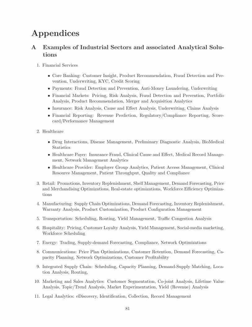
Appendices

A Examples of Industrial Sectors and associated Analytical Solu-tions

1. Financial Services

• Core Banking: Customer Insight, Product Recommendation, Fraud Detection and Pre-vention, Underwriting, KYC, Credit Scoring

• Payments: Fraud Detection and Prevention, Anti-Money Laundering, Underwriting

• Financial Markets: Pricing, Risk Analysis, Fraud Detection and Prevention, PortfolioAnalysis, Product Recommendation, Merger and Acquisition Analytics

• Insurance: Risk Analysis, Cause and Effect Analysis, Underwriting, Claims Analysis

• Financial Reporting: Revenue Prediction, Regulatory/Compliance Reporting, Score-card/Performance Management

2. Healthcare

• Drug Interactions, Disease Management, Preliminary Diagnostic Analysis, BioMedicalStatistics

• Healthcare Payer: Insurance Fraud, Clinical Cause and Effect, Medical Record Manage-ment, Network Management Analytics

• Healthcare Provider: Employer Group Analytics, Patient Access Management, ClinicalResource Management, Patient Throughput, Quality and Compliance

3. Retail: Promotions, Inventory Replenishment, Shelf Management, Demand Forecasting, Priceand Merchandising Optimizations, Real-estate optimizations, Workforce Efficiency Optimiza-tions

4. Manufacturing: Supply Chain Optimizations, Demand Forecasting, Inventory Replenishment,Warranty Analysis, Product Customization, Product Configuration Management

5. Transportation: Scheduling, Routing, Yield Management, Traffic Congestion Analysis

6. Hospitality: Pricing, Customer Loyalty Analysis, Yield Management, Social-media marketing,Workforce Scheduling

7. Energy: Trading, Supply-demand Forecasting, Compliance, Network Optimizations

8. Communications: Price Plan Optimizations, Customer Retention, Demand Forecasting, Ca-pacity Planning, Network Optimizations, Customer Profitability

9. Integrated Supply Chain: Scheduling, Capacity Planning, Demand-Supply Matching, Loca-tion Analysis, Routing,

10. Marketing and Sales Analytics: Customer Segmentation, Co-joint Analysis, Lifetime ValueAnalysis, Topic/Trend Analysis, Market Experimentation, Yield (Revenue) Analysis

11. Legal Analytics: eDiscovery, Identification, Collection, Record Management

81

12. Customer Analytics: Customer Retention/Attraction, Pricing Optimizations, Brand Man-agement, Customer Life Cycle Management, Customer-specific Content Specialization, CallCenter Voice Analytics

13. Life Sciences: Gene Pool Analysis, Drug Discovery, BioInformatics

14. Human Resources: Churn Analysis, Talent Management, Benefits Analysis, Workforce Place-ment Optimizations, Call Center Staffing,

15. Government: Fraud Detection, Crime Prevention Management, Revenue Optimizations, TaxCompliance and Recovery Strategies, Transportation Planning

16. eCommerce: Web Metrics, Web-page Visitor Analysis, Customizable Site Designs, CustomerRecommendations, Online Advertisements, Online Trend Analysis, BLOG Analysis

82