I Spatial Models in Population Biology

I Spatial Models in Population Biology

Jan M. Swart

Lecture 1: Interacting Particle Systems

Jan M. Swart Spatial Models in Population Biology

Interacting Particle Systems

Outline

I Poisson construction of continuous-time Markov chains

I Poisson construction of interacting particle systems

I Unique ergodicity

I Examples


Continuous-time Markov chains

Let S be a countable set. A probability kernel on S is a functionK : S2 → [0, 1] such that

∑y K (x , y) = 1. We calculate with

kernels as with matrices:

KL(x , z) :=∑y

K (x , y)L(y , z) and Kf (x) :=∑y

K (x , y)f (y).

Let X = (Xt)t≥0 be a stochastic process taking values in acountable set S . We assume that the sample paths of X arepiecewise constant and right-continuous. By definition, X is a(time-homogenous) Markov process if

P[Xu ∈ ·

∣∣ (Xs)0≤s≤t]

= Pu−t(Xt , · ) a.s. (0 ≤ t ≤ u),

where the transition kernels (Pt)t≥0 form a collection of probabilitykernels on S such

PsPt = Ps+t and limt↓0

Pt = P0 = 1.


Continuous-time Markov chains

We would like to define (Pt)t≥0 in terms of its generator

G (x , y) := limt↓0

t−1(Pt(x , y)− 1(x , y)

),

where 1(x , y) := 1x=y denotes the identity matrix. Such agenerator must satisfy

G (x , y) ≥ 0 (x 6= y) and∑y

G (x , y) = 0.

We interpret G (x , y) (x 6= y) as the rate of transitions x 7→ y . Weshould have

Px [Xt = y ] = Pt(x , y) = 1(x , y) + tG (x , y) + O(t2) as t ↓ 0,

where Px denotes the law of the process started in X0 = x .


Generator construction of continuous-time Markov chains

If S is finite, then we can define

Pt = e tG :=∞∑n=0

1

n!tnGn (t ≥ 0).

This works more generally if G is bounded in the sense that

supx

∑y : y 6=x

G (x , y) <∞.


Generator construction of continuous-time Markov chains

Let G be a Markov generator on a countable set S . Then, for eachz ∈ S , there exists a unique minimal solution to the backwardequations

∂∂t Pt(x , z) =

∑y

G (x , y)Pt(y , z) (t ≥ 0, x ∈ S).

Moreover, (Pt)t≥0 is a semigroup of subprobability kernels. Foreach initial state X0 = x ∈ S , there exists a process X = (Xt)t≥0

with values in S ∪ ∞ such that

Xt =∞ ∀t ≥ τ := inft ≥ 0 : Xt =∞,limt↑τ

Xt =∞ if τ <∞,

Px[Xu ∈ y

∣∣ (Xs)0≤s≤t]

= Pu−t(Xt , y) a.s. (y ∈ S , t ≤ u).

If Px [τ =∞] = 1 for all x ∈ S , then X is nonexplosive.


Example: a finite contact process

Let (Λ,E ) be a finite directed graph with vertex set Λ and set ofdirected edges E ⊂ Λ× Λ. Let S = 0, 1Λ be the space of allfunctions x : Λ→ 0, 1. We interpret x = (x(i))i∈Λ as a particleconfiguration where for i ∈ Λ,

x(i) = 0 means the site i is empty,

x(i) = 1 means there is a particle at i .

The contact process with infection rate λ ≥ 0 is a continuous-timeMarkov chain X = (Xt)t≥0 with state space S . In each jump, thenumber of occupied sites can increase or decrease by one. Letx ∈ S and j ∈ Λ such that x(j) = 0. Then

G (x , x + δj) := λ∑

(i ,j)∈E

x(i) and G (x + δj , x) := 1.

We set G (x , y) := 0 if x and y differ in more than one site andchoose G (x , x) such that

∑y G (x , y) = 0.



For each (i , j) ∈ E , define a branching map braij : S → S by

braijx(k) :=

x(i) ∨ x(j) if k = j ,

x(k) otherwise.

For each i ∈ Λ, define a death map deathi : S → S by

deathix(k) :=

0 if k = i ,

x(k) otherwise.

Fix x . Assume that Xt satisfies for all (i , j) ∈ E resp. i ∈ Λ,

Xt =

braijx with probability λt + O(t2),

deathix with probability t + O(t2),

x with probability 1− λt|E | − t|Λ|+ O(t2).

Then P[Xt = y ] = 1(x , y) + tG (x , y) + O(t2).


Poisson construction of continuous-time Markov chains

Idea: construct a continuous time Markov chain by applying mapsm : S → S at times of a Poisson process.

Let (Ω,F , µ) be a measurable space with σ-finite, nonatomicmeasure µ. Recall that a Poisson point set with intensity µ is arandom subset ω ⊂ Ω such that∣∣ω ∩ A

∣∣ is Poisson distributed with mean µ(A)

whenever A ∈ F , µ(A) <∞, and∣∣ω ∩ A1

∣∣, . . . , ∣∣ω ∩ An

∣∣ are independent

whenever A1, . . . ,An are disjoint. In particular, if ε := µ(A) issmall, then

P[|ω ∩ A

∣∣ = 1]

= ε+ O(ε2), P[|ω ∩ A

∣∣ ≥ 2]

= O(ε2).



Each generator G has a random mapping representation

G (x , y) =∑m∈G

rm(1m(x) = y − 1x = y

),

where (rm)m∈G are nonnegative rates and G is a collection of mapsm : S → S . Let ω be a Poisson point set on G × R with intensity

µ(m × A

)= rm `(A)

(A ∈ B(R)

),

where B(R) is the Borel-σ-field on R and ` denotes Lebesguemeasure. If

∑m∈G rm <∞, then we may order the elements of

ωs,t := ω ∩ G × (s, t] =

(m1, t1), . . . , (mn, tn)

with t1 < · · · < tn.



Define random maps Xs,t : S → S (s ≤ t) by

Xs,t := mn · · · m1.

(Poisson construction of Markov processes) Definemaps (Xs,t)s≤t as above in terms of a Poisson point setω. Let X0 be an S-valued random variable, independentof ω. Then

Xt := X0,t(X0) (t ≥ 0)

is a Markov process with generator G.

Remark The sample paths of X are right-continuous. We getleft-continuous paths by defining

Xs,t− in terms of ωs,t− := ω ∩ G × (s, t).



time

space

0 1 2 3 4 5 6 7 8 90 0 0 0 1 0 1 1 0 0

0 0 0 1 1 1 1 1 0 0

X0,t(x)

x

bra2,1

bra0,1

bra4,3bra7,8

bra2,3

death4

bra3,4bra1,2

bra6,5

bra7,6

death8


Stochastic flows

The random maps (Xs,t)s≤t form a stochastic flow

Xs,s = 1 and Xt,u Xs,t = Xs,u

with independent increments, in the sense that

Xt0,t1 , . . . ,Xtn−1,tn

are independent for each t0 < · · · < tn.

Different stochastic flows can define the same Markov process, asthere may be many different ways of writing down a randommapping representation

Gf (x) =∑m∈G

rm

f(m(x)

)− f(x),

for a given generator G .

Compare: Different SDE’s can define the same diffusion process.Jan M. Swart Spatial Models in Population Biology

Form of the generator

Here we have used that for any function f : S → R,

Gf (x) =∑y

G (x , y)f (y)

=∑y

∑m∈G

rm(1m(x) = y − 1x = y

)f (y)

=∑m∈G

rm

f(m(x)

)− f(x).

Then, as t ↓ 0,

Ex[f (Xt)

]= f (x) + tGf (x) + O(t2)

=(

1− t∑m∈G

rm)

f (x) + t∑m∈G

rmf(m(x)

)+ O(t2).


Example: the contact process

Let (Λ,E ) be a finite directed graph. The contact process on(Λ,E ) with infection rate λ ≥ 0 is the continuous-time Markovchain X = (Xt)t≥0 with state space 0, 1Λ and generator

Gf (x) :=λ∑

(i ,j)∈E

f(braijx

)− f (x)

+∑i∈Λ

f(deathix

)− f (x)

.

We would like to define contact processes on infinite lattices, e.g.,Λ = Zd with E = (i , j) : |i − j | = 1.If Λ is infinite, then we equip 0, 1Λ with the product topologywhich corresponds to pointwise convergence

xn → x iff xn(i)→ x(i) ∀i ∈ Λ.

By Tychonoff’s theorem, 0, 1Λ is a compact space.


Feller processes

Let S be a compact metrizable space. Let C(S) denote the spaceof all continuous functions f : S → R, equipped with thesupremumnorm ‖ · ‖∞, and let M1(S) denote the space of allprobability measures on S , equipped with the topology of weakconvergence.For any probability kernel K (x , dy) on S and measurable functionf : S → R, we define

Kf (x) :=

∫S

K (x ,dy)f (y) (x ∈ S).

By definition, a Feller semigroup is a collection of probabilitykernels (Pt)t≥0 on S such that:

(i) P0 = 1 and PsPt = Ps+t (s, t ≥ 0),

(ii) S × [0,∞) 3 (x , s) 7→ Ps(x , · ) ∈M1(S) is continuous.


Feller processes

The generator of a Feller semigroup is the operator G defined as

Gf := limt↓0

t−1(Pt f − f ) (∗),

with domain

D(G ) :=

f ∈ C(S) : the limit in (∗) exists in the norm ‖ · ‖∞.

The Hille-Yosida theorem gives necessary and sufficient conditionsfor an operator G to generate a Feller semigroup.

The domain D(G ) is a dense subspace of C(S). For eachf ∈ D(G ), the function t 7→ Pt f is given by the unique solution tothe backward equation

∂∂t Pt f = GPt f (t ≥ 0) with P0f = 1.


Feller processes

Let S be a compact metrizable space and let (Pt)t≥0 be a Fellersemigroup of transition kernels on S .Then, for each probability law µ on S , there exists a process(Xt)t≥0 such that

I The sample paths t 7→ Xt are a.s. cadlag, i.e.,right-continuous with left limits.

I P[X0 ∈ · ] = µ.

I Px[Xu ∈ ·

∣∣ (Xs)0≤s≤t]

= Pu−t(Xt , · ) a.s. (t ≤ u).

Such a process is called a Feller process.


Poisson construction of Interacting Particle Systems

For any map m : SΛ → SΛ, let

D(m) :=

i ∈ Λ : ∃x ∈ SΛ s.t. m(x)(i) 6= x(i)

denote the set of lattice points whose values can possibly bechanged by m. By definition, m is a local map if and only if

(i) D(m) is finite,

(ii) m is continuous w.r.t. the product topology.

Say that a site j ∈ Λ is m-relevant for some i ∈ Λ if

∃x , y ∈ SΛ s.t. m(x)(i) 6= m(y)(i) and x(k) = y(k) ∀k 6= j ,

and define

Ri (m) :=

j ∈ Λ : j is m-relevant for i.



Remark A map m : SΛ → SΛ is continuous w.r.t. the producttopology if and only if for each i ∈ Λ:

(i) Ri (m) is finite,

(ii) x(j) = y(j) for all j ∈ Ri (m) implies m(x)(i) = m(y)(i).

TriviallyRi (m) = i if i 6∈ D(m).

In our example:

D(braij) = j Rj(braij) = i , j,D(deathi ) = i Ri (deathi ) = ∅.



Let G me a collection of local maps m : SΛ → SΛ and let (rm)m∈Gbe nonnegative constants. As before, we let ω be a Poisson pointset on G × R with intensity

µ(m × A

)= rm `(A)

(A ∈ B(R)

).

For infinite lattices (e.g., for the contact process on Zd) wetypically have

∑m∈G rm =∞ which means

ωs,t := ω ∩ G × (s, t]

has a.s. infinitely many elements for any s < t. As a result, wecannot order the elements of ωs,t by their time coordinates.Nevertheless, for each finite subset ω ⊂ ωs,t , we can still define

Xωs,t(x) := mn · · · m1(x) (x ∈ SΛ, s ≤ t),

where ω = (m1, t1), . . . , (mn, tn) with t1 < · · · < tn.



Theorem Assume that

supi∈Λ

∑m∈GD(m)3i

rm|Ri (m)| <∞.

Then a.s., for each x ∈ SΛ the limit

Xs,t(x) := limωn↑ωs,t

Xωns,t(x)

exists, does not depend on the sequence of finite sets ωn ↑ ωs,t ,and defines a stochastic flow (Xs,t)s≤t . If X0 is an SΛ-valuedrandom variable, independent of ω, then

Xt := X0,t(X0) (t ≥ 0)

defines a Feller process with generator

Gf (x) =∑m∈G

rm

f(m(x)

)− f(x).



Lemma 1 One has

E[∣∣Ri (Xs,t)

∣∣] ≤ eR(t − s) (s ≤ t),

whereR := sup

i∈Λ

∑m∈GD(m)3i

rm(|Ri (m)| − 1

). (1)



time

space

0 1 2 3 4 5 6 7 8 90 0 0 0 1 0 1 1 0 0

X0,t(4)

x

bra2,1

bra2,1

bra0,1

bra4,3

bra4,3

bra7,8

bra2,3

bra2,3

death4

death4

bra3,4

bra3,4

bra1,2

bra6,5

bra7,6

death8



time

space

0 1 2 3 4 5 6 7 8 90 0 0 0 1 0 1 1 0 0

X0,t(4)

x

bra2,1

bra2,1

bra0,1

bra4,3

bra4,3

bra7,8

bra2,3

bra2,3

death4

death4

bra3,4

bra3,4bra1,2

bra6,5

bra7,6

death8



time

space

0 1 2 3 4 5 6 7 8 90 0 0 0 1 0 1 1 0 0

X0,t(4)

x

bra2,1

bra2,1

bra0,1

bra4,3

bra4,3bra7,8

bra2,3

bra2,3

death4

death4

bra3,4

bra3,4bra1,2

bra6,5

bra7,6

death8



time

space

0 1 2 3 4 5 6 7 8 90 0 0 0 1 0 1 1 0 0

X0,t(4)

x

bra2,1bra2,1

bra0,1

bra4,3bra4,3bra7,8

bra2,3bra2,3

death4death4

bra3,4bra3,4bra1,2

bra6,5

bra7,6

death8


Generator construction of Interacting Particle Systems

For any f ∈ C(SΛ) and i ∈ Λ, we define

δf (i) := sup|f (x)− f (y)| : x , y ∈ SΛ, x(j) = y(j) ∀j 6= i

,

Csum :=

f ∈ C(SΛ) : ‖‖f ‖‖ :=∑i∈Λ

δf (i) <∞

We call f ∈ Csum a function of summable variation. One has∣∣f (x)− f (y)∣∣ ≤ ∑

i : x(i) 6=y(i)

δf (i) ≤ ‖‖f ‖‖.

Lemma 2 If (Pt)t≥0 is the Feller semigroup of an interactingparticle system with generator G , then Csumm ⊂ D(G ) and

‖‖Pt f ‖‖ ≤ eRt‖‖f ‖‖ (t ≥ 0),

where R is the constant in (1).


Generator construction of Interacting Particle Systems

For any probability kernel κ on SΛ, set

D(κ) :=

i ∈ Λ : ∃x s.t. κ(x , y : y(i) 6= x(i)

)> 0.

By definition, a local probability kernel is a probab. kernel suchthat

(i) D(κ) is finite,(ii) x 7→ κ(x , · ) is continuous w.r.t. weak convergence.

Liggett (1985) writes generators in the form

Gf (x) =∑κ∈K

rκ∫

κ(x , dy) f (y)− f (x),

where K is a collection of local probability kernels and (rκ)κ∈K arenonnegative rates. Under suitable conditions on the rates, heproves the closure of G generates a Feller semigroup and

‖‖Pt f ‖‖ ≤ eR ′t‖‖f ‖‖ (t ≥ 0)

for some constant R ′ <∞.Jan M. Swart Spatial Models in Population Biology

Proofs

Proof of Lemma 1 By a cut-off argument, w.l.o.g. we assumethat Λ is finite. Then we can apply our previous result about thePoisson construction of continuous-time Markov chains toconclude that (

Ri (X−t,0))t≥0

is a set-valued Markov process that can be bounded from above bya process that jumps as

A 7→ (A\D(m)) ∪⋃

i∈D(m)∩A

Ri (m) with rate rm

for each m ∈ G. Let (Pt)t≥0 denote the semigroup of theset-valued process and let G be its generator. Let f be thefunction f (A) := |A|. Then

Gf (A) =∑m∈G

rm

f((A\D(m)) ∪

⋃i∈D(m)∩A

Ri (m))− f (A)


Proofs

It follows that

Gf (A)≤∑m∈G

rm∑

i∈D(m)∩A

(|Ri (m)| − 1

)=∑i∈A

∑m:D(m)3i

rm(|Ri (m)| − 1

)≤ R|A|,

and hence

∂∂t

(e−RtPt f

)= −Re−RtPt f +e−RtPtGnf = e−RtPt(Gnf −Rf ) ≤ 0

and therefore e−RtPt f ≤ e−R0P0f = f , which means in particularthat

E[|Ri (X−t,0)|

]= Pt f (i) ≤ eRt f (i) = eRt (t ≥ 0).


Proofs

Proof of Lemma 2 We want to prove that

‖‖Pt f ‖‖ ≤ eRt‖‖f ‖‖ with ‖‖f ‖‖ :=∑i∈Λ

δf (i).

Fix i ∈ Λ and let x , y ∈ SΛ with x(j) = y(j) ∀j 6= i . Then∣∣Pt f (x)− Pt f (y)| =∣∣E[f (X0,t(x))]− E[f (X0,t(y))]

∣∣≤ E

[∣∣f (X0,t(x))− f (X0,t(y))∣∣]

≤∑j

P[X0,t(x)(j) 6= X0,t(y)(j)

]δf (j)

≤∑j

P[i ∈ Rj(X0,t)

]δf (j)

It follows that∑i

δPt f (i) ≤∑ij

P[i ∈ Rj(X0,t)

]δf (j) ≤ eRt

∑j

δf (j).


Unique ergodicity

For any probability measure µ on SΛ, write

µPt :=

∫µ(dx)Pt(x , · ) (t ≥ 0).

If X = (Xt)t≥0 has initial law P[X0 ∈ · ] = µ, then,

P[Xt ∈ A] =

∫P[X0 ∈ dx ]P[Xt ∈ A |X0 ∈ dx ] =

∫µ(dx)Pt(x ,A),

i.e., Xt has law µPt .By definition, a probability measure ν on SΛ is an invariant law if

νPt = ν (t ≥ 0).

The process X = (Xt)t≥0 is stationary if and only if P[X0 ∈ · ] isan invariant law.


Unique ergodicity

Proposition If the constant R from (1) satisfies R < 0, then theinteracting particle system has a unique invariant law ν, and

µPt =⇒t→∞

ν

for any initial law µ.

Proof If R < 0, then

P[Ri (X0,t) = ∅

]−→t→∞

1.

As a consequence, the limit

Xt(i) := lims→∞

Xt−s,t(x)(i) (i ∈ Λ)

exists a.s. for each i ∈ Λ and t ∈ R, and does not depend on thechoice of x ∈ SΛ.


Unique ergodicity

One can check that this defines a stationary process (Xt)t∈R. LetY have law µ and be independent of the Poisson processes used toconstruct the flow (Xs,t)s≤t . Then X−t,0(Y ) has law µPt and

X−t,0(Y ) −→t→∞

X0 a.s.,

proving that µPt =⇒t→∞

ν.

Remark 1 This method is called coupling from the past.

Remark 2 The proof works more generally if

P[Ri (X0,t) = ∅

]−→t→∞

1 (i ∈ Λ),

which may happen even if R ≥ 0.


The contact process

Recall that

D(braij) = j Rj(braij) = i , j,D(deathi ) = i Ri (deathi ) = ∅.

For the nearest neighbor contact process on Zd , this yields

R = 2dλ− 1,

which is < 0 iff λ < 1/2d . Since Xs,t(0) = 0, we conclude that forλ < 1/2d , the measure δ0 is the unique invariant law.


The contact process

Contact process with infection rate λ = 2 and death rate d = 1.Time t = 0.


The contact process



A stochastic Ising model

Let (Λ,E ) be an undirected graph and let S = −1,+1. For anyx ∈ SΛ, we call

Mi (x) :=∑

j : i ,j∈E

x(j)

the local magnetization around i ∈ Λ. Let κi (x , · ) denote the lawof a random variable X such that

P[X (i) = ±1] =eβ±Mi (x)

eβ±Mi (x) + eβ∓Mi (x),

and X (j) = x(j) a.s. for all j 6= i . Then κi is a local probabilitykernel and

Gf (x) =∑i∈Λ

( ∫κi (x , dy)f (y)− f (x)

)defines the generator of a stochastic Ising model with Glauberdynamics.


A stochastic Ising model

When the parameter β is large, nearby spins like have the samesign.We start the process in product measure for different values of βand see what happens.


The Ising model

β = 0.3, time t = 0.


The Ising model

β = 0.3, time t = 1.


The Ising model

β = 0.3, time t = 2.


The Ising model

β = 0.3, time t = 4.


The Ising model

β = 0.3, time t = 8.


The Ising model

β = 0.3, time t = 16.


The Ising model

β = 0.3, time t = 32.


The Ising model

β = 0.3, time t = 64.


The Ising model

β = 0.7, time t = 0.


The Ising model

β = 0.7, time t = 1.


The Ising model

β = 0.7, time t = 2.


The Ising model

β = 0.7, time t = 4.


The Ising model

β = 0.7, time t = 8.


The Ising model

β = 0.7, time t = 16.


The Ising model

β = 0.7, time t = 32.


The Ising model

β = 0.7, time t = 64.


The Ising model

β = 0.7, time t = 125.


The Ising model

β = 0.7, time t = 250.


The Ising model

β = 1, time t = 0.


The Ising model

β = 1, time t = 1.


The Ising model

β = 1, time t = 2.


The Ising model

β = 1, time t = 4.


The Ising model

β = 1, time t = 8.


The Ising model

β = 1, time t = 16.


The Ising model

β = 1, time t = 32.


The Ising model

β = 1, time t = 64.


The Ising model

β = 1, time t = 125.


The Ising model

β = 1, time t = 250.


The Ising model

β = 1, time t = 500.


A stochastic Potts model

Instead of allowing only two states −1,+1, we can more generallyallow q ≥ 2 states 1, . . . , q.Each person i chooses a new state at times of a Poisson processwith rate 1.The probability that the newly chosen state is k ∈ 1, . . . , qequals

eβMi (k)∑qm=1 eβMi (m)

,

where Mi (k) denotes the number of neighbors of i that are in thestate k .Setting q = 2 and replacing β by 2β yields the Ising model.


The Potts model

β = 1.2, time t = 0.


The Potts model

β = 1.2, time t = 1.


The Potts model

β = 1.2, time t = 2.


The Potts model

β = 1.2, time t = 4.


The Potts model

β = 1.2, time t = 8.


The Potts model

β = 1.2, time t = 16.


The Potts model

β = 1.2, time t = 32.


The Potts model

β = 1.2, time t = 64.


The Potts model

β = 1.2, time t = 125.


The Potts model

β = 1.2, time t = 250.


The Potts model

β = 1.2, time t = 500.


The voter model

In the voter model, each site i ∈ Λ is occupied by an organism withgenetic type x(i) ∈ S .

The organism at site i dies at times of a Poisson process with rate1 and is replaced by the offspring of a randomly chosen neighbor.

Using the voter map

votji (x)(k) :=

x(j) if k = i ,x(k) otherwise,

we can give the following random mapping representation of thegenerator:

Gf (x) =∑

(i ,j)∈E

1

Ni

f(votjix

)− f(x),

where Ni :=∣∣j : (j , i) ∈ E

∣∣ is the number of neigbors of i .


The voter model

Time t = 0.


The voter model

Time t = 0.25.


The voter model

Time t = 0.5.


The voter model

Time t = 1.


The voter model

Time t = 2.


The voter model

Time t = 4.


The voter model

Time t = 8.


The voter model

Time t = 16.


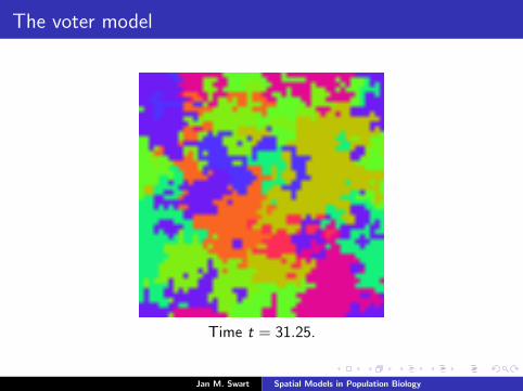
The voter model

Time t = 31.25.


The voter model

Time t = 62.5.


The voter model

Time t = 125.


The voter model

Time t = 250.


The voter model

Time t = 500.


The voter model

The behavior of the voter model strongly depends on thedimension.

Clustering in dimensions d = 1, 2.

Stable behavior in dimensions d ≥ 3.


The voter model

Cut of 3-dimensional model, time t = 0.


The voter model



A one-dimensional voter model

space

time

0 100 200 300 400 500

0

500

1000

1500

2000

2500

A one-dimensional voter model.


A one-dimensional Potts model

space

time

0 100 200 300 400 500

0

500

1000

1500

2000

2500

In one-dimensional Potts models, the cluster size remainsbounded in time even at very high β (= low temperature).


The biased voter model

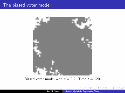
In the biased voter model with two states 0, 1, each organism ichanges its type Xt(i) with the rates

0 7→ 1 with rate (1 + s) · fraction of type 1 neighbors,

1 7→ 0 with rate 1 · fraction of type 0 neighbors,

where s > 0 gives type 1 a (small) advantage.

Contrary to the voter model, even if we start with just a singleorganism of type 1, there is a positive probability that type 1 neverdies out.

Models spread of advantageous mutation.



Biased voter model with s = 0.2. Time t = 0 .



Biased voter model with s = 0.2. Time t = 10.



space

time

0 100 200 300 400 500

0

100

200

300

400

A one-dimensional biased voter model with bias s = 0.2.



We can extend the biased voter model by also allowingspontaneous jumps from 1 to 0.

0 7→ 1 with rate (1 + s) · fraction of type 1 neighbors,

1 7→ 0 with rate 1 · fraction of type 0 neighbors

+ d ,

where s > 0 gives type 1 an advantage and d ≥ 0 is a death rate.

This models the fact that genes may become disfunctional due todeleterious mutations.

Whether 1’s have a positive probability to survive now depends ina nontrivial way on s and d .



space

time

0 100 200 300 400 500

0

200

400

600

Process with bias s = 0.5, death rate d = 0.02.


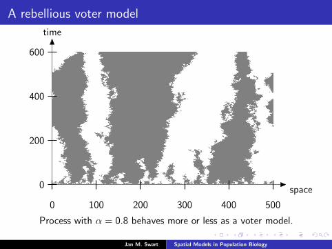
A rebellious voter model

The rebellious voter map is defined as

rvotkji (x)(l) :=

1− x(i) if l = i and x(k) 6= x(j),

x(l) otherwise.

The rebellious voter model is the one-dimensional model withgenerator

Gf (x) :=α∑i

f(voti ,i+1(x)

)− f(x)

+α∑i

f(voti ,i−1(x)

)− f(x)

+(1− α)∑i

f(rvoti−1,i ,i+1(x)

)− f(x)

+(1− α)∑i

f(rvoti+1,i ,i−1(x)

)− f(x).



space

time

0 100 200 300 400 500

0

200

400

600

Process with α = 0.8 behaves more or less as a voter model.



space

time

0 100 200 300 400 500

0

200

400

600

In the process with α = 0.3, cluster size remains bounded in time.


Reaction diffusion models

Another rich class of models are reaction diffusion models.

These are systems of particles that perform independent randomwalks and interact when they are near to each other.

Let Xt(i) = 1 (resp. 0) signify the presence (resp. absence) of aparticle and consider the maps rwij : 0, 1Z → 0, 1Z

rwi ,jx(k) :=

0 if k = i ,

x(i) ∨ x(j) if k = j ,x(k) otherwise.

The process with generator

G = 12

∑i∈Z

f(rwi ,i+1x

)− f(x)

+ 12

∑i∈Z

f(rwi ,i−1x

)− f(x)

describes coalescing random walks.


Coalescing random walks

space

time

0 50 100 150 200

0

100

200

300

400


Reaction diffusion models

In analogy with the branching map

braijx(k) :=

x(i) ∨ x(j) if k = j ,

x(k) otherwise,

we can also define a cooperative branching map

coopii ′jx(k) :=

(x(i) ∧ x(i ′)

)∨ x(j) if k = j ,

x(k) otherwise.


Branching and coalescing random walks

space

time

0 50 100 150 200

0

100

200

300

400


Cooperative branching and coalescence

space

time

0 50 100 150 200

0

100

200

300

400

Cooperative branching rate 2.2.


Cooperative branching

space

time

0 50 100 150 200

0

100

200

300

400

Cooperative branching rate 3.


A cancellative system

Two more maps of interest are the annihilating random walk map

arwijx(k) :=

0 if k = i ,

x(i) + x(j) mod(2) if k = j ,x(k) otherwise,

and the annihilating branching map

abraijx(k) :=

x(i) + x(j) mod(2) if k = j ,

x(k) otherwise,



space

time

0 50 100 150 200

0

100

200

300

400

Annihilating random walks.



space

time

0 50 100 150 200

0

10

20

30

40

A system of branching annihilating random walks.


Killing

Define a killing map as

killijx(k) :=

(1− x(i)

)∧ x(j) if k = j ,

x(k) otherwise,

which says that the particle at i , if present, kills any particle at j .


Branching and killing

space

time

0 50 100 150 200

0

100

200

300

400

A system with branching and killing.


I Spatial Models in Population Biology

Documents

Transcript of I Spatial Models in Population Biology