I L R E Robust Estimation and B Inference for Threshold...

SFB 649 Discussion Paper 2013-034

Robust Estimation and

Inference for Threshold Models with Integrated Regressors

Haiqiang Chen*

* Xiamen University, China

This research was supported by the Deutsche Forschungsgemeinschaft through the SFB 649 "Economic Risk".

http://sfb649.wiwi.hu-berlin.de

ISSN 1860-5664

SFB 649, Humboldt-Universität zu Berlin Spandauer Straße 1, D-10178 Berlin

SFB

6

4 9

E

C O

N O

M I

C

R I

S K

B

E R

L I

N

Robust Estimation and Inference for Threshold Models with

Integrated Regressors

Haiqiang Chen�

Wang Yanan Institute for Studies in Economics, MOE Key Laboratory of Econometrics,and Fujian Key Laboratory of Statistical Science, Xiamen University, Fujian 361005, China

July 1, 2013

Abstract

This paper studies the robust estimation and inference of threshold models with integrated regres-

sors. We derive the asymptotic distribution of the pro�led least squares (LS) estimator under the

diminishing threshold e¤ect assumption that the size of the threshold e¤ect converges to zero. Depend-

ing on how rapidly this sequence converges, the model may be identi�ed or only weakly identi�ed and

asymptotic theorems are developed for both cases. As the convergence rate is unknown in practice, a

model-selection procedure is applied to determine the model identi�cation strength and to construct

robust con�dence intervals, which have the correct asymptotic size irrespective of the magnitude of

the threshold e¤ect. The model is then generalized to incorporate endogeneity and serial correlation

in error terms, under which, we design a Cochrane-Orcutt feasible generalized least squares (FGLS)

estimator which enjoys e¢ ciency gains and robustness against di¤erent error speci�cations, including

both I(0) and I(1) errors. Based on this FGLS estimator, we further develop a sup-Wald statistic to

test for the existence of the threshold e¤ect. Monte Carlo simulations show that our estimators and

test statistics perform well.

JEL Classi�cation: C12, C22, C52

Keywords: Threshold e¤ects; Integrated processes; Nonlinear cointegration; Weak identi�cation.

�E-mail: [email protected]. I would like to thank Yongmiao Hong, Jiti Gao, Wolfgang Härdle, Zongwu Cai, YingFang, Nicholas M. Kiefer, George H. Jakubson and seminar participants at Cornell University and the 3rd XMU-HumboldtWorkshop on �Nonparametric and Nonstationary Econometrics� for helpful comments. I acknowledged the �nancialsupport from the Chinese National Science Foundation Grant 11201390, 71201137, 71131108 and 71271179. The researchwas also partially supported by Deutsche Forschungsgemeinschaft (DFG) through the SFB649 �Economic Risk�. Allremaining errors are mine.

1

1 Introduction

Threshold models, in which the model parameters switch when the value of a certain variable crosses

a threshold, have received much attention over the past two decades. Given their ability to capture a

very rich set of stylized facts of modern economics, such as multiple states, asymmetries and cyclical

e¤ects, the use of threshold models has been advocated in many empirical applications. Examples

include the analysis of asymmetries in persistence in US output growth (Potter, 1995), nonlinearities in

unemployment rates (Hansen, 1997), and multiple states in cross-country growth regressions (Durlauf

and Johnson, 1995, Hansen, 2000), among numerous others. The estimation and asymptotics for

variants of threshold models have been well established by Chan (1993), Hansen (1996, 2000), Tsay

(1998), Gonzalo and Pitarakis (2002), and Seo and Linton (2007) etc.. More recently, Yu (2012)

studies likelihood-based estimation and inference for a parametric discontinuous threshold regression

model while Li and Ling (2012) study the least squares (LS) estimator of the multiple-regime threshold

autoregressive (TAR) model.

However, most of the aforementioned studies maintain a restrictive assumption that the data should

be either i.i.d. or stationary processes. Two exceptions are Caner and Hansen (2001) who study

a threshold autoregressive model with a unit root and Gonzalo and Pitarakis (2006) who design a

Wald statistic to test the threshold e¤ect in a cointegrating regression. To the best of our knowledge,

the asymptotic properties of threshold estimators, when all or some of the regressors are integrated

processes, have not been established. In this paper, we investigate the robust estimation of threshold

models with integrated regressors and establish its asymptotic properties allowing for di¤erent model

identi�cation strengths, endogenous regressors and serially correlated error terms, including both I(0)

and I(1) errors.

Speci�cally, we consider a threshold model of the following form:

yt =

(�01xt + ut; if qt � 0�02xt + ut; if qt > 0

, (1)

where xt is a d1-dimensional vector of integrated process of order 1 (I(1)) and yt is the dependent

variable.1 The error term, which will be speci�ed more precisely later, is denoted by ut; and qt is the

threshold variable. The threshold value 0 2 [ ; ] is an unknown parameter pending estimation. Ifut is a stationary process, Equation (1) can be regarded as a special case of nonlinear cointegration

models,2 see Karlsen et al. (2007), Wang and Phillips (2009), Gao et al. (2009a, 2009b), Bierens and

Martins (2010) and Choi and Saikkonen (2010).

Equation (1) can be rewritten as

yt = �0xt + �

0xtI(qt � 0) + ut; (2)

1The model could be to extended to include an intercept term and stationary regressors.2Loosely speaking, if the response variable yt is generated by a nonlinear transformation of integrated regressors xt

plus a stationary error term, then there exists a nonlinear cointegrating relationship between yt and xt:

2

where � = �2 and � = �1 � �2: Here I(qt � 0) is an indicator function taking the value one if

qt � 0 and zero otherwise. The vector (1;��) can be regarded as a benchmark long-run relationshipbetween yt and xt and the term �xtI(qt � 0) captures the deviation from the linear equilibrium. In

the literature, � is often assumed to be a deterministic sequence converging to zero at some rate as the

sample size n increases. This assumption is not only convenient for deriving the asymptotic distribution

of threshold estimators as in Hansen (2000), but is also relevant in many empirical applications. For

example, an important issue in the empirical �nance literature is to investigate whether fundamental

variables, such as the dividend-price ratio and the earning-price ratio, can predict asset returns. Linear

prediction models have been extensively studied, but have failed to generate any unanimous conclusion

(for more detail, refer to Campbell and Yogo, 2006).3 Recently, Gonzalo and Pitarakis (2012) document

a regime-speci�c predictability of S&P 500 index returns from the dividend ratio based on a threshold

model. However, as is well known, stock returns commonly behave as martingale di¤erences, while

fundamental variables are highly persistent (integrated or nearly integrated processes). This imbalance

on the order of integration implies that such predictive relationship should be very weak, which happens

if and only if � = 0 and � is around zero in Equation (2).

In this paper, we follow the literature by assuming the size of threshold e¤ect converges to zero.

Depending on how rapidly this sequence converges, the threshold value 0 may be identi�ed or only

weakly identi�ed and we develop asymptotic theorems for both cases.4 In the �rst case, we show that the

pro�led LS estimator is consistent and that its con�dence intervals (CIs) can be constructed through

inversion of certain standard test statistics; whereas in the second case, the pro�led LS estimator

is inconsistent and its limiting distribution depends on some inestimable nuisance parameters. The

standard method to construct CIs does not control the coverage probability. We take the supremum

of quantiles for all possible values of nuisance parameters and then construct the least favorable CIs.

These CIs have the correct asymptotic size under the weak identi�cation case, but can be unnecessarily

long when the model is identi�ed. Motivated by Cheng (2008) and Shi and Phillips (2012), we then

propose a model-selection procedure to choose the CIs. It can be shown that the CIs chosen by this

method have approximately correct coverage probability irrespective of the magnitude of the threshold

e¤ect.

Furthermore, in a generalized model, we consider endogeneity and serial correlation, which are

common in empirical studies with integrated regressors. Following Saikkonen (1991), we assume the

error term to be an autoregressive (AR) process, and use leads and lags of innovations as extra re-

gressors to deal with endogeneity. We then design a Cochrane-Orcutt feasible generalized least squares

(FGLS) estimator to estimate the model. It is well known that, in linear cointegration models, the

FGLS estimator cannot improve the estimation e¢ ciency, as Phillips and Park (1988) demonstrate by

establishing their asymptotic equivalence. However, this equivalence does not hold when there exists

3Marmer (2008) shows that linear regression techniques actually may lead to spurious forecasts if there exist smalldepartures from the linear structure, but improvements of the forecast accuracy are possible if the nonlinear componentsare properly considered.

4See Elliott and Müller (2007) and Caner (2007) for weak identi�cation in break-point models; Cheng (2008) and Shiand Phillips (2012) for weak identi�cation in general nonlinear models.

3

a threshold e¤ect and we analytically and numerically show that the FGLS estimation achieves more

e¢ ciency compared to the pro�led LS estimation. The method to construct the robust CIs of the LS

estimator can also be generalized for the FGLS estimator.

Another attraction of the FGLS estimator is its robustness with respect to di¤erent error speci�ca-

tions, including both I(0) and I(1) errors. This robustness allows us to design a sup-Wald statistic to

test for the existence of threshold e¤ects without any requirement on the stationarity of the regression

error term and thus avoid the so-called joint hypothesis test problem in such models (see Balke and

Fomby, 1997). The idea is similar to Perron and Yabu (2009), who consider testing for structural

changes in the trend function of a time series using a quasi-FGLS procedure, without any requirement

on whether the noise component is stationary or integrated. In our case, we use the sup-Wald test

statistic based on the FGLS estimator to test for the existence of a threshold e¤ect and the critical

values are generated from a bootstrap method. Monte Carlo simulations show that the FGLS estimator

and the test statistic perform very well, even the error is an I(1) process.

The remainder of the paper is organized as follows. Section 2 presents the basic model. Section 3

considers the estimator and its asymptotics for the basic model. Section 4 generalizes the basic model

to allow for serially correlated errors and model endogeneity. Monte Carlo simulations are discussed in

Section 5. Section 6 concludes the paper. All proofs are in the appendices.

Throughout the paper, [ns] denotes the integer part of ns: The symbol �p!�represents convergence

in probability, �=)� represents weak convergence, and a:s:! represents almost sure convergence. All

limits are de�ned as the sample size n!1 unless otherwise stated. For a vector x; jj � jj signi�es theEuclidean norm, i.e., jjxjj =

Px2i : For a matrix A; jAj = (tr(A0A))1=2 denotes the Euclidean norm and

A0 denotes its transpose.Rdenotes integration from 0 to 1.

2 The Basic Model

The basic model we consider in the paper is given by

yt =

(�01xt + ut; if qt � 0�02xt + ut; if qt > 0

,

where xt is a d1-dimensional vector of unit root processes whose generating mechanism is given by

xt = xt�1 + vt; t = 1; 2; :::n

and we set x0 = 0 for convenience, although x0 = oa:s:(pn) is su¢ cient for the asymptotic results.

For the component time series ut and vt; we de�ne the following partial sums as

Un(s) �1pn

[ns]Xt=1

ut; and Vn(s) �1pn

[ns]Xt=1

vt: (3)

Before going further, we make the following assumptions.

4

(A1) sups2[0;1] jj(Un(s); Vn(s)) � (Bu(s);Bv(s))jja:s:! 0 as n ! 1; where (Bu(s);Bv(s)) is a vector

of Brownian motions with a positive de�nite long-run covariance matrix.

(A2) The error term ut satis�es: i) E(ut) = 0; Ejutj4 < 1; ii) For each n; there exists a �ltrationzn;t; t = 1; :::; n; such that f(ut;zn;t) : t � 1g is a stationary and ergodic martingale di¤erence sequencewith E(u2t jzn;t�1) = �2u < 1 almost surely for all t = 1; :::; n; iii) The term (qt; xt) is adapted to the

�ltration zn;t�1; t = 1; :::; n:(A3) i) The threshold parameter 0 2 [ ; ]; ii) The threshold variable qt is strictly stationary,

ergodic and ��mixing with mixing coe¢ cients �m satisfyingP1m=1 �

12� 1r

m < 1 for r > 2; iii) qt has a

continuous distribution F (�) and f(�) is the corresponding density function satisfying 0 < f( ) � f <1for all 2 [ ; ]:

(A4) The d1 dimensional I(1) vector xt is not cointegrated.

Assumption (A1) considers a strong approximation for (Un(s); Vn(s)); which is needed to derive the

convergence rate of the threshold estimator. This assumption is stronger than the weak convergence

result established by the multivariate invariance principle, but it is quite common in the literature,

see Park and Phillips (2001), Kasparis (2008), Wang and Phillips (2009a, 2009b) and Shi and Phillips

(2012), among others. Su¢ cient conditions to derive the strong approximation are also well developed

in the literature. For example, Park and Hahn (1999) establish conditions of strong approximations

for general linear processes. Shao and Lu (1987) and Cai et al. (2009) provide conditions of strong

approximations for an ��mixing process.Assumption (A2) supposes f(ut;zn;t) : t � 1g to be a martingale di¤erence sequence and (qt; xt) is

adapted to the �ltration zn;t�1; t = 1; :::; n. Under this assumption, qt and xt become predeterminedgiven the �ltration zn;t�1: One natural example of zt is the ��eld generated by the informationset f(ui; qi+1; xi+1) : 1 � i � tg. This assumption might be restrictive in linear cointegration models,but it is common in fully speci�ed cointegrating regression models. It allows for arguments based on

the martingale central limit theory to establish a weak convergence result for the empirical processP[ns]t=1 It(qt � )ut as in Caner and Hansen (2001).5 Assumption (A2) does not allow for serially

correlated errors and model endogeneity. However, in Section 4, we relax this assumption by adopting

the so-called �leads and lags�approach or dynamic OLS estimator proposed by Saikkonen (1991).

(A3) is very conventional in the literature of threshold models. The threshold variable qt is assumed

to be strictly stationary and strong mixing for asymptotic purposes. The assumption excludes the

case where qt is a unit root process, under which one may need to use another technique such as

the triangular array asymptotics proposed by Andrews and McDermott (1995). Assumption (A4) is

standard in the literature of regressions with integrated processes.

Following Caner and Hansen (2001), we de�ne W (s; �) as a two-parameter Brownian motion on

5The assumption (A2) can be relaxed under certain circumstances. For instance, ut could be generalized to follow alinear moving average process of �nite order l: However, fully generalizing the model to allow for serially correlated errorswould involve substantial added complexity (see Gonzalo and Pitarakis, 2006).

5

(s; �) 2 [0; 1]2, which is a zero-mean Gaussian process with covariance given by

E(W (s1; �1)W (s2; �2)) = (s1 ^ s2)(�1 ^ �2):

The two-parameter Brownian motion is a special tool to derive the limiting distribution in threshold

models with integrated processes. Note that when � = 1; we haveW (s; 1) �W (s), which is a Brownianmotion on s 2 [0; 1].

Moreover, we can de�ne the following stochastic integration with respect to W (s; �) on the �rst

argument (s) while holding the second argument (�) constant as

J1(�) =

ZBv(s)dW (s; �) = lim

n!1

nXt=1

(Bv(t� 1n)

�W (

t

n; �)�W ( t� 1

n; �)

�; (4)

where J1(�) is a Gaussian process with an almost surely continuous sample path and the covariance

kernel

E(J1(�1)J1(�2)) = (�1 ^ �2)ZBv(s)B

0v(s)ds:

3 Main Results

3.1 Pro�led LS Estimation and Asymptotics

For ease of manipulation, we rewrite Equation (2) in a more compacted form:

yt = �0At( 0) + ut; (5)

where At( 0) = (x0t; x

0t( 0))

0; xt( 0) = xtI(qt � 0); and � = (�0; �0)0.For any �xed 2 [ ; ]; the following model is estimated:

yt = b�( )0At( ) + but( );where b�( ) is given by

b�( ) = " nXt=1

At( )At( )0

#�1 " nXt=1

At( )yt

#:

The sum of squared residuals is de�ned as

SSRn( ) =

nXt=1

but( )2 = nXt=1

�yt � b�( )0At( )�2 ; (6)

and we de�ne the pro�led LS estimator of 0 as the value that minimizes SSRn( ); i.e.,

b n = arg min 2[ ; ]

SSRn ( ) :

6

The term SSRn ( ) is not di¤erentiable due to the presence of the indicator functions; thus, we

can not write b n in closed form from �rst-order conditions: Following Hansen (2000), we adopt a

grid-searching method. Speci�cally, we divide [ ; ] into N quantiles and let �N = fq1; q2; :::qNg:The estimator b N = argmin 2�N SSRn ( ) is a good approximation to b n when N is large enough.

The other parameters are then estimated by using the point estimate b n via b� = b� (b n) and b�2u =1n

Pnt=1 but(b n)2.In what follows, we set � = �n = n�1=2��0; where �1=2 < � � 1=2 and �0 2 R is a �xed parameter.

Under this assumption, the size of the threshold e¤ect converges to zero with the rate n�1=2�� ; where

the value of � determines the identi�cation strength of the threshold value 0: We exclude the case

with � > 1=2 since the nonlinear term is negligible asymptotically. In addition, when � < �1=2; thenonlinear term is explosive and is also excluded. We also exclude the case of � = �1=2 to focus on thelimiting behavior of b n when �n ! 0:

The following theorem states the limiting results for b n according to the value of � :Theorem 3.1 Under Assumptions (A1)�(A4) and �n = n�1=2��0; the following limiting results hold:

Case 1: if �1=2 < � < 1=2; then

n1�2� jb n � 0j = Op(1):Furthermore,

n1�2��(b � 0) = r� ) arg maxr2(�1;1)

(�(r)� 12jrj);

where

� =�00�RBv(s)B

0v(s)ds

��0f0

�2u;

with f0 = f( 0) and �(r) is a two-sided Brownian motion on the real line de�ned as:

�(r) =

8><>:�1(r) if r > 0

0 if r = 0

�2(�r) if r < 0: (7)

The processes �1(r) and �2(r) are two independent standard Brownian motions on [0;1):Case 2: if � = 1=2; then b n ) ( 0; �0) and ( 0; �0) is a random variable that maximizes

Q( ; 0; �0); where

Q( ; 0; �0) =1

F ( )(1� F ( ))�01( )

�ZBv(s)B

0v(s)ds

��1�1( ); (8)

with

�1( ) = �( ) + [F ( ^ 0)� F ( )F ( 0)]�Z

Bv(s)B0v(s)ds

��0; (9)

7

and

�( ) = �u

ZBv(s)d [W (s; F ( ))� F ( )W (s)] : (10)

Theorem 3.1 shows that the convergence results for b n depend critically on the value of � ; whichcharacterizes the convergence speed of �n:6

If �1=2 < � < 1=2; the threshold e¤ect is identi�able and b n is a consistent estimator. The rate ofconvergence is n1�2� ; which is decreasing in � : The limiting distribution of b n has the same form as

that found for the stationary threshold model in Hansen (2000), but the scale factor � is di¤erent. Note

that f0 is the density of qt at 0: Intuitively, a larger f0 implies more data points around 0; making b more accurate.

To generate the con�dence interval of ; we invert the following likelihood ratio statistic for the null

hypothesis = 0; given by

LRn( 0) = nSSRn ( 0)� SSRn (b n)

SSRn (b n) ; (11)

where b n is the pro�led LS estimator. Following Hansen (2000), it can be shown that LRn( 0) )supr2(�1;1)(2�(r)�jrj). Denote qI ;1�a as the 1�a quantile of the random variable supr2(�1;1)(2�(r)�jrj) and qI ;1�a can be calculated by the formula qI ;1�a = �2 ln(1�

p1� a): Thus, the a�level con�dence

interval of in the case of identi�cation can be expressed as

CII ;n(�) = f : LRn( ) � qI ;1�ag: (12)

If � = 1=2; the threshold e¤ect is only weakly identi�ed. The pro�led LS estimator b n converges toa random variable ( 0; �0), re�ecting the lack of information. Since 0 and �0 are not estimable, any

statistical inference based on them is impossible. Following Cheng (2008) and Shi and Phillips (2012),

we de�ne the least favorable CI which is large enough for all possible 0 and �0. Denote qW ;1�a( 0; �0)

as the 1� a quantile of j ( 0; �0)� 0j for each 0 2 [ ; ] and �0 2 R: The a-level CI, given 0 and �0;is then de�ned as

CIW ;n(1� a; 0; �0) = f : jb n � j � qW ;1�a( 0; �0)g: (13)

Since 0 and �0 are two unknown variables, we de�ne a robust quantile by taking the supremum of all

possible 0 and �0: Let

qW ;1�a = sup 02[ ; ]

sup�02R

qW ;1�a( 0; �0): (14)

The a�level least favorable CI in the case of weak identi�cation is then de�ned as

CIW ;n(a) = f : jb n � j � qW ;1�ag: (15)

6 In an early version of this paper, we have also established the limiting distribution of the coe¢ cient estimators b� (b n).We show that, if �1=2 < � < 1=2; the limiting distribution of the coe¢ cients estimators is mixed normal, which makesconventional t-test and chi-square tests applicable, whereas if � = 1=2; the limiting result contains a bias term �(b n; 0; �0)due to the inconsistency of b n.

8

3.2 Robust Con�dence Interval

In empirical studies, � is unknown, raising the question of which CI should be used. In this subsection,

based on a model selection procedure, we construct a robust CI which has approximately correct

coverage probability irrespective of the value of � :

For a �xed 2 [ ; ]; let X( ) = (x1( ); x2( ); :::; xn( ))0 and X = (x1; x2; :::; xn)0: The Wald test

statistic for testing H0 : �n = 0 can be de�ned as

Tn( ) = b�n( )0(X( )(I � Pn)X( ))b�n( )=b�2u; (16)

where Pn is the projection matrix of X, given by Pn = X(X 0X)�1X 0: Following Hansen (1996), we

de�ne the sup-Wald test statistic as

Tn = sup 2[ ; ]

Tn( ):

The following theorem explores the limiting behaviors of the sup-Wald statistic under di¤erent

model identi�cation strengths.

Theorem 3.2 Under Assumptions (A1) � (A4) and �n = n�1=2��0; where �0 is a nonzero constant,the following limiting results hold:

i) if �1=2 < � < 1=2; then Tnp!1:

ii) if � = 1=2; then

Tn ) T1 = sup 2[ ; ]

T1( ) = sup 2[ ; ]

1

�2u(F ( )(1� F ( ))�1( )

0�Z

Bv(s)B0v(s)ds

��1�1( ); (17)

where �1( ) is de�ned by Equation (9).

Theorem 3.2 shows that Tnp!1 if �1=2 < � < 1=2 and Tn <1 if � = 1=2: This result enables us

to develop the following model selection procedure. We de�ne f�n : n � 1g as a sequence of constantsthat diverge to in�nity as n ! 1: The parameter �n is referred to as a tuning parameter and werequire the sequence �n to diverge to in�nity at a rate slower than n� for any � > 0, i.e.,

n��1=2n ! 0: (18)

Suitable choices of �n include d (ln(n))2 where d is a positive constant, in accordance with BIC. The

model selection procedure is designed to choose the model with the identi�ed threshold e¤ect if Tn > �nand to choose the model with the weakly identi�ed threshold e¤ect otherwise. We use the CI chosen

through this procedure as the �nal CI.

Speci�cally, for each con�dence level a; de�ne

CI ;n(a) =

(CII ;n(a); if Tn > �nCIW ;n(a); if Tn � �n

):

9

We focus on the smallest �nite sample coverage probability of CI ;n(a) over the whole parameter

space, which can be approximated by the following asymptotic size

AsySZ (a) = lim infn!1

inf�02R

inf 2[ ; ]

Pr( 2 CI ;n(a)): (19)

The following theorem shows that the robust CI has the correct asymptotic size.

Theorem 3.3 Under Assumptions (A1)� (A4), for any a 2 (0; 1); we have AsySZ (a) = a:

4 The Generalized Model

In many economic applications of cointegration, error terms are serially correlated and correlated with

regressors. Under these conditions, it is well known that the ordinary least squares (OLS) estima-

tor contains a second-order bias in linear cointegration models. Several e¢ cient estimators have been

proposed, such as the fully modi�ed (FM) OLS estimator of Phillips and Hansen (1990), the canoni-

cal cointegrating regressions (CCR) estimator of Park (1992) and the dynamic ordinary least squares

(DOLS) estimator proposed by Saikkonen (1991) and Stock and Watson (1993). In the following, we

generalize the basic model in Section 2 to allow for serial correlation and model endogeneity.

More formally, we introduce Assumptions (A10) and (A20) to replace Assumptions (A1) and (A2).

Assumptions (A3) and (A4) are applicable to the generalized model.

(A10) In Equation (1), ut can be decomposed as

ut =

d1Xi=1

KXj=�K

�ijvi;t�j + �t = �0zt + �t; (20)

�t = ��t�1 + "t; with � 2 (�1; 1];

where zt = (v1;t�K ; :::; vd1;t+K) and � = (�1;�K ; :::; �d1;K): The error term "t satis�es i) E("t) = 0;

Ej"tj4 < 1; ii) For each n; there exists a �ltration zn;t; t = 1; :::; n; such that f("t;zn;t) : t � 1g is astationary and ergodic martingale di¤erence sequence with E("2t jzn;t�1) = �2 < 1 almost surely for

all t = 1; :::; n; iii) The term (qt; xt) is adapted to the �ltration zn;t�1; t = 1; :::; n:(A20) Let �n(s) � 1p

n

P[ns]t=1 "t and sups2[0;1] jj(�n(s); Vn(s))� (B"(s);Bv(s))jj

a:s:! 0 as n!1; where(B"(s);Bv(s)) is a vector of Brownian motions with a positive de�nite long-run covariance matrix.

Under Assumption (A10), the model endogeneity can be fully captured by �0zt, where zt is a vector

of leads and lags of �xt: The parameter K can diverge to in�nity as the sample size increases. The idea

of using leads and lags to deal with endogeneity in cointegration models was proposed by Saikkonen

(1991). We assume � remains constant to focus on the threshold e¤ect occurring in the cointegrating

relationship. The extension allowing � to be regime-sensitive would be interesting and is left to future

study. The term �t is assumed to be AR(1) and � controls the stationarity of �t: If � = 1; �t is a

10

unit root process and the model describes a structural spurious relationship,7 while if � < 1, �t is a

stationary process and the model is a cointegrating relationship.

To estimate a regression with serial correlation, the Cochrane-Orcutt FGLS procedure is usually

adopted. In linear cointegration models, as shown in Phillips and Park (1988), the FGLS estimator

and the OLS estimator are equivalent in asymptotics. The Cochrane-Orcutt FGLS estimator also

works for spurious regressions, as Phillips and Hodgson (1994) demonstrate by proving the asymptotic

equivalence of the FGLS estimator to the OLS estimator when the error is an I(1) process. However, in

the presence of threshold e¤ects, there is no asymptotic equivalence between FGLS and OLS estimators.

The following simple sketch may help to illustrate this di¤erence.

For a linear cointegrating regression after transformation,

yt � �yt�1 = �0(xt � �xt�1) + (�t � ��t�1);

and it follows that

n (b�FGLS � �) =

nXt=1

(xt � �xt�1)(xt � �xt�1)0!�1 nX

t=1

(xt � �xt�1)(�t � ��t�1)!

)�(1� �)2

ZBv(s)B

0v(s)ds

��1(1� �)2

ZBv(s)dB�(s)

=

�ZBv(s)B

0v(s)ds

��1 ZBv(s)dB�(s);

which is the same as the limiting result of the OLS estimator.

However, for a cointegrating regression with a threshold e¤ect after transformation,

yt � �yt�1 = �0(xt � �xt�1) + �0n(xt( )� �xt�1( )) + (�t � ��t�1)

= �0ext + �0next( ) + (�t � ��t�1);where � can not be canceled in the limiting result because

nXt=1

ext( )ext( )0 ) �(1 + �2)F ( )� 2�F1( ; )

� ZBv(s)B

0v(s)ds;

which depends on �, the marginal distribution function F ( ) � Pr(qt � ) and the joint distributionF1( ; ) � Pr(qt � ; qt�1 � ); whereas

nXt=1

ext( )(�t � ��t�1)) (1� �2)ZBv(s)dB�(s):

7Structural spurious regressions can be due to integrated measurement errors and missing integrated regressors. SeeChoi et al. (2008).

11

4.1 FGLS Estimator

To obtain a feasible GLS estimator, we �rst estimate the threshold value 0 through the pro�led

LS estimator without considering serial correlation and endogeneity. Then we estimate b� from the

estimated error terms. Finally, we construct the Cochrane-Orcutt FGLS estimator based on b�.Speci�cally, we estimate 0 using

b n = arg min 2[ ; ]

SSRn ( ) ;

where SSRn( ) is the sum of squared residuals for the regression

yt = b�0xt + b�0nxtI(qt � ) + b�0zt + b�t:By estimating the AR model b�t(b n) = b�b�t�1(b n) + b"t;the OLS estimator b� is estimated, where b�t(b n) = yt � b�0(b n)xt � b�0n(b n)xtI(qt � b n)� b�0(b n)zt:

The following theorem establishes the consistency and the convergence rate of b�.Theorem 4.1 Under Assumptions (A10), (A20); (A3) and (A4); b� ! � as n ! 1. Furthermore,jb�� j = Op(n�1=2) if � < 1; and jb�� 1j = Op(n�1) if � = 1:

Theorem 4.1 shows that b� is consistent even when � = 1; i.e., the regression is a spurious relationship.The convergence rates are di¤erent due to the di¤erent convergence speeds of integrated and stationary

processes. Moreover, we �nd that the limiting behavior of b� is not a¤ected by the identi�cation strengthof the threshold e¤ect. The intuition is as follows. If � < 1=2; 0 can be consistently estimated by b n.In each regime, if � < 1; the coe¢ cients can be consistently estimated as well and thus it is obvious

that b� p! �: If � = 1; the coe¢ cient estimators are not consistent; however, this inconsistency implies

that the residual term b�t(b n) is a unit root and that b� p! � = 1: If � = 1=2; b n is not consistent asshown in Theorem 3.1; however, the nonlinear term b�0nxtI(qt � ) decays to zero so fast that it has noimpact on the estimation of � asymptotically. Following Choi et al. (2008), the consistency of b� canalso be obtained.

Based on the consistent estimator b�; we construct the following Cochrane-Orcutt FGLS estimators.We �rst de�ne eyt = yt � b�yt�1; and ezt; ext; e�t in the same way. For each 2 [ ; ]; de�ne

ext( ) = xtI(qt � )� b�xt�1I(qt�1 � ):Let eA1t( ) = (ex0t; ext( )0; ez0t)0 and stack ext; eyt; ezt; ext( ) and eA1t( ) to get the matrices: eX; eY ; eZ; eX( )and eA1( ).

After the transformation,

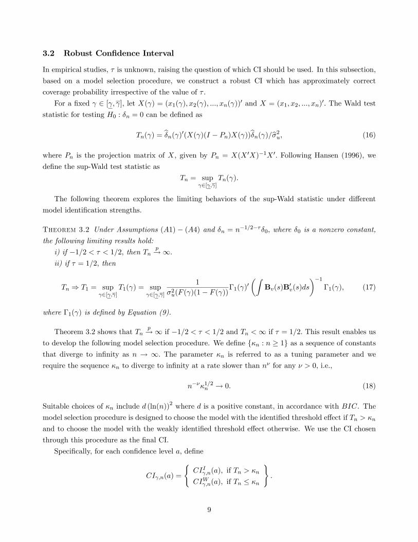
eyt = �0ext + �0next( ) + �0ezt + e�t = e�0 eA1t( ) + e�t; (21)

12

where e� = (�0; �0n; �0)0:Using Equation (21), for each ; we can de�ne

be�( ) = " nXt=2

eA1t( ) eA1t( )0#�1 " nXt=2

eA1t( )eyt# ; (22)

and the FGLS threshold estimator can be de�ned as

e n = arg min 2[ ; ]

(]SSRn( ));

where ]SSRn( ) is the sum of squared residuals given by

]SSRn( ) =nXt=2

�eyt( )� be�( )0 eA1t( )�2 : (23)

The following theorem establishes the limiting results of the FGLS estimator.

Theorem 4.2 Under Assumptions (A10); (A20); (A3) and (A4); the following results hold:

Case 1: if �1=2 < � < 1=2; then n1�2� je n � 0j = Op(1). Furthermore,n1�2�e�(e n � 0) = r� ) arg max

r2(�1;1)(�(r)� 1

2jrj);

where e� = �1 + �2� ��00 R Bv(s)B0v(s)ds�0� f0�2

; (24)

and �(r) is de�ned by Equation (7).

Case 2: if � = 1=2; then e n ) e ( 0; �0) and e ( 0; �0) is a random variable that maximizeseQ( ; 0; �0) whereeQ( ; 0; �0) = e�01( )

0@eG22( )� eG21( )eG23( )!0 eG11; eG13eG31; eG33

!�1 eG12( )eG32( )!1A�1 e�1( );

with

e�1( ) = e�( ) +0@eG22( )� eG21( )eG23( )

!0 eG11; eG13eG31; eG33!�1 eG12( )eG32( )

!1A �0;and e�( ) = e�2( )�

eG21( )eG23( )!0 eG11; eG13eG31; eG33

!�1 e�1( )e�3( )!; (25)

13

where the random matrix eG( ) =0B@ eG11( ); eG12( ); eG13( )eG21( ); eG22( ); eG23( )eG31( ); eG32( ); eG33( )

1CA and the random vector e�( ) =0B@ e�1( )e�2( )e�3( )

1CAare speci�ed in Lemma B.4 of the appendix.

Theorem 4.2 establishes the convergence results for the FGLS estimator e n: If �1=2 < � < 1=2, thethreshold value can be consistently estimated and its limiting distribution depends on the persistence

parameter �: Note that e� = �1 + �2��; implying that the FGLS estimator is more e¢ cient than thepro�led LS estimator when � 6= 0. The simulations in Section 5 demonstrate this result.

4.2 Generalized Sup-Wald Statistics

Testing for the existence of the threshold e¤ect in a cointegration regression is challenging since it is a

joint hypothesis problem (see Balke and Fomby, 1997). For example, when testing for the existence of

threshold e¤ects, the statistics based on error correction models (ECM) need to assume the model is

a cointegrating regression. Therefore, the rejection of the null hypothesis does not necessarily indicate

that there is a threshold e¤ect. It may mean that the regression is a spurious relationship. Thanks to

the robustness of the FGLS estimator, we can design a generalized sup-Wald test statistic based on this

estimator to test for the existence of threshold e¤ects, without any requirement on the stationarity of

the error term.

The null hypothesis is

H0 : �n = 0;

and the alternative is

H1 : �n 6= 0:

Under the null, after transformation, the model is

eyt = �0ext + �0ezt + e�t; (26)

while under the alternative, the transformed model is

eyt = �0ext + �0next( 0) + �0ezt + e�t= e�0 eA1t( 0) + e�t: (27)

Let fV1 = ( eX; eZ), then a generalized Wald statistic can be de�ned aseTn( ) = e�n( )0( eX( )(I � eP ( )) eX( ))e�n( )=e�2;

where eP ( ) is the projection matrix for eV1 and e�2 = ]SSRn( )=n:

14

The generalized sup-Wald statistic is de�ned as

eTn = sup 2[ ; ]

eTn( ):Theorem 4.3 Under Assumptions (A10); (A20); (A3), (A4) and H0 : �n = 0; the following limiting

result holds:

eTn ) eT = sup 2[ ; ]

eT ( )= sup

2[ ; ]

1

�2e�0( )

0@eG22( )� eG21( )eG23( )!0 eG11; eG13eG31; eG33

!�1 eG12( )eG32( )!1A�1 e�( );

where e�( ) is de�ned by Equation (25).Theorem 4.3 establishes the limiting distribution of the generalized sup-Wald test statistic, which is

nonstandard and we generate the critical values using a parametric bootstrap method. We �rst estimatebe�R using Equation (26) under the null. Then, we obtain the residual terms fbe�t(e n)gnt=2 using Equation(27) under the alternative. We draw a random variable e�bt from the sample fbe�t(e n)gnt=2 for all t = 2; :::; n;and generate a new sequence feybtgnt=1 by eybt = b�0Rext + b�0Rezt + e�bt : De�ne yb1 = y1 and ybt = eybt + b�ybt�1for all t = 2; :::; n: Let eT bn be the sup-Wald test calculated from the new data set fybt ; xt; zt; qtgnt=2.Under the null, the distribution of eT bn approximates the distribution of eTn: The bootstrap p-value isobtained by calculating the frequency of simulated eT bn that exceeds eTn when the number of simulationsis su¢ ciently large. Following Hansen (1996), one can show that the generated p-value converges to

the true size.

One can use the generalized sup-Wald statistic eTn to construct robust CIs for the threshold modelfollowing the procedures described in Section 3.2.

5 Simulations

This section demonstrates the �nite sample performance of the estimators and test statistics through

two simulation experiments.

Simulation 1: We examine the consistency of the pro�led LS estimator and the FGLS estimatorunder di¤erent model settings. We make comparisons between these two estimators to demonstrate

the advantage of the FGLS estimator when serial correlation and model endogeneity exist.

We consider the simple regression model

yt = �xt + �nxt(qt � 0) + �vt + ut;

where xt = xt�1 + vt and ut = �ut�1 + "t. The threshold variable qt is generated by an AR(1) process:

15

qt = 0:5qt�1 + et: The innovation processes vt; "t and et follow i.i.d. N(0; 1) and are independent of

each other. The true threshold value is set as 0 = 0 and the coe¢ cient � is set as 1: The parameter

� is set as 0 or 0:5, which controls the correlation between xt and ut: To check the impact of the serial

correlation of ut on the estimation, we set � as either 0; 1; 0:95 or �0:95. Moreover, we set the sizeof the threshold e¤ect as �n = 2n�1=2�� with � chosen as either 0 or 0:5, corresponding to the case

with identi�cation or the case with weak identi�cation. The number of replications is N = 1000: The

sample size n is set as 100; 200 or 400. We let the number of lags K = 5 in the FGLS estimator.8

Tables 1a and 1b report the mean square errors (MSE) of the pro�led LS and the FGLS estimators

for the threshold value and regression coe¢ cients, respectively.

Here insert Tables 1a and 1b

Speci�cally, Table 1a compares the performance of the pro�led LS and the FGLS estimators of the

threshold value under di¤erent model settings. Panel A displays the results when � = 0 (the case with

identi�cation). The pro�led LS estimator b is consistent when � < 1 (the error term ut is stationary)

no matter whether there exists regressor endogeneity or not, but it is inconsistent when � = 1 (the

error term ut is a unit root process). On the other hand, the FGLS estimator e is always consistent.Of particular interest is that the FGLS estimator performs better than the pro�led LS estimator when

serial correlation and regressor endogeneity exist, which is consistent with the theoretical result. Panel

B reports the results when � = 0:5 (the case with weak identi�cation). Both pro�led LS and FGLS

estimators are inconsistent since their MSE do not converge to zero as the sample size increases to

in�nity. However, the FGLS estimators still have smaller MSE than the pro�led LS estimators in

most cases. Similar conclusions can be drawn from Table 1b, which reports the MSE of the regression

coe¢ cient estimators.

Simulation 2: In this experiment, we examine the performance of the sup-Wald test statistics andthe model selection procedure. The data generating process is the same as in Simulation 1, but we

consider an additional case with �n = 0 to evaluate the size performance of the test statistics.

Table 2a reports the size performance of the sup-Wald statistic Tn and the generalized sup-Wald

statistic eTn; which are based on the pro�led LS estimator and the FGLS estimator, respectively. Com-paring Panel A with Panel B, one can see that eTn has better size performance than Tn when serialcorrelation or regressor endogeneity exists. In an unreported result with the sample size n = 1000, the

rejection rate of eTn is close to the size, but not for Tn: Thus, we suggest that the generalized sup-Waldstatistic eTn should be used in practice.

Here insert Table 2a

Tables 2b through 2d report the power performance for Tn and eTn with di¤erent sample sizes. Inall three tables, Panel A shows the results for the case with identi�cation and Panel B shows the case

with weak identi�cation.8Other values for K; such as 10 and 15, are also applied with little change in the results.

16

Here insert Tables 2b, 2c and 2d

When the threshold e¤ect is identi�ed, both Tn and eTn seem to be consistent since their power

converges to one as the sample size increases. In particular, eTn performs better than Tn when thereexists serial correlation, model endogeneity or both; the advantage of the generalized sup-Wald statistic

is con�rmed.

However, when the threshold e¤ect is only weakly identi�ed, both statistics seem to have low power

even when the sample size is 400, which is consistent with the theoretical results. In practice, one may

use the model selection procedure described in Section 3.2 to detect the case with weak identi�cation.

We choose (ln(n))2 as the tuning parameter �n and judge that the model is weakly identi�ed if Tn oreTn is smaller than �n. From the columns corresponding to (ln(n))2 in Tables 2b-2d, one can �nd that

the model selection procedure based on eTn works very well in all cases.6 Conclusion

In the literature, statistical theory for threshold models with stationary explanatory variables has been

well developed by Hansen (1996, 2000). However, in empirical macroeconomics and �nance, many

explanatory variables are nonstationary. This paper establishes statistical theory for threshold models

with nonstationary regressors under the diminishing threshold e¤ect assumption. Our work can also

be related to the literature of nonlinear cointegration. The proposed approach o¤ers some �exibility of

the cointegrating structure such that it can capture threshold e¤ects in the long-run relationship. The

merits of the method have been successfully demonstrated through Monte Carlo simulations.

There are several directions open for further work. First, it may be interesting to develop a more

general model with multiple threshold e¤ects, each with a di¤erent identi�cation strength. A sequential

procedure can be applied to determine the number of regimes and their identi�cation strengths. Second,

the model can be extended to allow for stationary regressors. Moreover, there are many interesting

applications. For example, one can use the model to study the regime-sensitive Taylor rule (Taylor,

1993), where the dependent variable yt could be the short-term interest rate, the explanatory variables

xt could be macroeconomic variables such as the in�ation rate and the unemployment rate, and the

threshold variable qt could be the GDP growth rate. Another application is to model the regime-

dependent predictability of the fundamental ratios, such as the dividend-price ratio and the earning-

price ratio, to equity returns. The threshold variable could be a variable indicating the status of the

economy. All these are left for future studies.

References

Andrews, D.W.K. (1993). Tests for parameter instability and structural change with unknown change

point. Econometrica, 61, 821-856.

17

Andrews, D.W.K. and C. J. McDermott (1995). Nonlinear econometric models with deterministically

trending variables. Review of Economic Studies, 62(3), 343-60.

Balke, N. and T. Fomby (1997). Threshold cointegration. International Economics Review, 8, 627-645.

Bierens H. and L. Martins (2010). Time-varying cointegration. Econometric Theory, 26, 1453-1490.

Billingsley, P. (1999). Convergence of probability Measures, 2nd ed, Wiley, New York.

Cai, Z., Q. Li and J.Y. Park (2009). Functional-coe¢ cient models for nonstationary time series data.

Journal of Econometrics, 148, 101-113.

Campbell, J.Y. and M. Yogo (2006). E¢ cient tests of stock return predictability. Journal of Financial

Economics, 81, 27-60.

Caner, M. and B.E. Hansen (2001). Threshold autoregression with a unit root. Econometrica, 69,

1555-1596.

Caner, M. (2007). Boundedly pivotal structural change tests in continuous updating GMM with

strong, weak identi�cation and completely unidenti�ed cases. Journal of Econometrics, 137,

28-67.

Chen, H. (2013). Robust Estimation and Inference for Threshold Models with Integrated Regressors.

Working Papers, Xiamen University. Available at SSRN: http://ssrn.com/abstract=2287442.

Cheng, X. (2008). Robust con�dence intervals in nonlinear regression under weak identi�cation.

Manuscript, Department of Economics, Yale University.

Chan, K.S. (1993). Consistency and limiting distribution of the least squares estimator of a threshold

autoregressive Model. Annals of Statistics, 21, 520-533.

Choi, C.Y., L. Hu and M. Ogaki (2008). Robust estimation for structural spurious regressions and a

Hausman-type cointegration test. Journal of Econometrics, 142, 327-351.

Choi, In and P. Saikkonen (2010). Test of nonlinear cointegration. Econometric Theory, 26, 682-709.

Durlauf, S.N. and P.A. Johnson (1995). Multiple regimes and cross-country growth behaviour. Journal

of Applied Econometrics, 10, 365�84.

Elliott, G. and U.K. Müller (2007). Con�dence sets for the date of a single break in linear time series

regressions. Journal of Econometrics, 141(2), 1196-1218.

Gao, J., M. L. King, Z. Lu and D. Tjøstheim (2009a). Speci�cation testing in nonstationary time

series autoregression. Annals of Statistics, 37, 3893-3928.

Gao, J., M. L. King, Z. Lu and D. Tjøstheim (2009b). Nonparametric speci�cation testing for nonlinear

time series with nonstationarity. Econometric Theory, 25, 1869-1892.

18

Gonzalo, J. and J. Pitarakis (2002). Estimation and model selection based inference in single and

multiple threshold models. Journal of Econometrics, 110, 319-352.

Gonzalo, J. and J.Y. Pitarakis (2006). Threshold e¤ects in cointegrating regressions. Oxford Bulletin

of Economics and Statistics, 813-833.

Gonzalo, J. and J.Y. Pitarakis (2012). Regime speci�c predictability in predictive regressions. Journal

of Business and Economic Statistics, 30(2), 229-241.

Hansen, B.E. (1996). Inference when a nuisance parameter is not identi�ed under the null hypothesis.

Econometrica, 64, 413-430.

Hansen, B.E. (1997). Inference in TAR models. Studies in Nonlinear Dynamics and Econometrics, 2,

1-14.

Hansen, B.E. (2000). Sample splitting and threshold estimation. Econometrica, 68, 575-603.

Karlsen H.A., T. Myklebust and D. Tjøstheim (2007). Nonparametric estimation in a nonlinear

cointegration type model. Annals of Statistics 35 (1), 252-299.

Kasparis, I. (2008). Detection of functional form misspeci�cation in cointegrating relations. Econo-

metric Theory, 24, 1373-1404.

Li D. and S. Q. Ling (2012). On the least squares estimation of multiple-regime threshold autoregres-

sive models. Journal of Econometrics, 167, 240�253.

Marmer, V. (2008). Nonlinearity, nonstationarity, and spurious forecasts, Journal of Econometrics,

142(1), 1-27.

Park, J.Y. (1992). Canonical cointegrating regressions. Econometrica, 60, 119-143.

Park, J.Y. and S. Hahn (1999). Cointegration regression with time varying coe¢ cients. Econometric

Theory, 15, 664-703.

Park, J.Y. and P.C.B. Phillips (2001). Nonlinear regressions with integrated time series. Econometrica,

69(1), 117-161.

Perron, P. and T. Yabu (2009). Testing for shifts in trend with an integrated or stationary noise

component. Journal of Business and Economics Statistics, 27(3), 369-396.

Phillips, P.C.B. and S.N. Durlauf (1986). Multiple time series regression with integrated processes.

Review of Economic Studies, 53, 474-95.

Phillips, P.C.B. and J.Y. Park (1988). Asymptotic equivalence of ordinary least squares and general-

ized Least squares in regressions with integrated regressors. Journal of the American Statistical

Association, 83, 111-115.

19

Phillips, P.C.B. and B.E. Hansen (1990). Statistical inference in instrumental variables regression

with I(1) processes. Review of Economic Studies, 57, 99-125.

Phillips, P.C.B. and D.J. Hodgson (1994). Spurious regression and generalized least squares. Econo-

metric Theory, 10, 957�958.

Potter, S.M. (1995). A nonlinear approach to US GNP. Journal of Applied Econometrics, 2, 109�25.

Saikkonen, P. (1991). Asymptotically e¢ cient estimation of cointegration regressions. Econometric

Theory, 7, 1-20.

Seo, M. and O. Linton (2007). A smoothed least squares estimator for threshold regression models.

Journal of Econometrics, 141, 704�735.

Shao, Q. and C. Lu (1987). Strong approximation for partial sums of weakly dependent random

variables. Scientia Sinica, 15, 576-587.

Shi, X. and P.C.B. Phillips (2012). Nonlinear cointegration regression under weak identi�cation.

Econometric Theory, 28(1), 1-39.

Stock, J.H. and M.W. Watson (1993). A simple estimator of cointegrating vectors in higher order

integrated systems. Econometrica, 61, 783-820.

Taylor, J. B (1993). Discretion versus policy rules in practice. Carnegie-Rochester Conference Series

on Public Policy, 39, 195-214.

Tsay, R. S. (1998). Testing and modeling multivariate threshold models. Journal of the American

Statistical Association, 93, 1188-1202.

Wang, Q. and P.C.B. Phillips (2009a). Structural nonparametric cointegrating regression. Economet-

rica, 77(6), 1901-1948.

Wang Q. and P.C.B. Phillips (2009b). Asymptotic theory for local time density estimation and

nonparametric cointegrating regression. Econometric Theory, 25, 710-738.

Xiao, Z. (2009). Functional-coe¢ cient cointegration models. Journal of Econometrics, 152(2), 81-92.

Yu, P. (2012). Likelihood estimation and inference in threshold regression. Journal of Econometrics,

167, 274�294.

20

AppendixIn this appendix, Part A provides the proofs related to the basic model while Part B is for the generalized model.

To save space, we skip the details for some intermediary results and a more detailed presentation can be found in

Chen (2013).

Part ALemma A.1: Under Assumptions (A1)�(A3), for any 2 [ ; ]; we have 1p

n

P[ns]t=1 It(qt � )ut ) �uW (s; F ( )):

Lemma A.2: Under Assumptions (A1)� (A4), for any 2 [ ; ]; we have

1

n

nXt=1

xtIt( )ut ) �u

ZBv(s)dW (s; F ( )):

Lemma A.3: Under Assumptions (A1)� (A4), for any 2 [ ; ]; as n!1; we havea) n�2

Pnt=1At( )A

0t( ) =M( ) + oa:s(1);

b) n�1Pn

t=1At( )ut ) �u

RBv(s)dW (s)R

Bv(s)dW (s; F ( ))

!;

where At( ) is de�ned in Equation (5) and M( ) =

RBv(s)B

0v(s)ds F ( )

RBv(s)B

0v(s)ds

F ( )RBv(s)B

0v(s)ds F ( )

RBv(s)B

0v(s)ds

!:

Lemma A.4: Under Assumptions (A1)� (A4); we have

n(b�( 0)� �)) �uM( 0)�1

RBv(s)dW (s)R

Bv(s)dW (s; F ( 0))

!:

For any 6= 0; if �1=2 < � < 1=2; we have

n�+1=2(b�( )� �))M( )�1�( ; 0; �0);

if � = 1=2;

n(b�( )� �)) �uM( )�1

RBv(s)dW (s)R

Bv(s)dW (s; F ( ))

!+M( )�1�( ; 0; �0);

where

�( ; 0; �0) = �

(F ( )� F ( 0))RBv(s)B

0v(s)ds

(F ( )� F ( 0 ^ ))RBv(s)B

0v(s)ds

!�0:

Proof of Lemma A.1-A.4: The proofs are standard and are skipped here.

Lemma A.5: If �1=2 < � < 1=2; we have b n p! 0:

Proof: To establish the consistency of b n, we need to prove Pr(jb n � 0j > ") ! 0 for any " > 0: Denote

B(�) = f : j � 0j > "g and B(�) = [ ; ]nB(�): By the de�nition of b n; we havePr(jb n � 0j > ") = Pr

inf

2B(�)SSRn( ) < inf

2B(�)SSRn( )

!� Pr

�inf

2B(�)SSRn( ) < SSRn( 0)

�= Pr( inf

2B(�)n2��1(SSRn( )� SSRn( 0)) < 0):

Thus, to prove Pr(je n � 0j > ") ! 0; it su¢ ces to show that inf 2B(�) n2��1(SSRn( ) � SSRn( 0)) > 0 with

probability 1.

21

Rewrite Equation (2) as a matrix compacted form: Y = X 0� + X( 0)0�n + u; where Y;X;X( 0) and u stack

yt; xt; xtI(qt � 0) and ut; respectively. Denote X�( ) = (X( ); X �X( )) and de�ne its projection matrix P � =X�( )(X�( )0X�( ))�1X�( )0: By some simple algebra, we have

SSRn( ) = Y0(I � P � )Y = �0nX( 0)0(I � P � )X( 0)�n + 2�0nX( 0)0(I � P � )u+ u0(I � P � )u;

where the second equation uses the fact that X 0(I � P � ) = 0; since X is a linear combination of (X( ); X �X( )):When = 0; we have SSRn( 0) = u

0(I � P � 0)u; and it follows that

n2��1(SSRn( )� SSRn( 0)) = n�1+2��0nX( 0)0(I � P � )X( 0)�n + n�1+2�2�0nX( 0)0(I � P � )u

+n�1+2� (u0(I � P � )u� u0(I � P � 0)u) � S1 + S2 + S3; say. (A.1)

Next, we will show that S1 + S2 + S3 uniformly converges to a function b( ) which is positive for any 2 B(�):Given �1=2 < � < 1=2, by Lemma A.3, it can be shown that

S2 = n�1=2+�2

�n1=2+��n

�0 1nX( 0)

0(I � P � )u = n�1=2+�2�001

nX( 0)

0(I � P � )u = Op(n�1=2+� )p! 0;

S3 = n�1+2� (u0(I � P � )u� u0(I � P � 0)u) = n

�1+2� (u0P � 0u� u0P � u) = Op(n

�1+2� )p! 0:

Using a similar argument of Lemma A.5 in Hansen(2000), we can show, for any � 0;

S1 = n�1+2��0nX

0( 0)(I � P � )X( 0)�np! (F ( 0)� F ( 0)F ( )�1F ( 0))�00

�ZBv(s)B

0v(s)ds

��0 � b1( )

uniformly: Since (F ( 0)�F ( 0)F ( )�1F ( 0)) � 0 andRBv(s)B

0v(s)ds is positive de�nite random matrix, b1( ) � 0

and the equality holds if and only if = 0:

For � 0; we can show

S1p! (F ( 0)� F ( ))�00

�ZBv(s)B

0v(s)ds

��0 � b2( )

uniformly, where b2( ) � 0 and the equality holds if and only if = 0: De�ne b( ) = b1( )I( � 0)+b2( )I( � 0),and we have shown that

n�1+2� (SSRn( )� SSRn( 0))p! b( )

uniformly for any 2 [ ; ] and b( ) is strictly positive when 2 B(�): Thus, Pr(inf 2B(�) n2��1(SSRn( ) �SSRn( 0)) > 0)! 1:

Proof of Theorem 3.1: We �rst prove the limiting results for the case with �1=2 < � < 1=2: Let an = n1�2� :To prove b n converge to 0 with rate an; we need to prove that anjb n� 0j = Op(1), or there exists a constant v > 0;limn!1 Pr(jb n � 0j � v=an) = 1: For any B > 0; de�ne VB = f : j � 0j < Bg: When n is large enough, we havev=an < B: Since b n p! 0 according to Lemma A.5, Pr(fb n 2 VBg) p! 1: Therefore, we only need to examine the

limiting behavior of in VB :

De�ne a subset VB(v) = f : v=an < j � 0j < Bg: Thus, VB(v) � VB : To prove Pr(jb n � 0j � v=an) = 1; wejust need to prove Pr(b n 2 VB(v)) = 0: Let b� and b� be the estimation of b�(b n) and b�(b n): Also, we denote SSR�n( ) =Pn

t=1(yt�b�0At( ))2 and SSR�n( 0) =Pnt=1(yt�b�0At( 0))2: By the de�nition of b n; we have SSR�n(b n) � SSR�n( 0):

Hence, it su¢ ces to prove that for any 2 VB(v); SSR�n( ) > SSR�n( 0) with probability 1.

22

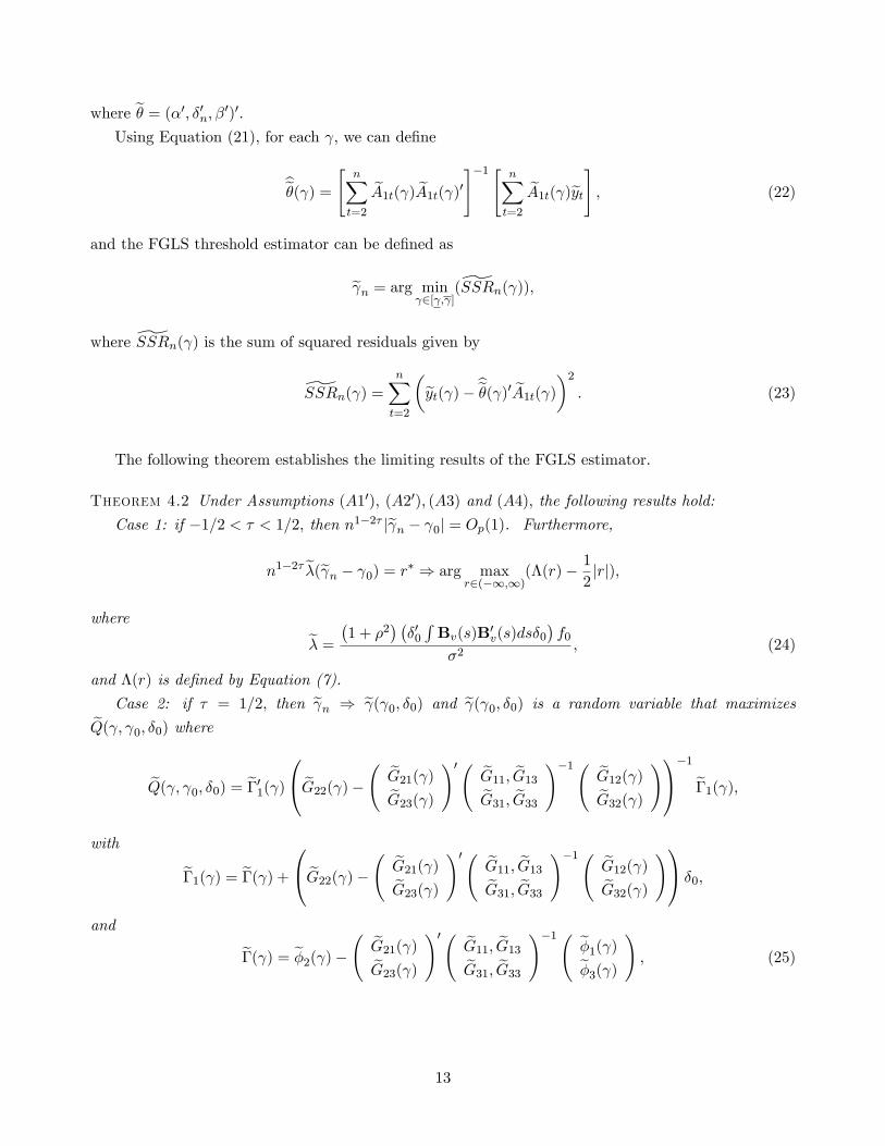
We consider the case of > 0 �rst. Using an argument of symmetry, we can, without loss of generality, prove

the result for the case of < 0: Note that

SSR�n( )� SSR�n( 0) =nXt=1

(yt � b�0At( ))2 � nXt=1

(yt � b�0At( 0))2=

nXt=1

�0n(xt( )� xt( 0))(xt( )� xt( 0))0�n � 2�0nnXt=1

(xt( )� xt( 0))u+ 2b�0 nXt=1

(xt( )� xt( 0))(xt( )� xt( 0))0(b� � �)+2

nXt=1

(b� + �n)0(xt( )� xt( 0))(xt( )� xt( 0))0(b� � �n) + 2(�0n � b�0) nXt=1

(xt( )� xt( 0))u

� R1 �R2 +R3 +R4 +R5; say. (A.2)

Next, we show that R1+R2+R3+R4+R5

an( � 0)converges to a positive random variable almost surely by studying the

limiting behavior for each term speci�cally. First, note that

R1an

=1

an

nXt=1

�0n(xt( )� xt( 0))(xt( )� xt( 0))0�n = (F ( )� F ( 0))�00ZBv(s)B

0v(s)ds�0 + op(1)

= f( 0)( � 0)�00�Z

Bv(s)B0v(s)ds

��0 + op(1):

The last equation uses the �rst-order Taylor approximation of F ( ) around 0:

Noting that v=an < j � 0j < B and an = n1�2� with � < 1=2; We havepv <

panp(j � 0j): Thus, there

exists k > 0; such that

R2an( � 0)

=2�00

1n

Pnt=1(xt( )� xt( 0))upan( � 0)

= Op(1

panp(j � 0j)

) � k=pv:

For any B ! 0+, there exists v > 0 and N; such that k=pv < f( 0)�

00

RBv(s)B

0v(s)ds�0 with probability 1 and

v=an < B when n > N: Therefore, for any 2 VB(v), we have

R1an( � 0)

� R2an( � 0)

> 0; (A.3)

Furthermore, from Lemma A.4, we have n�+1=2((b�� ) = Op(b n � 0) and n�+1=2(b�n � �n) = Op(b n � 0), thusR3

an( � 0)=2n�+1=2b�0nn�2Pn

t=1(xt( )� xt( 0))(xt( )� xt( 0))0n�+1=2(b� � �)( � 0)

= Op(b n � 0) = op(1); (A.4)

R4an( � 0)

=2n�+1=2(b� + �n)0n�2Pn

t=1(xt( )� xt( 0))(xt( )� xt( 0))0n�+1=2(b� � �n)( � 0)

= Op(n�+1=2(b� � �n) = Op(b n � 0) = op(1); (A.5)

R5an( � 0)

=2n2� (�0n � b�0)n�1Pn

t=1(xt( )� xt( 0))u( � 0)

= Op(n�+1=2(b� � �n)n��1=2) = op(1): (A.6)

Combining the results of Equations (A.3) through (A.6), we have SSR�n( )�SSR

�n( 0)

an( � 0)> 0 with probability 1 for any

2 VB(v) and > 0: Similarly, we can prove SSR�n( ) > SSR�n( 0) when < 0 and 2 VB(v) with probability1.

23

Next, we study the limiting distribution for the estimator b : Given �1=2 < � < 1=2; b is a consistent estimatorwith convergence rate an, thus, we could focus on its asymptotic behavior in the neighborhood of the true thresholds.

Let = 0 +!

an. By the de�nition of b n; we have

an(b n � 0) = !� = arg min!2(�1;1)

�SSR�n( 0 +

!

an)� SSR�n( 0)

�:

By Equation (A.2), we know SSR�n( 0+!

an)�SSR�n( 0) = R1�R2+R3+R4+R5; with replaced by 0+

!

an:

Next, we turn to study the limiting behavior for each term. We only provide the proof for the case where ! > 0, as

the proof for the case with ! � 0 is analogous. Given ! > 0; we have

R1 = �0n

nXt=1

�xt( 0 +

!

an)� xt( 0)

��xt( 0 +

!

an)� xt( 0)

�0�n

= n1�2��00n�2

nXt=1

�xt( 0 +

!

an)� xt( 0)

��xt( 0 +

!

an)� xt( 0)

�0�0

= n1�2��00(F ( 0 +!

an)� F ( 0))

�ZBv(s)B

0v(s)ds

��0 + op(1)

p! f( 0)!�00

�ZBv(s)B

0v(s)ds

��0: (A.7)

Note that the last equation uses the �rst-order Taylor expansion of F ( 0 +!

an) around 0: For R2; we have

R2 = �2nXt=1

�0n

�xt( 0 +

!

an)� xt( 0)

�ut = �2n1=2��00

1

n

nXt=1

�xt( 0 +

!

an)� xt( 0)

�ut

) �2pan�00�uZBv(s)d

�W (s; F ( 0 +

!

an))�W (s; F ( 0))

�= �2pan�00�u

�J1(F ( 0 +

!

an))� J1(F ( 0))

�: (A.8)

Note that J1(�) =RBv(s)dW (s; �) is a mean-zero Gaussian process with an almost surely continuous sample

path and with the covariance kernel

E(J1(�1)J1(�2)) = (�1 ^ �2)ZBv(s)B

0v(s)ds:

Thus, D(!) =pan�

00�u

�J1(F ( 0 +

!

an))� J1(F ( 0))

�is also a Brownian motion with

V ar(D(!)) = �2uan(F ( 0 +!

an)� F ( 0))�00

ZBv(s)B

0v(s)ds�0

= �2uf0!

ZBv(s)B

0v(s)ds+ op(1):

By Equations (A.4) to (A.6); we have R3 + R4 + R5 = !op(1) = op(1): Combining the convergence results of

24

Equations (A.7) and (A.8), we have

SSR�n ( )� SSR�n ( 0) ) f0!�00

ZBv(s)B

0v(s)ds�0 � 2D(!)

= f0!�00

ZBv(s)B

0v(s)ds�0 � 2�u

sf0!�

00

ZBv(s)B0v(s)ds�0�1(!);

where �1(!) is a standard Brownian motion on [0;1): Making the change of variables as follows

! =�2u

�00�RBv(s)B0v(s)ds

��0f0

r;

we have

SSR�n ( )� SSR�n ( 0)) 2�2u(r

2� �1(r)): (A.9)

Using continuous mapping theorem, the asymptotic distribution of b can be expressed asn1�2��(b � 0) = r� ) arg max

r2(0;1)(�1(r)�

1

2jrj):

Lastly, we establish the limiting results for b n when � = 1=2; i.e., the threshold is only weakly identi�ed: By thede�nition of b n, we have b n = argmin 2[ ; ] SSRn( ) = argmax 2[ ; ](SSRn � SSRn( )); where SSRn is de�nedas the sum of squared residuals by regressing yt to xt: By some standard algebra, we have

SSRn � SSRn( ) = Y 0(I � Pn)X( )(X 0( )(I � Pn)X( ))�1X 0( )(I � Pn)Y;

where X( ) = (x1( ); x2( ); :::; xn( ))0 and X = (x1; x2; :::; xn)0: Pn = X(X

0X)�1X 0 is the projection matrix of X.

De�ne �n( ) = n�1X 0( )(I � Pn)Y: By substituting the true model Y = X�+X( 0)�n + u; it can be shown that

�n( ) = n�1X 0( )X( 0)�n � n�1X 0( )X(X 0X)�1X 0X( 0)�n + n

�1X 0( )(I � Pn)u:

Given � = 1=2; we have n�n = �0. By Lemma A.3, it can be shown that

�n( )) �u

ZBv(s)d (W (s; F ( ))� F ( )W (s)) + (F ( ^ 0)� F ( )F ( 0))

�ZBv(s)B

0v(s)ds

��0 � �1( ):

Since

n�2X 0( )(I � Pn)X( ) = n�2X 0( )X( )� n�2X 0( )X(X 0X)�1X 0X( )) F ( )(1� F ( ))ZBv(s)B

0v(s)ds;

by continuous mapping theorem, we can show that

(SSRn � SSRn( )) = �0n( )(X0( )(I � Pn)X( )=n2)�1�n( )

) 1

F ( )(1� F ( ))�01( )

�ZBv(s)B

0v(s)ds

��1�1( ) = Q( ; 0; �0):

25

Proof of Theorem 3.2: Note that

Tn( ) = b�n( )0(X( )(I � P ( ))X( ))b�n( )=b�2u= (I � Pn)Y 0X( )(X 0( )(I � Pn)X( ))�1X 0( )(I � Pn)Y=b�2u= �n( )

0 �n�2X( )0X( )� n�2X( )0X(X 0X)�1XX( )��1

�n( )=b�2u: (A.10)

By Lemma A.3, we have

n�2X( )0X( )� n�2X( )0X(X 0X)�1XX( )a:s:!�F ( )� F ( )2

� ZBv(s)B

0v(s)ds:

Next, we consider the limiting result for �n( ) for di¤erent � : When �1=2 < � < 1=2; we have

�n( ) =1

nX 0( )(I � Pn)Y =

1

nX 0( )u� 1

nX 0( )X(X 0X)�1X 0u+

1

nX 0( )X( 0)�n �

1

nX 0( )X(X 0X)�1X 0X( 0)�n

) �u

Z 1

0

Bv(s)d (W (s; F ( ))� F ( )W (s)) + n1=2�� (F ( ^ 0)� F ( )F ( 0))�Z

Bv(s)B0v(s)ds

��0

= Op(n1=2�� )

p!1:

It follows that Tn( ) = Op(n1�2� )p!1: When � = 1=2; we have

�n( ) =1

nX 0( )u� 1

nX 0( )X(X 0X)�1X 0u+

1

nX 0( )X( 0)�n �

1

nX 0( )X(X 0X)�1X 0X( 0)�n

) �( ) + (F ( ^ 0)� F ( )F ( 0))�Z

Bv(s)B0v(s)ds

��0 = �1( ):

It follows that

Tn( ))1

�2uF ( )(1� F ( ))�01( )

�ZBv(s)B

0v(s)ds

��1�1( ):

Proof of Theorem 3.3: We prove the equality by showing the following two inequalities: AsySZ (a) � 1� aand AsySZ (a) � 1� a hold simultaneously. We �rst consider the proof of AsySZ (a) � 1� a:By the de�nition ofAsySZ (a) as Equation (20), we can �nd a parameter sequence (�n; n) such thatAsySZ (a) =

lim infn!1 Pr(�n; n)( n 2 CI ;n(a)): Let fbng be a subsequence of fng such thatAsySZ (a) = limn!1 Pr(�bn ; bn )( bn 2CI ;bn(a)): Denote �

�0 = n�n where �

�0 2 R[f�1;1g: Because the Euclidean space is complete, we can always �nd

a subsequence fcng of fbng such that�cn�cn ; cn

�! (��0; 0):

If � = 1=2; we have ��0 = nn�1=2��0 = �0 2 R: By Theorem 3.2, we have Tn = Op(n1�2� ) = Op(1) < �n with

probability one. Thus, CI ;n(a) = CIW ;n(a); and

AsySZ (a) = limn!1

Pr(�cn ; cn )( cn 2 CI ;cn(a)) = limn!1

Pr(�cn ; cn )(jb cn � cn j � bqW ;1�a)� lim

n!1Pr(�cn ; cn )(jb cn � cn j � bqW ;1�a( 0; �0)) = 1� a:

The inequality uses the fact that bqW ;1�a = sup 2[ ; ] sup�2R qW ;1�a( ; �): The last equation uses the fact that jb cn� cn jconverges to jb ( 0; �0) � 0j and bqW ;1�a( 0; �0) is de�ned as the (1 � a) quantile of the limiting distribution ofjb ( 0; �0)� 0j:If �1=2 < � < 1=2; ��0 = nn�1=2��0 = n1=2��0 = �1: Note that n��1=2n ! 0 for any � > 0; we have

26

Tn = Op(n1�2� ) > �n with probability approaching one. Thus, CI ;cn(a) = CI

I ;cn(a) and

AsySZ (a) = limn!1

Pr(�cn ; cn )( cn 2 CI ;cn(a)) = limn!1

Pr( cn 2 CII ;cn(a)) = lim

n!1Pr(LR( cn) � q

I1��):

As LRn( n)) supr2(�1;1)(2�(r)�jrj); LRcn( cn) converges to supr2(�1;1)(2�(r)�jrj) and qI1�� is the 1�aquantile of supr2(�1;1)(2�(r)� jrj): Thus,

AsySZ (a) = limn!1

Pr(LR( cn) � qI1��) � 1� a:

Next, we consider the other side AsySZ (a) � 1 � a: Let �n = n�1=2�0 and n = 0 with �0 2 R=f0g: Byde�nition, we have

AsySZ (a) � lim infn!1

Pr(�0; 0)( 0 2 CI ;n(a)):

When �n = n�1=2�0, we have Tn = Op(n1�2� ) = Op(n) > �n with probability approaching one. Thus, CI ;n(a) =

CII ;n(a); and

lim infn!1

Pr(�n; 0)( 0 2 CI ;n(a)) = lim infn!1

Pr( 0 2 CII ;n(a)) = lim infn!1

Pr(LRn( 0) � qI1��) = 1� a:

where the last equality holds because LRn( 0)) supr2(�1;1)(2�(r)� jrj).

Part B

De�ne the moment functionals for the stationary regressors zt

h( ) = E(ztI(qt � )); h1( ) = E(ztI(qt�1 � )); h2( ) = E(zt�1I(qt � ));

H = E(ztz0t); H1 = E(ztz

0t�1):

Lemma B.1; Under Assumptions A10; A20; A3 and A4; for any 2 [ ; ]; as n!1;a) n�3=2

Pnt=1 ztx

0t( ) = h( )

RB0v(s)ds+ op(1);

b) n�3=2Pn

t=1 ztx0t�1( ) = h1( )

RB0v(s)ds+ op(1);

c) n�3=2Pn

t=1 zt�1x0t( ) = h2( )

RB0v(s)ds+ op(1);

d) n�1Pn

t=1 ztz0t = H + op(1);

e) n�1Pn

t=1 ztz0t�1 = H1 + op(1):

Lemma B.2: Under Assumptions A10; A20; A3 and A4, for any 2 [ ; ] and � = F ( ) as n!1;a) : n�1=2

Pnt=1 I(qt � )"t ) �W (s; �);

b) : n�1=2Pn

t=1 I(qt�1 � )"t ) �W1(s; �);

c) : n�1Pn

t=1 xt( )0"t ) �

RB0v(s)dW (s; �);

d) : n�1Pn

t=1 xt�1( )0"t ) �

RB0v(s)dW1(s; �);

e) : n�1=2Pn

t=1 zt"t ) �J2;

f) : n�1=2Pn

t=1 zt�1"t ) �J3;

where J2 and J3 are Gaussian random variable with mean zero and variance H: W (s; �) and W1(s; �) are two

two-parameter Brownian motions.

Proof of Lemma B.1-B.2: The proofs are standard and are skipped for space considerations.

27

Lemma B.3: If �1=2 < � < 1=2; under Assumptions A10; A20; A3 and A4, we have b n p! 0 for any � 2 (�1;1]:

Proof: We conduct the proof by considering two cases according to the value of �: When � < 1; ut = �0zt + �tis stationary process. The proof is similar to Lemma A.5 and is skipped for brevity. When � = 1; ut = �0zt + �t

is nonstationary since �t is a unit root process. Using a similar argument of Lemma A.5, we only need to show

that n�1+2� (SSRn( )� SSRn( 0)) uniformly converges to a function b( ) which is positive when 2 B(�); whereB(�) = f : j � 0j > "g for any " > 0: Note that Equation (A.1) still holds, i.e., n�1+2� (SSRn( )� SSRn( 0)) =S1 + S2 + S3. Next, we will show that both S2 and S3 converge to zero but S1 uniformly converges a function b( )

which is positive when 2 B(�):First, note that the stationary component �0zt of ut is asymptotically negligible, implying that

S3 = n�1+2� (u0(I � P � )u� u0(I � P � 0)u) = n

�1+2� (�0P � � � �0P � 0�) + op(1):

Denote B�(s) as a Brownian motion such that 1pn�[ns] ) B�(s): By Lemma B.1, we have

n�2�0X�( )(X�( )0X�( ))�1X�( )0� = n�2�0X�( )(n�2X�( )0X�( ))�1n�2X�1 ( )

0�

=

F ( )

R 10Bv(s)B�(s)ds

(1� F ( ))R 10Bv(s)B�(s)ds

!0 F ( )

RBv(s)B

0v(s)ds; 0

0; (1� F ( ))RBv(s)B

0v(s)ds

!�1 F ( )

R 10Bv(s)B�(s)ds

(1� F ( ))R 10Bv(s)B�(s)ds

!+ op(1)

=

F ( )

R 10Bv(s)B�(s)ds

(1� F ( ))R 10Bv(s)B�(s)ds

!0 (RBv(s)B

0v(s)ds)

�1 R 10Bv(s)B�(s)ds

(RBv(s)B

0v(s)ds)

�1 R 10Bv(s)B�(s)ds

!+ op(1)

=

�Z 1

0

Bv(s)B�(s)ds

�0�ZBv(s)B

0v(s)ds

��1�Z 1

0

Bv(s)B�(s)ds

�+ op(1);

which is unrelated to : Thus, �0P � ��0P � 0� = op(1) and it follows that S3 = n�1+2� (�0P � ��0P � 0�)+op(1) = op(1):

To prove S2 converge to zero almost surely, we �rst consider the case where > 0: For the case where � 0;theproof is similar and not repeated here. Given > 0; We have

n�2X 0( )X( 0) = n�2X 0( 0)X( 0) = F ( 0)

ZBv(s)B

0v(s)ds+ op(1);

n�2X( 0)0(X �X( )) = 0;

n�2(X �X( 0))0X( ) = (F ( )� F ( 0))ZBv(s)B

0v(s)ds+ op(1):

It follows that

n�2X�( 0)0X�( ) =

F ( 0)

RBv(s)B

0v(s)ds; 0

(F ( )� F ( 0))RBv(s)B

0v(s)ds; (1� F ( ))

RBv(s)B

0v(s)ds

!+ op(1):

Furthermore, it can be shown that

n�1+2�2�0nX( 0)0� = 2n1=2+��00n

�2nXt=1

xt( 0)� = 2n1=2+��00

F ( 0)

RBv(s)B�(s)ds

(1� F ( 0))RBv(s)B�(s)ds

!+ op(1);

28

and

2n�1+2��0nX( 0)0P � � = 2n

1=2+��0

F ( 0)

RBv(s)B

0v(s)ds; 0

(F ( )� F ( 0))RBv(s)B

0v(s)ds; (1� F ( ))

RBv(s)B

0v(s)ds

!

F ( )RBv(s)B

0v(s)ds; 0

0; (1� F ( ))RBv(s)B

0v(s)ds

!�1 F ( )

RBv(s)B�(s)ds

(1� F ( ))RBv(s)B�(s)ds

!

= 2n1=2+��00

F ( 0)

RBv(s)B

0v(s)ds

(1� F ( 0))RBv(s)B

0v(s)ds

!+ op(1):

Thus,

S2 = n�1+2�2�0nX( 0)

0(I � P � )� = n�1+2�2�0nX( 0)0� � 2n�1+2��0nX( 0)0P � � + op(1) = op(1):

Using a similar argument in Lemma A.5, we can show S1p! b( ) uniformly and b( ) is strictly positive when

2 B(�): Combining the convergence results for S1; S2 and S3, we complete the proof.

Proof of Theorem 4.1: Under Assumption A10, the model can be rewritten as

yt = �0xt + �

0nxt( 0) + ut = �

01x�t (b ) + ��t ;

where x�t (b ) = (xt(b )0; x0t � x0t(b ); zt)0; �1 = (�0 + �0n; �0; �0)0 and ��t = �t + �01(x�t ( 0)� x�t (b )):Since �01(x

�t ( 0)� x�t (b )) = �0n(xt( 0)� xt(b )); we have ��t = �t + �0n(xt( 0)� xt(b )): The LS residual �t(b ) can

be expressed as b�t(b ) = yt � b�1(b )0x�t (b ) = �t + �0n(xt( 0)� xt(b )) + (b�1(b )� �1)0x�t (b ):Next, we conduct the proof by considering two cases according to the value of � :

Case 1: �1=2 < � < 1=2; by Lemma B.3, we have b p! 0 and �0n = Op(n

�1=2�� ) = op(1). Thus �0n (xt( 0)� xt(b )) =

op(1):

If � = 1; �t is a unit root; thus, b�t(b ) = �t + �0n(xt( 0) � xt(b )) + (b�1(b ) � �1)0x�t (b ) is also a unit root processand it can be shown that b� = 1 +Op( 1n ):If � < 1; �t is stationary. Since b p! 0; it can be shown that Dn(b�1(b ) � �1) = Op(n

�1=2); where Dn =

diagfn1=2Id1 ; n1=2Id1 ; Id2g is a weighting matrix.It follows that b�t(b ) = �t+ �0n(xt( 0)�xt(b ))+(b�1(b )��1)0x�t (b ) = �t+op(1)+(b�1(b )��1)0DnD�1

n x�t (b )0 p! �t:

As �t is assumed to be �t = ��t�1 + "t; it can be shown that b� = �+Op( 1pn):

Case 2: � = 1=2; b is inconsistent. Noting that n�n = �0; we have �0n(xt( 0) � xt(b )) = Op(

1pn) = op(1): If

� = 1, the term b�t(b ) = �t + �0n(xt( 0) � xt(b )) + (b�1(b ) � �1)0x�t (b ) is an I(1) process and it can be shown thatb�(b ) = 1 +Op( 1n ):

If � < 1; using a similar argument of Lemma A.2, we can show that Dn(b�1(b ) � �1) = Op(n�1=2): Thus,

the following convergence still holds: b�t(b ) = �t + �0n(xt( 0) � xt(b )) + (b�1(b ) � �1)0x�t (b ) p! �t; implying thatb� = �+Op( 1p

n):

Lemma B.4: For any � 2 (�1; 1]; there exists a nonrandom weighting matrix eDn such thata) : n�1 eD�1

neA1( )0 eA1( ) eD�1

n = eG( ) + op(1);b) : n�1=2 eD�1

neA1( )0e� ) e�( ):

where eG( ) and e�( ) are de�ned below.29

Proof: When � < 1; de�ne the weighting matrix eDn = diagfn1=2Id1 ; n1=2Id1 ; Id2g;G( ) =

0B@RBv(s)B

0v(s)ds F ( )

RBv(s)B

0v(s)ds 0

F ( )RBv(s)B

0v(s)ds F ( )

RBv(s)B

0v(s)ds

�RBv(s)ds

�h( )0

0 h( )�RB0v(s)ds

�H

1CA ;

G1( ) =

0B@RBv(s)B

0v(s)ds F ( )

RBv(s)B

0v(s)ds 0

F ( )RBv(s)B

0v(s)ds F1( )

RBv(s)B

0v(s)ds

�RBv(s)ds

�h02( )

0 h1( )�RB0v(s)ds

�H1

1CA ;eG( ) = G( ) + �2G( )� � (G1( ) +G01( )) ;

and

e�( ) =0B@ �

RBv(s)dfW (s)

�RBv(s)dfW (s; F ( ))

� eJ1CA ;

where fW (s) = (1� �)W (s); fW (s; ) =W (s; F ( ))� �W1(s; F ( )) and eJ = J2 � �J3:By Lemmas B.1, B.2 and Theorem 4.1, it can be shown that

n�1nXt=1

eD�1neA1t( ) eA1t( )0 eD�1

n = n�1nXt=1

eD�1n A1t( )A1t( )

0 eD�1n + n�1b�2 nX

t=1

eD�1n A1t�1( )A1t�1( )

0 eD�1n

�b� nXt=1

eD�1n A1t( )A1t�1( )

0 eD�1n � b� nX

t=1

eD�1n A1t�1( )A1t( )

0 eD�1n

p! G( ) + �2G( )� � (G1( ) +G01( )) :

By Lemmas B.1, B.2 and Theorem 4.1, we can also show that

n�1=2nXt=1

eD�1neA1t( )e�t =

0B@ n�1Pn

t=1 exte�tn�1

Pnt=1D

�1n ext( )e�t

n�1=2Pn

t=1 ezte�t1CA) e�( ):

When � = 1; de�ne the weighting matrix eDn = fId1 ; n1=2Id1 ; Id2g;eG( ) =

0B@ H (h( )� h1( ))RB0v(s)ds H �H1

(RBv(s)ds) (h( )� h1( ))0 2(F ( )� F1( ))

RBv(s)B

0v(s)ds

R 10Bv(s)ds (2h( )� h1( )� h2( ))0

H 0 �H 01 (2h( )� h1( )� h2( ))

R 10B0v(s)ds 2H �H1 �H 0

1

1CA ;and

e�( ) =0B@ �J2

�R 10Bv(s)dfW (s; )

� eJ1CA :

Using a similar argument for the case of � < 1, we can establish the convergence results a) and b).

Proof of Theorem 4.2: The proof is similar to that of Theorem 3.1 and is skipped for brevity.

Proof of Theorem 4.3: The proof is similar to that of Theorem 3.2 and is skipped for brevity.

30

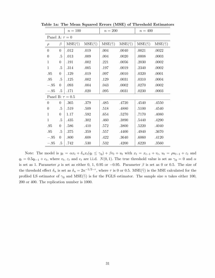
Table 1a: The Mean Squared Errors (MSE) of Threshold Estimators

n = 100 n = 200 n = 400

Panel A: � = 0

� � MSE(b ) MSE(e ) MSE(b ) MSE(e ) MSE(b ) MSE(e )0 0 :012 :019 :004 :0040 :0021 :0022

0 :5 :013 :009 :004 :0020 :0008 :0003

1 0 :191 :002 :221 :0056 :2030 :0002

1 :5 :314 :005 :197 :0019 :2340 :0002

:95 0 :129 :019 :097 :0010 :0320 :0001

:95 :5 :125 :002 :129 :0031 :0310 :0004

�:95 0 :093 :004 :043 :0002 :0270 :0002

�:95 :5 :171 :020 :095 :0031 :0230 :0003

Panel B: � = 0:5

0 0 :365 :379 :485 :4720 :4540 :4550

0 :5 :519 :509 :518 :4880 :5100 :4540

1 0 1:17 :592 :654 :5270 :7170 :4080

1 :5 :435 :302 :460 :3890 :5440 :4290

:95 0 :586 :410 :572 :3800 :5220 :4040

:95 :5 :375 :359 :557 :4400 :4940 :3670

�:95 0 :800 :608 :422 :3640 :6060 :4120

�:95 :5 :742 :530 :532 :4200 :6220 :3560

Note: The model is yt = �xt + �nxt(qt � 0) + �vt + ut with xt = xt�1 + vt, ut = �ut�1 + "t and

qt = 0:5qt�1 + et; where vt, "t and et are i.i.d. N(0; 1): The true threshold value is set as 0 = 0 and �

is set as 1: Parameter � is set as either 0; 1; 0:95 or �0:95. Parameter � is set as 0 or 0:5. The size ofthe threshold e¤ect �n is set as �n = 2n�1=2�� , where � is 0 or 0:5. MSE(b ) is the MSE calculated for thepro�led LS estimator of 0 and MSE(e ) is for the FGLS estimator. The sample size n takes either 100,200 or 400. The replication number is 1000.

31

Table 1b: The Mean Squared Errors of Coe¢ cients Estimators

n = 100 n = 200 n = 400

Panel A: � = 0

� � MSE(b�) MSE(e�) MSE(b�) MSE(e�) MSE(b�) MSE(e�)0 0 3:70e�3 4:50e�3 8:40e�4 9:3e�4 2:13e�4 2:10e�4

0 :5 5:90e�3 5:50e�3 1:14e�3 8:40e�4 2:60e�4 2:13e�4

1 0 1:34 2:60e�1 1:25 1:40e�1 1:27 6:80e�2

1 :5 1:39 2:10e�1 9:80e�1 1:30e�1 9:97e�1 9:10e�2

:95 0 1:66e�1 4:68e�2 3:80e�2 1:70e�2 1:70e�2 5:70e�3

:95 :5 1:81e�1 4:57e�2 4:10e�2 1:60e�2 1:50e�2 5:90e�3

�:95 0 3:50e�2 1:34e�3 2:43e�3 3:50e�4 1:29e�3 9:80e�5

�:95 :5 4:20e�2 1:70e�3 1:93e�3 4:98e�4 1:89e�3 1:08e�4

Panel B: � = 0:5

0 0 1:36e�2 1:44e�2 3:19e�3 3:49e�3 6:89e�4 1:00e�3

0 :5 1:60e�2 1:44e�2 4:20e�3 3:70e�3 1:13e�3 9:50e�4

1 0 1:88 2:01e�1 1:09 1:05e�1 9:62e�1 6:15e�2

1 :5 1:66 2:10e�1 1:50 1:41e�1 9:80e�1 6:56e�2

:95 0 1:81e�1 4:89e�2 7:50e�2 2:14e�2 2:11e�2 6:30e�3

:95 :5 2:40e�1 5:29e�2 9:50e�2 1:81e�2 2:48e�2 5:93e�3

�:95 0 1:40e�1 5:70e�3 3:22e�2 1:59e�3 5:90e�3 2:66e�4

�:95 :5 1:06e�1 5:20e�3 2:25e�2 1:43e�3 7:40e�3 1:16e�4


qt = 0:5qt�1 + et; where vt, "t and et are i.i.d. N(0; 1): The true threshold value is set as 0 = 0 and � is

set as 1: Parameter � is set as either 0; 1; 0:95 or �0:95. Parameter � is set as 0 or 0:5. The size of thethreshold e¤ect �n is set as �n = 2n�1=2�� , where � is 0 or 0:5. MSE(b�) is de�ned as the sum of MSE(b�)and MSE(b�n); where MSE(b�) is the MSE calculated for the pro�led LS estimator of � and MSE(b�n) isMSE calculated for the pro�led LS estimator of �: MSE(e�) is de�ned as the sum of MSE(e�) and MSE(e�n);where MSE(e�) is the MSE for the FGLS estimator of � and MSE(e�n) is for the FGLS estimator of �n: Thesample size n takes either 100, 200 or 400. The replication number is 1000.

32

Table 2a: Size Performancen = 100 n = 200 n = 400

� �n � 10% 5% 1% 10% 5% 1% 10% 5% 1%

Panel A: Tn0 0 0 :078 :028 :005 :114 :056 :018 :098 :046 :008

0 0 :5 :120 :092 :034 :084 :050 :008 :076 :052 :010

1 0 0 :132 :082 :030 :064 :034 :014 :068 :044 :013

1 0 :5 :086 :052 :022 :134 :074 :022 :112 :076 :018

:95 0 0 :128 :073 :042 :178 :072 :030 :104 :046 :008

:95 0 :5 :134 :075 :020 :146 :064 :004 :132 :061 :016

�:95 0 0 :120 :072 :010 :106 :060 :018 :093 :042 :015

�:95 0 :5 :070 :034 :008 :118 :064 :006 :092 :039 :006

Panel B: eTn0 0 0 :110 :072 :030 :102 :062 :022 :098 :047 :010

0 0 :5 :144 :084 :028 :076 :044 :014 :088 :046 :008

1 0 0 :084 :058 :020 :112 :038 :018 :104 :054 :014

1 0 :5 :130 :062 :014 :082 :042 :014 :116 :055 :012

:95 0 0 :114 :062 :002 :072 :060 :008 :082 :042 :008

:95 0 :5 :128 :064 :032 :132 :076 :020 :094 :037 :008

�:95 0 0 :086 :036 :016 :142 :078 :024 :090 :044 :010

�:95 0 :5 :116 :066 :022 :089 :046 :016 :091 :058 :015


qt = 0:5qt�1 + et; where vt, "t and et are i.i.d. N(0; 1): The true threshold value is set as 0 = 0 and � is

set as 1: Parameter � is set as either 0; 1; 0:95 or �0:95. Parameter � is set as 0 or 0:5. The size of thethreshold e¤ect �n is set as 0 to check the size performance. n is the sample size. The replication number

is 1000.

33

Table 2b: Power Performancen = 100 Tn eTnPanel A: � = 0

� � 10% 5% 1% > (ln(n))2 10% 5% 1% > (ln(n))2

0 0 1:00 :994 :984 :956 1:00 :998 :988 :970

0 :5 :992 :980 :968 :904 :998 :994 :984 :952

1 0 :478 :436 :360 :462 :998 :996 :982 :958

1 :5 :506 :460 :312 :486 1:00 :998 :992 :970

:95 0 :796 :720 :564 :610 :986 :986 :968 :968

:95 :5 :830 :772 :654 :636 :996 :996 :994 :978

�:95 0 :956 :922 :884 :464 1:00 :998 :994 :994

�:95 :5 :856 :802 :708 :444 1:00 1:00 :998 :996

Panel B: � = 0:5

0 0 :322 :224 :074 :024 :324 :206 :110 :034

0 :5 :258 :150 :030 :020 :206 :090 :030 :032

1 0 :164 :098 :050 :100 :278 :190 :078 :044

1 :5 :090 :043 :010 :030 :298 :240 :100 :048

:95 0 :070 :034 :010 :018 :296 :206 :118 :068

:95 :5 :322 :234 :072 :024 :268 :196 :084 :072

�:95 0 :296 :236 :146 :002 :550 :434 :182 :110

�:95 :5 :308 :198 :050 :004 :500 :392 :266 :088



is set as 1: Parameter � is set as either 0; 1; 0:95 or �0:95. Parameter � is set as 0 or 0:5. The size ofthe threshold e¤ect �n is set as �n = 2n�1=2�� , where � is 0 or 0:5. n is the sample size. The replication

number is 1000.

34

Table 2c: Power Performancen = 200 Tn eTnPanel A: � = 0

� � 10% 5% 1% > (ln(n))2 10% 5% 1% > (ln(n))2

0 0 1:00 1:00 :998 :982 1:00 1:00 :998 :984

0 :5 1:00 1:00 :996 :974 1:00 1:00 1:00 :990

1 0 :854 :836 :816 :328 1:00 1:00 1:00 :992

1 :5 :668 :614 :540 :346 1:00 1:00 1:00 :988

:95 0 :856 :820 :732 :624 1:00 1:00 1:00 :986

:95 :5 :790 :750 :708 :584 1:00 1:00 1:00 :992

�:95 0 :962 :950 :912 :506 1:00 1:00 1:00 1:00

�:95 :5 :964 :956 :906 :502 1:00 1:00 1:00 1:00

Panel B: � = 0:5

0 0 :284 :222 :098 :004 :256 :198 :108 :004

0 :5 :254 :144 :078 :002 :250 :170 :066 :008

1 0 :098 :050 :016 :000 :280 :212 :126 :080

1 :5 :116 :050 :010 :030 :292 :174 :072 :014

:95 0 :082 :034 :016 :000 :428 :336 :194 :020

:95 :5 :078 :044 :002 :034 :308 :228 :068 :016

�:95 0 :318 :220 :124 :000 :442 :352 :268 :034

�:95 :5 :110 :050 :016 :000 :402 :292 :160 :030




number is 1000.

35

Table 2d: Power Performancen = 400 Tn eTnPanel A: � = 0

� � 10% 5% 1% > (ln(n))2 10% 5% 1% > (ln(n))2

0 0 1:00 1:00 1:00 1:00 1:00 1:00 1:00 1:00

0 :5 1:00 1:00 1:00 :994 1:00 1:00 1:00 :998

1 0 :742 :692 :586 :234 1:00 1:00 1:00 1:00

1 :5 :546 :488 :410 :266 1:00 1:00 1:00 :998

:95 0 :910 :884 :820 :722 1:00 1:00 1:00 1:00

:95 :5 :942 :916 :868 :668 1:00 1:00 1:00 :998

�:95 0 :994 :986 :958 :596 1:00 1:00 1:00 1:00

�:95 :5 :996 :984 :958 :648 1:00 1:00 1:00 1:00

Panel B: � = 0:5

0 0 :294 :196 :042 :002 :264 :166 :052 :000

0 :5 :166 :124 :054 :000 :272 :192 :108 :002

1 0 :386 :312 :160 :000 :248 :162 :052 :000

1 :5 :020 :012 :002 :012 :228 :146 :050 :002

:95 0 :074 :026 :004 :002 :264 :186 :068 :002

:95 :5 :094 :052 :010 :000 :292 :210 :082 :000

�:95 0 :092 :042 :020 :000 :546 :448 :302 :010

�:95 :5 :134 :064 :018 :000 :320 :204 :134 :010




number is 1000.

36

SFB 649 Discussion Paper Series 2013

For a complete list of Discussion Papers published by the SFB 649, please visit http://sfb649.wiwi.hu-berlin.de. 001 "Functional Data Analysis of Generalized Quantile Regressions" by

Mengmeng Guo, Lhan Zhou, Jianhua Z. Huang and Wolfgang Karl Härdle, January 2013.

002 "Statistical properties and stability of ratings in a subset of US firms" by Alexander B. Matthies, January 2013.

003 "Empirical Research on Corporate Credit-Ratings: A Literature Review" by Alexander B. Matthies, January 2013.

004 "Preference for Randomization: Empirical and Experimental Evidence" by Nadja Dwenger, Dorothea Kübler and Georg Weizsäcker, January 2013.

005 "Pricing Rainfall Derivatives at the CME" by Brenda López Cabrera, Martin Odening and Matthias Ritter, January 2013.

006 "Inference for Multi-Dimensional High-Frequency Data: Equivalence of Methods, Central Limit Theorems, and an Application to Conditional Independence Testing" by Markus Bibinger and Per A. Mykland, January 2013.

007 "Crossing Network versus Dealer Market: Unique Equilibrium in the Allocation of Order Flow" by Jutta Dönges, Frank Heinemann and Tijmen R. Daniëls, January 2013.

008 "Forecasting systemic impact in financial networks" by Nikolaus Hautsch, Julia Schaumburg and Melanie Schienle, January 2013.

009 "‘I'll do it by myself as I knew it all along’: On the failure of hindsight-biased principals to delegate optimally" by David Danz, Frank Hüber, Dorothea Kübler, Lydia Mechtenberg and Julia Schmid, January 2013.

010 "Composite Quantile Regression for the Single-Index Model" by Yan Fan, Wolfgang Karl Härdle, Weining Wang and Lixing Zhu, February 2013.

011 "The Real Consequences of Financial Stress" by Stefan Mittnik and Willi Semmler, February 2013.

012 "Are There Bubbles in the Sterling-dollar Exchange Rate? New Evidence from Sequential ADF Tests" by Timo Bettendorf and Wenjuan Chen, February 2013.

013 "A Transfer Mechanism for a Monetary Union" by Philipp Engler and Simon Voigts, March 2013.

014 "Do High-Frequency Data Improve High-Dimensional Portfolio Allocations?" by Nikolaus Hautsch, Lada M. Kyj and Peter Malec, March 2013.

015 "Cyclical Variation in Labor Hours and Productivity Using the ATUS" by Michael C. Burda, Daniel S. Hamermesh and Jay Stewart, March 2013.

016 "Quantitative forward guidance and the predictability of monetary policy – A wavelet based jump detection approach –" by Lars Winkelmann, April 2013.

017 "Estimating the Quadratic Covariation Matrix from Noisy Observations: Local Method of Moments and Efficiency" by Markus Bibinger, Nikolaus Hautsch, Peter Malec and Markus Reiss, April 2013.

018 "Fair re-valuation of wine as an investment" by Fabian Y.R.P. Bocart and Christian M. Hafner, April 2013.

019 "The European Debt Crisis: How did we get into this mess? How can we get out of it?" by Michael C. Burda, April 2013.

SFB 649, Spandauer Straße 1, D-10178 Berlin http://sfb649.wiwi.hu-berlin.de

This research was supported by the Deutsche

Forschungsgemeinschaft through the SFB 649 "Economic Risk".

SFB 649, Spandauer Straße 1, D-10178 Berlin http://sfb649.wiwi.hu-berlin.de

This research was supported by the Deutsche

Forschungsgemeinschaft through the SFB 649 "Economic Risk".

SFB 649 Discussion Paper Series 2013

For a complete list of Discussion Papers published by the SFB 649, please visit http://sfb649.wiwi.hu-berlin.de. 020 "Disaster Risk in a New Keynesian Model" by Maren Brede, April 2013. 021 "Econometrics of co-jumps in high-frequency data with noise" by Markus

Bibinger and Lars Winkelmann, May 2013. 022 "Decomposing Risk in Dynamic Stochastic General Equilibrium" by Hong

Lan and Alexander Meyer-Gohde, May 2013. 023 "Reference Dependent Preferences and the EPK Puzzle" by Maria Grith,

Wolfgang Karl Härdle and Volker Krätschmer, May 2013. 024 "Pruning in Perturbation DSGE Models - Guidance from Nonlinear Moving

Average Approximations" by Hong Lan and Alexander Meyer-Gohde, May 2013.

025 "The ‘Celtic Crisis’: Guarantees, transparency, and systemic liquidity risk" by Philipp König, Kartik Anand and Frank Heinemann, May 2013.

026 "State Price Densities implied from weather derivatives" by Wolfgang Karl Härdle, Brenda López-Cabrera and Huei-Wen Teng, May 2013.

027 "Bank Lending Relationships and the Use of Performance-Sensitive Debt" by Tim R. Adam and Daniel Streitz, May 2013.

028 "Analysis of Deviance in Generalized Partial Linear Models" by Wolfgang Karl Härdle and Li-Shan Huang, May 2013.

029 "Estimating the quadratic covariation of an asynchronously observed semimartingale with jumps" by Markus Bibinger and Mathias Vetter, May 2013.

030 "Can expert knowledge compensate for data scarcity in crop insurance pricing?" by Zhiwei Shen, Martin Odening and Ostap Okhrin, May 2013.

031 "Comparison of Methods for Constructing Joint Confidence Bands for Impulse Response Functions" by Helmut Lütkepohl, Anna Staszewska-Bystrova and Peter Winker, May 2013.

032 "CDO Surfaces Dynamics" by Barbara Choroś-Tomczyk, Wolfgang Karl Härdle and Ostap Okhrin, July 2013.

033 "Estimation and Inference for Varying-coefficient Models with Nonstationary Regressors using Penalized Splines" by Haiqiang Chen, Ying Fang and Yingxing Li, July 2013.

034 "Robust Estimation and Inference for Threshold Models with Integrated Regressors" by Haiqiang Chen, July 2013.

I L R E Robust Estimation and B Inference for Threshold...

Documents

Transcript of I L R E Robust Estimation and B Inference for Threshold...