SFB 649 Discussion Paper 2016-021

CRIX an Index for blockchain

based Currencies

Simon Trimborn* Wolfgang Karl Härdle*

* Humboldt-Universität zu Berlin, Germany

This research was supported by the Deutsche Forschungsgemeinschaft through the SFB 649 "Economic Risk".

http://sfb649.wiwi.hu-berlin.de

ISSN 1860-5664

SFB 649, Humboldt-Universität zu Berlin Spandauer Straße 1, D-10178 Berlin

SFB

6

4 9

E

C O

N O

M I

C

R I

S K

B

E R

L I

N

CRIX an Index for blockchain basedcurrencies 1

Simon Trimborn 2

Wolfgang Karl Härdle 3

November 3, 2016

The S&P500 or DAX30 are important benchmarks for the financial industry. These andother indices describe different compositions of certain segments of the financial markets.For currency markets, the IMF offers the index SDR. Prior to the Euro, the ECU existed,which was an index representing the development of European currencies. It is surprising,though, to see that the common index providers have not mapped emerging e-coins into anindex yet because with cryptos like Bitcoin, a new kind of asset of great public interest hasarisen. Index providers decide on a fixed number of index constituents which will representthe market segment. It is a huge challenge to set this fixed number and develop the rulesto find the constituents, especially since markets change and this has to be taken intoaccount. A method relying on the AIC is proposed to quickly react to market changes andtherefore enable us to create an index, referred to as CRIX, for the cryptocurrency market.The codes used to obtain the results in this paper are available via www.quantlet.de .

JEL classification: C51, C52, G10

Keywords: Index construction, model selection, AIC, bitcoin, cryptocurrency, CRIX

1Financial support from the Deutsche Forschungsgemeinschaft via CRC 649 ”Economic Risk” and IRTG1792 ”High Dimensional Non Stationary Time Series”, Humboldt-Universität zu Berlin, is gratefullyacknowledged.

2Humboldt-Universität zu Berlin, C.A.S.E. - Center for Applied Statistics and Economics, SpandauerStr. 1, 10178 Berlin, Germany, tel: +49 (0)30 2093-5728, fax: +49 (0)30 2093-5649, E-Mail:simon.trimborn@wiwi.hu-berlin.de

3Humboldt-Universität zu Berlin, C.A.S.E. - Center for Applied Statistics and Economics, SpandauerStr. 1, 10178 Berlin, Germany and SKBI School of Business, Singapore Management University, 50Stamford Road, Singapore 178899, tel: +49 (0)30 2093-5630, E-Mail: haerdle@hu-berlin.de

1 Introduction

More and more companies have started offering digital payment systems. Smartphoneshave evolved into a digital wallet, telephone companies offer banking related services: clearsignal that we are about to enter the era of digital finance. In fact we are already actinginside a digital economy. The market for e-x (x = “finance,” “money,” “book,” you nameit . . . ) has not only picked up enormous momentum but has become standard for drivinginnovative activities in the global economy. A few clicks at y and payment at z brings ourpurchase to location w. Own-currencies for the digital market were therefore just a matterof time. The idea of the Nobel Laureate Hayek, see Hayek (1990), of letting companies offerconcurrent currencies seemed for a long time scarcely probable, but the invention of theBlockchain has made it possible to bring his vision to life. Cryptocurrencies (abbr. cryptos)have surfaced and opened up an angle towards this new level of economic interaction.Since the appearance of bitcoins, several new cryptos have spread through the Web andoffered new ways of proliferation. Even states accept them as legal payment method orpart of economic interaction. E.g., the USA classifies cryptocurrencies as commodities,Kawa (2015), and lately Japan announced that they accept them as a legal currency,EconoTimes (2016). Obviously, the crypto market is fanning out and shows clear signs ofacceptance and deepening liquidity, so that a closer look at its general moves and dynamicsis called for.

The technical aspects behind cryptocurrencies have been reviewed by several researchers.For a well written technical survey, we refer to Tschorsch and Scheuermann (2015). Thetransaction graph of Bitcoin, the Blockchain, has received much attention too, see e.g.Ron and Shamir (2013) and Reid and Harrigan (2013). Even the economics of the Bitcoinhas been studied, e.g. Kristoufek (2014). To our knowledge, the development of theentire cryptocurrency market has not been studied so far, only subsamples have beentaken into account. Elendner et al. (2016) studied the top 10 cryptocurrencies by marketcapitalization and found that their returns are weakly correlated which each other. Thisbrings us to the conclusion that Bitcoin, even though it dominates the market in terms of itsmarket capitalization, does not lead the market. The movements of other cryptocurrenciesare important too, when one analyzes the market of cryptocurrencies. We contribute tothis area of research by designing CRIX, a market index (benchmark) which will enableeach interested party to study the performance of the crypto market as a whole or singlecryptos. Studying the stochastic dynamics of CRIX will allow to create ETFs or contingentclaims.First, the term benchmark has to be defined:

Definition 1. A benchmark is a measure which consists of a selection of cryptos that arerepresenting the market.

Index providers construct their indices in terms of Definition 1 with a fixed number ofconstituents, see e.g. FTSE (2016), S&P (2014) and Deutsche Boerse AG (2013). Butmarkets change which should cause the chosen number of index constituents to be alteredtoo. While trying to mimic the movements of an innovative market like the crypto market,one is confronted with a frequently changing market structure. This calls for a dynamicstructure of the benchmark, especially for the number of constituents. The StrataQuantindex family, see NYSE (2015), for example alters the number of constituents in eachsector index dependent on their affiliation with a certain sector and membership in theRussell1000 index. But the benchmark for the crypto market would not have a parent index

2

since it is meant to be the leading index. Therefore a different approach is necessary thatenables to react to changes in the market structure. A dynamic methodology guaranteeingthe diversity of an index at any time is to be constructed. Furthermore, the benchmark ismeant to be investable. Regarding the portfolio choice, we define the following selectiondefinition:

Definition 2. Between investment portfolios with equal performance, the one with theleast assets is preferable.

This definition corresponds to Occam’s Razor. Following definitions 1 and 2, for thecrypto market CRIX: a CRyptocurrency IndeX, hu.berlin/crix has been established. Tocompute CRIX, we evaluate the differences in the log returns of the market against aselection of possible benchmarks. We figure out, that the AIC works well to evaluate thedifferences. It penalizes the index for the number of constituents, so definitions 1 and 2are met. For the calculation of the respective likelihoods, a non-parametric approach usingthe Epanechnikov (1969) kernel is applied. We proof the impact of the value of an assetin the market on the AIC method, thus we are applying a top-down approach to selectthe assets for the benchmarks to choose from. The number of constituents is recalculatedquarterly to ensure an up-to-date fit to the current market situation. With CRIX one maystudy the contingent claims and the stochastic nature of this index, Chen et al. (2016), orstudy the crypto market characteristics against traditional markets, Härdle and Trimborn(2015).

This paper is structured as follows. Section 2 introduces the topic and reviews thebasics of index construction. In Section 3 the method for dynamic index constructionis described and Section 4 introduces the remaining rules for CRIX. Section 5 describesfurther variants to create a CRIX family. Their performance is tested in Section 6. InSections 7 and 8 the new method is applied to the German and Mexican stock markets tocheck the performance of the methodology against existing indices. The codes used toobtain the results in this paper are available via www.quantlet.de.

2 Index construction

The basic idea of any price index is to weight the prices of its constituent goods by thequantities of the goods purchased or consumed. The Laspeyres index takes the value of abasket of k assets and compares it against a base period:

PL0t(k) =

∑ki=1 PitQi0∑ki=1 Pi0Qi0

(1)

with Pit the price of asset i at time t and Qi0 the quantity of asset i at time 0 (the baseperiod). For market indices, such as CRSP, S&P500 or DAX, the quantity Qi0 is thenumber of shares of the asset i in the base period. Multiplied with its corresponding price,the market capitalization results, hence the constituents of the index are weighted bytheir market capitalizations. But markets change. A company which was representativefor market developments yesterday might no longer be important today. On top of that,companies can go bankrupt, a corporation can raise the number of its outstanding shares,or trading in it can become infrequent. All these situations must produce a change in theindex structure, so that the market is still adequately represented. Hence companies haveto drop out of the index and have to be replaced by others. The index rules determine in

3

which cases such an event happens. The formula of Laspeyres (1) can not handle suchevents entirely because a change of constituents will result in a change in the index valuethat is not due to price changes. Therefore, established price indices like DAX or S&P500,see Deutsche Boerse AG (2013) and S&P (2014) respectively, and the newly founded indexCRIX(k), a CRyptocurrency IndeX, hu.berlin/crix, use the adjusted formula of Laspeyres,

CRIXt(k, β) =∑ki=1 βi,t−

lPitQi,t−

l

Divisor(k)t−l

(2)

with P , Q and i defined as before, βi,t−lthe adjustment factor of asset i found at time

point t−l , l indicates that this is the l-th adjustment factor, and t−l the last time pointwhen Qi,t−

l, Divisor(k)i,t−

land βi,t−

lwere updated. In the classical setting, βi,t−

lis defined

to be βi,t−l

= 1 for all i and l. Anyhow, some indices use βi,t−lto achieve maximal weighting

rules, e.g. Deutsche Boerse AG (2013) and MEXBOL (2013). The Divisor ensures thatthe index value of CRIX has a predefined value on the starting date. It is defined as

Divisor(k, β)0 =∑ki=1 βi0Pi0Qi0

starting value . (3)

The starting value could be any possible number, commonly 100, 1000 or 10000. It ensuresthat a positive or negative development from the base period will be revealed. Wheneverchanges to the structure of CRIX occur, the Divisor is adjusted in such a way that onlyprice changes are reflected by the index. Defining k1 and k2 as number of constituents, itresults∑k1

i=1 βi,t−l−1Pi,t−1Qi,t−

l−1

Divisor(k1, β)t−l−1

= CRIXt−1(k1, β) = CRIXt(k2, β) =∑k2j=1 βi,t−

lPj,tQj,t−

l

Divisor(k2, β)t−l

. (4)

In indices like FTSE, S&P500 or DAX the number of index members is fixed, k1 = k2,see FTSE (2016), S&P (2014) and Deutsche Boerse AG (2013). As long as the goalbehind these indices is the reflection of the price development of the selected assets, thisis a straightforward approach. But, e.g., DAX is also meant to be an indicator for thedevelopment of the market as a whole, see Janßen and Rudolph (1992). This raisesautomatically the question of whether the included assets are representing the market.Since the constituents are chosen using a top-down approach, meaning that the biggestcompanies by market capitalization are included, the intuitive answer is yes. But it leavesa sour taste that additional assets may describe the market more appropriately. One mayobject by referring to total market indices like the Wilshire 5000, S&P Total Market Indexor CRSP U.S. Total Market Index, see Wilshire Associates (2015), S&P (2015) and CRSP(2015), that are providing a full description. But financial praxis has shown that smallerindices like DAX30 and S&P500 receive more attention in evaluating the movements oftheir corresponding markets. It is therefore appealing to know which are the representativeassets in a market and which smaller number of index constituents eases the handling of atracking portfolio. Additionally, one may be concerned that an index would include illiquidand non-investable assets which makes the management of a tracking portfolio even moredifficult. Figure 1 shows that this is indeed a problem in the crypto-currencies market.Some cryptos have a fairly high market capitalization while their respective trading volumeis very low. An asset which is not frequently traded can not add enough information to a

4

●

●

●

●

●

●

●●●●●● ●

●

●

●●●

●●

●●

●

●

●

●●

●

●●

●

●●

●●●●

●●●

●●

●●

●

●

●

●

●●●

●

●

●●●●●

●

●●

●

●

●

●

●

●

●●●●●

●●

●●●

●

●

●●

●

●

●

● ●●●

●

●●

●●

●●

● ●●

●

●●● ●●

●

●

●

●●

●

●

●

●●

●

●

●●●●●

●

●

●●●

●●

●

●●

●

●

●

●●●

●

●●

●

●

●

●●

●●●●

●

●●●●

●●●

●

●●●

●

●●●

●

●

●●

●

●●

●

●●

●

●●

●●

●

●

●●●

●

●●●

●

●

● ●

●

●● ●

●●

●

● ●

●

●

●

●●●

●●

●●

●●●● ●●

●

●●

●●

●

●●

●

●●

●

●

●

●●●

●●

●●

●

●

●

● ●●

● ●

●

●

●

●

●●

●●

●

●●

●●●

●●

●

●

●●

●

●●●

●

●●

●

●

●●

●

●

●

●●●

●

●

●●

●

●●

●●

●

●

●

●●●

●

●

●

●

●

●

●

●●

●

● ●

●

●

●●

●●

●

●

●

●

●

5 10 15 20

−10

010

20

Comparison volume and market capitalization

log mean market capitalization

log

mea

n vo

lum

e

Figure 1: Comparison of the log mean trading volume and log mean market capitalization,both measured in USD, for all cryptos in the dataset over the time period20140401 - 20160807

VolMarketCapComparison

market index to display market changes and is difficult to trade for an investor.These thoughts raise the question which value of k is "optimal" for building an investable

benchmark for the market. Additionally, especially young and innovative markets maychange their structure over time. Therefore, a quantification of an accurate cryptobenchmark with sparse number of constituents is asked for. Since the crypto market showsa frequently changing market structure with a huge number of illiquid cryptos, we apply atime varying index selection structure.

3 Dynamic index construction

This section is dedicated to describing the composition rule which is used to find thenumber of index members—the spine of CRIX. Since CRIX will be a benchmark for thecrypto market, the dimension and evaluation of the market has to be defined:

Definition 3. The total market (TM) consists of all cryptos in the crypto universe. Itsvalue is the combined market value of the cryptos.

To compare the TM with a benchmark candidate, it will be normalized by a Divisor,

TM(K)t =∑Ki=1 PitQi,t−

l

Divisor(K)t−l

(5)

with K the number of all cryptos in the crypto universe. Note that no adjustment factoris used for TM(K)t. Further define the log returns:

5

ε(K)TMt = log{TM(K)t} − log{TM(K)t−1} (6)ε(k, β)CRIXt = log{CRIX(k, β)t} − log{CRIX(k, β)t−1}, (7)

where CRIX(k, β)t is the CRIX with k constituents at time point t.The goal is to optimize k and β so that a sparse but accurate approximation in terms of

mink,β‖ε(k, β)‖2 = ‖ε(K)TM − ε(k, β)CRIX‖2, (8)

is achieved. We chose a squared loss function in (8), since it heavily penalizes deviations.The expected squared loss is defined as

E(‖ε(k, β)‖2) =∫ ∞−∞‖ε(k, β)‖2

2f{ε(k, β)}dε(k, β) (9)

The density, f , is estimated nonparametrically with an Epanechnikov kernel, sinceaccording to Härdle et al. (2004) the Epanechnikov (1969) kernel shows a good balancebetween variance optimization and numerical performance. In nonparametric estimationwith an Epanechnikov kernel, Epa, the estimator of f is derived by

f̂h(x) = 1nh

n∑i=1

Epa(x− xih

), Epa(u) = 34(1− u2)I(|u| ≤ 1)

where h is the bandwidth.The bandwidth selection is performed with the plug-in selector by Sheather and Jones

(1991) and further described in Wand and Jones (1994). The plug-in selector is derivedunder the loss function Mean Integrated Squared Error, MISE. Hall (1987) found that theKullback-Leibler (KL) loss function for selecting the smoothing parameter of the kerneldensity is highly influenced by the tails of the distribution. Devroye and Györfi (1985)mention that Mean Integrated Error (MIE) is stronger affected than MISE by the tailsof the distribution and Kanazawa (1993) claims that MIE shall be used if interest is inmodeling the tails. Kanazawa (1993) investigates that the use of a Kullback-Leibler lossfunction would put more weight on the tails compared to MISE. Since this is not in ourinterest, the choice of the density smoothing parameter, h, is performed under MISE. Asalready mentioned, the AIC will be used later to choose the index.

Since the value of TM(K)t is unknown and not measurable due to a lack of information,the total market index will be defined and used as a proxy for the TM(K). The definitionis inspired by total market indices like CRSP (2015), S&P (2015) and Wilshire Associates(2015). They use all stocks for which prices are available.

Definition 4. The total market index (TMI) contains all cryptos in the crypto universefor which prices are available. The cryptos are weighted by their market capitalization.

This changes (5) to

TMIt(kmax) =∑kmaxi=1 PitQi,t−

l

Divisor(kmax)t−l

6

with kmax the maximum number of cryptos with available prices and (8) to

mink,β‖ε̂(k, β)‖2 = ‖ε(kmax)TM − ε(k, β)CRIX‖2 (10)

s.t.: 1 ≤ k ≤ ku

ku ∈ [1, kmax]s ∈ [1, kmax − k]

β1×(k+s) = (1, . . . , 1, βk+1, . . . , βk+s)>

βk+1, . . . , βk+s ∈ (−∞,∞).

We introduced several constraints with (10). We will search for an index under theclassical approach of Laspeyres, where β = 1. We include βk+1, . . . , βk+s to evaluateif adding s more assets to the index explains the difference between ε(kmax)TM andε(k, β)CRIX better. The first k assets won’t be adjusted by a parameter, so no parameterestimation is necessary. This makes the first term a constant. The parameters of the nexts assets have to be estimated.A number of criteria are applicable. In this context: cross validation (CV), full cross

validation (FCV), Generalized Cross Validation (GCV), Generalized Full Cross Validation(GFCV), Mallows’ Cp, Akaike’s Final Prediction Error (FPE), Shibata (SH), AIC, BICand Hannan Quinn (HQ), Droge (2006). The first one, CV, see Stone (1974), is a widelyused criterion

CV(k, β) = T−1T∑i=1{ε(kmax)TMt − ε(k, β)CRIX−t }2 (11)

where ε(k, β)CRIX−t is the estimate of ε(k, β)CRIXt without the observation t. It is howevernot suitable as FCV in this context because CV does not involve any penalty for thenumber of constituents, Bunke et al. (1999). The GCV criterion, see Craven and Wahba(1978), is defined as

GCV{ε̂(k, β), s} = T−1∑Tt=1 ε̂(k, β)2

t

(1− T−1s)2 (12)

by assuming that s < T . One shall note that s and not k + s defines the number ofvariables to penalize for, since k parameters are set to be 1 and need not be estimated.According to Arlot and Celisse (2010), the asymptotic optimality of GCV was shown inseveral frameworks. The GFCV, see Droge (1996):

GFCV{ε̂(k, β), s} = T−1T∑t=1

ε̂(k, β)2t (1 + T−1s)2 (13)

is an alteration.A further score, SH,

SH{ε̂(k, β), s} = T + 2sT 2

T∑t=1

ε̂(k, β)2t , (14)

was shown to be asymptotically optimal, Shibata (1981), and asymptotically equivalent toMallows’ Cp, FPE and AIC.

7

Mallows (1973)’ Cp:

Cp{ε̂(k, β), s} =∑Tt=1 ε̂(k, β)2

t

σ̂(k, β)2 − T + 2 · s (15)

with σ̂(k, β)2 the variance of ε̂(k, β). Cp{ε̂(k, β), s} tends to choose models which overfitand is not consistent in selecting the true model, see Mallick and Yi (2013), Woodroofe(1982) and Nishii (1984).

The FPE uses the formula

FPE{ε̂(k, β), s} = T + s

(T − s)T

T∑t=1

ε̂(k, β)2t , (16)

see Akaike (1970). So far, the discussed criteria depend on little data information. Just thesquared residuals and, in the case of Mallows’ Cp, the variance are taken into account. Thefurther criteria use more information by depending on the maximum likelihood, derived by

L{ε̂(k, β)} = maxβ

∏t

f{ε̂(k, β)t}, (17)

where f , in (9), represents the density of the ε̂(k, β)t over all t. The first one is the AICwhich is defined to be

AIC{ε̂(k, β), s} = −2 logL{ε̂(k, β)}+ s · 2, (18)

Akaike (1998). If the true model is of finite dimension, then neither FPE nor AIC areconsistent, compare Hurvich and Tsai (1989). But Shibata (1983) showed the asymptoticefficiency of Mallows’ Cp, FPE and AIC under the assumption of an infinite number ofregression variables or an increasing number of regression variables with the sample size.On the other hand, the BIC, defined as

BIC{ε̂(k, β), s} = −2 logL{ε̂(k, β)}+ s · log(T ), (19)

see Schwarz (1978), is consistent in choosing the true model, Nishii (1984). A furtherconsistent criterion is the one proposed by Hannan and Quinn (1979), defined as

HQ{ε̂(k, β), s} = −2 logL{ε̂(k, β)}+ 2s · log{log(T )}. (20)

We’ll evaluate now which criteria to use for our purpose. Since CRIX is to be a benchmarkmodel, all possible models under certain restrictions for the number of parameters areincluded in the test set, ΘAIC = {CRIX(k1, β),CRIX(k2, β), . . . }, where k1, k2, . . . arepredefined values. Recall that the intention behind CRIX is to discover the best model todescribe the data (benchmark) under a squared loss function.Define the loss function in (9) for ε̂(k, β),

RT{ε̂(k, β)} = E(||ε̂(k, β)||2), (21)

and define the number of constituents which minimize the risk in RT (k, β) as k∗ and s∗for the model set Θ, Shibata (1983). For this paragraph, consider ε̂(k, β) ∼ N(0, σ̂(k, β)2).k∗ and s∗ will be interpreted as the number of constituents which balance the bias and

8

variance, defineHT{ε̂(k, β), s} = ||ε̂(k, β)||2 + sσ̂(k, β)2. (22)

Mean efficiency shall be defined as

eff(Θ) = HT (ε̂(k∗, β), s∗)/RT (Θ). (23)

A criteria is defined to be asymptotic mean efficient if

a.eff(Θ) = lim infT→∞

HT{ε̂(k∗, β), s∗}/RT (Θ) = 1 (24)

This result holds if the number of constituents , k∗ and s∗, increases with T , Shibata (1983).Of course, this result was derived under the assumption of normally distributed errors.Since we are estimating the distribution non parametrically, this result might not hold.For example, Boisbunon et al. (2013) investigate that the result for gaussian distributederrors should hold for spherically symmetric and elliptically contoured distributions too.This leads us to the conclusion that asymptotic optimality might be still given in this case.We oracle so, because for infinitely many observations, the nonparametric estimator tendsto the true distribution, Härdle et al. (2004).

The assumption of k∗ and s∗ increasing with T is plausible in this case since longer timehorizons T would include cryptos which aren’t part of shorter ones due to bankruptcy orsince they haven’t been found yet. Both lead to more complexity. It follows that all ofthe asymptotically optimal criteria would lead to a mean efficient model choice in termsof squared risk for a given selection of models which fits the intention to discover a bestmodel. It remains to find the suitable one.Define the characteristic function as

ϕ(t) =∫ ∞−∞

exp(itx)f(x)dx (25)

with i ∈ C and t ∈ R. The Fourier inversion theorem states (Shephard (1991)):

Theorem 1. Suppose g and ϕ are integrable in the Lebesgue sense and

ϕ(t) =∫ ∞−∞

exp(itx)g(x)dx, (26)

theng(x) = 1

2π

∫ ∞−∞

exp(−itx)ϕ(t)dt. (27)

holds everywhere.

The moment generating function is defined as

M(t) =∫ ∞−∞

exp(tx)f(x)dx. (28)

If the moments generating function exists, it holds

ϕ(t) = M(it). (29)

We see that the characteristic function depends on the moment generating function of ε̂.Most of the asymptotically optimal criteria depend on the empirical versions of the first

9

two moments of ε̂. Just the AIC uses the full distribution via the likelihood and thereforeall the moments. This makes its information basis richer. For the derivation of the numberof index members of CRIX, we will use the AIC, because it uses the most informationcompared to the other asymptotically optimal criteria: it is the only one which dependson the likelihood.To decide with AIC which number k should be used, a procedure was created which

compares the squared difference between log returns of the TMI, see Definition 4, andseveral candidate indices,

‖ε̂(kj, β)‖2 = ‖ε(kmax)TM − ε(kj, β)CRIX‖2, (30)

where ε(kj, β)CRIX is the log return of CRIX version with kj constituents and ε̂(kj, β)is the respective difference. The candidate indices, CRIX(kj, β), have different numbersof constituents which fulfill k1 < k2 < k3 < · · · , where kj = k1 + s(̇j − 1). Therefore,the number of constituents between the indices are equally spaced. By definition bothinformation criteria evaluate the differences, ε̂(kj, β), between the candidates and the TMIwith the respective likelihood L{ε̂(kj, β), s}, see Equations (18) and (19). This procedureimplies that the IC method evaluates if s more assets add information to CRIX. If so,these assets are added to the intercept and the next s assets are tested for. We expectassets with a higher market capitalization to have a higher influence on the AIC, so weformulated the following theorem:Theorem 2. The rate of improvement of the AIC depends on the relative value of anasset in the market.

The proof for the Theorem 2 is given in the Appendix, 10.1, under the assumption ofnormally distributed error terms. Therefore, we will follow the common practise to includethe assets with the highest market capitalization in the index, see e.g. Deutsche Boerse AG(2013) or MEXBOL (2013),

arg maxi

k∑j=1

Pj,i,t−lQj,i,t−

l, i ∈ {1, . . . , K}. (31)

Thus, we apply a top-down approach to decide about the number of index constituents.For the sorting of the index constituents by highest market capitalization, we just rely

on the closing data of the last day of a month. We chose to do so, since the next periodsCRIX will just depend on Qi,t−

l, (2), and not on data which lie further in the past. This is

in line with the methodology of e.g. the DAX.Since the differences between the TMI(kmax) and CRIX(kj, β) are caused over time by

the missing time series in CRIX(kj, β), the independence assumption of the ε̂(kj, β) for allj can not be fulfilled by construction. But Györfi et al. (1989) give arguments that undercertain conditions, the rate of convergence is essentially the same as for an independentsample. Since the same data are used to estimate f j and the information criterion, a“leave-one-out” cross-validation procedure is performed in order to have in-sample data forthe calculation of the density and pseudo-out-of-sample data for the information criterion,hence new observations; see Boisbunon et al. (2013). Summarizing the described procedure,results to:

1. At time point T + 1, construct TMI(kmax)

2. Set j = 1

10

3. Construct CRIX(kj, 1) and CRIX(kj, β), j = 1, 2, 3, . . . , k1 < k2 < k3 < · · ·

4. Compute ε̂(kj, β) and ε̂(kj, 1)

5. Kernel density estimation for density f j(ε̂(kj, β)) and f j(ε̂(kj, 1)) with leave-one-outcross validationa) Perform for ε̂(kj, β) and ε̂(kj, 1), where ε̂ belongs to the respective return series:b) Construct T datasets ε̂−t = {. . . , ε̂t−1, ε̂t+1, . . . }, leaving out ε̂t.c) Compute the Kernel Density Estimator (KDE) for each ε̂−t.d) Compute the log likelihood (18) for ε̂t with KDE for ε̂−t.e) Sum the log likelihoods

6. Derive AIC{ε̂(kj, β), s} and AIC{ε̂(kj, 1), 0}

7. If j = (kmax − s): stop, else jump to 3. and j = j + 1

The next section describes the further index rules for CRIX.

4 CRIX family rules

The constituents of the indices are regularly checked so that the corresponding indexalways represents its asset universe well. It is common to do this on a quarterly basis, seee.g. Deutsche Boerse AG (2013), MEXBOL (2013) and S&P (2014). In case of CRIX thisreallocation is much faster. In the past, coins have shown a very volatile behavior, not justin the manner of price volatility. In some weeks, many occur out of nothing in the marketand many others vanish from the market even when they were before very important,e.g., Auroracoin. This calls for a faster reallocation of the market benchmark than on aquarterly basis. We choose a monthly reallocation to make sure that CRIX catches themomentum of the cryptocurrency market well. Therefore, on the last day of every month,the cryptos which had the highest market capitalization on the last day in the last monthwill be checked and the first k will be included in CRIX for the coming month.

Since a review of an index is commonly performed on a quarterly basis the number ofindex members of CRIX will be checked on a quarterly basis too. The described procedurefrom Section 3 will be applied to the observations from the last three months on the lastday of the third month after the markets closed. The number of index constituents, k,will be used for the next three months. Thus, CRIX corresponds to a monthly rebalancedportfolio which number of constituents is reviewed quarterly.It may happen that some data are missing for some of the analyzed time series. If an

isolated missing value occurs alone in the dataset, meaning that the values before andafter it are not missing, then Missing At Random (MAR) is assumed. This assumptionmeans that just observed information cause the missingness, Horton and Kleinman (2007).The Last-Observation-Carried-Forward (LOCF) method is then applied to fill the gap forthe application of the AIC. We did not choose a different approach since a regression orimputation may alter the data in the wrong direction. By LOCF, we imply no changeand just do not exclude the crypto. If two or more data are missing in a row, then theMAR assumption may be violated, therefore no method is applied. The correspondingtime series is then excluded from the computation in the derivation period. If data aremissing during the computation of the index values, the LOCF method is applied too.

11

This is done to make the index insensitive to this crypto at this time point. CRIX shouldmimic market changes, therefore an imputation or regression method for the missing datawould distort the view of the market.

Before we continue, we summarize the rules which were described so far:

• Quarterly altering of the number of index constituents

• Monthly altering of the index constituents

• AIC used for model selection

• Nonparametric estimation of the density

• Application of a top-down approach to select the assets for the subset analysis

• Application of LOCF if trading of an asset stops before next reallocation

5 The CRIX family

Using the described methods and rules from above, three indices will be proposed. Thisindices provide a different look at the market.

1. CRIX:The first and leading index is CRIX. While the choice for the best number ofconstituents is made, their numbers are chosen in steps of five. It is common inpractice to construct market indices with a number of constituents which is evenlydivisible by five, see e.g. FTSE (2016), S&P (2014), Deutsche Boerse AG (2013).Therefore this choosing is performed for CRIX(k), k = 5, 10, 15, . . . . Since the globalminimum for the AIC criterion may involve many index constituents, but a sparseindex is the goal, the search for the optimal model terminates at level j whenever

AIC{ε̂(kj, β), 5} < AIC{ε̂(kj, 1), 0}. (32)

Therefore merely a local optimum will be achieved in most of the cases for Θ = ΘAIC ,in (23). But the choice is still asymptotically optimal by defining Θ = {ΘAIC |ki ≤kj∀i}. In Section 6 it will be shown that the performance of the index is alreadyvery good.

2. ECRIX:The second constructed index is called Exact CRIX (ECRIX). It follows the aboverules too. But the number of its constituents is chosen in steps of 1. Therefore theset of models contains CRIX(k), k = 1, 2, 3, . . . and stops when

AIC{ε̂(kj, β), 1} < AIC{ε̂(kj, 1), 0}. (33)

3. EFCRIX:Since the decision procedures for CRIX and ECRIX terminate when the AIC risesfor the first time, Exact Full CRIX will be constructed to visualize whether thedecision procedure works fine for the two covered indices. The intention is to have anindex which may approach the TMI but only in case even small assets help improve

12

Aug 01 2014 Dec 01 2014 Apr 01 2015 Aug 01 2015 Dec 01 2015 Apr 01 2016 Aug 01 2016

400

600

800

1000

1200

1400

Performance of CRIX with AIC

Date

Inde

x va

lue

Figure 2: Performance of CRIXCRIXindex CRIXcode

the view of the total market, a benchmark for the benchmarks. It’ll be derived withthe AIC procedure, compare Section 3. The decision rule is based on

minkj ,β

AIC{ε̂(kj, β), 1} (34)

for Θ = ΘAIC , in (23). This index computes the AIC for every possible number ofconstituents and what is chosen is the number where the AIC becomes minimal.

6 Performance analysis

The indices CRIX, ECRIX, EFCRIX have been proposed to give insight into the cryptomarket. Our RDC crypto database covers data for 331 cryptocurrencies, kindly providedby CoinGecko. The data used for the analysis cover daily closing data for prices, marketvolume and market capitalization in USD for each crypto in the time period from 2014-04-01 to 2016-08-06. Crypto exchanges are open on the weekends, therefore data for weekendclosing prices exist. Since crypto exchanges do not finish trading after a certain time pointevery day, a time point which serves as a closing time has to be defined. CoinGecko used12 am UTC time zone. One should note that missing data are observed in the dataset,therefore the last rules from Chapter 4 will come into play.

Figure 2 shows the performance of CRIX, and Figure 3 the differences between CRIX andboth ECRIX and EFCRIX. For the purpose of comparison, the indices were recalibratedon the recalculation dates since the index constituents change then. We do not provideeach index plot individually since they perform almost equally. However, the AIC methodgave very different numbers of constituents for the corresponding indices. The numbers ofconstituents are given in Table 3. For comparison, we provide the number of constituentsunder the other discussed model selection criteria too. The variance of Cp was derivedwith a GARCH(1,1) model, Bollerslev (1986). The corresponding information for ECRIXand EFCRIX are given in the same Table, 3. Apparently the methodology of EFCRIX

13

causes its number of constituents to become close to maximal in every period. ECRIX hasmostly much fewer constituents than CRIX and EFCRIX due to the fact that this indexjust runs until a local optimum. Comparing the number of constituents for CRIX derivedwith AIC against the other criteria, one sees that GCV, GFCV and SH tend to choosemore or the same number of constituents than AIC. Also all three criteria suggest thesame result. FPE results in much more constituents than any other criteria for CRIX andECRIX. Cp stops at the initial value for CRIX and ECRIX, just for EFCRIX it differs.For CRIX, ECRIX and EFCRIX, AIC chooses less constituents compared to all othercriteria, except Cp which terminates very early.

AIC GCV GFCV SH Cp FPECRIX 18.4500 3.4049 3.4049 3.4049 25.7485 0.0312ECRIX 444.2490 386.8260 386.8260 386.8260 768.4531 0.0324EFCRIX 0.0314 0.0324 0.0324 0.0324 165.9407 0.0324

Table 1: Comparison of CRIX, ECRIX, EFCRIX, derived under different penalizations,against TMI under Mean Squared Error

AIC GCV GFCV SH Cp FPECRIX 0.9891 0.9946 0.9946 0.9946 0.9864 1.0000ECRIX 0.9511 0.9592 0.9592 0.9592 0.9117 1.0000EFCRIX 1.0000 1.0000 1.0000 1.0000 0.9728 1.0000

Table 2: Comparison of CRIX, ECRIX, EFCRIX, derived under different penalizations,against TMI under Mean Directional Accuracy

Since the indices CRIX and ECRIX are just optimized until a local optimum, they areexpected to perform less optimal than the EFCRIX against the TMI. Table 1 gives theMean Square Error (MSE) and Table 2 the Mean Directional Accuracy (MDA), defined as

MSE{CRIX(k)} = 1T

T∑t=1{CRIX(k)t − TMI(kmax)t}2 (35)

MDA{CRIX(k)} = 1T

T∑t=1

I[sign{TMI(kmax)t − TMI(kmax)t−1}

= sign{CRIX(k)t − CRIX(k)t−1}] (36)

where I(·) is the indicator function and sign(·) gives the sign of the respective equation.The recalibration of the indices on the recalculation date is important for the computationof the MSE, since altering the constituents may change the future development in termsof MSE. The MDA is insensitive to the recalibration. Apparently EFCRIX performs best,which can be explained due to its larger number of index constituents. The CRIX, ECRIXand EFCRIX are close in terms of the MDA but the MSE is much better for EFCRIX.Additionally, ECRIX performs worse than CRIX in terms of MSE and MDA. Comparingall the model selection criteria, we see that FPE has the best performance in terms ofMSE and MDA. This is not surprising since this criteria selected the most constituents.The more important risk criteria is the MDA, since the direction of the TMI shall beadequately modeled by the criteria. Table 2 shows that the AIC either performs second

14

worst or performs equally good to the other criteria. But the MDA is close to the one ofthe outperforming ones. The reason for the lower value is the lower number of constituents.Interestingly, AIC outperforms in terms of MSE and MDA for EFCRIX, which choses theglobal optimum.

CRIX was constructed with steps of five which is common in practice, but this analysisshowed that ECRIX would work well for the crypto market too. Additionally, the analysisshowed that it is indeed unnecessary to choose the global optimal AIC. Even a localoptimum and a much lower number of constituents is able to mimic the market movementsvery well in terms of the MDA. Furthermore, even for ECRIX there was more than oneconstituent selected most of the time. This shows that Bitcoin, which currently clearlydominates the market in terms of market capitalization and trading volume, doesn’t leadthe market. Other cryptocurrencies are important for the market movements too.We are aware that the AIC didn’t outperform the other criteria in terms of MDA and

MSE for the local optimum. But for the global optimum, AIC outperforms while havingsometimes less constituents. We conclude that the AIC works best in search of the globaloptimum, but for the local optimum we observed a diverging picture. But the AIC stillperformed very well. Due to the theoretical choice for the AIC and its global optimalbehavior, we continue working with the AIC.

CRIX ECRIX EFCRIXAIC GCV GFCV SH Cp FPE AIC GCV GFCV SH Cp FPE AIC GCV GFCV SH Cp FPE

1 10 10 10 10 5 40 1 4 4 4 1 41 41 41 41 41 1 412 30 30 30 30 5 115 5 14 14 14 1 117 98 117 117 117 4 1173 30 30 30 30 5 160 4 4 4 4 1 162 161 162 162 162 1 1624 5 45 45 45 5 190 3 3 3 3 1 192 187 192 192 192 14 1925 15 15 15 15 5 205 1 6 6 6 1 208 206 208 208 208 1 2086 20 35 35 35 5 215 6 16 16 16 1 215 215 215 215 215 20 2157 5 5 5 5 5 220 1 1 1 1 1 221 220 221 221 221 10 2218 15 65 65 65 5 170 3 3 3 3 1 167 153 167 167 167 5 1679 5 5 5 5 5 220 2 5 5 5 1 223 219 223 223 223 3 223

Table 3: Comparison of AIC, GCV, GFCV, SH, Cp and the FPE method for the selectionof the number of index constituents for the CRIX, ECRIX and EFCRIX in the 9periods

7 Application to the German stock market

The CRIX methodology was derived with the idea of finding a method which allowsmimicking young and fast changing markets appropriately. But well known major marketsusually change their structure too. We tested the proposed methodology on the Germanstock market, which has four major indices: DAX, MDAX, SDAX and TecDAX. The DAXis used to determine the overall market direction, Janßen and Rudolph (1992). Since it ischosen from the so called prime segment, it has some prior restrictions. It is interestingto see whether our methodology yields the DAX as an adequate benchmark for the totalmarket. Following Definition 4, we define all available stocks as the TMI and apply ournew method to find an appropriate index. Again, the 7-step method from Section 3 wasapplied to find the number of constituents, but it starts at 30 members to check if moreconstituents are necessary. The method for the identification of k and the reallocationof the included assets is performed quarterly, like DAX. To be in line with the DAX

15

Aug 01 2014 Dec 01 2014 Apr 01 2015 Aug 01 2015 Dec 01 2015 Apr 01 2016 Aug 01 2016

−10

0−

500

Differences between Indices derived with AIC and TMI

Date

Diff

eren

ce b

etw

een

Indi

ces

and

TM

I

Figure 3: Realized difference between TMI and CRIX (solid), ECRIX (dashed), EFCRIX(dotdashed)

CRIXfamdiff CRIXcode

reallocation dates, the index calculation will start after the third Friday of September andthe reallocation dates are the third Fridays of December, March, June and September, seeDeutsche Boerse AG (2013).The data were fetched from Datastream in the period 20000616 until 20151218. We

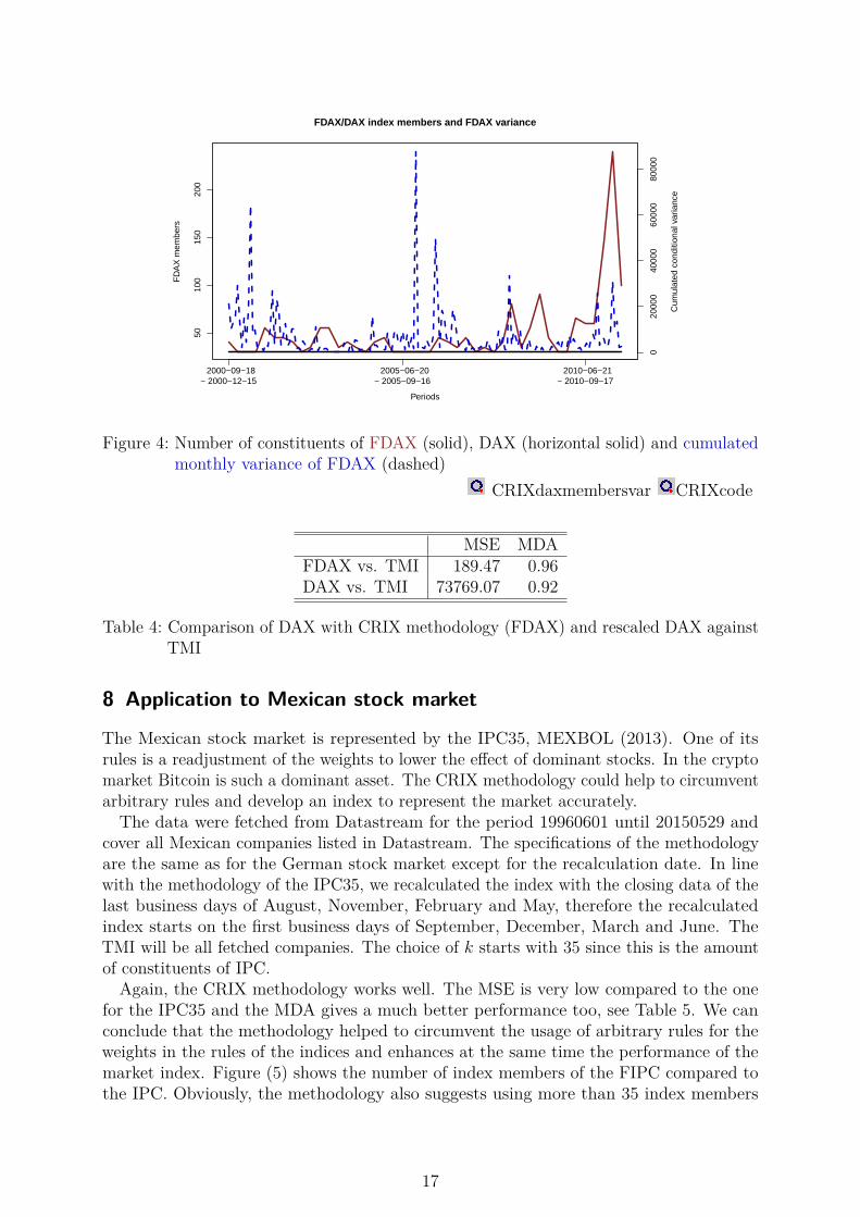
took all stocks which are German companies and are traded on XETRA. Any time seriesfor which Datastream reported an error either for the price or market capitalization datawas excluded from the analysis. The index, computed with the new methodology, is calledFlexible DAX (FDAX). One should note that the analysis starts three months after thestarting point of the dataset due to the initialization period of FDAX.Figure 4 shows the number of members of FDAX and DAX in the respective periods.

Most of the time, the number of index constituents for FDAX is higher than the 30members of DAX. Just around 2004-2005 is the k more frequently 30. Especially whilethe turmoil of the financial markets, starting from 2008/2009, is the number of indexconstituents much higher. One might hint that a higher reported variability in one periodshould cause an increase in k in the next period, since it was shown that the selectionmethod depends on the variance, see Section 10. Figure 4 shows that this idea canpartially be supported. The derivation of the conditional variance was performed with aGARCH(1,1) model, Bollerslev (1986), and the daily results were summed up. Obviously,in the extreme cases increases the k in the next period, see 2001, 2006 and 2011.The computation of the MSE and MDA, see Table 4, shows that FDAX is a more

accurate benchmark for the total market as DAX. Since Janßen and Rudolph (1992) statethat DAX may be used to analyze the movements of the total market, an MDA of 92 % isindeed good. But FDAX mimics the market even better, with an MDA of 96 %. Also theMSE for FDAX is much lower than the one of DAX. Therefore the methodology fulfilledits goal to find a sparse, investable and accurate benchmark, depending on the MDA.

16

5010

015

020

0

FDAX/DAX index members and FDAX variance

Periods

FD

AX

mem

bers

2000−09−18 − 2000−12−15

2005−06−20 − 2005−09−16

2010−06−21 − 2010−09−17

020

000

4000

060

000

8000

0

Cum

ulat

ed c

ondi

tiona

l var

ianc

e

Figure 4: Number of constituents of FDAX (solid), DAX (horizontal solid) and cumulatedmonthly variance of FDAX (dashed)

CRIXdaxmembersvar CRIXcode

MSE MDAFDAX vs. TMI 189.47 0.96DAX vs. TMI 73769.07 0.92

Table 4: Comparison of DAX with CRIX methodology (FDAX) and rescaled DAX againstTMI

8 Application to Mexican stock market

The Mexican stock market is represented by the IPC35, MEXBOL (2013). One of itsrules is a readjustment of the weights to lower the effect of dominant stocks. In the cryptomarket Bitcoin is such a dominant asset. The CRIX methodology could help to circumventarbitrary rules and develop an index to represent the market accurately.The data were fetched from Datastream for the period 19960601 until 20150529 and

cover all Mexican companies listed in Datastream. The specifications of the methodologyare the same as for the German stock market except for the recalculation date. In linewith the methodology of the IPC35, we recalculated the index with the closing data of thelast business days of August, November, February and May, therefore the recalculatedindex starts on the first business days of September, December, March and June. TheTMI will be all fetched companies. The choice of k starts with 35 since this is the amountof constituents of IPC.Again, the CRIX methodology works well. The MSE is very low compared to the one

for the IPC35 and the MDA gives a much better performance too, see Table 5. We canconclude that the methodology helped to circumvent the usage of arbitrary rules for theweights in the rules of the indices and enhances at the same time the performance of themarket index. Figure (5) shows the number of index members of the FIPC compared tothe IPC. Obviously, the methodology also suggests using more than 35 index members

17

4060

8010

0

Comparison of IPC and FIPC index members

Periods

FIP

C/IP

C m

embe

rs

1996−09−02 − 1996−12−02

2001−06−01 − 2001−09−03

2006−06−01 − 2006−09−01

Figure 5: Number of constituents of FIPC (solid) and IPC (dashed) in the respectiveperiods

CRIXipcmembers CRIXcode

most of the time which is the number of members of the IPC.

MSE MDAFIPC vs. TMI 319.25 0.97IPC vs. TMI 27177417.58 0.91

Table 5: Comparison of IPC with CRIX methodology (FIPC) and rescaled IPC againstTMI

18

9 Conclusion

The movements of cryptocurrencies are very different from each other, Elendner et al.(2016). So studying the entire market of cryptocurrencies requires an instrument whichadequately captures and displays the market movements, an index. But index constructionfor cryptocurrencies requires a new methodology to find the right number of index members.Innovative markets, like the one for cryptocurrency’s, change their structure frequently.The proposed methods were applied to oracle a new family of indices, which are displayedand updated on a daily basis on hu.berlin/crix. The performance of the new indiceswere studied and it was shown that the dynamic AIC based methodology results in indiceswith stable properties. The results show that a market like the crypto market - momentarilydominated by Bitcoin - still needs a representative index since Bitcoin does not lead themarket. The AIC based method was also applied to the German stock market. The resultsyield a more accurate benchmark in terms of MDA. In applying the CRIX methodologyto the Mexican stock market, which is dominated by Telmex, one finds high accuracy of itin terms of MSE and MDA.We conclude, that the CRIX technology enhances the construction of an index if the

goal is to find a sparse, investable and accurate benchmark.

19

References

Akaike, H. (1998). “Information Theory and an Extension of the Maximum LikelihoodPrinciple”. Selected Papers of Hirotugu Akaike. Ed. by E. Parzen, K. Tanabe, and G.Kitagawa. Springer Series in Statistics. Springer New York, pp. 199–213.

Akaike, H. (1970). “Statistical predictor identification”. Annals of the Institute of StatisticalMathematics 22.1, pp. 203–217.

Arlot, S. and A. Celisse (2010). “A survey of cross-validation procedures for model selection”.Statistics Surveys 4, pp. 40–79.

Boisbunon, A., S. Canu, D. Fourdrinier, W. Strawderman, and M. T. Wells (2013). “AIC,Cp and estimators of loss for elliptically symmetric distributions”. arXiv:1308.2766[math, stat].

Bollerslev, T. (1986). “Generalized autoregressive conditional heteroskedasticity”. Journalof Econometrics 31.3, pp. 307–327.

Bunke, O., B. Droge, and J. Polzehl (1999). “Model Selection, Transformations andVariance Estimation in Nonlinear Regression”. Statistics 33, pp. 197–240.

Chen, S., C. Y.-H. Chen, W. K. Härdle, T. M. Lee, and B. Ong (2016). “A first econometricanalysis of the CRIX family”. SFB 649 Discussion Paper forthcoming in Digital Bankingand Internet Finance.

Craven, P. and G. Wahba (1978). “Smoothing noisy data with spline functions”. NumerischeMathematik 31.4, pp. 377–403.

CRSP (2015). “CRSP U.S. Equity Indexes Methodology Guide”. crsp.com/.

Deutsche Boerse AG (2013). “Guide to the Equity Indizes of Deutsche Boerse”. www.dax-indices.com.

Devroye, L. and L. Györfi (1985). Nonparametric Density Estimation The L1 View. Wiley.

Droge, B. (1996). “Some Comments on Cross-Validation”. Statistical Theory and Compu-tational Aspects of Smoothing. Ed. by W. K. Härdle and M. G. Schimek. Contributionsto Statistics. Physica-Verlag HD, pp. 178–199.

Droge, B. (2006). “Asymptotic properties of model selection procedures in linear regression”.Statistics 40.1, pp. 1–38.

EconoTimes (2016). “Japans Cabinet Approves New Bitcoin Regulations”. econotimes.com.

Elendner, H., S. Trimborn, B. Ong, and T. M. Lee (2016). “The Cross-Section of Crypto-Currencies as Financial Assets: An Overview”. SFB 649 Discussion Paper forthcomingin Digital Banking and Internet Finance.

Epanechnikov, V. (1969). “Non-Parametric Estimation of a Multivariate ProbabilityDensity”. Theory of Probability & Its Applications 14.1, pp. 153–158.

20

FTSE (2016). “FTSE UK Index Series”. www.ftse.com.

Györfi, L., W. K. Härdle, P. Sarda, and P. Vieu (1989). Nonparametric Curve Estimationfrom Time Series. Ed. by L. Györfi, W. K. Härdle, P. Sarda, and P. Vieu. Lecture Notesin Statistics 60. Springer New York.

Hall, P. (1987). “On Kullback-Leibler Loss and Density Estimation”. The Annals ofStatistics 15.4, pp. 1491–1519.

Hannan, E. J. and B. G. Quinn (1979). “The Determination of the Order of an Au-toregression”. Journal of the Royal Statistical Society. Series B (Methodological) 41.2,pp. 190–195.

Härdle, W. K., M. Müller, S. Sperlich, and A. Werwatz (2004). Nonparametric andSemiparametric Models. Springer Science & Business Media.

Härdle, W. K. and S. Trimborn (2015). “CRIX or evaluating Blockchain based currencies”.Oberwolfach Report No. 42/2015 “The Mathematics and Statistics of Quantitative Risk”.

Hayek, F. A. (1990). Denationalization of Money: An Analysis of the Theory and Practiceof Concurrent Currencies. 3. Edition. London: Institute of Economic Affairs.

Horton, N. J. and K. P. Kleinman (2007). “Much ado about nothing: A comparison ofmissing data methods and software to fit incomplete data regression models”. TheAmerican Statistician 61.1, pp. 79–90.

Hurvich, C. M. and C.-L. Tsai (1989). “Regression and time series model selection in smallsamples”. Biometrika 76.2, pp. 297–307.

Janßen, B. and B. Rudolph (1992). “Der Deutsche Aktienindex DAX”. Fritz Knapp Verlag.

Kanazawa, Y. (1993). “Hellinger distance and Kullback—Leibler loss for the kernel densityestimator”. Statistics & Probability Letters 18.4, pp. 315–321.

Kawa, L. (2015). “Bitcoin Is Officially a Commodity, According to U.S. Regulator”.Bloomberg.com.

Kristoufek, L. (2014). “What are the main drivers of the Bitcoin price? Evidence fromwavelet coherence analysis”. arXiv:1406.0268 [physics, q-fin].

Mallick, H. and N. Yi (2013). “Bayesian Methods for High Dimensional Linear Models”.Journal of Biometrics & Biostatistics 1.

Mallows, C. L. (1973). “Some Comments on Cp”. Technometrics 15.4, pp. 661–675.

MEXBOL (2013). “Prices and Quotations Index (MEXBOL) - Methodology Note”.bmv.com.

Nishii, R. (1984). “Asymptotic Properties of Criteria for Selection of Variables in MultipleRegression”. The Annals of Statistics 12.2, pp. 758–765.

21

NYSE (2015). “StrataQuant Index Family”. www.nyse.com.

Potapov, A., J. R. Muirhead, S. R. Lele, and M. A. Lewis (2011). “Stochastic gravitymodels for modeling lake invasions”. Ecological Modelling 222.4, pp. 964–972.

Reid, F. and M. Harrigan (2013). “An Analysis of Anonymity in the Bitcoin System”.Security and Privacy in Social Networks. Ed. by Y. Altshuler, Y. Elovici, A. B. Cremers,N. Aharony, and A. Pentland. Springer New York, pp. 197–223.

Ron, D. and A. Shamir (2013). “Quantitative Analysis of the Full Bitcoin TransactionGraph”. Financial Cryptography and Data Security. Ed. by A.-R. Sadeghi. Lecture Notesin Computer Science 7859. Springer Berlin Heidelberg, pp. 6–24.

Schwarz, G. (1978). “Estimating the Dimension of a Model”. The Annals of Statistics 6.2,pp. 461–464.

Sheather, S. J. and M. C. Jones (1991). “A Reliable Data-Based Bandwidth SelectionMethod for Kernel Density Estimation”. Journal of the Royal Statistical Society. SeriesB. Methodological 53, pp. 683–690.

Shephard, N. G. (1991). “From Characteristic Function to Distribution Function: A SimpleFramework for the Theory”. Econometric Theory 7.4, pp. 519–529.

Shibata, R. (1981). “An Optimal Selection of Regression Variables”. Biometrika 68.1,pp. 45–54.

Shibata, R. (1983). “Asymptotic mean efficiency of a selection of regression variables”.Annals of the Institute of Statistical Mathematics 35.1, pp. 415–423.

S&P (2014). “Index Mathematics - Methodology”. us.spindices.com.

S&P (2015). “Dow Jones Total Stock Market Indices Methodology”. us.spindices.com.

Stone, M. (1974). “Cross-validatory choice and assessment of statistical predictions”.Journal of the Royal Statistical Society. Series B (Methodological), pp. 111–147.

Tschorsch, F. and B. Scheuermann (2015). “Bitcoin and Beyond: A Technical Survey onDecentralized Digital Currencies”. IEEE Communications Surveys Tutorials.

Wand, M. P. and M. C. Jones (1994). “Multivariate plug-in bandwidth selection”. Compu-tational Statistics 9.2, pp. 97–116.

Wilshire Associates (2015). “Wilshire 5000 Total Market Index Methodology”. wilshire.com.

Woodroofe, M. (1982). “On Model Selection and the ARC Sine Laws”. The Annals ofStatistics 10.4, pp. 1182–1194.

22

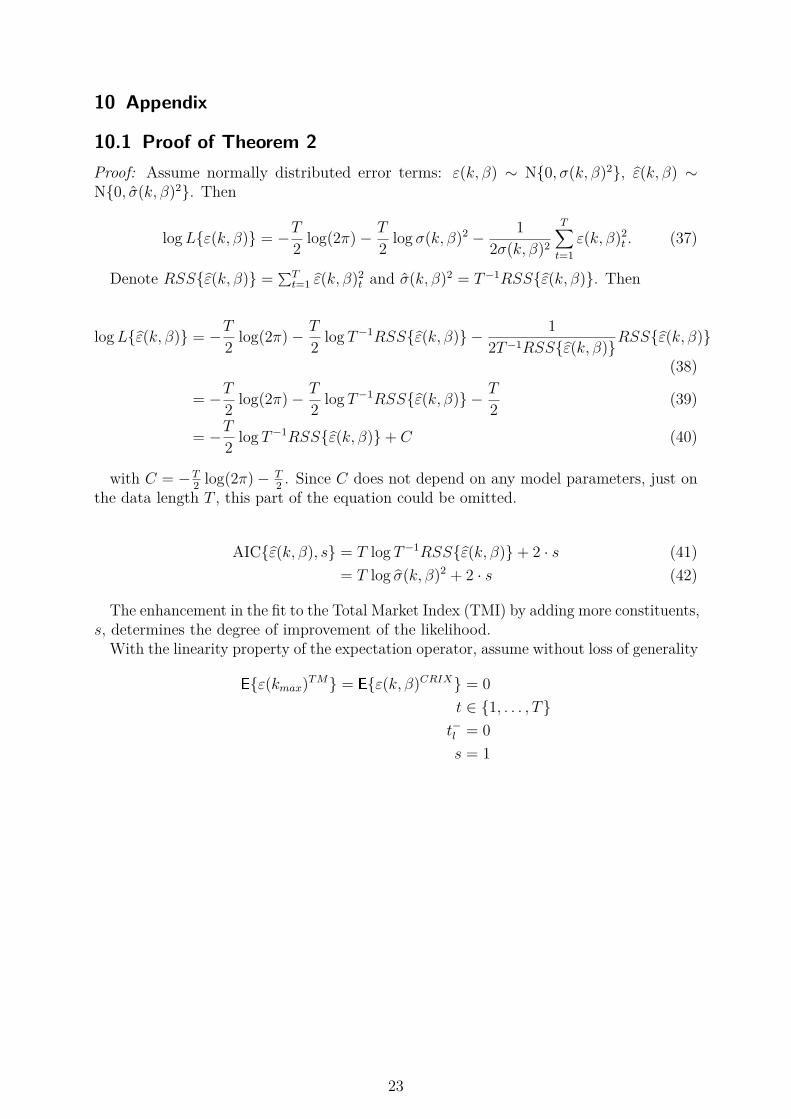
10 Appendix

10.1 Proof of Theorem 2Proof: Assume normally distributed error terms: ε(k, β) ∼ N{0, σ(k, β)2}, ε̂(k, β) ∼N{0, σ̂(k, β)2}. Then

logL{ε(k, β)} = −T2 log(2π)− T

2 log σ(k, β)2 − 12σ(k, β)2

T∑t=1

ε(k, β)2t . (37)

Denote RSS{ε̂(k, β)} = ∑Tt=1 ε̂(k, β)2

t and σ̂(k, β)2 = T−1RSS{ε̂(k, β)}. Then

logL{ε̂(k, β)} = −T2 log(2π)− T

2 log T−1RSS{ε̂(k, β)} − 12T−1RSS{ε̂(k, β)}RSS{ε̂(k, β)}

(38)

= −T2 log(2π)− T

2 log T−1RSS{ε̂(k, β)} − T

2 (39)

= −T2 log T−1RSS{ε̂(k, β)}+ C (40)

with C = −T2 log(2π)− T

2 . Since C does not depend on any model parameters, just onthe data length T , this part of the equation could be omitted.

AIC{ε̂(k, β), s} = T log T−1RSS{ε̂(k, β)}+ 2 · s (41)= T log σ̂(k, β)2 + 2 · s (42)

The enhancement in the fit to the Total Market Index (TMI) by adding more constituents,s, determines the degree of improvement of the likelihood.

With the linearity property of the expectation operator, assume without loss of generality

E{ε(kmax)TM} = E{ε(k, β)CRIX} = 0t ∈ {1, . . . , T}t−l = 0s = 1

23

σ̂(k, β) = Var{ε̂(k, β)}= Var{ε(kmax)TM − ε(k, β)CRIX}

=T∑t=1

[log

kmax∑i=1

PitQi,0(k∑i=1

Pi,t−1Qi,0 + β1Pk+1,t−1Qk+1,0)

− logkmax∑i=1

Pi,t−1Qi,0(k∑i=1

Pi,tQi,0 + β1Pk+1,tQk+1,0)]2

=T∑t=1

[log

kmax∑i=1

PitQi,0

k∑i=1

Pi,t−1Qi,0 +kmax∑i=1

PitQi,0β1Pk+1,t−1Qk+1,0

− log

kmax∑i=1

Pi,t−1Qi,0

k∑i=1

Pi,tQi,0 +kmax∑i=1

Pi,t−1Qi,0β1Pk+1,tQk+1,0

]2

Using the relation log(a+ b) = log(a) + log(1 + b

a), it results:

=T∑t=1

[log

kmax∑i=1

PitQi,0

k∑i=1

Pi,t−1Qi,0

+ log{

1 +∑kmaxi=1 PitQi,0β1Pk+1,t−1Qk+1,0∑kmaxi=1 PitQi,0

∑ki=1 Pi,t−1Qi,0

}

− logkmax∑i=1

Pi,t−1Qi,0

k∑i=1

Pi,tQi,0

+ log{

1 +∑kmaxi=1 Pi,t−1Qi,0β1Pk+1,tQk+1,0∑kmaxi=1 Pi,t−1Qi,0

∑ki=1 Pi,tQi,0

}]2

=T∑t=1

(log

kmax∑i=1

PitQi,0

k∑i=1

Pi,t−1Qi,0

− logkmax∑i=1

Pi,t−1Qi,0

k∑i=1

Pi,tQi,0

+[log

{1 + β1Pk+1,t−1Qk+1,0∑k

i=1 Pi,t−1Qi,0

}− log

{1 + β1Pk+1,tQk+1,0∑k

i=1 Pi,tQi,0

}])2

(43)

Solving the derivation and writing the terms which do not depend on β1 as At and thelast part of (43) as Bt:

σ̂(k, β) =T∑t=1

At + 2 logkmax∑i=1

PitQi,0

k∑i=1

Pi,t−1Qi,0

Bt − 2 logkmax∑i=1

Pi,t−1Qi,0

k∑i=1

Pi,tQi,0

Bt +B2t

=T∑t=1

At + 2Bt

logkmax∑i=1

PitQi,0

k∑i=1

Pi,t−1Qi,0

− logkmax∑i=1

Pi,t−1Qi,0

k∑i=1

Pi,tQi,0

+B2

t

=T∑t=1

At + 2Bt

[ε(kmax)TM − ε(k, 1)CRIX

]+B2

t

Since normally distributed error terms are assumed, note that β1 = Cov{ε̂(k,1),εk+1}V ar{εk+1}

, whereεk+1 is the log return of Pi,tQi,0. We see that the change in the variance will depend onthe additional variance which the new constituent can explain, see β1. Furthermore, itdepends on the value of Pk+1,tQk+1,0 relative to ∑k

i=1 Pi,tQi,0, (43), which is the summedmarket value of the constituents in the index. This infers that constituents with a highermarket capitalization are more likely to be part of the index. �

This gives support to using the often applied top-down approach, which we use for theconstruction of CRIX too.

24

SFB 649 Discussion Paper Series 2016 For a complete list of Discussion Papers published by the SFB 649, please visit http://sfb649.wiwi.hu-berlin.de. 001 "Downside risk and stock returns: An empirical analysis of the long-run

and short-run dynamics from the G-7 Countries" by Cathy Yi-Hsuan Chen, Thomas C. Chiang and Wolfgang Karl Härdle, January 2016.

002 "Uncertainty and Employment Dynamics in the Euro Area and the US" by Aleksei Netsunajev and Katharina Glass, January 2016.

003 "College Admissions with Entrance Exams: Centralized versus Decentralized" by Isa E. Hafalir, Rustamdjan Hakimov, Dorothea Kübler and Morimitsu Kurino, January 2016.

004 "Leveraged ETF options implied volatility paradox: a statistical study" by Wolfgang Karl Härdle, Sergey Nasekin and Zhiwu Hong, February 2016.

005 "The German Labor Market Miracle, 2003 -2015: An Assessment" by Michael C. Burda, February 2016.

006 "What Derives the Bond Portfolio Value-at-Risk: Information Roles of Macroeconomic and Financial Stress Factors" by Anthony H. Tu and Cathy Yi-Hsuan Chen, February 2016.

007 "Budget-neutral fiscal rules targeting inflation differentials" by Maren Brede, February 2016.

008 "Measuring the benefit from reducing income inequality in terms of GDP" by Simon Voigts, February 2016.

009 "Solving DSGE Portfolio Choice Models with Asymmetric Countries" by Grzegorz R. Dlugoszek, February 2016.

010 "No Role for the Hartz Reforms? Demand and Supply Factors in the German Labor Market, 1993-2014" by Michael C. Burda and Stefanie Seele, February 2016.

011 "Cognitive Load Increases Risk Aversion" by Holger Gerhardt, Guido P. Biele, Hauke R. Heekeren, and Harald Uhlig, March 2016.

012 "Neighborhood Effects in Wind Farm Performance: An Econometric Approach" by Matthias Ritter, Simone Pieralli and Martin Odening, March 2016.

013 "The importance of time-varying parameters in new Keynesian models with zero lower bound" by Julien Albertini and Hong Lan, March 2016.

014 "Aggregate Employment, Job Polarization and Inequalities: A Transatlantic Perspective" by Julien Albertini and Jean Olivier Hairault, March 2016.

015 "The Anchoring of Inflation Expectations in the Short and in the Long Run" by Dieter Nautz, Aleksei Netsunajev and Till Strohsal, March 2016.

016 "Irrational Exuberance and Herding in Financial Markets" by Christopher Boortz, March 2016.

017 "Calculating Joint Confidence Bands for Impulse Response Functions using Highest Density Regions" by Helmut Lütkepohl, Anna Staszewska-Bystrova and Peter Winker, March 2016.

018 "Factorisable Sparse Tail Event Curves with Expectiles" by Wolfgang K. Härdle, Chen Huang and Shih-Kang Chao, March 2016.

019 "International dynamics of inflation expectations" by Aleksei Netšunajev and Lars Winkelmann, May 2016.

020 "Academic Ranking Scales in Economics: Prediction and Imdputation" by Alona Zharova, Andrija Mihoci and Wolfgang Karl Härdle, May 2016.

SFB 649, Spandauer Straße 1, D-10178 Berlin http://sfb649.wiwi.hu-berlin.de

This research was supported by the Deutsche

Forschungsgemeinschaft through the SFB 649 "Economic Risk".

SFB 649, Spandauer Straße 1, D-10178 Berlin http://sfb649.wiwi.hu-berlin.de

This research was supported by the Deutsche

Forschungsgemeinschaft through the SFB 649 "Economic Risk".

SFB 649 Discussion Paper Series 2016 For a complete list of Discussion Papers published by the SFB 649, please visit http://sfb649.wiwi.hu-berlin.de. 021 "CRIX an Index for blockchain based currencies" by Simon Trimborn and

Wolfgang Karl Härdle, May 2016.

SFB 649, Spandauer Straße 1, D-10178 Berlin http://sfb649.wiwi.hu-berlin.de

This research was supported by the Deutsche

Forschungsgemeinschaft through the SFB 649 "Economic Risk".

SFB 649, Spandauer Straße 1, D-10178 Berlin http://sfb649.wiwi.hu-berlin.de

This research was supported by the Deutsche

Forschungsgemeinschaft through the SFB 649 "Economic Risk".