I L R A Theory of Price E B Adjustment under Loss Aversion

SFB 649 Discussion Paper 2014-065

A Theory of Price Adjustment under Loss

Aversion

Steffen Ahrens* Inske Pirschel**

Dennis J. Snower***

* Technische Universität Berlin, Germany ** Kiel Institute for the World Economy, Germany

***Christian-Albrechts University, Germany

This research was supported by the Deutsche Forschungsgemeinschaft through the SFB 649 "Economic Risk".

http://sfb649.wiwi.hu-berlin.de

ISSN 1860-5664

SFB 649, Humboldt-Universität zu Berlin Spandauer Straße 1, D-10178 Berlin

SFB

6

4 9

E C

O N

O M

I C

R

I S

K

B

E R

L I

N

A Theory of Price Adjustment under LossAversion∗

Steffen Ahrensa,b, Inske Pirschelb,c, and Dennis J. Snowerb,c,d

a Technische Universität Berlin, Straße des 17. Juni 135, 10623 Berlin, Germanyb Kiel Institute for the World Economy, Kiellinie 66, 24105 Kiel, Germany

c Christian-Albrechts University, Kiel, Wilhem-Seelig-Platz 1, 24118 Kiel, Germanyd CEPR and IZA

October 30, 2014

Abstract

We present a new partial equilibrium theory of price adjustment, based on con-sumer loss aversion. In line with prospect theory, the consumers’ perceived utilitylosses from price increases are weighted more heavily than the perceived utilitygains from price decreases of equal magnitude. Price changes are evaluated rel-ative to an endogenous reference price, which depends on the consumers’ ratio-nal price expectations from the recent past. By implication, demand responsesare more elastic for price increases than for price decreases and thus firms face adownward-sloping demand curve that is kinked at the consumers’ reference price.Firms adjust their prices flexibly in response to variations in this demand curve, inthe context of an otherwise standard dynamic neoclassical model of monopolisticcompetition. The resulting theory of price adjustment is starkly at variance withpast theories. We find that - in line with the empirical evidence - prices are moresluggish upwards than downwards in response to temporary demand shocks, whilethey are more sluggish downwards than upwards in response to permanent demandshocks.

JEL classification: D03, D21, E31, E50.Keywords: price sluggishness, loss aversion, state-dependent pricing

∗This paper is part of the Kiel-INET research group on new economic thinking. We thank the participantsat the 18th Spring Meeting of Young Economists 2013 in Aarhus (Denmark), the 2013 Annual Meeting ofthe German Economic Association in Düsseldorf (Germany), and the Scottish Economic Society AnnualConference 2014 in Perth (Scotland) for fruitful discussions. Steffen Ahrens acknowledges support by theDeutsche Forschungsgemeinschaft (DFG) through the CRC 649 “Economic Risk.”

E-mail: [email protected] (S. Ahrens), [email protected] (I. Pirschel),[email protected] (D.J. Snower).

1

1 IntroductionThis paper presents a theory of price sluggishness based on consumer loss aversion,along the lines of prospect theory (Kahnemann and Tversky, 1979). The theory hasdistinctive implications, which are starkly at variance with major existing theories ofprice adjustment. In particular, the theory implies that prices are more sluggish up-wards than downwards in response to temporary demand shocks, while they are moresluggish downwards than upwards in response to permanent demand shocks.

These implications turn out to be consonant with recent empirical evidence. Thoughthis evidence has not thus far attracted much explicit attention, it is clearly implicit ina range of influential empirical results. For instance, Hall et al. (2000) document thatfirms mostly accommodate negative temporary demand shifts by temporary price cuts,yet they are reluctant to temporarily increase their prices in response to positive tem-porary demand shifts. Furthermore, the empirical evidence provided by Kehoe andMidrigan (2008) indicates that temporary price reductions are - on average - larger andmuch more frequent than temporary price increases, implying that prices are relativelydownward responsive.

By contrast, in the event of a permanent demand shock, the empirical evidencepoints towards a stronger upward flexibility of prices for a wide variety of industrializedcountries (Kandil, 1995, 1996, 1998, 2001, 2002a,b 2010; Weise, 1999; Karras 1996;Karras and Stokes 1999) as well as developing countries (Kandil, 1998).

While current theories of price adjustment (e.g. Taylor, 1979; Rotemberg, 1982;Calvo, 1983; among many others) fail to account for these empirical regularities, thispaper offers a possible theoretical rationale.

The basic idea underlying our theory is simple. Price increases are associated withutility losses for consumers, whereas price decreases are associated with utility gains.In the spirit of prospect theory, losses are weighted more heavily than gains of equalmagnitude. Consequently, demand responses are more elastic to price increases than toprice decreases. The result is a kinked demand curve1, for which the kink depends onthe consumers’ reference price. In the spirit of Koszegi and Rabin (2006), we modelthe reference price as the consumers’ rational price expectations. We assume that con-sumers know, with a one period lag, whether any given demand shock is temporary orpermanent. Permanent shocks induce changes in the consumers’ rational price expec-tations and thereby in their reference price, while temporary shocks do not.

Given the demand shock is temporary, the kink of the demand curve implies thatsufficiently small shocks do not affect the firm’s price. This is the case of price rigidity.For larger shocks, the firm’s price will respond temporarily, but the size of the responsewill be asymmetric for positive and negative shifts of equal magnitude. Since negativeshocks move the firm along the relatively steep portion of the demand curve, pricesdecline stronger to negative shocks than they increase to equiproportionate positiveshocks.

By contrast, given the demand shock is permanent, the firm can foresee not onlythe change in demand following its immediate pricing decision, but also the resultingchange in the consumers’ reference price. A rise in the reference price raises the firms’long-run profits (since the reference price is located at the kink of the demand curve),

1Modeling price sluggishness by means of a kinked demand curve is of course a well-trodden path.Sweezy (1939) and Hall and Hitch (1939) modeled price rigidity in an oligopolistic framework along theselines. In these models, oligopolistic firms do not change their prices flexibly because of their expectedasymmetric competitor’s reactions to their pricing decisions. A game theoretic foundation of such model ispresented by Maskin and Tirole (1988).

2

whereas a fall in the reference price lowers long-run profits, a phenomenon which weterm the reference-price updating effect. On this account, firms are averse to initiatingpermanent price reductions. By implication, prices are more sluggish downwards thanupwards for permanent demand shocks.

These results are extremely important for the conduct of monetary policy, sincethey imply that the sign of the asymmetry of price adjustment depends on the per-sistence of the underlying demand shock. In particular, if temporary demand shocksare interpreted as non-persistent and permanent demand shocks as fully persistent, ouranalysis implies that there exists a balance point (i.e. an intermediate degree of per-sistence of the shock) at which the asymmetry reverses. For shocks less persistentthan the balance point prices are more sluggish upwards than downwards, while theyare more sluggish downwards than upwards for more persistent shocks. Whether thedegree of persistence at the balance point is relatively high or low depends on the ad-justment speed of the reference price and on the firm’s discount factor. An increasein the adjustment speed of the reference price, as well as in the firm’s discount factor,strengthens the role of the reference-price updating effect, increasing upward flexibilityand downward sluggishness at any given positive persistence of the shock. Therefore,the balance point will be associated with a lower level of persistence. To the best ofour knowledge, there is no other paper studying the ramifications of the persistence ofthe demand shock for asymmetric price adjustment.

The paper is structured as follows. Section 2 reviews the relevant literature. Section3 presents our general model setup and in Section 4 we analyze the effects of variousdemand shocks on prices, both analytically and numerically. Section 5 concludes.

2 Relation to the LiteratureWe now consider the empirical evidence suggesting that prices respond imperfectly andasymmetrically to exogenous positive and negative shocks of equal magnitude, and thatthe implied asymmetry depends on whether the shock is permanent or temporary.

There is much empirical evidence for the proposition that, with regard to perma-nent demand shocks, prices are generally more responsive to positive shocks than tonegative ones. For example, in the context of monetary policy shocks, Kandil (1996,2002b), Kandil (1995), and Weise (1999) find support for the United States over a largerange of different samples. Moreover, Kandil (1995) and Karras and Stokes (1999) sup-ply evidence for large panels of industrialized OECD countries, while Karras (1996)provides evidence for developing countries. In the case of the United States, Kandil(2001, 2002a) shows that the asymmetry also prevails in response to permanent gov-ernment spending shocks. Kandil (1999, 2006, 2010), on the other hand, looks directlyat permanent aggregate demand shocks and also confirms the asymmetry for a largeset of industrialized countries as well as for a sample of disaggregated industries inthe United States. Comparing a large set of industrialized and developing countries,Kandil (1998) finds that the asymmetry is even stronger for many developing countriescompared to industrialized ones.

In addition to the asymmetric price reaction in response to permanent demandshocks, the above studies also find an asymmetric reaction of output. They show thatoutput responds significantly less to permanent positive demand shocks relative to neg-ative ones. This asymmetry – which is also predicted by our model (as shown below) –is further documented by a large body of empirical literature that explicitly focuses onoutput. For example, DeLong and Summers (1988), Cover (1992), Thoma (1994), and

3

Ravn and Sola (2004) show for the United States that positive changes in the rate ofmoney growth induce much weaker output reductions than negative changes in the rateof money supply. Morgan (1993) and Ravn and Sola (2004) confirm this asymmetry,when monetary policy is conducted via changes in the federal funds rate. Additionalevidence is provided by Tan et al. (2010) for Indonesia, Malaysia, the Philippines, andThailand and by Mehrara and Karsalari (2011) for Iran.

There is also significant empirical evidence for the proposition that, with regard totemporary demand shocks, prices are generally less responsive to positive shocks thanto negative ones. For example, the survey by Hall et al. (2000) indicates that firms re-gard price increases as response to temporary increases in demand to be among the leastfavorable options. Instead, firms rather employ more workers, extend overtime work,or increase capacities. By contrast, managers of firms state that a temporary fall indemand is much more likely to lead to a price cut. Further evidence for the asymmetryin response to temporary demand shocks is provided by Kehoe and Midrigan (2008),who analyze temporary price movements at Dominick’s Finer Foods retail chain withweekly store-level data from 86 stores in the Chicago area. They find that temporaryprice reductions are much more frequent than temporary price increases and that, onaverage, temporary price cuts are larger (by a factor of almost two) than temporaryprice increases. However neither of these studies empirically analyzes the asymmetrycharacteristics of the output reaction in the face of temporary demand shocks.

Despite this broad evidence, asymmetric reactions to demand shocks have beenunexplored by current theories of price adjustment. Neither time-dependent pricingmodels (Taylor, 1979; Calvo, 1983), nor state-dependent adjustment cost models of(S,s) type (e.g., Sheshinski and Weiss, 1977; Rotemberg, 1982; Caplin and Spulber,1987; Caballero and Engel, 1993, 2007; Golosov and Lucas, 2007; Gertler and Leahy,2008; Dotsey et al., 2009; Midrigan, 2011) are able to account for the asymmetryproperties in price dynamics in response to positive and negative exogenous temporaryand permanent shifts in demand.2

In this paper we offer a new theory of firm price setting resting on consumer lossaversion in an otherwise standard model of monopolistic competition. The resultingtheory provides a novel rationale for the above empirical evidence on asymmetric pricesluggishness. Although there is no hard evidence for a direct link from consumer lossaversion to price sluggishness, to the best of our knowledge, there is ample evidencethat firms do not adjust their prices flexibly in order to avoid harming their customerrelationships (see, e.g., Fabiani et al. (2006) for a survey of euro area countries, Blinderet al. (1998) for the United States3, and Hall et al. (2000) for the United Kingdom).4

Furthermore, there is extensive empirical evidence that customers are indeed lossaverse in prices. Kalwani et al. (1990), Mayhew and Winer (1992), Krishnamurthi et al.(1992), Putler (1992), Hardie et al. (1993), Kalyanaram and Little (1994), Raman and

2Once trend inflation is considered, menu costs can generally explain that prices are more downwardsluggish than upwards (Ball and Mankiw, 1994). By contrast, our model does not rely on the assumption oftrend inflation.

3In their survey, Blinder et al. (1998) additionally find clear evidence that the pricing of those firms forwhich the fear of antagonizing their customers through price changes plays an important role is relativelyupward sluggish. Unfortunately, the authors do no distinguish between temporary and permanent shifts indemand in their survey questions.

4Further evidence for OECD countries is provided by, for example, Fabiani et al. (2004) for Italy, Loupiasand Ricart (2004) for France, Zbaracki et al. (2004) for the United States, Alvarez and Hernando (2005) forSpain, Amirault et al. (2005) for Canada, Aucremanne and Druant (2005) for Belgium, Stahl (2005) for Ger-many, Lünnemann and Mathä (2006) for Luxembourg, Langbraaten et al. (2008) for Norway, Hoeberichtsand Stokman (2010) for the Netherlands, Kwapil et al. (2010) for Austria, Martins (2010) for Portugal,Ólafsson et al. (2011) for Iceland, and Greenslade and Parker (2012) for the United Kingdom.

4

Bass (2002), Dossche et al. (2010), and many others find evidence for consumer lossaversion with respect to many different product categories available in supermarkets.Furthermore, loss aversion in prices is also well documented in diverse activities suchas restaurant visits (Morgan, 2008), vacation trips (Nicolau, 2008), real estate trade(Genesove and Mayer, 2001), phone calls (Bidwell et al., 1995), and energy use (Griffinand Schulman, 2005; Adeyemi and Hunt, 2007; Ryan and Plourde, 2007).

In our model, loss-averse consumers evaluate prices relative to a reference price.Koszegi and Rabin (2006, 2007, 2009) and Heidhues and Koszegi (2005, 2008, 2014)argue that reference points are determined by agents’ rational expectations about out-comes from the recent past. There is much empirical evidence suggesting that referencepoints are determined by expectations, in concrete situations such as in police perfor-mance after final offer arbitration (Mas, 2006), in the United States TV show "Dealor no Deal" (Post et al., 2008), with respect to domestic violence (Card and Dahl,2011), in cab drivers’ labor supply decisions (Crawford and Meng, 2011), or in theeffort choices of professional golf players (Pope and Schweitzer, 2011). In the con-text of laboratory experiments, Knetsch and Wong (2009) and Marzilli Ericson andFuster (2011) find supporting evidence from exchange experiments and Abeler et al.(2011) do so through an effort provision experiment. Endogenizing consumers’ refer-ence prices in this way allows our model to capture that current price changes influencethe consumers’ future reference price and thereby affect the demand functions via whatwe call the "reference-price updating effect." This effect rests on the observation thatfirms tend to increase the demand for their product by raising their consumers’ refer-ence price through, for example, setting a "suggested retail price" that is higher thanthe price actually charged (Thaler, 1985; Putler, 1992). These pieces of evidence areconsonant with the assumptions underlying our analysis. Our analysis works out theimplications of these assumptions for state-dependent price sluggishness in the form ofasymmetric price adjustment for temporary and permanent demand shocks.

There are only a few other papers that study the implications of consumer lossaversion on firms’ pricing decisions. In an early account of price rigidity in response todemand and cost shocks has been presented by Sibly (2002, 2007). In a static environ-ment, Sibly (2002, 2007) shows that a monopolist may not change prices if she facesloss averse consumers with fixed, exogenously given reference prices. In their partic-ularly insightful contributions, Heidhues and Koszegi (2008) and Spiegler (2012) ana-lyze static monopolistic pricing decisions to cost and demand shocks under the assump-tion that the reference price is determined as a consumer’s recent rational expectationspersonal equilibrium in the spirit of Koszegi and Rabin (2006). Spiegler (2012) showsthat incentives for price rigidity are even stronger for demand shocks compared to costshocks. We follow Heidhues and Koszegi (2008) and Spiegler (2012) and assume en-dogenous rational expectations reference price formation, but, by contrast, consider adynamic approach to the pricing decision of a monopolistically competitive firm facingloss averse consumers. Our dynamic approach confirms earlier findings that consumerloss aversion engenders price rigidity and allows us to study the asymmetry charac-teristics of pricing reactions to temporary and permanent demand shocks of differentsign. Another study close to ours is Popescu and Wu (2007); although they analyzeoptimal pricing strategies in repeated market interactions with loss averse consumersand endogenous reference prices, they do not analyze the model’s reaction to demandshocks.

Finally, this paper offers a new microfounded rationale for state-dependent pricing.The importance of state-dependence for firms’ pricing decisions is well documented.For instance, in the countries of the euro area (Fabiani et al., 2006; Nicolitsas, 2013),

5

Scandinavia (Apel et al., 2005; Langbraaten et al., 2008; Ólafsson et al., 2011), theUnited States (Blinder et al., 1998), and Turkey (Sahinöz and Saraçoglu, 2008), ap-proximately two third of the firms’ pricing decisions are indeed driven by the currentstate of the environment.5 Menu costs, by contrast, are clearly rejected as a significantdriver for deferred price adjustments in each of the empirical studies above.

3 ModelWe incorporate reference-dependent preferences and loss aversion into an otherwisestandard model of monopolistic competition. Consumers are price takers and lossaverse with respect to prices. They evaluate prices relative to their reference prices,which depend on their rational price expectations. Prices higher than the referenceprice are associated with utility losses, while prices lower than the reference price areassociated with utility gains. Losses are weighted more heavily than gains of equalmagnitude. Firms are monopolistic competitors, supplying non-durable differentiatedgoods. Firms can change their prices freely in each period to maximize their profits.

3.1 ConsumersWe follow Sibly (2007) and assume that the representative consumer’s period-utilityUt depends positively on the consumption of n imperfectly substitutable nondurablegoods qi,t with i ∈ (1, . . . ,n) and negatively on the "loss-aversion ratio" (pi,t/ri,t), i.e.the ratio of the price pi,t of good i to the consumer’s respective reference price ri,t of thegood. The loss-aversion ratio, which describes how the phenomenon of loss aversionenters the utility function, may be rationalized in terms of (i) Thaler’s transaction utility(whereby the total utility that the consumer derives from a good is in part determinedby how the consumer evaluates the quality of the financial terms of the acquisition ofthe good (Thaler, 1991)), (ii) Okun’s implicit firm-customer contracts (whereby firmsand customers implicitly agree on fair and stable prices despite fluctuations in demand(Okun, 1981)), or (iii) Rotemberg’s customer anger or regret (Rotemberg 2005, 2010).Further approaches that describe reference-dependence in the consumer’s utility func-tion in terms of a ratio of actual prices to references prices are McDonald and Sibly(2001, 2005) in the context of loss aversion with respect to wages and Sibly (1996,2002) in the context of loss aversion with respect to prices and quality.6

The consumer’s preferences in period t are represented by the following utilityfunction:

Ut (q1,t , ...,qn,t) =

[n

∑i=1

((pi,t

ri,t

)−µ

qi,t

)ρ] 1ρ

, (1)

where 0 < ρ < 1 denotes the degree of substitutability between the different goods.The parameter µ is an indicator function of the form

µ =

{Γ for pi,t < ri,t , i.e. gain domain∆ for pi,t > ri,t , i.e. loss domain , (2)

5However in the United Kingdom (Hall et al., 2000) and Canada (Amirault et al., 2004) state-dependenceseems to be somewhat less important for firms’ pricing decision.

6Other examples in which prices directly enter the utility function are, for instance, Rosenkranz (2003)and Rosenkranz and Schmitz (2007) in the context of auctions and Popescu and Wu (2007), Nasiry andPopescu (2011), and Zhou (2011) in the context of customer loss aversion.

6

which describes the degree of the consumer’s loss aversion. For loss averse consumers,∆ > Γ, i.e. the utility losses from price increases are larger than the utility gains fromprice decreases of equal magnitude. The consumer’s reference price ri,t is formed atthe beginning of each period. In the spirit of Koszegi and Rabin (2006), we assumethat the consumer’s reference price depends on her lagged rational price expectation.Demand shocks, which may or may not trigger price adjustment, materialize unexpect-edly in the course of the period and therefore do not enter the information set used bythe consumer at the beginning of the period to form the reference price. Therefore,there is no instantaneous reaction of the reference price in the shock period even if thefirm immediately adjusts its price in response to the shock. At the beginning of thenext period, however, consumers update their infomation set and adjust their price ex-pectation accordingly (since they can now infer about the nature of the demand shockand the corresponding price change). While temporary price changes do not provoke achange in the consumer’s reference price7, the reference price changes in the period af-ter the occurrence of a permanent shock. Thus the consumer’s reference price is givenby ri,t = E [pi,t | It−1]. The consumer’s budget constraint is given by

n

∑i=1

pi,tqi,t = PtYt , (3)

where Yt denotes the consumer’s real income in period t which is assumed to be con-stant and Pt is the aggregate price index. For simplicity, we abstract from saving. Thisimplies that consumers are completely myopic.8 In each period the consumer max-imizes her period-utility function (1) with respect to her budget constraint (3). Theresult is the consumer’s period t demand for the differentiated good i which is given by

qi,t(pi,t ,ri,t ,µ) = Pη

t

(pi,t

ri,t

)−µ(η−1) Yt

pη

i,t, (4)

where η = 11−ρ

denotes the elasticity of substitution between the different productvarieties. The aggregate price index Pt is given by

Pt =

n

∑i=1

(pi,t

/(pi,t

ri,t

)−µ)1−η

11−η

. (5)

We assume that the number of firms n is sufficiently large so that the pricing decisionof a single firm does not affect the aggregate price index. Defining λ = η (1+µ)−µ ,we can simplify equation (4) to

qi,t(pi,t ,ri,t ,λ ) = rλ−η

i,t p−λ

i,t Pη

t Yt , (6)

where the parameter λ denotes the price elasticity of demand, which depends on µ andtherefore takes different values for losses and gains. To simplify notation, we define

λ =

{γ for pi,t < ri,tδ for pi,t > ri,t

, (7)

7Support for this assumption can be found in the example of sales, i.e. promotions, characterized by non-permanent price decreases, used by firms to temporarily increase consumers’ demand for their product (seee.g. Eichenbaum et al., 2011). Sales do not affect the consumers’ reference price. Otherwise firms would notconduct sales because any downward adjustment of the consumer’s reference price reduces long-run profitsfor the firm.

8Evidence to support this assumption is provided by Elmaghraby and Keskinocak (2003) who show thatmany purchase decisions of non-durable goods take place in economic environments which are characterizedby myopic consumers.

7

with δ = η (1+∆)−∆ > γ = η (1+Γ)−Γ. Equation (6) indicates that the consumer’sdemand function for good i is kinked at the reference price ri,t . The kink, lying at theintersection of the two demand curves qi,t(pi,t ,ri,t ,γ) and qi,t(pi,t ,ri,t ,δ ), is given bythe price-quantity combination

(pi,t , qi,t) =(

ri,t ,r−η

i,t Pη

t Yt

), (8)

where "" denotes the value of a variable at the kink. Changes in the reference priceri,t give rise to a change of the position of the kink and also shift the demand curve asa whole. The direction of this shift depends on the sign of the difference λ −η . Werestrict our analysis to λ ≥ η , i.e. we assume that an increase in the reference priceshifts the demand curve outwards and vice versa.9

Needless to say, abstracting from reference-dependence and loss aversion in theconsumer’s preferences represented by utility function (1), restores the standard text-book consumer demand function for a differentiated good i, given by

qi,t(pi,t) = p−η

i,t Pη

t Yt . (9)

In what follows, we will use this standard model as a benchmark case, against whichwe compare the pricing decisions of a monopolistic competitive firm facing loss averseconsumers.

3.2 Monopolistic FirmsFirms seek to maximize the discounted stream of current and future profits, taking intoaccount the implications of their current pricing decision for the costumers’ referenceprice. For simplicity, we assume a two period time horizon. (This can serve as a roughapproximation for forms of short-sightedness, such as hyperbolic discounting, whenthe first-period discount rate exceeds the second-period one.10)

All n firms are identical, enabling us to drop the subscript i. In what follows weassume that the firm’s total costs are given by Ct(qt) =

c2 q2

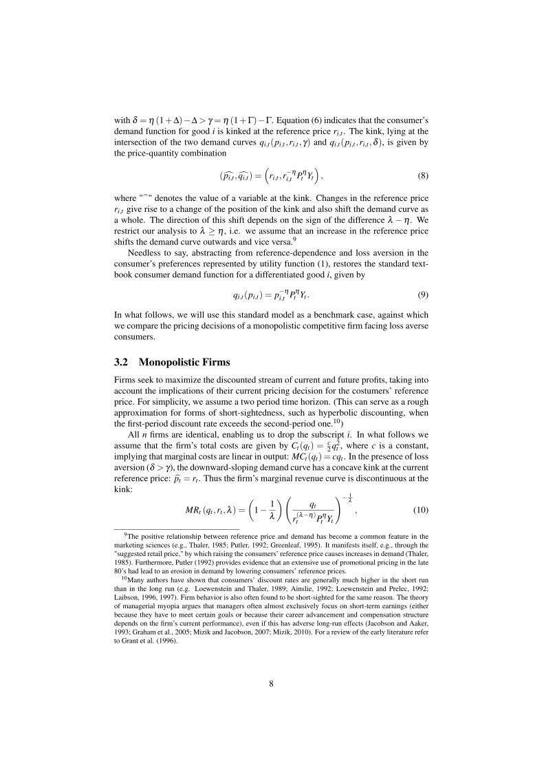
t , where c is a constant,implying that marginal costs are linear in output: MCt(qt) = cqt . In the presence of lossaversion (δ > γ), the downward-sloping demand curve has a concave kink at the currentreference price: pt = rt . Thus the firm’s marginal revenue curve is discontinuous at thekink:

MRt (qt ,rt ,λ ) =

(1− 1

λ

)(qt

r(λ−η)t Pη

t Yt

)− 1λ

, (10)

9The positive relationship between reference price and demand has become a common feature in themarketing sciences (e.g., Thaler, 1985; Putler, 1992; Greenleaf, 1995). It manifests itself, e.g., through the"suggested retail price," by which raising the consumers’ reference price causes increases in demand (Thaler,1985). Furthermore, Putler (1992) provides evidence that an extensive use of promotional pricing in the late80’s had lead to an erosion in demand by lowering consumers’ reference prices.

10Many authors have shown that consumers’ discount rates are generally much higher in the short runthan in the long run (e.g. Loewenstein and Thaler, 1989; Ainslie, 1992; Loewenstein and Prelec, 1992;Laibson, 1996, 1997). Firm behavior is also often found to be short-sighted for the same reason. The theoryof managerial myopia argues that managers often almost exclusively focus on short-term earnings (eitherbecause they have to meet certain goals or because their career advancement and compensation structuredepends on the firm’s current performance), even if this has adverse long-run effects (Jacobson and Aaker,1993; Graham et al., 2005; Mizik and Jacobson, 2007; Mizik, 2010). For a review of the early literature referto Grant et al. (1996).

8

pric

e

quantityqss∗

rss

= pss∗

marginal revenue curve (gaindomain)

demand curve (gaindomain)

marginal cost curve

marginal revenue curve (lossdomain)

demand curve (loss domain)

MRss

(qss∗ , r

ss, γ )

MRss

(qss∗ , r

ss, δ )

Figure 1: Initial steady state

with λ = γ for the gain domain and λ = δ for the loss domain, respectively. Theinterval [MRt (qt ,rt ,γ) , MRt (qt ,rt ,δ )], where MRt (qt ,rt ,γ) < MRt (qt ,rt ,δ ), we call“marginal revenue discontinuity” MRDt(qt ,rt ,γ,δ ).

We assume that in the initial steady state, the exogenously given reference priceis rss. Furthermore, in the steady state the firm’s marginal cost curve intersects themarginal revenue discontinuity, as depicted in Figure 1. To fix ideas, we assumethat initially the marginal cost curve crosses the midpoint of the discontinuity in themarginal revenue curve.11 This assumption permits us to derive the symmetry charac-teristics of the responses to positive and negative demand shocks. This implies that thefirm’s optimal price in the initial steady state p∗ss is equal to rss.12

4 Demand ShocksThe demand for each product i is subject to exogenous shocks, which may be temporaryor permanent. These demand shocks, represented by εt , are unexpected and enter thedemand function multiplicatively:

qt(pt ,rt ,λ ,εt) = r(λ−η)t p−λ

t Pη

t Ytεt . (11)

The corresponding marginal revenue functions of the firm are

MRt (qt ,rt ,λ ,εt) =

(1− 1

λ

)(qt

r(λ−η)t Pη

t Ytεt

)− 1λ

. (12)

We consider the effects of a demand shock that hits the economy in period t = 0.The demand shock shifts the marginal revenue curve, along with the marginal revenue

11To satisfy this condition, the slope parameter c of the marginal cost curve has to take the value c =1

2qss[MRt (qss,rss,γ)+MRt (qss,rss,δ )]

12The proof is straightforward: Let ν be an arbitrarily small number. Then for prices equal to rss +ν thefirm faces a situation in which marginal revenue is higher than marginal costs and decreasing the price wouldraise the firm’s profit, while for prices equal to rss−ν the firm faces a situation in which marginal revenue islower than marginal costs and increasing the price would raise the firm’s profit. Thus p∗ss = rss has to be theprofit maximizing price in the initial steady state.

9

discontinuity MRDt (qt ,rt ,γ,δ ,εt). We define a "small" shock as one that leaves themarginal cost curve passing through the marginal revenue discontinuity, and a "large"shock as one that shifts the marginal revenue curve sufficiently so that the marginalcost curve no longer passes through the marginal revenue discontinuity.

The maximum size of a small shock for the demand function (11) is

εt (λ ) =

(1− 1

λ

)r1+η

t

cPη

t Yt, (13)

i.e. εt (λ ) is the shock size for which the marginal cost curve lies exactly on the bound-aries of the shifted marginal revenue discontinuity MRDt (qt ,rt ,γ,δ ,εt (λ )).13 In theanalysis that follows, we will distinguish both between small and large demand shocksand between temporary and permanent demand shocks.

4.1 Temporary Demand ShocksFor a temporary (one-period) demand shock, the consumers’ reference price is not af-fected (since information reaches them with a one-period lag and they have rationalexpectations). Thus the firm’s price response to the shock is the same as that of a my-opic firm (which maximizes its current period profit).

Proposition 1: In response to a small temporary shock, prices remain rigid.

As noted, for a sufficiently small demand shock εs0 ≤ ε0 (λ ) the marginal cost curve

still intersects the marginal revenue discontinuity, i.e. MC0 (q0)∈MRD0(q0,rss,γ,δ ,ε

s0).

Therefore, the prevailing steady state price remains the firm’s profit-maximizing price,14

i.e. p∗0 = p∗ss, and we have complete price rigidity. By contrast, the profit-maximizingquantity changes to q∗0 = r−η

ss Pη

0 Y0εs0, thus the change of quantity is given by

∆q∗0 =q∗0q∗ss

=εs

0εss

= εs0 6= 1. (14)

This holds true irrespective of the sign of the small temporary demand shock.

Proposition 2: In response to a large temporary shock, prices are more sluggish up-wards than downwards.

For a large shock, i.e. ε l0 > ε0 (λ ), the marginal cost curve intersects the marginal

revenue curve outside the discontinuity of the latter. Consequently both, a price and aquantity reaction are induced. The new profit-maximizing price of the firm is

p∗0 =

(r(λ−η)

ss Pη

0 Y0ε l0

q∗0

) 1λ

, (15)

while its corresponding profit-maximizing quantity is

q∗0 =(

1c

(1− 1

λ

)) λ

λ+1 (r(λ−η)

ss Pη

0 Y0εl0

) 1λ+1

, (16)

13For ε (δ ), the marginal cost curve intersects the marginal revenue gap on the upper bound, whereas forε (γ) it intersects it on the lower bound.

14Compare the proof from Section 3.2.

10

where λ = δ for positive and λ = γ for negative shocks, respectively.In comparison to the standard firm the price reaction of the firm facing loss-averse

consumers in response to a large temporary demand shock is always smaller, whereasthe quantity reaction is always larger. Additionally, prices and quantities are less re-sponsive to positive than to negative shocks. The intuition is obvious once we decom-pose the demand shock into the maximum small shock and the remainder:

εl0 = ε0 (λ )+ ε

rem0 . (17)

From our theoretical analysis above, the maximum small shock ε0 (λ ) has no priceeffects, but feeds one-to-one into demand. This holds true irrespective of the sign ofthe shock. By contrast, the remaining shock εrem

0 has asymmetric effects. Let q0 be thequantity corresponding to ε0 (λ ). Then the change in quantity in response to εrem

0 isgiven by

∆qrem0 =

q∗0q0

=

(εrem

0ε0 (λ )

) 1λ+1

. (18)

As can be seen from equation 18, the change of quantity in response to εrem0 de-

pends negatively on λ , the price elasticity of demand. Since by definition δ > γ , thequantity reaction of the firm facing loss-averse consumers is smaller in response tolarge positive temporary demand shocks than to large negative ones. This however im-plies that prices are also less responsive to positive than to negative large temporarydemand shocks, because the former move the firm along the relatively flat portion ofthe demand curve, whereas the latter move it along the relatively steep portion of thedemand curve. This asymmetric sluggishness in the reaction to positive and negativelarge temporary demand shocks is a distinct feature of consumer loss aversion andstands in obvious contrast to the standard textbook case of monopoly pricing.

4.2 Permanent Demand ShocksNow consider a permanent, demand shock that occurs in period t = 0. Whereas the firmis assumed to change its price immediately in response to this shock, consumers updatetheir reference price in the following period t = 1, i.e. r1 = E0[p1]. Consequently, forprice increases (decreases) the demand curve shifts outwards (inwards) and the kinkmoves to

(p1, q1) =(r1,(P1/r1)

η Y1ε1). (19)

An outward shift of the demand curve (initiated by an upward adjustment in the refer-ence price) increases the firm’s long-run profits, whereas an inward shift (initiated by adownward adjustment of the reference price) lowers them. We term this phenomenonthe “reference-price updating effect.” The firm can anticipate this. Thus, it may havean incentive to set its price above the level that maximizes its profits in the shockperiod p′0 > p∗0, therewith exploiting (dampening) the outward (inward) shift of thedemand curve resulting from the upward (downward) adjustment of the consumers’reference price for positive (negative) permanent shocks.15 Whether this occurs de-pends on whether the firm’s gain from a price rise relative to p∗0 in terms of future

15Needless to say, setting a price lower than optimal in the shock period with the aim to decrease thereference price permanently is not a preferable option for the firm.

11

Parameter Symbol ValueDiscount rate β 0.99Elasticity of substitution η 5

implying substitutability ρ 0.8Price elasticity (gain domain) γ 6Price elasticity (loss domain) δ 12Loss aversion κ 2Exogenous nominal income Y 1Exogenous price index Pt 1

Table 1: Base calibration

profits (Π1(r1 = p′0)> Π1(r1 = p∗0), due to the relative rise in the reference price) ex-ceeds the firm’s loss in terms of present profits (Π0(p′0) < Π0(p∗0), since the price p′0is not appropriate for maximizing current profit).

To analyze which effect dominates, we calibrate the model and solve it numerically.

4.3 CalibrationWe calibrate the model for a quarterly frequency in accordance with standard values inthe literature. We assume an annual interest rate of 4 percent, which yields a discountfactor β = 0.99. We follow Schmitt-Grohé and Uribe (2007) and set the monopolisticmarkup to 25 percent, i.e. η = 5, which is also close to the value supported by Erceg etal. (2000) and which implies that goods are only little substitutable, i.e. ρ = 0.8. Sincewe impose λ ≥ η , we set γ = 6 in our base calibration. Loss aversion is measured bythe relative slopes of the demand curves in the gain and loss domain, i.e. κ = δ

γ. The

empirical literature on loss aversion in prices finds that losses induce demand reactionsapproximately twice as large as gains (Tversky and Kahnemann, 1991; Putler, 1992;Hardie et al., 1993; Griffin and Schulman, 2005; Adeyemi and Hunt, 2007). Therefore,we set κ = 2. The exogenous nominal income Y and price index Pt are normalized tounity.16 The base calibration is summarized in Table 1.

4.4 Numerical SimulationTables 2 and 3 present the numerical results of our base calibration in the two-periodmodel. In the tables we report the shock-arc-elasticities of price

(ηε,p =

%∆p%∆ε

)and

output(

ηε,q =%∆q%∆ε

)in the period of the shock t = 0 for positive and negative tempo-

rary and permanent shocks for the firm facing loss averse consumers.The results in Tables 2 and 3 confirm the theoretical analysis above for the tempo-

rary shock, summarized in Propositions 1 and 2. However, not all of these results carryover in the case of permanent demand shocks.

Proposition 3: For all permanent shocks, prices are less sluggish upwards than down-wards.

In line with the theoretical analysis above, our numerical results in table 2 and 3indicate that in the case of a permanent shock the firm exploits the "reference-price up-

16All results are completely robust to variations of these numerical values.

12

temporary shock permanent shockηε,p ηε,q ηε,p ηε,q

εs0 = 1.01 0 1 0.0100 0.8789

εs0 = 1.03 0 1 0.0667 0.1866

ε l0 = 1.05 0.0035 0.9560 0.0755 0.0717

ε l0 = 1.07 0.0232 0.7046 0.0790 0.0216

Table 2: Shock elasticities of price and output in t = 0 to positive permanent demandshocks, ε0 (γ) = 1.0476

temporary shock permanent shockηε,p ηε,q ηε,p ηε,q

εs0 = 0.99 0 1 0 1

εs0 = 0.97 0 1 0 1

ε l0 = 0.95 0.0072 0.9592 0.0012 0.9934

ε l0 = 0.93 0.0484 0.7264 0.0013 0.9927

Table 3: Shock elasticities of price and output in t = 0 to negative permanent demandshocks; ε0 (δ ) = 0.9524

dating effect" and generally sets a price that is higher than the price it would optimallyset in response to a temporary shock, i.e. p′0 > p∗0. For positive permanent demandshocks this implies that the pricing reaction of the firm is always stronger than forpositive temporary demand shocks for both, small17 and large shocks18. By contrast,for negative permanent demand shocks firms either do not adjust their prices at all forsufficiently small shocks or to a considerably lower extent than for negative temporaryshocks.

As a consequence, price sluggishness is considerably less pronounced for positivethan for negative permanent demand shocks. The asymmetry of the price reactionto positive and negative shocks therefore reverses, when moving from temporary topermanent shocks. While this result may seem surprising at first glance, it is straight-forward intuitively: As noted, for temporary shocks, consumers abstract from updatingtheir reference price. Therefore, the firm does not risk to suffer from a downward ad-justment of the consumers’ reference price, when encountering a temporary drop indemand with a price reduction. On the other hand, for positive temporary shocks, thefirm cannot generate permanent increases in demand due to upward-adjustments of thereference price. Since consumers react more sensitive to price increases relative to pricedecreases, the price and quantity reactions are smaller for positive temporary shockscompared to negative ones. By contrast, for permanent demand shocks, the firm ex-ploits the positive "reference-price updating effect" which follows from price increasesin response to positive shocks, whereas it tries to avoid the negative "reference-priceupdating effect" which follows from price decrease in response to negative shocks.19

17Of course, one can find a range of shocks, which are small enough to induce full price rigidity forpermanent positive shocks. Due to the reference-price updating effect, this threshold is, however, very small.Given the base calibration, the threshold value for a sufficiently small positive shock is ε0 (δ ) = 1.0087.

18Our numerical analysis indicates, however, that the positive reference-price updating effect is neverstrong enough to invalidate the general result that the pricing reaction of the firm facing loss averse consumersis more sluggish compared to the standard firm.

19Since the firm avoids price reductions, which lead to downward-adjustments in the reference price, but

13

5 ConclusionIn contrast to the standard time-dependent and state-dependent models of price slug-gishness, our theory of price adjustment is able to account for asymmetric price andquantity responses to positive and negative temporary and permanent shocks of equalmagnitude. In contrast to the New Keynesian literature, our explanation of price adjust-ment is thoroughly microfounded, without recourse to ad hoc assumptions concerningthe frequency of price changes or physical costs of price adjustments.

There are many avenues of future research. Consideration of heterogeneous firmsand multi-product firms will enable this model to generate asynchronous price changes,as well as the simultaneous occurrence of large and small price changes, and heteroge-neous frequency of price changes across products. Extending the model to a stochasticenvironment will generate testable implications concerning the variability of individ-ual prices. Furthermore, our model needs to be incorporated into a general equilibriumsetting to validate the predictions of our theory.

6 ReferencesAbeler, J., A. Falk, L. Goette, and D. Huffman (2011). Reference points and effortprovision. American Economic Review 101(2), 470-492.

Adeyemi, O.I. and L.C. Hunt (2007). Modelling OECD industrial energy demand:Asymmetric price responses and energy-saving technical change. Energy Economics29(4), 693-709.

Ainslie, G.W. (1992). Picoeconomics. Cambridge: Cambridge University Press.

Alvarez, L.J. and I. Hernando (2005). The price setting behavior of Spanish firms: Ev-idence from survey data. Working Paper Series 0538, European Central Bank.

Amirault, D., C. Kwan, and G. Wilkinson (2005). Survey of price-setting behaviour ofCanadian companies. Bank of Canada Review - Winter 2004-2005, 29-40.

Apel, M., R. Friberg, and K. Hallsten (2005). Microfoundations of macroeconomicprice adjustment: Survey evidence from Swedish firms. Journal of Money, Credit andBanking 37(2), 313-338.

Aucremanne, L. and M. Druant (2005). Price-setting behaviour in Belgium: What canbe learned from an ad hoc survey? Working Paper Series 0448, European Central Bank.

Ball, L. and N.G. Mankiw (1994). Asymmetric price adjustment and economic fluctu-ations. Economic Journal 104(423), 247-261.

Bidwell, M.O., B.R. Wang, and J.D. Zona (1995). An analysis of asymmetric demandresponse to price changes: The case of local telephone calls. Journal of RegulatoryEconomics 8(3), 285-298.

conducts price reductions, which do not influence the reference price, loss aversion offers a simple rationalefor the firm’s practice of “sales”(see e.g. Eichenbaum et al., 2011).

14

Blinder, A., E.R.D. Canetti, D.E. Lebow, and J.B. Rudd (1998). Asking about prices:A new approach to understanding price stickiness. New York: Russel Sage Foundation.

Caballero, R.J. and E.M.R.A. Engel (1993). Heterogeneity and output fluctuations in adynamic menu-cost economy. Review of Economic Studies 60(1), 95-119.

Caballero, R.J. and E.M.R.A. Engel (2007). Price stickiness in Ss models: New inter-pretations of old results. Journal of Monetary Economics 54(Supplement), 100-121.

Calvo, G.A. (1983). Staggered prices in a utility-maximizing framework. Journal ofMonetary Economics 12(3), 383-398.

Caplin, A.S. and D.F. Spulber (1987). Menu costs and the neutrality of money. TheQuarterly Journal of Economics 102(4), 703-725.

Card, D. and G.B. Dahl (2011). Family violence and football: The effect of unexpectedemotional cues on violent behavior. The Quarterly Journal of Economics 126(1), 103-143.

Cover, J.P. (1992). Asymmetric effects of positive and negative money-supply shocks.The Quarterly Journal of Economics 107(4), 1261-1282.

Crawford, V.P. and J. Meng (2011). New York City cab drivers’ labor supply revisited:Reference-dependent preferences with rational-expectations targets for hours and in-come. American Economic Review 101(5), 1912-1932.

DeLong, J.B. and L.H. Summers (1988). How does macroeconomic policy affect out-put? Brookings Papers on Economic Activity 19(2), 433-494.

Dixit, A.K. and J.E. Stiglitz (1977). Monopolistic competition and optimum productdiversity. American Economic Review 67(3), 297-308.

Dossche, M., F. Heylen, and D. Van den Poel (2010). The kinked demand curve andprice rigidity: Evidence from scanner data. Scandinavian Journal of Economics 112(4),723-752.

Dotsey, M., R.G. King, and A.L. Wolman (2009). Inflation and real activity with firmlevel productivity shocks. 2009 Meeting Papers 367, Society for Economic Dynamics.

Eichenbaum, M., N. Jaimovich, and S. Rebelo (2011). Reference prices, costs, andnominal rigidities. American Economic Review 101(1), 234-262.

Elmaghraby, W. and P. Keskinocak (2003). Dynamic pricing in the presence of in-ventory considerations: Research overview, current practices, and future directions.Management Science 49(10), 1287-1309.

Erceg, C.J., D.W. Henderson, and A.T. Levin (2000). Optimal monetary policy withstaggered wage and price contracts. Journal of Monetary Economics 46(2), 281-313.

15

Fabiani, S., M. Druant, I. Hernando, C. Kwapil, B. Landau, C. Loupias, F. Martins, T.Mathä, R. Sabbatini, H. Stahl, and A. Stockman (2006). What firm’s surveys tell usabout price-setting behavior in the Euro area. International Journal of Central Banking2(3), 1-45.

Fabiani, S., A. Gattulli, and R. Sabbatini (2004). The pricing behaviour of Italian firms:New survey evidence on price stickiness. Working Paper Series 0333, European Cen-tral Bank.

Genesove, D. and C. Mayer (2001). Loss aversion and seller behavior: Evidence fromthe housing market. The Quarterly Journal of Economics 116(4), 1233-1260.

Gertler, M. and J. Leahy (2008). A Phillips curve with an Ss foundation. Journal ofPolitical Economy 116(3), 533-572.

Golosov, M. and R.E. Lucas Jr. (2007). Menu costs and Phillips curves. Journal ofPolitical Economy 115(2), 171-199.

Graham, J.R., C.R. Harvey, and S. Rajgopal (2005). The economic implications ofcorporate financial reporting. Journal of Accounting and Economics 40(1-3), 3-73.

Grant, S., S. King, and B. Polak (1996). Information externalities, share-price basedincentives and managerial behaviour. Journal of Economic Surveys 10(1), 1-21.

Greenleaf, E.A. (1995). The impact of reference-price effects on the profitability ofprice promotions. Marketing Science 14(1), 82-104.

Greenslade, J.V. and M. Parker (2012). New insights into price-setting behaviour inthe UK: Introduction and survey results. Economic Journal 122(558), F1-F15.

Griffin, J.M. and C.T. Schulman (2005). Price asymmetry in energy demand models:A proxy for energy-saving technical change? The Energy Journal 0(2), 1-22.

Hall, R. and C. Hitch (1939). Price theory and business behaviour. Oxford EconomicPapers 2(1), 12-45.

Hall, S., M. Walsh, and A. Yates (2000). Are UK companies’ prices sticky? OxfordEconomic Papers 52(3), 425-446.

Hardie, B.G.S., E.J. Johnson, and P.S. Fader (1993). Modeling loss aversion and refer-ence dependence effects on brand choice. Marketing Science 12(4), 378-394.

Heidhues, P. and B. Koszegi (2005). The impact of consumer loss aversion on pricing.CEPR Discussion Papers No. 4849, Centre for Economic Policy Research.

Heidhues, P. and B. Koszegi (2008). Competition and price variation when consumersare loss averse. American Economic Review 98(4), 1245-1268.

Heidhues, P. and B. Koszegi (2014). Regular prices and sales. Theoretical Economics9(1), 217–251.

16

Hoeberichts, M. and A. Stokman (2010). Price setting behaviour in the Netherlands:Results of a survey. Managerial and Decision Economics 31(2-3), 135-149.

Jacobson, R. and D. Aaker (1993). Myopic management behavior with efficient, butimperfect, financial markets : A comparison of information asymmetries in the U.S.and Japan," Journal of Accounting and Economics 16(4), 383-405.

Kahneman, D. und A. Tversky (1979). Prospect theory: An analysis of decision underrisk. Econometrica 47(2), 263-291.

Kalwani, M.U., C.K. Yim, H.J. Rinne, and Y. Sugita (1990). A price expectationsmodel of customer brand choice. Journal of Marketing Research 27(3), 251-262.

Kalyanaram, G. and L.D.C. Little (1994). An empirical analysis of latitude of price ac-ceptance in consumer package goods. Journal of Consumer Research 21(3), 408-418.

Kandil, M. (1995). Asymmetric Nominal Flexibility and Economic Fluctuations. South-ern Economic Journal 61(3), 674-695.

Kandil, M. (1996). Sticky wage or sticky price? Analysis of the cyclical behavior ofthe real wage. Southern Economic Journal 63(2), 440-459.

Kandil, M. (1998). Supply-side asymmetry and the non-neutrality of demand fluctua-tions. Journal of Macroeconomics 20(4), 785-809.

Kandil, M. (1999). The asymmetric stabilizing effects of price flexibility: Historicalevidence and implications. Applied Economics 31(7), 825-839.

Kandil, M. (2001). Asymmetry in the effects of US government spending shocks:Evidence and implications. The Quarterly Review of Economics and Finance 41(2),137-165.

Kandil, M. (2002a). Asymmetry in the effects of monetary and government spendingshocks: Contrasting evidence and implications. Economic Inquiry 40(2), 288-313.

Kandil, M. (2002b). Asymmetry in economic fluctuations in the US economy: Thepre-war and the 1946–1991 periods compared. International Economic Journal 16(1),21-42.

Kandil, M. (2006). Asymmetric effects of aggregate demand shocks across U.S. indus-tries: Evidence and implications. Eastern Economic Journal 32(2), 259-283.

Kandil, M. (2010). The asymmetric effects of demand shocks: international evidenceon determinants and implications. Applied Economics 42(17), 2127-2145.

Karras, G. (1996). Why are the effects of money-supply shocks asymmetric? Convexaggregate supply or “pushing on a string”? Journal of Macroeconomics 18(4), 605-619.

17

Karras, G. and H.H. Stokes (1999). On the asymmetric effects of money-supply shocks:International evidence from a panel of OECD countries. Applied Economics 31(2),227-235.

Kehoe, P.J. and V. Midrigan (2008). Temporary price changes and the real effects ofmonetary policy. NBER Working Papers 14392, National Bureau of Economic Re-search, Inc.

Knetsch, J.L. and W.-K. Wong (2009). The endowment effect and the reference state:Evidence and manipulations. Journal of Economic Behavior & Organization 71(2),407-413.

Koszegi, B. and M. Rabin (2006). A model of reference-dependent preferences. TheQuarterly Journal of Economics 121(4), 1133-1165.

Koszegi, B. and M. Rabin (2007). Reference-dependent risk attitudes. American Eco-nomic Review 97(4), 1047-1073.

Koszegi, B. and M. Rabin (2009). Reference-dependent consumption plans. AmericanEconomic Review 99(3), 909-936.

Krishnamurthi, L., T. Mazumdar, and S.P. Raj (1992). Asymmetric response to pricein consumer brand choice and purchase quantity decisions. Journal of Consumer Re-search 19(3), 387-400.

Kwapil, C., J. Scharler, and J. Baumgartner (2010). How are prices adjusted in re-sponse to shocks? Survey evidence from Austrian firms. Managerial and DecisionEconomics 31(2-3), 151-160.

Laibson, D. (1996). Hyperbolic discount functions, undersaving, and savings policy.NBER Working Papers 5635, National Bureau of Economic Research, Inc.

Laibson, D. (1997). Golden eggs and hyperbolic discounting. The Quarterly Journalof Economics 112(2), 443-77.

Langbraaten, N., E.W. Nordbø, and F. Wulfsberg (2008). Price-setting behaviour ofNorwegian firms - Results of a survey. Norges Bank Economic Bulletin 79(2), 13-34.

Loewenstein, G. and D. Prelec (1992). Anomalies in intertemporal choice: Evidenceand an interpretation. The Quarterly Journal of Economics 107(2), 573-97.

Loewenstein, G. and R.H. Thaler (1989). Anomalies: Intertemporal choice. The Jour-nal of Economic Perspectives 3(4), 181-193.

Loupias, C. and R. Ricart (2004). Price setting in France: New evidence from surveydata. Working Paper Series 0423, European Central Bank.

Lünnemann, P. and T.Y. Mathä (2006). New survey evidence on the pricing behaviourof Luxembourg firms. Working Paper Series 0617, European Central Bank.

18

Martins, F. (2010). Price stickiness in Portugal evidence from survey data. Managerialand Decision Economics 31(2-3), 123-134.

Marzilli Ericson, K.M. and A. Fuster (2011). Expectations as endowments: Evidenceon reference-dependent preferences from exchange and valuation experiments. TheQuarterly Journal of Economics 126(4), 1879-1907.

Mas, A. (2006). Pay, reference pay and police performance. The Quarterly Journal ofEconomics 121(3), 783-821.

Maskin, E. and J. Tirole (1988). A theory of dynamic oligopoly, II: Price competition,kinked demand curves, and Edgeworth cycles. Econometrica 56(3), 571-99.

Mayhew, G.E and R.S. Winer (1992). An empirical analysis of internal and externalreference prices using scanner data. Journal of Consumer Research 19(1), 62-70.

McDonald, I.M. and H. Sibly (2001). How monetary policy can have permanent realeffects with only temporary nominal rigidity. Scottish Journal of Political Economy48(5), 532-46.

McDonald, I.M. and H. Sibly (2005). The diamond of macroeconomic equilibria andnon-inflationary expansion. Metroeconomica 56(3), 393-409.

Mehrara, M. and A.R. Karsalari (2011). Asymmetric effects of monetary shocks oneconomic activities: The case of Iran. Journal of Money, Investment and Banking 20,62-74.

Midrigan, V. (2011). Menu costs, multiproduct firms, and aggregate fluctuations.Econometrica 79(4), 1139-1180.

Mizik, N. (2010). The theory and practice of myopic management. Journal of Market-ing Research 47(4), 594-611.

Mizik, N. and R. Jacobson (2007). Myopic marketing management: Evidence of thephenomenon and its long-term performance consequences in the SEO context. Mar-keting Science 26(3), 361-379.

Morgan, A. (2008). Loss aversion and a kinked demand curve: Evidence from con-tingent behaviour analysis of seafood consumers. Applied Economics Letters 15(8),625-628.

Morgan, D.P. (1993). Asymmetric effects of monetary policy. Federal Reserve Bankof Kansas City Economic Review QII, 21-33.

Nasiry, N. and I. Popescu (2011). Dynamic pricing with loss-averse consumers andpeak-end anchoring. Operations Research 59(6), 1361-1368.

Nicolau, J.L. (2008). Testing reference dependence, loss aversion and diminishing sen-sitivity in Spanish tourism. Investigationes Económicas 32(2), 231-255.

19

Nicolitsas, D. (2013). Price setting practices in Greece: Evidence from a small-scalefirm-level survey. Working Papers 156, Bank of Greece.

Ólafsson, T.T., Á. Pétursdóttir, and K.Á. Vignisdóttir (2011). Price setting in turbulenttimes: Survey evidence from Icelandic firms. Working Paper No. 54, Central Bank ofIceland.

Okun, A.M. (1981). Prices and quantities: A macroeconomic analysis. Brookings In-stitution, Washington, DC.

Pope, D.G. and M.E. Schweitzer (2011). Is Tiger Woods loss averse? Persistent biasin the face of experience, competition, and high stakes. American Economic Review101(1), 129-157.

Popescu, I. and Y. Wu (2007). Dynamic pricing strategies with reference effects. Op-erations Research 55(3), 413-429.

Post, T., M.J. van den Assem, G. Baltussen, and R.H. Thaler (2008). Deal or no deal?Decision making under risk in a large-payoff game show. American Economic Review98(1), 38-71.

Putler, D.S. (1992). Incorporating reference price effects into a theory of consumerchoice. Marketing Science 11(3), 287-309.

Raman, K. and F.M. Bass (2002). A general test of reference price theory in the pres-ence of threshold effects. Tijdschrift voor Economie en Managerrient XLVII(2), 205-226.

Ravn, M.O. and M. Sola (2004). Asymmetric effects of monetary policy in the UnitedStates. Federal Reserve Bank of St. Louis Review 86(5), 41-60.

Rosenkranz, S. (2003). The manufacturer’s suggested retail price. CEPR DiscussionPapers 3954, C.E.P.R. Discussion Papers.

Rosenkranz, S. and P.W. Schmitz (2007). Reserve prices in auctions as referencepoints. Economic Journal 117(520), 637-653.

Rotemberg, J.J. (1982). Monopolistic price adjustment and aggregate output. Reviewof Economic Studies 49(4), 517-531.

Rotemberg, J.J. (2005). Customer anger at price increases, changes in the frequency ofprice adjustment and monetary policy. Journal of Monetary Economics 52(4), 829-852.

Rotemberg, J.J. (2010). Altruistic dynamic pricing with customer regret. ScandinavianJournal of Economics 112(4), 646-672.

Ryan, D.L. and A. Plourde (2007). A systems approach to modelling asymmetric de-mand responses to energy price changes. In: W. A. Barnett and A. Serletis (eds.), In-ternational Symposia in Economic Theory and Econometrics, Volume 18, pp. 183-224.

20

Sahinöz, S. and B. Saraçoglu (2008). Price-setting behavior In Turkish industries: Ev-idence from survey data. The Developing Economies 46(4), 363-385.

Schmitt-Grohé, S. and M. Uribe (2007). Optimal simple and implementable monetaryand fiscal rules. Journal of Monetary Economics 54(6), 1702-1725.

Sheshinski, E. and Y. Weiss (1977). Inflation and costs of price adjustment. Review ofEconomic Studies 44(2), 287-303.

Sibly, H. (1996). Consumer disenchantment, loss aversion and price rigidity. Papers1996-12, Tasmania - Department of Economics.

Sibly, H. (2002). Loss averse customers and price inflexibility. Journal of EconomicPsychology 23(4), 521-538.

Sibly, H. (2007). Loss aversion, price and quality. The Journal of Socio-Economics36(5), 771-788.

Spiegler, R. (2012). Monopoly pricing when consumers are antagonized by unexpectedprice increases: A “cover version” of the Heidhues-Koszegi-Rabin model. EconomicTheory 51(3), 695-711.

Stahl, H. (2005). Price setting in German manufacturing: New evidence from new sur-vey data. Working Paper Series 0561, European Central Bank.

Sweezy, P. (1939). Demand under conditions of oligopoly. The Journal of PoliticalEconomy 47(4), 568-573.

Tan, S.-H., M.-S. Habibullah, and A. Mohamed (2010). Asymmetric effects of mon-etary policy in ASEAN-4 economies. International Research Journal of Finance andEconomics 44, 30-42.

Taylor, J.B. (1979). Staggered wage setting in a macro model. American EconomicReview 69(2), 108-113.

Thaler, R. (1985). Mental accounting and consumer choice. Marketing Science 4(3),199-214.

Thaler, R. (1991). Quasi rational economics. Russell Sage Foundation, New York.

Thoma, M.A. (1994). Subsample instability and asymmetries in money-income causal-ity. Journal of Econometrics 64(1-2), 279-306.

Tversky, A. and D. Kahneman, D. (1991). Loss aversion in riskless choice: A reference-dependent model. The Quarterly Journal of Economics 106(4), 1039-1061.

Weise, C.L. (1999). The asymmetric effects of monetary policy: A nonlinear vectorautoregression approach. Journal of Money, Credit and Banking 31(1), 85-108.

21

Zbaracki, M.J., M. Ritson, D. Levy, S. Dutta, and M. Bergen (2004). Managerial andcustomer costs of price adjustment: Direct evidence from industrial markets. The Re-view of Economics and Statistics 86(2), 514-533.

Zhou, J. (2011). Reference dependence and market competition. Journal of Economics& Management Strategy 20(4), 1073-1097.

Appendix

1. Demand Curve of Loss Averse ConsumersThe loss averse consumer maximizes her utility function (1) subject to her budget con-straint (3). The corresponding Lagrangian problem reads:

maxqi,t

L =

[n

∑i=1

((pi,t

ri,t

)−µ

qi,t

)ρ] 1ρ

−ϕ

[n

∑i=1

pi,tqi,t −PtYt

], (20)

where ϕ is the Lagrangian multiplier. The first-order condition of the Lagrangian func-tion (20) is

∂Lt

∂qi,t=

1ρ

[n

∑i=1

((pi,t

ri,t

)−µ

qi,t

)ρ] 1ρ−1(

pi,t

ri,t

)−µρ

qρ−1i,t ρ−ϕ pi,t = 0. (21)

We collect all terms including demand components on the left hand side

qρ−1i,t

[n

∑i=1

((pi,t

ri,t

)−µ

qi,t

)ρ] 1−ρ

ρ

= ϕ pi,t

(pi,t

ri,t

)µρ

, (22)

and simplify the exponentials

qi,t

[n

∑i=1

((pi,t

ri,t

)−µ

qi,t

)ρ]− 1ρ

=

(ϕ pi,t

(pi,t

ri,t

)µρ) 1ρ−1

. (23)

We define overall demand according to a Dixit and Stiglitz (1977) aggregate, whichreads

qt =

[n

∑i=1

((pi,t

ri,t

)−µ

qi,t

)ρ] 1ρ

. (24)

Applying (24) as well as the definition of the elasticity of substitution (i.e. η = 11−ρ

),we can simplify (23) to

qi,t = (ϕ pi,t)−η

(pi,t

ri,t

)−µ(η−1)

qt . (25)

To determine the Lagrangian multiplier ϕ , we plug (25) into (24)

qt =

n

∑i=1

((pi,t

ri,t

)−µ

(ϕ pi,t)−η

(pi,t

ri,t

)−µ(η−1)

qt

) η−1η

η

η−1

, (26)

22

which after some simple manipulations yields

ϕ =

n

∑i=1

(pi,t

/(pi,t

ri,t

)−µ)1−η

1η−1

≡ P−1t . (27)

We define the inverse of the Lagrangian multiplier ϕ as the overall price index Pt .Plugging (27) back into (25) yields

qi,t = Pη

t

(pi,t

ri,t

)−µ(η−1)

p−η

i,t qt . (28)

Applying the budget constraint (3) yields

qi,t = Pη

t

(pi,t

ri,t

)−µ(η−1)

p−η

i,t Yt . (29)

Finally, we simplify (29) using the definition λ = η(1 + µ)− µ , which yields thedemand curve for the differentiated good i

qi,t = rλ−η

i,t p−λ

i,t Pη

t Yt (30)

Including the shock term, equation (30) reads

qi,t = rλ−η

i,t p−λ

i,t Pη

t Ytεt . (31)

2. Price and Quantity at the KinkThe kink is given by the particular price at which the two demand curves intersect, i.e.qi,t(pi,t ,ri,t ,γ) = qi,t(pi,t ,ri,t ,δ ). Given (31) and the definition of λ from equation (7)it must hold that

rγ−η

i,t p−γ

i,t Pη

t Ytεt = rδ−η

i,t p−δ

i,t Pη

t Ytεt , (32)

which simplifies torγ−η

i,t p−γ

i,t = rδ−η

i,t p−δ

i,t . (33)

Sorting terms yieldspδ−γ

i,t = rδ−η−γ+η

i,t . (34)

From (34) it is obvious that pi,t = ri,t at the kink. Plugging (34) back into (31) givesthe quantity at the kink

qi,t = r−η

i,t Pη

t Ytεt . (35)

23

6.1 3. Demand Curve of Standard ConsumersThe standard consumer (i.e. the non-loss averse consumer) maximizes her utility func-tion

Ut (q1,t , ...,qn,t) =

[n

∑i=1

qρ

i,t

] 1ρ

, (36)

subject to her budget constraint (3). The corresponding Lagrangian problem reads:

maxqi,t

L =

[n

∑i=1

qρ

i,t

] 1ρ

−φ

[n

∑i=1

pi,tqi,t −PtYt

], (37)

where φ is the Lagrangian multiplier for the standard textbook problem. The first-ordercondition of the Lagrangian problem (37) is

∂Lt

∂qi,t=

1ρ

[n

∑i=1

qρ

i,t

] 1ρ−1

qρ−1i,t ρ−φ pi,t = 0. (38)

We collect all terms including demand components on the left hand side and simplifythe exponentials

qi,t

[n

∑i=1

qρ

i,t

]− 1ρ

= (φ pi,t)1

ρ−1 . (39)

We define overall demand for the standard consumer by a Dixit and Stiglitz (1977)aggregate of the form

qt =

[n

∑i=1

qρ

i,t

] 1ρ

. (40)

Applying (40) as well as the definition of the elasticity of substitution, we can simplify(39) to

qi,t = (φ pi,t)−η qt . (41)

To determine the Lagrangian multiplier φ , we plug (41) into (40)

qt =

[n

∑i=1

((φ pi,t)

−η qt) η−1

η

] η

η−1

, (42)

which after some simple manipulations yields

φ =

[n

∑i=1

p1−η

i,t

] 1η−1

≡ P−1t . (43)

We define the inverse of the Lagrangian multiplier φ as the overall price index Pt forthe standard textbook problem. Plugging (43) back into (41) yields

qi,t = Pη

t p−η

i,t qt . (44)

Applying the budget constraint (3) yields the demand curve for the differentiated goodi for the standard consumer

qi,t = p−η

i,t Pη

t Yt (45)

24

Including the shock term, equation (45) reads

qi,t = p−η

i,t Pη

t Ytεt . (46)

4. Marginal Revenue CurveSince all firms are assumed to be identical, we drop the subscript i for the firm deriva-tions. Revenue is given by

Rt = pt(qt ,rt ,λ ,εt)qt =

(qt

r(λ−η)t Pη

t Ytεt

)− 1λ

qt , (47)

or in short

Rt =(

r(λ−η)t Pη

t Ytεt

) 1λ q

1− 1λ

t . (48)

The first-order condition with respect to qt yields the marginal revenue curve

MRt =∂Rt

∂qt=

(1− 1

λ

)(qt

r(λ−η)t Pη

t Ytεt

)− 1λ

. (49)

5. Critical Shock SizeThe critical value for the small shock is given by the particular shock εt (λ ), for whichthe marginal cost curve exactly intersects the critical bounds of the shifted marginalrevenue discontinuity, i.e.

MCt (q∗t )!= MRt (q∗t ,rt ,λ ,εt (λ )) , (50)

where MCt(qt) =∂C(qt )

∂qt= cqt , with Ct(qt) =

c2 q2

t . Evaluating the marginal revenuecurve (49) and the marginal cost curve at the post-shock optimum yields

cq∗t =(

1− 1λ

)(q∗t

ε (λ )r(λ−η)t Pη

t Yt

)− 1λ

. (51)

From the analysis of small shocks we know that the new quantity of the maximumsmall shock is q∗t = εt (λ )r−η

t Pη

t Yt . Applying this, we obtain

cεt (λ )r−η

t Pη

t Yt =

(1− 1

λ

)(εt (λ )r−η

t Pη

t Yt

εt (λ )r(λ−η)t Pη

t Yt

)− 1λ

. (52)

Solving for εt (λ ) yields the critical shock size

εt (λ ) =

(1− 1

λ

)r1+η

t

cPη

t Yt. (53)

25

6. Optimal Price and Quantity in Reaction to a Large Shock for theMyopic FirmThe new optimal price lies at the intersection of the marginal cost curve with the shiftedmarginal revenue curve, which by definition is outside the marginal revenue disconti-nuity

MCt (q∗t ,εt) = MRt (q∗t ,rt ,λ ,εt) . (54)

Applying the respective functions yields

cq∗t =(

1− 1λ

)(q∗t

r(λ−η)t Pη

t Ytεt

)− 1λ

. (55)

Solving this equation for q, we obtain

q∗t =(

1c

(1− 1

λ

)) λ

λ+1 (r(λ−η)

t Pη

t Ytεt

) 1λ+1

. (56)

The optimal price can be calculated by plugging q∗t into the inverse demand curve,given by

p∗t =

(q∗t

r(λ−η)t Pη

t Ytεt

)− 1λ

. (57)

26

SFB 649 Discussion Paper Series 2014

For a complete list of Discussion Papers published by the SFB 649,

please visit http://sfb649.wiwi.hu-berlin.de.

001 "Principal Component Analysis in an Asymmetric Norm" by Ngoc Mai

Tran, Maria Osipenko and Wolfgang Karl Härdle, January 2014.

002 "A Simultaneous Confidence Corridor for Varying Coefficient Regression

with Sparse Functional Data" by Lijie Gu, Li Wang, Wolfgang Karl Härdle

and Lijian Yang, January 2014.

003 "An Extended Single Index Model with Missing Response at Random" by

Qihua Wang, Tao Zhang, Wolfgang Karl Härdle, January 2014.

004 "Structural Vector Autoregressive Analysis in a Data Rich Environment:

A Survey" by Helmut Lütkepohl, January 2014.

005 "Functional stable limit theorems for efficient spectral covolatility

estimators" by Randolf Altmeyer and Markus Bibinger, January 2014.

006 "A consistent two-factor model for pricing temperature derivatives" by

Andreas Groll, Brenda López-Cabrera and Thilo Meyer-Brandis, January

2014.

007 "Confidence Bands for Impulse Responses: Bonferroni versus Wald" by

Helmut Lütkepohl, Anna Staszewska-Bystrova and Peter Winker, January

2014.

008 "Simultaneous Confidence Corridors and Variable Selection for

Generalized Additive Models" by Shuzhuan Zheng, Rong Liu, Lijian Yang

and Wolfgang Karl Härdle, January 2014.

009 "Structural Vector Autoregressions: Checking Identifying Long-run

Restrictions via Heteroskedasticity" by Helmut Lütkepohl and Anton

Velinov, January 2014.

010 "Efficient Iterative Maximum Likelihood Estimation of High-

Parameterized Time Series Models" by Nikolaus Hautsch, Ostap Okhrin

and Alexander Ristig, January 2014.

011 "Fiscal Devaluation in a Monetary Union" by Philipp Engler, Giovanni

Ganelli, Juha Tervala and Simon Voigts, January 2014.

012 "Nonparametric Estimates for Conditional Quantiles of Time Series" by

Jürgen Franke, Peter Mwita and Weining Wang, January 2014.

013 "Product Market Deregulation and Employment Outcomes: Evidence

from the German Retail Sector" by Charlotte Senftleben-König, January

2014.

014 "Estimation procedures for exchangeable Marshall copulas with

hydrological application" by Fabrizio Durante and Ostap Okhrin, January

2014.

015 "Ladislaus von Bortkiewicz - statistician, economist, and a European

intellectual" by Wolfgang Karl Härdle and Annette B. Vogt, February

2014.

016 "An Application of Principal Component Analysis on Multivariate Time-

Stationary Spatio-Temporal Data" by Stephan Stahlschmidt, Wolfgang

Karl Härdle and Helmut Thome, February 2014.

017 "The composition of government spending and the multiplier at the Zero

Lower Bound" by Julien Albertini, Arthur Poirier and Jordan Roulleau-

Pasdeloup, February 2014.

018 "Interacting Product and Labor Market Regulation and the Impact of

Immigration on Native Wages" by Susanne Prantl and Alexandra Spitz-

Oener, February 2014.

SFB 649, Spandauer Straße 1, D-10178 Berlin


This research was supported by the Deutsche

Forschungsgemeinschaft through the SFB 649 "Economic Risk".










For a complete list of Discussion Papers published by the SFB 649, please visit http://sfb649.wiwi.hu-berlin.de.

019 "Unemployment benefits extensions at the zero lower bound on nominal

interest rate" by Julien Albertini and Arthur Poirier, February 2014.

020 "Modelling spatio-temporal variability of temperature" by Xiaofeng Cao,

Ostap Okhrin, Martin Odening and Matthias Ritter, February 2014.

021 "Do Maternal Health Problems Influence Child's Worrying Status?

Evidence from British Cohort Study" by Xianhua Dai, Wolfgang Karl

Härdle and Keming Yu, February 2014.

022 "Nonparametric Test for a Constant Beta over a Fixed Time Interval" by

Markus Reiß, Viktor Todorov and George Tauchen, February 2014.

023 "Inflation Expectations Spillovers between the United States and Euro

Area" by Aleksei Netšunajev and Lars Winkelmann, March 2014.

024 "Peer Effects and Students’ Self-Control" by Berno Buechel, Lydia

Mechtenberg and Julia Petersen, April 2014.

025 "Is there a demand for multi-year crop insurance?" by Maria Osipenko,

Zhiwei Shen and Martin Odening, April 2014.

026 "Credit Risk Calibration based on CDS Spreads" by Shih-Kang Chao,

Wolfgang Karl Härdle and Hien Pham-Thu, May 2014.

027 "Stale Forward Guidance" by Gunda-Alexandra Detmers and Dieter

Nautz, May 2014.

028 "Confidence Corridors for Multivariate Generalized Quantile Regression"

by Shih-Kang Chao, Katharina Proksch, Holger Dette and Wolfgang

Härdle, May 2014.

029 "Information Risk, Market Stress and Institutional Herding in Financial

Markets: New Evidence Through the Lens of a Simulated Model" by

Christopher Boortz, Stephanie Kremer, Simon Jurkatis and Dieter Nautz,

May 2014.

030 "Forecasting Generalized Quantiles of Electricity Demand: A Functional

Data Approach" by Brenda López Cabrera and Franziska Schulz, May

2014.

031 "Structural Vector Autoregressions with Smooth Transition in Variances –

The Interaction Between U.S. Monetary Policy and the Stock Market" by

Helmut Lütkepohl and Aleksei Netsunajev, June 2014.

032 "TEDAS - Tail Event Driven ASset Allocation" by Wolfgang Karl Härdle,

Sergey Nasekin, David Lee Kuo Chuen and Phoon Kok Fai, June 2014.

033 "Discount Factor Shocks and Labor Market Dynamics" by Julien Albertini

and Arthur Poirier, June 2014.

034 "Risky Linear Approximations" by Alexander Meyer-Gohde, July 2014

035 "Adaptive Order Flow Forecasting with Multiplicative Error Models" by

Wolfgang Karl Härdle, Andrija Mihoci and Christopher Hian-Ann Ting,

July 2014

036 "Portfolio Decisions and Brain Reactions via the CEAD method" by Piotr

Majer, Peter N.C. Mohr, Hauke R. Heekeren and Wolfgang K. Härdle, July

2014

037 "Common price and volatility jumps in noisy high-frequency data" by

Markus Bibinger and Lars Winkelmann, July 2014

038 "Spatial Wage Inequality and Technological Change" by Charlotte

Senftleben-König and Hanna Wielandt, August 2014

039 "The integration of credit default swap markets in the pre and post-

subprime crisis in common stochastic trends" by Cathy Yi-Hsuan Chen,

Wolfgang Karl Härdle, Hien Pham-Thu, August 2014







040 "Localising Forward Intensities for Multiperiod Corporate Default" by

Dedy Dwi Prastyo and Wolfgang Karl Härdle, August 2014.

041 "Certification and Market Transparency" by Konrad Stahl and Roland

Strausz, September 2014.

042 "Beyond dimension two: A test for higher-order tail risk" by Carsten

Bormann, Melanie Schienle and Julia Schaumburg, September 2014.

043 "Semiparametric Estimation with Generated Covariates" by Enno

Mammen, Christoph Rothe and Melanie Schienle, September 2014.

044 "On the Timing of Climate Agreements" by Robert C. Schmidt and

Roland Strausz, September 2014.

045 "Optimal Sales Contracts with Withdrawal Rights" by Daniel Krähmer and

Roland Strausz, September 2014.

046 "Ex post information rents in sequential screening" by Daniel Krähmer

and Roland Strausz, September 2014.

047 "Similarities and Differences between U.S. and German Regulation of the

Use of Derivatives and Leverage by Mutual Funds – What Can Regulators

Learn from Each Other?" by Dominika Paula Gałkiewicz, September

2014.

048 "That's how we roll: an experiment on rollover risk" by Ciril Bosch-Rosa,

September 2014.

049 "Comparing Solution Methods for DSGE Models with Labor Market

Search" by Hong Lan, September 2014.

050 "Volatility Modelling of CO2 Emission Allowance Spot Prices with Regime-

Switching GARCH Models" by Thijs Benschop, Brenda López Cabrera,

September 2014.

051 "Corporate Cash Hoarding in a Model with Liquidity Constraints" by Falk

Mazelis, September 2014.

052 "Designing an Index for Assessing Wind Energy Potential" by Matthias

Ritter, Zhiwei Shen, Brenda López Cabrera, Martin Odening, Lars

Deckert, September 2014.

053 "Improved Volatility Estimation Based On Limit Order Books" by Markus

Bibinger, Moritz Jirak, Markus Reiss, September 2014.

054 "Strategic Complementarities and Nominal Rigidities" by Philipp König,

Alexander Meyer-Gohde, October 2014.

055 "Estimating the Spot Covariation of Asset Prices – Statistical Theory and

Empirical Evidence” by Markus Bibinger, Markus Reiss, Nikolaus Hautsch,

Peter Malec, October 2014.

056 "Monetary Policy Effects on Financial Intermediation via the Regulated

and the Shadow Banking Systems" by Falk Mazelis, October 2014.

057 "A Tale of Two Tails: Preferences of neutral third-parties in three-player

ultimatum games" by Ciril Bosch-Rosa, October 2014.

058 "Boiling the frog optimally: an experiment on survivor curve shapes and

internet revenue" by Christina Aperjis, Ciril Bosch-Rosa, Daniel

Friedman, Bernardo A. Huberman, October 2014.

059 "Expectile Treatment Effects: An efficient alternative to compute the

distribution of treatment effects" by Stephan Stahlschmidt, Matthias

Eckardt, Wolfgang K. Härdle, October 2014.

060 "Are US Inflation Expectations Re-Anchored?" by Dieter Nautz, Till

Strohsal, October 2014.







061 "Why the split of payroll taxation between firms and workers matters for

macroeconomic stability" by Simon Voigts, October 2014.

062 "Do Tax Cuts Increase Consumption? An Experimental Test of Ricardian

Equivalence" by Thomas Meissner, Davud Rostam-Afschar, October

2014.

063 "The Influence of Oil Price Shocks on China’s Macro-economy : A

Perspective of International Trade" by Shiyi Chen, Dengke Chen,

Wolfgang K. Härdle, October 2014.

064 "Whom are you talking with? An experiment on credibility and

communication structure" by Gilles Grandjean, Marco Mantovani, Ana

Mauleon, Vincent Vannetelbosch, October 2014.

065 "A Theory of Price Adjustment under Loss Aversion" by Steffen Ahrens,

Inske Pirschel, Dennis J. Snower, November 2014.

I L R A Theory of Price E B Adjustment under Loss Aversion

Documents

Transcript of I L R A Theory of Price E B Adjustment under Loss Aversion