AD-A124 706 AN ANALYSIS OF THE SPACE TRANSPORTATION SYSTEM LAUNCH I/RATE CAPABILITY UTI..(U) AIR FORCE INST OF TECHWRIGHT-PATTERSON AFB OH SCHOOL OF ENGI..

UNCLASSIFIED J G ANDRUSYSZYN ET AL. DEC 82 F/G 9/2 NL

IIIIEEmEIIIsmmhhhhhhmuoEoommhhhhmhmEmhhmhhEohhhIEhEEEmhhhhEEEIEhmhEmhEmhohhI

EEEIIEIIIIIII

I i1.0 IL 328 LIS

MICROCoPY RESOLUTION TEST CHARTNATIONAL BUJR _AU OF SThNOARS9

3 .A -

RiQ 6 IS1,2.0

1. 3l2

At

AV4,

AriT/,so/o/82D- -

AN ANALYSIS O THE SPA( TRANSPOR ATION

SYSTEM I NCH RATE CAPABILITY UTILIZING

Q-GER? SIMULATION TECHNIQUES

John C, AmJrusyssyn Brian C, Millburn

Capt USAF Capt USAF D1TIC

i, m% FEB 2 2 1983

AAplmoved foz publio isles.o; diti~lbutica UEnlIUte4

14

APXT/Gso/os/82D-1

AN ANALYSIS Or THE SPACR TRANSPORTATION 31311K

LAUNCH RATE CAPABILITY

UTILIZING Q-GERT SIMIATIOK TZWNIWIS

TIISIS

Presented to the Faculty of the School of egineerin

of the Air For Institute of Technology

Air University

inPartial ruifilient, of the

Requirements for the Degree of

Masters of Science

by

John C Andrusyssyn, ,.S3o

Capt USAr

Graduate SpaOe Operations

and

Raw C. millburn* B.S.

Capt USA?

Graduate Spam Operations,

December 1962

(Approved fo public releme diatribution unlimited,

Preface

As students In the Air foros Institute of Technology's Graduate

program in space Operations, we ar. quite interested in the progess

of the Spa Transportation system. This system will be the primary

mans of launching DoD payloads Into earth orbit, In fact@ DOD

payload. will fly on up to half of all flights after 1988. Therefore,

any -short falls the system may have In launch rate capability will

have a big Impact on DoD. A review of the trade literature indicated

that the system has already reached the point of saturation and that

NASA has been unable to fund the hardware procurement and facility

t construction needed to Increase the system launch rate to & level

sufficient to meet user needs, Therefore, additionalop atel

funding will have to be applied to the system In the near future. As

this funding ts bound to be limited, It must be wisely spent on thoe

portion& of the system which will contribute greatest to incrasing

the launch rate, The purpose of our thesis was to develop a launch

rate enhancement plan which will present tfie proper sequence In which

flight hardware and facilities should be added., This plan.-also had to

provide accurate estimates of STS launch rate capability given various

configurations of hardware and facilitiles. Theref ore, the problem was

to develop a method which would acourately predict STS launch rate

capability wa Identify the bottlenecks in the system. Two sash

methods were devised. The analytic mthod was originally Intended for

use in validating the simulation results, but It was found to be

accurate enough to Ie useful ty itself, Of cours, If the mest

accurate results an desired, the simulation method Is the one to ue

(. The launch enhancement pAm developed from the two models Is preasid

MOMi

In Chapter Vlo As expected, the capaity of the system to loe than

that anticipated by the current flight schedule, The plan am theref ore

be used as a guide to determiam what facilties and hardware to add to

met the scheduled flights, In addition, It provides planners with &

tool to judge the financial, viabilty of mtIng various lauanch rates,

We would like to thank our Advisor, Major Joseph oleman at AIT$

for his guidance In preparing this work, Ve would also like to expess

cur sincere thanks to Mr, Herbert Fogarty Of Rockwell International,

and Mrs Porter DrIde.l and, Mr. Vince Caruso of George C. Marshall

Spaceflight Oenter for their kind help In providing the data needed to

prepare this report. Finally, we would lke to thank our wives and

kids for putting up with us during the preparation of this thoess

Cl

Contents

Pref ace * o o * ,o o o o ,o * o , , * * o * * * o o , o o 1 o

List of Abbreviations . * , * ,, * , ee, ,, , vi

List of Figures . .*,,, * ,,,, e ,.. *. *. g. vii

List of Tables . • • • * • .• . .9 e e • • evii

Abstract . , , e., ,*o , , . g. x

I, Introduction e e a , * e . e , e 9 e 9 e , 1

Problem and Scope . ,... ,g .. ..... . . 2General Approach • e • * • a * • . • • • • . • . • • • 3Sequenoe of Presentation, . . . . , , , . , , , .0 a 3Assumptions . , 9 a e . 9 * 9 a , . . . , , a * , 0 a , 4Literature Review . . . . . . . . . . . . . . . . . . 5

II. STS System Description . . . . . . . , , . . , , , . , , . 7Kennedy Space Center, , , , , , . , , , . , . , . * , 7Vandenberg AFB * e & . , *..... e a . .. ., 8

SRB and External Tank e g...• .. & a . • • • * • * a 9

TIo, Research Design . .. , • .. . . .. . . . 12

Research Design Considerations , e , , , , ., , , , , 12Response Variable , . .. , . 13Factors , * . . . • . . . . . , . . . . , , . . , . 13Additional ;oncerns • 0 o 14

Q-GERT Simulation Techniques. . . 15Q-GEBT Description . . . . . . . . . 15Q-GERT Facilities . . . . . . .. 17

Structural and Parametric Models . * 21VAFB Structural Model .e 0 9 9 0 9 e e 9 22VAB Parametric Model o . . . . .. e , .. .. 24KSC Structural Model . , , , . , . . . . . , o . 26KSC Parametric Model . . . . . . . . . . . 32

Experimental Design . ,..,a.......... 35

IV, Verification and Validation o .,. .. , • , . 42

Assumptions 4 3Model . * * * e a a o , , p , . , , 9 46 .,.Resuats . . . , , . . . , . , . , . . . . . . . 6

V, Analytic Approach e •e• e e 49

Analytic Network. 9.. . .o o 9 9. 50

AJI t O •• ••• ••• •• ••i 5

contents

(continued)

Page

Capacities . * 0 a a * . * * * * 0 * * 51VAB High Day Capacity *..... ..... .... 52ELP Capacity .t . * * 56

PS' Capacity.. . . . . . .& . 60Orbiter Capacity * * , * * a a . . e . o o e o 61ON' Capacity . . . . . . . . . . . . . . . . . . . . 6Launch Pad Capacity e % .o * e " * e * e " * * " " 66ST and SR .Ca ities . . . . . . . . . 0 0 0 0 0 , 66LaunchEnhancement Plan . .. . . . . . . . 66

I. Application and Analyysis . .si . . . . 72

VAFB ModelAnalysis **... ,.. . , . . 72SensitivityAnalysis .al•. .. .. . 72Model Results . e . • • • • • • • • • • • • • • • 75

KSC Model Analysis . . . . . • . . . . . . . . . . . . 76Sensitivity Analysis . . . . . . . . . . 76Sample Analysis and Results . . . . . ....... 84

VII. Conclusions , ,,.o. .eo, ,, . 92

Analytic vs iimulation................. 93Launch Enhancement Plan . . . . .. .... • 95

VIII, Recommendations . • e a * • . • • • • • • • . • • • , • • 97

Bibliography . . . . . . . . . . 0 0 * 0 a , 0 9B

Appendix As KSC Q-GERT Simulation Model and Results . . . t . . . O0

Appendix Be VAFB Q-ERT Simulation Model. ............ 129

VITA .140

v!

List of Abbreviations

LT Nxternal Tank

KSC Kennedy Space Center

OM Orbiter Maintenance and Checkout Facility (Vandenberg AFB)

OPP Orbiter Processing Facility (Kennedy Space center)

PS, Processing and Storage Facility (SRBs)

S M Solid Rocket Motor

SRB Solid Rocket Booster

STAR Shuttle Turnaround Analysis Report (Kennedy Space Center)

VAPB Vandenberg AFB

VSTAR Vandenberg AFB Shuttle Turnaround Analysis Report

ivi

List of Figures

SKSC STS Flow . .. . . . . . . . . . . . 10

2 VAFBS513 o ..... . e.. .oo. e..... . 11

3 STS Analytio Network . . . . . . . . . . . . . . . .. . . 50

4& Simulation Model SWp leOutput A . . . . .. . • 0 . . 85

5 Simulation Model Sample Output B . . . . . . . . . ... . . 86

6 xsecanTcrphiaal odel . 0...0.0.*...0.&.& .1017 VAB Q-W Gr~Zaphial odel . . . . . . . . . . . . . . . . . 1017 VAP3QB -Gr raphcaModel........... ...... 130

vilL

eList of Tables

I Activity Times * . * * * * * * * . * . * , . * * * . , * * 51

II VAS H HIhBa y Capacity . . . . . . . . . . . . . . . . . . 55

III )P Capacity. *. .. . g0... 0 0 57

IV NLP Capacity(Adjusted) . . . . . . . . . . . . . . . . . 58

V 3T C/O Cell Capacity .. .. .. .. . .. . . . . .* * 59

VI ITC/Oell capicity(Adjusted) . . . . . . . . . . . .. 60

VII PS Capacity * , * . ,* . g . .* @ * , o , , . . , . 61

VIII Orbiter Capacity o * o .o .@. . . . . * 62

IX Orbiter Capacity (Adjusted) . . . . . . . . .. . 64

X OPP Capacity. . . . . o . . .. . .. . . 65

XI Launch Pad Capacity go .. . 66

XII Analytically Derived Launch Enhancement Plan , , , , . * , 69

XIII Three VAFB Distribution Models . . e g a g o , . . 9 0 * 73

XIIIA VAB Model Results.. ..... o.* .. ....... 75

XIV Distribution Change Results . . a , , , , . , , , , , , 77

XV Test on Distribution Cases Results . . . . . , . . . . , 78

XVI Test of Distribution Means . . .. . . .. .. ... q 78

XVII Run Results • • • •• • • • •*•* * 79

XVIII Number of Runs , ee e , , , , , , , . , , 80

XIX Test on Run Variances . . ,.. .. . . .. .. . .. .. 80

XX Test on Run Means , 0. ... 00 , c c .0 . 81

XXI Payload Types and Probabilities . . .* 82

XXII Payload Types Results . . . . . . . . . . .. . . . . . . 82

XXIII Test on PayloadVariances . . . . . . . . 83

XXIV Test of Payload Means . . . . . . ........... 83

rill

List of Tables

(Continued)

Table r

XXV Simulation Derived LaunchEnhancementp n .Pl.ano 90

XXVI KSC eta-P rameters . . . . . . . . . ...... 125

XXVII KSC Nozal Pmramsezs , . . .. . . . . 0 . a 126

XXVIII KSC Constant Paameters o****** , * ..... 126

XXIX KSC Model Results . . . . . . . 0 . .. .. . .. 127

XXX VAB Parauweters a .e..... . •. • .e e • e 139

Ix

AP'IT/CSO/ OS82D-1

Abstract

The Spam Transportation System (STS) Is being developed by NASA

for NASA, DoD, and commercial use. National Spae Policy ditoates

that the STS become NASA's and DoD's primary means for launohiAg pay-

loads into earth orbit, Unfortunately, the current flight manifest

saturates STS launch rate oap@bility, Therefore, additional operational

funding will be required to Increase It, This funding must be applied

to those portions of the system which contribute greatest to increaslag

the system launch rate, This study presents two methods for deter-

mining the system launch rate, Identifying the bottlenecks, and

developing a launch enhancement plan. The analytic method is fairly

easily and quickly done. using the data provided in the NASA Shuttle

Turnaround Analysis Report, while the Q-GERT simulation method gives

more accurate estimates of launch rate oapability, Plans are presented

to show the facility configurations and flight hardware levels

required to produce various launch rates at Kennedy Space Center, The

capacity of VAPB was determined, but no launch enhancement plan was

developed for it since an increase in Its launch rate would require

the obdDur duplication of most of its facilities, The methods presented

can be used on the data provided in future STARs.

I

AN ANALYSIS OF THE SPACE TRANSPORTATION SYSTEM, LAUNCH

RATE CAPABILITY UTILIZING Q-CERT SIULATION T2H{NIQUES

I. Introduction

The Space Transportation System (STS) is being developed by NASA

for NASA, DoD, and commercial use. This system is comprised of the

Space Shuttle flight hardware, their production facilities, and the

launch processing facilities at Kennedy Space Center (KSC) and

Vandenberg AFP (VAFP). National Space Policy directs that the STS be

the primary resoirce for launching payloads into orbit. It also directs

DoD to assure the systems utility for national defense (Ref s2-3).

Therefore, most DoD payloads will be launched by the STS. In fact, the

current flight manifest shows that 3% of the STS flights scheduled

*~between 1982 and 1988 will carry DoD payloads, and the percentage will

rise to 50 after that (Ref 2142). These DoD payloads will include

missile warning, surveillance, communication, navigational, and meteo-

rological satellites (Ref 2M40). In addition, technology now being

developed could be integrated into space based weapon systems for

national defense. Some of these systems would require STS launch due to

their large size (Refs 3:15j and 4,41).

Unfortunately, currently scheduled flights already saturate STS

capability, and high system development costs have prevented NASA from

procuring the flight hardware and processing facilities needed to

produce the launch rate required to meet user needs (Refs 5t201 and

6o16-17). Therefore, additional operational funding will be required* bJ

to increase the STS launch rate. However, tight economic conditions and

the major military modernization program underway will make funding for

space projects hard to obtain. That space funding which is obtained

must be wisely spent to insure that critical national defense needs are

mt. Therefore, operational funding for STS launch rate enhancement

must be spent on those portions of the system which will contribute

greatest to increasing the system launch rate.

Problem and Scope

The purpose of this thesis is to develop a plan for increasing the

STS launch rate capability. The problem is to develop a method which

can accurately predict STS launch rate capability given various facility

configurations and flight hardware levels. This method must take into

account the flow of flight hardware through the launch processing

facilities, and properly reflect the complex interactions among these

facilities and hardware. By accurately predicting system launch rates,

the method can be used to identify the bottlenecks in the STS. A plan

can then be developed to Incrementally add capability to the bottlenecks

in order to increase the system launch rate.

Increases in STS capability are obtained by the addition of work

shifts or by facility and hardware procurement rather than by task flow

adjustment. The latter method is limited by system design and is best

* left to the managers of the individual work centers. No funding limits

are assumed. The developed plan simply shows what work shifts and

facilities have to be added, and what hardware has to be procured to

meet various launch rates. It is left to NASA/DoD management to balance

the costs associated with achieving a particular launch rate against the

value of the payloads and budgetary constraints.

2

Genral Approach

This study uses a Q-GERT network to model the STS launch process

flow. The Q-Gert approach is used because it is a computer analysis

tool which permits direct computer analysis on graphically modeled

systems (Ref 7vii). The output from the Q-GERT Analysis Program is

used to identify the bottleneck(s) In the STS process flow (Ief 7t52-

55). Capacity is then added at the bottleneck(s) and the Analysis

Program is rerun. Successive outputs are compared to determine if

observed launch rate increases are statistically significant. This

process is repeated until the desired STS launch rate is achieved.

The results are then tabulated, showing the facilities/hardware

required to achieve various launch rates.

Sequence of Presentation

The Space Transportation System is described in Chapter II. The

research design provided in Chapter III shows the approach used to

develop and analyze the Q-GERT model of the STS. Chapter III also

provides parametric descriptions and the statistical testing techniques

use. Described in Chapter IV are the steps taken to verify and validate

the Q-GERT model and the computer results. An analytic approach which

aided this validation effort is described in Chapter V. The procedure

used to apply the Q-GERT techniques to determine the launch rate

enhancement plan is covered in Chapter VI. This Chapter also includes

a section on sensitivity analysis. Finally, the results are presented

in Chapter VII, and some recommendations for future study in Chapter

VIII.

3

, Assumtions

This study bases its examination of the STS on the facilities and

hardware which will be available by the beginning of fiscal year 1987.

All of the facility upgrades and hardware procurement contained in

current funding plans are scheduled to be operational by then. It is

assumed that this schedule will hold. The facility upgrades include a

second launch pad and a solid rocket Processing and Storage Facility

(PsF) (Ref 8,68). Flight hardware procurement will brinm the number

of Orbiters to 4 and the External Tank (ET) production rate to its

current limit of 24 per year (Refs 9:1001 and 10,79). Plans exist to

install the tooling required to increase the ET production rate to 55

per year, but the required funding is not being provided (Refs 10791

and 6,16). However, the Solid Rocket Motor (SRM) production facility

is capable of handling the maximum envisioned production rate (Ref Ii

2?).

It is assumed that no accidents occur to reduce the STS launch rate

capability. Orbiter damage or loss is not considered, and accidents,

such as hypergolic fuel spillage, are not allowed to interrupt the STS

work flow.

Much of the data used for the model parameters is obtained form

the Shuttle Turnaround Analysis Report (STAR 23) prepared by NASA

(Ref 12). This report charts the progress being made to meet the ground

turnaround design goal of 160 work hours. The turnaround tiie includes

all the activities which take place between the time an Orbiter lands

sad is launched again. The report lists the various activities which

are required to prepare a Shuttle Vehicle for launch. Allocated and

assessed times are provided for each activity. The allocated times

4

-Kim-

are those necessary to meet the 160 hour design goal, while the assessed

times are those expected when the Shuttle Program is fully operational.

The assessed times assume that procedures and tasks have been optimized,

end that personnel have achieved their maximum level of proficiency

(Ref M,2-2).

Finally, It is assumed that payloads are available when needed,

and that the payload manifest for flights 5 through 63 is representa-

tive of the various types of payloads and their relative numbers

(Ref 9).

Literature Review

An extensive review of technical and professional literature was

accomplished. Library indices, such as the NASA Star Abstracts, were

thoroughly searched for studies which examined the STS launch rate.

The NASA Shuttle Turnaround Anlss Report, mentioned earlier, was

found in this manner. NASA and Defense Technical Information Center

(DTIC) computer literature searches revealed STS description reports

and environmental impact statements. Also reviewed were periodicals

such as Aviation Week & S Technology, and journals such as

Simulation (Refs 131 and 14). The only article found on the subject of

STS launch rate was published in the June 1982 issue of Simulation.

The article, "Analysis of Space Shuttle Ground Operations," was

written by James R. Wilson, David K. Vaughan, Edward Naylor, and

Robert C. Voss (Ref 15). Their report presented a method for deter-

mining the probability of meeting a given STS flight schedule. Their

method also determines the dates by which various hardware components

required for a particular flight must be available for launch

processing activities (Ref 15t187). Their use of simulation techniques

is similar to the ones used in this study. However, their study did

not directly identify the bottlenecks in the M or list a plan for

adding capacity to the system.

This thesis makes extensive use of the Q-G1RT computer simulation

techniques provided in A. Alan P. Pritsker's Modelig and Analysis

ing-ER Networks (Ref 7). The Q-.hERT simulation language was

developed to examine network flows in complex systems (Ref 7tvil-viti).

Some of the systems it has been used to analyse are truck hauling

operations, oil tanker port service facilities, and air cargo terminals

(Ref ?,?,216,371, and 375).

Analytic techniques were examined for their usefulness in solving

the launch rate problem. However, the discontinous nature of the STS

model's controllable variables, the lack of a solvable objective function

to relate those variables to system launch rate, and the stocastic nature

of the STS launch process prevented the use of linear programming tech-

niques such as SIMPLEX and Integer programming (Refs 16,165,261, and

4371 and 17,475). Queueing Theory was adequate to model portions of the

system, but the complexity of the system, and the probablistic nature of

its service activities, made an analytic solution computationally

infeasible (Ref 16:432). Therefore, simulation techniques were used to

generate representative samples of the system launch rate and to

identify bottlenecks in the system (Rer 16,437).

A Network Theory approach was used on a substantially simplified

model of the STS to produce estimates of the STS launch rates (Ref 181

483-505). However, the simplification process made this analytic

solution less accurate than the simulation solution, Therefore, the

analytic estimates were used only to compare to the simulation results

in order to validate the latter,

6

11. STS System Descrirtiofl

The STS i comprised of flight hardware and the production and

processing facilities which support that hardware, Flight hardware

includes SpLce Shuttle Orbiters, External Tanks, and Solid Rocket

Boosters (SRs). Production facilities include the Thiokol plant which

produces the SRTs, and the NASA Michoud facility at which Martin

Ma ietta produces External Tanks. Launch processing facilities exist

at Kennedy Space nter (KSC) and Vandenberg AFB (VAPJ). Flights

requiring orbital Inclinations below 5? degrees are launched from KSC,

while those requiring higher Inclinations will be launched from VAF.

(Ref 19t13). Restrictions against overland launches prevent either site

from acting as a backup for the other.

Snter

A typical STS flight at KSC begins in the Orbiter Processing

Facility (01 ). In this facility, the Orbiter Is serviced, equipment

from the previous flight is removed, and the payload bay is prepared

for the next flight. Although Spacelab equipment is installed in this

facility, free flying satellites are inserted Into the Shuttle bay at

the launch pod (Ref 20). Concurrently, an SRD pair is assembled. The

aft skirt and rear segment for each SRB are assembled in the Processing

and Storage Facility (PSI). That assembly is then moved to a High Bay

in the Vehicle Assembly Building (VAB) and attached to a Mobile Launch

Platform (LP). The remaining SHE segments and the forward skirt are

stacked, and an External Tank attached. After the Orbiter has been

serviced, it is moved to the VAR and attached to the SD/ET combination.

Following system checkout procedures, the MLP, with the assembled

7 '

Shuttle Vehicle on top, is moved to the launch pad. After prelaunch

servicing, the Shuttle is launched. The SRBs separate after use and

are recovered for refurbishment. The External Tank, which stays with

the Shuttle until it has nearly achieved orbit, detaches and burns up

an It falls to Earth. The Orbiter then enters orbit, accomplishes its

mission, and return to Earth. It receives post-landing servicing at

the landing field, and is then towed to the OPT to begin the process

anew. The recovered SR~s are washed and disassembled, the SR' motor

segments are shipped to Thiokol for recasting, and the reuseable

components are refurbished at KSC.

The OPP has two bays, which permits the simultaneous servicing of

two Orbiters. The PSF can process one flight set of SRPs at a time,

and can store components for two other sets. The VAB has four High

Bays. Two of these are configured for Shuttle Vehicle assembly, while

the other two contain checkout (c/o) and storage cells for the External

Tanks. Should it become necessary to configure a third or fourth VAR

High Bay for shuttle assemble, a separate External Tank c/o and

storage facility would have to be built. There are two MLPs configured

for shuttle use, and a third is available for reconfiguration. Two

crwlers are available to move the MLP/Shuttle Vehicle to either of the

two launch pads (Ref 8). Although the current flight manifest will soon

tax the capacity of these facilities, the funds needed for facility

expansion ae not contained in future budget plans (Ref 6 16-1?).

Vandenberg APB

Vandenberg AFB launch processing proceeds along similar lines. The

site has separate facilities for Orbiter, SRB, and External Tank

processing, However, these three components are assembled at the launch

LL ]1 " . ..J .. .. ..., ,j1 - _ . ... -- I I 8

pad, The VAFE OP! is capable of handling only one Orbiter at a time,

and them is only one asseubly/launch pad available (Ref 21).

SI a External Tank

SRBs are shipped to both launch sites by rail, and Fxternal Tanks

are shipped by barge (Ref 2299). The maximum scheduled production rate

for both are 24 units per year, and their production facilities are

designed for future expansion to 40 units per year (Refs 231 and 24).

Production greater than the latter rate would require a more extensive

implacement of tooling and equipment (Refs 10:091 and 22t9).

Figures I and 2 show the launch process flow for KSC and VAFB.

9

0

~pq

Ib t

100

r -- --

II Eli ~Y ~

fl - - - -- - - - - - - -

zcn I

0'-4J

I

I I

I I~ .9

I ~ I~,0

I II I

I II I

I I

I

L~J L J

0

11

* -- --

--

III. Research Design

The primary purpose of this project, as stated in previous charters,

is to determine the launch rate capabilities of the STS under various

configurations and to determine what facilities to add to the system in

order to increase launch rate capabilities. In order to answer this

question a methodolgy of experimentation is required. This chapter

describes the process that was used to determine the experimental

design utilized to answer the question mentioned above.

The first section of this chapter describes the basic research de-

sign considerations for this experiment. This design includes the

response variable, the pertinent factors and their levels of interest,

and design factors taken into account when designing the model. The

second section presents the Q-GERT simulation technique and a brief

history of some of its facilities that led us to choose this method

for our analysis. The third section describes the structural and

parametric models developed to depict the KSC and VAFl STS turnaround

systems. The final section describes the experimental methodology

used to evaluate launch rate capabilities. Also included is a descrip-

tion of the statistics used to test the results.

Research Design Considerations

The first step of the research design is to identify the response

variable(s) desired, the dependent variables (factors) and their levels

of interest, and other considerations of interest. One consideration

would be to determine the type of output needed to do statistical

testing on the results. This section presents each of these criteria as

they pertain to this study,

12

Response Variable. As previously mentioned, the objective of this

study is to determine the launch rate capabilities of the system under

various configurations. Therefore, the primary response desired from

the model needs to provide information that can be used to calculate the

launch rate. Thus, the model selected must output the number of launches

per year that the system is capable of producing or output something that

can be converted to launches per year (such as the time between launches).

Factors. There are numerous factors which affect the launch rate

capability of the system. There are, however, a limited number of

factors that will both affect the launch rate and be such that they are

easily altered in the actual system. The factors that were selected as

the portions of the system at KSC to be varied are the followings

1, Orbiters,

2. Orbiter Processing Facility (OPP) bays,

3. Crawlers,

L. Launch Pads,

3. Mobile Launch Pads,

6. Vehicle Assembly Building (VAB) High Bays,

7. Processing and Storate Facility (PSF),

8. Solid Rocket Booster (SRB) storage,

9. External Tank (ET) Checkout Cells,

10. NT Storage Cells,

11. ST barges for shipment to KSC,

12. ST production rate, and

13. workshift sohedule.

These factors were chosen both for their expected degree of effect on

the launch rate of the system and for their ability to be altered.

.4 13

The ground system at VAFB is designed such that it would be

difficult to vary any of its facilities. The system, in fact, is not

designed to easily provide for increased number of launches. Therefore,

none of its factors were varied in its Q-GERT model. This area is

further discussed in upcoming sections of this chapter.

Having chosen the factors, our next concern was to determine the

levels that each of the factors could obtain. Pactors one through

eleven are such that they are added by integral amounts. The beginning

levels for each of these factors was determined by the number that each

was expected to have at the end of 1986 and are given in chapter II.

Thereafter, the level of each factor was increased as required.

Factor twelve was considered at three levels. The first level was the

current estimated capability of 24 ETa per year, the second level was

the future planned rate of 40 per year, and the last level is 60 per

year. The last rate is the rate the system was originally designed to

ultimately achieve. Factor thirteen was also considered at three

levels. The starting level was that which was used for the analysis in

the STAR (that is, two shifts for five days a week). The next level

was an increase to three shifts for five days a week, while the last

level was set at three shifts for seven days a week (around the clock

operations).

Additional Concerns. For thoroughness sake, it would be best to

determine the launch rate under all of the various possible combinations

of the factors described above. However, the number of runs of the

system required would be prohibitively large. For example, if factors

one through eleven had only two levels then the number of runs of the

system required to examine all of the possible configurations would be

18432 (2 113 2) Therefore, it was desirable to reduce the number of

14 __ _ _ __ _

configurations to be examined. For the majority of the runs it was

anticipated that there would be a single limiting factor and thus it

would be ineffective to add to the other factors. Therefore, in

addition to the number of launches per year, the model must output

information on resource usage and identify which components are delaying

launches and where the delays are occurring. This output would allow

efficient analysis of the system and enable resource addition to only

those factors which will Improve the launch rate. This result greatly

reduces the number of runs required and thus saves computer time and

money.

Finally, the model must output information, such as the variance

of the means, to be used in the statistical testing of the results.

In summary, the model must output the number of launches per year

or give an equivalent output which can be used to calculate that value.

It must also allow the input of the various levels of the factors

mentioned, and it must output information on the usage of the various

factors. Finally, it must indicate where components are delayed, and

it must output the data required to perform statistical analysis.

&_3M Simulation Techniques

Once the experimental design considerations mentioned above were

Identified, the next step was to determine which simulation technique

was best suited for the study. This section describes the Q-GERT

technique selected and includes a brief history of the method. This

technique was selected for its compatibility with the design criteria

previously mentioned. A brief description of the main facilities of

Q-GERT that led to its selection are presented.

- Description. Q-GERT, as described by its originator,

.4 15

A. Alan B. Pritker, is a "network modeling vehicle and a computer

analysis tool" (Ref ?svii). CERT stands for Graphical Evaluation and

Review Technique, while the Q indicates that the technique allows for

the modeling of queues in a system. Q-GERT was designed to support

the systems approach to problem resolution. This approach consists of

decomposing the system into its significant elements, analyzing and

describing these elements, integrating the elements into a network model

of the system, and finally assessing the system performance through

evaluation of the model (Ref ?sviii). Q-GERT is therefore a method of

both modeling and analyzing systems.

Q-GERT can be traced back to PERT (Performance Evaluation and

Review Technique) and It is in fact a direct descendant of that method.

PERT was developed to show sequencing of activities and was an

activity-on-branch representation of networks. Nodes were then

introduced to allow scheduling and decision points in the network and

from this GERT was developed. GERT went through various stages,

including GERTS, GERT II, GERT IIZ, and others. Eventually, from

these methods Q-GERT was developed. The brief history given above was

gleaned from Pritsker's Modeling and Analysis Using Q-GERT Networks.

(Ref ?11-26). If more information on the history of the development

of Q-GERT is desired, the reader is referred to the above book.

Q-CGRT network modeling is based on an activity-on-branch

philosophy (Ref 703). This philosophy indicates that transactions

flowing through the network move down branches that represent activities

such as processing times and delays. Branches are separated by nodes

which represent decision points, milestones, or queues. At the nodes,

decisions are made on branches to be taken (if any), information such

as arrival time and processing time Is kept, and/or transactions are

16

held awaiting server availability. Q-GERT allows both serial and

parallel processing of transactions.

As Indicated in this description, Q-CERT has two basic functions.

First, Q-CGRT provides symbology for constructing & graphical network

model of a system. This symbology allows the user to communicate

visually their representation of the system. The second function of

Q-GERT is to provide a compterised code to translate the graphical

model into a computer readible language so that analysis can be

conducted. The methodology also 'rovides an analysis program which

utilises the model code. The Q-GERT Analysis Program is written in

ANSI Fortran IV. There is, however, a separate set of Q-GERT instruc-

tions that allows the user to easily code the model for analysis by the

analysis program,. In this sense, Q-CERT can be considered a simulation

language.

Therefore, Q-CERT provides a methodology for constructing and

analysing simulation models of network systems.

S-!R Facilities. This section describes some of the Q-GER

facilities that led to its choice as the simulation technique for this

study. The discussions are brief and if further, more detailed informa-

tion on the facilities is desired the reader should refer to Pritaker's

book (Ref 7).

First, Q-GERT allows for both user directed and automatic collec-

tion of statistics. There are five types of statistics that can be

requested by the user, They .re the time of first release of a node

(first), the time of all releases of a node (all), the time between

releases of a node (between), the time between the marking of a trans-

action ad the releae of a node (interval), and the time that trans-

W1

actions wait at a node for the arrival of other transactions needed to

cause nodel release (delay). For this study the statistics of interest

are the between and the interval statistics. The between statistics are

used to determine the time between launches (which can be converted to

the average annual launch rate). The interval statistics are used to

collect information on the average processing time for the Orbiter in

the OP?. In addition to the user requested statistics, statistics are

automatically collected and output for various types of nodes. At

queue nodes, statistics on the average number in the queue and the

average waiting time in the queue are collected. These statistics are

used to help determine where components are waiting for resources or for

other segments of the system to clear. These statistics can therefore

be used to help determine the limiting factor in the system. Thus the

statistios facilities provide the output of the desired response variable

and the information needed to determine limiting factors.

A second facility of Q-GERT allows for the designation of resources

that are limited in number. This facility is used for nearly all of the

factors of interest, since they are all of limited number. This cape-

bility allows for the delay of transactions due to a lack of available

resources. In addition statistics are automatically collected on all

designated resources, These statistics include the average number of

resourse units utilimed and their availability over the run of the

system. This Information is used to help determine limiting factors in

V'e system.

Next, Q-GRT allows for the marking of transactions with attributes.

These attributes can be used In making branching decisions at nodes and

for keepit track of various types of transactions flowing through the

system. In this model, the attributes are used to number Orbiters, keep

18

track of the number of missions that each Orbiter has been on, identify

payload types, and to hold information on branches to be taken. The

mission number is used to determine what type of special maintenance, if

any, is to be conducted on the Orbiter in the OPW. The payload types

are used to determine the type of activities to be conducted in the OP

and to determine the length of the mission. This facility allows for

c consistent sequence of activities for each use of the Orbiter.

Without this facility, probabilities would have to be relied on, thus

adding more uncertainty to the model.

Another useful facility of Q-GERT Is the availability of assembly

nodes, These nodes hold transactions in queues until one of each part

of an assembly is available and then combines the transactions, thus

simulating assembly of the units. There are numerous points in the STS

system where this type of facility is required. Such points are SRB and

ET assembly, and Orbiter mating to an SRB/ET assembly. With the trans-

actions waiting in queue nodes for the arrival of the component to

which it will be assembled, the automatic collection of statistics will

indicate which item is delaying the assembly. This information will help

determine the limiting factor in the system.

Q-GERT utilizes a next event time keeping system rather than a

fixed interval time keeping scheme. This is most appropriate for this

study since the transactions move from node to mode and do not alter

processing time once on a particular branch. A fixed interval time

system is not required since the transaction movement Is the concern

of this model and not the changes of the system over time. With fixed

interval, an activity could be completed in the middle of a time period,

but the model would not see the completion until the end of the period.

19

This result could cause a loss in timing accuracy and affect the

results of the study. Compensation for this problem would require the

setting of the fixed interval at a value sufficiently small to reduce

the possible errors. This action would, however, greatly increase the

compter time required to run the system. In general, the next event

time keeping system is used when the analyst is interested in what

happens to the individual items in the system (Ref 25,110). Therefore,

this time keeping scheme is the method most appropriate for this study.

Additionally, Q-GERT provides a variety of distributions that can

be utilised in a model. The distributions of interest in this study

are the normal, the uniform, and the Beta-PERT. This facility provided

the major ability that was not available for use with the analytical

model, that is, the ability to estimate the variability of the system.

The specific ways that these distributions were utilized is further

discussed in the parametric model descriptions.

Finally, Q-GCRT allows the user to add special user defined func-

tions and subroutines to accomplish tasks not provided for in Q-CERT.

The two areas used in this model were the User Function(U) and the

User Input (UI) Subroutine. Subroutine UI was used to nitialize values

that were required at the beginning of each run. This subroutine is

automatically called by Q-CERT at the beginning of each run of the

model. UIP is entered when requested at a node or activity in the Q-

CERT model. Numerous functions can be contained in UF. The specific

function to be entered is determined by the value of the argument

given by the user, Some of the specific uses of UP in this study

were to set the initial number of missions for each Orbiter, to deter-

mine the type of payload, to determine when to send ETs and Orbiters

20

to VAFB, and to delay other VAB activities when SRB stacking was

ocoutJng in the VAB. In addition to these facilities, Q-GERT has

many intrinsic functions and subroutines that can be used in the user

designed functions and subroutines. The availability of these items

allows the user to reduce the size of user designed programs, thus

simplifying the programet's job.

Therefore, primarily for the reasons listed above, the Q-GERT

simulation technique was selected as the technique to use in this

study.

Structural and Parametric Models

The next step in the research design process was to design the

simulation models. This section describes the structural and parametric

models utilized for analysis.

Prior to the description of the models, an explanation of the rea-

son for the two models, one for KSC and one for VAFB, is given. The

primary reason for separating the two into different models is the

difference in the design of the two ground systems. The allowable

launch asimuths out of VAFB are only good for high inclination polar

type orbits. Since only a limited number of payloads will require this

orbit, VAFB was designed to handle only a few launches per year. The

VAlE ground system was not designed to allow for increases in capacity

and is basically fixed in Its launch capabilities. Because the Shuttle

is assembled on the pad at VAFB, the only way to increase VAPP launch

rates Is to decrease the activity times or duplicate most of the

facilities. Therefore, the launch rate at VAFB was considered to be

constant. VAPE was modeled to determine this launch rate and to

determine the processing times for an Orbiter at VAPe. This informa-

21

tion was then used in the KSC model. to model the draw off of resources

for VAFB operations. In summary, this study does not look at increasing

the STS launch rate at VAFB, since increasing it beyond current capa-

bilities would require the obvious duplication of most of its facili-

ties.

VAFB Structural Model. The assumptions made in this model are the

same as those listed in the VAFB Shuttle Turnaround Analysis Repor

(VSTAR 05).ground rules (Ref 21,62-6). Chief among these assumptions

Is that ETa and SRTs are available when required and that there is a

single Orbiter dedicated for VAFB use. In addition, this study assumes

that there is a single barge dedicated to ship ETs from the Michoud

production plant to VAFB, and that this barge can carry four ETs per

trip. Q-GERT graphical and computerized representations of this model

can be found in Appendix B. The node numbers and activity numbers

referenced in this description are from that graphical model. The

model was developed using the information contained in VSTAR 05.

The supply of ETs required for the complete run of the model are

generated (node 51 and activity 1) and then they wait at the Michoud

facility (node 1) for the barge to become available. When the barge

becomes available, four ETs are shipped to VAFB (activity 5) where they

wait for checkout and storage (node 5). When a transport (one available)

and ET storage (four available) become free, an ET is offloaded (activity

6), transported to the ET checkout facility (activity ?) and inspected

(activity 8). The ET then waits for the checkout cell (node 13) and the

transport is returned to the barge (activity 10). If there is one or

three Te remaining to be unloaded, then another ET Is unloaded (activi-

ty 20).andl moved as above. If there are two ETa still on the barge, the

22

3LT transportation kits from the first two EMs are loaded onto the barge

(activity 19) before the next ET is unloaded. If no ETs remain to be

unloaded, the last two ET transportation kits are loaded onto the barge

(activity 15) and the barge is returned to Mchoud (activity 16). When

the barge reaches Michoud (node 22), four more ETs are loaded and the

process is repeated.

When the ET checkout cell is free (one available), the FT is

checked out (activities 11, 12, and 13). After that, the ET is returned

to storage where it waits to be used (node 28). The FT checkout cell is

then prepared for the next ET (activity 22), after which it is made

available for use (node 26).

The Orbiter is generated (node 53) and waits (node 31) for the

Orbiter Maintenance and Checkout racility (OMC') to become available.

When this facility is free. (one available), the Orbiter is moved into it

and prepared for launch (activity 27). After that, the Orbiter waits in

the OMCF (node 34) until it Is needed at the pad for mating with the

SRB/ET assembly.

When a SRB/ET assembly becomes available, the Orbiter is moved to

the pad and OR(F is freed (node 37). The Orbiter is mated (activity

29) and then pad operations are conducted (activity 32). Upon comple-

tion of the pad operations, the Shuttle Vehicle is launched (node 40)

and the time between launches is retained.

The Orbiter conducts its mission (activity 33), after which it

lands at VAFB. If the landing strip is in use, the landing is -

delayed (node 42 and activity 34). When the landing strip is free,

the Orbiter lands and post landing operations are performed (activity

35). The Orbiter is then moved to the sating and deservice facility

23

(node 29) where it is saed (activity 25). The Orbiter Is then towed

to the OMCP (activity 26) where it waits (node 31) for the OM' to

become available.

After launch, the launch pad Is refurbished and prepared for the

next SRB stack (activities 36 and 37). The SRBs are then stacked and

verified (activity 39), after which the assembly waits for an ET (node

45). When an ET is available, the ET is moved to the pad and the ET

storage cell is freed (node 48). The ET is mated to the SRns (activity

43) and the assembly then waits for an Orbiter (node 50).

VAFl Parametric Model. The parametric model used for the VAFB sys-

tem was determined from the data contained in VSTAR 05 (Ref 22). This

report provides both allotted and assessed times for the various activi-

ties. The activities given in VSTAR 05 are presented in terms of the

work hours required to complete the various tasks. The ground rules

for the assessment of the turnaround Is based on two work shifts

operating for five days per week. Since the desired output of the model

Is a measure of yearly launch rate and the output of the structural model

in given in time between launches, the activity times need to be con-

verted to a form which can be used to produce the desired results. The

yearly launch rate can be determined by dividing the number of days in

a year by the average time between launches (in days). It was there-

fore desirable to convert the work hours to days. Working two shifts

for five days per week equates to 80 hours per week or 11.428 hours

par day. Dividing the work hours by this figure gives the number of

11.428 hour days required to complete the task. For example, if a task

requires 20 work hours to complete, it takes 20 hours/11. 4 28 hours per

day , or 1.75 days to oomplete.

The next requirement was to determine the distribution(s) to use

24

-,~~~~ .......- --- ~ -

in the model. Por most of the activities there was very little differ-

ence between the allotted and the assessed times given in the VSTAR 05.

Due to this fact, and the fact that the times are a compilation of many

individual sub-tasks, it was decided that a normal distribution should

be used for most of the activities. The average of the allotted and

the assessed time was used as the mean of the distribution, and one

half of the difference between them was used as the standard deviation

of the distribution. Had the model been based on the many individual

sub-tansks, the overall distribution which would result would tend to

look like a normal distribution as indicated by the Central Limit

Theorem (Ref 30t181-185). This selection of distributions was tested

against other possible distributions to determine how this selection

affects the results of the model. The results of this analysis are

reported in Chapter VI.

There were some parameters that were not listed in VSTAR 05. One

of these parameters was the mission time. The distribution used was

the sae as the nominal mission that is presented in the KSC parame-

trio model and therefore discussion is deferred on it until then.

Another parmeter not in VSTAR 05 is the shipping time for the ETs from

Miohoud to VAFB. Conversation with Michoud FT personnel indicated that

the shipping time would be between 25 and 30 days one way. (Ref 23).

Lacking further information, a uniform distribution was used with the

minimum and maximum times set equal to the figures given above.

Finally, there were some activities which had assessed times equal to

their allotted times. ET transport time to the pad is one such time.

These activities were given constant distributions.

25

KSC Structural Model. This section describes the model used to

simulate the KSC STS facilities. The facilities included in this

description are those that are used as the starting points of the

study. The node and activity numbers referenced in this section are

those listed in the Q-GERT network for KSC. This network and its

computerized representations are found in Appendix A.

Prior to describing the model, one of the important assumptions

should be discussed. The assumption that SRI production and refurbish-

ment facilities can supply the number of SRBs required for the various

launch rates is made for two reasons. First, the modeling of the SRP

retrieval and production system would add great complexity to the

model, but would not provide much more insight into the system. The

reasons for this result are that the model would have to make many

assumptions on component lifetimes, probabilities of loss, and

distributions of lifetimes. These factors would have to be estimated

with little or no data available to use In doing so. Secondly, it was

found during literature searches that detailed studies have already

been done on this subject (Refs 261 and 27). That research produced

a model of the SRB system, BOSIM (Ref 26). This model has been used to

determine the number of SRB components needed to reach various launch

rates. Results from this model for a 445 launch traffic schedule can

be found in James V. Butler's SRB Subsystem Qiantities for 1979-1991

Shuttle Operations (Ref 27). Our study of KSC operations could not

provide further Insight into the SRB area, and, in fact, the modeling

of the SRB retrieval and production system could decrease the , iabil-

Ity of the model. Therefore, the assumption was made that SRB produc-

tion in sufficient to provide SRBs to KSC when required.

26

At the beginning of the structural model, the initial Orbiters

(three at KSC) are generated (node 1), and an additional one is

generated at VAFB (node 31). At these points, the Orbiters are numbered

(attribute 2), the number of missions each will have by the start of

fiscal year 1988 is determined (using UF 1) and stored in attribute 1,

and the initial down payload is set (attribute 3). U' I contains the

number of flights each Orbiter will have by fiscal 1988 and is based on

the current flight manifest (Ref 9). The Orbiters then wait (node 2)

for an OPP bay to become available (node 3).

When an OPP bay Is freed (two available), the Orbiter moves into

it and required Orbiter servicing begins (nodes 4 through 27). First

the up payload is selected (u 4). The payload is selected using

cumulative probabilities calculated using the shuttle manifest and a

Monte-Carlo sampling technique. (Ref 9). The payload types considered

are the followings

1. Spacelab,

2. Horizontally installed (non-Spacelab), and

3. Vertically Installed (payload inserted at the launch pad).

once the payload selection is made, the Orbiter is safed and deserviced

from its previous flight (activity 4).

Prom this point four parallel Orbiter activities take place in the

OPW. The first set of activities (nodes 6 through 11) is payload

related. Pirst the down payload is removed (activity 5 or 6) and then

the up payload is loaded and serviced (activities 7, 8, 9, or 10). The

particular activities that are conducted depend on the payload type.

Pinally, the final system verification in conducted (activity i1) and

then the Orbiter waits for the maintenance activities to be completed

27

(node 11). The second path in the OPT is concerned with Space Shuttle

Main Engine (SSE) maintenance. The routine SSME maintenance is

conducted (activity 12), and the Orbiter then waits for the completion

of any Periodic Significant Scheduled Tasks (PSSTs) (node 12). The

SSM PSSTs are accomplished at various flight intervals and are conducted

in parallel with the routine SSME maintenance. The type of PSST to be

completed is determined by the mission number for the Orbiter (using

UF 5), and is then performed (activity 14, 15, 16, or 17). When the

PSSTs are completed, the Orbiter waits for the routine maintenance to

be completed (node 14). When all of the SSME manitenance is completed,

the two transactions are combined and the new transaction waits (node

17) for the other OPP activities to be completed. Ihe third parallel

path is the Orbiter scheduled maintenance. The routine maintenance

(activity 15) is conducted in parallel with Orbiter PSST maintenanoe

(activity 21, 22, 23, 24, or 25). Which type of Orbiter PSST (if any)

is conducted depends, like the SSME PST, on the number of missions that

Orbiter has completed (using UT 6). When both the routne and PSST

Orbiter maintenance is completed, the Orbiter waits (node 23) for the

other OPF activities to be completed. The final parallel activity is

the Thermal Protection System (TPS) maintenance (activity 27). When

this activity is completed, the Orbiter waits (node 24) for the other

OPP activities to be completed. When all four of the types of

Orbiter maintenance are completed, the time the Orbiter was in the

OPP is recorded (node 26) and the Orbiter waits in the OPT (node 27)

for an S RLT assembly to become available in the YAP.

The next portions of this section will describe the SRP, ET, and

VAR portions of the model.

28

The initial aft skirts for the SRs are generated (node 51) and wait

(node 52) for the PS? (one available) to become available (node 53).

When the PS? is free, the aft skirts (one pair at a time) are mounted

on the stands (activity 53) and wait (node 55) for the SRM canisters

to arrive (SHM canisters wait at node 56). When both are available,

the aft skirt and the aft SRP segment are mated (activity 55). 7his

assembly then waits for storage to become available (node 58). When

storage Is free (two bays available), the assembly is moved into it

(node 63) and the PS? is freed (node 61) for the next SRP set.

Three MLPs are generated (node 64) and wait for a VAR High Bay

(node 65). When a High Bay is free (two available), the MLP is moved

into it and prepared for SRP stacking (activity 62). If SRT1 stacking

is taking place elsewhere in the VAB, the MLP activity Is delayed

(using U? 11) until the stacking is complete. When the MLP preparation

is complete, the ?LP/VAP set waits (node 68) for a SRB pair to become

available for stacking.

When both a SRP pair and a HLP/VAB set become available, the SR1

pair is moved into the VAP and the SEP storage bay is released (node

96). SRB stacking then begins (activity 64). Since SRB stacking is

a hazardous operation, all other VAB activities (activities 32, 62, 65,

69, 70, and 77) are delayed until the stacking is complete (using Ur 9).

After stacking is complete, SEP verification is conducted (activity 65),

after which the assembly waits (node 72) for an TT to become available

for mating.

The Ts are produced at a rate of 24 per year (node 79 and

activity ?1). ETa are then selected to be sent to either KSC or VAPE

(node 80). This decision is made (using Ur 8) on the basis of sending

29

ten ETs per year to VAFB (ten is the figure obtained from the analysis

of the VAFB model and projected flight schedules). The Me to be sent

to KSC wait (node 81) for & barge (four available). It Is assumed

that there is a separate barge available to send ITs to VAFP. When a

barge becomes available, the ET is shipped to KSC (activity 74). When

the ET arrives at KSC, it waits (node 84) on the barge for an RT check-

out cell to become available (two exist). When the checkout cell becomes

available, the ET is off loaded and the barge is sent back to the Michoud

facility (activity 75) for further use (node 87). The ET is then

processed through the checkout cell (activity ??). This activity is

delayed when SRB stacking operations take place (using UP 15). When the

ET processing is complete, the ST waits (node 89) in the checkout cell

for a storage cell to become available (two exist). When a storage cell

is freed, the ET is moved to it and the checkout cell is freed (node 92).

When an ET and a SRB assembly are both available, the ET is moved

to the LP/SRB assembly and the storage cell is freed (node 75). The

ET is then mated to the SRB assembly (activity 69). This activity is

delayed (using UP 14) during SEE stacking operations (in the other High

Bay). After mating, the SRE/ET assembly is checked out and verified

(activity 70). Again, this activity can be delayed by SRB stacking

operations (using UP 14). When verification is complete, the SRB/El

assembly waits (node 78) for a serviced Orbiter to become available.

When both an Orbiter (waiting in the OFF, node 27) and a Sn/IT

assembly are available, the Orbiter is moved to the VAB (activity 30)

and the OPT bay is freed (node 29). The Orbiter is then mated to the

SRI/PT assembly (activity 32). 7his activity Is delayed (using UP 10)

when SEE stacking operations take place In one of the other High lays.

30

When the mating is complete, the Shuttle Vehicle waits (node 32) for a

crawler (one available) and then waits (node 34) for a launch pad (two

available). When both are available, the shuttle is moved to the pad

(activity 33) and the VAP High Bay is freed (node 96). After arrival at

the pad, the crawler is returned (activity 34) and freed for further use

(node 38). Pad operations are then conducted (activity 36), after which

the shuttle is launched (node 40). The mission number is incremented

and the time between successive launches is retained.

After the launch, the pad is refurbished (activity 37), and then

freed for further use (node 41). The ?4L is washed down on the pad

(activity 61), after which It is moved to the VAP where it waits

(node 65) for its next use. As mentioned in the SRB assumptions, the

SRD components are immediately returned (activities 53 and 54) for

further use.

The Orbiter conducts its mission (activity 40 or 42, depending on

the payload type).and then prepes to land. This model assumes that

the Orbiter lands at the site from which it will next be launched. The

landing site is determined (using UP 7) such that ten Orbiters per year

go to VAP. If the Orbiter is to land at KSC (activity 42), the landing

strip is checked to see If it Is free (node 45). If the strip is in

use, the Orbitor landing is delayed (node 46 and activity 43). If the

strip Is free, the Orbiter lands and the poet landing activities are

acomplished (activity 44), after which the Orbiter is moved to the OPW

for servicing (node 2).

If the Orbiter is to land at VArP (activity 45), the VA?? landing

strip is checked (node 4?) to see if It is free.. If not, the landing is

delayed (node 48 and activity 46). If the strip is free, the landing

31

and post landing operations are conducted (activity 4?), after which

the Orbiter waits to be used (node 49). The Orbiter is then processed

for launch (activity 48), and finally launched (node 50). The number

of Orbiter missions is updated and the time between missions is retained.

The Orbiter then conducts its mission (activity 49), and when it is

finished, the landing site decision (node 44) is made as before. At

the start of the run a single Orbiter is generated at VAFB (node 31).

KSC Parametric Yodel. This section describes the activity para-

meters used in the KSC model. The majority of the parameter data was

obtained from the KSC Shuttle Turnaround Analysis Report, STAR 23

(Ref 12). This data, like the VSTAR data, is given in terms of allotted

and assessed times.

As in the VAP parame tric model, the data Is given in work hours

and needs to be converted to days. This was accomplished in the same

manner as was the VAFB data. Additionally, the KSC model allows for

increased number of shifts above the nominal two shift, five day per

week schedule. The additional levels considered are three shifts for

five days per week, and three shifts for seven days per week. These

convert to 17.143 and 24 hours per day, respectively. These values

are used to convert the given work hours to days.

Unlike the VSTAR 05 data, the STAR 23 data shows wide differences

between the allotted and the assessed times. In fact, the estimatedoverall turnaround time has an assessed value of 888 hours (77.7 days)

compared to the design, or allotted, value of 160 hours (14 days)

based on two shifts for five days per week.

Due to the lack of actual data to statistically fit known

distributions against, It was decided to use the beta-PERT distri-

bution provided by the Q-GERT Analysis Program for the majority of the

32

activities. This distribution was chosen because it does not require

a calculation of the mean or standard deviation of the distribution.

Instead, the beta-PERT uses estimates for the most likely (m),

optimistic (a), and pessimistic (b) times to calculate the mean

(a +4a + b)/6 and the variance (b - a)2/36 used in conjunction

with the beta-FERT distribution (Ref 7s204-208).

It was assumed that the assessed times given in the STAR were the

most likely values for the activity times. The allotted times in the

STAR are based on the design turnaround time of 160 hours and these

were therefore taken to be the optimistic times. There was no data in

the STAR on which to base the pessimistic times. Therefore, it was

decided to make them symmetric with the optimistic times around the

most likely times. Personnel responsible for preparing the STAR were

contacted and their opinions solicited. Such conversation indicated

that the above choices for most likely, optimistic, and pessimistic

times were as good a guess as any (Ref 28).

It was recognied that the selection of the optimistic and

pessimistic times could affect the outcome of the model. Therefore,

sensitivity analysis was performed on them and the results of that

analysis are presented in Chapter VI.

Although the majority of the parameters in the STAR were modeled

using the beta-PRT distribution, there were some parameters which

had allotted and assessed times which were nearly equal. Some of

these were M41 and pad refurbishment times, and transportation

times for moving shuttle components between the various facilities.

For these activittes, the times were taken as constant and equal to

the minimum of their allotted or assessed times.

33

Wi 0

F _-

As with the VAFD model, there were some parameters that were not

presented in the STAR. Specifically, these were the ET shipping times,

the Orbiter mission times, and the Orbiter use time at VAFB. For the

ET shipping time, the personnel responsible for the ET were contacted

and they indicated that this activity would take seven days (Ref 23).

This was used as a constant time in the model. For the mission times,

it was determined that there are two basic sets of mission times. One

time would be for Spacelab missions. Power extension packages are

planned for development and use. These packages can extend the

maximum shuttle endurance time from 14 days to 30 (Ref 2920). The

primary use of these packages would be to extend Spacelab mission

time. Based on this information and our recollections of projected

Spacelab mission times, it was decided to use a normal distribution

with a mean of 12 days to model these mission times. The standard

deviation was chosen to be 3 days, and the minimum was set at 7 days

and the maximum at 30 days. Literature dealing with the other types

of missions indicated that an average mission time of 4 to 5 days

was expected (Ref 522tl and 120?-16). Therefore, the mission times

for all non-Spacelab missions were selected using a normal distribu-

tion with a mean of 4 days, a standard deviation of 1 day, a minimum

of 2 days, and a maximum of 7 days. The expected value of the Orbiter

mission time, found by multiplying the means of 12 days and 4 days

times their respective ratios of oooemnoe, is equal to 5.376 days.

Finally, the time an Orbiter spends at VA?! was obtained from runs of

the TAPE model. This time was also found to be normally distributed.

A table which contains all of the activities and their parameters

can be found in Appendix A. This table gives the data ih work hours

314

and in days for each of the work shift levels discussed.

"xirimental Design

Once the research considerations and the models were developed, the

next step in the research design prooess was to determine the actual

experimental design to use to obtain the desired output and to analyze

the results. This section describes the methodology used, and includes

the statistical testing techniques used on the results.

The first consideration was to determine the starting conditions

of the model and how to account for the possible effects of these

starting conditions. The starting conditions selected include those

facilities and hardware that are scheduled to be available by fiscal

year 198, Startup conditions were expected to have some affect on the

outcome of the model and therefore it was decided to ignore the first

year (365 days) of operations for statistical collection purposes.

Since the expected turnaround time is about 80 days (based on STAR 23

data), the system should go through at least four complete cycles, anA

any affect the startup conditions have on the overall statistics should

be minimizsd. It was found that the elimination of greater amounts of

the startup data from statistical collections did not decrease the

variance of the out-pt. Therefore, the model was well into steady

state operation after the first year of each run.

The next questions that were addressed were the length of each

run and the number of runs to choose in order to accurately character-

ise the mean of the time between launches. Since the expected life of

the system was originally anticipated to be about ten years, this value

was used for the length of each run, In addition, it was felt that ten

runs of the system were adequate to accurately characterize the mean.

35

Both of these values were somewhat arbitrary. Therefore, sensitivity

analysis was conducted on them to determine if longer or more runs

would provide significantly better results. Inoreasing either number

would, of course, increase computer run time and cost. The results of

this analysis is presented in Chapter VI.

Prior to describing the methodology used in this study, an

assumption made for this analysis should be discussed. This assumption

is that it is better, that is more cost effective, to add work shifts

to a facility than it is to add a whole new facility. The reasoning

behind this assumption is simple. Both of these options require the

hiring (and paying) of additional work crews. Although the addition

of a new facility may require the hiring of fewer workers, the costs

of construction and maintenance would probably drive total life cycle

costs above those of the option of more fully utilizing the existing

facility. This philosophy was found to be compatible with NASA

philosophy in telephone conservation with NASA personnel (ref 28).

Therefore, although both options can increase the launch rate, this

study accepts the philosophy of increasing the number of work shifts

in a facility before adding a new one.

Due to the way that the structural model was constructed and the

type of output generated, the actual methodology used to analyze the

results was relatively simple. The next few paragraphs give a descrip-

tion of the basic methodology used on the results.

Ones the starting model was run on the computer and the output

obtained, the first task was to determine the launch rate that the

system was capable of under the starting conditions. This determination

was accomplished by dividing 365 days by the moan time between launches

36

(the value under the output average column for node 40). This

calculation yields the average launch rate In launches per year.

Next, using the queue node and resource statistical portions of

the output, the results were analyzed to determine which factor(s)

was/were limiting the launch rate. The resource utilization statistics

give the average number of each of the resources that are in use during

the runs. When this value approaches the maximum number available,

that resource may be a limiting factor. The queue node statistics give

the average number of transactions in the queue and the average number

of days that the transactions wait in the queue. This data is used to

determine where transactions are waiting for resources or for other

components for assembly. When two components are to be mated, the

amount of time that each component waits in the queue before being

assembled indicates which component is waiting for the other. The

component that waits the shortes amount of time on the average is the

component which is limiting that portion of the system. If transactions

build up in queue nodes waiting for resources, the following resource

may be limiting the launch rate. Once the limiting factor(s) has/have

been identified, this factor is increased (first by adding shifts, if

applicable) and the model is run again, If there are two or more

factors that appear to limit the launch rate, each of the factors is

increased on separate computer runs to determine which is the most

effective in increasing the system launch rate. The launch rate is

calculated and the analysis is conducted as before. This process is

continued until the desired launch rate is reached. Since the original

design goal of the STS called for a launch rate of 45 per year at KSC,

this level was used as the stopping point for simulation effort (19j39-

3?

40). A sore detailed step-by-step example of this process is presented

in Chapter VI.

In order to determine whether or not the results from two runs

were statistically different, a method of statistically testing the

results was required. Since the model output means and standard

deviations, it was decided to use the pooled t-test of hypotheses to

evaluate the results.

The object of the successive runs of the model is to increase the

launch rate of the system. Therefore, the test to be conducted must

be one that will determine if the launch rate from the first run is

statistically larger than the launch rate from the second run. However,

the mean and standard deviation given in the output is in terms of the

average time between launches, Since the greater the time between

launches, the lower the launch rate, the actual test that is required

is one that tests whether or not the time between launches of the second

run is less than that of the first run.

Before proceeding further with the description of the test statis-

tics used, it should be noted that the tests used assume that the

populations of interest axe normally distributed. Since the result,

time between launches, is the result of the sum of a number of

independant random variables, the central limit theorem was assumed to

be applicable and the final distribution was, therefore, assumed to be

normal, A set of results were tested using the Kolmogorov-Smirnov

test and it was found that there was no significant difference between

the actual data and the expected data for a normal distribution. (Ref

2540), The results of this test can be found in Chapter VI. There-

fore, the assumption of normality seemed to be appropriate for this

38i

study. The test and equations described below are from Hines and

Montgomery (Ref 30,287-289, 295-296, and 312).

As previously mentioned, the object of the statistical testing was

to determine whether or not the means of two runs were equal. Therefore,

the null hypothesis (Ho) is that the two means are equal (uI - u2) ,

where u, is the mean of the first run and u2. is the mean of the second

run. The alternate hypothesis (HI) is that the first mean is greater

than the second mean (u > u2) . If the null hypothesis is rejected,

then it Is accepted that the first mean is greater than the second, and

the lauanch rate of the second run is greater than that of the first.

The type of test statistic used to test these hypotheses depends

on whether or not the variances of the distributions are equal.

Therefore, before the means can be tested, the variances must be tested

for equality. The test statistic used in this ease is

o a $12/S2 2 (1)

where i0 is the test statistic, and S12 and S2 are the sample variances

of the two distributions of interest. This variance is obtained by

squaring the standard deviation given on the output for node 40. It

should be noted that for this test the largest variance is placed in the

numerator of Equation 1. This test statistic is then compared to the

following point of the F distribution:

A09/2' nl-1 , n2-1 (2)

where .Lis the probability of a type I error (0.05 was used in this

study), and n1 and n2 are the number of observations for each distribu-

tion. In this study, n, - n2 - 10 * The value of the statistic is

39

read out of a F distribution chart. ror this study and the above

values of oL , n1 , and n2 , the statistic used is

'0 -0 2 5 , 9, 9 - 4.o (3)

The displored value was obtained from the table on page 600 of Ref 30.

If Fo Is greater than 4.03, the null hypothesis is rejected and the

variances are assumed to be not equal. If Fo is not greater than 4.03,

the variances are assumed to be equal.

Once the equality of the variances has been determined, the test

on the means is conducted.

If the variances are equal, the test statistic is

to - (X1-- X2) / (Sp * (1/nI + I/n2) ) (4)

where to Is the test statistic, X, and X2 are the sample means of the

two runs, n1 and n2 are as before, and Sp Is the pooled standard

deviation. Sp is calculated aslp

Sp M ((n - 1) * S2 + (n 2 - 1) S 2 )/(ni + n2 - 2) (5)

where S1, S2, nt, and n2 are as described before. This test statistic

is then compared to

too, +n 2 - 2 (6)

Since OL, ni, and n2 are constant for this study, the above statistic is

t0 .05 , 18 - 1.734 (7)

The displayed value was obtained from the table on page 596 of Ref 30.

If to is greater than 1.734, the null hypothesis is rejected and the

40

first mean is assumed to be greater than the second, indicating that the

launch rate of the neoond is greater than that of the first. If to is

not greater than 1.?73, the first mean is not grea-ter than the second

and thus the second run did not show an increase in launch rate.

If the test on the variances indicates that they are not equal, the

following test statistic is used:

2 2 4fto - (X1 - X2 ) / (s /nl + S2 n2 ) (8)

The variable values are the same as before. This statistic is compared

to t% . where

((S12/n) + (S2/n2))22 2 2- 2 (9)

(S2 /nj) /(n1 + 1) + (S2 2n2) 2/(n2 + 1)

If t o is greater than ta,, the null hypothesis is rejected and the

second mean is assumed to be less than the first mean, indicating that

the launch rate of the second run Is greater than that of the first run.

If to is not greater than tKtv, the second run did not improve the launch

rate.

The results of these tests are presented In Chapter VI and Appendix

A. In addition, a detailed example calculation is presented in Chapter

V'.

IV. Verification and Validation

The utility of this thesis effort depends on the validity of the

simulation model, and the assumptions on which It is based. While it

was not possible to validate the model's predictive properties with

100% certainty, steps were taken to insure it produced reasonable

accurate projections of future STS capacity. Three steps were used in

this validation process (Ref 25t210). First, the Q-GERT simulation

runs were examined to verify that the model operated as intended.

Next, the underlying assumptions and simulation results were examined

for validity. Finally, the results were subjected to statistical

testing, and sensitivity analysis was performed on the model's

variables, The following paragraphs describe each of these steps in

greater detail.

Verification

To verify that the simulation model behaved as intended, the

features of the Q-GERT trace routines were used. These routines list

the sequence in which activittes are performed and portray the deci-

sions, value assignments, and branching which occur at the nodes (Ref

7,114). These traces were obtained for various simulation runs and

thoroughly examined. They revealed that the simulation model accu-

rately reflected the various activities done on STS flight hardware,

and properly routed the hardware through the various facilities. The

trace routines also revealed that the limited capacities of the STS

facilities were prop 1iy reflected in the launch processing sequence.

Therefore, it was determined that the simulation model behaved as

designed,

A&2

Mas

Validation

The validation of the simulation method was itself a multi-step

process. The underlying assumptions, the model, and the simulation

results were each examined for validity.

Assumptions. The assumptions discussed in Chapters I and III

were all examined for veracity. The following paragraphs present the

validation process for each of them.

The first assumption was that the facility upgrades and hardware

procurement contained in current funding plans will be completed by

1988. This assumption does not affect the validity of the thesis. If

the planned upgrades are not completed, they will simply have to be

considered necessary additions to the facility/hardware procurements

listed in the conclusions.

The assumption that no accidents occur to reduce the flight hard-

ware available or to interrupt launch processing activities is, of

course, a very optimistic one. Accidents are likely, and excess launch

capacity should be provided to allow for the resulting capacity

reductions. This excess capacity should be large enough to insure

(with reasonable confidence) that the minimum launch rate needed is

achievable. Unfortunately, the determination of how much excess capac-

ity to acquire is a difficult task and is beyond the scope of this the-

sis effort. The recommendations contained in Chapter VIII identify

this topic as an important follow on effort.

The activity times contained in the Shuttle Turnaround Analysis

Report (STAR) were assumed to be the best available estimates of the

actual times to be experienced when the system matures. As the people

publishinM the report are those tasked with providing realistic

43

estimates of these times, the times should be the best estimates

available. However, only five launches have taken place, and launch

processing activities are still on the steep portion of their learning

curves. Therefore, adequate samples of actual activity times to statis-

tically compare to the assumed (estimated) times do not exist.

Consequently, sensitivity analysis was performed on the estimated

activitiy times and their assumed distributions. The results of these

analyses are presented in Chapter VI. As expected, the simulation

results are very sensitive to changes in the estimated activity times,

moderately sensitive to the degree of symmetry assumed for their

distributions, and slightly sensitive to the spread (value of sigma)

of the distributions about their means. Yodel sensitivity to the

choice of distributions (beta-PERT, normal, etc) was comparable to

to the choice of sigma. Telephone conservation with KVC personnel

indicated that the choice of a beta-PERT distribution with the most

likely value set equal to the assessed value, the optismistic value

set equal to the allotted value, and the pessimistic value set

symmetric with the optimistic value about the most likely, is as good a

guess as any. Several years of launch processing data will have to be

accrued before the choice of distribution type can be based on an

accurate fit of actual data. Chapter VIII contains a recommendation

that the simulation runs be repeated when sufficient launch date

becomes available to adequately characterize the actual distributions

for activity times.(Refs 121 and 28).

The assumption that payloads are always available when needed for

launch processing activities is defendable. Although unexpected delays

In payload availability may occasionally affect launch processing,

i4

flexible payload scheduling procedures and prompt Indentification of

payload problems can minimize launch delays. At any rate, the addition

of excess launch capacity would not resolve this type of problem. The

assumption that the current flight manifest is representative of future

manifests affects the number of flights requiring payload insertions In

the OFF. The later process adds time to the Orbiter turnaround and

affects the overall launch rate. Since the total number of flights

scheduled for the STS over the next decade has been substantially

decreased, the payload projections based on the higher launch rates are

probably inaccurate (Ref 6). Therefore, the scheduled manifest for the

next few years is probably the most representative of the types of

payloads and their relative numbers.

The assumptions made about VAFB launch rates were also examined.

The VXAB launch rate governs the number of ETs, SRB pairs, and Orbiters

made unavailable for KSC use. The rate at which ETs and SRBs are used

at VAFP affects the point at which RT and SRP production must be

increased above current limits. The amount of time an Orbiter spends at

VAIPB affects the equivalent number of Orbiters available for KSC use.

To determine VAFB's ability to meet scheduled launch rates, and to

determine the amount of time that an Orbiter spends in launch processing

activities, a Q-GERT simulation and analysis was done for VAPP (Appendix

B), This analysis used the information contained i the VAFB Shuttle

Turnaround Analysis Report (Ref 21). The same assumptions made about

the activity times in the KSC report were made for the times in the

YAFB report, The results of the VAFB simulation were used to character-

Iee the data used by the KSC sinulation to model the draw off of

resources for VAPP operations. As scheduled VAFPB flights will tax the

*45

capacity of that launch site, the sensitivity analysis presented in

Chapter VI showed that it made little difference to KSC operations if

a shuttle Orbiter was dedicated to VAFB.

Finally, the assumption that the Q-GERT simulation techniques work

as advertised was examined. The Q-GERT trace routines showed that the

model behaved as described in the text (Ref 7). The fact that the

use of past projections on shuttle turnaround times produced results

that agreed with old projections of launch capacity indicated that the

Q-GERT statistic collection methods work. Also, an analysis of the

Q-GERT statistical techniques covered in the text indicated that they

were appropriate. It was assumed without question that the Q-CERT

simulation package available on the computer system used is the same

as that described in the text.

Model. The KSC and VAFlP Q-CRT simulation models In Appendices A

and B appear to accurately portray the flow of shuttle hardware through

the various facilities used for launch processing. Given the proper

inputs, and given that the Q-GFRT simulation package operates as

advertised, the model output should accurately predict STS launch

capacity. Inaccuracies could arise as a result of the assumptions

made about the input, or from improper anlydsa of the computer results.

The assumptions were discussed In the previous paragraphs, and the

results are discussed In the following ones.

Results. To validate the results, they were compared to published

and analytically derived projections of STS capacity, and the model

variables were subjected to sensitivity analysis.

Projeotions of STS launch capacity show it as 24 launches per year

with the faoilities to be in place by 1988 (Refs 8.681 and 10#79). The

46

Q-GERT model was run with the activity times contained in STAR 17

(May 79) and the results gave a capacity of about 24 per year.

However, when the model was run using the activity times contained In

the May 1982 STAR (STAR 23), the predicted capacity for KSC dropped

from 1? launches per year to 12. Published capacity is unchanged

and still listed as 24 per year, with 18 launches per year coming from

KSC. Therefore, either the published capacity or the simulated capacity

is incorrect. As the current flight manifest 1o based on achieving a

launch rate of 24 per year by fiscal year 1988, the question of which

figure Is correct becomes a very important one.

The sensitivity analysis discussed in Chapter VI showed that the

simulation results were slightly sensitive to the type of distributions

and values of signma chosen for the activity times. However, this

sensitivity was not enough to account for the wide difference between

the models projected capacity and the published capacity. The model

was, however, very sensitive to the choice of most likely values for

the activity times. These values were taken directly from the STARs,

where they are listed as the assessed times for the various activities.

The assessed values have grown considerable over the last couple of

years, Por example, the overall assessed time for launch pad operations

has grown from 57 hours n STAR 17 to 320 hours in STAR 23. As these

times are supposed to be the most accurate available estimates of the

actual times to be experienced when the system matures (after flight 30),

it appears likely that the current flight schedule is overly optimistic,

and that the models projected capacities are more realistic (Refs 91 and

32). Not only that, but it appears likely that additional capacity will

have to be added to the system to met current flight schedules. There-

117

fore, the results contained in Chapter VII can be used now as a guide to

adding the work shifts and facilities necessary to meet the current

flight schedule.

Since there were no published projections of STS capacity which

matched the results of the oomputer simulation, the simple analytic

model presented in Chapter V was devised to provide results to compare

the simulation results to. Unfortunately, it was not possible to build

an analytic model which could properly account for the complex inter-

actions among the facilities or for their limited capacities. Although

the results provided by the simple analytic approach are somewhat

inaccurate, they are good enough to compare to the simulation results

to insure that the latter results have the appearance of accuracy.

This final step in the validation process added Ignificantly to our

confidence that the simulation method produced accurste and useable

projections of STS launch capacity.

48

LV

V, Analytic Apro-ch

The simple analytic method covered in this chapter was used to

produce a launch enhancement plan similar to that obtained using the

simulation method. Unfortunately, the simplifications made to allow

the analytic approach prevent this model from properly reflecting the

interactions among the various facilities, For example, the simulation

model will not allow an Orbiter to leave the OPW bay until an ET/SHB

assembly is available to mate it to in the VAB. The retention of the

serviced Orbiter in the OFF prevents that OPP bay from being used to

service the next Orbiter in line. This occurrence is a true reflection

of reality. However, the analytic model ignores the fact that serviced

Orbiters may remain in the OPP and assumes that service on the next

Orbiter can begin immediately upon the completion of service on the

previous one. This assumption causes the analytic model to overstate

the capacity of the facility. Similar simplifying assumptions are made

about the other EMS facilities and hardware. Therefore, the plan

produced by the analytic model is inaccurate and overly optimistic.

However, in the absence of any published plan using recent STAR data,

this analytic plan is accurate enough to compare to the simulation results

to insure that the latter have the appearance of validity. This

appearance of validity increases the confidence with which the

simulation results can be used. The following paragraphs describe

the analytic network used, the method used to compute facility and

hardware capacities, and the derivation of the launch enhancement

plan.

49

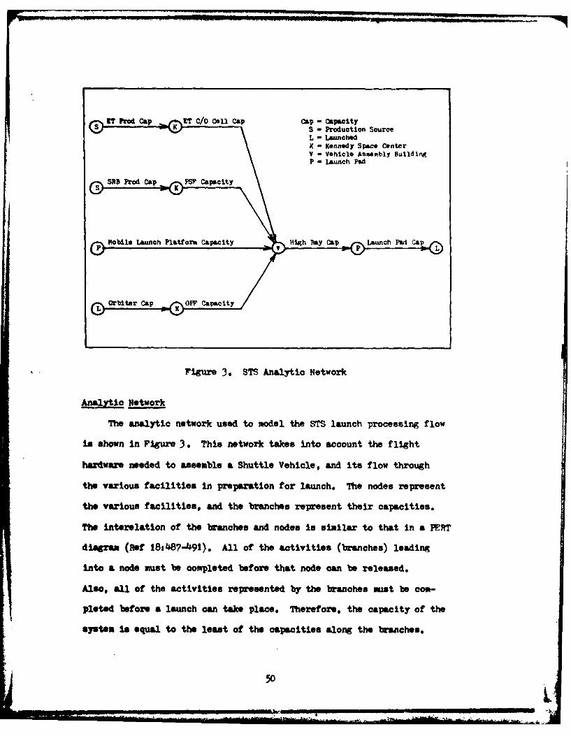
iT iedCap K? o Cll apCap - CapacityS K S - Production Source

L - LaunchedK - Kennedy Space CenterV - Vehicle Assembly BuildingP - Launch Pad

SSR9 Prod Cap KPSP Capacity

PMobile Launch Platform Capacity V High Pay Cap Launch Pad Cap

rigure 3- STS Analytic Network

Analytic Network

The analytic network used to model the STS launch processing flow

Is shown in Figure 3 * This network takes Into account the flight

hardware needed to assemble a Shuttle Vehicle, and its flow through

the various facilities in preparation for launch. The nodes represent

the various facilities, and the branches represent their capacities.

The interelation of the branches and nodes Is similar to that in a PERT

diagram (Ref M~i487-4.91). All of the activities (branches) leading

into a node must be completed before that node an be released.

Also, all of the activities represente" by the branches must be comn-

pleted before a launch an take place. Therefore, the capacity of the

system Is equal to the least of the capacities along the branches,

50

Table I. Activity Times

Activity Time Source*Activity (hours/launch) (Figure #)

MLP Wash 62 14

MLP Refurb 39 14

SRB/ET (Stacking) 272 10

VAB (Orbiter Mating) 168 10

Pad Ope 320 6, 7

Pad Refurb 78 13

T C/O 216 10

PS? Ops 272 11

Orbiter Turnaround Time(Verticle Payload) 80 7

Orbiter Turnaround Time(Iorisontal Payload) 888 6

OFF Time (Vert Payload) 352 7

OW Time (Hor Payload) 400 6

* (STAR 23, Ref 12)Caacities

The capacties of the various facilities are calculated using the

assessed times contained in STAR 23. Since symmetric distributions

were chosen for the simulation model variables, their most likely

values (STAR 23 assessed values) are also their mean values. Therefore,

the use of the assessed values as the expected values of this analytic

approach produces results which can be validly compaed to the simula-

tion results. The activity times contained in Table I were obtained

from Figures 6, 7, 10, 11, 13, and 14 of STAR 23. These times were

used to oompte the capacities of the various facilities and flight

f5

... . .. .. . J " Z illi . i . . . I

hardware. The remainder of this section covers the calculations of

those capacities.

The capacity calculations are dependant on the work week schedule

chosen. The standard work week used is two shifts, five days per

week (2/5). The longer work weeks considered are three shifts, five

days per week (3/5) and three shifts, seven days per week (3/7).

Each shift is eight hours long, and the latter work week, (3/7), is an

around the clock operation. No allowances are made for holidays. The

various activity times are multiplied times a factor which reflects the

work week chosen. This computation determines how many work days are

required to complete an activity. The three work week factors are

calculated as follows,

7 days per work week(0/5) = = o.0875 days/hour (10)

80 hours per work week

7 days per work week(3/5) - 0.0583 days/hour (11)

120 hours per work week

7 days per work week(3/7) - - 0.04'17 days/hour (12)

168 hours per work week

VAD BH y LDcity. In the process of assembling a Shuttle

Vehicle in the VAB, certain hazardous operations take place. During

these operations, the other VAB High Bays are evacuated. Therefore,

the time It taken to assemble a Shuttle Vehicle can be extended by

the requirement to perform hazardous operations in one of the other

High Pays (Ref 127-11). The hazardous operations are Solid Rocket

Rotor (SIM) stacking (52 hours) and Orbiter hoisting (4 hours) (Ref 12).

52

If only one High Bay is used for vehicle assembly, no delays will

result. The expected vehicle assembly time in therefore equal to

(HIP Refurb + SRE/rT + VAB) (13)

or, using the values in Table I,

(39 + 272 168) hours - 479 hours (14)

If two High Bays are used, there is a chance that the hazardous

operations in one bay will delay work in the other. However, if their

operations are running in parallel, no delays will be experienced.

This latter result can occur, since safety constraints do permit the

simultaneous processing of two SRM sets (Ref 12,7-1). The ratio of

hazardous operation time to total assembly time is

56 hoursM 0.117 (15)

479 hours

Assuming the start of assembly operations in the two High Bays are

independent of each other, the probability that operations in one bay

will be delayed by hazardous operations in the other is

1.o - 0.117 - 0.833 (16)

Therefore, the expected assembly time when two High Bays are used is

479 hours 4 (0.883 * ,6 hours) - 528.45 hours (17)

When three High Bays are used for Vehicle Assembly, there will be

at least a 56 hour delay due to the restriction on SRY parallel

processing. A 112 hour delay will result when the three bays operate

53

NIWA O .-- .... .

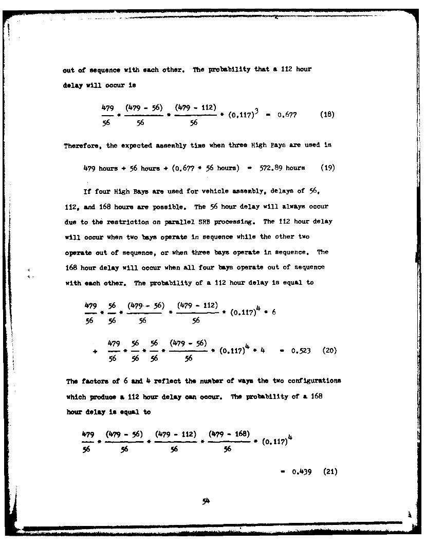
out of sequence with each other. The probability that a 112 hour

delay will occur is

479 (1479 - 56) (1479 - 112)______ * -____ (o.l17) 3 - o.677 (18)

56 56 56

Therefore, the expected assembly time when three High Bays are used is

479 hours + 56 hours + (0.677 * 56 hours) - 572.89 hours (19)

If four High Bays are used for vehicle assembly, delays of 56,

112, and 168 hours are possible. The 56 hour delay will always occur

due to the restriction on parallel SRB processing. The 112 hour delay

will occur when two bays operate in sequence while the other two

operate out of sequence, or when three bays operate in sequence. The

168 hour delay will occur when all four bays operate out of sequence

with each other. The probability of a 112 hour delay is equal to

479 56 (479- 56) (479 - 112) 4- * - * * (0.117) * 656 56 56 56

7956 56 (479- 56)

+ -- *- * (o.117) + * + - 0.523 (20)56 56 56 56

The factors of 6 and 4 reflect the number of ways the two configurations

which pmoduoe a 112 hour delay can occur. The probability of a 168

hour delay is equal to

1+79 (479 - 56) (479 - 112) (49 - 168) 4- *'-.--- *'- *".. (0.117?)

56 56 56 56

-0.1439 (21)

Therefore, the expected assembly time when four High Bays are used is

479 hours + 56 hours + (0.523 * 56 hours) + (0.439 * 112 hours)

- 613.48 hours (22)

The VAB High Bay capacity is computed as

365 days/year* # High Bays (23)

(expected assembly time) * 0.0875

where 0.0875 is the work week factor for the (2/5) schedule. Capacities

reflecting the other work week schedules, (3/5) and (3/7), are computed

using the factors 0.0583 and 0.0417. The capacities for the four VAB

configurations were calculated using Equation 23 and the results of

Equations 14, 17, 19 and 22. These capacities are shown in Table II.

Table II. VAB High Bay Capacity

Work Week Capacity in Launches per Year(shifts/hours) 1 Bay 2 Bays 3 Bays 4 Bays

(2/5) 8.71 15.79 21 84 27.20

(3/5) 13.06 23.68 32.77 40.8o

(3/7) 18.29 33.15 45.87 57.12

55

MLP Capiacity. The MLP caecity is calculate as

365 days/year_________________________________________* # VLPs (21)

(MLP Wash +MLP Refurb + SRB/ET + VAB + Pad Ops) * 0.0875

LP Refurbishment, SRB/ET Stacking, and VAB Obiter mating operations are

carried out in the VAP, while MLP Washing, and Pad Operations are

carried out at the launch pad. If either of these facilities should

go to a (3/5) or (3/7) work week schedule, the equation would change

slightly. For example, the addition of a third shift in the VAB is

calculated as

365 days/year((Wash + Pad) * 0.0875) + ((Refurb + SRB/E:T + VAP) * 0.583)

* M JLPs (25)

Various strategies for increasing MLP capacity were investigated.

Their capacities and their percentage increases over the nominal

capacity (2/5 work week) are shown in Table III. Total YLP capacity

is found by multiplying the chosen strategy by the number of OLPs

available. For example, the three MLPs now available have a nominal

capacity of 3 4 1.85 , or 14.53, launches per year.

56- LJ

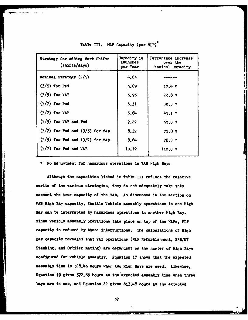
Table III. ?LP Capacity (per MLP)*

Strategy for Adding Work Shifts Capacity in Percentage IncreaseLaunches over the

(shifts/days) per Year Nominal Capacity

Nominal Strategy (2/5) 4.85 ....(3/5) for Pad 5.69 17.4 -9

(3/5) for VAB 5.95 22.8 K

(3/7) for Pad 6.31 30.3 't

(3/7) for VAB 6.84 41.1 f

(3/5) for VAB and Pad 7.27 50.0 1

(3/7) for Pad and (3/5) for VAB 8.32 71.8 %

(3/5) for Pad and (3/7) for VAB 8.64 78.3 ',

(3/7) for Pa an d VAB 10.17 110.0

* No adjustment for hazardous operations in VAB High Bays

Although the capacities listed in Table III reflect the relative

merits of the various strategies, they do not adequately take into

account the true capacity of the VAB, As discussed in the section on

VAD High Bay capacity, Shuttle Vehicle assembly operations in one High

Bay can be interrupted by hazardous operations in another High Bay.

Since vehicle assembly operations take place on top of the YLPs, MLP

capacity is reduced by these interruptions. The calculations of High

Day capacity revealed that VAB operations (14LP Refurbishment, SRB/ET

Stacking, and Orbiter mating) are dependant on the number of High Bays

configured for vehicle assembly. Equation 17 shows that the expected

assembly time is 528.45 hours when two High Bays are used. Likewise,

Equation 19 gives 572.89 hours as the expected assembly time when three

bays are in use, and Equation 22 gives 613.48 hours as the expected

57

time when four bays are in use. The expected time when only one bay is

used is 479 hours. This time is the one that was used to produce the

results shown in Table III. To compute the adjusted values for MLP

capacity, the expected values for High Bay operations were Inserted in

Equation 24 in place of the times represented by (MLP Refurb + SAB/ET

+ TA). The capacities listed in Table IV are these adjusted values.

Total KLP capacity is found by multiplying the listed capacity by the

number of IILPs.

Table IV. !LP capacity

# High Strategy for Adding Work Shifts Capacity ind(shifts/days) Launches

Bays Used (per Year

2 Days (2/5) for VAD and (2/5) for Pad 4.58

(3/5) for VAD and (2/5) for Pad 5.68

(3/5) for VAD and (3/5) for Pad 6.87

(3/7) for VAB and (3/5) for Pad 8.24

(3/?) for VAD and (3/7) for Pad 9.62

3 Pays (3/7) for VAD and (3/?) for Pad 9.17

4 Days (3/7) for VAD and (3/7) for Pad 8.80

* Per ?LP, when two or more High Bays are use

It should be noted from the last three lines above that the

capacity of a single MLP decreases as the number of VAD High Days

used for Shuttle Vehicle assembly is increased. Therefore, an

increase in the number of High Days will force a more than

Woportionate increase in the number of MLPs.

58

* .T C/o ce.ll amity. The ET C/O Cell capacity is computed as

365 days,/ye,,* # C/o Cells (26)

(ET C/o) * 0.0875

The LI C/O time (in hours per launch) was obtained from Table I.

Table V contains the calculated ET C/O Cell capacities for the three

types of work weeks.

Table V. ET C/O Cell Capacity

Work Week Capacity in Launches per Year

(shifts/days) 1 c/o Cell 2 C/O Cells

(2/5) 19.31 38.62

(3/3) 28.97 57.94

(3/7) 4o.56 81.11

* No adjustment for hazardous operations in VAB

However, the capacities in Table V do not allow for work

interruptions caused by hazardous operations in the other VAB High

Bays, Equations 17 and 19 reflect the additional time required to

perform Shuttle Vehicle assembly as hazardous operations periodically

delay High Bay operations. The ratio of ET C/o time to total vehicle

assembly time is

216(27)

479

By multiplying this ratio times the adjusted vehicle assembly times

given by Equations 17 and 19, an expected ET C/O time is obtained.

59

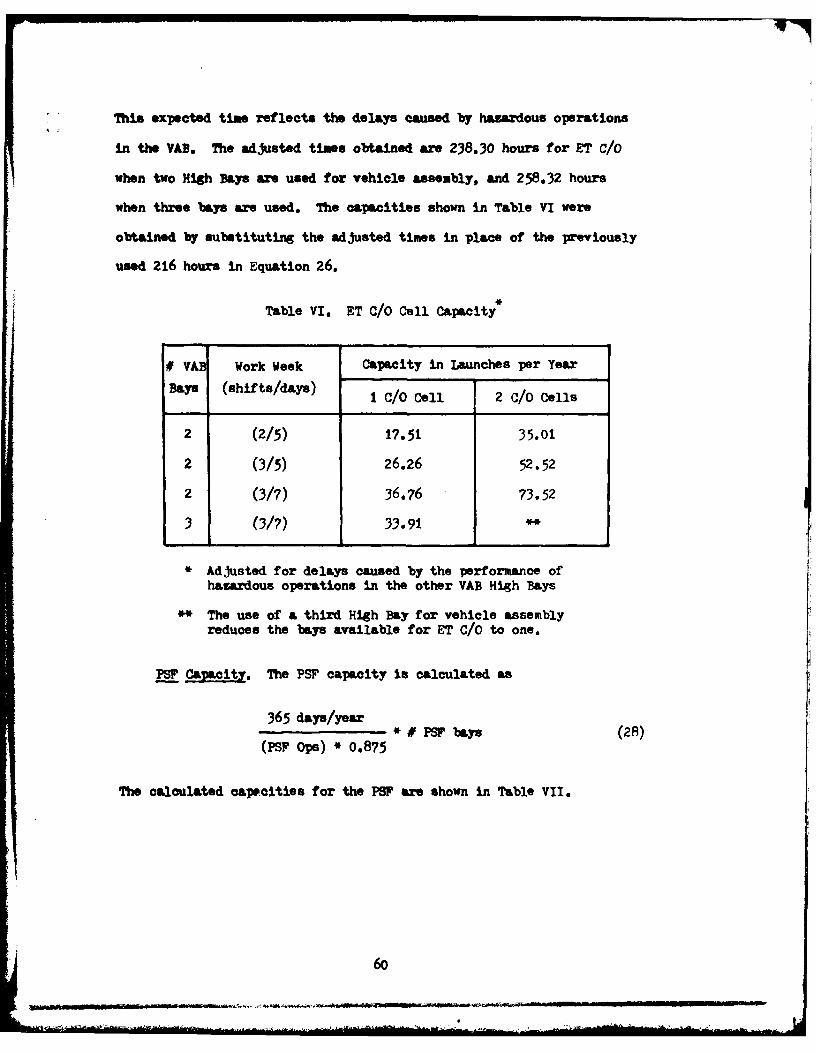
This expected time reflects the delays caused by hazardous operations

in the VAB. The adjusted times obtained are 238.30 hours for ET CIO

when two HiSgh Bays are used for vehicle assembly, and 258.32 hours

when three bays awe used. The capacities shown in Table VI were

obtained by substituting the adjusted times in place of the previously

used 216 hours in Equation 26.

Table VI, ET C/O Cell Capacity

# VAB Work Week Capacity in Launches per Year

Bays (shifts/days) C/O Cell 2 C/O Cells

2 (2/5) 17.51 35.01

2 (3/5) 26.26 52.52

2 (3/7) 36.76 73.52

3 (3/7) 33.91

* Adjusted for delays caused by the performance ofhazardous operations in the other VAB High Bays

The use of a third High Bay for vehicle assemblyreduces the bays available for ET C/O to one.

P X aacity. The PS7 capacity is calculated as

365 days/year*# P bays (28)

(PSi Ope) * 0.875

The calculated capecities for the PSP are shown in Table VII.

60

Table VII. PS Capacity

Work Week Capacity in Launches per Year

(shifts/days) I PS? Bay 2 PS? Bays

(2/5) 1534 30.67

(3/5) 23.00 46.o1

(3/7) 32.21 64.41

Orbiter Capacity. The Orbiter capacity computation is made under

the assumption that all ground operations take place on an around the

clock basis (3/7 work week). This action enables Orbiter capacity

limitations to be identified separately from facility limitations.

The equation for computing Orbiter capacity is

365 days/year..... .. * A' Orbiters (29)

(Expected Turnaround Time 4 Expected Flight Time)

The current flight manifest shows that approximately 51.74 of the

missions will require payload installation in the OP! (Ref 9). This

activity increases the overall turnaround time by 48 hours to 888 hours.

The rest of the missions (48.3%) will have their payloads inserted at

the launoh pad, and the assessed turnaround time for these missions is

84O hours (Ref Table I). The expected Orbiter turnaround time thus

becomes

(888 hours * 0.517) + (840 hours * 0.483) - 864.82 hours (30)

or

(864.82 hours * 0.0417 days/hour) - 36.034 days/launch (31)

61

The expected flight time is computed using the flight time distribu-

tions assumed for the simulation model. Those were normal distribu-

tions with means of 12 days for Spacelab missions and 4 days for all

others. The relative percentages for the two were based on the current

flight manifest and are 17.2% and 82.8%. Therefore, the expected

flight duration time is

(12 * 0.172) + (4 * 0.828) - 5.38 days/flight (32)

By plugging the results of Equations 31 and 32 into Equation 29, the

computation of Orbiter capacity becomes

365 days/year* 0 Orbiters (33)

(36.03 days/launch + 5.38 days/flight)

Orbiter capacity for various numbers of Orbiters is shown in Table

VIII. An additional Orbiter is included for VAFB operations.

Table VIII. Orbiter Capacity

. Capacity in# Orbiters Launches

per Year

2 8.81

3 17.63

4 26.44

5 35.26

6 4 4.07

7 52.89

8 61.70

* Includes one Orbiter for VAPB

62

However, separate computations which take into account the work

weeks used in the OF, VAP, ad on the launch pad were made. The

capacities obtained were used in conjunction with the launch enhancement

plan to show the need to -uickly go to (3/7) work week schedules in the

three facilities, The computatilons to cahaate the capacities are

similar to those used in computing MLP capacity. For example, Orbiter

capacity with OP, VAB, and Pad times of 376.82 (Equation 37 result),

168, and 320 hours, and a (3/5) work week, is

365 days/year-* N Orbiters(3)

((376.82 + 168 + 320) * 0.0583) + 5.376 days/flight

An additional corTection was made while doing these computations. In

the section on VAP High Pay capacity, it was shown that hazardous

operations in one High Bay can delay normal operations In the others.

The mating of an Orbiter to an ET/SRB assembly is one of the operations

which can be interrupted. The number of High Bays used for vehicle

assembly affects the expected delay. Equations 17, 19, and 22 take

into account this delay and can be used to recompute the time it takes

to route an Orbiter through the VAL. The ratio of Orbiter mating time

to total vehicle assembly time is

168(35)

4179

Equation 17 gives the adjusted assembly time as 528. 4 5 hours when two

High Days are used. For the use of three bays, Equation 19 gives

5?2.89 hours as the adjusted time. Finally, Equation 22 gives a time of

613.48 hours as the adjusted time when four bays are used for vehicle

63

assembly. By multiplying these numbers times the ratio in Equation 35,

expected times for Orbiter VAB operations can be obtained. The calk

lated values are 185.32 hours when two bays are used, 200.93 hours

when three bays are used, and 215.17 hours when four bays are used.

These values are used in place of 168 hours in Equation 34 to obtain

the results shown In Table IX.

Table IX. Orbiter Capacity

Work Week Orbiter Capacity in Launches per Year"4

O1P VAB Pad 2 Orbiters 4 Orbiters 5 Orbiters 6 Orbiters

(2/5) f2/5) (2/5) 4.42 13.26 17.68 22.10

(2/5) ?3/5) (2/5) 4.73 14.19 18.92 23.65

(2/5) f/5) (3/5) 5.38 16.14 21,53 26.91

(3/5) 3/5) (2/5) 5.52 16.55 22.07 27.58

(3/15) 3/5) (3/5) 6.42 19.27 25.69 32.11

(3/5) f3/5) (3/7) 7.09 21.26 28.35 35.44

(3/7) b/5) (3/5) 7.22 21.66 28.88 36.10

(3/7) f3/7) (3/5) 7.69 23.07 30.76 38,1.5

(3/7) f3/7) (3/?) 8.66 25.99 34.65 43.32

(3/7) ?3/7) (3/7) 8.53 25.60 34.13 42.66

(3/7) 3/?) (3/7) 8.41 25.25 33.66 42.08

* The number in the upper left corner of each VAB entry Is thenumber of VAB High Bays used for Shuttle Vehicle assembly.

Includes one Orbiter for VAI'B operations

64

. ... . .. -. . . . .. .I : _.? ,, + - . . . . . . . . . . . . . . .. . . . . .. . .. . . .- -- +--

OPP Capacity. The capacity of the O1 Is dependant on the work

week schedule, The equation for computing OPP capacity (assuming a

(2/5) work week schedule) is

365 dayB/yer,*N#opF"bay (36)(oPP time) * 0.0875

Missions requiring payload insertion in the OPP extend O1 time to 400

hours. The OWP time for all other missions is 352 hours and the rela-

tive percentages of the two types of missions are 51.7% and 48.31

(Ref 9). Therefore, the expected OW time is

(400 hours * 0.517) + (352 hours * 0.483) - 376.82 hours/launch (37)

This time was used in Equation 36 to produce the results shown in

Table X.

Table X. OFF Capacity

Work Week Capacity in Launches per Year

(shifts/days) 1 Bay 2 Bays 3 Bays

(2/5) 11.07 22,.14 33.21

(3/5) 16.61 33.21 49.82

(3/?) 23.25 46.50 69.74

65

Launch Pad Caaity. The equation for computing the launch pad

capacity is

365 days/year36 - * # launch pads (38)

(Pad Ops + Pad Refurb) * 0.0875

Using the activity times listed in Table I, the various launch pad

capacities were computed. These results are presented in Table XI.

Table XI. Launch Pad Capacity

Work Week Capacity in Launches per Year

(shifte/days) I Pad 2 Pads 3 Pads

(2/5) 1O.48 20.96 31.44

(3/5) 15.72 31.44 47.16

(3/7) 22.01 44.02 66.03

IT and SRB Capaoities. The ET and SRB production rates are

building towards 24 per year. Their production facilities are designed

to allow the implacement of the additional equipment needed to bring

their production rates to 40 per year. A greater effort would be

required to increase the production rates beyond 40 per year (Refs 221

23l and 24), This analytic approach assumes that the ET and SRB

production rates are increased to the levels needed to meet the desired

launch rates.

Launch Enhancement Plan

Tables II through XI were used in conjunction with the network

shown in Figure 3 to develop the launch enhancement plan shown in

66

Table XII. At each step in the development of the plan, the facility

or hardware with the least Capacity was identified and capacity added

to it. The process for adding capacity was to add work shifts before

adding facilities. This process assumes that available resources will

be fully utilized before additional facilities are constructed. The

first line of the plan gives the current capacity of the STS at KSC.

This capacity is based on the completion of current construction plans

and includess

1. 14 shuttle Orbiters (one of which is dedicated to VAFB),

2. 20PP bays,

3. 2 VAP High Bays (out of the 4 High ays in the VAB),

4. 1 PS? bay (this facility also contains two storage bays),

5. 2 ET C/O Cells (positioned in two of the VAB High Pays),

6. 2 Launch Pads, and

. MLPs (assuming the third available MLP is reconfigured for

STS use).

The configurations and capacities of each of these facilities and

hardware are shown in the columns below the appropriate headings on

Table X1I. The first entry in each cell gives the units needed (bays,

HIPs, eto) to produce the associated capacity. The second entry gives

the work week schedule employed (if appropriate) and the lower entry

gives the capacity of that configuration. The capacity for the over-

all configuration represented by a row in the Table is given in the

left hand column. This overall capacity is found by locating the

facility or hardware on that line which has the least capacity. The

second column gives the corresponding capacity obtained from the

simulation approach. To use the plan, locate the entry in the left

67

hand column which corresponds to the desired launch rate, and read off

the configuration needed from the other columns in that row.

As can be seen by comparing the first two columns, the simulation

results closely match the analytic results. The sequencing of facility

and hardware additions are about the same and the corresponding launch

rates are nearly equal. Therefore, the simulation results appear to be

valid. This final step in the validations process greatly increases the

confidence with which the more accurate simulation method and results

can be used. However, the analytic method proved to be more accurate

than expected. Therefore, it may be good enough to use in those

situations where less accuracy is acceptable. At any rate, the analytic

method should be used in conjunction with the simulation method when the

latter method is chosen to insure the simulation results appear valid.

Since two of the four VAB High Bays are used for ET C/O and

storage, an increase in the number of VAB High Bays used for Shuttle

Vehicle assembly will cause a decrean in the number of ET C/o Cells.

This result will create the need for the construction of a separate

ET C/O and storage facility.

68

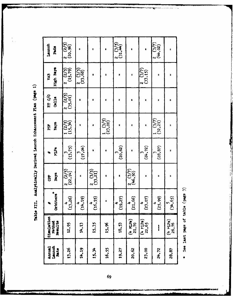
0% U"NU4 cnO M"

N l C-4

NN

0 ul N N

00a

U-4 NON

NO 0% ~ - \C -

~~ N N -* -

-4 %- -4-4

0l

"-4 - C-

00 N ~ (. O

s- Ii N I 'N~ '4 'N'*U

69...

C--m M4CD-

NY

0 '

61 __-4_

-'4

0' w0 C- 0

4 to--f 9 4-65 OD NOoH

4:0 (Nj.

414(n4 \C) 6

9-4%

9-40

0 40S

4J ~ w4 4)W4O w 6 44 4-) 4U. (r- $ r4 ON 0 P

4 4r4to

.4w * P4 4 4 .

0E-C: oWNV 4) )A

04X -, *4 +m 4-4

~v p

- -) -- - -*U 4J

v- CCa 0 -

'Zl* 0 4 441 x x a0 ) 04

0 0 E-kk 43 )'0)

-c'.44 -0 am 0k 4

- -- 0 44 )4) -P " . i k 4 ) " 1

VI. Application and Analysis

This chapter presents the applications and analyses of the simul-

ation models described in Chapter III. In addition, the results of the

sensitivity analysis conducted on the moels is presented. The first

section describes the results of the sensitivity analysis conducted on

the VAFB model and the final results obtained from the model. The

methodology used to incorporate the VAF3 results into the KSC model is

also presented. The second section of this chapter presents the

analysis of the KSC model. This section includes the results of the

various sensitivity analyses conducted, a sample analysis of the output

from the model including a statistical testing of the results, and the

final results obtained from the analysis of the KSC simulation model.

VAFB Model Analysis

Sensitivity Analysis. As mentioned in Chapter III, little

information was available on which to base the determination of the

type of distribution to use for the process times at VAFP. This

situation was mainly due to the fact that no actual data exists to

compare the times to. For the reasons stated in Chapter III, the normal

distribution was selected as the distribution to use for this model.

However, two other possible parametric models were considered and

sensitivity analysis was conducted to determine how the use of the other

models would affect the outcome of the study. The two other methods for

modeling the times were, one, to use the uniform distribution, and, two,

to use constant times, For the uniform distribution model, the allotted

and assessed times from VSTAR 05 were used as the endpoints of the

distribution. If the allotted and assessed times were identical, a

72

LM-

constant time was used. In the constant time model, the maximum of the

allotted or assessed times was used as the time for the activity. In

both of these models, the distributions and the times for ET shipping

and Orbiter mission were the same as those in the normal mode. The

results from these models is presented in Table XIII.

Table XIII. Three VAFB Distribution Yodels

Mean Time Standard AnnualBetween Launches Deviation Launch

Rate

Normal 32.3551 0.1689 11.281

Uniform 31.8657 0.1374 11.454

Constant 34.3691 0.1171 10.620

These results were tested to determine if there was a significant

difference between the launch rates obtained from the three models.

Since the normal model was the model selected for use, the other two

models were compared to the results of this model. In this test, the

null hypothesis is that the means of the two models being tested are

equal, hile the alternative hypothesis is that the means are not equal.

For this test, the assumption is made that the means are normally

distributed. The Central Limit Theorem indicates that this assumption

is valid for distribution which are the sum of many independant,

identically .istributed functions (Ref 30). This is the case here.

The test statistics and the methodology for applying these tests is

that whioh was presented in Chapter III.

Flrst, the equality of the variances was determined. The statis-

tic that the test statistic was compared to is found in Equation .3 of

73

Chapter III. If the test statistic was greater than this value, the

variances were not considered equal. If the test statistic was less

than 4.03, the variances were considered equal. For the normal versus

uniform model, the test statistic was F° - (0.1689)2/(0.1374)2

- 1.51 and thus the variances of these two models were considered

to be equal. For the normal versus constant model, the test statistic

was FO - (0.1689) 2/(0.1171)2 - 2.03 and the variances of these

two models were also considered to be equal.

Since the variances are equal in these cases, the test statistic to

use to test the equality of the means is that of Equation 4 in Chapter

III, This test statistic requires the calculation of S usingP

Equation 5. The test statistic in this case is compared to the

following statistic

"9/2. n, + "2- 2 (39)

If the absolute value of the test statistic is greater than the

statistic calculated using Equation 39, the means are considered to not

be equal# otherwise they are considered to be equal. In these cases,

the value for at is 0.05 and n I , n2 - 10 , and thus the value of

thp statistic in Equation 39 is 2.101 (Ref 30,600). For the normal

versus the uniform model, the value for Sp is 0.1532 and t o is 7.145.

Therefore, there is a significant difference between the two models.

For the normal versus the constant model, S is 0.1430 and t isp 0

-31.4W6. Therefore, there is also a significant difference between

these two models. This analysis reveals that the distribution chosen

does Indeed have an effect on the outcome of the model. However, the

difference in launch rates (Table X1I) is not significant from a

74L

practical point of view. Thus the selection of the normal distri-

bution is reasonable and, If fact, results in a mean launch rate that

is nearly midway between the launch rates of the other two models.

The results are assumed to be more sensitive to the times used in the

distribution than to the actual distribution chosen. Therefore, an

significant changes in the projected times for the activities modeled

could have a greater affect on the outcome.

Model Results. The VAFB model was run with both one and two

Orbiters dedicated to the facility. The results of these runs are

shown in Table XIII.

Table XIII. VAFB Model Results

Number of Mean Time Average AnnualBetween Launches Launch Rate

Orbiters (days) (launches/year)

1 32.3551 11.281

2 19.,411? 18.797

Various sources (Rob 31,23 and 33t6) indicate that the average number

of laundes out of TAF3 will be out 10 per year. Thus with the assessed

times used in this model, the expected launch rate could be achieved

with only one Orbiter, while the maximum rate of 20 per year that was

forecast in the initial studies could be nearly reached with two

Orbiters dedicated to VAF use (Ref 21s1).

Since the expected rate of launch from VAPB is 10 per year, it was

decided that this value should be used as the annual launch rate for

VAP in the XSC model. It was decided that these launches should be

uniformally distributed throughout the year, since this is the

75

_ -_ l l I ' I l B i _- i

assumption made for the VAFB launches in VSTAR 05.

The distribution used in the KSC model for the processing time of

the Orbiter at VAFB was determined simply by using the results of the

VAFB model directly. In addition, it was decided not to dedicate an

Orbiter to VAFB in the KSC model due to the fact that this would result

in the Orbiter remaining idle at VAFB for part of the year when that

Orbiter could be put to use at KSC. Therefore, the KSC model allows

any of the Orbiters to be launched from VAFB. However, if the launch

rate at VAFB increased to 11 or 12 per year, it would be necessary to

dedicate at least one Orbiter to VAFB. Additionally, if the processing

time for VAFB increases any great amount, then an Orbiter would have

to be dedicated to VAFB.

KSC Model Analysis

This section presents the analysis of the KSC simulation model.

First, the results of the sensitivity analysis conducted on the distri-

butions, length of each run, number of runs to determine a data point,

and the payload mix probabilities are presented. These results are

followed by a ample analysis of the output from the model including the

statistical testing of the results. Finally, the results of the analysis

using the KSC model are presented.

Sensitivity Analysis. The first concern of this analysis, as

mentioned in Chapter III, was the degree to which the optimistic and

pessimistic times chosen for the beta-PERT distribution affected the

results. To analyze this, the model was evaluated under four

conditions, with the endpoints for the distribution changed each time.

For the first case, the optimistic time was taken as the allotted time

and the pessimistic time was set so as to make the distribution symmetric

76

around the most likely time. In the second case, the pessimistic time

was reduced so that the distance between the pessimistic and most likely

time was one third the distance between the optimistic and most likely

time. The third case returned the value of the pessimistic time to that

it originally had and set the optimistic time so that it was one third

of its original distance away from the most likely time. Finally, in

the last case, the optimistic and pessimistic times were both moved to

the one third points used in the preceeding two runs. All runs were

3650 days in length and each result was based on 10 repetitions. The

results of these runs are presented in Table XIV.

Table XIV. Distribution Changes Results

Case Number Days Between Standard AnnualLaunch-

Launches Deviation Rate

1 28.1827 0.506i 12.951

2 25.7959 O. 1698 14.146

3 29.8880 0.4821 12.212

4 27.0461 0.1592 13.495

For the test of the variances, the test statistic used is in

Equation 1 from Chapter III and this statistic is compared to the value

given in Equation 3. Th null hypoth is is that the variances are equal,

while the alternate hypothesis Is that they are not equal. The results

of these tests are presented in Table XV.

77

* •Table XV. Test on Distribution Cases Variances

Cases

Compared F 0 Results

I vs 2 8.892 cr2 4 '1 2

1 vs 3 1.102 O*2 . Q2

1 3

I vs 4 10.123 o'2 G- 21 4

The next step was to test the equality of the means. The null

hypothesis is that the means are equal, while the alternate hypothesis

is that they are not equal. For the cases where the variances were found

to be unequal, the test statistic used was that in Equation 8 and this

statistic was compared to t,2 ' v where v is calculate according to

Equation 9. For the case where the variances are considered to be equal,

the teat statistic is that from Equation 4 with Sp calculated as in

Equation 5. This is compared to /2, nI + n 2 * The results of

this analysis is presented in Table XVI.

Talbe XVI. Tests of Distribution Means

Casest 0 ResultsCompared0

I vs 2 14.2283 u1 # u2

t vs 3 -. 716 uI # u3

1 vs 4 6.7?6 u1 U u4

78

Therefore, the endpointa chosen for the distribution do have an

affect on the output of the model in terms of time between launches.

However, the calculated launch rates are not drastically different

(Table XIV). Thus, there is some possible error due to the endpoints

chosen. However, by using the endpoints chosen in the paranetric model,

the overall model allowed for both unexpected delays and time reductions

in activities. This fact, along with the reasons cited in Chapter III,

resulted in the choice of the endpoints in case I for use in the model.

Next, it needed to be determined whether or not the length of the

runs (3650 days) was adequate to characterize the mean time between

launches. To test this length, the model was run for both 3650 and

7300 days. The results of these runs are presented in Table XVII.

Table XVII. Run Results

Time Bqetween StandardLength of Run

Launches Deviation

3650 days 28.1827 o.5061

7300 days 28.2833 0.2598

First, the equality of the variances was checked using the

formulas in Equations 1 and 3. In this case, F° - 3.794 which is

less than 4.03 and thus the variances are considered equal. The means

are compared uslig Equation 4 for the test statistic and t/2, n + n 2

for the comparison statistic. To calculate to, Sp must first be calcu-

lated using Equation 5. For this example, SP - 0.38295 and

to -0.587 . The absolute value of t is less than t0. 0 2 5 , 10 or

2.101. Therefore, the meas we not significantly different and 3650

79

II I_ I ] - . . . -- I I = -- - -- I ...

rdays is an adequate run length for characterizing the mean time betweenlaunches,

The next area that required testing was that of the number of runs

required to adequately characterize the mean. For this analysis, three

different values for the number of runs were examinedl these being 5

runse, 10 runs, and 50 runs. Each run was 3650 days in length as

determined before. The results of these different cases are presented

in Table XVIII.

Table XVIII. Number of Runs

Number of Runs Time Between Standard

Launches Deviation

5 28.1008 0.5919

10 28.1827 0.,061

50 28.2596 0.14152

The variances and means um tested as in previous analyses. The results

are presented in Tables XIX and XX.

Table XIX. Thst on Run Variances

Runs Compared l0 Result

10 ve 5 1.368 2 ao10 5to v 5 .: 8 2 - "2

10 ,. 50 2.4 02 "10 95

80!

-- _ " ... I II III I I IIII _ [ 2 -

Table XX. Test on Run Means

Cases Compared t Result0

10 vs 5 0.2800 uto - u 5

10 vs 50 -0.5155 u 1 0 " U50

Therefore, there Is no statistically significant difference

between 5, 10, and 50 runs of the system. They all characterize the

mean well. Ten runs was chosen for the model since fewer runs

would decrease our confidence in the results, and more runs would

have increased the computer time required to complete a simulation

run,

Finally, the probabilities that were selected to determine the

type of payload to be placed in the Orbiter were examined for their

affect on the results. There are two places in the model where the

payload type could affect the turnaround time. They are the OP

payload activities and the mission flight times. In the OPP, horizontal

and Spacelab payloads (types 1 and 2) require more processing time

then do the verticle payloads (type 3) which are loaded at the pad.

This difference is expected to have little effect though, since

regardless of the payload type, the same maintenance activitits are

performed. The mission duration, however, could affect turnaround.

The Spacelab mission has an average duration of 12 days, while the

other missions have an average duration of only 4 days. Therefore,

significant increases in the number of Spacelab missions could

increase the turnaround time for the Orbiters, To test the

81

sensitivity of the model to the payload types the following payload

variations were tested (Table XXI).

Table XXI. Payload Types and Probabilities

Payload Type 1 Payload Type 2 Payload Type 3Payload Case Probability Probability Probability

1 0.172 0.345 0.483

2 0.1 o.4 0.5

3 0.2 0.1 0.7

4 0.3 0.2 0.5

5 0.5 0.1 0.4

The results from each of these cases is presented in Table XXII.

Table XXII. Payload Type Tests

Days Between StandardPayload Case Launches Deviation

28.1827 o.5o61

2 28.1101 0.3559

3 28.2174 0.20?0

4 28.5976 o.2476

5 28.5791 0.2779

These results were tested using the same methodology given in the

Wevious analysis. The results of these tests are contained in Tables

XXII ad XxIv.

82

Table XXIII. Test of Payload Variances

Payload Case F Results0

I vs 2 2.022 o,2 -( 2

1 &

I vs 3 5.978 Cr C(#

1vs4 4.178 1 2 0 42

1 vs 5 3.317 O I2 21 5

Table XXIV. Test of Payload Means

Payload Case t Results

I vs 2 0.377 u1 " u2

I vs 3 -0.201 u1 - u3

1 vs4 -2.329 u1 4 u4

I vs 5 -2.261 uI ' u5

The above results indicate that as the percent of Spacelab

payloads increases, the greater is the effect on the model results.

However, no effect was significant until the Spacelab made up 30

percent of the total payloads. A review of the current flight

manifest indicates that the probability of Spacelab use being this

high Is low, and therefore this concern is not a major one (Ref 9).

83

Sample Analysis and Results. The following is a stp by step

analysis of the output from the Q-GERT model. The output from the

starting configuration is used for this example. The sample output

used can be found in Figures 4 and 5. The calculations shown are

representative of the calculations used throughout the analysis.

The first step is to determine the launch rate that the current

configuration is capable of achievinr. This is accomplished by using

the average value (column headed by AVE.) for node 40, LAUNCH. This

number is the average time between launches, which in this case is

28.1827 days. The launch rate is found by dividing this number into

365 days per year. This calculation yields a launch rate of 12.951

launches per year.

Once the launch rate has been calculated, the next step is to

determine the factor(s) that is/are limiting the launch rate. This

job is done by first looking at the Average Resource Utilization and

Availability tables of the output (Figures 4 and 5). These tables

indicate that the PSF, VAP, FT Parge, FT checkout cell, ET storage

cell, and the SRP storage are all in nearly constant usp. The fact

that the SRB storage and the FT storage cells are nearly full indicates

that the functions filling these cells are producing above the level

required and as such they are not the limiting factors. This step

eliminates the FT production and the PSF from consideration as limiting

factors. This step also indicated that the VAB may be a limiting factor.

The next area of the output to examine is the queue node statis-

tics. The data in the queue table can be used to determine where items

are waiting in queues and the length of time that they are required to

wait. The following nodes are of the most interest for this analysis,

84

AD-A124 706 AN ANALYSIS OF THE SPACE TRANSPORTATION SYST EM LAUNCH /PAT P CAPABI TY UT. (U) AI F ORCE INS 0F TCHWRIGHT-PATTERSON AFB OH S CHOO LOF ENGI.

UNCLASSIFIED J ANDRUSYSZYN ET AL. D SFG92 N

IIIIIIIIIEIEIIIIIIIIIIIIlIIIIIIEIIIIIEEEllllihhhm

IEEE':

16 L

1. L L811111125 1.4 Q6

MICROCOPY RESOLUTION TEST CHARTNATIONAL BUREAU OF STANDARDS-1963-A

Coco-

c* im 00 00 9.0 00 0 00, a0 0

.1 w 0 a IW, '" 00. C. 20 ai.O N .O

I-h

-hi 33U'0 3U

-.4-

-i . . . . . . ..

16.... ..

hi 0 0 00,0 010 4

-- t . .1 4 -ft - " t0

-- --- - - Nn o o r0-...... N.va 0

cv, ~~~~~~~~~. . . . . . . . .. . .i * m a w .. y r 0 .- ~ fra

,o VMS

*~~~c eel w*~f I.if Nm .tVZi aW1oo -

* - S -85

W~ I- IOn.v

Ie . to in

* ao

12U

0 42000 0. 1

oc

.. i~~~ C, r.. 0- * * *

a 64 V. w

0 me

*Z 00 1" 000

if~3 . . .. u . i. .

o ~ ~ ~ ~ ~~1 00 if i 0iCWNe i .r0C

IL en L*Wf 00 .b.

-9 4W4.4ifif:!fO@ i

a af 0 @~ --0c~l- mo l0

hi P 0 if CS - 00 L,

b* a%* * * ~ - S *

* 43 O~wo p 0 C 86

* . 1. Node 2, WAITOP - Orbiters wait in this node for an Opp bay,

2. Node 27, ORBWAIT - Orbiter waits for SRB/ET assembly after

finishing processing in the OPI

3. Node 78, WAITrmD - the ET/SRB assembly waits for an Orbiter to

finish OFF processingg

4. Node 58, WAITSTOR - SRB set waits for SRP storage cell;

5. Node 63, WAITML - SRB set waits in storage for MI/VAP High

Bay to become availablel

6. Node 68, WAITSRB - the 1 L/VAB waits for an SRB set;

7. Node 65, WAITVAB - the MLP waits for a VAM High Bayl

8. Node 72, WAITET - the stacked SRB waits for an ET; and

9. Node 94, WAITSRB - the ET waits for the stacked SRB set,

The two columns of primary interest in this section of the output

are the average number in the queue node and the average waiting time in

the queue. The average waiting time is calculated based only on the

transactions that actually have to wait.

The best method of analysis of the queue data is to compare the

data for queue nodes that proceed an assembly operation. As a starting

point, the data on the Orbiter waiting to be mated (node 2?) and the

data on the ET/SRB assembly (node 78) are compared. The information

in the output indicates that there is a larger average number of Orbiters

waiting (0.2632) as compared with the average number of SRB/_ET assemblies

(0.0829). In addition, the Orbiters wait longer (7.4110 versus 2.3464

days) than the SRB/FT assemblies. These results indicate that neither

the OPP nor the Orbiters are the limiting factor, bat that the delay is

ooouitft prior to the SRB/FT mating operation. The first assembly point

prior to the SRB/RT mate indioated that the SRB Is not waiting for Fs

87

4 (node 72). The ETa on the other hand wait in storage an average of

55.6275 days (node 94). This time appears excessive. .iowever, it is

primarily due to a slight over production of ETs.

The next point where components wait for assembly is prior to the

SRB stacking. The queues before this point indicate that there is an

average of 1.8484 SRBs waiting (node 63) while the YLP/VAB never have to

wait for an SRB set. This difference Indicates, as did the resource

data, that the PS? is processing an adequate number of SRPs and it is

not the limiting factor.

The analysis so far has narrowed the limiting factor down to either

the YLP or the VAB. The data for queue node 65 indicates that there is

an average of 0.1302 MLPs waiting an average of 3.6870 days each for a

VAB bay to become available. This leads to the result that the VABs are

the limiting factor. This fact agrees with the data in the resource

tables discussed previously. Keeping in line with the philosophy stated

in Chapter III, shifts are added to the VABs before a new VAR High Bay

is added. At this point, the work shifts in the VAB were increased from

two shifts for five days per week to three shifts per five days per week.

The model was then rerun and the result was an average time between

launches of 25.8320 days and a launch rate of 14.129 launches per year.

To determine if this is a statistically significant increase in the

launch rate, the statistical tests described in Chapter III were

accomplished. The sample calculations for these tests is presented in

the following paragraphs.

he average time between launches for the first run was 28.1827 days

and the standard deviation was 0.5061. Por run two, the average time

between launches was 25.8320 days and the standard deviation was

88

0.2060 days. The first step was to test the equality of the variances.P was found to be 6.036. This is larger than the comparison statistic

0

(4.03) and therefore the null hypothesis is rejected and the variances

are assumed to be not equal.

Next, the null hypothesis of u1 - u2 was tested against the

alternate hypothesis that u1 > u2 . The test statistic in this case

was found to be 13.598. The comparison statistic is tA, v whereV[

v - 12.548 . Therefore, the value of the comparison statistic is

1.771 (Ref 30:596) at at - 0.05 . Since to is greater than the

comparison statistic, the null hypothesis is rejected and the time

between launches for the first run is assumed to be greater than that

of the second run, This leads to the conclusion that the launch rate of

the second run is greater than that of the first run.

At this point, the output of the second run was analyzed to deter-

nine the limiting factor. This process was continued until the desired

launch rate was achieved. The results are presented in Table XXV.

The results in this table show the facility additions that this study

recommends and the order in which they should be added to efficiently

increase the launch rate. There were some instances where the analysis

of the output indicated that there were two or more limiting factors

occurring at the same tine. In these cases, each of the limiting

factors were increased individually to determine which factor increase

would result in the greatest increase in launch rate. 'A table presenting

al of the oonfigurations examined can be found in Appendix A.

89

Table XXV. Simulation Derived Launch Enhancement Plan

Launch/ YP aucWae Ories Days IILPU Bap 0*3ls Hg Days Pads

12.95 14 2 (2/5) 3 1 (2/5) 2 (2/5) 2 (2/5) 2 (2/5)

14.13 a 1 of So 2 (3/5)

15 .35 2 (315) "

15.96 " 1 (3/5) " " "

18.53 - to 2 (3/5)

21.70 2 (3/?) 4 " " I "

22.65 o " " IS 2 (3/?)

24.0 98 01 (3/?) " No

26.76 2(3/?)

3o.o6 5 " " 2 (3/5) o of

31.34 ot/ 2 O 3 (3/?)

32.68 o S 2 (3/?) " " "

33146 6 " " " " "

37.42 "5 o of o

38.95 14(3/7)

40.20 3 (3/?) " S " So

41.614 tf6

43.68 7 It f " t

48,16 Soof 3 (3/?)-em - -.. - - - -. - -307

I noludes one Orbiter for VAP operatios

** The addition of the third HSgh Day for vehicle assembly reduces thenumber of ZT 0/0 Oells in the TAB to one. As this single cell cannot handle the launch rate, a separate, two cell ET C/a and storagefacility wil have to be built.

See the next pege for additional comments on this plan.

90v

Additional comments on the Enhancement Plant

1, The PSI' has two storage bays In addtion to the single processingba,. The addition of a second PSI is required when the launchrate reaches 30.06 launches per year. This second facility wasrun with a single proessing bay and three storage bays. Thetotal of the two PS' facilities is then two processing baysand five storage bays.

2. ST and SRP production rates are assumed to match the annuallaunch rate. This annual launch rate includes the rate forKSC and that for VAFB (assumed to be 10 per year). Therefore,it should be Increased to 40 per year when KSC reaches 14 peryear, and to 60 per year when KSC reaches 30 launches per year.

3. The simulation results showed that a single crawler (of the twoavailable) was sufficient to handle all the launch ratesexamined. In addition, four barges able to handle a single ETeach were found to be able to handle all of the launch ratesexamined. The model assumed that there was an additional, fourST barge available to transport ITs to VAPD.

4. The model also assumed that there were as many ET storage cellsas there were C/o cells.

91

rVII° Conclusions

The Space Transportation System is being developed to launch

USA, DoD, and commercial payloads. National policy directs NASA and

DOD to use the STS as their primary means for launching payloads into

earth orbit. Consequently, most DoD payloads will be launched by the

STS, and DoD's share of STS flights will rise to 50% after 1988.

Scheduled DoD panoads include missile warnlng, surveillance, communi-

cation, navigational, and meterological satellites (Refs 11 and 2).

Future payloads may include space based defensive weapon systems

(Refs 3,151 4tl).

Unfortunately, STS launch capacity is already saturated, and the

flight hardware procurement and launch processing facility construction

needed to increase the system launch rate are not contained in current

fundin plans (Refs 5 201 and 6s16-17). Those funds which may later

become available must be wisely spent to insure that the launch rate is

increased to the level needed to meet critical national defense needs.

Therefore, they must be spent on those portions of the system which

contibute greatest to increasing the system launch rate.

The purpose of this thesis effort was to develop a plan for

increasing the STS launch rate. The problem was to develop a method

to accurately predict STS launch rate capability given various facility

configurations and flight hardware levels. Two such methods were

developedl one rres an analytic approach, while the other uses a

simulation approach, The analytic approach in Chapter V turned out

to be surprisingly useful. However, it does not accurately reflect

the complex interactions which occur as flight hardware progresses

thaough the launch processing facilities. The simulation approach

uses Q-GNRT modeling techniques to properly reflect the flow of flight

hardware through the various facilities, and the complex interactions

which result. Both methods properly identified the bottlenecks in the

STS and were used to develop plans for sequentially adding capacity at

bottlenecks in order to efficiently increase the system launch rate.

These plans are based on the assumption that work shifts will be

adddd at the processing facilities before the facilities are expanded

or additional flight hardware is procured,

The times it takes to complete the various processing activities

were obtained from the S Shuttle Turnaround AnalyisR

(STAR 23) (Ref 12). Only five STS launches have taken place to date,

and the processing activities are still high on their learning curves.

Consequently, the available samples of activity times are not adequate

for use in determining their ultimate statistical distributions.

Therefore, the assessed activity times given in the STAR are the best

available estimates of the times to be achieved once the system matures.

These times were used as the average activity times in the analytic

approach and as the most likely times for the distributions used in

the simulation approach.

AnarAtic vs Smulation

The analytic method is based on a simple network flow diagram

which reflects the capacities of the major facilities and hardware in

the STS, The Q-GRRT simulation approach bresaks down the ST3 into the

activities which take place within each of the facilities. Statistical

distributims were developed for these activities and used by the

Q-O] oomate routines to simulate the operation of the real system.

The Q-C3GR structure developed takes into account the blockages which

9,

can occur as a result of the limited capacities of the various facilt-

ties, The number of simulation runs to make for each system config-

uratIon, and the length of each of these runs were set at the levels

needed to accurately estimate the mean predicted launch rate and to

adequately characterle its distribution. The design of the simulation

method and its application are presented in Chapters III and VI, while

the verification and validation of this method are presented in Chap-

ters IV and V, The analytic method presented in Chapter V was

developed for use in validating the results of the simulation method,

The analytic results were compared to the simulation results to insure

that the latter have the appearance of validity. The closeness to which

the results of the two metnods match greatly Increases the confidence

with which the simulation method and the launch enhancement plan can

be used. As mere STS launches take place, and as more accurate esti-

mates of STS activity times become available, the two methods can be

used to update the launch enhancement plan presented in Table XXV.

For many puproses, the analytic method may adequately predict the

system launch rate. It offers some advantages over the simulation

method, for it can be relatively quickly done, and it does not require a

knowledge of Q-MT techniques, access to a Q-GI simulation package,

or the use of computer resources. By comparing the analytic and

simulation plans presented in Tables XII and XXV, it can be seen that

the analytic method consistently overstates STS launch rate capability

by up to three launches per year. The simulation method should be

used when this degree of error is considered significant. In the latter.

eme, the a L method is still useful, for It can be used to help

va/ldate the siaulation results, and to provide a guide to use In

choosing the facility/hardware configurations to test with the

simulation method.

In summary, both the analytic and the sim-lation methods are use-

ful ways to predict STS launch rate capability. The predicted capa-

bilities for various system configurations and hardware levels can

then be used to develop a launch enhancement plan which would apply

scarce funds to those portions of the system which contribute greatest

to increasing the system launch rate. The simulation method is more

accurate than the analytic method, but it takes more time, knowledge,

and material resources to do. Therefore, the degree of accuracy

desired will dictate which method to use.

oy nhancement Plan

The results of the analytic and simulation methods are presented

in the launch enhancement plan shown in Table XXV. This plan applies

to the facilities at KSC. Although the siwlation method was used to

determine the launch rate capability of VAFP, no plan was developed to

increase the TAPB launch rate. All SRB/ET stacking, Orbiter mating,

and payload operations are done on the launch pad at VAFB. Therefore,

any plans to increase that site's capability would have to include

duplication of most of the VAPB facilities.

The analytic and simulation methods both produced nearly the

same sequence of facility configurations and hardware levels. In

addition, the system launch rate capabilities predicted by the two

methods closely atched. Since the simulation results were more

aomate than the analytic results, the launch enhancement plan shown

in Tablo XXV is the one we recommend for use. However, the simulation

method did not directly provide the capacity of each of the facilities

9,!

and hardware items at each step in the sequence. If these individual

capacities are of interest, their analytic estimates are shown in

Table XII. To use either plan, look for the desired launch rate in the

left hand column. The facility configurations and hardware levels

listed to the right of that number are the ones required to meet

that launch rate. The numbers within each block give the number of

unite needed.and, if appropriate, the work week schedule required.

It should be noted that the listed launch rates do not take into

account work interruptions caused by holidays or accidents. Users

may consider adding additional launch rate capacity to allow for these

interruptions. Also, it should be cautioned that the data this plan is

based on is undergoing periodic revision. Consequently, the plan pre-

sented may quickly become outdated. Therefore, the methods presented

in this thesis should be used on the new data provided in future STARs

to produce updated versions of the plan, Finally, it is left to DoD

and NASA management to balance the costs associated with achieving a

particular launch rate against the value of the payloads and budgetary

constraints,

96

mI

I-

VIII, Recommendations

We have the following receom- dations for follow on efforts to

make.

Eventually, sufficient actual launch processing data will be

accrued to permit accurate fits of probability distributions to. We

recommend that the thesis effort be repeated using these distributions

in place of the beta-PERT distributions assumed this time around. If

the analytic method is also used on this actual data, care must be

taken to insure that the analytic capacities are calculated using the

mean activity times and not their most likely.values. It may also be

useful to periodically repeat this effort using the estimated times

given in new STARs until the actual times are readily available.

Finally, no allowances were made for interruptions caused by

accidents. We recommend that a study be done to determine the proper

allowance to make. The study could be based on the actual STS acci-

dent rate once the system matures, or, until then, on similar

experiences with other systems. The determined allowance could be

included as a figure to add to the desired launch rate, or it could

be included probabilistically in the analytic and simulation methods

themselves.

If carried out, these recommendations will insure that the launch

enhancement plan is kept up to date, and that proper allowance will be

made for oapaoIty reductions caused by accidents,

9?

BiblIogaT&phY

1. Whte House Fact Sheet on National S Polle. Press Release,Washington, D.C., White House, 4 July 192.

2. Koloum, Rdward H. "Defense Moving to Zcploit Shuttle Concept,"Aviaio n Week & Space Technology, 116 (19)o 40-42 (10 May 1982).

3. Robinson, Clazence A. Jr. "Defense Dept. Backs Space-Based MissileDefense," Aviation Week & S Technolo, _17 (13)1 14-16(27 septeSerT2). -

4. Robinson, Clarenoe A. Jr. "Dean Weapons Tectnology Expanding,"Aviation Week & Sc Tehnology, 114 (21), 40-47 (25 May 1981).

5. Covaultv Craig. "Payloads to Saturate Launch Capacity," AviationWeek & S.a Technology, 11 (7), 20-22 (18 August t9O).

6. Cowault, Craig. "NASA Curtails Shuttle Flights," Aviation Week &§2s_* Teohnology, 116 (25). 16-18 (21 June 19825.

7. Prltsker, A. Alan. B. Modeling lad Analysis Using -RT Networks(Second Edition). New York, John Wiley & Sons, Inc., 1979.

8, "Construotion at Kennedy Aim d to Support Launch Schedule,"Aviation Week & Space Technolog, 116 (11)1 68-69 (15 March 1982).

9. "Space Shuttle Flight Assignment Schedule Developed," AviationWeek & Space Technology, 116 (Wo)t 100-101 (8 March 192).3"

10. Kolcum, Edward H, "Spac Shuttle Lightweight Tank ProductionBegins," Aviation Week & S Technology, j1 (20)t 79-87(16 NovemSr 1M91.

11. "Space Shuttle Solid Rocket Motor Development Awarded to Thiokol,"Aviation Week & 5 Technology, 2 (22)o 27 (26 November 1973).

12. NASA, Shuttle Turnaround Aayis R (#23). John F. KennedySpace Center, Shuttle Turnaround Analysis Group, 12 May 1982.

13. Aviation Week & Since Technoloty. New York, McGraw-Hill, Inc.

14. Simulation, Jo of the Society for gMuter Simulation,La Jolla, California, Simulation Councils, Inc.

15. Wilson, James R., et al. "Analysis of Space Shuttle GroundOperations," Simulation, IS (6)o 187-203 (June 1982).

16, Gordon, Gilbert and Israel Pressmmn. Qantitative Decision-M for Business, Inglewood Cliffs, New Jerseyl Prentice-Hall,Inc., 19.

98

17. Budnick, Frank S., et &l. Principles of Operations Research forManaement* Homewood, Illinois: Richard D. Irwin, Inc., 1977.

18. Buffa, Edwood S. and William H. Taubert. Production-InventorySystems: Planning and Control (Revised Edition). Homewood,Ilinois# Richard D. Irwin, Inc., 1972.

19. A Second Launch Site for the Shuttle, Analysis of Needs for thea4iio-,',_3 P (B2X306). Washington, D.C., U.S.

General AccountiOffice, 4 August 1972.

20. "Two Satellites Placed in Bay of Columbia " Aviation Week & SpaceTechnology, 117 (17): 21 (25 October 1982).

21. DoD STS Ground mg Systems. VAFB Shuttle Turnaround AnalysisRejort, VSTAR 0% Vadenberg AFB, California: Martin Marietta Corp.,15 March 1978.

22. Covault, Graig. "Michoud Assembling First External Tank,"Aviation Week & Space Technology,, I (19): 95-99 (8 November 1976).

23, Bridwell, Porter. Deputy Manager for External Tank (personalcorrespondence), George C. Marshall Space Flight Center, Alabama.

2. Caruso, Vince. SRB Office (personal correspondence). George C.Marshall Space Flight Center, Alabama,

25. Shannon, Robert E. SZatems Simulation the art and science.Englewood Cliffs, New Jerseys Prentice-Hall In7., 197.

26. Porney, J. Alan. S Shuttle Solid Rocket Booster Cost-Per-lightAn s Tehn1 ue. NASA7iTA - 8-2. ,CTeorge C. Marshall

Space Flight Center, Alabama: NASA, December 1979.

27. Btler, James V. SED Subsystem Quantities for 1979-1991 ShuttleOpta ions. NA3A-21810 Huntsville, Alabama: Northrup Services,Inc., June 1975.

28. Fogarty, Herbert. Rockwell International, KSC. Merritt Island,Florida. (personal correspondence).

29o oovault, Graig. "Further Shuttle Launch Delay Feared," AviationWeek & Sace Technolog , 110 (23)o 20-21 (4 June 1979).

30. Hine., William W. and Douglas C. Montgomery. Probabiliy andStatistics in Egnineering and MI ement Science. (Revised Edition).ewYo__, John Wiley& Sons, Inc.,

31, 3nyironmntal Invac Is Prooess, Final Zavronmental IStaemen Spa Shuttle Pog , Vandenberg AFB, Calfornia:Department of the Air Foroe, January 1978.

32. NASA. Shuttle Turnaround Analsis Reprt (#17). John F. KennedySpace 0enter, Sh leunaround l Group, 14 March 1979.

99

Appendix A

KSC Q-CN Model and Results

This appendix contains the KSC Q-GERT simulation model used in

this thesis. The graphical model is presented in Figure 6 and is

followed by the listing of the computer pogram used in the analysis

and the parameters used in the model (Tables XXVI, XXVII, and XXVIII).

Finally, the full set of results is presented in Table XXIV.

oo

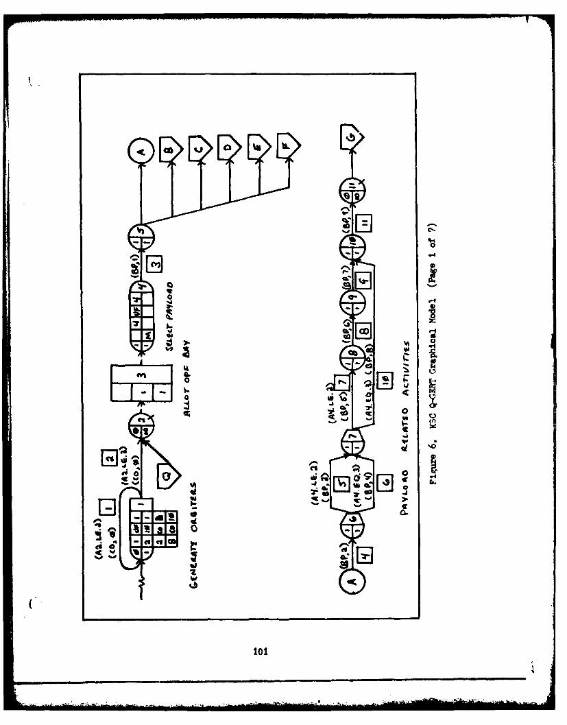
co aJ %a

rn4

EZJ

%a 0

0. ~*0.

eg o

4 lot

'a 44

* to

1I 0

43P

0-0

102)

-Ij

CIO It

044

---

CS

C CD

103

'A'

* 0

~co

00

w 0

q-*

1044

vii

Ire.

IMIS

IvaI

00

ot

rw

CL Cq.

0 a IJ

odkA-

eDAL

L%-9w

.4L

C-.-

107

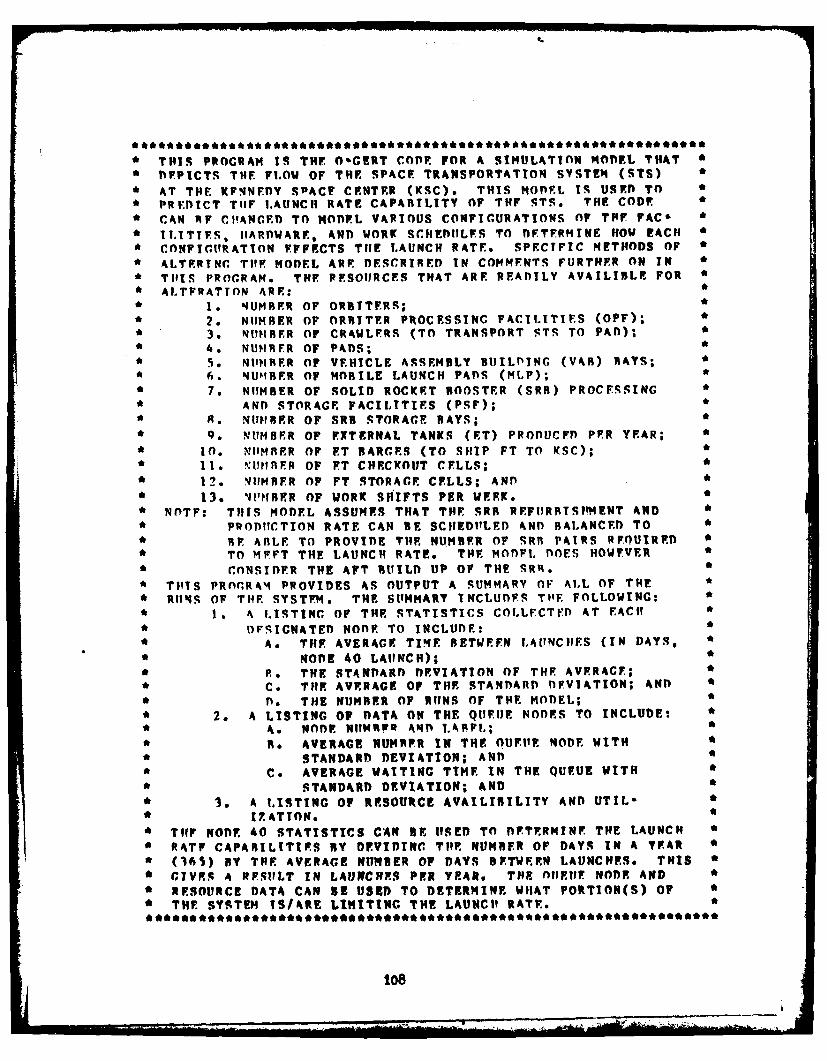
* TIS PROGRAM IS THE OGERT COPP FOR A SIMULATION MODEL THATa DEPICTS THE F1.OW OF THE SPACE TRANSPORTATION SYSTEM (SIS)

• AT THE KFNNFDY SPACF CENTER (KSC). THIS MOBEL IS USED TO• PREDICT TilT 1.AUNCH RATE CAPABILITY OF THF STS. THE CODE• CAN RF C!ANCI) TO MODEL VARIOUS CONFIGURATIONS OF THE PACO •• I.ITTFS, I1ARDWARE, AND WORK SCHEDULES TO DETERMINE HOW EACH •a CONFIURATION EFFECTS THE LAUNCH RATE. SPECIFIC METHODS OF •• ALTERINC TIlE MODEL ARE DFSCRIRED IN COMMENTS FURTHER ON IN a* TillS PROGRAM. THE RESOURCES THAT ARE READILY AVAILIBLE FOR *a ALTFRATTON ARE: aa1. 4UMBER OF ORBITERS; •• 2. NUMBER OF ORRITER PROCESSINC FACILITIES (OPF); "a 3, NUMBER OF CRAWLERS (TO TRANSPORT STS TO PAD); a

4 6. NUMRER OF PADS;5 9. NUNfRER OF VEHICLE ASSEMBLY BUILDING (VAR) RAYS; a

a 6. NUMBER OF MOBILE LAUNCH PADS (MLP); aa 7. NUMBER OF SOLID ROCKET ROOSTER (SRB) PROCESSING aa AND STORAGE FACILITIES (PSF); aa R. NUMRER OF SRR STORAGE RAYS;

q. NUMBER OF EXTERNAL TANKS (ET) PRODUCED PER YEAR;

I n, %1'1IMR9R OF ET BARGES (TO SHIP FT TO KSC);Ile P1nFR OF FT CHECKOUT CELLS;I N IMBER OF FT STORAGE CELLS; AND

a 13. 41I'?IIER OF WORK SlIFTS PER WEE.K aa NOTE: THIS MODEL ASSUMES THAT THE SRR REFURRTSIMENT AND aa PRODITCTION RATE CAN BE SCHEDULED AND BALANCED TO a

• RE ARLE TO PROVIDE THE NUMBER OF SRR PAIRS REOUIRED aa TO 1 FFT THE LAUNCH RATE. THE MODl, DOES HOWEVER aa C.ONSIDER THE AFT BUILD UP OF THE SR . a* TIS PROr.RAM PROVIDES AS OUTPUT A SUMMARY OF ALL OF THE

RUNS OF T1E4 SYSTEM. THE SUMMARY INCLUDnS TtE. FOLLOWING: aa *1 A I.ISTINC OF THE STATISTICS COLLECTED AT TACIT aa DESIGNATED NODE TO INCLUDE: a

A. THE AVERAGE TIE BETWEEN LAUNCHIES (IN DAYS, aa NODE 40 LAUNCH); aa R. THE STANDARD DEVIATION OF THE AVERAGE; aa C. THE AVERAGE OF THE STANDARD DEVIATION; AND aa n. THE NUMBER OF RUNS OF THE MODEL; aa 2. A LISTING OF DATA ON THE QUEUR NODES TO INCLUDE: a• A. NODE NlUMRIw AD I.APP,; aSRe AVERAGE NUMBER IN THE OUFIFR NODE WITH a" STANDARD DEVIATION; ANDa C. AVERAGE WAITING TIME IN THE QUEUE WITH •a ,STANDARD DEVIATION; AND aa 3. A L.ISTING OF RESOURCE AVAILIRILITY AND UTILa a• IZATTON. a• TIlF NODE 40 STATISTICS CAN BE USED TO DETERMINE THE LAUNCH aa RATF CAPARILITIES BY DEVIDING TOlE NUMBER OF DAYS IN A YEAR aa (36S) BY THE AVERAGE NUMBER OF DAYS BETWEEN LAUNCHES. THIS aa CIVF.q A RESIFLT IN LAUNCRES PER YEAR. THE oTIEUE NODE AND aa RESOURCE DATA CAN BE l1SED TO DETERMINE WHAT PORTION(S) OF aa THE SYSTEM IS/ARE LIMITING THE LAUNCH RATE. aa aaaaaaaaaaaaaaaaaaaaaaaaaa*** aa*aaaa*aaa** aa1*0***a*aaaa

108

F114CTION tlF (IF"I)

*TI'Iq IS A ]AITNCTION PROVIi) FOR By O'-.ET TPAT ALLOWq. T11F1 ISF11 TO IIAKI* 'IODIETCATYON'S. TO TRANSACTIONS A~nf ACTIVrITIEq.

*FilINCTIOJ vr IS CALLED AT NODES SPEC1 FT D 11-Y T11F PROCRAMEM*WI T11 T11F A"CUtI'* ENT I EN TIJF V'ALtF OF T EN DrTFP?,llNFS Wl'IC I' nr**TOlE VARror'C JP-TIEN BLOCKS IS TO RF 1rXFCIIT1rI. VALUEFS**Al

1'r P17TURINI' IN 11E. TIIF On'AR rnmmom P.L~ocy Is HEOUIRFn Byn 0-CEPT. rnl? A T)ETATLED ) DECRTIATION OF TUlE VARTI'LER IN TIS *

*CO',";Ot. SFF "tnODIjTTNG AND ANALYSIS H1STNC 0-rGERT NETWORKS," *

F Y A. AL.AN1 H. PRITSKER, PAGES 243-249. T11F lJCfl'1 COmnON* HI.OCK VA'[I M.LES ARE:

1.I TTAtEK-TIIE TIME AFTER 1411IJ THlE NEXT FXTERNAL TANY* MU1ST BE SENT TO VAFB,

* 2. TLANI)-THEF. TIME AFTER WHICH THEF NEXT ORBTTR 4lUST f

* LAND AT VAPH, AND* 3. TIN1Qi2-Tl1F G'REATEST END TIME FOR SR%~ qTACKINC. *

*TI'FfF VAIPT'l.FS WILL BE FURTHER DESCRIBEDI WHENM T11EY ARF USED.)

COIIoN /flVAR/ NID,NFTB(no),NRF(10O),.' 1rlp(1O),I %iRri'?(loo),NRIIN ,NRIINS,NTC(IOO) ,PARAM(ino,4) ,TRFr,TNOWCOMMOMN /11COM / TTANK ,TL.AND,TFNI12

*('11 yq TwHE ('i1.MTL.ATTVF PROBHABILTTY OF THEF VAHIOUS TYPES OF *

*PAYI.OAPSASCAE WITH TH. N11MRERS IN V'AL. TU1E DIFFFRENT**TYPES OF rAYI.nADS AND THIEIR IND)TVIDII1. ANT) CIILMITLATTVE

rpO;1AI41.1TTFS ARE:

* AYLOnAD NO TYPE pROB rill, PROHI SPACEIAB .172 .172 f

Vt1OR IZONAL .345 .,17

3VRRTYCLF .4 83 1 , (inn

SA UOR170M~A1. PAYLOAD) IS ONE TIIAT IS LOADE ~ N T11E API:.SA V'FRTICLF PAYLOAD IS ONE TTHAT IS LOAnED AT THE 1,AIINCII PAP'.tTf1F.SF TWO0 VARIABLES (CF AND) VAL) ARE IISED) To DETERMINE*T1fF NFYT PAYLOAD THIAT THE ORBITER WILl, CAPRY. f

RE4l. 4711(), VAL(3)DATA CP/.177, .517 ,1.0/, VALII.0,2.O1,1.O/

109

* TillS Prl(b' Ts CALLED) AT NODE ONE AND IT RFTURPNS To ATTRTI* 11ITF ONE THUll N'I'BFP OF 'ITSSTOKS THIAT EACto ORBITER HAS AT THE *

STApT OF TUlF SIMULATION RUY. GATRR(2) GFTS Trip VALE of **ATT'RIBUTE TWO 4PTII IS THE ORBITFR NTI9RFR ANT) UqES THIS*VAI.IlF TO DETERMINE Tiff NUMBER OF PREVIOUS MISSIONS FOR TH4E* O1#'TFP. AS AN EXAMPLE, IF ATTRIBUTE TWO EnUALS ONE (THE

*FIRST ORTITF.R) THEN ATTRTIUTE ONE (NUM1BER Or MISSIONS) IS*SET TO 71. THIIS IS DONE AT TPlE BECINNI7fl. OF THE EACH RUN. *

IF (TEN. EQ.1) THENIF (GATR(2).EQ.I.O) THIEN

lIE - 21.0ELSF IF (GATRB(2).EO.2.O) THEN

UpE - 18.0

IE - 9.0

EhD IF

*TIS liLOCV IS CALLED) AT NODF 45 AND) IS USED TO TfOVE THE*SVALV!E OF THE LAST ORBITER PAYLOAD (UIP PAYLOAD) IN ATTRI'* MTE 4 TO ATTRIBUTF 3 WHfICH IS THE DOWN PAYLOAD,

TF (lIFN.EQ.3) TlEN

UPF a GATRB(4)END' IF

*TIlTS !RI.0CV IS CALLED FROM NODEF 4 ANT) IS USED TO DE.TERMINE

*TIlE NEXT PAYLOAD (UP PAYLOADb) FOR TilE ORBITER. THEF PAY'-*LOAD IS RFI.FCTF.D UISINC THE TDPROB FUNCTION A~II) THE VARIABLES*SCP AND VAL.. THE ARGUMENTS FOR THE FUNCTION ARF. CP (THE.*CULMHITLATYVF PROBABILITY FOR EACH CHIOICE), VAT. (TIE VALUE

or OFACII POSSIBLEF CHOICE), THE NUIMBER OF POSSIBILE CHOI1CES,aANT' TItF NUIMBER OF THE PARN~l NUflRER STRTNC TAn~ tFITSrn.*TIlF RANDOM NI'IRER STRING IS TNTRTNSTC TO 0-GERT. nPROR *

* USrs A !OnKTE (rARLO SELECTION TP.CHNTOUF TO SELETCT TIIE PROB-*ABILITY ANT) THUlS THE VALUE OF THE CHIOICE. npROB RETURNS *

*ONE OF THEF I POSSIBLE VALUES IN VALUE TO 11F'. THIIS VALUEISj TIIFN PLACE!' IN ATTRIBUTE 4 (UP PAYLOAD),.

IF (IPN.EO.4) THENlUE - PPROR(CP,VAL,3,2)

FND IF

110

*THIS TrlOfCK IS CALLED FROM nDE 13 ANn DF.TERMIKF.S THE TYPE**OF qSlqEI PERIODIC qlIGNIFICANT SPECIAL TASY THAT MUST RF*PERFOP'IFn (IF ANY). THEF TYPE OF PSST TPAT 15 DONE nF-*PFNns ON T11F NUMBER O MISSIONS TIIAT TH1E ORBITER H1AS BEEN*ON. THEF NUMBFR OF MISSIONS OF THEF ORBITFR 1S MAINTAINED *

* I ATTRTHIITI* I AND) IS RETRIEVED USINC TFF CATRB FlTNCTION.*TIIlS VhIl'FR IS THEN COMPiARED AGAIST THEF PSST REOUIRF.MENTS*TO PFTFTPI!NF '4HICI' TASKS ARE PEOI'IRFD. IF TWO PSSTS ARE* OIT-'~ TlfE ONE WITH THF LOnNGEST RFOIJIR ED TIME IS DONE.*T11E PSSTS ANDn THF FLIGHTS ON 'JHICH THEFY ARE ROUT1RED ARE:

1. *II CUr~ PIR SShJRF FUEL TIIRRO PUMP INSPECT: EVERY 2 FLIGH1TS* 2. 'IYCI' PpEssIIRE nXIDI7.ER TUIRBO PlUMP: EVERY 5 FLIGHTS* 3. EK(114F REMOVAL AN'D REINSTALLATION: EVERY 9 FLITGHTS*

*AS AN E)XAmP1E IF THE NUMBER OF MISSIONS IS A MULTIPLE OFI TIIFN IE IS SFT EQUAL TO 1 AND THIS IN TURN SETS ATTRIBIJTF

5 TO 1. T1E. TRANSACTION THEN BRANCHES ON A/TRIBUTF 5 ANn*SCIFDI'LFS T1lE TASK REQIJIRFI) FACt! TWO FLIGHTS.

IF (IFN.EQ.5) THENATI, - GATRR(1)IF (AT1.EQ.0.0) THEN

11F - 4.0ELSE IF (AmOD(ATI,2.O).F.l.) TIIP.N

UF - 1.0ELSE IF (AMOD)(ATl,5.O).EO.O.0) THEFN

UF - 2.0ELSE IF (AMOlD(ATl,9.O).FO.O.O) THEFN

VF - 1.0FLS F

UF - 4.0END) IF

END IF

STPlTS BLOCK IS CALLED FROM NOD)E 19 AND nETERMINES THE TYPE*OF ORRITFR PSST THAT MUST HE PREFORMED (IF ANY). THEaSMFTHOD OF SELEFCTION IS THE SAME AS IN THE ABOVE BLOCK,*TH1E PSSTS AND THE FLICHTS ON WHICH THEY ARE REOHIRED ARE:

a 1. PAYLOAD BAY THERMAL CTL SYq REPL.ACEMENT: EVERY 40 FLTS* 2. PARTIAL PLB THERMAL CTI. SYS REPL.ACEMENT: EVERY 33 FLTSaa 3* FUEL CFLL. REMOVAL AND REPLACEMENT: EVERY 12 FLTS a* 4. API REPL.ACEMENT: EVERY 13 FLTS

IF ( IFN. F?. 6) THENATt - (;ATRR(1)IF (ATI.ro.n.0) THEN

rIP S.0P1 IF (AMnyD(ATI,40.0).EO.O.0) ThIIN

1 .0

I E F (AMOD(AT1,13.O).F0.0.0) THFN'Ill - 2.0VI.SFE TF (AMOI(ATI,I2.O).FQ.O.O) TIFI

IlF - 3.0ELSE IF (AlnO(AT1,13.n).EA.0.O) THEF

UF - 4.0ELSEF

(IF - 5.0

FNI) TV

*TIlT S 11,nCv 1S CALLED AT NODE 44 AND IS IISFT TO ;FI.FCT THE.*I.ANnTN"r SITE FOR Till' OZB ITFrr. TIF ('!*RRiNT 1SitIUL1ATION TIME*IS COMPANRfl TO THE TTMF CONTAINED 1IN TLAND (TUEF TIME AFTER*WI111171 Till- MPI'T OR1RTTFR MI!ST 1RF SENT To VAFP). IF TIZOW is* CPFATI TI'FN TLANYD TI'FN A T'") IS PLkrr TPTRIIITF SEVFN *

*AfkI TI'': n,1r'rFP 15; sNT TO V'APII TLANI) ' TUil-N 1'PDATFn TO *

* III.FC'." Till* TT1F AT WI1TCH4 TI1F NEXT WTER 143 SENT TO VAFI1.It: T'"flI P; 'InT CRF.ATFR TItEN TI.AND TTHEN A ONE IS PLA'CFn INTO

* 4?TQTR1!Tl'rF PI ANY) TUEF ORPITFR IS SPINT TO VtSC. TIfE VALUE

* AIflFb TO TI.A"ml' (16.5) IS -qf.FCTFfl SO AS TO -SENT TFN ORBTTRS*T(I VI'AF '\ VFARl. TIlE OR'W TFEr% ARE' SENT TO T 1 F CHOSEN 1.Arn.*ING '1 TP IY IRRANCHING FROM NODE 44 ON TI'E VALIuE IN ATTRtIUITI'

I(IP' .Fo.7) T"ENIF (TNOI4.GT.TLA~n) THFN

111' 2.0TLANIP - TLANDh + 16.5

-' I *O

1 12

* Tills RI.OCv IS CALLED FROM NODE 8O AND IS USE) TO SFI.FCT TII ** D iSTINATioZ FOR TIll PXTFRNAL TANK AFTER tP, on1ICTION. TIE *

* 4I.O('v 1Is T!"E SAME .OCIC AS TIIAT D.SCRItF F OP TilF SIFC- *

* T!Ow OF TIliF I.A InlNC SITE FOP Tiie ORBITFP !FNTIONE, AROVr. *

* TillS 11l.0(7' ALSO FENDS TF.. EXTFR,AL, TANKS A VFAR TO VAFP. *

IF (IFN.F*o.R) TIIFN11- (rNot'.CT.TT NIK) TFi''

IF - 2.0TAx- TTANK + 16.5~

FI L F

i' l l. I .E "NI) I I

F111) T

* Tills PI.Ort IS CAI,LFrn PRIOR TO SRIt STACKING IT TIlE VAR. TITS ** IS DONF T' DELAY OTHER ACTIVITIES IN TfIF VAR DUE TO SAFETY *

* TIP1F',S THE IFNCTII OF TPF SRR STACKING PROCESS (TIME) *

* IS l)FTF1i['FI0 FTRST USING PARAMETER SET 26. TIlE END TIME *

* FOR TilF ;rA,\(;KINC IS rDETERMINED BY ADDINC THE STACK TIME TO *

* TIF Cl!RREN T SIMULATION TIME (TNOW). TIlE END TIME FOR THIS *

* STACK (TENDI) IS COMPARED TO THE LAST SRB STACK END TIME *

* (TFNn2). IF TENi IS LESS THEN TEN!)2 THEN THE OTHER ACTIV *

* ITIPS APF ALREADY DELAYED PASSED TIlE STACY TIME AND TIIERE

* IS NO NEF'n TO EXTEND THEM ANY MORE. IF TEF:)I IS GREATER *

* TIAN TFnT)2 THEN TilE VAR ACTIVITIES MIuqT BE DELAYED. IF *

* TIERE AIRF NO CIIRRENT SRR STACKINGS OCCIIRRTNC TIIEN THE ACT,

ARE DELAYFn FOR THE FULL TIME OF TIlF CURRENT STACK (TIME). *

* IF Tl'FRF IS ANOTHER SRR STACK IN PROCESS TIIEN THF ACTIVITIES *

* ARE FXTEJIFf BY THE DIFFERNCE BETWFEN THE CURRENT STACK *

* TIME AND THF NEW STACK TIME. TIlE ACTIVITIES ARE DELAYED BY *

* ItIINC Till XTFND SURROPTINE. THIS SUBROUTINE IS INTRINSIC *

* TO 0-,CERT AND HAS TWO ARGUMENTS. THE FIRST ARCIMENT IS TIE *FSA;TTVTTY f'7!?IRFR OF THE ACTIVITY TO HE DELAYED AND TT!E SECOND *

* AR;II"MN T IS TIl- LENGTHl OF TIME THAT THE ACTIVITY IS TO RF ** fiI.AYED. IF THE ACTIVITY TO BE DEIAYED IS NOT CtTRRENTIY IN *

* PROGRTSq THEN THE RFQUEST IS IGNORED. FINALLY, THE PROCESS ** TT.E FOP Till' SRI, STACK IS PLACED IS ATTRIRITF SIX AN! THE a* ACTTVTTV lS BFGIIN.

113.

TV (I P'.. FI.) T PENTT- IBF(26)

TFNDI TP F + TNOWIF' ( TFNflI * T. TFND2 ) T)10!~

It' (Tt'014.rT.TFND2) TI1rNTIIIFI -TIMF

TI"Fl - TENDI *TF14r2

C AI, I TFNfl (62 ,T14FL)C A 1. 1 vT F;n (65,TTMFI)

C A.1. TPNO (6q JIMYIF1)C A1. 1. XTENI) (7O,TIYI)C A .1 XT F m r (77 ,TIMFI )TF ' -112 - TFNIll

r- 'n I r11 TIME

F'~rP IF

*T"Iq PI1.flv IS CALLFT) PRIOR TO MATING THF. OKBITFP TO TTIF, sRR/*FT ASR rM~tY Y. FIRST TPRF PROCESS TIME. FOR TIlE MATINr 1S flF-

*TFRMrNFI) (TIMF2) USING PARAMETER RFT 10. IF TlIFRF IS A SRB

* -rACV CII'RPFNTLY IN PROCRFSS THFN TIlE pI~0CFqS T1'llF IS FXTFND)E)*

* 'Y TIIF Altol'NT OF TIME LEFFT TO COMPLF:TF TI-IF SRB STACY. TIlTSI S (rmft~ FflP SAFETY REASONS THAT nn NOT? AI.O)!4 ANY flTI'FR V'AR

*ACTIVTIS JIIFN TIIFRE IS AN SRR STACK nCCIIR [NC IN TIFF VAR.*IF TI'FRF I', %'!T A SRR STACY IN PROCRESS TIIVk TIFF ORGTNAI.*TIF Fol' TIlE OPIIITgR MATE IS ITSFn AS TIFF ACTIVITY TIMF.

IF (TEN. F(1.I) THEFN

TI7MF2 - TIF(20)IF (TI.ND2.C.T.TNOW) THEN

TP!IF2 - TIMP2 + (TEND2 - TNOII)

I'F - TIIPE2

*TRIS RLOCK IS CAILLED) PRIOR TO MI.P RFHRRIHMENT IN TIFF VAR.*TIFF PROCriSS TIME IS THEN EXTENRD IN THlE MANNFR DFSCRIRFI)*PRIVIOI'SLV IF A SRR STACK IS TN PROGRESS. A CONSTANT TTMF

SIS IISFI U'OR THlE ORIGINAL MLP RFPIlRRTSIfMFNT TIMF.

IF (Tr-4.J.F.11) THENIF (TI N)2.GT.TNnw) THEFN

IIF 1.41 + (TFIJI2 - TNqOW)

tiI' - 3.43FND IF

P.NI IF

114

" TITS RLOC'( IFlTFRMINF. TliE PROCESS TIME FOR TlE. SRtB CPECKOUT" fPFRATTONS ISINC PARAMFTFP SET 27. IF TIIERF IS A SRIK STACW" (WRPENTI.Y IN PROGRESS TPFN TfIE ACTIVITY TTME IS EXTENDEI) AS*PRFVlnttSI.Y OF.SCtTR~fl.

II, (Tr!!.FOn.12) THFNTTIFI - BF(27)IF (T~mn2.GT.TNOW) TJIKNTIMF1 - TT'3 +- (TFNn2 *TNOw)

FMP IF

J-.NJ IF

*TVIS vkj.Oc.v CALCULTATES TI?? rT MATE PRnCFSS, TTME I'SINr PARA- **'IFTER svT 2P. TIIE TIME IS EXTFNDET) AS AROVF WIIFN RFOnUIRpD.

TF (TFN.Fo.13) THFF

TTMF4 - RF(?R)IF (TPP12,GT.TNO4) THEFN

TTiF,4 - T111F4 + (TEND)2 *TNOW)

11F - TIMF4FM!) IF

*T'IS BLOC'( CALCULATES THlE E.T/SRB1 CllFCVOlHT OPFHATIONS TIMF* i'Jr~ PARAIFY:TER SE7 29. TNE TIME IS EXTENrDED AS RPnhiTRFD IN*TI'E SAMIE M'ANFR AS ABOVE.

IF (TFN.i.l~4) THEN

IF (TF~fl2.CTTNOW) THEFNT14FS - TIMES +- (TEnD2 TROW1)

1- TIMF5UlDr IF

TI1TScW ()CAlCIATFS TIIF FT CIHECVOIIT ()PVPOTTnOc% TTMF USINGC*P'APA'1ITFI! qSF;T 30. TUEr TTME I-, FXTPrtBP AS AIROVE WlIFN NEFI)Ffl

IF (IF*.E.O.15) TIFN

TT'-irf, - RIF(1O)IiP (TFIP2.CT.TNOi) TIFN

TOC- TINIF6 + (TFNn2 -THOW)

IIF T 111F6F%4I) IF'

V F TI' P"

*TIIS SIIMUOITINEF IS CALLET) AUTTOMATICALLY BTY TjUF n*CF.RT ANAL'*YS-'IS PROCHAM AT TIlE. BEGINNING OF FACTI RUN OF TIlE. NETWORK.

*TIITS SIf~fI!ITTNF TS UTSE9f TO INITIALI7.F THfF VALVES.! OF TTANY,*TVANI), A-411 TF.NT2. IN ADI!TION, ON THE. FIRST RIIN * TPE PARA-

* r1TFR SFTS IT'SFn IN THE IUSER FIINCTION ABOVE (20, 26, 27, 2R,*

*2'?, A~n 10) ARE. TNTTALI7.EP. CPRP IS AN INTRINSIC ROUITNE

*IN n-CrFT TIIAT IS USED TO INTIALIP! PARAMETER SETS TO BE* lTIIT"VFn AS A PFTAk-PERT n7'STRTRITION.

I NRITPI.(100),NRIJN,NRI!NS,,NTC(Ino) ,PARA'l(Inn,4) ,TBFC,TNOWCOm1MON /vIm/ TTANK, TLANfl, TFNT)2TTA41V - 36.50)

ThAN!) - 16.50Tn?- 0.0

IF (MRIIN.f7O.1) THENcAit . . rIIP(2n)C A 1 1 CIhlP(26)C 4 ,l1 rPhIP(27)C Al. 1, CP It1( 2R )CALL CrIRP(29)C A 1.. CPRP(30)

FN!) IFR M.I'R NFNn

116

*THEF VOIl.OVTINC PORTION OF TVIE PROG~RAM IS TilE O-C.FRT COMPITFR*

RFPltFSENTATION OF THE NETWORK DESIGNED TO PEPICT THE STS

*FLOW AT VSC. THP PROG~RAM UTTL7,FD T1E. flCFRT ANALYSIS PRO-*CRAM TO ANALYSE THE SYSTEM. FOR A FULL nFSCRIRTION OF THE*PROGRAM4 STATEMENTS AND TRETE. PARAMFTFERqS FF "MOnFLINC AND

*ANALYSI, IISING n-CERT NETWORKS", RY A. AL.AN R. PRITSKER.*TVHE PROCRN % CCO'IPLISHFS 10 RL'flS OF TIIE kiODEL WITH* ACII !,,Ut! !IFTNIC 4015 DAYS IM' 1,FPJCIIT Twir FIRST 365 DAYS ARE*ICN()RFP POP STATISTICAL rCIICLATIONq. TilE OUITPtT IS A StlM-

* 'ARy nF ALI. TER OF T1lE PlINS.

FANDRUISVS VN, KSCOPS ,10, 30, 19R2,12, .. 4015, 10, , 365 .R*SOIl, I, ,A SOUlRCE FO0R ORBITERS

hrT,l,1,CO0,I,()A2.LF..2* GEN'RATFS ORBITERSArT,I,2,Ct),O.0,2,(4)A2.LF.l* SENDS ORBITER,; TO WAIT FOR

* OPFOh#,2/'ATl'r,(Ir)yl* ORBITERS V*AIT FOR ~fF RAY

PSTABLI1SP'F. T11F NUIMBR OiF* OPP RAYS (2). TO Ann ORa DCI.FTF RAYS PUT THIE lF-a SIRED ffiMRFP TF PLACE* OF THE 2

A I..13 ,i2 /4~ ALLOTS OPF RAYPEC,, 1 I~n?4*ORBITER ENTERS THF OPE ANDa IS MIARKED) WITH THE CURRENTa TIME

VAS R,4,4,tyr,/4* SELErCTS UP PAYLOAD%

ACT,4,5,EP,1,3/SFORR* ORBITER IS SAFpn PRIOR ToSERVICI NC

H EC ,5, i, 1'

ACT,5 ,6,R,2 ,4/PLBACCES* PLR ACCESS IS GAINED

SE.,6 ,1, 1 ,*ACT.6.7,BP,3,5/REIIORPL,(9)A4.LE.2* REMOVP HfORIZONTAL PAYLOAD

ACT,6,?,BP,4.6/RVFRPT.,(9)A4.EO.3* REMOVE VFRTICLF PAYLOAD

AC.T,7,R9upl,5,7/iiO)RFLKT,(Q)A4.1LE.2* INSTALL H1OR. FL.IGHIT KIT

ACI,R,'),1 P, 6 8/lNl4ORPL* INSTALL HOPR. PAYLOAD

ACT,9,1O),Pp,7,9IORPLCXOtIT* l'OR. PAYLOAD CiIF.CKnIfTAGT,7,10,RtP,f1,10/VF.RFLTKT,(9)A4.P.O.3* INSTALT. VFP. FLIGHT KIT

ACT,1O,11,1RI',Qi,1/FINLTCfl* FINAL PLR CIIFCKOITTfluF,II/VArI'ATNT,(IO)25* IYAITS FOR OPE MAINT. ACT-

TVIIFSTO RECOMPLETED

L7V.I.S R

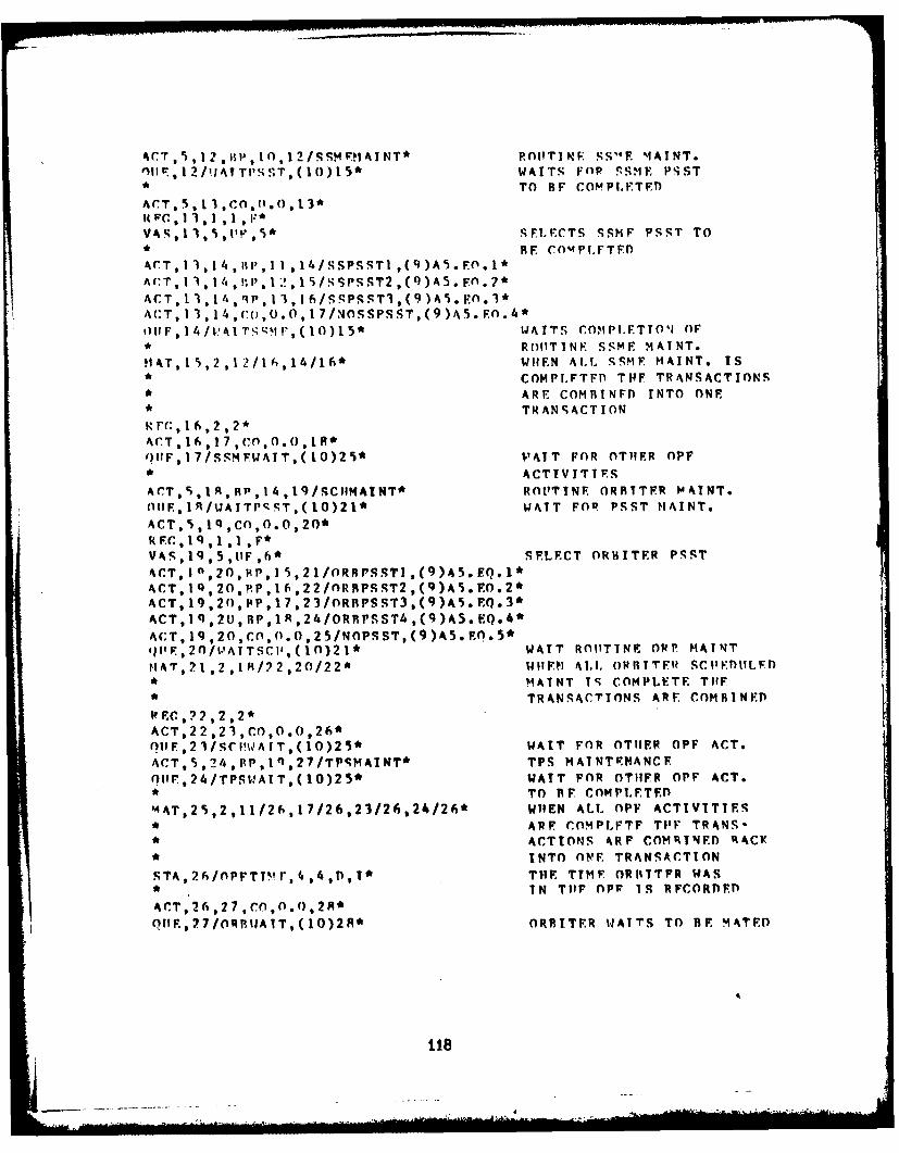
ACT , 5 1 , I,OI2/qSSMEMIA INT* ROUlTINEF !S"EI MAINT.

* TO BF COMPI.ETF)

ACT, 5, 1 1.*CO.0.0,13*

VAc',#11 ,5,I' ,* SFLF.CTS SSMF PSST TO* RBE COM4PIFTFI)

ACrT,13 ,14,iH',,1 1,14/SSPSSTI ,(4)A5.FO.1*ACT, 11,I4,1,P, 1:!,15/SSPSSqcT2,(9)AS.FO.2*ACT, 11 ,11, 11P, 11,I16/SSPSSTl,(9)A5. F.*

AACT, I 1,14 , C o, 0. 0, 17 / NnS SPS 1;T, (9 )A5. Fo * 4*Mf F , 1I !A I T5'%11, ( 10) 15* WAITS COMPLEFTTO4I OF

* ROIUTINF. SSMF MAT NT.H1AT. I5,2,12/16,t4/16* WHEFN ALL. SSMF MAINT. IS

* COmptFTED THE TRANSACTIONS* ARE COMBINFD INTO ONE

* TRANSACTION

ACT,16 ,17,COn,0.0,tP*()lTF,17/SrMFWATT,(I0)25* l'AIT FOR OTHIER OPF

* ACTIVITIESArT,5,,RlP, 14 ,19/SCHfMAINT* ROVTINE ORBITER MAINT.OIlFI91/WArTr4cST,(1o)21* WATT FOR PSST MAINT.ACT,5 ,1Q,CO,0.0,20*RFC, 19,1,I,F*VA\S, 19.5,IIF ,6* SELECT ORBITER PSST'CT,I1 ,20, lP, 15,21/ORRPSSTI,(9)A5.EQ.1*ACT,19,20,RP,16,22/ORBPSST2,(9)AS.EO.2*ACT,19,20,14P,17,23/ORBPSST3,(9)AS.Eq.3*ACT,19, 20, RP,1R ,24/ORRPSST4 ,(9 )A5. EQ.4*AC'T 19,2O, CO , .0,25/NOPSST,(9)Ak5.EO.5*qII,2O/IJAITSCl',(I0)21* WATT ROUITINE OPP MATNTtMAT,2,2,1Ri/22,20/22* W11FM ALL ORBITER~ SClIIFY)F

* MATNT TS COMPLETE TflF* TRANSACTIONS ARE COMBINFD

PE.C,?2 ,2 ,2*ACT,22,23, CO ,0.0,26*O)llF,21/qCflWATT,(IO)25* WAIT FOR OTlhER OPF ACT.ACT,5S,!4,PP,1fq,27/TP9MATNT* TPS MAINTF?1ANCFntir,24/TPSWlAIT,( 10)25* WATT FOR OTlIFR OPF ACT.

* TO BE COMPLETEDM~AT,252,1/26,17/26,23/26,2 4 /26* WIIEN ALT, OPF ACTIVITIES

* ARE COMPLFTF TI'F TRANS-* ACTIONS ARE COMBIRI) RACY* INTO ONE TRANSACTION

STA ,26/0PFTTmlr, f.,4,1 ,T* THlE TIME ORITTER WAS* IN TilE npr IS RECORY)ED

ArT ,26 27,cn,O.o,2M*ql?F,27/ORRUlA1T,(10)2R* ORBTER WAITS TO BE MATED

118

S F., 2R/0RRMATI,ASH ,iRs, 27 784* VIkIF.N ROTH! AN ORBITER* ANt) A qRK/FT AS%0R.Y* ARE AVALYBLE. TIlE OFRRTFR* MATING ACTTI"TTY Iq RFCLIN

ACT,?R,2Q ,CO ,0O.29*FRF,2q, ,I ,.3* TIlE nPF RAY 1S FRFFn!

* FOR TIIr XF'(T ORIITF.RACT,2q , 3fl~c,nlO),1/TOWTnVAR* TOw ORIITTFR TO VARRFr,lo,1 ,I*VAS,lO,6,IiF ,lO* PP.TFRMINF ORB MATE TIMEACT,3O,32,AT,h,32/MATEORB* MATF ORBTER TO ASSFMRLYnhF,12/WATCRAI',(10)33* ASSFMALY WAITS FOR CRAWIFRRFS,2/CRAWvLFR,l3* FSTARLIS11PS NIIMfPFR OF

* CRAWLERS (1), TO API) CR'kW*T. FR PITT Tor DF.sIR Fl NUN'

* RER IN PLACE OF THVE IAL~L,,33 ,,2,I ,32/14* ALLOTS CRAWLFERnl'F,34/IATPAn,(10)35* ASSEMBLY WAITS FOR PAD)

PFS ,3/PA),2 ,35* ESTABISIIFS THE NIIMRFR OF* PADS (2). IF IT IS DE.SIRED1* TO Ann) OR SUBTRACT PADlS* CIIANCF THE 2 TO T14F* DESIRE!) NIIMBR

Al.!., 15, ,3,I ,14/16* ALLOTS PADR PC ,16 ,1I,1I*

ACT,16 ,9A,cn,o.n,A4*FRF,qgR,,f6 ,I fh* FEI" VARACT,A, '14,( 0,0.0,I5STA,9q/RFTvA,,1,n,o*ACT.36,17.cn,o.fI,33/TI.ITOPAn* riOVF hSSFMRI.Y TO PAD)PFC' 17,11

ACT, 37,18, o,.h1,34/RTCRAWI.FR* RFTIIRN THE (CRAIIlERFRF,3 ,2,,31*FREE CRAWLER FOR* FURTHER USF.

ACT, 1R, Q, CO, 0.0,35*STA,1Q/RFTrAT., 1,1, I)

ArT,17,40,RP,21,136/PArDoPS* PAD OPERATIONS TO yNcI,IIDP* TII CnIuNTD)OWN

v*TA,4fl11.AUII,1 ,,R* .AUNCII Tiw nR1IITE.R AND* RECORD) TUEF TI'4F BETWEEN*C0ONSFECITIVF ,ILUNCHES

VAS,6O,1+,Co,1* UPDATE MISSION COUNTArT,40,4j,CO,6.R1,37/RFRRPAl* RFFUIRRBII LA1.1Ch! PAD)

FPY,1 , 3,1 35*FREE LAUINCHI PAD) FOR

FURTHER IISEACT,41 ,42,rO,0.n,39*STA,I.2/RF.TPAn,1,I,lb,B*ACT,40 ,A1, co,0.O, 39*

ACT,A3,AI.,NO,22 ,'O/SLMI SS.,(9)AA. FO. 1* SPACFLAR MISSION TIMEACT,41 ,44,No,23,41/NOMNISS,(9)A4.CE. 2* NOMINAL MISSION TIME

119

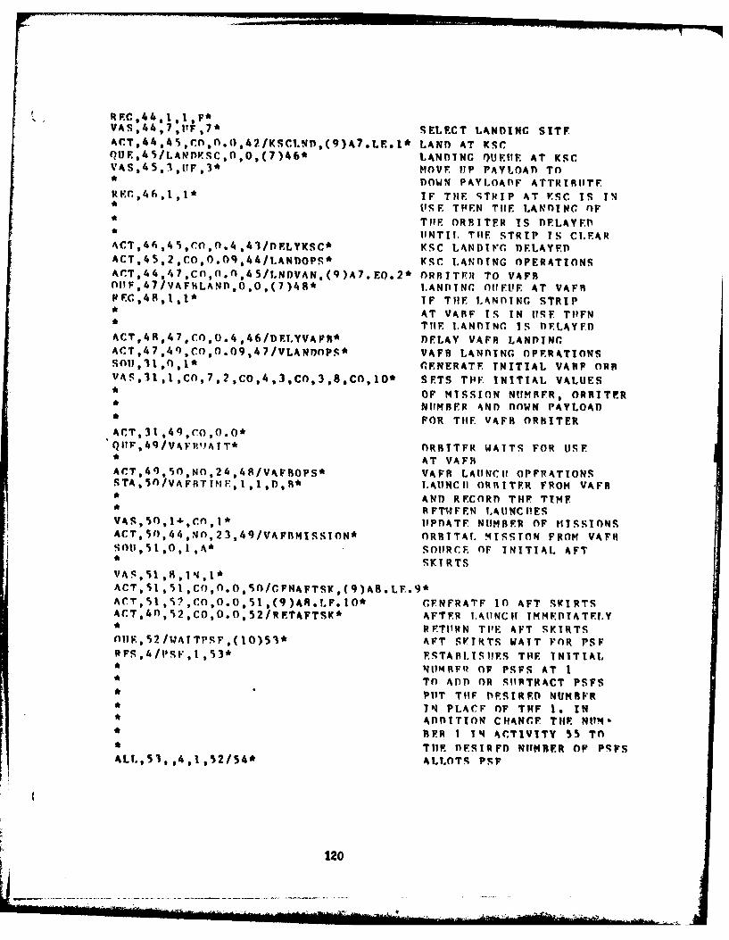
RFC.44,lI IF*VAS,44,7,11F, 7* SELECT LANDING SITEACT*,A,C ,ri0 .0,I.2IKSCI.nD,(9)A7.LE.I* LAND AT KsrQUF.,A LAKnfVC,0,O,(7)46* LANDING QUE1E AT KSCV AS ,45,3,IIF, 3* MOVE 11P PAYLOAn TO

* DOWN PAYL.OADE ATTRIR!ITERvE.,46,l ,1* IF THE STRIP AT V.SC IS IN

* IUSE TPEN THE LAnDING OF* TIlE ORBITER IS DFLAYED* UINT11, THE STRIP IS CLEAR

ACT*4fu 45 ,cO,O.4.4l/nRLYvcSC* KSC LANDIFC DELAYEDACT,45,2 ,CO,0.O9,44/1LANnopS* VSC I.ANnYNG OPERATIONSArT,44,47,CnI,O.nA5/LNDVAN, (9)A7. EQ.2* ORRITrER TO VAFR01IP,47/VAFBLANDI,O,O,(7)48* LANDING OflFUE AT VAFR

RFC,4,1,1*IF THE LANnING STRIP* AT VABF TS IN USE TtIFN* THE LANDING IS DELAYED

ACT,4R ,A?.cO,O.4,46/DEL.YVApR* DELAY VAPB LANDINCACT,47,49, CO,.O.9,47/VLANnnPS* VAEB LANDING OPERATIONS

5011,1 ,Ol* GNERATF INITIAL VARP ORR"AS,31,1,co,7,2,co,4,3,Cn,3,8,CO,1O' SETS TPF INITIAL VALUES

* OF MISSION NIUMBFR, ORBITER* NUIMRFR AND nOWN PAYLOAD* FOR THE VAFR ORBITER

ACT, 31 ,49,cO,O.0*QllF,4q/VAlVI!IATT* ORBTTR WATTS FOR USE

* AT VAFHACT ,4qSO,NO,24,48/VAFBOPS* VAFR LAUINCH OPFRATIONS

STA,0VAB~fM--,~lDR* AUNCHI ORBITER FROM VAFR* ANT) RECORD THE TIME* BET14EEN LAUNCHESVAS,50 1+,C,1*UPDATE NUMBER OF MISSIONS

ACT,50),44,Nn,23,49/VAFBMISSION* ORBITAL. MISSTON FROM VAFRSOUlO,,A*SOURcE OF INITIAL AFT* SqKIRTS

ACT, 51, 1, CO, 0. 0, /C ENAFTSC,(9 )AR. LE. 9*ACT,51,S?,CO,0.0,51,(9)AR..E.10* CFNFRATF 10 AFT SWIRTSACT ,40 ,52.CO,O.O,52/RETAFTSK* AFTER L.AlNCH IMMEIATTLY

* RETIIRN TPlE AFT SKIRTSOIIF,52/WATTPgE,(10)53* AFT SVTRTS WAIT FOR PSFRES,4/11SF,I,53* EqTARlITSIES THE INITIAL

* NIIV4RF OF PSES AT I* TO ADD OR SITRTRACT PSFS* PItT THlE DESIRED NUMBR* IN PLArF OF THE le IN* ADDITION CHANCE THE NlM-* %ER 1 IN ACTIVITY 55 TO* THE DESIRED NUMBER OF PqFS

ALT.,51,94,1,52/5.* ALLOTS PSV

120

Oi54 5% (rj 0.7,5/AFTTVAN* INSTALL.AF SITINSTN

nhlE,5%%/UAITSPH I(10)57* AFT grI!PTS vAIT FOR SR4Ar-tII41).-i,CO ,O * 0,%4/R ETSR'1* RFTIlRN SR4 AFTER LATIN('I)IF,6/ATAFTSK,1O,(1O)57* SRM WAIT FOR AFT SKIRT

* STARTS WIT11 10 IN nIlFIIF

ACT,57 nI,5%/i ImihP, I* AFT RUT.1111P OF SRR TN PSE* NTIMIIEP OF SERVERS 0I IN* T)I!S CASF) 11IIST E.QUAL THE

ffIPF8ruH/AT'TnTR,(10)59* STRS WAIT STORAC.F

RESS/StVsTroifl,2 * 5C)* I"TARLTI~hIFS NUMBERFR OF SRR* STOIIAC~ %AYs AhT 2. TO Anl)

* OR T)FI.FTF STORAGE PLACE* TfIF ORSIRE! NIlMRFR OF* STORACF RAYS IN PI-ACP OF

AIl. ,c.I,,5 A/6 0* ALLOT SP1R STORAGE1! F ,60, 1*A1CT ,60,6'., CO ,.0,56*FRF,61, ,4 ,1~,51* FREE PSF

ACT.6,6h1 ,Cn,f0.0, 58*nj'F,fi1/WAIT'TTP,(lO)69* SRR WAITS FOR MLP ANT) VAR

.,n11, 64, , ,1A* qOUACE COR '11.P'S

ArT,64,,% , ('), 0.O),60,(9)AS.LF.3* GEFNRATE I %11.P'r

ACT,40,6%,CO,5.43,61/WA-.hlML.P* WAS!? MI.P AFTFR LAUYNChI ANI)* MOVE TO WAIT FOR VAR

O1F,6s/wAT-rv~ii,(lo)66* MLP WAITS FOR VAR

RFS ,6/VA R ,2,66* FSTARTSIF! THEF NUMBER OF* VARS AT 2. TO ADT) OR

* LETF TlIF VARS PITT THF DF.'* STRF!) NUlMRER IN PLACE OF* THE 2

A1.L?, 6 6, ,6 1 * - If,/7~ ALLOT THE VA!'

VAS ,67 ,6 ,!IP,1I* D ETERMTNI'rL RFFIHIRISIIl* MFNT TTME

ACT,67,69,AT,6 .62/MLPRPFIIRB* RP.EURBISII MLP()IF,iP/tPAITSRl,(10)6q* 1'ATT FOR SRR SET

SFEL,69/9TACXSRR,ASM,(7)6i3,6fl* WHEN BOTH THE RRAS ANY)* THE MLP/VAN ARE AVAILIRLEft SRB STACYINC IS STARTED)

ArCT,6q,7O ,e ,O.0,631*

VAS,70,i,ijF ,9* nVTERMINF SRR STACY T~tHPACT,70,?l ,AT,h6,fiA/SRRtSTArK* STACK SR!nS ON ML!'

FREE SRR STORAGE

STA, 97/A FTSRRST, 1, 1,!),8

121

, 2e6, .

Vkq,71,6,,rF 12* DETF1RMTNF SR1I ChE9CYOUT* TINIF

ACT,71,72,AT.66/SRBALTNF* SRR CiFCfO'T AND ALIGNMIENTOhhIv,72/WATFT,(tO)73* WAIT FOR FXTFRNAL TANK

sFL,73IET 'vrF,A O,7)2(4 WllFN AN FT AND STACKFD)* SHBI APE AVAILIR.F TllEN T11F* ~FT MATING IS TFIECIN

ACT,71,74t, o ,O.O ,66*Ir74 ,1 ,1~*

VA- 974,6 ['F I -,R cn,n* nFTFRMINI'S FT PATE TIMF

ACT,74, 77,AT,h,h9/MATEVT* MATF FT TO qRH

ACT ,74,*7 9,CO,.O,67*1--'t ,7S, 1),j ,inTFR,?F rT eTORAcr

AT, ,7 ,FT ,r';T. Fl,6R* n,

ii".:, 7 7 1 1 I*VAS ,77,6 ,11: ,14* flETFPMTNF FT/SHIR CHECrKOUT

* TIMl FACT,77.79.AT,6,70/FTSRBCO* FT/SRRt CI'FrVOIITonjFv7R/WATTOl!R,(1O)2R* WATT FOR ORRTTR MATE.

,n! 7 n ,)J, 1, I,* qtOU'lt(:rFnR FXTFRJAI TANKSM~rT, 7Q1,17,rC,.21,7/PRO)7T5.* PRODI'CF FTq AT A PATE

OF~ 24 PEP YFAR. TO 1N** ~CRFASF T11F PROTICTION RATE.* CIIANCE rw1 nrYS BFTWFEN

* rroflhlTO'~ (CIITPREM'TLY

ACT, q ~i* 072*15.21) TO T11F nESIRFID RATF

VAS,~),7 ~q* DTERlIN'7 ET DESTINATInNAC'T,R'),.Il,CO,f).n,73/PTTOKSC,(q)A7.Ffl.I*VT SF"T TO KSC

(lF,l/WATTHAQ(;,(10)92* FT WATTS FOR RARCE

vF,,7/vSC'.A4CE,4 ,92* r~qTAR1.ISIIEFS THE NVMHER OF* KSC RARrrr. (4). TO An" OF* PF.LF.T RARGFS PIT THE. DF.

* SIRP.D NWIRFR TN PLACF OF* Ti4E 4AlJ P2,,,1,R/R3*ALLOT Yqr RARCF TO FT

ACT,T1.3,P4,C(,7.O,74/Sts1PTOKSC* SIqlT FT TO vsc

OIIP,4/WA!TrTC0,(1I))RS* FT W.ATTS AT KSC FOR* AN FT ClF.CY0hIT CELL.

HFS,R/FTrC,CLL ,2 ,R* fSTAPLISHEFS T11F NIIMRFR OF*FT ClircKOUT CELLS (2). TO

* Any) oR DELFTE rlF.CKOllT* CELLS PUTT T11l EITRED*N1UMBER OF rFI.I,c, IN PLACE* Of THEF 1At.,R5,,',lQ4/6 *AL~LOT FT CllECKOtlT CELL1

122

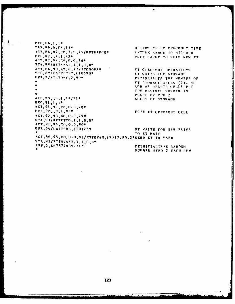
V'A" , ,6 , I'F p 1 5* DFTFR"1'F FT CI'FCKOIIT TIMEA.(T ,46,R7,cn,7.0,7/RFTHAPrE* RFTIIWN RARCF. TO MIC'otlir)PR ,87 ,,7, 1 ,82* FPF.F IPARCF TO SJ'TP NEW FTAC'T,97 ,F4,rnO .O,7fi*'lTA,9AR/!FTVz'AR ,I,1,f,R*AC'T, H6 , '9,AT,6,77/FTcnorS* FT CitEr.OVnilT OI'FRtTIO"S

0 I'r8'~/'A~r~sT, 1O~o* T WAITS FOP STnHArF'~Fqq/FT~r)Ip, ),L~f* FTAlBITrlIFS T'I1' '%'!MP.FR OF* FrT !;TOIRACF CFI.l.S (2). To* A[)[) OR IIFLETE CELLS IT* TI' )FrFIgFn NIIMRFR IN* PLACF OF TPF 2

ALL'C, 90 , , Q , I , t( qIAL T F T R G

ACT,91,92,ro,0.0,78*FR F, 02 , , R, I , R5* FREE ET CIEFCKOUT CULACT, 92 ,93 ,Co O0.0, 79*%TA ,91 /R FTET.O ,l,1,f,R*AXCT, 91.,94, ,O.0, 80*QIJE ,94 /VAI TSIP. ,(1O)73* FT WATTS FOR SRR PRIOR

* TO FT MATE'A(:T, Rn,95 ,Cn, O.O,R1/ETTOVAN,(9)17.FQ.2*SEND ET TO VAFPST4,qS/FTTnVAF!,I ,I,l,II*SFF,2 ,I67574Mlq2/1* REINITIALIFS RANnoM

* NI'MRFR SPED 2 FArjh R1hN

123

*TIIF E".~lTI.INF.S OF CnrF ARF T1IF PAR&MrTEP SEFTS IUS.,n IN*TIIT9 PPOCRAM. TIlE FIRST NtlM1fl,1 %FTri! PAR IS ThIIV PAIIAMFTER*SFT NI'FF. TIIF NEXT NI1NIII.R TS TIIF 405'r 1.1IELY TIME

11' Tl'F lAFTA-PFRT nTSTRIIRIITTON EXCEFPT FOR PARAM.1TFR SFTS 22,*23, Arikv 24, IN 141ITCH CASE THF NtIMRER IS. T4F &1FAN OF A nORMAL *

* lISTPI PH1TTOSP. TIlE. NEXT TWO NPMkRFRq AR P Till' 'ITNYIMIM ANP* 'AXTillI Tri ES F04 THP DISTRTIITTON9. TIIF FOlIRTl N(IMBF1R IN

k '17l1 PAIVI'FTUVH SETS IISINC TIIF NORHIIA1 1 STH(TPlf'T tON I-, TIE* 'TAN11"AHD ')Fl1\ TT0M OF TI ISTHI RwTTNm. ALL (IF TVV F AUAIFS*ARV 11! TINITS OF DAYS.,

PAR,I,7.7O,I.5R,13.83* SJFF hN:DnE~FSERVICF

I1'J!, 2,2.R0,0.4P,5.I2* CAIN "Ill ACCESS1Al1,3,2fln,0.26,1.94* RpmOVE IIORT7.ONTAI. PI,P1AH,4,1 ,40,0. 26,2.54* Rr.IOVV VHT1CI.F rr1.

lA~S,.f ]().1,').to* INSTALL. UORTZONTAI.

PAQ,,6.3),I.8,11O3*CIJFCKOIIT POR'IOMTAL PtI'AR, H,9q *0 ,.1 I ,t.10* INSTAL.L VFRTI(CI.1'

* FI.Irl'T l'TPIAR .1,9.802.1') 17.59* FINAL PIl CIIFCYOIUT

I'V' 10 I ~ 'I), 2* 1,35.0* OLITIMF SSMP MAINTrAR~ I ,OAS?. 1 ,1 r)~ 0 *IIPETP I"SPFCTION

PARP, I',ll). 'j, 2.10,1 R *90* IVOTP I NSPFCTIflI!I.ANR,I1,q.0',7.l0,t4.00* rNC RFMOVE 1% TVSPECT

I'AR, IA,?2.Afl,2.lO,42.70* ROUrTIVE SCIIflnILED* ORRITER LIATNTFNANCF

PAR.15,77.1(l,2.l0,52.50* Pil TCS RrPL.ACFPA4916,7.74,2.10,13.4R* PARTIAL PIP TCF RFPLACFrAP,l7,4.64.2.l0,7.I9* FUIEL CELL RFPLACF1A!,4,.1,1. ,42. AP*TPI RFATNTANCPAI k, I H,l4, 1 , 13,2705* API PLA NFNPA4,241,4.20,1.1,7.09* ORBITTE.1 AATr ACTIVITIESPARl,21,26.hO),2.jO,5j.jO* PAT% OPFRATIONSPAI,?2, I :.WJ),7.(,0.0,83.0O* SpArEL411 MT1SC-ION!,IA,21,4.00,2.f)f,6.00O..O* NOMINAL m1SSION

PIAI,2,3.2',31.00,33.00,O.5* VAPS OHRBTTER OPSI'AI? ,25 ,2 I. 0,1l* 75, 37,45* SPR AFT BITLIMPp1AI',26,4,qft,2*R4,6.96* SRII INTA(:VIThIC OPS

PAp,7,4.nf).,2 .114.6.96* ISIMf C1IfCVOITT ANnA A1. 1 G N11 VN T

IA R 7 4. . 3 H. I. 3 3 ET MATE OPPRATIOUSPA',?',2'.4l, 1.66,411.1,4* SRII/PT rIlPCYOIITI'AR ,1O ,I0.0,4.55,13.25* FT CHECKOUFT OrSFT%!'~*

124&

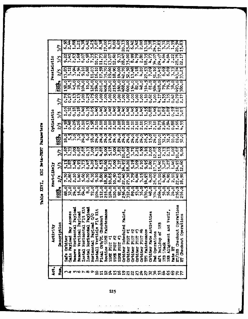
O D 4N .4,. t- 0~0 MO P - - '-4 U, t

%0 N4 W4s. -4 0 n -M ,-O-0 %

. ~ ~ ~ ~ ~ ~ i CZO~ ~ 0 4. 4 ' ~ l %

0 M Z 1 4 1 lz1; t C;- - -- C ' -% OD*-4 O 4~ -4 .4 '' 4 Nv#A N W.,-( 4 - Vq-4 N Cl\-

to a* 0 0 O5lii . I Ct5. . . 5

"q M 1-4 4 U''\~ 00 00 00 0 NV M~ s -Ooo-oaooo-ONC00 0 0 000 '-4 00 V.A',000--

00 4so e 0 0 0 -? c4

0.- C--,4 -\ a

m n v% '*

0 CC 4 -4tC 0 0 0f~ 0 oc -

w4

S 0 CQ NN N-cm-q N-N C4 NI'-4 Nv Wv~4 '~ oC4N 0 U4

N0cl N 00m IN NNC'N N N %N 0m04.4NW40C\ l

0l r0 CV N N Os W%I WN(N Me Nq4C-CY4CN N- C~ "4i.4U0

W44

-rC-0-. 00 C- VIN W-40C.-~~~ '0 v00 v ,' 0C. . 4' 0.O'0

'f S ' CZ C4 4 ': S~c \s d" a, w C; o * -CqL-t-.MA; 0M *NNC(W W "q1400v-* O~ N Cm 4 NN.-V4 N

C4V4W4 Y q-4 V- eq 4 -14 r4-4~

~0

a 4 *.C. P 4 XdJ 4 >

> 0 00 0 0 0 0 0 0 0.0 00 0

e-4 C-44 M U.I 4.E.E 19

V r4 r 4l0 0 b 02- to)=

442).P -$ S) S So 00~v "JPr~j0 "4 4 C3

4S.4 00 00000.I 0 4

C-O %0 N \ $ I H4CdOC INN Cu n0

94 ~ ~ ~ W4 00V O~tt

125

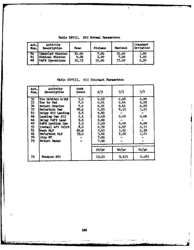
Table XXVII. KSC Normal Parameters

Act. Activity StandardMum. Description Mean Minimum Maximum Deviation

' Spcelab Misr-ion 12.00 7.00 30.00 3.0041 Nominal Mission 4.00 2.00 7.00 1.0048 VAFB Operations 32.35 31.00 33.00 0.20

- ~ _I ____________ _____ ___ ________

Table XXVIII. KSC Conrtant Parameters

Act. Activity WorkNun. Description Hours 2/5 3/5 3/7

30 Tow Orbiter to VAP 1.0 0.09 0.06 0.0433 Tow to Pad 7.0 0.61 0.41 0.2934 Return Crawler 7.0 0.61 0.41 0.2937 Refurbish Pad 78.0 6.83 4.55 3.2513 Delay XSC Landig 9.6 o.Lo - -44 LaMding Ops KsC 1.0 0.09 o.o6 o.o446 Delay VAFB Land 9.6 O.1O - -47 VAFB Landing Ops 1.0 0.09 o.o6 0.04

53 Install Aft Skirt 8.0 0.70 0.47 0.3361 Wash 11P 62.0 5.43 3.62 2.5962 Refurbish MLP 39.0 3.41 2.28 1.6374 ship ST - 7.00 - -

75 Return Barge 7.00

24/yr 40/yr 60/yr

71 Produce ETS 15.21 9.125 6.083

126

a:at :a a: :2 :a :::: a:

NA W~ W4 C14 cm C1 - -

m W (n mY fnC"

I~ zA' A' 2' 'A 2- 2' a 2-

N N(n N mN- N N N m 'N m

WI ' - r\%\uW %fW) D-~ ~W sNC1

CM m N ( n M' m~ Nr% mm

NNNNNNNN N (4N N CM C.J

W. % N.W to q -N OD mWisp R Ch U\,

0 W3 q2 24 N"~ m 3104 2A 2n SM *SA 1 03 4 2 0

V4 W4%J WN9 Yc r

12?

r-4

CW , ,, ,E

r--S

I) N (V N N ~

:C.- L%-

2 22z 2 32 2 : 2 2 %

PC -

P-- El.- L%- C---

Nm M'N M~ NC

3 %0VN~o S L-o SoC%_ No -4:9C

WNE $o.o .0. oSCV4:3 V4 %MV* 0 (1%0 C''0O - CC.111 P - WN R a "IMI 1

128

Appendix B

YAP ?Wdel

This appendix contains the VAf Q-GCRT simulation model. The

graphical model is presented in igure 7, followed by the computer

listing of the Q-CERT program used and the parameters used in the model

(Table XXX).

129

Atw%

0

CC

13

*~

0 1 0-

lip

I IU

400

131iIY

IL))

rz1z]

MIAI

UU1

r~IZ

132i

*THl1q PvlHA!' TI; TIRE. 0-MIlT COV)F FOR A ;TilLATr1On mnDlE1.*TIIAT l)FP'T(:T!* T11E 'LoiJ OF T1lE SPACE TRANSPOHTATTn'J sys.*TEM1 AT VlAVlIFVRFI?r AFH. iiiq mODE!. Is II111 TO PR~nICT THE* IAIINCII HATV CAPA!ITLITY OF TIlF STS AT VAII. TI1. MODE!j.*'4AS PlfSTr'1F1 TO DETERMINE LAIINChO RATE FOP ONLY T11F CON-*FIGURATION if-,Fl) IN TPE MODP., liIOIJVE.R. T1;F IfI;FI CAN ALTFR*TI'E %in!)FI. To FXAfIINF OTHEFR CONFIMIRATIONS oF Till, sysTEM.*TIFF PORTIOM'S THIAT CAN BFP FAvTI Y VARIEDT ARr. TP?! N111P111R OF

n py.ITFPdS, THEI NIMBER OF ORBITTR CIIFCVOIIT AND MAINTENANCE*FACII.TIPS (11MCF), THE NUMBER OF FT CIIFCKOIIT AND STORE-*ACV CELLS, AVMD TIF NUlMRER AND TYPF OF FT RAPGFS lISP! TO*SIP FTS TO VAFH. TIlTS MOin)FT. ASSIJN41S THIAT Til'RF ARE AN* NLIMhITFO NIVIKERl OF FTS AND SRBS AVA] 11.17 TO Tilt SYSTEM.*

I N ADDITTON IT ASSUMES THAT T11FRE IS ONLY 0NF.1 AUNICH PAD.*AS Ah' OuITPulT TilE mOpE!. CIVF DATA !! TPF TPIF K 1.TWF FN *

1 .AITNCI!I'.4 AND THlE STATISTICS ON THIS DATA. TN ADDITION,*TFIF OUITPIT CIVFS STATISTICS ON THEF NUMRER AND A1MOIINT OFl*TVIF TIIAT TRANSACTTONS WATT IN TUEF VARIOUS ()IIFI'PS.

VIUNCTION r'F (IEN)

*TIlTS 1% A FUINCTION PROVTnED BY O'GE.RT T11AT ALLOWS TIlE*I'SFR TO MAKI: tioIFICATTONS To TRANSACTIONS AND ACTIVITIES.**FuINCTION lVF IS CALLED AT NOnF SPECIFIEP BY THE PROGRAMME.R*WITI! TVE ARCf!!MF'4T TFN. VALUES CAI.CIJLATFI) IN THE FUNCO*TION ARE v%;T1RNFT) IN UP. THEF QVAR COMMON RI.ncic CONTAINS*VARITRLFS; PEOI''R El) AND USED BY THlE o-cERT ANALYSIS PRO6* GPAM. FOR A DEFTAILE.D DgSCR'IPTION OF TIIE VARTBLFS SEE* "!IODETINC AND ANALYSIS USTNC, Q-GFRT NFTwRKS, BY A. ALAN* B. PRITS$'ER, PACFS 243-248.

Com,,ION /qVAR/ NDEF,NFTRII(100),NRFL,(100),WIRFIP(100),I NRVT,2(l00),NRUN ,NR!INS ,NTC(l1l) ,PARAM(IlO,4) ,TBE.TNOW

133

*TI'TS PORTION OF THE IuSER FlINCTtON (11F) YR, USED TO DETER-**MINF WHIAT TYPE OF &CTIVITIFS HAVE TO RF ACCOMPLISHED

*WILE I!NLOAI)TNC THm FT RARGE. THIS PMODFl. ARSSUMES TIIAT 4F TS ARF TRANSPOPTEr) ON THE BRGFC AT ONE TIME.. IF THVERE

*APP. NO FTS ON TIIF RARCE THEFN TIlE BARGE IS RETITRN~Fn TO*P1(1' lIP MORF rTS (1fF - 1). IF THEFRE ARE TWO0 FTS LEFT ON**TIIF qARrF, TITER TUEF TRANSPORT STANDS FOR V~IE FIRST TWO* q ARE IOAn)Fn ON THEF BARGE REFOE ANOTHER FT TI'm UnOADED* (IF - ?). IF THEFPF IS nE OR ThTREF FTS STILL OFN THlE BARGE,** THEN4 1'I' NF-VT 'vT 19 IMMEDTATFLY IINLOADED) (IIF -I

IFP (I rN: * *1) THlENTF (%JRFL(5).Fn.n.0) TI'PN

VF- 1.0ELSF IF (Nl-FL(5).FO.2.n) THEP

IF-2.'0

IPF - 3.0FNTn IF

FNP IF

H ETIlR N

*Tt~r l'ol..'INCT IS TJIE 0-CERT CODE 11SF!) To DEPICT THlE (.RAPTI-**IrAT, %inODE OF THF '7AFB SYSTEM. THJIS CODE IS IlgrE! BY THE *

* -rFPT ANALYSTS PROGRAM TO ANALYSE TVHE SYSTEM. TIlE PPO *

*CRA'M ArcCnmItllrFIS 10 RUJNS OF THE SYSTEM, EACI BIiENG 4015**DAYS IN ILPNCHIT. T1HE FIRST 365 DAYS OF EACH RUIN ARE 1C *

*NOREP ANT) NOT USED FOR CALCuTLATING THlE STATISTICS. TI'IS*Is nn.F TO PE.IHCF TIIF POSSIBLE EFFECTS OF TIIE STARTING*CON11TTrONS. AS AN OUTTPUT TIlE PROGRAM PROVTIDES THE RE *

q l'L'rp OF T!Il PNALYSTS, AVERAGE!) OVER TIlE 10 RIUMS. FOR A* DTATI.Fn DESCRIPTION OF THE O-GFRT COMMAND~S UISEI SEE*"monFLINn ANT) ANALYSIS USING 04GFRT NETWORKS", BY ALAN A.

ft.) PRITRICER.

*F , ,~is y~ h np .9,7 lA ,. . .n sl ,3 54

soi)lSitfni ,A* SOURC17 OF FTPqT 4 FTS

ACT,Sl,t,cn,no,,?,(9)A2.[IE.4* CENFPATF FIRST 4 FTSSn011, ,0 1 , A* qOl1R CF FOR -iffi' SUAITENT FTS

ACT,%'2, 52,co,j.n,3,(Q)A3~i~.2q9*ACT, ,.1,cO,1.0,4,(Q)AI.LFP.3nn* GE.NERATE2 300 FTSI)IF,I/FT~IrCl,(Ilo)2* FTS WAIT Fnit BARCEVFS,I/RAR'.F,492* FSTAJILISIIES 4 BARGES

AI.1.?,,l,,I/3*ALLOTS BARCFE TO FT

ACT,,~,t1P%,I,r/'lI~PVAFB* SHIP FT TO VkFRvtiF5/F~vA~,(I()6*FT WATTS TO 11V 1INLOAD~nttFS2/XPHT,1M* STABLISPEFS Ttir NIIMPFR* OF FT TRANSPORTSAf~l,(,,2.1./7*ALLOTS TRANSPORTQI;F7/WATST,(1O8*ET WAITS FOR* STORAGE CELL

RFS,l/RTORAC.F,4 ,6* FSTAB1LISHES 4 FT STORAGE* CELLSAILR,,3 ,,7/~*ALLOTS ET STf)RA(rF

ACT.9,L,NO,2,6/OFFIflAn* OFF LOAD) FT

ACT.I0lII,NO,3,7/XPORrpT* TRANSPORT FT TO STORAGFE

ACT Ii 12NO,,R/CYISP*INITIAL FT INSPECTIOnt

ArT, I2.I3,rn,o(.0~ArT, J?2')2,rn,1) 9H ,1* RFTII-'M XPORT TO i)nOCvO1JI.,1/ :TcroT,(10)14* FT WATTS FOIR CIlF(OIT rFI..

F.R ,4/KITFI,114 STA1RLTSIIFS I C1CI(Ol1T C FT.!.AI.L14 ,4 , , 1 / ~ALLOTS C t'FCKOIIT C F!.I.

ACT.,jf,N.O4,11/CKOTPREP* PRFPARE FT FOR CIIECKOIITRFC.,16,9 ,I*ACT,IlA,17,NO,5,12/FTSYqCO*, CHFCVOI)T FT SYSTEMI; .C. 1 7, 1 ,1*ACT, 17,IP.No~h .13/SEctiRpcn* SP.CIRF ET FROM CIIFCKntUT

R P.C* I , I,115

VA S, 20.1 . 11F I* DE.TERMINE 1,ARGF ACTIVITIPS,ACT, 20 ,21 , 1,,7 i5/-.nrTI~fn,(9)A1.FQ.1* 40 FTS ON RARGF

* LOAD LAST 2 TPAMS-Ar POPT STAXIIS

ACT 2122 ,~n 1 ,6/RmA~A~*PFTIIRN RAR':v TO f1lCIIOt'O)PAF ,? ,,14,*FRFF 4 IRAPGPS'

V:T, 2!,21, GO, ()1,I7*

ACT, 21 'v4, cn, 0 .(, H*

ACT, 20,24 Nn,g I Q/Ti.1NETO (9)A 1 FO. 2* TW.O F'S OM~ BARrCP* LOAD FIRST 2 TRANS-

ACT, 20,14 r,.0~l,20/OT1FRTN(9)Al Eq. 3* 1 OR* i FTS* O1% 1ARCF. NO* SPFC7I.A ACT.

PFF,4,,?,! 'A* FRF.F TRANSPORT

AC? ,?4 , 7', ri,0.0,2j*

STAV25/XPOHTRF.,t,,1 ,%*13Ar-T,IR ,2b,NO , 6,22/PRFPC0* PRF.PE C11FCV11IT CFLL

* FORl NFXT F'rACT,IS,0 6 ,Ot.,2 3/FTTOSTOR* RFTIF'QN FT TO STORArF

rprf,2E6,,4,1,j4* FRFF ET C!F.Cl(01IT CFU.L

AVT,2fi,27 ,CO,o0 0, 24*STA,27/ropFTI ,I , ,ri*

(!IT,2~/T~AI,(1O46*FT 'VA[?S POR USE5031, ~ ,0,I*SO1!RCP OF nOlITER

ACT, 51 ,?q ,rn,0.,44/CFNORH3* GFNFRATF OR'ITTF-!

oil r, 29/n iON El.v AvACT ,24 .1O ,NO *',25/0-AFrnitil ISAFF nRRTTI:N

ACT, 30,1),NO,1fl,26/TOV!OHCF* TOW ORRITFR To nmCr

OIF,31/WAfTOjcr,(10)32* ORBITER 4AITI; FOR OMCPRFq,5/0MCFIkAY,I,32* FSTARLtS1PS I O%1CF HAY

ALI.1?,,,1,1/33*ALLOT nMCF BAYRPFC, 33,1I, I *AC'T,31,34,N,1),I,2710,4CFACT* OMCF ACTIVITIE.S

OttE,,34/O1?%%WATT,(10)35* ORBSITF14 WAITS FOR 1ISP.

136

( ~ ~ L,3~iRYOI.,AS4,()345O*W1EN ROTH1 TH', ORfIITFP*~N A *fl) ' FT/qRft ASSFMRIY

* ARF. tkVAIRBLF TllPN TIIF

ORBITFR HAT~T; PR~O-* CES~S IS RFCIN

ACT, 34 ~ ~ 'ATF OR11ITFR

FI~F37 ,~ ,112 ~FRF.F nMCF RAYAC*T, 37, 3 ,ro,fl.f,3I*

STA , 3/OMCFR Fl.,, *1 ,fl,

A U) l,40, !O,12,3?2/PADOpS* 1,AINC11 PATI OPFRATIONS1;TA 4 n/AINC"1, I , I,D1 * LAITNC11 ORRITFR AND

* RECORr) TTIE 11FTUFN* SU(CCF.SLVE LAfINCUfFS

ArT,4f),41,N,%')13,313/,%IISSION* ORBITE.R MISSITON TIMFntlF,41/I4AITT.AN,04),,(J,(7)42* LANT)INr, OuUU FOR ORBITERr'pFc ,4?~,1, I*

ACT ,42,41,Co, I*0 ,34/DFLAYLAMD* nFlAy LIANi1THC IFS STRI IN I1SF

ACT ,4I ,2Q,NO,14,35/I.ANflOPS* LANDINC OPFRATIONS

AC7T ,4f,4 3,t'O,I5,16/5FCPAl* SPECHRF PAT) FR(W, LAIINCIIQ r4 3 ,1 ) *

ACT r,43 4 4 ,\n , 1 6 137/1,-FFRp,Afl* RM.IRRYBS1I PN1)

AC7T,4.,1,4,Nn,17,'18,slJPPOT RFFRYI* RFFIIPP7ISI, SlIPPORT FITNCitF,44 ,2 2*

ACT,4494,-4o,lp,39/AsgYSR* STACY SRRS ON PADl

nIF,45/RR~llTT,1,(10)4fi* SRII ASSY WAIT% FOR F.T* INITTAL1.Y OnF TV~ OtFUr

SFf. 4 6/ TTng I! rpS'!( 7 ) 452 R UwHEN AN FT A~ln* SR11 ASSY 44P NVAIL'IMF

7MPHN rT MATE 11; RMCIN 1ACT,46,47,cfl,O.35,40* XPORT FT TO PAT)

vFc, 4 7 ., 1*ACT. 4 7.49 H, Cri.n,4 1*11F,4P,,31,A VFE FT STORArFAE:T, 9 '4 Q,ro, 0.0,42*

ArT,47,5n,-:n.l9,4j/?MATFFT* MATF FT TO SRR ASSY

OllF,50)/ASSfYWAT,(10)1%* SRII/FT ASSY WAITS

137

*TUE FO!.OWING ARF TIIF PARAME.TER SETS USFED FOR T11F ACTIV-*ITIES ISFD IN TJ'!S MODlEL. THP FIRST NJUMBER AFTER T1E. PAR*IS T14F PARAME.TER SFT N!JMHFR. PARAMFTER SET I TS FOR A1 Il7TFOR-i DISTRIBUJTION, IN T11I9 PARAMETER SET THE FIRST

*PARAMFTFR IS THE MINIMUM TIME WHlILF T11F SFCO!nD PARAMETER*IS Tirr HAX141111 TIME. THEF RFST OF THE PARA"FTFRS ARE FOR *

*T11F NORMAI. nISTRTBUTTO'N. TH-q FIRST PARAPFTFR I% T4E MEAN*T1lF. , THE S ECOND IS THE MTNIM11M TIME., TIIF THIRD) IS THE *

* IAXI-1'I TIM!1:, ANY) T 1W LAST PARAMETFP 1S THlE STANnARI)D F-~*VlT[fIl. ALLi OF T11F PARAMETERS ARE IN ))AYS.

PAR,],,25.0,30.O* SHIP TIME FOR FTPAkP,2,O).I1,O.(66,O.195,f).022* OFF LOAD FT

rAR,,O.VO,)O~R,.15,O.Ol* FT XPORT TIME AND*F.T INITIAL INSPECTION TIME

P.%R,4,J.(q2%,1.4on,2*450,O*175* PREP FT FOR C!IFCKOI'TPAR,5,2.8O,2.275,3.325,0.175* F.T CHEFCKOIJT TIMEPAUo,,,I.750,t.225,2.275,0.175* SF.CLRFJ FT FROM CIIECK0IITPAR,7,O).416 ,o.ogR,O.744,O.109* LOAD FT TRANqpORT

* STANDS, 0 IN OPTEJEPAR,.U,0.214 ,O.175,0.306,0.022* LOAD FT TRANSPORT

* STANDS, 2 IN nlIFIJEPAR,Q,2.9fl9,1*7q4.4.02,,n.372* SAFr ORRITERrP,\O,O,.1O),uA44..16,0.O6h* To%4 ORR TO OMiCFPAR, l1,i 6.3119,I.675,21.963,1.8l*?ICF ACTIVITY TIMEPAR, 12,6.P47,S.13S,R.156.0.5O3* PAD OPERATIONSI'ARI 3,4.00,2.00,6.OO,1.OO* MISSION TIMEPIAR.14,0. 179,O.n44,0.43P ,O.044* LANDING OPERATIONSPAR,15,fl.I75,0.liO9,f.241..22* SECURE PAD FROM LAUINC"PAR,! 6,4.244 ,2.27S,6. 213,0.656* YIEFIIRBTSII 1,4IINCII PAI,PAvR,1 7,1.fi7,2.8AR,4.463 ,0.263* REFIIRBYSI? SUPPORT FUNCPAR,IR,4.374 ,1.85fl,4.900, 0. 175' STACK SRIIS

PAR,jq,j.400,n.975,1.925,o.I75* ET MATE TIMF

138

C'J'--4 WE* W ONU0% N V4AC *N '. o mU'

.: 000 00000004OW~400000) 0

000~ ) 00 0 0 0 0 0p N -14 0000 CO ON00 t A 9 0O0 0

N 00 NN'.4 NL0-RoN, R0CIJ 0 0

3 1 "!W I c C C 4 0~ ~ C C ' 0 0 0 1. 04 c 90 %

0 0000 NC*4C4N "00N 40 94 N U'.O0 0 C4 N.N

%r S %0UN8ND n8k~ 0 0 "000c 0

CJN cl CN ONO U%8 * VN3

N

N MN NN 0WO% C0 0 - U-% % (

000 - -40 N 0.VN O N V 0l

*00 00C1 I4 N "100 0 %O-I'04 0 0 ~ Os-NI)o

8 0 00 0 0 0 000000OOcp . . 1 0 aa . a . 3 aS00 a a0 -4NN 4 c '. ON V-4

V4NV4 N (1 4 N Nj(I -

r4W4

4- 9 N 04 N c4A444a 44NiNS\

N 1N Nm39N %K.4

VITA

John Gregory Andrusyszyn was born on 9 March, 1953 in Syracuse,

New York. He graduated from Fayetteville-Manlius High School in Manlius,

New York in 1971. He attended Clarkson College of Technology, Potsdam,

New York, from which he received the degree of Bachelor of Science in

Chemistry in May 1975. He entered the Air Force on active duty in

November 1976, and received his commission from Officer Training School

in February 1977. He served as a Space Surveillance Officer with

Detachment 6, 14th Missile Warning Squadron, and then as a Systems

Director and Training Officer with the 7th Missile Warning Squadron,

until entering the School of Engineering, Air Force Institute of

Technology, in June 1981. He is a member of Gamma Sigma Epsilon.

Permanent address, 119 Eureka Dr.

Manlius, New York 13104

la.0

VITA

Brian Grogan Millburn was born in Cleveland, Ohio on 2 April 1953

and he was raised in Missouri. He received a Bachelor of Science

degree in Physics from the University of Missouri at Rolla in May 1975,

and an MBA from the University of Missouri at Columbia in December 1980.

He has been on active duty with the iSAP since April 1976 and was

stationed at Whiteman AFBp, NO until 1981. While at Whiteman AFB,

he served as a Missile Launch Offloer, Missile Flight Commander, and

Emergency War Order Instructor, He was transfered to Wright-Patterson

APB in June 1981 to attend classes at the Air Porce Institute of

Technology (AIT) School of .ngineering, He Is a member of the Initial

class of AF7T's Graduate Program in Space Operations.

Permanent address, 2040 Flamingo Drive

Florissant, MO 63031

UNCLASSIFIEDLCURITV CLASSIFICATION OF THIS PAGE (Whaen Dae. goaters d)

REPORT DOCUMENTATION PAGE BEFORE COMPLETING FORMIREPORT NUMBER GOVT ACC;SO' OS EIIETSCTLGNME

7 7AFIT/GSO/OS/82D-1 AD IO . REIIN AAOGNM0

4. T IT LE (end SubitIle) S YEO EOTAPRO OEE

AN ANALYSIS OF THE SPACE TRANSPORTATIONMSTEISYSTEM LAUNCH RATE CAPABILITIES UTILIZING I. PERFORMING ORG. REPORT NUMBER

Q-GERTSIMULATIONTECHNIQUES______________7. AUTHOR(a) 3. CONTRACT OR GRANT NUMBER(s)

John G. Andrusyszyn , Capt, USAFBrian G. Millburn, Capt, USAF

9. PERFORMING ORGANIZATION NAME AND ADDRESS 10. PROGRAM ELEMENT. PROJECT. TASKAREA & WORK UNIT NUMBERS

Air Force Institute of Technology (APIT-EN)Wright-Patterson AFB, Ohio 45433

I I. CONTROLLING OFFICE NAME AND ADDRE.SS 12. REPORT DATE

December 19821S. NUMBER Of PAGES

____ ___ ___ ___ ___ ___ ____ ___ ___ ___ ___ ___ ___ 152Is. MONITORING AGENCY NAME & ADDRESS(II different from, Controlling Office) 1S. SECURITY CLASS. (of this report)

UnclassifiedIS&. DECL ASSI FI CATION/ DOWNGRADING

SCHEDULE

lb CDISTRP9UTION STATEMENT (of this Report)

Approved for public release; diatribution unlimited.

* 7. DISTRIBUTION STATEMENT (of the abstract mntered In Block 20, if different from Report)

18. StPPLEMENTARY NOTES jfiaved fo Weipi~c releas: IAW APR 190.17.

D&Yn for Resecych and Professional Daelopasatftr Force lnztih.IO ct Tec1'oolcqY (AIC) ~ 9JNl

19. KEY WORDS (Continue on fevors* side it necessry~ and identity by block number)Space Transportation System Sim~lationSpace Shuttle Network AnalysisKennedy Space CenterVandenberg AFBQ-eGERT

20. A yS7RACT (Confirman revee side lifneesami and identify by block number)

'14he Space Transportation System (STS) is being developed by NASA for NASA,DD, and comercial uses National Space Policy dictates that the STS become NASA'iand DoD'gprimary means for launching payloads into orbit. Unfortunately, thecurrent flight manifest saturates STS launch rate capability. Therefore, addi'tional operational funding will be required to increase thirsts of launch. Thisfunding must be applied to those portions of the system which contribute greastesto increasing the system launch rate. This study presents two methods for deter-

(2 mining the system launch rate, identifying the bottlenecks. and develoving aDO I o~ 1473 EDITION OF 'NOV 611IS OBSOLETE

SECURITY CLASS8PICArOu4 Of THIS PACE (Owen Date te0

iiiiiiiiiiiiii i

UNCLASSIFIED

20."(cont.) launch enhancement plan. The analytic method is fairly easilyand quickly accomplished, using the data provided in the NASA Shuttle Turn-around Analysis Report, while the Q-GERT siulation method gives more accurateestimates of the launch rate capability. Plans are presented to show thefacility configurations and flight hardware levels required to achieve variouslaunch rate capabilities at Kennedy Space Center. The capacity of VAFB wasdetermined, but no launch enhancement plan was developed since an increase inthe launch rate would require the obvious duplication of most of the facilities.The method presented can be used on data provided in future STARs.

'p

' OlIUNLASSIl IED

DATE,

FILMED

.OWN

3 83

DTIC