I have a DREAM!

(DIffeRentially PrivatE smart Metering)

Technical report

March 15, 2011

Abstract

This paper presents a new privacy-preserving smart metering system. Our scheme isprivate under the differential privacy model and therefore provides strong and provableguarantees. With our scheme, an (electricity) supplier can periodically collect data fromsmart meters and derive aggregated statistics without learning anything about the ac-tivities of individual households. For example, a supplier cannot tell from a user’s tracewhether or when he watched TV or turned on heating. Our scheme is simple, efficientand practical. Processing cost is very limited: smart meters only have to add noise totheir data and encrypt the results with an efficient stream cipher.

1

Contents

1 Introduction 4

2 Related Work 5

3 The model 63.1 Network model . . . . . . . . . . . . . . . . . . . . . . . . . . . . . . . . . . . 63.2 Adversary model . . . . . . . . . . . . . . . . . . . . . . . . . . . . . . . . . . 73.3 Privacy model . . . . . . . . . . . . . . . . . . . . . . . . . . . . . . . . . . . . 8

4 Objectives 8

5 Building blocks 95.1 Output perturbation: achieving differential privacy . . . . . . . . . . . . . . . 9

5.1.1 Utility definition . . . . . . . . . . . . . . . . . . . . . . . . . . . . . . 105.2 Additively homomorphic encryption . . . . . . . . . . . . . . . . . . . . . . . 10

6 Overview of approaches 116.1 Fully decentralized approach (without aggregator) . . . . . . . . . . . . . . . 116.2 Aggregation with a trusted aggregator . . . . . . . . . . . . . . . . . . . . . . 116.3 Our approach: aggregation without trusted entity . . . . . . . . . . . . . . . . 12

6.3.1 Distributed noise generation . . . . . . . . . . . . . . . . . . . . . . . . 126.3.2 Encryption . . . . . . . . . . . . . . . . . . . . . . . . . . . . . . . . . 13

7 Protocol description 147.1 System setup . . . . . . . . . . . . . . . . . . . . . . . . . . . . . . . . . . . . 147.2 Smart meter processing . . . . . . . . . . . . . . . . . . . . . . . . . . . . . . 147.3 Supplier processing . . . . . . . . . . . . . . . . . . . . . . . . . . . . . . . . . 15

8 Adding robustness 168.1 Sanitization phase extension . . . . . . . . . . . . . . . . . . . . . . . . . . . . 168.2 Encryption phase extension . . . . . . . . . . . . . . . . . . . . . . . . . . . . 16

8.2.1 A naive approach . . . . . . . . . . . . . . . . . . . . . . . . . . . . . . 168.2.2 An advanced approach . . . . . . . . . . . . . . . . . . . . . . . . . . . 17

8.3 Utility . . . . . . . . . . . . . . . . . . . . . . . . . . . . . . . . . . . . . . . . 18

9 Security Analysis 189.1 Deploying malicious nodes . . . . . . . . . . . . . . . . . . . . . . . . . . . . . 189.2 Lying supplier . . . . . . . . . . . . . . . . . . . . . . . . . . . . . . . . . . . . 19

10 Simulation results 2110.1 Available datasets . . . . . . . . . . . . . . . . . . . . . . . . . . . . . . . . . 2110.2 A high-resolution electricity demand model . . . . . . . . . . . . . . . . . . . 2110.3 Adding noise . . . . . . . . . . . . . . . . . . . . . . . . . . . . . . . . . . . . 2110.4 Error and the cluster size . . . . . . . . . . . . . . . . . . . . . . . . . . . . . 21

10.4.1 Random clustering . . . . . . . . . . . . . . . . . . . . . . . . . . . . . 2210.4.2 Consumption based clustering . . . . . . . . . . . . . . . . . . . . . . . 22

2

10.5 Boosting utility by lowering noise . . . . . . . . . . . . . . . . . . . . . . . . . 2410.6 Privacy over multiple slots . . . . . . . . . . . . . . . . . . . . . . . . . . . . . 25

10.6.1 Privacy of appliances . . . . . . . . . . . . . . . . . . . . . . . . . . . . 26

11 Conclusion and Future work 28

A Proof of Theorem 2 (Utility) 30

B Privacy of some ordinary appliances 31

3

1 Introduction

Several countries throughout the world are planning to deploy smart meters in householdsin the very near future. The main motivation, for governments and electricity suppliers, is tobe able to match consumption with generation.

Traditional electrical meters only measure total consumption on a given period of time(i.e., one month or one year). As such, they do not provide accurate information of when theenergy was consumed. Smart meters, instead, monitor and report consumption in intervalsof few minutes. They allow the utility provider to monitor, almost in real-time, consumptionand possibly adjust generation and prices according to the demand. Billing customers byhow much is consumed and at what time of day will probably change consumption habits tohelp matching consumption with generation. In the longer term, with the advent of smartappliances, it is expected that the smart grid will remotely control selected appliances toreduce demand.

Problem Statement: Although smart metering might help improving energy management,it creates many new privacy problems [1]. Smart meters provide very accurate consumptiondata to electricity providers. As the interval of data collected by smart meters decreases,the ability to disaggregate low-resolution data increases. Analyzing high-resolution consump-tion data, Nonintrusive Appliance Load Monitoring (NALM) [14] can be used to identify aremarkable number of electric appliances (e.g., water heaters, well pumps, furnace blowers,refrigerators, and air conditioners) employing exhaustive appliance signature libraries. Re-searchers are now focusing on the myriad of small electric devices around the home such aspersonal computers, laser printers, and light bulbs [18]. Moreover, it has also been shownthat even simple off-the-shelf statistical tools can be used to extract complex usage patternsfrom high-resolution consumption data [19]. This extracted information can be used to pro-file and monitor users for various purposes, creating serious privacy risks and concerns. Asdata recorded by smart meters is lowering in resolution, and inductive algorithms are quicklyimproving, it is urgent to develop privacy-preserving smart metering systems that providestrong and provable guarantees.

Contributions: We propose a privacy-preserving smart metering scheme that guaranteesusers’ privacy while still preserving the benefits and promises of smart metering. Our contri-butions are many-fold and summarized as follows:

• We provide the first provably private and distributed solution for smart metering thatoptimizes utility without relying on a third trusted party (i.e., an aggregator). We wereable to avoid the use of a third trusted party by proposing a new distributed LaplacianPerturbation Algorithm (DLPA).

In our scheme, smart meters are grouped into clusters, where a cluster is a groupof hundreds or thousands of smart meters corresponding, for example, to a quarterof a city. Each smart meter sends, at each sampling period, their measures to thesupplier. These measures are noised and encrypted such that the supplier can computethe noised aggregated electricity consumption of the cluster, at each sampling period,without getting access to individual values. The aggregate is noised just enough toprovide differential privacy to each participating user, while still providing high utility(i.e., the low error). Our scheme is secure under the differential privacy model and

4

therefore provides strong and provable privacy guarantees. In particular, we guaranteethat the supplier cannot retrieve any information about any user consumption, whateverauxiliary information it knows about that user. Our scheme is simple, efficient andpractical. It requires either one or two rounds of message exchanges between a meterand the supplier. Furthermore, processing cost is very limited: smart meters only haveto add noise to their data and encrypt the results with an efficient stream cipher. Finally,our scheme is robust against smart meter failures and malicious nodes. More specifically,it is secure even if α fraction of all nodes of a cluster collude with the supplier, whereα is a security parameter.

• We provide a detailed analysis of the security and performance of our proposal. Thesecurity analysis is performed analytically. The performance, which is evaluated usingthe utility metric, is performed using simulation. We implemented a new electricitytrace generation tool based on [22] which generates one-minute resolution syntheticconsumption data of different households.

2 Related Work

Several papers addressed the privacy problems of smart meters in the recent past [9,19, 1, 2, 3, 21, 15, 12]. However, only a few of them have proposed technical solutions toprotect users’ privacy. In [1, 2], the authors discuss the different security aspects of smartmetering and the conflicting interests among stakeholders. The privacy of billing is consideredin [21, 19]. These techniques uses zero-knowledge proofs to ensure that the fee calculated bythe user is correct without disclosing any consumption data.

Seemingly, the privacy of monitoring the sum consumption of multiple users may besolved by simply anonymizing individual measurements like in [9] or using some mixnet.However, these “ad-hoc” techniques are dangerous and do not provide any real assurances ofprivacy. Several prominent examples in the history have shown that ad-hoc methods do notwork [16]. Moreover, these techniques require an existing trusted third party who performsanonymization. The authors in [3] also perturb the released aggregate with random noise anduse a different model from ours to analyze the privacy of their scheme. However, they do notencrypt individual measurements which means that the added noise must be large enoughto guarantee reasonable privacy. As individual noise shares sums up at the aggregation, thefinal noise makes the aggregate useless. In contrast to this, [12] uses homomorphic encryptionto guarantee privacy for individual measurements. However, the aggregate is not perturbedwhich means that it is not differential private.

The notion of differential privacy was first proposed in [8]. Differential privacy says thatreleasing data using a differentially private algorithm will not increase the adversary’s chanceto infer any information about any users in the dataset. The main advantage of differentialprivacy over other privacy models is that it does not specify the prior knowledge of the adver-sary. Initial works on differential privacy focused on the problem that how a trusted curator(aggregator), who collects all data from users, can differential privately release statistics. Bycontrast, our scheme ensures differential privacy even if the curator is untrusted. Although [7]described protocols for generating shares of random noise which is secure against maliciousparticipants, it requires communication between users and it uses expensive secret sharingtechniques resulting in high overhead in case of large number of users. Similarly, traditionalSecure Multiparty Computation (SMC) techniques [13] [5] also require interactions between

5

users. All these solutions are impractical for resource constrained smart meters where all thecomputation is done by the aggregator and users are not supposed to communicate with eachother.

Two closely related works to ours are [20] and [23]. In [20], the authors propose a schemeto differential privately aggregate sums over multiple slots when the aggregator is untrusted.However, they use the threshold Paillier cryptosystem [11] for homomorphic encryption whichis much more expensive compared to [4] that we use. They also use different noise distributiontechnique which requires several rounds of message exchanges between the users and theaggregator. By contrast, our solution is much more efficient and simple: it requires onlya single message exchange if there are no node failures, otherwise, we need only one extraround. In addition, our solution does not rely on expensive public key cryptography duringaggregation.

A recent paper [23] proposes another technique to privately aggregate time series data.They use a different noise generation method from [20] and ours, but their scheme onlysatisfies the relaxed (ε, δ)-differential privacy definition. Indeed, in their scheme, each nodeadds noise probabilistically which means that none of the nodes add noise with some positiveprobability δ. If this happens, there is a privacy breach. Although δ can be arbitrarily small,this also decreases the utility. By contrast, in our scheme, δ = 0 while ensuring nearly optimalutility. In addition, [23] is not robust against node and communication failures.

3 The model

3.1 Network model

The network is composed of four major parts: the supplier/aggregator, the electrictydistribution network, the communication network, and the users (customers). Every user isequipped with an electricity smart meter, which has two modes of operation: (1) in emergencymode, if the consumption is above a certain threshold, which likely indicates some abnormalevent or failure, data is sent directly to the supplier. In this case, we cannot guarantee privacyas the supplier needs to know the location of the failure to fix it. (2) In the operational mode,each smart meter measures the electricity consumption of the user in every slot with lengthTs, and, using the communication network, sends the measurement to the aggregator at theend of every slot (in practice, Ts is around 1-30 minutes). Note that the communicationand distribution network can be identical (e.g., if we use some PLC technology to transferdata). The motivation behind monitoring the sum consumption of different users is to improveresource management and adjust generation and prices according to the demand.

The measurement of user i in slot t is denoted by Xit . The consumption profile of user i is

described by the vector (Xi1,X

i2, . . .). Privacy directly correlates with Ts; finer-grained samples

means more accurate profile, but also entails weaker privacy. The supplier is interested in the

sum of all measurements in every slot (i.e.,∑N

i=1 Xit

def= Xt). The supplier can either obtain

them from the meters directly, or from a separate aggregator entity who though retrievesthem from the meters, performs the aggregation, and forwards the aggregate to the supplier.

Like in [3], we also assume that smart meters are trusted devices (i.e., tamper-resistant)which can store key materials and perform crypto computations. This realistic assumptionhas also been confirmed in [2]. We further suppose that the supplier knows the average daily

6

consumption of each user. 1

We assume that each node is configured with a private key and gets the correspondingcertificate from a trusted third party. For example, each country might have a third partythat generates these certificate and can additionally generate the “supplier” certificates tosupplier companies [2]. As in [2], we also assume that public key operations are employedonly for initial key establishment, probably when a meter is taken over by a new supplier, andafter that, all communication is protected by symmetric crypto-based techniques. Messagesexchanged between the supplier and the meters are authenticated using pairwise MACs.

Smart meters are assumed to have bidirectional communication channel (using some wire-less or PLC technology) with the supplier and/or the aggregator, but the meters cannot com-municate with each other. Finally, we assume that nodes may (randomly) fail, and in thesecases, cannot send their measurements to the aggregator/supplier. This can be caused by de-vice or communication failures. However, nodes are supposed to use some reliable transportprotocol to overcome the transient failures of the channel.

Finally, we note that smart meters also allow the supplier to perform fine-grained billingbased on time-dependant variable tariffs. Here, we are not concerned with the privacy andsecurity problems of this service. Interested readers are referred to [21, 19].

3.2 Adversary model

In general, the objective of the adversary is to infer detailed information about householdactivity (e.g, how many people are in home and what they are doing at a given time). Inorder to do that, it needs to extract complex usage patterns of appliances which includes thelevel of power consumption, its periodicity, and its duration. It has been shown in [19] thatdifferent data mining techniques can be easily applied to a raw consumption profile to obtainthis information.

In terms of its capability, we distinguish three types of adversary. The first is the a honest-but-curious (HC) adversary, who attempts to obtain private information about a user, butit follows the protocol faithfully and do not provide false information [19]. It only uses the(non-manipulated) collected data.

The dishonest-but-non-intrusive (DN) adversary may not follow the protocol correctlyand is allowed to provide false information to manipulate the collected data. Some users canalso be malicious and collude even with the supplier to collect information about honest users.However, the DN adversary is not allowed to access and modify the distribution network tomount attacks. For instance, it cannot install any extra hardware in the distribution networkto collect more information about users.

In addition to the DN adversary, the strongest dishonest-and-intrusive (DI) adversary caninvade the distribution network and modify it to gather more information about users. Itcan access the network infrastructure and, e.g., monitor the consumption on every power lineoutside the users’ households by installing extra meters.

For all cases, we suppose that the adversary can have any kind of extra knowledge abouthonest users, beyond the legitimately collected data, which might help to infer private infor-

1e.g., at the end of every longer period with length Tp, where Ts ≪ Tp and Tp is around a few month, eachmeter sends the real consumption aggregated over the last Tp/Ts slots directly to supplier. This assumptiondo not entail more privacy risks than the old-fashioned traditional metering technique used nowadays.

7

mation about them. For instance, it can observe their daily habits and their other activities2,or obtain extra information by doing personal interviews, surveys, etc.

3.3 Privacy model

We use differential privacy [8] that models the adversary described above. In particular,differential privacy guarantees that a user’s privacy should not be threatened substantiallymore if he provides his measurement to the supplier regardless what external knowledge thesupplier has. Intuitively, a sanitization algorithm is differential private, if any single user’sdata changes the distribution of its output insignificantly, and hence, the output practicallydoes not leak any information about any user’s data.

Definition 1 (ε-differential privacy) An algorithm A is ε-differential private, if for alldata sets D1 and D2, where D1 and D2 differ in at most a single user, and for all subsets ofpossible answers S ⊆ Range(A),

P (A(D1) ∈ S) ≤ eε · P (A(D2) ∈ S)

Differential private algorithms produce indistinguishable outputs for similar inputs (moreprecisely, differing by a single entry), and thus, the modification of any single user’s data inthe dataset (including its removal or addition) changes the probability of any output only upto a multiplicative factor eε. The parameter ε allows us to control the level of privacy. Lowervalues of ε implies stronger privacy, as they restrict further the influence of a user’s data on theoutput. Note that differential privacy does not make any assumptions about the adversary’scomputational power and its external knowledge about the dataset. For instance, this modelguarantees privacy for a user even if all other users’ data is known to the adversary (e.g.,it knows all measurements comprising the aggregate except the target user’s) independentlyof what extra knowledge it has about the user beyond the sanitized data. In our adversarymodel, this is equivalent to the case when N − 1 out of N users are malicious and cooperatewith the supplier.

The definition of differential privacy also maintains a composability property : the compo-sition of differential private algorithms remains differential private and their ε parameters areaccumulated. In particular, a protocol having t rounds, where each round is individually εdifferential private, is itself t · ε differential private.

4 Objectives

Our goal is to develop a practical scheme that preferably does not introduce more privacyrisks for users than traditional metering systems while retaining the benefits of smart meters.More specifically, the scheme should be

• differentially private: Considering DN adversary, the scheme differential privatelyreleases sanitized aggregates Xt where the leaked private information about users ismeasured by ε.

• robust and easily configurable: It tolerates (random) node failures.

2Similarly to monitoring neighbors. Indeed, neighbors can also be malicious users, which is included in ourmodel.

8

• efficient : It has low overhead which includes low computation load on smart meters, andlow communication overhead between the supplier and individual meters. It should usepubic key operations only for initial key establishment. Afterwards, all communicationis protected using more efficient symmetric crypto-based techniques.

• distributed : Besides a certificate authority, the protocol does not require any trustedthird party such as a trusted aggregator as in [3]. The smart meters communicatedirectly with the supplier.

• useful for the supplier : The sanitized and the original (non-sanitized) aggregate shouldbe “similar”. This sanitized data should also be sufficient for the supplier to accom-plish its desired goals. For instance, this includes the supplier’s ability to performefficient management of the resource: to monitor the consumption at the granularityof a maximum few hundred households, and to detect consumption peaks or abnormalconsumption.

5 Building blocks

5.1 Output perturbation: achieving differential privacy

Let’s say, we want to release the value of a function f applied on our dataset in a differentialprivate way. The following theorem says that we can achieve differential privacy by releasingthe perturbed output of f ; simply adding a random noise to the value of f before releasingthat, where the noise distribution is carefully calibrated to the global sensitivity of f , resultsin ε-differential privacy. The global sensitivity of a function is the maximum ”change” in thevalue of the function when its input differs in a single entry. For instance, if f is simply thesum of all measurements, then the sensitivity is the maximum value that a measurement canhave.

Theorem 1 ([8]) For all f : D → Rr, the following mechanism A is ε-differential private:

A(D) = f(D) + L(S(f)/ε), where L(S(f)/ε) is an independently generated random variablefollowing the Laplace distribution and S(f) denotes the global sensitivity of f3.

In particular, if each time the noise is drawn independently from the same Laplace dis-

tribution with PDF P (L(λ) = x) = 12λe−

|x|λ , we obtain that P (A(D1)=z)

P (A(D2)=z) = P (L(λ)=z−f(D1))P (L(λ)=z−f(D2)) ≤

e−||f(D1)||1+||f(D2)||1

λ ≤ e||f(D1)−f(D2)||1/λ ≤ eS(f)/λ for all z. This perturbation method is alsocalled as LPA (Laplacian Perturbation Algorithm).

ε-differential privacy guarantees a global ε bound to all users, as the noise is calibrated tothe global sensitivity S(f). In the sequel, we distinguish an individual’s indistinguishability asfollows. Let D1 and D2 differ only in user U ’s data. Then, the upper bound e||f(D1)−f(D2)||1/λ

on P (A(D1)∈S)P (A(D2)∈S) (for all D1,D2, and S) represents U ’s indistinguishability, where ε = ||f(D1)−

f(D2)||1/λ is U ’s individual privacy bound. In the rest, if it is ambiguous in the given context,we distinguish global ε bound from an individual’s ε bound. As e||f(D1)−f(D2)||1/λ ≤ eS(f)/λ,the maximum of the individual bounds in the dataset is the global ε bound.

3Formally, let f : D → Rr, then the global sensitivity of f is S(f) = max ||f(D1)− f(D2)||1, where D1 and

D2 differ in a single entry and || · ||1 denotes the L1 distance.

9

Example 1 To illustrate these definitions, consider a mini smart metering application, whereusers U1, U2, and U3 need to send the sum of their measurements in three consecutive slots.The measurements of U1, U2 and U3 are (X1

1 = 100,X12 = 300,X1

3 = 200), (X21 = 250,X2

2 =400,X2

3 = 350), and (X31 = 50,X3

2 = 150,X33 = 200), resp. The nodes want differential

privacy for the released sum with a global ε = 0.5 bound. Based on Theorem 1, they need toadd L(λ =

∑

t maxi Xit/0.5 = 2000) noise to the released sum in each slot. The individual ε

bound of U1 is∑

t X1t /λ = 0.3, and similarly, 0.5 of U2, and 0.2 of U3. Another interpretation

is that U1 has ε1 = X11/λ = 0.05, ε2 = X1

2/λ = 0.15, and ε3 = X13/λ = 0.1 privacy in each

individual slot, and ε = ε1 + ε2 + ε3 = 0.3 considering all three slots following from thecomposition property of differential privacy.

5.1.1 Utility definition

Let f : D → R. In order to measure the utility, we quantify the difference betweenf(D) and its perturbed value (i.e., f(D) = f(D) + L(λ)) which is the error introduced byLPA. A common scale-dependant error measure is the Mean Absolute Error (MAE), whichis E|f(D)− f(D)| in our case. However, the error should be dependent on the non-perturbedvalue of f(D); if f(D) is greater, the added noise becomes small compared to f(D) whichintuitively results in better utility. Hence, we rather use a slightly modified version of ascale-independent metric called Mean Absolute Percentage Error (MAPE), which shows theproportion of the error to the data, as follows.

Definition 2 (Error function) Let Dt ∈ D denote a dataset in time-slot t. Furthermore,

let δt = |f(Dt)−f(Dt)|f(Dt)+1 (i.e., the value of the error in slot t). The error function is defined as

µ(t) = E(δt). The expectation is taken on the randomness of f(Dt). The standard deviationof the error is σ(t) =

√

Var (δt) in time t.

Compared to the original definition of MAPE (i.e., E(|f(Dt) − f(Dt)|/f(Dt))) we add 1to the denominator in order to avoid the case when it is zero and to bound the error value.Note that if f(Dt) ≫ 1, then there is no significant difference between the value of µ(t) andMAPE, which is the case for most practical applications.

Example 2 Continuing Example 1, f(D1) =∑

i Xi1 + L(λ), where λ = 2000. Moreover,

µ(1) = E

(

|f(D1)−f(D1)−L(λ)|f(D1)+1

)

= E|L(λ)|f(D1)+1 = λ

f(D1)+1 which is about 4.98 in the specific exam-

ple. Similarly, µ(2) = 2000/851 ≈ 2.35 and µ(3) ≈ 2.66 (i.e., the released sums are practically

useless). In addition, σ(t) =

√Var |L(λ)|

f(D1)+1 =

√E|L(λ)|2−(E|L(λ)|)2

f(D1)+1 = λf(D1)+1 = µ(t). In order to

increase utility, we can decrease privacy. For instance, suppose we want to guarantee a globalε = 0.5 bound in individual slots instead of during three slots. This means that we need toadd noise λ = maxi X

it/0.5 in slot t (instead of

∑

t maxi Xit/0.5) which means that µ(1), µ(2),

µ(3) change to 0.62, 0.47, and 0.53, resp. Although these are still not satisfactory, we canfurther decrease the error by taking the sum of more measurements (i.e., including more than3 users into the aggregation).

5.2 Additively homomorphic encryption

A homomorphic encryption scheme allows arithmetic operations to be performed on ci-phertexts. They are especially useful in scenarios where someone who does not have decryp-tion keys needs to perform arithmetic operations on a set of ciphertexts. Let Enc() denote a

10

probabilistic encryption scheme. Let M be the message space and C the ciphertext space suchthat both of them are groups under the addition operation. Enc() is an additive-homomorphicencryption scheme if for any instance Enc() of the encryption scheme, given c1 = Enck1(m1)and c2 = Enck2(m2), there exists a key k such that

c1 + c2 = Enck(m1 + m2)

In other words, the result of adding plaintext values may be obtained by decrypting thesum of the corresponding encrypted values. A simple and practical additively homomorphicencryption technique, which suits perfectly for privacy-preserving additive aggregation, is theCaTsMy scheme [4]:

Encryption: Let k be a randomly generated keystream, where k ∈ [0,∆ − 1]. After rep-resenting message m as integer m ∈ [0,∆ − 1] where ∆ is a large integer, computec = Enc(m,k,∆) = m + k (mod ∆)

Decryption: Dec(c, k,∆) = c − k (mod ∆)

Addition of ciphertexts: Let c1 = Enc(m1, k1,∆) and c2 = Enc(m2, k2,∆). For k = k1 +k2, Dec(c1 + c2, k,∆) = m1 + m2.

This scheme uses modular addition (+) and ensures if c1 = Enc(m1, k1,∆) and c2 =Enc(m2, k2,∆) then c1 + c2 = Enc(m1 + m2, k1 + k2,∆). If n different ciphertexts are addedand p = max(mi) then ∆ should be selected as ∆ = 2⌈log2(p·n)⌉.

6 Overview of approaches

Our task is to enable the supplier to calculate the sum of maximum N measurements (i.e.,∑N

i=1 Xit = Xt in all t) coming from N different users while ensuring ε-differential privacy for

each user. This is guaranteed if the supplier can only access Xt +L(λ(t)), where L(λ(t)) 4 isthe laplace noise calibrated to ε as it has been described in Section 5.1. There are (at least)3 possible approaches to do this which are detailed as follows.

6.1 Fully decentralized approach (without aggregator)

Our first attempt is that each user adds some noise to its own measurement, where thenoise is drawn from a Laplace distribution. In particular, each node i sends the value ofXi

t +L(λ) directly to the supplier in time t. It is easy to see that ε is guaranteed to all users,but in fact the final noise added to the aggregate (i.e.,

∑Ni=1 L(λ)) is N times larger than

L(λ), and hence, the error is µ(t) = 1Xt+1E|∑N

i=1 L(λ)| = N ·λXt+1 . This means that µ(t) can be

large.

6.2 Aggregation with a trusted aggregator

Our second attempt can be to aggregate the measurements of some users, and send theperturbed aggregate to the supplier. In particular, nodes are grouped into N sized clustersand each node of a cluster sends its measurement Xi

t to the (trusted) cluster aggregator, that

4We will use the notation λ instead of λ(t) if the dependency on time is obvious in the context.

11

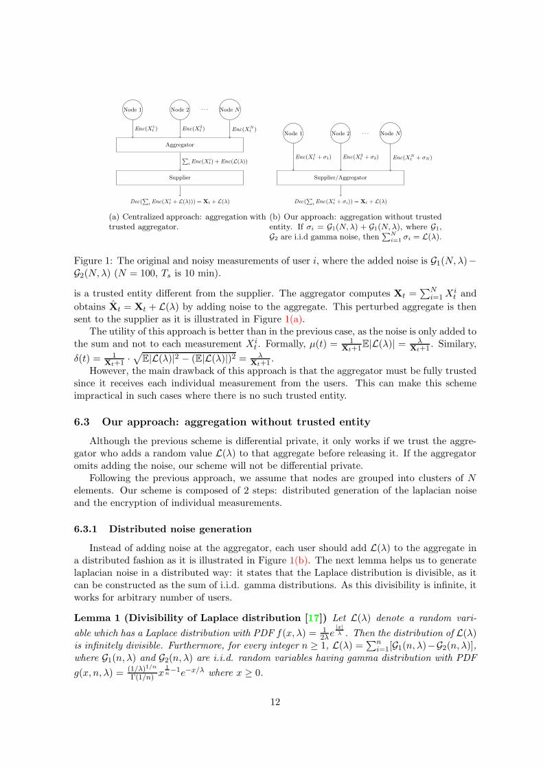
Node 1 Node 2 . . . Node N

Aggregator

Supplier

Dec(P

i Enc(Xit + L(λ))) = Xt + L(λ)

P

i Enc(Xit) + Enc(L(λ))

Enc(X1t ) Enc(X2

t ) Enc(XNt )

(a) Centralized approach: aggregation withtrusted aggregator.

Node 1 Node 2 . . . Node N

Supplier/Aggregator

Dec(P

i Enc(Xit + σi)) = Xt + L(λ)

Enc(X1t + σ1) Enc(X2

t + σ2) Enc(XNt + σN)

(b) Our approach: aggregation without trustedentity. If σi = G1(N, λ) + G1(N, λ), where G1,G2 are i.i.d gamma noise, then

PNi=1 σi = L(λ).

Figure 1: The original and noisy measurements of user i, where the added noise is G1(N,λ)−G2(N,λ) (N = 100, Ts is 10 min).

is a trusted entity different from the supplier. The aggregator computes Xt =∑N

i=1 Xit and

obtains Xt = Xt + L(λ) by adding noise to the aggregate. This perturbed aggregate is thensent to the supplier as it is illustrated in Figure 1(a).

The utility of this approach is better than in the previous case, as the noise is only added tothe sum and not to each measurement Xi

t . Formally, µ(t) = 1Xt+1E|L(λ)| = λ

Xt+1 . Similary,

δ(t) = 1Xt+1 ·

√

E|L(λ)|2 − (E|L(λ)|)2 = λXt+1 .

However, the main drawback of this approach is that the aggregator must be fully trustedsince it receives each individual measurement from the users. This can make this schemeimpractical in such cases where there is no such trusted entity.

6.3 Our approach: aggregation without trusted entity

Although the previous scheme is differential private, it only works if we trust the aggre-gator who adds a random value L(λ) to that aggregate before releasing it. If the aggregatoromits adding the noise, our scheme will not be differential private.

Following the previous approach, we assume that nodes are grouped into clusters of Nelements. Our scheme is composed of 2 steps: distributed generation of the laplacian noiseand the encryption of individual measurements.

6.3.1 Distributed noise generation

Instead of adding noise at the aggregator, each user should add L(λ) to the aggregate ina distributed fashion as it is illustrated in Figure 1(b). The next lemma helps us to generatelaplacian noise in a distributed way: it states that the Laplace distribution is divisible, as itcan be constructed as the sum of i.i.d. gamma distributions. As this divisibility is infinite, itworks for arbitrary number of users.

Lemma 1 (Divisibility of Laplace distribution [17]) Let L(λ) denote a random vari-

able which has a Laplace distribution with PDF f(x, λ) = 12λe

|x|λ . Then the distribution of L(λ)

is infinitely divisible. Furthermore, for every integer n ≥ 1, L(λ) =∑n

i=1[G1(n, λ)−G2(n, λ)],where G1(n, λ) and G2(n, λ) are i.i.d. random variables having gamma distribution with PDF

g(x, n, λ) = (1/λ)1/n

Γ(1/n) x1n−1e−x/λ where x ≥ 0.

12

The lemma comes from the fact that L(λ) can be represented as the difference of twoi.i.d exponential random variables with rate parameter 1/λ. Moreover,

∑ni=1 G1(n, λ) −

∑ni=1 G2(n, λ) = G1(1/

∑ni=1

1n , λ) − G2(1/

∑ni=1

1n , λ) = G1(1, λ) − G2(1, λ) due to the sum-

mation property of the gamma distribution5. Here, G1(1, λ) and G2(1, λ) are i.i.d exponentialrandom variable with rate parameter 1/λ which completes the argument.

Our distributed sanitization algorithm is simple; user i calculates value Xit = Xi

t +G1(N,λ) − G2(N,λ) in slot t and sends it to the aggregator, where G1(N,λ) and G2(N,λ)denote two random values independently drawn from the same gamma distribution. Now, ifthe aggregator sums up all values received from the N users of a cluster, then

∑Ni=1 Xi

t =∑N

i=1 Xit +

∑Ni=1[G1(N,λ) − G2(N,λ)] = Xt + L(λ) based on Lemma 1.

6.3.2 Encryption

The previous step is not enough to guarantee privacy as only the sum of the measurements(i.e., Xt) is differential private but not the individual measurements. In particular, theaggregator has access to Xi

t , and even if Xit is noisy, G1(N,λ)−G2(N,λ) is usually insufficient

to provide reasonable privacy for individual users if N ≫ 1. This is illustrated in Figure 2,where an individual’s noisy and original measurements slightly differ.

-500

0

500

1000

00:00 02:00 04:00 06:00 08:00 10:00 12:00 14:00 16:00 18:00 20:00 22:00 00:00

Ene

rgy

(Wh)

Time

original data

(a) Xit

-500

0

500

1000

00:00 02:00 04:00 06:00 08:00 10:00 12:00 14:00 16:00 18:00 20:00 22:00 00:00

Ene

rgy

(Wh)

Time

noisy data

(b) Xit + G1(N, λ) − G2(N, λ)

Figure 2: The original and noisy measurements of user i, where the added noise is G1(N,λ)−G2(N,λ) (N = 100, Ts is 10 min).

To address this problem, each contribution is encrypted using an additive homomorphicscheme such that the aggregator can only decrypt the sum of the individual values, and cannotaccess any of them.

It is easy to see that the utility of this scheme is identical to the utility in Section 6.1,and thus, it is optimal. In particular, µ(t) = 1

Xt+1E|Xt −Xt +∑n

i=1[G1(N,λ) − G2(N,λ)]| =E|L(λ)|Xt+1 = λ

Xt+1 , and δ(t) = λXt+1 .

Finally, note that using our approach the aggregator and the supplier do need to beseparate entities. The supplier can even play the role of the aggregator, as the encryptionprevents it to access individual measurements, and the distributed generation of the noiseensures that it cannot manipulate the noise to remove the differential privacy guarantee ofindividuals.

5The sum of i.i.d. gamma random variables follows gamma distribution (i.e.,Pn

i=1 G(ki, λ) =G(1/

Pni=1

1ki

, λ)).

13

7 Protocol description

7.1 System setup

In our scheme, nodes are grouped into clusters of size N , where N is a parameter. Theprotocol requires the establishment of pairwise keys between each pair of the nodes inside acluster that can be done by using traditional Diffie-Hellman key exchange [6] as follows:

1. When a node vi is installed, it provides a self-signed DH component gci (mod p) andits certificate Certi to the supplier, where ci is kept secret by vi and g, p are public DHparameters.

2. Once all the nodes of a cluster are installed, or a new node is deployed, the supplierbroadcasts the list of (idi, g

ci (mod p),Certi) (1 ≤ i ≤ N), where idi is the identity ofnode vi.

3. Finally, each node vi of the cluster can compute a pairwise key Ki,j shared with anyother node vj by computing gci·cj (mod p). Note that no communication is requiredbetween vi and vj.

7.2 Smart meter processing

Each node vi sends at time t its periodic measurement, Xit , to the supplier as follows:

Phase 1 (Data sanitization): Node vi calculates value

Xit = Xi

t + G1(N,λ) − G2(N,λ) (1)

where G1(N,λ) and G2(N,λ) denote two random values independently drawn from thesame gamma distribution and N is the cluster size.

Phase 2 (Data encryption): Each noisy data Xit is then encrypted using the CaTsMy

homomorphic encryption scheme into Enc(Xit). The following extension is then applied:

Each node, vi, selects ℓ other nodes randomly, such that if vi selects vj , then vj alsoselects vi. Afterwards, both nodes generate a common dummy key k from their pairwisekey Ki,j ; vi adds k to Enc(Xi

t) and vj adds −k to Enc(Xjt ). As a result, the aggregator

cannot decrypt the individual ciphertexts (it does not know the dummy key k). However,it adds all the ciphertexts of a given cluster, the dummy keys cancel out and it retrievesthe encrypted sum of the (noisy) contributions. The more formal description is asfollows:

1. node vi selects some nodes of the clusters randomly (we call them participatingnodes) using a secure pseudo random function (PRF) such that if vi selects vj, thenvj also selects vi. In particular, vi selects vj if mapping PRF (Ki,j , r1) to a valuebetween 0 and 1 is less or equal than w

N−1 , where r1 is a public value changing ineach slot. The PRF can be implemented using a stream cipher, such as RC4 (likein [4]). We denote by ℓ the number of selected participating nodes, and indi[j] (forj = 1, . . . , ℓ) denotes the index of the ℓ nodes selected by node vi. Note that, forthe supplier, the probability that vi selects vj is w

N−1 as it does not know Ki,j. Theexpected value of ℓ is w.

14

2. vi computes for each of its ℓ participating nodes a dummy key. A dummy keybetween vi and vj is defined as dkeyi,j = (i − j)/|i − j| · PRF (Ki,j , r2) (mod ∆),where Ki,j is the key shared by vi and vj , and r2 6= r1 is public value changing ineach slot. Note that dkeyi,j = −dkeyj,i.

3. vi then computes Enc(Xit) = Xi

t + K ′i +

∑ℓj=1 dkeyi,indi[j] (mod ∆), where

K ′i ∈ [0,∆ − 1] is the keystream shared by vi and the aggregator, and ∆ is a large

integer. Note that ∆ must larger than the sum of all contributions (i.e., finalaggregate) plus the laplacian noise.6 In practice, if p = maxt,i(X

it) (which can be

easily estimated in advance) then ∆ should be selected as ∆ = 2⌈log2(p·N)⌉.

Note that Xit is encrypted multiple times: it is first encrypted with the keystream

K ′i and then with several dummy keys. K ′

i is needed to prevent an eavesdropper torecover Xt, and can be established using the DH protocol as above. In particular,if the eavesdropper knows all Xi

t and they does not contain K ′i, then summing

them up the dummy keys cancel out and Xt is obtained. The dummy keys areneeded to prevent the aggregator (supplier) from retrieving Xi

t .

Enc(Xit) is then sent to the aggregator (supplier).

7.3 Supplier processing

Phase 1 (Data aggregation): At each epoch, the supplier aggregates the N measurementsreceived from the cluster smart meters by summing them, and obtains

Enc(Xt) =

N∑

i=1

Enc(Xit)

based on the homomorphic property of the encryption. In particular,

Enc(Xt) =N∑

i=1

(Xit + K ′

i) +N∑

i=1

ℓ∑

j=1

dkeyi,indi[j] (mod ∆)

where∑N

i=1

∑ℓj=1 dkeyi,indi[j] = 0 because dkeyi,j = −dkeyj,i. Hence,

Enc(Xt) =

N∑

i=1

(Xit + K ′

i) =

N∑

i=1

Enc(Xit)

Phase 2 (Data decryption): The aggregator then decrypts the aggregated value by sub-stracting the sum of the node’s keystream, and retrieves the sum of the noisy measures:

Dec(Xt) =

N∑

i=1

Enc(Xit) −

N∑

i=1

K ′i =

N∑

i=1

Xit (mod ∆)

where∑N

i=1 Xit =

∑Ni=1 Xi

t +∑N

i=1 G1(N,λ) −∑Ni=1 G2(N,λ) =

∑Ni=1 Xi

t + L(λ)based on Lemma 1.

6Note that the noise is a random value from an infinite domain and this sum might be larger than ∆.However, choosing sufficiently large ∆, the probability that the sum exceeds M can be made arbitrary smalldue to the exponential tail of the Laplace distribution.

15

The main idea of the scheme is that the aggregator is not able to decrypt the individualencrypted values because it does not know the dummy keys. However, by adding the differentencrypted contributions, dummy keys cancel each other and the aggregator can retrieve thesum of the plaintext. The resulting plaintext is then the perturbed sums of the measurements,where the noise ensures the differential privacy of each user.

8 Adding robustness

We have assumed so far that all the N nodes of a cluster participated in the protocol.However, it might happen that, for several different reasons (e.g., node or communicationfailures) some nodes are not able to participate in each epoch. This would have two effects:first, security will be reduced since the sum of the noise added by each node will not beequivalent to L(λ). Hence, differential privacy may not be guaranteed. Second, the aggregatorwill not be able to decrypt the aggregated value since the sum of the dummy keys will notcancel out.

In this section, we extend our scheme to resist node failures. We propose a scheme whichresists the failure of up to M out of N nodes, where M is a configuration parameter. We willstudy later the impact of the value M on the scheme performance.

8.1 Sanitization phase extension

In order to resist the failure of M nodes, each node should add the following noise to theirindividual measurement: G1(N − M,λ) − G2(N − M,λ). Note that

∑N−Mi=1 [G1(N − M,λ) −

G2(N − M,λ)] = L(λ). Therefore, this sanitization algorithm remains differential private, ifat least N −M nodes participate in the protocol. Note that in that case each node adds extranoise to the aggregate in order to ensure differential privacy even if less than M nodes fail tosend their noise share to the aggregator.

8.2 Encryption phase extension

8.2.1 A naive approach

As described previously, all the dummy keys cancel out at the aggregator. However, thisis not the case if not all the nodes participate in the protocol. In order to resist the failure ofnodes, one can extend the encryption scheme with an additional round where the aggregatorasks the participating nodes of non-responding nodes to send the missing dummy keys:

1. Once the aggregator received all contributions, it broadcasts the ids of the non-responding nodes. Note that the aggregator knows which nodes are inside cluster,and each node vi should also attach idi to its encrypted measurement which is sent tothe aggregator.

2. Upon the reception of this message, each node vi verifies whether any of the ids in thebroadcast message are in its participating node list (i.e., it can be found in indi). Foreach of such id, the node sends the corresponding dummy key to the aggregator.

3. The aggregator then subtracts all received dummy key from Enc(Xt) and retrieves∑N

i=1(Xit + K ′

i) which can be decrypted.

16

This approach has a severe problem: if the aggregator is untrusted, it can easily retrievethe measurement of a vi: broadcasting its id in Step 2, the participating nodes of vi replywith the dummy keys of vi which can be removed from Enc(Xi

t). In particular, summing upthe dummy keys coming from the participating nodes, the supplier obtains

∑ℓj=1 dkeyi,indi[j].

Then, subtracting that and K ′i from the encrypted value of vi: Enc(Xi

t)−∑ℓ

j=1 dkeyi,indi[j] −K ′

i = Xit .

8.2.2 An advanced approach

In the naive approach, the aggregator needs the dummy keys themselves in order to removethem from the aggregate, but this also enables it to remove that from the node’s encryptedvalue. In the following more advanced approach, each node adds a secret random value to itsencrypted value before releasing it in the first round. This is needed to prevent the adversaryto recover the noisy measurement through combining different messages of the nodes. Then,in the second round when the aggregator asks for the missing dummy keys, every node revealsits random keys along with the missing dummy keys that it knows:

1. Each node vi sends

Enc(Xit) = Xi

t + K ′i +

ℓ∑

j=1

dkeyi,indi[j] + Ci (mod ∆)

where Ci is the secret random key of vi generated randomly in each round.

2. After receiving all measurements, the aggregator asks all nodes for their random keysand the missing dummy keys through broadcasting the id of the non-responding nodes.

3. Each node vi verifies whether any ids in this broadcast message are in its participatingnode list, where the set of the corresponding participating nodes is denoted by S. Then,vi replies with

∑

j∈S dkeyi,indi[j] + Ci (mod ∆).

4. The aggregator subtracts all received values from Enc(Xt) which results in∑N

i=1(Xit +

K ′i), as the random keys as well as the dummy keys cancel out.

Note that as the supplier does not know the random keys, it cannot remove them fromany messages but only from the final aggregate; adding each node’s response to the aggregateall the dummy keys and secret random keys cancel out and the supplier obtains Xt. Althoughthe supplier can recover vi’s measurement if it knows vi’s participating nodes (the suppliersimply asks for all the dummy keys of vi in the second round and subtracts vi’s response fromits own encrypted value sent in the first round), we will show later that this probability canbe made practically small by adjusting w and N correctly.

Note that the protocol fails if, for some reasons, a node does not send its random key tothe aggregator (as only the node itself knows its random key, it cannot be reconstructed byother parties). However, it is very unlikely that a node between the two rounds fails, and anunderlying reliable transport protocol helps to overcome communication errors.

Finally, also note that this random key approach always requires two rounds of commu-nication (even if the aggregator receives all encrypted values correctly in the first round), asthe random keys are needed to be removed from Enc(Xt) in the second round.

17

8.3 Utility

If all N nodes participate in the protocol, the added noise will be larger than L(λ) whichis needed to ensure differential privacy. In particular,

∑Ni=1[G1(N −M,λ)−G2(N −M,λ)] =

L(λ)+∑M

i=1[G1(N −M,λ)−G2(N −M,λ)], where the last summand is the extra noise neededto tolerate the failure of maximum M nodes. Clearly, this extra noise increases the error if allN nodes operate correctly and add their noise shares faithfully. In what follows, we calculatethe error and its standard deviation if we add this extra noise to the aggregate.

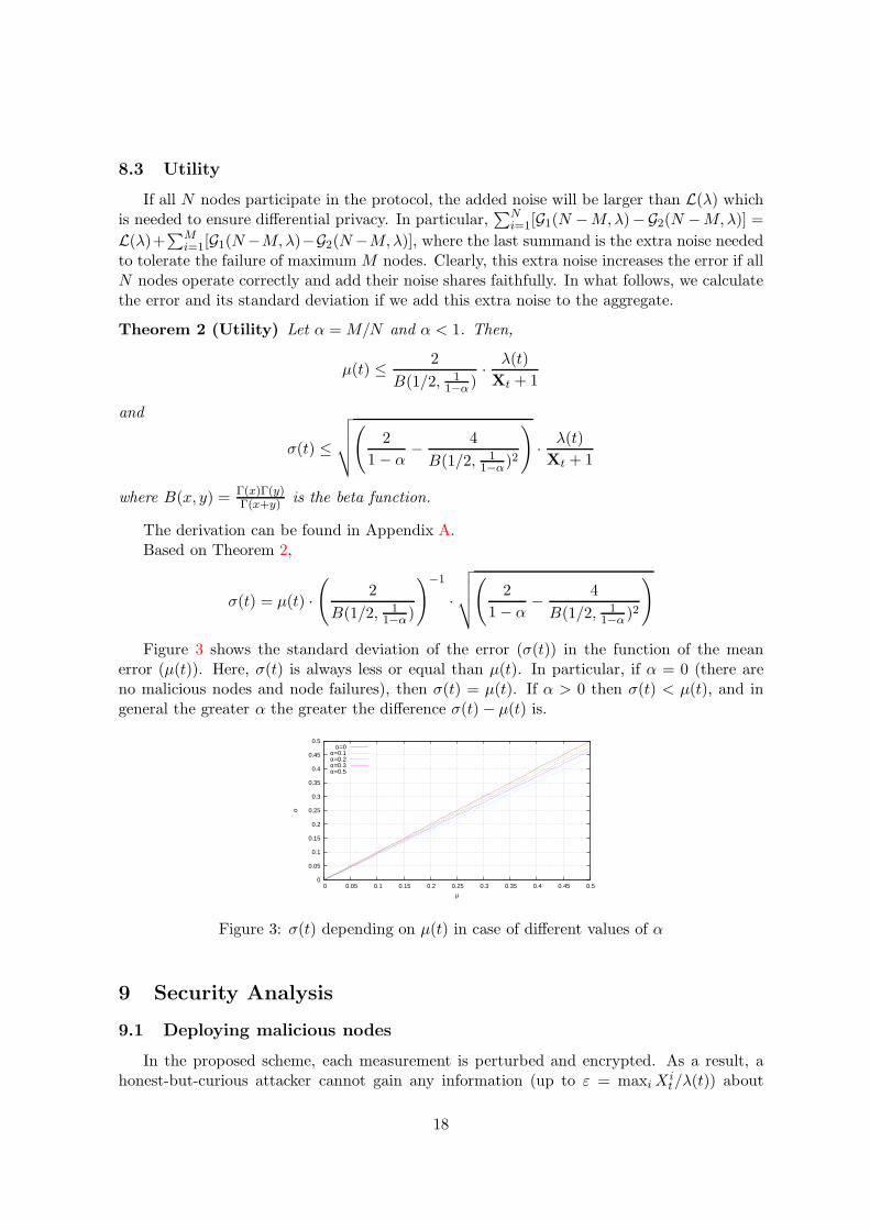
Theorem 2 (Utility) Let α = M/N and α < 1. Then,

µ(t) ≤ 2

B(1/2, 11−α )

· λ(t)

Xt + 1

and

σ(t) ≤

√

√

√

√

(

2

1 − α− 4

B(1/2, 11−α)2

)

· λ(t)

Xt + 1

where B(x, y) = Γ(x)Γ(y)Γ(x+y) is the beta function.

The derivation can be found in Appendix A.Based on Theorem 2,

σ(t) = µ(t) ·(

2

B(1/2, 11−α)

)−1

·

√

√

√

√

(

2

1 − α− 4

B(1/2, 11−α )2

)

Figure 3 shows the standard deviation of the error (σ(t)) in the function of the meanerror (µ(t)). Here, σ(t) is always less or equal than µ(t). In particular, if α = 0 (there areno malicious nodes and node failures), then σ(t) = µ(t). If α > 0 then σ(t) < µ(t), and ingeneral the greater α the greater the difference σ(t) − µ(t) is.

0

0.05

0.1

0.15

0.2

0.25

0.3

0.35

0.4

0.45

0.5

0 0.05 0.1 0.15 0.2 0.25 0.3 0.35 0.4 0.45 0.5

σ

µ

α=0α=0.1α=0.2α=0.3α=0.5

Figure 3: σ(t) depending on µ(t) in case of different values of α

9 Security Analysis

9.1 Deploying malicious nodes

In the proposed scheme, each measurement is perturbed and encrypted. As a result, ahonest-but-curious attacker cannot gain any information (up to ε = maxi X

it/λ(t)) about

18

individual measurements in slot t. This is guaranteed by the encryption scheme and theadded noise.

However, an active attacker, which deploys T malicious nodes, may be able to:

• reduce the noise level by limiting (or omitting) the gamma noise added by maliciousnodes. As a result, the sum of the noise shares will not equal to the laplacian noisewhich can decrease the privacy of users. However, observe that due to the robustnessproperty of our scheme detailed in Section 8 we add extra noise to tolerate M nodefailures. If we increase M with T , then we will add enough extra noise to tolerate thistype of attack.

• decrypt Enc(Xit) of vi and retrieve the perturbed data. As individual data is only

weakly noised, the attacker might infer some information from them, and therefore,compromise privacy. However, as the (homomorphic) encryption scheme that we usedis provably secure [], and nodes are assumed to be tamper-resistant, the only way to dothat is to retrieve the dummy keys of vi. Because the participating nodes are selectedrandomly for each message, this can only be achieved if all participating nodes of vi aremalicious and the supplier is also malicious (i.e., the adversary knows key K ′

i). Thishappens if vi does not select any honest participating node that has a probability of(1 − w

N−1 )N−T−1. Therefore, setting w appropriately is crucial to defend against thistype of attack. For instance, it is easy to check that if N = 100 and 50% of the nodesare malicious (which anyway should be a quite strong assumption), then setting w to30 results in success probability of 1.8 ·10−8. This means that if an epoch is 5 min long,then the adversary will compromise 1 measurement during 458 years in average.

Finally, note also this is the success probability of the adversary in a single slot. Asa result, a supplier that succeeds the previous attack only gets a single (noisy) mea-surement of the customer (corresponding to a single epoch). As a node selects differentparticipating nodes in each slot, the probability that the adversary gets k differentmeasurements of the node is (1 − w

N−1)k(N−T−1), which is even smaller.

9.2 Lying supplier

Lying about non-responding nodes

In addition to deploying malicious (fake) nodes, a malicious supplier can lie about thenon-responding nodes. Indeed, a malicious supplier might pretend that a node vi did notrespond in the first round. As a result, and as described in Section 8.2.2, the participatingnodes of vi will disclose vi’s dummy keys that allows the supplier to decrypt vi’s contribution.However, vi chooses its participating nodes randomly and changes them for each message,and hence, the supplier can only guess them.

In particular, the contribution of vi is secured (i.e., cannot be decrypted), as long as thereis at least one dummy key of vi that is not known to the supplier. More precisely, in orderto recover vi’s measurement, the supplier needs the sum of its random key Ci and its dummykeys. There are three types of vi’s dummy keys: the first is shared with a malicious node, andhence, known to the supplier. The second is asked from vi by the supplier in the second round,and vi replies with the sum of Ci and the asked keys. Finally, the rest is shared with honestparticipating nodes and not asked from vi in the second round. Apparently, if vi has at leastone dummy key from the last group, its measurement cannot be recovered. In particular, if vj

19

is a participating honest node of vi and dkeyi,indi[j] is not asked from vi in the second round,it could be recovered only from vj ’s messages. However, vj sends Cj + dkeyi,indi[j], where Cj

is only known to vj, and thus, the supplier cannot recover dkeyi,indi[j].Nevertheless, it may happen that vi does not have any third-type dummy key (i.e., the

supplier asks for all the dummy keys shared with honest nodes in the second round). Then,the supplier can easily recover vi’s measurement by combining its malicious dummy keys andthe sum of the keys sent by vi to the supplier. However, the supplier can only guess vi’sparticipating nodes7. Assuming that the supplier can ask vi for maximum M dummy keysin the second round, the probability that all participating nodes of vi are either malicious orspecified as non-responding nodes by the supplier is less than (1 − w

N−1 )N−(T+M)−1. Using

α = (T + M)/N and β = w/N , then (1 − wN−1 )N−(T+M)−1 = (1 − β

1−N−1 )N(1−α)−1. Thisprobability is depicted in Figure 4 depending on α, β and N .

1e-10

1e-08

1e-06

0.0001

0.01

1

0 0.2 0.4 0.6 0.8 1

β

α=0α=0.1α=0.3α=0.4α=0.5α=0.6α=0.7α=0.8

(a) N=100

1e-10

1e-08

1e-06

0.0001

0.01

1

0 0.2 0.4 0.6 0.8 1

β

α=0α=0.1α=0.3α=0.4α=0.5α=0.6α=0.7α=0.8

(b) N=300

Figure 4: Success probability of guessing participating nodes depending on β and differentvalues of α and N .

Lying about cluster size

Another strategy for the supplier to compromise the privacy of users is to lie about thecluster size. If the supplier pretends that the cluster size N ′ is larger than it really is (i.e.,N ′ > N), the noise added by each node will be underestimated. In fact, each node willcalibrate its noise based on Formula (1) using N ′ instead of N . As a result, the aggregatednoise at the supplier will be smaller than necessary to guarantee sufficient differential privacy.

In order to prevent this attack, a solution would be to set the cluster size to a fixedvalue. For example, all clusters should have a size of 100. Although simple and efficient, thissolution is not flexible and might not be applicable to all scenarios. Another option is that thesupplier publishes together with the list of cluster nodes, a self-signed certificate (containinga timestamp, the cluster id and the node information) of each node of the cluster. That way,each node could verify the cluster size and get information about its constituting nodes (recallthat the DH certificate of an honest node described in Section 7.1 cannot be forged by thesupplier).

7Note that all nodes send responses in the second round, and the randomness of Ci ensures that the suppliercannot gain any knowledge about the participating nodes of any nodes.

20

10 Simulation results

10.1 Available datasets

Although several research projects were performed in the last two decades aiming tocharacterize the electricity demand model of different households [10], they only providehigh-level statistics: instead of the high resolution demand data, an average consumptionvalue of the given hour of the day is published, where the average is taken on a few weekslong monitoring campaign. This data does not suit our purpose, as we are interested in theconsumption values at finer sampling rates; we need the demand data of each household atevery few minutes (like every 5, 10, 15 min). Intuitively, higher resolution aggregate hashigher variance, and thus, it is much more privacy sensitive. In addition, if, for a given timeslot, we take the average of several measurements taken in the given slot but on differentdays, then we also decrease the variance by “smoothing” out the real time consumption.

10.2 A high-resolution electricity demand model

Due to the lack of high-resolution real world data, we implemented a domestic electricitydemand model [22] that can generate one-minute resolution synthetic consumption data ofdifferent households. This model follows a bottom-up approach and simulates each appliancein a household. The simulator includes 33 different appliances which are randomly assignedto every household based on real deployment statistics. The model also includes a separatelighting model which takes into account the level of natural daylight depending on the monthof the year. The number of residents in each household is randomly selected between 1 and5. A trace is associated to a household and generated as follows: (1) A number of activepersons is selected according to some distribution derived from real statistics. This numbermay vary as some members can enter or leave the house. (2) A set of appliances is thenselected and activated at different time of the day according to an other distribution, whichwas also derived from real statistics.

The input of the simulator is the number of households, the month of the day, and thetype of the day (either a working or weekend day). The output is the power demand model(1-min profile) of all appliances in each household on the given day.

Using this simulator, we generated the 5, 10, and 15-min electricity consumption data of3000 users.

10.3 Adding noise

Each trace was then sanitized according to our scheme. The noise added in each slot(i.e., λ(t)) is set to the maximum consumption in the slot (i.e., λ(t) = max1≤i≤N Xi

t wherethe maximum is taken on all users in the cluster). This amount of noise ensures ε = 1indistinguishability for individual measurements in all slots. Although one can increase λ(t)to get better privacy, the error will also increase. Note that the error µε′(t) for other ε′ 6= εvalues if µε(t) is given is µε′(t) = ε

ε′ ·µε(t). We assume that λ(t) = maxi Xit is known a priori.

10.4 Error and the cluster size

We are interested in the dependence of the error (µ(t)) on the cluster size (N). Recallthat higher N results in higher Xt which decreases µ(t) in Definition 2.

21

10.4.1 Random clustering

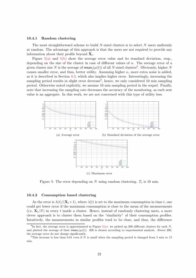
The most straightforward scheme to build N -sized clusters is to select N users uniformlyat random. The advantage of this approach is that the users are not required to provide anyinformation about their profile beyond Xt.

Figure 5(a) and 5(b) show the average error value and its standard deviation, resp.,depending on the size of the cluster in case of different values of α. The average error of agiven cluster size N is the average of meant(µ(t)) of all N -sized clusters8. Obviously, higher Ncauses smaller error, and thus, better utility. Assuming higher α, more extra noise is added,as it is described in Section 8.3, which also implies higher error. Interestingly, increasing thesampling period results in slight error decrease9, hence, we only considered 10 min samplingperiod. Otherwise noted explicitly, we assume 10 min sampling period in the sequel. Finally,note that increasing the sampling rate decreases the accuracy of the monitoring, as each sentvalue is an aggregate. In this work, we are not concerned with this type of utility loss.

0.01

0.02 0.03 0.04

0.07 0.1

0.15 0.2 0.3

0.5

1

0 100 200 300 400 500 600 700 800 900 1000

N

α=0α=0.1α=0.2α=0.3α=0.5

(a) Average error

0.01

0.02 0.03 0.04

0.07 0.1

0.15 0.2 0.3

0.5

1

0 100 200 300 400 500 600 700 800 900 1000

N

α=0α=0.1α=0.2α=0.3α=0.5

(b) Standard deviation of the average error

0.01

0.02 0.03 0.04

0.07 0.1

0.15 0.2 0.3

0.5

1

0 100 200 300 400 500 600 700 800 900 1000

N

α=0α=0.1α=0.2α=0.3α=0.5

(c) Maximum error

Figure 5: The error depending on N using random clustering. Ts is 10 min.

10.4.2 Consumption based clustering

As the error is λ(t)/(Xt +1), where λ(t) is set to the maximum consumption in time t, onecould get lower error if the maximum consumption is close to the mean of the measurements(i.e, Xt/N) in every t inside a cluster. Hence, instead of randomly clustering users, a moreclever approach is to cluster them based on the “similarity” of their consumption profiles.Intuitively, the measurements in similar profiles tend to be close, and thus, the difference

8In fact, the average error is approximated in Figure 5(a): we picked up 200 different clusters for each N ,and plotted the average of their meant(µ(t)). 200 is chosen according to experimental analysis. Above 200,the average error do not change significantly.

9This increase is less than 0.01 even if N is small when the sampling period is changed from 5 min to 15min.

22

between the maximum consumption and Xt/N should also be smaller than in a randomcluster.

Although there are multiple distance metrics to measure profile similarity, we just comparethem based on the average daily consumption. In contrast to random clustering, this requiresusers to share their daily averages which may leak some information about their profile beyondXt. However, the supplier does not need to know the high resolution profiles to calculate thedaily averages; it can be derived from the (monthly) aggregate consumption of each user,which is though generally revealed for billing.

The N -sized clusters are created by calculating daily consumption levels such that thenumber of users whose daily average falls into the same level is exactly N . Then, all usersform a cluster who are in the same level. This can be implemented by simply sorting the3000 users according to their daily averages where each consecutive N users forms a cluster.If the size of the last sequence is less than N , we omit the corresponding users from furthercalculations.

Figure 6(a) and 6(b) show the average error and its deviation, resp., calculated identicallyto random clustering. Comparing Figure 6 and 5, consumption based clustering has lowererror with 0.01-0.05 than the random one depending on N . For instance, while randomclustering provides an average error of 0.13 with N = 100 users in a cluster, consumptionbased clustering has 0.07. The difference decreases as N increases. There are more significantdifferences between the standard deviations and the worst cases: on lower value of N , thestandard deviation of the average error in random clustering is almost twice as large as inconsumption based clustering (Figure 6(b) and 5(b)). To compute the worst case error, ata given N , the maximum error is computed in all slots, which is the highest cluster errorthat can occur in a slot with cluster size N . Then, the average of these maximum errors (theaverage is taken on all slots) are plotted in Figure 5(c) and 6(c). Apparently, the worst caseerror in random clustering is much higher than in consumption based clustering, as randomclustering may put high and low consuming user into the same cluster.

0.01

0.02 0.03 0.04

0.07 0.1

0.15 0.2 0.3

0.5

1

0 100 200 300 400 500 600 700 800 900 1000

N

α=0α=0.1α=0.2α=0.3α=0.5

(a) Average error

0.01

0.02 0.03 0.04

0.07 0.1

0.15 0.2 0.3

0.5

1

0 100 200 300 400 500 600 700 800 900 1000

N

α=0α=0.1α=0.2α=0.3α=0.5

(b) Standard deviation of the average error

0.01

0.02 0.03 0.04

0.07 0.1

0.15 0.2 0.3

0.5

1

0 100 200 300 400 500 600 700 800 900 1000

N

α=0α=0.1α=0.2α=0.3α=0.5

(c) Maximum error

Figure 6: The error depending on N using consumption based clustering. Ts is 10 min.

23

10.5 Boosting utility by lowering noise

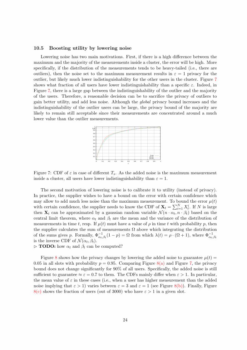
Lowering noise has two main motivations. First, if there is a high difference between themaximum and the majority of the measurements inside a cluster, the error will be high. Morespecifically, if the distribution of the measurements tends to be heavy-tailed (i.e., there areoutliers), then the noise set to the maximum measurement results in ε = 1 privacy for theoutlier, but likely much lower indistinguishability for the other users in the cluster. Figure 7shows what fraction of all users have lower indistinguishability than a specific ε. Indeed, inFigure 7, there is a large gap between the indistinguishability of the outlier and the majorityof the users. Therefore, a reasonable decision can be to sacrifice the privacy of outliers togain better utility, and add less noise. Although the global privacy bound increases and theindistinguishability of the outlier users can be large, the privacy bound of the majority arelikely to remain still acceptable since their measurements are concentrated around a muchlower value than the outlier measurements.

0.1

0.2

0.3

0.4

0.5

0.6

0.7

0.8

0.9 0.95

1

0 0.1 0.2 0.3 0.4 0.5 0.6 0.7 0.8 0.9 1

ε

5 min10 min15 min

Figure 7: CDF of ε in case of different Ts. As the added noise is the maximum measurementinside a cluster, all users have lower indistinguishability than ε = 1.

The second motivation of lowering noise is to calibrate it to utility (instead of privacy).In practice, the supplier wishes to have a bound on the error with certain confidence whichmay allow to add much less noise than the maximum measurement. To bound the error µ(t)with certain confidence, the supplier needs to know the CDF of Xt =

∑Ni=1 Xi

t . If N is largethen Xt can be approximated by a gaussian random variable N (n · αt, n · βt) based on thecentral limit theorem, where αt and βt are the mean and the variance of the distribution ofmeasurements in time t, resp. If µ(t) must have a value of ρ in time t with probability p, thenthe supplier calculates the sum of measurements Ω above which integrating the distributionof the sums gives p. Formally, Φ−1

αt,βt(1 − p) = Ω from which λ(t) = ρ · (Ω + 1), where Φ−1

αt,βt

is the inverse CDF of N (αt, βt).⊲ TODO: how αt and βt can be computed?

Figure 8 shows how the privacy changes by lowering the added noise to guarantee µ(t) =0.05 in all slots with probability p = 0.95. Comparing Figure 8(a) and Figure 7, the privacybound does not change significantly for 90% of all users. Specifically, the added noise is stillsufficient to guarantee ≈ ε = 0.7 to them. The CDFs mainly differ when ε > 1. In particular,the mean value of ε in these cases (i.e., when a user has higher measurement than the addednoise implying that ε > 1) varies between ε = 3 and ε = 1 (see Figure 8(b)). Finally, Figure8(c) shows the fraction of users (out of 3000) who have ε > 1 in a given slot.

24

0.1

0.2

0.3

0.4

0.5

0.6

0.7

0.8

0.9 0.95

1

0 0.1 0.2 0.3 0.4 0.5 0.6 0.7 0.8 0.9 1

ε

(a) CDF of ε when ε < 1.

2

4

6

8

10

12

14

00:00 02:00 04:00 06:00 08:00 10:00 12:00 14:00 16:00 18:00 20:00 22:00 00:00

Time

maxmean

95% conf.

(b) Statistics of ε when when ε > 1.

0

0.01

0.02

0.03

0.04

0.05

0.06

0.07

0.08

0.09

00:00 02:00 04:00 06:00 08:00 10:00 12:00 14:00 16:00 18:00 20:00 22:00 00:00

Time

(c) Fraction of users who has ε > 1.

Figure 8: Lowering added noise to guarantee µ(t) = 0.05 in all t with probability 0.95. Ts is10 min.

10.6 Privacy over multiple slots

So far, we have considered the privacy of individual slots and added noise to guaranteeε = 1 privacy in each slot. However, the output are multiple aggregates as we release oneaggregate per slot. For instance, if one watches TV along multiple slots, we have guaranteedthat the adversary cannot tell if the TV is watched in any single slot (up to ε = 1), but it maybe able to tell that the TV is watched in a given time period having s slots (s > 1) (the privacybound of this is εs = ε · s due to the composition property of differential privacy). Based onTheorem 1, we need to add noise λ(t) =

∑si=1 maxi X

it to each aggregate to guarantee εs = 1

bound in consecutive s slots, which results in much higher error than in the case of s = 1that we have assumed so far.

Obviously, using the LPA technique, we cannot guarantee reasonably low error if s in-creases, as the necessary noise λ(t) =

∑si=1 maxi X

it can be large. In order to keep the error

λ(t)/∑N

i=1 Xit low while ensuring better privacy than s · ε, one can increase the number of

users inside each cluster (i.e., N). In the sequel, we investigate what privacy we can guaranteeto some activities by adding the noise described in Section 10.3.

To illustrate the calculation of the bound εs with a given noise λ(t) when s > 1, considerFigure 9. The consumption of a user i (i.e., Xi

t) and the added noise λ(t) is plotted inFigure 9(a). Suppose we want to know what privacy user i has between 14:00 and 18:00.The bound ε(t) = Xi

t/λ(t) in a single slot t is plotted in Figure 9(b). The bound εs forthe s = 24 slots between 14:00 (84th slot) and 18:00 (108th slot) is

∑108t=84 ε(t) based on the

composition property of differential privacy, which is 7.52 in the current example. In general,εs(t) =

∑t+si=t ε(i).

Figure 10 shows what privacy a user has in average in our dataset depending on the clustersize in case of different values of s. For a given N and s, we computed maxt εs(t) for all users.The average of all these maximum bounds are plotted.

As the cluster size increases, the bound becomes smaller. This is because the cluster

25

0

200

400

600

800

1000

1200

1400

1600

1800

00:00 02:00 04:00 06:00 08:00 10:00 12:00 14:00 16:00 18:00 20:00 22:00 00:00

Energ

y (W

h)

Time

λ(t)consumption

s=24 slots

(a) Consumption and the added noise λ(t)

0

0.1

0.2

0.3

0.4

0.5

0.6

0.7

0.8

0.9

1

00:00 02:00 04:00 06:00 08:00 10:00 12:00 14:00 16:00 18:00 20:00 22:00 00:00

ε

Time

ε(t)

s = 24 slots

(b) ε(t) is the bound in slot t. The bound εs

between 14:00 and 18:00 is the shaded regionbelow the curve of ε(t).

Figure 9: Privacy in a given time window.

will have more users, and the maximum consumption (i.e., the noise) inside a cluster alsoincreases (recall that increasing N in consumption based clustering increases the averageconsumption level of each cluster). Also note that increasing the sampling period alsoincreases privacy.⊲ TODO: why?

2

3

4

5 6 7

10

15

20

30

0 100 200 300 400 500 600 700 800 900 1000

N

15 min30 min

1 h4 h8 h

1 day

(a) Ts is 5 min

1

2

3

4 5 6 7

10

15

20

30

0 100 200 300 400 500 600 700 800 900 1000

N

10 min30 min

1 h4 h8 h

1 day

(b) Ts is 10 min

1

2

3

4

5 6 7

10

15

20

0 100 200 300 400 500 600 700 800 900 1000

N

15 min30 min

1 h4 h8 h

1 day

(c) Ts is 15 min

Figure 10: Privacy of all appliances in s long time windows (where s is 10 min, 15 min, 30min, 1 h, 4 h, 8 h, 1 day) using different sampling periods.

10.6.1 Privacy of appliances

We interpret the privacy of different activities (such as watching TV or cooking) betweentime t1 and t2 analogously to the example illustrated before. The only difference is that theconsumption represents the sum consumption of the appliances (instead of the consumptionof all appliances in Figure 9(a)) which are used to perform the activity. For instance, if

26

we are interested in what privacy the user had when he watched a game in the TV lastnight between 18:00 and 20:00 by adding noise λ(t), we need to calculate

∑120t=108 ε(t), where

ε(t) = TV’s consumption in t/λ(t).Table 1 in Appendix B summarizes the average bound (computed identically as in Figure

10) of the main appliances used in our simulator. In addition, the table contains the standarddeviation of maxt εs(t) and its maximum value in the whole dataset. The appliances aredivided into two major groups: the usage of active appliances indicate that the user is athome and uses the appliance (their consumption significantly changes during their activeusage such as iron, vacuum, kettle, etc.), whereas passive appliances have more or less identicalconsumption regardless the user is at home (like fridge, freezers, storage heater, etc.)10. Ingeneral, appliances having lower consumption threats privacy less than devices with higherenergy demands. Obviously, εs increases when s increases since an appliance is used morefrequently within longer periods.

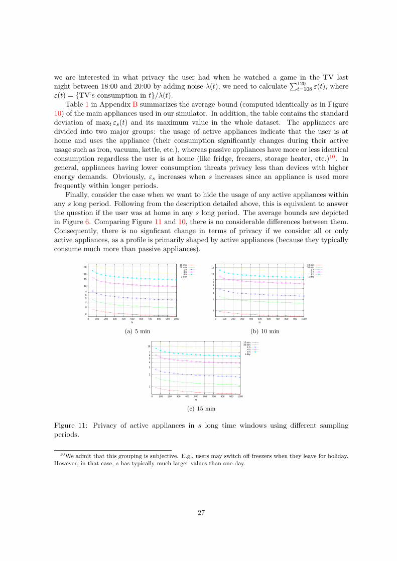
Finally, consider the case when we want to hide the usage of any active appliances withinany s long period. Following from the description detailed above, this is equivalent to answerthe question if the user was at home in any s long period. The average bounds are depictedin Figure 6. Comparing Figure 11 and 10, there is no considerable differences between them.Consequently, there is no signficant change in terms of privacy if we consider all or onlyactive appliances, as a profile is primarily shaped by active appliances (because they typicallyconsume much more than passive appliances).

2

3

4

5 6 7

10

15

20

30

0 100 200 300 400 500 600 700 800 900 1000

N

15 min30 min

1 h4 h8 h

1 day

(a) 5 min

1

2

3

4

5 6 7

10

15

0 100 200 300 400 500 600 700 800 900 1000

N

10 min30 min

1 h4 h8 h

1 day

(b) 10 min

1

2

3

4

5 6 7

10

0 100 200 300 400 500 600 700 800 900 1000

N

15 min30 min

1 h4 h8 h

1 day

(c) 15 min

Figure 11: Privacy of active appliances in s long time windows using different samplingperiods.

10We admit that this grouping is subjective. E.g., users may switch off freezers when they leave for holiday.However, in that case, s has typically much larger values than one day.

27

11 Conclusion and Future work

References

[1] R. Anderson and S. Fuloria. On the security economics of electricity metering. InProceedings of the Ninth Workshop on the Economics of Information Security (WEIS2010), June 2010.

[2] R. Anderson and S. Fuloria. Who controls the off switch? In Proceedings of the IEEESmartGridComm, June 2010.

[3] J.-M. Bohli, C. Sorge, and O. Ugus. A privacy model for smart metering. In Proceedingsof the IEEE International Conference on Communications (ICC 2010), 2010.

[4] C. Castelluccia, E. Mykletun, and G. Tsudik. Efficient aggregation of encrypted datain wireless sensor networks. In ACM/IEEE Mobiquitous Conference, San Diego, USA,July 2005.

[5] R. Cramer, I. Damgard, and J. B. Nielsen. Multiparty computation from thresholdhomomorphic encryption. In EUROCRYPT, 2001.

[6] W. Diffie and M. Hellman. New directions in cryptography. IEEE Transactions onInformation Theory, 22:644–654, 1976.

[7] C. Dwork, K. Kenthapadi, F. McSherry, I. Mironov, and M. Naor. Our data, ourselves:Privacy via distributed noise generation. In Proceedings of EUROCRYPT, 2006.

[8] C. Dwork, F. McSherry, K. Nissim, and A. Smith. Calibrating noise to sensitivity inprivate data analysis. In Proceedings of the 3rd IACR Theory of Cryptography Conference,2006.

[9] C. Efthymiou and G. Kalogridis. Smart grid privacy via anonymization of smart meteringdata. In Proceedings of IEEE SmartGridComm, October 2010.

[10] EIE/05/124/SI2.419657. Residential monitoring to decrease energy use and carbon emis-sions in europe (remodece). In http://remodece.isr.uc.pt/, 2008.

[11] P. A. Fouque, G. Poupard, and J. Stern. Sharing decryption in the context of voting orlotteries. In Proceedings of the 4th International Conference on Financial Cryptography(FC’00), pages 90–104, 2001.

[12] F. D. Garcia and B. Jacobs. Privacy-friendly energy-metering via homomorphic encryp-tion. In Proceedings of the 6th Workshop on Security and Trust Management (STM2010), 2010.

[13] O. Goldreich. http:/www.wisdom.weizmann.ac.il/oded/PS/prot.ps.

[14] G. Hart. Nonintrusive appliance load monitoring. Proceedings of the IEEE, 80(12):1870–1891, December 1992.

28

[15] G. Kalogridis, C. Efthymiou, S. Denic, T. A. Lewis, and R. Cepeda. Privacy for smart me-ters: Towards undetectable appliance load signatures. In Proceedings of the First IEEEInternational Conference on Smart Grid Communications (SmartGridComm 2010), Oc-tober 2010.

[16] A. Korolova, K. Kenthapadi, N. Mishra, and A. Ntoulas. Releasing search queries andclicks privately. In Proceedings of WWW 2009, 2009.

[17] S. Kotz, T. J. Kozubowski, and K. Podgorski. The Laplace distribution and general-izations: a revisit with applications to Communications, Economics, Engineering, andFinance. Birkhauser, 2001.

[18] H. Lam, G. Fung, and W. K. Lee. A novel method to construct taxonomy electri-cal appliances based on load signatures. IEEE Transactions on Consumer Electronics,53(2):653–660, December 2007.

[19] A. Molina-Markham, P. Shenoy, K. Fu, E. Cecchet, and D. Irwin. Private memoirs of asmart meter. In Proceedings of the 2nd ACM Workshop on Embedded Sensing Systemsfor Energy-Efficiency in Building (Buildsys 2010), 2010.

[20] V. Rastogi and S. Nath. Differentially private aggregation of distributed time-series withtransformation and encryption. In Proceedings of the ACM SIGMOD/PODS Conference(SIGMOD 2010), June 2010.

[21] A. Rial and G. Danezis. Privacy-preserving smart metering. In Technical Report, MSR-TR-2010-150. Microsoft Research, 2010.

[22] I. Richardson, M. Thomson, D. Infield, and C. Clifford. Domestic electricity use: Ahigh-resolution energy demand model. Energy and Buildings, 42:1878–1887, 2010.

[23] E. Shi, T. Chan, E. Rieffel, R. Chow, and D. Song. Privacy-preserving aggregation oftime-series data. In Network and Distributed System Security Symposium (NDSS). Toappear., 2011.

29

A Proof of Theorem 2 (Utility)

Lemma 2 (Integral property of the Bessel function [17]) Let

Kϑ(x) =1

2

(x

2

)ϑ∫ ∞

0t−ϑ−1 exp

(

−t − x2

4t

)

dt, x > 0

define the modified Bessel function of the third kind with index ϑ ∈ R. For any γ > 0 andγ, ν such that γ + 1 ± ν > 0

∫ ∞

0xγKν(ax)dx =

2γ−1

aγ+1Γ

(

1 + γ + ν

2

)

Γ

(

1 + γ − ν

2

)

Lemma 3 Let G1,G2 be i.i.d gamma random variables with parameters (n, λ). Then,

E|G1(n, λ) − G2(n, λ)| =2λ

B(

12 , 1

n

) (2)

and

Var |G1(n, λ) − G2(n, λ)| =

(

2

n− 4

B(

12 , 1

n

)2

)

λ2 (3)

where B(x, y) is the beta function defined as B(x, y) = Γ(x)Γ(y)Γ(x+y) .

Proof (of Lemma 3) Consider Y = G1 − G2. The characteristic function of Y is

φY(t) =

(

1

1 + iλt

)1n

·(

1

1 − iλt

)1n

=

(

1

1 + λ2t2

)1n

which is a special case of the characteristic function of the Generalized Asymetric Laplacedistribution (GAL) with parameters (θ, κ, ω, τ):

φGAL(t) = eiθt

(

1

1 + i√

22 ωκt

)τ

·(

1

1 − i√

22κ ωt

)τ

where θ = 0, κ = 1, ω =√

2λ, and τ = 1/n. The density function of GAL(θ, κ, ω, τ) whenθ = 0 and κ = 1 is

fGAL(x) =

√2

ωτ+1/2Γ(τ)√

π

( |x|√2

)τ−1/2

Kτ−1/2(√

2|x|/ω)

where Kτ−1/2(√

2ω |x|) is the Bessel function defined in Lemma 2. In addition,

E|Y| =

∫ ∞

−∞|x|fGAL(x)dx = 2 ·

∫ ∞

0x

√2

ωτ+1/2Γ(τ)√

π

(

x√2

)τ−1/2

Kτ−1/2(√

2x/ω)dx

which follows from the symmetry property of fGAL(x) (φY(t) is is real valued). After refor-mulation, we have

E|Y| =2√

2√

2τ−1/2

ωτ+1/2Γ(τ)√

π

∫ ∞

0xτ+1/2Kτ−1/2(

√2x/ω)dx

30

Now, we can apply Lemma 2 for the integral and we obtain

E|Y| =√

2 · w · Γ(τ + 12)

Γ(12)√

π

after simple derivation. Using that√

π = Γ(1/2) and B(x, y) = Γ(x)(y)Γ(x+y) , we have

E|Y| =

√2

B(1/2, τ)· w

Applying ω =√

2λ and τ = 1/n, we arrive at Equation (2).To prove Equation (3), consider that

Var(|Y|) = E|Y|2 − [E|Y|]2

whereE|Y|2 = E(Y2) = E(G2

1) + E(G22) − 2 · E(G1) · E(G2)

Using that E(G21) = E(G2

2) = (1/n2 + 1/n)λ2, we obtain Equation (3).

Now, we can easily prove Theorem 2.

Proof (of Theorem 2)

E|N∑

i=1

(Xit − Xi

t)| =

= E|N∑

i=1

G1(N − M,λ) −N∑

i=1

G2(N − M,λ)| =

(using that∑n

i=1 G(ki, λ) = G(1/∑n

i=11ki

, λ))

= E|G1(1 − M/N,λ) − G2(1 − M/N,λ)| =

(using α = M/N and applying Lemma 3)

=2

B(1/2, 11−α )

λ

The standard deviation√

Var |∑Ni=1(X

it − Xi

t)| can be derived identically.

B Privacy of some ordinary appliances

31

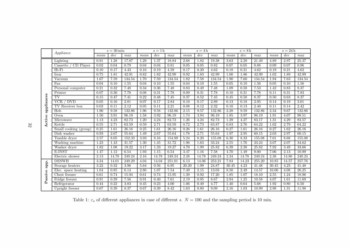
Appliances = 30min s = 1h s = 4 h s = 8h s = 24 h

mean dev max mean dev max mean dev max mean dev max mean dev max

Activ

eappliances

Lighting 0.91 1.28 17.87 1.29 1.37 18.84 2.68 1.82 19.38 3.63 2.29 21.49 4.89 2.97 25.37Cassette / CD Player 0.02 0.04 0.79 0.04 0.04 0.81 0.05 0.05 0.82 0.07 0.05 0.88 0.09 0.07 0.96Hi-Fi 0.10 0.17 4.43 0.16 0.19 4.59 0.17 0.20 4.62 0.18 0.21 4.62 0.19 0.21 4.62Iron 0.75 1.81 42.91 0.82 1.82 42.99 0.92 1.83 42.99 1.00 1.86 42.99 1.02 1.89 42.99Vacuum 1.67 7.59 134.54 1.70 7.59 134.54 1.82 7.58 134.54 1.90 7.60 134.54 1.94 7.63 134.54Fax 0.04 0.10 1.55 0.04 0.10 1.55 0.04 0.10 1.55 0.05 0.10 1.56 0.05 0.10 1.56Personal computer 0.21 0.32 7.48 0.34 0.36 7.48 0.83 0.49 7.48 1.09 0.58 7.53 1.42 0.83 8.37Printer 0.07 0.30 7.78 0.08 0.31 7.78 0.09 0.31 7.78 0.10 0.31 7.78 0.11 0.31 7.83TV 0.15 0.47 7.41 0.22 0.48 7.45 0.37 0.52 7.45 0.45 0.58 8.37 0.50 0.63 8.37VCR / DVD 0.05 0.16 2.81 0.07 0.17 2.84 0.10 0.17 2.89 0.13 0.18 2.95 0.14 0.19 3.01TV Receiver box 0.03 0.11 2.12 0.05 0.11 2.21 0.08 0.12 2.32 0.10 0.13 2.40 0.11 0.14 2.42Hob 1.90 9.58 132.86 1.96 9.58 132.86 2.15 9.57 132.86 2.28 9.59 132.86 2.34 9.67 132.86Oven 1.50 3.91 96.19 1.58 3.92 96.19 1.74 3.94 96.19 1.85 3.97 96.19 1.91 4.07 98.51Microwave 1.13 4.23 82.73 1.20 4.24 82.73 1.26 4.24 82.73 1.29 4.27 83.17 1.31 4.29 83.57Kettle 0.55 2.71 63.59 0.59 2.71 63.59 0.72 2.73 63.87 0.83 2.76 64.22 1.02 2.79 64.22Small cooking (group) 0.25 1.61 26.16 0.25 1.61 26.16 0.26 1.61 26.16 0.27 1.61 26.16 0.27 1.62 26.16Dish washer 0.93 2.67 55.64 1.49 2.67 55.64 1.78 2.71 55.64 1.97 2.95 60.15 2.03 2.97 60.15Tumble dryer 2.57 8.05 152.33 3.93 8.16 154.99 5.24 8.20 155.08 6.30 8.33 155.08 7.01 8.68 155.08Washing machine 1.23 1.43 31.57 1.30 1.45 31.72 1.96 1.63 33.24 2.55 1.76 33.24 3.07 2.07 34.62Washer dryer 1.82 1.08 19.22 3.17 1.33 19.27 4.70 1.99 25.82 6.39 2.38 25.82 7.92 3.49 33.66E-INST 1.47 1.12 6.54 1.93 1.15 6.54 3.47 1.16 7.58 4.70 1.49 9.00 7.06 2.13 10.99Electric shower 2.13 14.78 249.24 2.16 14.78 249.24 2.28 14.78 249.24 2.34 14.78 249.24 2.38 14.80 249.24

Passiv

eapp. DESWH 3.34 14.01 249.29 4.04 14.04 251.01 6.13 14.06 253.21 7.83 14.23 255.20 10.85 14.57 257.76

Storage heaters 3.22 0.32 3.96 5.64 0.56 6.95 20.20 1.99 24.87 30.45 4.23 41.48 30.45 4.23 41.48Elec. space heating 1.64 0.85 6.14 2.86 1.07 7.54 7.49 2.15 13.03 8.50 2.49 14.57 10.06 4.08 26.25Chest freezer 0.61 0.74 15.94 0.61 0.74 15.95 1.39 0.92 17.20 1.85 1.07 18.10 2.55 1.24 18.96Fridge freezer 0.91 0.39 7.56 0.91 0.40 7.61 2.19 0.95 8.67 2.94 1.25 10.58 4.07 1.61 11.69Refrigerator 0.44 0.22 3.83 0.45 0.23 4.00 1.06 0.49 4.77 1.40 0.64 5.68 1.92 0.80 6.50Upright freezer 0.67 0.39 8.37 0.67 0.39 8.42 1.63 0.80 9.09 2.16 1.03 10.99 2.98 1.31 11.98

Table 1: εs of different appliances in case of different s. N = 100 and the sampling period is 10 min.

32