UJ

I AD-AOI9 325

DIFFERENTIAL GAME GUIDANCE VERSUS PROPORTIONALNAVIGATION FOR AN AIR-TO-AIR MISSILE

SRobin A. Poulter

SAir Force Institute of TechnologyWright-Patterson Air Force Base, Ohio

•: December 1975

DISTRIBUTED BY:

Naltional Technical Information ServiceU. S. DEPARTMENT OF COMMERCE

p"' '"h -- II I II

I . . ...x

DIFFERENTIAL GAMlE 'GUIDANCE VERSUSPROPORTIONAL NAVIGATION FOR AN .. •

AIR-TO-AIR MISSILE '.

Thesis

U-/ GMbC/75-5 Robin A. Poulter

F 1t . Lt. RAF

Approved for public release; distribution unlimited.

$eCCITY CL JISIFCATiON OF YHIS PAGEZ(I 'Whv. Ecau ~ ~tirre_______________ READ IiXSTRU(CTIQNS

" REPORT DOCUMENTATION PAGE SEOR COID M-TIU•NG F(-1.REPORY NUM~BER 2- GOVT A -CESSICN N?. 3. ReECIPIENTS ATALG dMIE

G.A/MC/TS- 5 I4. TITLE (en Su•d•tlre) I, TYPE OF REORI ftiob COVE£el

DIFFERENTIAL GAME GUIDANCE VERSUS AFIT ThesisPROPORTIONAL NAVIGATION FOR AN A. PERFORMING QRQ. REPORT NUMBER

AIR TC-AIR MISSILE7. AUT4-oR(f) S. CONTRACT OR GRANT NUMBER(*)

Robin A. PoulterFlt. Lt RAF

9. PERFORMING ORGANIZATION NAME AND ADDRESS 10. PROGRAM ELEMENT. PROJECT, TASIKAREA A WORK UNIT NUMBE.RS

Air Force Institute of Technology (AU)Wright-Patterson AFB, OH 45433

II. ccmTROLLING OFFICE NAME AND ADDRESS t2. REPORT CATE

December 19751L. NUMBER OFC PAGES

14. MONITORING AGENCY NAML & AODRESSýJfdillfrmt tir ContrJllJnl Office) IS, SECURITY CLASS. (Cf thl rePort)

75.•. DECLASSiFICATION, DOWNGRADINGSCHEOULC•.

16. DISTRIBUTIOt. STATEMENT (of ;hi Report)

Approved for public release; distribut.ion unlimited.

I17. DISTRIBUTION STATEMENT (of the absttrae enitered In Block 20, if different from Repotl)

18. SUPPLEMENTARY NOTES

Approved for public release; lAW AFR O- •i.

S USAFDktector of Information

19. KEY WORDS (Con:lnu. on revere side if neeemry and Identify by block nw.mbwr)

Game TheoryDifferential GamesAir-to-Air MissilesMissile Control

20.ABSTRACT (Cont~nu* an * reverse aide if n#;:**@oyy and identify by block number)

Proportional navigation is a closed loop optimal control for

intercept problem and a quadratic cost function. PRef 6).This paper presents a differential game model of the inter-

cept problem using nonlinear realistic dynamics, free final timeand a terminal cost function related to probability of kill.

With this model proportional navigation is no longer optimal and

DD JAN73 1473 ' UnclassifiedSECURITY CLASSIFICATION OF THIS PAGE (Wh, Dar& E'C!r,*j

ZUncassi fi ed

1K ~~~K ~SrcLJRIY rLASsf P ICA~l' 7 1rý n r~ T A~d~e It :-s,!

t he extent of its nonoptimality is indicated for a range of

saddle point solutions.

A guidance concept based on differential gamne theory isd CeusSed anid is compared to proportional navigation in an off

Tine simulation. The considerable gains made by this scheme iverjproportional navigation provide the incentive to develup a realtime version.

II

I P UnclassifiedSCUiRITY CLASSIFICATION OF THIS PAGE(Wi'hen •C•. EnI-vd)

DIFFERENT!AL GAME GUIDANCE VERSUS PROPORTIONAL

NAVIGATEO% FOR AN AIR-TO-AIR MISSILE

THESIS

Presented to the Faculty of the School of Engineering

of the Air Force institute of Technology

Air University

in Partial Fulfillment of the

Requirements tor the Degree of

Master of Science

by

Robin A. Pouiter, B.Sc.(Hons)

Flight Lieutenant Royal Air Force

Graduate Astronautical Engineering

1 December 1975

Approved for public release; distribution unlimited.

4

L .....

Preface

Differential game models of realistic problems rarely

lead to closed loop laws. Major G. M. Anderson of the

Department of Mechanics has proposed a means of approxi-

mating the closed loop ,la based on updating the open loop

law. This thesis is a result of my work investigating the

applicability of his method to the air-to-air missile

intercept problem using nonlinear dynamics.

I wish to acknowledge the assistance of Major Anderson

both in the work on this thesis and in his sequences on

Optimal Control. I would also like to thank Squadron Leader

F. 0. Reddyhof for his assistance with the missile model

and the proportional navigation scheme.

Lastly, I wish to acknowledge the support of my family

throughout my trials and tribulations.

Robin A. Poulter

I;

WFContents~

Preface . . . . . . . . . . . . . . . . . . . . .

List of Figures ...........................

List of Tables . . . . . . . . . . . . . . . . . vii

Abstract ............... viii

I. Introduction . . . . . . . . . . . . . . . I

Background .......... 3Statement of the Problem .... ... ........ 3Summary ........... . ... ................ 4

II. Differential Game Theory ... ......... .

Pronlem FormulaLion. ........... .Pseudo Closed, Loop Scheae . ....... 9

III Intercept Problem ............ 11

Gam2 Scenario ......... ............. I..j Aircraft Modei . .... ... ............. ii

Missile Model ....... ............. 13Cost '.unction ... .. ............. 13Differential Game Guidance ......... isOptimal Controls ...... ............ 19

tN Proportional Navigation Scheme .... ..... 24

IV. Results ... .. .. .. ................... 2

TPBVP Solution Method ... ......... 27Saddle Point Solutions . . . . . 27Open Loop Controls .......... ........... 29Proportional Navigation Versus Cptimay1Control . . . . . . . . . 32Tuned Proportional Navigation . .. .. 33

Pseudo Closed Loop Guidance .. .. . . 34Open LooU Optimal Evasion .. ....... 36Updated Optimal Evader ... ......... 36Undated Pursuer ............. 38Proportional Navigation with Nonopti'aaiEvasion ................. 39Summary . . . .............. 4

V. Conclusions and Recommendations ...... 42

Conclusions .............. 42Recommendations .... ............ 43

-• •• • .' •• ~ ---- -o--__-_ - _ _~• :

- o•ibliography .... . .................... 44

Appendix A: Tables and Figures .. .. . .. . 45

Appendix B: Nvrnericai Aspects . 94

Vita . . . . . . . . . . . . . . . . . . . . . . . 101

if

Iiv

List of Figures

rigure Pg

1 Line of Sight Angles ... .......... .. 25

2 Optimal Evasion - Optimal Pursuit .... 46

3 Optimal Versus Proportional NavigationBank Angle ....... ............... .. 47

4 Optimal Evasion - Optimal Pursuit . . . . 48

5 Optimal Versus Proportional NavigationBank Angle ....... ............... .. 49

6 Optimal Evasion - Optimal Pursuit . . . 50

7 Optimal Versus Proportional NavigationBank Angle ..... ............ .1....Si

8 Optimal Evasion - Optimal Pursuit . . . . 52

9 Optimal Versus Proportional NavigationBank Angle ................ ............. 53

10 Optimal Evasion - Optimal Pursuit . . . . 54

11 Optimal Versus Proportional NavigationBank Angle ....... ............... .. 55

12 Optimal Evasion - Optimal Pursuit . . . . 56

13 Optimal Evasion - Optimal Pursuit . . . . 57

14 Optimal Evasion - Optimal Pursuit . . . . 58

15 Optimal Versus Proportional NavigationBank Angle ....... ............... .. 59

16 Optimal Evasion - Optimal Pursuit .... 61

17 Optimal Evasion - Proportional NavigationPursuit ........ ................. .. 62

18 Optimal Versus Proportional NavigaticnBank Angle .............. ............... 63

19 LOS Angle Rates ...... .............. . 64

20 Optimal Evasion - Optimal Pursuit.... 66

v

Figure Page

21 Optimal Verstit Proportional NavigationBank Angle........... . . . . . . . . . 67

22 Optimal Evasion - Proportional NavigationPursuit . ......... . . . . . . . . 68

23 Optimal Versus Proportional Navigation

Bank Angle ......... .............. . 69

24 Optimal Evasion - Optimal Pursuit . . . . 71

25 Optimal Versus Proportional NavigationBank Angle ....... ............... .. 72

26 Optimal Evasion - Proportional NavigationPursuit ................ ................. 73

27 Optimal Versus Proportional Navigation

Bank Angle ....... .......... . . . . . 74

28 Optimal Evasion - Optimal Pursuit . . . . 76

29 Optimal Versus Proportional NavigationBank Angle ......... ............ . . . 77

30 Open Loop Optimal Evasion - ProportionalNavigation Pursuit . . . . . . . . . . . 78

31 Optimal Versus Proportional NavigationBank Angle ............ . . . . . . . 79

32 LOS Angle Rates .......... ............. 80

33 Updated Optimal Evasion - ProportionalNavigation Pursuit . . . . . . . . . .. 82

34 Optimal Versus Proportional NavigationBank Angle... . . . . . . . . . 83

35 Nonoptimal Evasion - Updated OptimalPursuit . . ........ . . . . . . . . . 87

36 Optimal Versus Proportianal NavigationBank Angle . . . . . . . . . . . . . . . 88

37 Nonoptimal Evasion - ProportionalNavigation Pursuit .............. 89

38 Optimal Versus Proportional NavigationBank Angle............. . . . . . . . . 90

39 LOS Angle'Rates . . . . . ........ 91

List of Tables

lable Page

I Final Range for OPT and PN ........ .. 33

II Saddle Point Solution .. ......... .. 60

III Saddle Point Solution .. ......... .. 65

IV Saddle Point Solution .. ......... .. 70

V Saddle Point Solution .. ......... .. 75

VI "OPT Evasion ...... .............. .. 81

VII Evader's Costate History ... ....... .. 84

VIII Evader's Costate History .... ........ 85

IX "OPT" Pursuit ....... ............ 86

X "OPT" Evasion ....... ............. 92

"XI "OPT" Evasion ....... ............. 93

vii

Abstract

Proportional navigation is a closed loop optimal control

for the case of a linear dynamic model of the air-to-air

missile intercept problem and a quadratic cost function

(Ref 6).

This paper presents a differential game model of the

intercept problem using nonlinear realistic dynamics, free

final time and a terminal cost function related to probabil-

ity of kill. With this model proportional navigation is no

longer optimal and the extent of its nonoptimality is indi-

cated for a range of saddle point solutions.

A guidance concept based on differential game theory

is discussed and is compared to proportional navigation in

an off line simulation. The considerable gains made by this

scheme over proportional navigation provide the incentive

to develop a real time version.

Viii

DIFFERENTIAL GAME GUIDANCE VERSUS PROPORTIONAL

NAVIGATION FOR AN AIR-TO-AIR MISSILE

I. Introduction

Background

Proportional navigation has been a major guidance law

for some considerable time and at present there does not

-;ppear to be any viable replacement from either optimal

control theory or differential game theory. Bryson and Ho

(Ref 6:267) show that proportional navigation is an optimum

guidance law for the simple case of linear dynamics and

quadratic cost function where the evader is not maneuvering.

Over the years fighter pilots have adopted tactis, based

on experience, that capitalize on the shortcomings of pro-

portional navigation.

Attempts have been made to devise closed loop control

laws based on optimal control theory. Two such examples

(Refs 5 and 7) use linear dynamics and a quadratic cost

function and produced laws that require knowledge of the

future tactics of the evader. However no allowance is made

for the evaders desire to capitalize on the limitations of

the missile and the errors in its prediction of the-

evaders controls.

Using differential game theory it is possible to include

in the optimal c:,ntrol problem the evaders desire and pos-

sible capacity to escape interception. In theory, therefore,

o.n optimum guidance law could be devised such that for given

1

launch conditions the probability of kill was some minimum

value for the case of the optimum evader. Any nonoptimal

tactics on the part of the evader could be converted into

a higher predifcted probability of kill by the closed loop

optimal control.

The optimal controls, for a saddle point solution of

a differential game model of the intercept problem, are

defined in terms of a two point boundary value problem.

For nonlinear dynamics the result is invariably an open

loop control law based on the initial states. The only

means of updating the optimal control scheme is by solving

the two point boundary value problem at each instant to

account for the nonoptimal play by the pursuer. A near

optimal scheme may be possible by linearizing the dynamics

of the states and costates about the nominal saddle point

solution and periodically updating the costates. This was

proposed by Anderson (Refs 1, 2, and 4) and has been shown

to be near-optimal and real time for some simple problems

where closed loop laws existed for comparison.

The principle drawback to the scheme at present is the

computational burden in that numerical integration is re-

quired firstly to go forward to the predicted final range

generating the nominal trajectory and then backwards from

final time generating an "update" matrix until the backward

date is made. This procedure needs to be repeated often

enough to keep the linearization assumption valid.

2

• (j Unfortunately, for a realistic model not only is the dlimen-

sion of the equations, that need to be integrated, quite

high but also the amount of computation at each step is

extensive.

Statement of the Problem

This scheme is not capable of being used real time at

present on a small air-to-air missile but could be used in

an off line simulation to indicate the possible performance

of such a control scheme as compared with proportional navi-

gation.

The aim of this thesis was to model the intercept

problem in differential game theory as a zero sum, free

final time, minimax range game with realistic dynamics and

a cost function based on the final states. The saddle point

optimality of differential games is valid for the case where

at least one player has a continuously optimal control. Where

both players play their open loop controls this condition is

met but where either one deviates the open loop control is

no longer optimal. By means of a Fortran subroutine (Ref 10)

that solves a set of n nonlinear equations in n unknowns a

prugram was to be developed to provide updates to the open

loop controls by solving the two point boundary value problem

at intervals throughout the interception. The continuously

optimal controls of either pursuer or evader could then be

approximated for the purposes if evaluating the performance

of proportional navigation.

S~I

The following cases could then be studied:

(a) Optimal pursuer against optimal evader

(b) Proportional navigation against the open loop

optimal evader of (a)

(c) Proportional navigation against updated

optimal evader of (a)

(d) Updated optimal pursuer against nonoptimal

evader

(e) Proportional navigation against the nonoptimal

evader in (d).

Summary

The air-to-air missile i: terception of an aircraft is

modelled as a two person, zero sum, minimax range differen-

tial game. Chapter II presents a brief discussion of game

theory. Chapter III presents the model used for the inter-

cept problem, based on a typical infrared seeking missile

and a F4 type aircraft, and derives the optimal controls

in terms of the states and costates together with the two

point boundary value problem. Chapter III also presents the

model used for proportional navigation. The results are

presented in Chapter IV with examples of each of the cases

discussed above.

4

II. Differential Game Theory

Problem Formulation

The mathematical elements of differential game theory

comprise the state equations, a cost function, control or

path constraints and a terminal surface. The vector differ-

ential equation describing the motion of the two vehicles is

i - f(x,u,v,t) x(t 0 ) 0 (2-1)

where u is the tontrol vector of the pursuer and v the con-

trol vector of the evader. The cost function in its general

form is

t

J = *(X~t)jtf + L dt (2-2)t to0

For a zero-sum game the pursuer attempts to minimize J

whilst the evader attempts to maximize J, using their respec-

tive control vectors. These controls may be subject to

inequality constraints of the form

C(X ,U) < 0

(2-3)

C(x e ,v) s 0

where xp, xe are the components of the state vector x asso-

ciated with the puisuer's and the evader's position and

velocity.

The game being considered is a free final time problem

with no terminal constraints and "minimax" range as the cost

S

Ifunction. The ttminimax" range cost function may include

terms associated with the velocity vector.

An augmented cost function is formed

j tf •

J = j ÷ [XT(f-x) + I.C]dt (2-4)

t0

where

A = costate vector

V = Lagrange multiplier vector

n 0 for C < 0

#0 for C = 0

A saddle point solution is presumed to exist such that

J(u*,v) _ J(u*,v*) < J(u,v*) (2-5)

where

u*,vt = optimal controls

u,v = any other admissible control

The necessary conditions for the saddle point solution

to the game for a Hamiltonian that is separable in u and v,

where the Hamiltonian, H, is given by

H = XTf + L H e(x,v) + Hp (xu) (2-6)

is as follows (Ref 6:277)

x

AT (tf) = f

6

r ooI-itf

H = 0

HV 0

H(tf) 2 tj (2-7)ItThese conditions are for interior controls and should the

controls be constrained then the conditions become

A = -H - PC

x x

(tf) ix(tf#

U UH = -PCu

i:Iil v "U v

H(tf) = -it (2-8)

These conditions together with the state dynamics are a

two point boundary value problem (TPBVP) of the form

x = f(x,X,t) x(t 0 ) = x0

a g(XX,t) A(tf) = Tjtff x

H~tf) =-Ot I t f free (2-9)tf

The solution of this TPBVP provides X(t 0 ), tf such

that the necessary conditions are met. The controls that

7 _

need to be applied to optimize the cost function can be

found from

x f(x,Xt) x(tO) x0

= g(x,At) x(t 0 ) = 0 (2-10)

and by integrating these state and costate equations forward

to tf the trajectories of the saddle point solution to the

game are given.

The controls defined in Eq (2-10)are valid for the case

where both the players use the saddle point controls. Should

one player use nonoptimal controls then the value of the

cost function may change in hi¶ opponent's favor provided his

opponent can adjust his controls to capitalize on the non-

optimal play.

Where the optimal controls are determined from Eq (2-10)

in the form

u(t) = u(xoRA,t)

v(t) = v(Xo,•,Ot) (2-11)

the controls are known as open loop controls and will not

automatically adapt to changes in the game. Tn order to

capitalize on nonoptimal play the values of X(tlj must be

amended by some amount 6A(t 1 ) based on the difference be-

tween the value of x(tl) from the saddle point solution and

the actual value of x(t1 ) as a result of some nonoptimal

play.

8

Pseudo Closed-Loop Scheme

In some neighborhood of the saddle point trajectory

the expressions of Eq (2-10) zan be expanded about this

nominal trajectory ignoring terms of second order and

higher to give

6x = C (X,X,t)5x f (x,A4t)6x

6X gx(Xit)dx t gl(xXt>5X (2-12)

By similar reasoning the transversality conditions car'

be considered as linear functions of 5x(tf), 6A(tf) and dtf.

Anderson in Ref 1 shows that for any set of transversality

conditions the small change in the costates can be repre-

sented by

6X(tf) = A.,x(tf) (2-13)

The matrix A is evaluated at the nominal terminal

states, costates and final time.

The corresponding change in the state at some prior

time, t 1 , due to small changes in the terminal states can

be expressed as

6x(tI) 1 0 Rxx(ttf)6x(tf) 4xX(tl,tf)SX(tf) (2-14)

where

Oxx' OxA are state transition matrices.

The changes in the costates are then

6X(t = 4 XX(t 1, tf)SX(tf) XX tk(tl.tf) 6 x(tf) (2-15)

9

Hence for a small deviation from an open loop optnIal

trajectory due to sub-optimal play on the part of one player

the change 5x(t 1 ) can be used to predict a change in costates

ex(tI that updates the costates, and hence the open loop

controls, to account for tht small divergence from the

I previous saddle point solution.Thu relationship between S?(t' and 6x~t is found by

integrating back from the expected terminal state either a

matrix ricatti equation or the time derivatives of the transi-

tion matrices of Eq (2-14) and similarly for the costates.

This integration backwards from the expected final time is

terminated as it reaches the current real time state. The

difference between the states at that time if both players

had played optimally and the actual states prcvides the

vector 6x(tl). This small change in state is then used to

update the costates to convert the suboptimal play of one

player into a gain for the other.

Anderson (Refs 1, 2, and 4) has proposed such a means

of updating the saddle point solution to capitalize on non-

optimal plqy and the references give comparisons with closed

loop laws for some simple problems. The updating is done

in real time and is shown to be near optimal.

10Sl 0 •

I Il intercuPt Problem

The particular game considered is a zero sum differen-

tial game between an air-to-air missile and ,an Aircraft

with final time free.

Game Scenario

The game scenario is as follows:

(a) The aircraft model is based on the F4, with

altitude and veiocity dependent stall limits, zhrust and

drag.

(b) The missile is based on typical boost-coast

air-to-air missile with an infra-red seeker. Thle missile

guidance scheme begins at the end of the boost phase and,

as for the aircraft, has altitude and velocity dependent

drag.

(c) The vehicles are ie-presented as point masses

flying co-ordinated turns in 3 dimensions.

(d) Gravity is includel but taken to be constant

in direction and magnitude.

(e) Final time is left free.

d(f) The game ends when a- (J) = 0.

Aircraft Model

The F4 has been the basis for the aircraft model with

polynomials used to represent the variations in stall liraits

and maximum thrust with velocity and altitude. The vehicle

dynamics are

--- 11

-32

V Co Si coJ

SV sin y

(T cos a - g sin y

(L - T sin a] o - £_ Ymv v

a FL + T sin a"- MY Cos Y

where

x = distance north

y = distance west

i z~ h-•eight

v = velocity magnitude

y angle velocity vector makes with the

horizontal

a angle between the velocity vector projected

into the horizontal plane and the x axis.

a = angle of attack

a - angle between thrust and velocity vectors

p = bank angle

D = drag force

L = lift perpendicular to wing plan form and

perpendicular to velocity vector

g gravity

T thrust, along a/c centerline.

The controls are load factor and bank anple. Rank

angle is unconstrained and for this problem max throttle

has been specified, with thrust then dependent upon alti-

tude and speed. The corstraints on the load factor are

taken to be a function of altitude and speed below the

corner velocity and a structural limit above the corner

speed of 6 g's.

Finally the drag force is taken to be

0 = CD QS (3-2)

where

CD C DO L kCL

1 - 0z V2Q = p 0 e V

S = reference area

Missile Model

The missile model is similar to the aircraft model but

has the following differences.

(a) Thrust = 0

(b) No aerodynamic constraint on load factor.

The missile is considered in the coast phase only.

The load factor constraint is taken at 15 g's independent

of speed and altitude.

Cost Function

The cost function for the game, which the evader wishes

to maximize and the pursuer to minimize, is

J = AR2 - B cos (TCA) (3-3)

13

where

R = distance between the a/c and the missile

TCA = angle between th-ir respective velocity

vectors (Track Crjsý,ng Angle)

A,B = positive weighting facta•rs

2The justification for using "R2" is that, although it

produces large values of some of the costates at tf through

the transversality conditions, the effectiveness of the

missile warhead will probably be inversely proportional

2to R2. The justification for using "-cos (TCA)" is that

the cost function should in some way represent the problems

associated with fuzing a warhead. By and iarge, to achieve

a high probability of kill, a missile should fly a parallel

flight path with the a/c at the final time. The term in

TCA represents a minimum cost of -B for a tail-on chase in

the final stages. The cost varies slightly fov small values

of TCA but increases rapidly for angles above 450, It will

also penalize the pursuer for a head-on attack on the basis

that the relative range rate is very high, which makes

fuzing very difficult.

At a later stage, when investigating the behavior of

the game where the missile had more than sufficient control

necessary to intercept the aircraft, the cost function was

changed slightly. In order to proviAe a cost function that

was capable nf direrting the mi-cil tn chose .

unique optimal controls, a small penalty related to final

time was added. Its magnitude was cuch that if the missile

14

could not intercept the aircraft at all, or if the missile

¼could intercept the aircraft but not at an acceptable track

S..crossing angle then the time penalty was insignificant.

However for situations where the missile could bring theoriginal cost function to its absolute minima then the time

penalty became significant.

The cost function used was therefore

2J = AR - B cos (TCA) + C tf (3-4)

with

Al

B = 10

C = 1/6

These values were chosen to make the TCA term signifi-

cant below 10 ft and the t term significant near the minimum

value of the TCA term when R(tf) -),0.

Differential Game Guidance

By application of the necessary conditions for a saddle

point solution the controls can be expressed as functions of

the states and costates.

The costate dynamics are found from the partial deriva-

tive of the Hamiltonian with respect to thi corresponding

state e.g.

x _x

producing the following

15

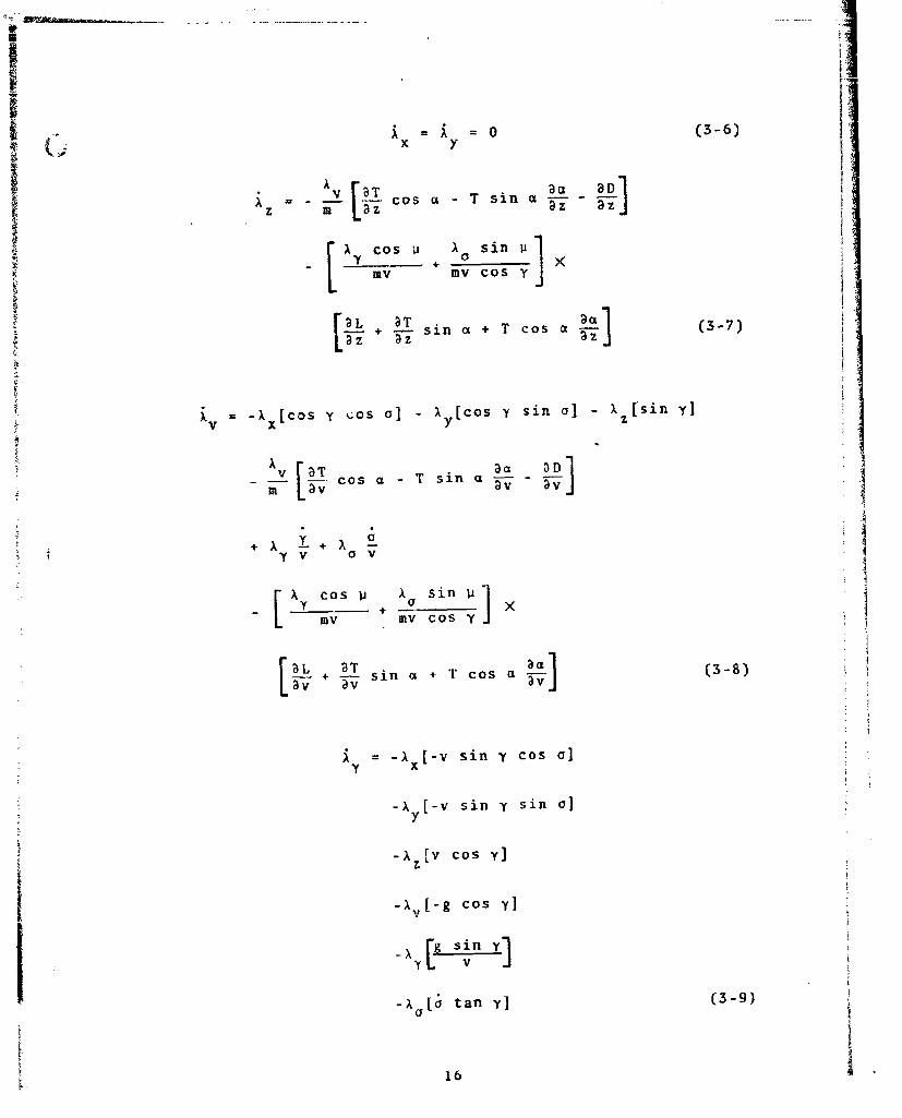
-= A --=0 (3-6)

A cos a T sin aT a 3D

z m L-5Z az ad

xCOS U A sin 1- l + a

lmV mV Cos y

-+ r- sin a + T cos a 1(37)z aT c

iv [ COS Y COS a] - y [cos y sin a] - Az[sin y]

x yz

_ -ý 3TCOS a - T sin a cv wv

•.y V 0 v

mV mv Cos "y

•-+ HT sin a +Tcos a a

lav av

= -A [-v sin y cos a]

y x

- P [v sin "y sin c]S~y

S-v [v c os Y ]

I- L-1 i ,,+[-g cos ] --

A = -A [-vsin y c-xA [v cs

-A [s tan y] (3-9)

16l

I ~~ = f-v ::sy sin a] (-0

-X[v Cos y Cos 0] (3-10)

The controls used are n, the load factor and p the bank

L angle. The evader's thrust is set to max throttle and is

then state dependent while the pursuer's thrust is zero.

Hence the unexpanded partial derivatives above become

with

L nW (3-11)

-- = 0 (3-12)9-z Wv

with

T = A + Bz + Cv (3-13)

3T •TB = C (3-14)3v

with

1 -z2 2D ,oe s(C + kCL ) (3-15)

-D - SD + 1 Ozv2s 2k CLSr0o L 3z

1 =8zv2s[D 2S- e - pe v s[C - kCL 2 (3-16)

with

KCL (3-17)

17

S• ,. •a CLIy= K v etc. (3-18)

with

nWC (3-19)L 1 -Az 2-Poe V S

CL CL- L(3-20)

av v

L BC (3-21)a z L

The load factor control is constrained and so account

must be taken of the effect of the constraint on the costate

equation.

C (n,zv) ? 0 (3-22)

C2 (n) > 0 (3-23)

where C1 is the constraint below the corner speed and C2 the

constraint above the corner speed and,

C1 = n 1 (z,v) - n 1= 0 (3-24)

C 2 = 6 - n z 0 (3-25)

Where the control is constrained

= - - H II •C. r7.- 7 Az z I z%- -.

i = - H - V (3-27)V V V

n H (3-28)n n

Hence

iz H H C (3-29)

S= H - HnC (3-30)

Vt v n v

for constrained load factor below the corner speed and since

the constraint above the corner speed is state independent

A -- H (3-31)2 Z

r A =-H (3-32)V V

as before. In the case of the pursuer the missile is con-

sidered to have sufficient control at all speeds of interest

that only the state independent constraint is in force.

For numerical purposes a Fortran integer variable "mu"

was used to switch the additional terms on ?nd off as neces-

sary in the costate equations so that as the load factor

selected by the control algorithm was constrained to the

state dependent limit "mu" was set to 1, otherwise it was

left at 0.

Optimal Contro!s

For an unconstrained control such as the bank angle

the first order necessary conditions for an optimal control

require that

19

H =0 (3-33)U

Hence

H = - -- [L + T sin ca] sin p (3-34)p mv

h [L + T sin a] cos p (3-35)mv Cos

The second order necessary conditions require that

H <0 (3-36)

for a maximizing player. Combining these two equations we

are able to define

oe,

sin e = (3-37)

ee S cos y +

y e

Y e ae

o e Ye (3-38)liXe = ¢( cos e2 e2

y+~ Ve ee

For the minimizing player we find

sin p = p (3-39)S¢(ypcos yp) 2 + X2

p p

-l cos YCos 4 ' (3-40)

P p pp

20

In the case of the load factors we solve for the uncon-

strained load factor that is a stationary control of the

Hamiltonian. Should there be an interior control that opti-

mizes the Hamiltonian we check the sufficient conditions to

ensure maximization or minimization as the case may be.

Where however there is no interior control that is a station-

ary control with respect to H we choose either maximum or

minimum load factor to achieve constraintd optimization.

For the evader then we consider the first order neces-

sary conditions

11 0 (3-41)n

H _ -T sin aCLn 3D

an Mn

+ m L •L + T cos a Cos CS

_____ FL •aa

my c+ s y ['n + T cos a sin p (3-42)

where

ac= t (KC _ L a(KnW/QS) (3-43)an an an

KW

aD - (C--+kC2os (3-441an in LJu

2knW2

QS

!

i and

- W (3-4S)

Thus

[-T si-K 2knW2

0[ sikn2 QS QS

k)y cos p. 4.Ac sin p ] [K](_6x [= + T cs I (3-46)

"c- [w + T cos QS

Substituting for cos u etc and making small angle approxima-

tions

A K2 ~2 2kW0 v V TK nW2 2knW2S

Q 2 S2 -QS J

+ W + L (3-47)QS y cos (y) 2 my

EA2A (c2 + a [QS+TK]QS

y (CosWvX (TK2 + 2kQSl (3-48)

For an interior control the second order conditions are

A [ 2k W2 ]H = - - +< 0 (3-49)nn m Q 2 2 QS

i.e., X > 0 for n, above, to be a maximizing control.

2I

22

j .s For a constrained load factor the choice is either max

vr mir. load faý..toc. 7he 1-amiltonian terms that containload factor dependent terms are

H1 = 2- (T cos a - D) + (2 CL + T sin a) cos ua my

+ (L + T sin a) sin v

my cos y

v(L+ Tsin a) 2 oi (T cos a- D) + X + - (3-SO)

(cos y)

For A > 0 we can look for an interior control and if

n so defined is too large we choose n fin max. For Xv S-

we find that our sufficient condition predicts a minimiza-

tion of H in some region of negative load factor, In order

to maximize the Hamiltonian we select n = n max for 1 < 0.

The exact opposite arguments are used to select the

optimum load factor for the missile. Thus, for interior

controls

22

n =-QS A ÷ P+2 - v (3-51)2Wp)

"p (cos y VP p

which requires X c 0 for an interior control to be posFible.V

Sufficient conditions for a minimum with respect to the

Hamiltonian are

H >0 (3-S2)nn

23 I

21

2kW2"H .. 3 Q.EA (3-53):nn MQS

Henc X A 0 for minima and following similar arguments

for the pursuer a3 for the evader we choose the constrained

load factor to be

n = nmax for >X v 1 (3-54)

and

n nmax for Av <0 (3-55)

Proportional Navigation Scheme

In order to check the validity of the results a propor-

tional navigation algorithm was produced for the missile and

used against an open loop optimal evasion scheme.

We expected to find that the proportional navigation

scheme (PN) would fly a similar course to the open loop

optimal missile but would not get as close to the evader.

For the purposes of the test the PN scheme was allowed

to use the exact current values of the vehicle velocities

and positions to measure the spin rates of the line of

sight. The line of sight was defined by two angles, one

an azimuth angle and the other the angle out of the hori-

zontal plane. For the Cartesian frame centered on the

missile as in Fig. 1 the two angles are respectively 6, '.

24

E

Fig. 1. Line of Sight Angles.

tan 4 = (3-S6)V-2 + ),2

•.Z - ! _ _ (Xx-yy,? (3-S7)2 2 )r7 Jx2 y 23

%f+ -2 -y X 3x + y

Similarly

tan 0 (3-58)x

2-- --2 (3 - 5 9)

2 .

SWe wish to fly the missile so that y p and aoP are

some multiple of and 8

y =RKI LCo gos sP- (3-60)

o=RK,2 Lsn (3-61)mv Cos y

Hence

tan RK2 (3-62)-K I C os -y

v

and then

L =RK26mv Cos -Y= nW (3-63)s in 11"

If n so defined ex4eeded 1S it was set at 15.

These values of p, n were then used in Eq (3-60) and

a

$WEq (3-61) to give the time rate of change of y and a for

sthe missile.

T!n the case where 6 is very small or zero the evalua-

tion of the load factor in Eq (3-63) leads to numerical

inaccuracies. In this case Eq (3-60) is used

l ' RK1 I + g o (3-64)

a g cos (6 v

Hence

IV. Results

TPBVP Solution Method

The results can be divided into two phases namely

(a) nominal saddle point solutions

(b) variations about the nominal solutiun.

Subroutine NSOIA was utilized in both phases. Firstly, it

was used to provide a one dimensional search for a point

on the terminal surface, and secondly it was used to solve

two point boundary value problems, both in the refining of

the nominal saddle point solution so as to minimize the

errors resulting from numerical integration and in the up-

dating schemes to solve the two point boundary value prob-

lem (TPBVP) at each update point. Appendix B presents a

short discussion on the principles of the subroutine and

on an aspect of the numerical integration of the state and

costate equations that is the probable cause of variations

in a Hamiltonian which should be constant.

Saddle Point Solutions

In order to produce a large number of saddle point

solutions covering a wide range of terminal conditions,

points on the terminal surface were found by selecting

eleven out of twelve of the terminal states and varying

the remaining state until the transversality condition on

H(tf) was met. Reference 3 provides justification for this

approach since it is shown that barriers do not occur in

the game formulation.

27

By integrating backwards from the terminal surface it

was possible to construct saddle point solutions to games

which ended at 30,000, 20,000 and 10,000 ft with final miss

distances from 0 to 200 ft and with a variety of track

crossing angles (TCA). TCA was defined as the angle b, tween

the missile and aircraft velocity vectors at tf By inte-

grating forward again to t it was found that there were

errors, due to the numerical integration scheme, and the

transversality ccnditions were not ,met exactly. These

could be reduced by letting NSO1A vary the initial costates

slightly until these errors in the transversality conditions

were reduced to some acceptable level,

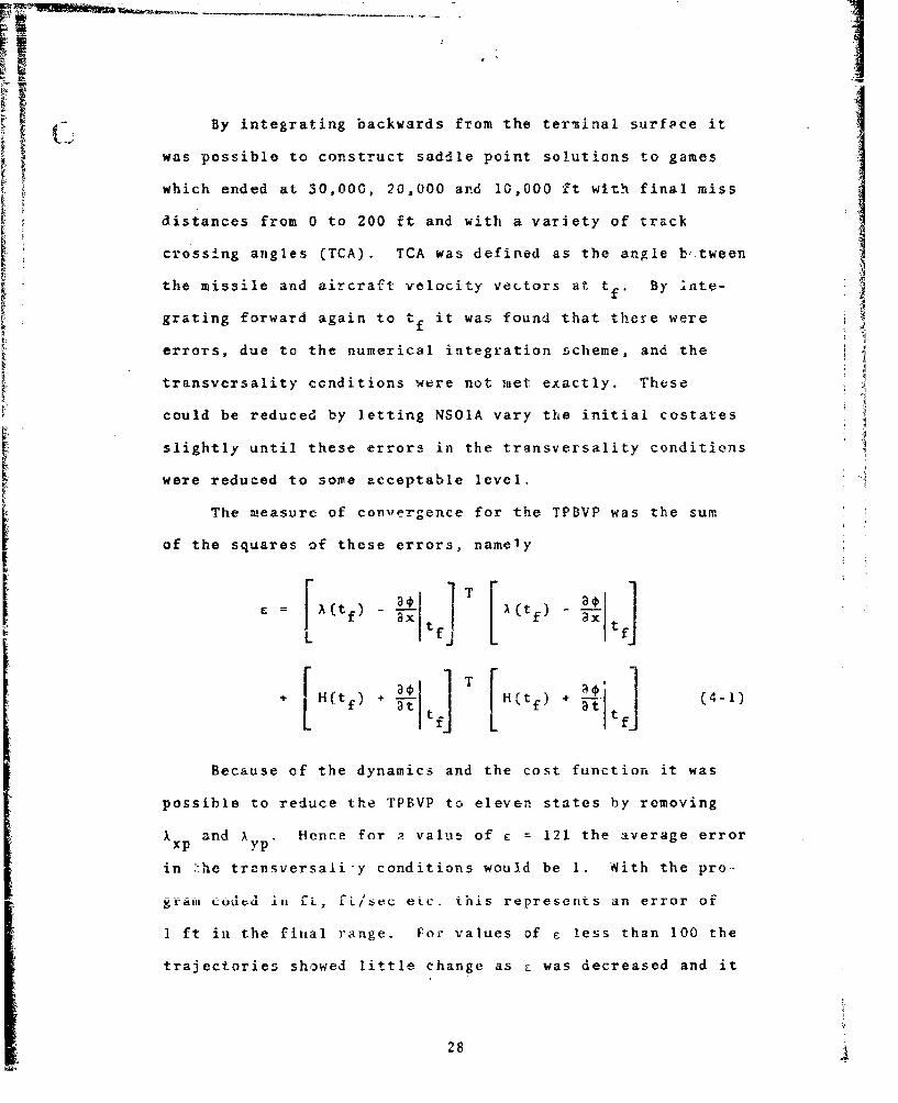
The measure of convergence for the TPBVP was the sum

of the squares of these errors, namely

[- Ac(tf) - tfj T (tf) - t

t) + Hrt- + . (4-1)

H(tf) -tf] [ tf

Because of the dynamics and the cost function it was

possible to reduce the TPBVP to eleven states by removing

Xp and yp. Hence for a value of c = 121 the average error

in "-he transversali-y conditions would be 1. 'With the pro-

gyaim cojud in 1L, CLi/sec etc. this represents an error or

1 ft in the final range. For values of c less than 100 the

trajectories showed little change as z was decreased and it

28

was possible to keep NSOIA searching until c was less than

.001 at which point the terminal miss distance was fixed

to within a fraction of an ine.i. c was therefore used to

define acceptable convergence in the solution of TPBVP's.

For refining nominal solutions c was set at 20 and for the

updating scheme c was set at 400 so as to reduce computer

time. In a typical updating scheme approximately 25 TPBVP's

were solved and it was necessary to sacrifice some accuracy

to keep total running time to a minimum.

Open Loop Controls

With final time free and with the cost function used

the open loop optimal trajectories looked realistic. The

optimal evader normally turns across the missile's path and

in most instances descends. The aircraft was kept subsonic

because polynomials representing load factor limit, maximum

thrust and drag as functions of height and velocity were

only valid subsonic. As a result the aircraft was usually

below its corner speed in the cases considered and by

descending it was able to turn faster. The aircraft also

gained thrust and load limit advantages by descending.

Both missile and aircr•'f, used maximum load factor along

smooth arcs to the terminal surface. This was, for nonzero

final range ,the point at which each had the same radius of

turn and the aircraft was on the inside of the missile.

The missile paid a large drag penalty using maximum load

29

factor and would typically give up 1500 ft/sec in velocity

during the 6 second engagement,

The initial relative position of the two vehicles

6 seconds away from termination varied from a beam attack

at 5000 ft range for a final range of 0. ft to 12,000 ft

with the missile about 400 off the front of the aircraft

for final ranges of 200 ft.

In all the cases studied interior controls were never

used and despite attempts to force interior controls by

utilizing zero final range and a TCA of zero and forcing

interior controls at tf when integrating backwards, interior

control solutions were never found.

The justification for free final time is not only that

it is more realistic but also for terminal pay off it is

essential for valid results as the following example shows.

The work of Ref 9 uses a comparable game model as the model

of this thesis and it presents one solution for an air-to-ll air missile using fixed final time. The cost functions are

different but the small difference should not affect the

game significantly. In the problem of Ref 9 a beam attack

at 30,000 ft results in the aircraft turning away from the

missile and both missile and aircraft use interior controls.

At tf S secs the missile is 1300 ft astern of the air-

craft flying a parallel trajectory. It appears that in

about 2 sees at most the missile will achieve a maximum

hit. The same problem under a free final time formulation

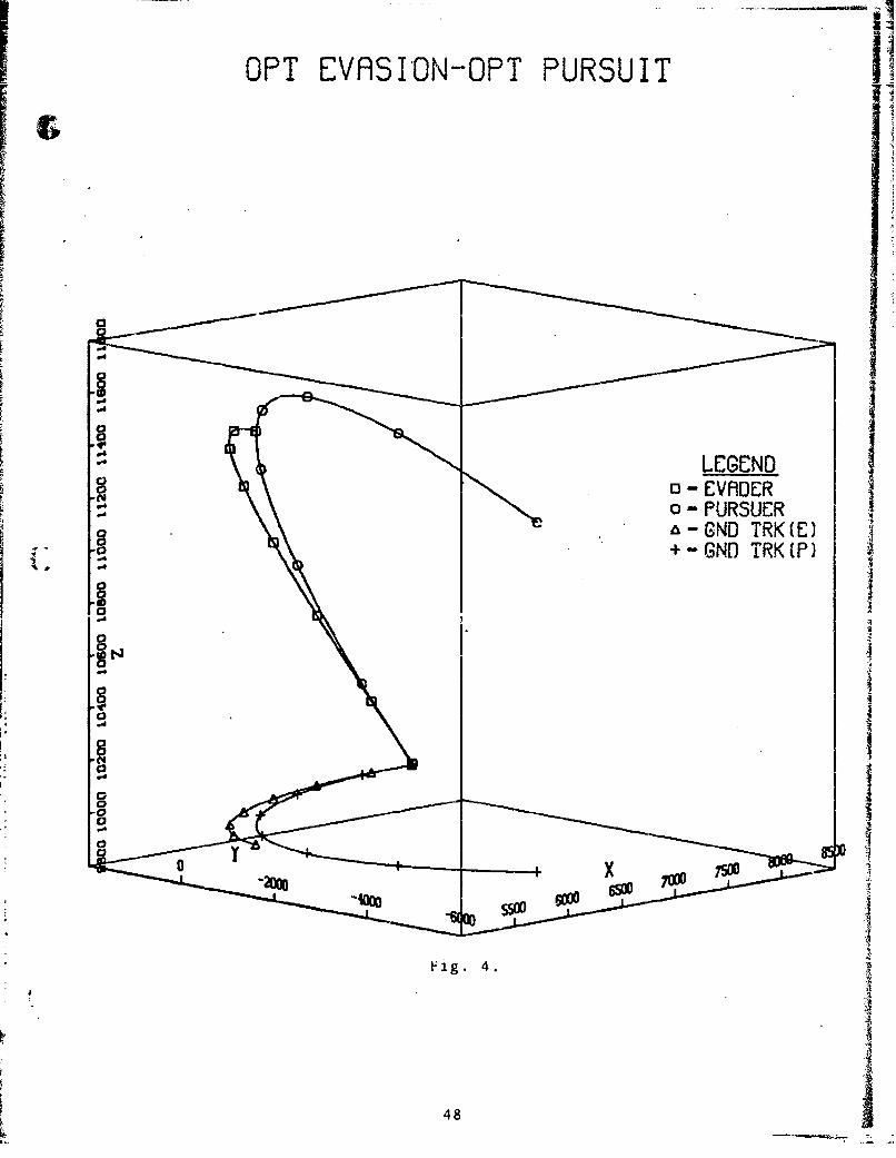
is shown in Figs. 2 anu 3. The 3D trajectory is given in

30

p

Fig. 2 with the ground tracks of the two vehicles plotted

on the bottom of the box containing the trajectories. The

bank angle selected in the saddle point solution is plotted

along with the proportional navigation (PN) choice of bank

angle. The PN plot represents the choice of bank angle

based on line of sight (LOS) considerations as the missile

flies along the optimal trajectory. The aircraft flies

across the path of the missile and dives. The missile is

then forced into a maneuver whereby it begins to fly to

the right of the initial position of the evader and then

continues to climb above the evader for an approach with

the minimum TCA it can achieve. Both vehicles use maximum

load factor throughout the 5.108 secs.

It appears that the fixed final time problem guarantees

the aircraft's safety provided R(tf) is nonzero. It also

does not prevent range going to zero at some intermediate

stage. The trajectory in Fig. 2 has a smaller final range

than that of Ref 9 in similar times and yet ultimately the

result of Ref 9 will be more in the missile's favor than

that of Fig. 2.

A selection of open loop saddle point trajectories are

shown in Figs. 4 through 15. For comparison purposes plots

are made of the bank angle selected by the missile on the

basis of optimal control and proportional navigation. Since

the missile flies along only one of these paths the bank

angle selection of the alternate scheme is not accurate.

In the very early stages the inaccuracies will be small and

31

Scomparisons can be made between the two schemes. The plot

of bank angle immediately following an optimum pursuit tra-

jectory plot is made along the optimum pursuit path.

Proportional Navigation Versus Optimal Control

The variations of optimal control (OPT), nonoptimal

control (NONOPT), and proportional navigation (PN) considered

(a) saddle point solution

(b) open loop OPT evasion versus PN pursuit

(c) updated OPT evasion v•rsus PN pursuit

(d) updated OPT pursuit versus NONOPT evasion

(e) PN pursuit versus NONOPT evasion.

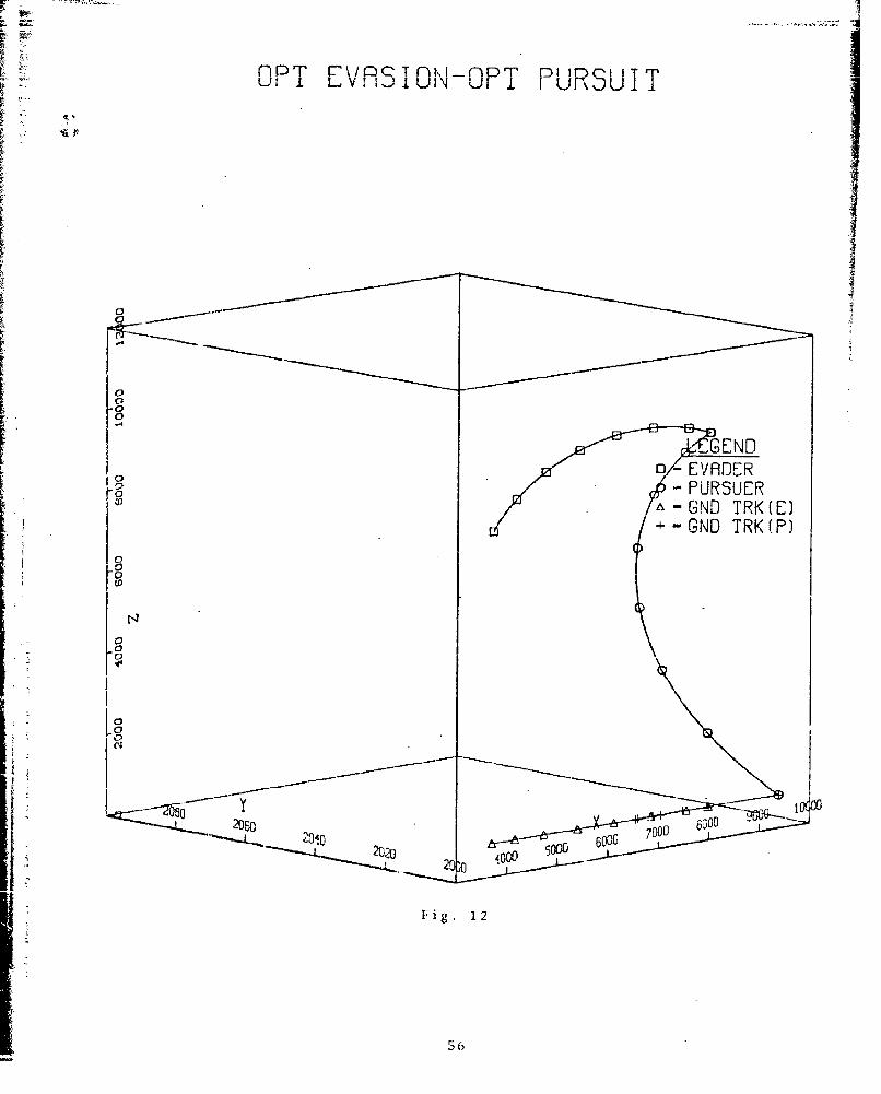
The open loop optimal evader results demonstrated that

for all but a few cases the open loop optimal evader gained

against proportional navigation. The few cases were the

problems where the saddle point solution lay in a plane ofconstant X or Y and hence bank angle was predetermined.

Since PN used maximum load factor in these cases the out-

come was the same as for the saddle point solution. Figures

12 and 13 are two such cases. Figures 16 through 23 present

two cases for comparison of open loop optimal control versus

proportional navigation for an open loop optimal evader.

In each case the open loop optimal evader gains against

proportional navigation. In this group o` figures the bank

angle selection of the two schemes when flown along the

proportional navigation path is given after the proportional

32

I £ navigation pursuit trajectory plot. Plots are also given

r of the rotation rates of the line of sight (LOS) whilst

guided by the proportional navigation scheme.

Tables II and III give the initial conditions for the

two cases presented in Figs. 16 through 23. Table I gives

the final ranges for the two cases for the optimal control

and proportional control missile against open loop optimal

evader.

Table IFinal Ranges for OPT and PN

Fig. No. Final Range

16 182

17 440

20 1.76

22 11

Tuned Proportional Navigation

An incidental result, on which little time was spent,

is mentioned here because it greatly improved the perfor-

mance of the PN scheme. For a given set of initial condi-

tions and for an evader playing the open loop optimal control

the PN scheme could be "tuned" to improve its performance.

The two navigation gain constants for PN had previously been

set to the same value. By introducing a ratio between these

gain constants considerable improvement in the performance

was achieved.

33

The case considered was the problem in Fig. 16. The

PN scheme used maximuw load factor throughout the flight

and only the bank angle differed between PN and OPT guidanc .

The bank angle selected by PN had similar characteristics

and so the initial bank angle of the PN scheme was b;:ought

closer to the initial bank angle for the OPT guidance. The

means of varying the PN bank angle was to select some ratio

for RKI:RK2, the vertical and horizontal gain constants,

For a ratio 1:2 the final range had been brought down from

440 feet to 207 feet which compared very favorably with the

OPT scheme result of 182 feet.

An example of the advantages of the tuned navigation

scheme is given in Figs. 24 through 27. The ratio used for

RKI:RK2 was 1:2 and this ratio was not optimized. It was

merely a first estimate of an improvement and since ratios

of 1:1.7 and 1:2.3 gave similar improvements 1:2 was used

to present the results. Figures 24 and 25 are the open loop

saddle point solution with the "tuned" proportional naviga-

tion bank angle plotted whilst flying the optimal trajectory.

Normal proportional navigation achieved a 478 ft miss and

with "tuned" proportional navigation the result was 191 ft

against the 173 ft for the saddle point solution. Table IV

presents the initial conditions.

Pseudo Closed Loop Guidance

For an open loop solution to be useful the evader must

play optimally or the open loop solution must be updated.

34

0 The open loop scheme was updated at approximately .3 sec

intervals throughout the attack by solving the associated

two point boundary value problem. The solution was considered

acceptable when the sum of the squares of the errors in the

transversality conditions was less than 400. The new solu-

tion could then be used to update the optimal missile attack-

ing a nonoptimal evader or an optimal evader escaping a PN

missile. This was an expensive process in terms of computer

resources and is completely out of the question for real time

guidance. It does however provide valuable information as

to the magnitude of the changes in the costates and demon-

strates what gain could be made in the "cost" for whichever

player was being updated.

The motivation for this approach is that a proposed

real time pseudo-closed loop scheme (Ref 1, 2, and 4) will

probably have to give up some of the realism of the model

for the advantages of a better behaved two point boundary

value problem. In order to test simpler models for their

ability to provide sufficient advantages over proportional

navigation, or in fact any other scheme, to warrant imple-

mentation, then some means of comparison is required. The

work of this thesis is therefore intended to provide a ref-

erence performance standard. Table V and Fig. 20 provide

a saddle point solution as the basis for the various compari-

sons that can be made. These are:

(a) open loop optimal evasion versus proportional

navigation

a

(} updiated optimal evcaion versus propcrtional

navigation

(c) updated optimal pursuit versus nonoptimal

evasion

(d) proportional navigation versus nonoptimal

evasion.

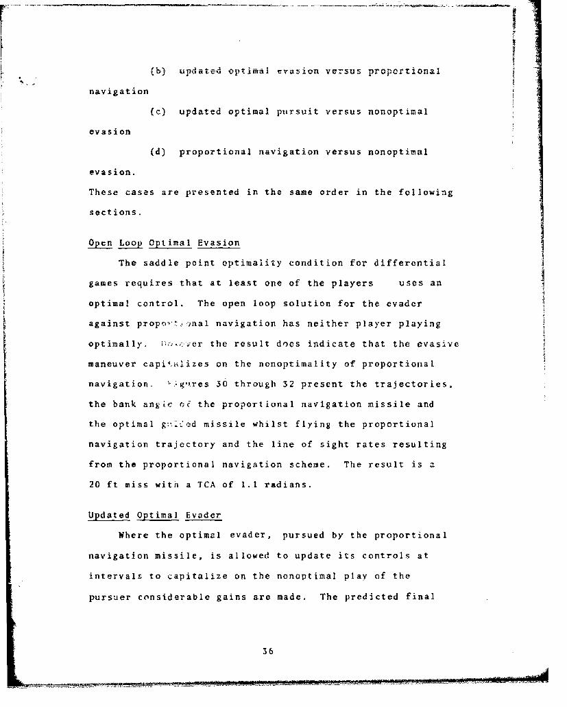
These cases are presented in the same order in the following

sections.

Open Loop Optimal Evasion

The saddle point optimality condition for differential

games requires that at least one of the players uses an

optimal control. The open loop solution for the evader

against propovz•. mnal navigation has neither player playing

optimally. Va,,,er the result does indicate that the evasivemaneuver capi4. lizes on the nonoptimality of proportional

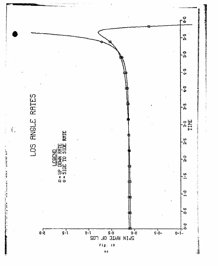
navigation. g.'.gres 30 through 32 present the trajectories,

the bank angie oe the proportional navigation missile and

the optimal g;Ktced missile whilst flying the proportional

navigation trajectory and the line of sight rates resulting

from the proportional navigation scheme. The result is a

20 ft miss with a TCA of 1.1 radians.

Updated Optimal Evader

Where the optimal evader, pursued by the proportional

navigation missile, is allowed to update its controls at

intervals to capitalize on the nonoptimal play of the

pursuer considerable gains are made. The predicted final

36

range, track crossing angle and the cost function assuming

the missile reverts to optimal control given by the TPHVP

solution at each update are given in Table VI. The range

R is in feet and the track crossing angle TCA is in radians.

The cost function and the degree of convergence are also

given. T is the predicted time to go, again assuming both

players play optimally, and the column T - t gives a compar-

ison with the column T to show how the game is extended by

the updating optimal evader to gain further advantage.

The entry at line 22 in the table is the final range (180 ft).

Figures 33 and 34 present the results for the updated optimal

evader. The bank angle selected by the optimal missile is

actually perturbed by being forced along the PN trajectory

in Fig. 34. It does show, however, that the PN scheme is

near optimal and that the solution to the TPBVP at the up-

date points was realistic.

For the case of the updated optimal evader the costates

are presented in tabular form in Tables VIII and IX. At

each update point the current values of the costates are

given in the "in" column. The values of the costates after

the return from NSO1A are given in column "out". The game

is then integrated forward to the next update point and the

current values of the costates are used as guesses and appear

in the "in" column. The change in costates between updates

is therefore the difference between the costates in the "out"

column at one update point and the "in" column at the next

update.

37

The close similarity between proportional navigation

I bank angle and optimal control bank angle in Fig. 34 sug-

gests that "tuned" proportional navigation may well have

made considerable improvements. Unfortunately, no time was

available to consider this case.

Updated Pursuer

These cases are those where the missile is allowed an

update at .3 second intervals against a nonoptimal evader.

The evader flies max g load at a bank angle of 90* as a

nonoptimal evasion.

Flying optimally the evader could only achieve a final

range of 1.5 feet. The final time was 6.004 secs. During

the updating computer run a less accurate solution was taken

to be acceptable. The first call to NSOlA solves the initial

two point boundary value problem and the time to go was set

at 6 sec. The answer was acceptable within the new accuracy

requirements but the small change in time alone of 4/1000

secs changed the terminal miss to 4.4 feet with a sum of

squares of the transversality errors at 240. The results in

Table V represent a solution with an error of 14.

Table IX gives the results from the computer run. The

overriding factor in determining the number of updates, the

acceptable accuracy and the maximum allowable number of

iterations in the solution of the TPBVP was the central

memory time requirements. These results are therefore not

ideal in that the trade offs between accuracy and central

i3

W1

memory time have not allowed convergence in many instances.

The instability cf the resulting controls reflect this lack

of convergence but at intervals the solution converges and

the missile promptly makes up lost ground. However, in the

last time period the missile is flying open loop against a

nonoptimal evader who is able to double his miss distance

during this last critical stage.

An interesting aspect was the fact that at updates 12,

13, 14 the l1th update open loop solution remained accept-

able. With no update made the evader gained ground against

the missile. Figures 35 and 36 represent the trajectory and

the optimal bank angle respectively.

Proportional Navigation with Nonoptimal Evasion

In this case the nonoptimal evasion maneuver is used

against a proportional navigation missile. The result is a

20 ft miss with a TCA of 2.02 radians which is more in the

evader's favor than the open loop optimal evasion. Where

neither player plays a game optimal strategy the saddle point

optimality is not meaningful. It does suggest that only a

poor estimate of the open loop evasion strategy makes

reasonable gains against proportional navigation. The up-

dated evader however makes considerable gains for this

problem. That the updated optimal evader cannot always

make such startling gains can be seen in Tables X and XI.

These two problems are based on saddle point solutions that

ond in similar ranges but different TCA's. In the first

39U

case the saddle point solution is given in Table III and

Fig. 20. The bank angle plot of Fig, 21 indicates the near-

optimal nature of proportional navigation. As a consequence

the updated evader can only extend the range to 22 ft.

However for the case of Table XI the updated evader makes

considerable gains against proportional navigation. The

saddle point solution is given by Fig. 6. The 1.73 ft of

the saddle point solution is converted to 370 ft by the up-

dating evader.

Summary

The problems associated with the solution of the TPBVP

for very small final ranges is reflected in the instability

of the updating scheme for the pursuer. Where he has an

open loop final range that is small, noncptimal play on the

part of the evader is difficult to convert to a decrease in

the payoff. Where the saddle point solution has a much

larger final range, initially, while the pursuer is convert-

ing nonoptimal play by the evader into a decrease in the

payoff, the TPBVP is amenable to updating w;ithin the number

of iterations allocated. However as the final range gets

smaller the TPBVP becomes more awkward. In one case the

pursuer converted a 240 ft final range to .7 ft at some

intermediate stage. The updating scheme was able to keep

the final predicted range to about 2 ft despite lack of

convergence at some update points. However in the last

40

( phase under open loop control the predicted final range of

2 ft became 11 ft.

The updating evader has this aspect in his favor since

he is continually increasing the final range, The problem 3becomes more well behaved and hence easier for hin, to update.

Even if he doesn't update the open loop saddle point strategy

provides scme small gain against proportional navigation

missiles.

In the cases considereu no interior controls were found

even for proportional navigation. This is probably because

for an open loop optimal evasion or even for a rough approx-

imation to optimal evasion the missile is forced into maximum

g maneuvers. Hence proportional navigation loses because

of its inability to lead or lag its bank angli, based on

considerations other than the immediate line of sight rate.

Many cases in this thesis show bank angle patterns very simi-

lar to optimal control with only a constant offset. In

other irstnnres, Fig. 3 for exampl, there is considerable

difference in the dynamic behavior, even though at a later

stage the bank angle selections are essentially the same.

The gain constants for the PN scheme were normally 10,

This represents a performance for PN beyond the current

capabilities.

41

rir I

V. Conclusions and Recommendations

Conclusions

This thesis compares the principle of proportional

navigation to differential game optimal control. But for

a few cases presented where launch conditions are very

favorable to the missile, proportional navigation normally

pays a considerable penalty, in terms of the cost function,

in that the missile has the energy and the maneuverability

4n greatly improve the p7obability of kill under optimal

control. The realistic dynamics used in this thesis are

unlikely to provide the basis for a pseudo-cloLed loop

optimal control scheme as suggested in Refs 1, 2, and 4.

However the considerable 'ains that can b, made suggest

that simpler models may be used so as tc :ompromise between

gains in the payoff and in achieving a real time capabi!ity.

It appears that the optimal evader has most to gain

using this scheme since the numerical problem; improve as

the final range increase3. The open loop control is effec-

tive against proportional navigation so that any failure

to update tha control does not relinquish existing gains.

Whereas any failure to update the missile control increases

the final range.

Lastly I conclude that the subroutine NSOlA is a power-

ful means of solving the TPBVP' a.s.ciatcd. with saddle

point solutions. Considerable care should be used in

selecting the parameters that control NSOA's pecformanze

42

and in this respect NSO1A remains in the same class as

most other schemes in that a good understanding of the

nature of the solution is essential to obtaining a solu-

tion, no matter how powerful a numerical method is used.

Recommendations

It is recommended that further work in this subject

should concentrate on finding simpler game models that

behave in the same characteristic manner as the nonlinear

model of this thesis. Since interior controls have not

been found it may be possible to fix load factor at its

maximum value and reduce the problem to a single uncon-

strained control in bank angle for each player. Under

these conditions a simpler drag model may well prove suf-

ficiently accurate. If a simpler model produces similar

behavior then a pseudo-closed loop real time optimal

guidance scheme may well prove to be possible for simula-

tion purposes if not eventually for missile guidance.

43

IJBibliography

e1. Anderson, G. H. "A Transition Matrix Method forGenerating New Optimal Closed-Loop Solutions toNonlinear Differential Games". Preprint of InternationalFederation of Automatic Control - International Federationof Operational Research Symposium on Optimization Methods,Applied Apects, October 8-11, 1974, pp 27-35.

2. Anderson, G. M. "A Real-Time Closed-Loop Solution Methodfor a Class of Nonlinear Differential Games", IEEETransactions on Automatic Control. AC-17:576.

3. Anderson, G. M. "Minimax Range/Barrier Trajectories andTheir Application to Pursuit-Evasion Combat Problems".Proceedings of IEEE on Decision and Control Theory,Phoenix, Nov 1974.

4. Anderson, G. H. "A Near-Opt-mal Closed-Loop SolutionMethod for Nonsingular Zero-Su" Differential Games".Journal of Optimization Theory and Applications,13:303-318 (March 1974).

5. Asher, R. B. and J. P. Matuszewski. "Optimal Guidancewith Maneuvering Targets". Journal of Spacecraft, Vol.11, No. 3:204-206 (March 1974).

6. Bryson, A. E. and Y. C. Ho. Applied Optimal Control.Waltham, Massachusetts: Blaisdell Company, 1969.

7. Garber, V. "Optimal Intercept Laws for AcceleratingTargets". AIAA Journal, Vol. 6, pp 2196-2198 (November1968).

8. Isaacs, R. Differential Games, New York, New York: JohnWiiey and Sons, 1965.

9. Leatham, A. L. and U. H. D. Lynch. "Two NumericalMethods to Solve Realistic Air-to-Air Combat DifferentialGames". 12th Aerospace Science Meeting of AIAAWashingtoTn,-_eb 1974.

10. Powell, H. J. D. "A Fortran Subroutine for SolvingSystems of Nonlinear Algebraic Equations", NumericalMethods for Nonlinear Algebraic Equations, edited byPhilip Rabinowitz, New York: Gordon and Breach SciencePublishers, 1970.

44

Append ix A "

Tables and Figures •!

45 I

OPT FVASI ON-OPT PURSUIT

SUS

I(E)GN RKP

3 20

.46

OLfl

CDL

cr~ U7

co:

.1-of

ZD

IL]?

CU,

oOO60 OO6Sl 0.01 O*OS O -j O.OS- 0-001- O-0sl-. O0E-00

Fig. 3

47

OPT EVASION-OPT PURSUIT

EVDE

0 PRSE

tN RKE

-GND TRK (P)

484

f IOf

Z Vr);

00-

IL) 00La

CD

-D U

Cr)0::

VCLiCD

O-Ooz 00OSl 0001 00os 0.000-s- 0-1OO~-Os-ooz

Fig. s

OPT EVRSO'QN-OPT PURSUIT

LEGENDo - EV9DER0o- PURSUER

a -GND TRK(E)+-GND TRK(P)

Fig. 6

so

a_

000

CD,

a:

co

EIn

CD

* ZD

Cr)

15

OPT EVASION-OPT PURSUIT

+ -GND TRK(P)

j Fig. S

Ifimm

(_ m

0 0

cz

Ir) LiCDCL

CrC)

0Fii 9

OPT EVR9SION-OPT PU]RSUITT

LEGENDo EVA9DERo - PURSUER

G-ND TRK (E)+ GND RK (P)

0

Fig.. 10

1 S4

w Iw_R3

0-Q

LLI 00CC,

a7:

CLf

co:z o

uin

C('

CD

0-8 -9 C l)I 0! o0 .! .3, Oo 0-

TIN NY

Fig. 11I;-4

LLs

flfDT F'\IMC Tm ~n DT r~r i~ci~LVH1UI4 l 1 PURS)UIT

P0

GEN

0 VAE-PRSEA-N TKE

00

600002 O~a 700 50000j 202* 0 400

Fig. g 12

56

nlPr EVASIUnj-GPT PIUFSI TIr

I A -i fI%-"A A

LEGEND TV

EV9E

ac

2f 50 60

57

OPT EVASION-OPT PURSUIT

LEGEND-EVADER

0 -fURSERAGNU ¶FRK(E)

+i--GNU RKVP)

11

130

Fig. 14

58

C3IF

mm

U)VMcz

CDs

L 3 OU 0 6

CDC2

O-Oof O-Os 0-0 Ocj-0.0'r- 0 0o

Fig'. 4

59o

Table II

Saddle Point SolutionState Evader Pursuer

x 4972 ft 9199 ft

y 2986 ft 10260 ft

z 33150 ft 33170 ft

v 706 ft/sec 2219 ft/sec

y - 846 rads -. 619 rads

o -. 632 rads -2.41 rads

A209 -209x

A 211 -211yA180 -211

zA 179 2563

v

A 681248 -607926y

A 847488 -1478936

60

OPT EVAISION-OPT PUIRSUITT

LEGENDo - EVADER0 - PURSUER

ei ~A -GND TRK (E:)+GND TRK(P)

Fig01

.6Q

~ N~yPURSUIT

pFiF

/62

F6tE- D9

a-)

0-~E--4OC

a~roc0I

CE)l

GZ DcU,

ci9Cd2:L

0:CD

CD

r - T - C2U-0t 009 0 or I -OE 000 a G 0 09 0 -; -oz 0 &

Fif iD6

16)

ICI

LEL

cHic

Ca c3Dr

x E- c

1464

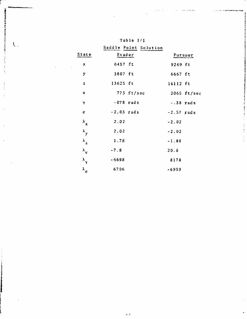
Table Ifl

Saddle Point Solution

State Evader Pursuer

x 6457 ft 9249 ft

y 3807 ft 6667 ft

z 13625 ft 16112 ft

v 773 ft/sec 2065 ft/sec

y -078 rads -. 38 rads

c -2.03 rads -2.57 rads

A 2.02 -2.02x

A 2.02 -2.02y

A 1.78 -1.88z

A -7.8 20.8V

A -6698 8178YAt 6796 -6959

0

I.c

r-Vj~f T'

0 0- PURSUCRA~- ND TRK(g)-GND TRK(P)

Fig, 20

66

U 0,

LJn C)CLaDo

coco U

Z:)0-)

0 -*Lc'.

U~lp

CDCC)Co

3ýSNU

Fig-2

OPT ,PkqTnKi-pRnFlP MRV PUIRSUIT J

o0-PURSUER

-GNIJ TRK (E)+ -GND TRK(P)

Fig. 22

68

cL2

Q 00

LI 00

CD 4

IA<I44

D aS :o -s 00 D-S- 001 -S' -31SNIU NN

Pi% 2Q6

Table IV

Saddle Point Solution

State Evader Pursuer

x 4936 ft 9341 ft

y 3013 ft 10358 ft

z 33198 ft 33326 ft

v 703 ft/sec 2235 ft/sec

y -. 84 rads -. 62 rads

a - .64 rads -2.43 rads

A 200 -200x

A 199 -199y

A 171 -201z

A 174 2473V

A650585 -554617

A 814617 - 14099b6

OPT EVASION-OPT PURSUIT

LEGEND9~o -EVADER

o - PURSUER

G-DND TRK(P)

Fig. 24

E- :DVI)

C.D DccL

LiD 00

C9>

C3j

CD :aT--

CL0

(n4

LLI)

CD

DLCiDOT DOE -s 00 Oo- O- - DDl -0:

KOPT EVASION-PROP NVPURSUIT

o-ENVfER0- PURSUER

+-fND TRK(P)

s0x

.0......... .... t.]..... .......

Fig. '16

C0

ILt

t C)

.1C CLJ

:I I

000

CD)

CEa

CLiCD

O f

cii

cD .1-

OL

CD

Z -I

.. .• . .......

J-10 __I [-

O.O (Y 0t 'S 0 Ji~OOT "~-~O

:mu~~ 13_ LoI

Table V

Saddle Point Solution

State Evader Pursuer

t =0 tf =6 t0 =0 tf =6

x ft 4178 8003 10920 8002

y ft 4435 1999 10242 1998

z ft 11123 10003 7782 10002

v ft/sec 849 799 2491 999

y rads -. 5 .1 -. 29 1.08

o rads -1.2 .0 -2.18 .79

Costate

A 2. 2. -2. -2.x

A 2. 2. -2. -2.y

A 2.02 2. -1.77 -2.z

V 2.3 0. 13. 0v

A 5533. -8.4 -23734. 5.6

A 12518. 3.4 -10647. -304

1o .... 1oOPT EVSO-OPT PURSUIT

EVAIO

LAG

Ii a

0

000

Fig. 28

000

cn

CL Lr)

cD LiICD

F- 0 C0

CDDQ

LLL C3 0

Fig. 9

OPT EVASION-PROP NAV PURSUITI

LEGENDo -EVADER0 -PURSUERA -GND 71RK(E)

+GNO 7RK (P)

Fig. 30

0- (r0

CDCO

LL]Q

CDa

CC>

cx

z)l'r

cLLnrCD

LLe

J71,NU )NMU9Fig, 3.1

VIM

coo

CIMn

LEL

-]-

HE cc:Ct)t

CD:

El3 c 0

~~(r)

301 JO IUý 01JFig. 02

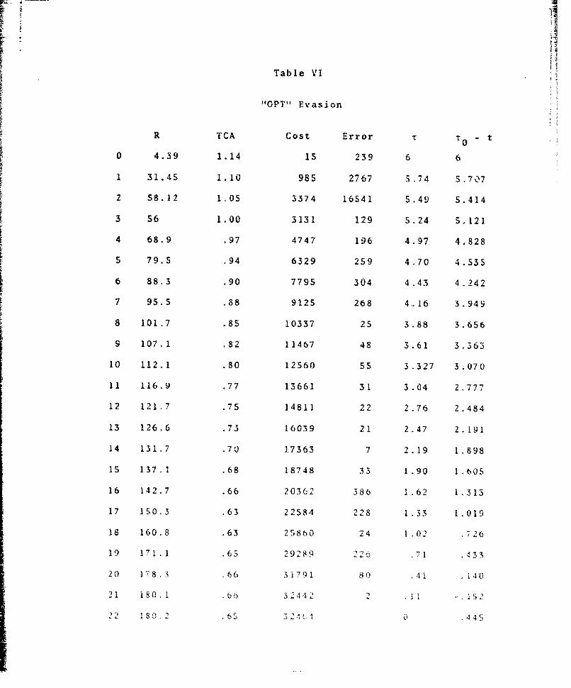
Table VI

"OPT" Evasion

R TCA Cost Error T T t

0 4.39 1.14 15 239 6 6

1 31.45 1.10 985 2767 5.74 5.707

2 58.12 1.05 3374 16541 5.49 5.414

3 56 1.00 3131 129 5.24 5.121

4 68.9 .97 4747 196 4.97 4.828

5 79.5 94 6329 259 4.70 4.535

6 88.3 .90 7795 304 4.43 4.242

7 95.5 .88 9125 268 4.. 16 3 .949

8 101.7 .85 10337 25 3.88 3.656

9 107.1 .82 11467 48 3.61 3.363

10 112.1 .80 12560 55 3.327 3.070

11 116.9 .77 13661 31 3.04 2.777

12 121.7 .75 14811 22 2.76 2.484

13 126,6 .73 16039 21 2.47 2.191

14 131 .7 .70 17363 7 2. 19 1 .898

1i 137.1 .68 18748 33 1.90 1.605

16 142.7 .66 20362 386 1.62 1.313

17 150.3 .63 22584 228 1.33 1.019

18 160.8 .63 25860 24 1.02 .726

19 171.1 .65 29289 229 .71 433

20 178.3 .66 31791 80 .41 .140

21 180 .1 66 324,2 2 ! .52

22 180.2 .65 321 2 0 445

OPT ENASION-PROP NAV PURSUIT]

oE VAIDER0 -- FUR3UER

A-OMJ TRK(E)04 + --GND TRK(P)

I o

ZDD

0 =) 0

I I

CD

:z

cr-4

LU

C)1

0-M -OS 0-01 009 .C. .02 ()OotC)'S I

Pi .,3

830

Table VII

Evader's Costate History

A zx 1' z

III Out I n 0." c I n Out

0 1.99 1.99, 1.9M9• 1.98 2.00 2.00

1 1.99 13 1.93 12 2.00 12

2 13 42 12 36 12 30

3 42 71 36 57 39 63

4 71 90 5 7 63 77

5 90 108 67 74 77 89

6 108 123 74 78 89 98

7 123 136 78 80 98 •0E

8 136 148 80 81 105 111

9 148 160 81 80 111 115

10 160 171 80 78 115 119

1I 171 133 78 75 119 122

12 183 195 75 70 122 125

13 195 208 70 64 125 127

14 208 222 64 56 127 128

15 222 237 56 46 128 128

16 237 252 46 31 128 126

17 252 279 31 -14 126 109

18 279 302 -14 -65 109 88

19 309 314 -65 -121 88 61

20 314 311 -121 -169 61 37

21 311 305 -169 -189 .37 27

84

Table VIII

Evaier s Costate Hiitort ly

V Y C

In Out In Out In Out

0 -12 -12 6518 6518 12453 12453

1 -10 -60 6596 42452 11881 75319

2 -48 -136 42496 134076 71S1! 223344

3 -104 -140 132856 217525 210976 341921

4 -95 -87 213396 262847 321156 391235

5 -40 -14 255299 294299 365283 416446

6 30 66 28•10 11.3289 4??94•

7 106 146 298234 320259 389568 413679

8 178 221 301699 318129 378058 394004

9 245 286 2Q6411 308454 356930 366781

10 299 342 384018 292586 328969 334346

11 343 387 265927 271695 296262 297838

12 377 420 243345 246556 260503 258884

13 398 441 217102 217828 222745 218235

14 408 449 187930 186023 183983 176725

15 403 442 156455 151907 !45141 135257

16 384 416 123596 ]17086 107267 95047

17 346 386 91235 77421 71922 41846

18 302 326 57999 42076 30068 515

19 233 241 29536 '5017 339 -- 24454

20 141 141 9261 1491 -13174 -26901

21 39 39 696 .168 -6844 -8703

Table ix

"OPT" Pursuit 11Update R(tf) TCA Cost Error v0 - t I

0 4.4 1.14 151 239 6 6

27 1.22 780 4931 5.64 5.7072 44 1.4 2003 11645 S 2 5.414

3 8.6 1.55 73 3752 4.8 S.1214 17.4 1.55 303 2086 4.41 4.328

5 1.19 1.49 .64 2109 4.07 4.535

6 4.18 1.46 16.49 1995 3.72 4.2427 1.40 1.6 2.67 82T 3. 17 3.949

8 2.5 1.87 9.26 254 2.69 3.656I 9 .95 2.01 5.17 65 2.31 3.363

10 9.04 2.01 85.9 390 2.02 3.070

11 6.942 2.06 52.9 37Z 1.70 2.777

12 4.8 2.06 27.9 195 1.41 2.484

13 1.91 2.06 8.39 36 1.12 2.19114 S.66 2.06 36.8 191 828 1.898

15 6.19 2.07 43.2 202 .532 1.605

16 6.33 2.08 45- 220 .239 ].313

17 13.03 2.08 164 - 0 1.019

86

INnN nP-,' £ýVASIQN-OPT PHR5UITT

LEGEND

CVF.DER

PU 'RSUERAGND TRK (E)+C-ND TRK(P)

I-ig. 35

87

LCL

Co

U7

CD

7Z)

IL

O-U 0-.ost oo0or Oo- oos 0 n -os-o- o-o)sr-o()oo?-.

D ~T r I~C T n M r -)r-cm 1 1 N Ift-- I 1ý

LEGENDD-E£VADER'o-PeURSUER

A -GND TRK(E)+ -GND TRK(P)

Fig. 37

1-I 00

_jn

CE)0

cn9

Co2

ciFig 38t

C>

ELLciZr

CD C

n: Li X

00

CSC5

L~MM

-JQC)

0.0 S--0*-t

SolJO 1UýNIdJS

91

Table X

fWT" Evasion

TCA Cost Error T T0

0 1.7S .086 -6.95 is 6 6

1 11.8 .04 131 2205 S.77 5.76S

2 12.7 .06 151 1357 SS6 5.531

3 10.0 .06 90 29S S.38 5.296

4 11.6 CIS 124 105 S.2 5.063

5 15.5 .05 232 421 4.99 4.828

6 15.0 .05 216 176 4.81 4.S93

7 15.9 .04 245 184 4.61 4.359

a 16.9 .04 21-7 141 4. 41 4.125

9 17.2 .05 287 112 4.21 3.891

10 17.S .05 297 141 4.00 3.6S6

11 17.6 .05 302 219 3.78 3.422

12 17.7 .06 304 is 3.56 3.188

13 17.7 .05 304 249 3.32 2.953

14 17.7 .06 304 136 3.09 2.719

is 17.8 .06 307 6 2.36 2.484

16 18.0 .06 315 291 2.62 2.250

17 18.3 .06 3 2.i 6 17 2.39 2.016

18 18.7 .06 340 68 2.16 1.781

19 19.1 .06 200 1.92 1.547

20 19.3 D7 362 257 1.69 1.313

21 19.8 o7 382 26S 1.46 1.078

22 19.4 .07 368 176 1.23 .844

23 19.8 .07 381 242 1.00 .609

24 21. .07 432 287 .76 .375

25 21.4 .07 448 281 .52 .141

26 21.9 .06 472 235 2' 9 .094

92

Table XI

"OPT" Evasion

R TCA Cost Error T - t

0 1.73 1.12 -1.3 .5 6 6

1 86.8 1.06 7529 34742 5.82 5.765

2 164 1103 27127 104577 5 65 5 .531

3 125 .968 15677 329 5.33 5.296

4 159 .917 25455 369 5.37 5.0635 190 .868 2 282 30 5.20 4 .828

6 218 1820 47579 86 5.02 4.593

2 242 .775 S8881 84 4.83 4.359

8 264.2 .732 69819 148 4 64 4 .125

9 283 .693 80106 297 4.44 3.891

10 299 .657 89522 75 4.23 3.656

11 312 .625 979ii 130 4.02 3.422

12 324 598 10c!71, 67 3.80 3.188

13 333 577 111295 260 3.56 2.953

14 341 .56 116291 120 3.31 2.719

1s 346 55 120242 8 3.07 2.48416 5Sl .54 123256 117 2.82 2.250

17 354 .54 IS443 28 2 .57 2.016

18 356 .53 126920 189 2.32 1.781

19 357 .53 127806 172 2 .07 1 547

20 358 53 128231 157 1.82 1.313

21 358 53 128350 43 1.59 1.078

22 358 .53 128362 7 1 .35 .844

23 353 53 128540 104 1 .12 .609

24 359 .52 129242 25 .91 .375

25 361 .51 130932 1 .69 .141

26 366 .48 133954 39 .48 - .094

27 371 .45 871 204 25 - .328

93

t?

Appendix B

Numerical Aspects

TPBVP Solution Method

A saddle point s(.lution to a differentix al game for.:u-

lation is defined by a two point bolndary value problem in

the form

A f(x,Xt) x(t 0 ) X X 0

X = g(x, ,t (tf) -

Z = free l-Utf) -4t( (B-i)tf

where there are n+I u ."nowns at t 0 , namely I(t 0 ) and tf and

at some time t chere are ntl relationships that must hold.

The problem could be more generally stated as follows,

F(x) = 0 (B -2)

where x estimates of n¼l unknowns in Eqs (B-I) and :hr

vector function F represents the relationsýhips that must

hold to some acceptable degree of accuracy it time t The

solution of Eq (B- 2) provides the appropriate unkriuo.ns at

time t 0 such that if both players play optimally throughout,

the terminal conditians for the game wi 1l be ,set. Fval'.ia

tion of F requires integration of the system d>namic using

some present estimate of the -N(t 0 ) for a period (tf -tj0

given a current estimate of the final time t Now consider

94

the minimization of the scalar cost function

mrin FTCx)F(X) J* (B-)x

The first order necessary conditions are

3J* 0 = 2 FTF (B-4)ax - x

the solution of which is either

FT =0 T

(B-S)F = [0]x

Another solution exists when F is singular for some F 0 0.x

Using these three possible solutions together with Eq (B-3)

the three solutions can be separately identified as follows

(a) FT x)FCx) < C (B-6)

(b) FTF > kFTF (B-7)x

Cc) IFxI = 0 (B-8)

In (a) the solution of Eq (B-2) has been achieved to

within e. In (b) the gradient of F, Fx is such as to predict

a very large step 6 in a Newton-Raphson searqh for the minima

of FTF. The constant k allows some control over what is and

what is not an acceptably large step. Normally in gradient

search techniques a singular matrix P precludes finding the

gradient direction unless the generalized inverse of F is

used.

-.. 9 5 - • . ..19-,->

A Fortran subrouti-.e published at Ref 10 searches for

a solution to Eq (B-2) until F'F is less than some :, w ich

is Part of the c-lling parameters. It initially estimates

F by numerical differentiation using a user supplied stepX

size and after taking the inverse of F thereafter usesa-l

approximations of F based on the steps it takes in thex

search. Should the gradient scheme define an unacceptably

large step, as controlled by k in Eq (B-7), then control is

returned to the calling program. By continuously approxi-' -1

mating F - then the problems associated with Eq (B-8) arc

avoided.

Since the scheme uses an approximation to F it tends

to take cautious steps in the search for a solution so that

the assumptions in making the approximation are not violated.

Changes in this step size are made if the predicted value

of F(xt-6) anr the actual value are either- very cdoz.e in

which case A the step size is increased or wildly different

in which case A is reduced. In the algorithi,' the Newton-

Raphson step is calculated and if this is less than or equal

"to A it is used direct-ly. If this is not the case the algo-

rithm predicts the optimum step siz-e in the direct2on of

steepest descent assuming that it is searching on a quadratic

surface. This step size is compared with A as before.

Should neither steepest descent nor Newton-Raphson predict

a step size less than A a combination is used to calculate

S*." or a i n a. direccicon somewiere between the two.

96 3

l.

Because the scheme has -t pseudo cost function F TF

which has a minima at the solution of F(x) = 0, it retains

the value of x that has produced the smallest value of FTF

and on an error return to the calling program usually re-

turns this "best" value of x no matter how far away the

current estimate of x may be.

This then is the algorithm that has been used through-

out to solve the two point boundary value problems that

represent the saddle point solution.

Numerical Problems

The Hamiltonian in the game formulation was independent

of time and hence

dHH 3 HT dx ;HT d• atdt 3x dt DX dt

M T dX a lH- ff÷ --

f + dt 4t

- iTf 4 fTi = 0 (B-9)

The Hamiltonian at final time was zero and hence should have

remained so. When a set of states, representing the termina-

tion of a differential game with a miss of 100 feet in each

direction, was integrated backwards in time, the Hamiltonian

oscillated rapidly and then gradually settled at some value.

The differential game was coded in an unnormalized form,

that is positions in feet, velocities in feet per second,

etc. Even when the integration step size of 5 jsec was used

97

I:i

and the Hlamiltonian oscillated, but to much smaller limits

than previously, the trouble seemed to lie in the integra-

tion and not the equations being integrated. The integration

routine used was a 4th order Runge-Kutta to start and there-

after a 4th order predictor-corrector. The choice of fixed

or variable step size could be made in the calling parameters.

For a variable step size the routine would increase or de-

crease the step size as necessary to keep the error bound

below some given value. As the step size required changing

the scheme would use Runge-Kutta to start afresh before

moving to predictor-corrector integration. It was noticed

that it was always the Runge-Kutta steps that produced the

oscillation which would then settle down considerably during

predictor-corrector integration. When, in variable step

size mode, the Runge-Kutta scheme was used to start afresh

after each change of step size, back came the oscillations.

With a miss distance of some 176 feet the values of X (tf)Y

f

and A a(tf would lie between +10 and -10 but their slopes

would be of the order l.ES. Since the states and costates

were being integrated by a single routine the range of

slopes that the one routine had to handle was from -IES to

+IES. The value of A was iargely aerermined by such termsY

as A v where A was 200 and v was 800.7 x

The expression for i contained X., A and A . BothyvY v o

A and X' contained terms in A so thatV Y9

A = AX + BX + CA ÷ ... +B-JO)

i= DX + ... (B-11)a

A = EX Y ... (B-12)V y

and thusI 2A = (A +BD+CE) A + ... (B-13)

and further differentiation would not separate the costates.

However it does show that an exponential.form of the homo-

geneous solution could contribute the stiffness seen in

integrating the costate equations.

S( That the trouble was largely independent of the large

value of the slopes could be seen later in the integration

where the slopes were still in the range 1ES but the

Hamiltonian had more or less stabilized and despite the error

generated initially was stable to 3 or 4 significant digits.

By splitting the integration of the state equations

into two phases good results were achieved and if the inte-

gration procedure was reversed the original states could be

returned to, within about 6 or 7 significant digits on a

IS digit machine. The total time was divided into 256 steps

and the last 6 steps were further subdivided into 200.

This gavz a very fine step size around the final time

and an acceptably coarse step size away from tf which kept

the time spent on integration as small as possible without

99i

sacrificing_ accuracy. When inteeratinp forward intn t- thi-

points itn time at which Runge-Kutta steps were taken would

be different from the points when integrating away from tf

thus causing differences. The values of the states and

"costates achieved by integrating away from tf were therefore

used as an initial guess for the two point boundary value

problem, and when subroutine NSO1A had reduced the errors

in the transversality conditions to some prespecified level

it was found that the terminal state had changed slightly.

For the situation where the missile hit the aircraft

the values of the terms A, B, C, D and E in Eq (B-13) were

such that the Hamiltonian remained at 2.E-14 throughout the

integration.

100

Vita

Robin Poulter was born in Sunderland, C' Durham,

England, on 9 February 1946. He was educated at thc Duke

of York School, Nairobi, Kenya, and Drax Grammar School,

Selby, Yorkshire, before entering the Royal Air Force in

September 1964. He graduated from the Royal Air Force

College with a B.Sc.(Hons) in Aeronautical Engineering in

April 1969. Prior to attending AFIT he served as a project

officer for the Royal Air Force on Secondary Radar Systems

at the Royal Radar Establishment, Malvern., Worcestershire,

England.

101