731r - -------- - - - -- ------- I,

"I II I

CE NT R_ _TECHNICAL REPORT

II NO. 12.587m

IIDESIGN SENSITIVITY ANALYSIS AND OPTIMIZATION

. ., OF CONSTRAINED DYNAMIC SYSTEMSIV

Interim Report

16 June 1981

Contract No. DAAK30-78-C-0096

N.C. Barman & E.J. Haug

College of EngineeringThe University of IowaUniversity of Iowa Rept. No. 56

Reproduced From r Ronald R. Beck, Project Engineer, TACOM 1

Best Available Copy

Approved for public release; distribution unli ed.l_

U.S. ARMY TANK-AUTOMOTIVE COMMANDRESEARCH AND DEVELOPMENT CENTERWarren, Michigan 48090

NOTICES

The findings in this report are not to be construed as an official Departmentof the'Army position.

Mention-of any trade names or manufacturers in this report shall not beconstrued. as advertising nor as an official endorsement of approval of such"products or companies by the U.S. Government.

Destroy this report when it is no longer needed. Do not return it tooriginator.

V

UNCLASSIFIEDSECURITY CLASSIFICATION OF THIS PAGE (When Data Entered)

REPORT DOCUMENTATION PAGE EREAD INSTRUCTIONSBEFORE COMPLETING FORM

I. REPORT NUMBER 2. GOVT ACCESSION NO. 3. RECIPIENT'S CATALOG NUMBER•i 12587

4. TITLE (and Subtitle) 5. TYPE OF REPORT & PERIOD COVERED

Design Sensitivity Analysis and Interim to June 1979Optimization of Constrained Dynamic Systems 6. PERFORMING ORG. REPORT NUMBER

567. AUTHOR(s) 8. CONTRACT OR GRANT NUMBER(a)

N.C. Barman & E.J. Haug DAK30-78-C-0096University of IowaRonald R. Beck, TACOM

9. PERFORMING ORGANIZATION NAME AND ADDRESS 10. PROGRAM ELEMENT, PROJECT, TASKAREA & WORK UNIT NUMBERS

The University of IowaCollege of EngineeringIowa City, IA 52242

II. CONTROLLING OFFICE NAME AND ADDRESS 12. REPORT DATE

US Army Tank-Automotive Command, R&D Center 16 June 81Tank-Automotive Concepts Lab, DRSTA-ZSA _ 13. NUMBER OF PAGES

Warren, MI 48090 18014. MONITORING AGENCY NAME & ADDRESS(If different from Controlling Office) 15. SECURITY CLASS. (of this report)

Unclassified

15a. DECLASSI FICATION/DOWNGRADINGSCHEDULE

16. DISTRIBUTION STATEMENT (of this Report)

Approved for public release; distribution unlimited.

17. DISTRIBUTION STATEMENT (of the abetract entered in Block 20, It different from Report)

IS. SUPPLEMENTARY NOTES

* 19. KEY WORDS (Continue on revero sltde if neeessary and Identify by block number)

* Euler angles, Dynamics, Bodies, Response, Interaction, Stability,Lagrangian Functions, Optimization, Sensitivity

2CL ABSTRACT' (Cantlisto on P ft ee -seq .t identify by block number)

In this report, the technical objective is the derivation of a systematicand unified theory and organization of a corresponding general computer programfor the design of constrained dynamic systems by judicious selection of themost suitable methods from the following branches of mathematics and mechanics:(a) Optimization Methods, (b) Rigid Body Mechanics, (c) Numerical Integration

Methods, (d) Matrix Manipulation Methods. Accordingly, a method of formulatingand automatically integrating the equations of motion and design sensitivity

DD JAI@ 73 1473 EDITION OF I NOV 65 IS OBSOLETE

SECURITY CLASSIFICATION OF THIS PAGE (Whem Deta Entered)

UNCLASSIFIEDSECURITY CLASSIFICATION OF THIS PAGE(Whmn Data Entered)

adjoint equations for general constrained dynamic systems is presented.Design sensitivity analysis is carried out using a state-space method that haspreviously been used for design optimization of linear structural systems.Application of efficient sparse matrix computational methods is shown to besuitable for both dynamic and design sensitivity analyses and for interactiveoptimization. For dynamic analysis of planar systems each element of the con-strained system is treated with three degrees of freedom. Algebraic equationsprescribing constraints between various bodies are then written and aLagrangian formulation is used to write the dynamical equations of motion foreach body of the system. A stiff predictor-corrector numerical integration(GEAR) algorithm is used for numerical integration of mixed systems of nonlineadifferential equations of motion and algebraic equations of constraint (togetherwith spring-damper relations and other user-supplied equations). At each timestep a corrector equation together with a very sparse Jacobian matrix isencountered and corrector convergence is obtained through Newton interactionand sparse matrix techniques. Results that are to be used in design sensitiv-ity analysis are stored in a direct access disk.

A similar procedure is adopted for solution of the mixed system of lineardifferential and algebraic equations for adjoint variables. Since the timegrid of the transient analysis need not coincide with that for adjoint analysis,interpolation of the solution variables is used to calculate the right-handsides of the adjoint corrector equation. The Jacobian matrix for the adjointcorrector equation is the transpose of the Jacobian for transient analysis; soits elements are not recalculated but are read from the direct access disk.Solutions of the adjoint equations are then used to obtain design sensitivitycoefficient matrices. It is noted that the extension of this technique tothree-dimensional systems is straightforward, at least theoretically.

A computer code named DADS (Dynamic Analysis and Design System) thatimplements the method for planar systems is organized and described. Twonumerical examples are treated with this program. The first example is aclassified slider-crank mechanism and the second is a model of the 2500semi-integral spring-reset trip-plow that is produced by John Deere. Whilethe former undergoes continuous motion, the latter undergoes intermittentmotion and is of a more complex nature.

SECURITY CLASSIFICATION OF THIS PAGE(When Data Entered)

ABSTRACT

In this report, the technical objective is the derivation

of a systematic and unified theory and organization of a corresponding

general computer program for the design of constrained dynamic systems

by judicious selection of the most suitable methods from the following

branches of mathematics and mechanics:

(a) Optimization Methods

(b) Rigid Body Mechanics

(c) Numerical Integration Methods

(d) Matrix Manipulation Methods.

Accordingly, a method of formulating and automatically integrating the

equations of motion and design sensitivity adjoint equations for general

constrained dynamic systems is presented. Design sensitivity analysis

is carried out using a state-space method that has previously been

used for design optimization of linear structural systems. Application

of efficient sparse matrix computational methods is shown to be suitable

for both dynamic and design sensitivity analyses and for iterative opti-

mization. For dynamic analysis of planar systems each element of the

constrained system is treated with three degrees of freedom. Algebraic

equations prescribing constraints between various bodies are then

written and a Lagrangian formulation is used to write the dynamical

equations of motion for each body of the system. A stiff predictor-

corrector numerical integration (GEAR) algorithm is used for numerical

V

integration of mixed systems of nonlinear differential equations of

motion and algebraic equations of constraint (together with spring-

damper relations and other user-supplied equations). At each time step

a corrector equation together with a very sparse Jacobian matrix is

encountered and corrector convergence is obtained through Newton

iteration and sparse matrix techniques. Results that are to be used in

design sensitivity analysis are stored in a direct access disk.

A similar procedure is adopted for solution of the mixed system of

linear differential and algebraic equations for adjoint variables.

Since the time grid of the transient analysis need not coincide with

that for adjoint analysis, interpolation of the solution variables is

used to calculate the right-hand sides of the adjoint corrector equa-

tion. The Jacobian matrix for the adjoint corrector equation is the

transpose of the Jacobian for transient analysis; so its elements are

not recalculated but are read from the direct access disk. Solutions

of the adjoint equations are then used to obtain design sensitivity

coefficient matrices. It is noted that the extension of this technique

to three-dimensional systems is straightforward, at least theoretically.

A computer code named DADS (Dynamic Analysis and Design System)

that implements the method for planar systems is organized and de-

scribed. Two numerical examples are treated with this program. The

first example is a classical slider-crank mechanism and the second is

a model of the 2500 semi-integral spring-reset trip-plow that is pro-

duced by John Deere. While the former undergoes continuous motion, the

latter undergoes intermittent motion and is of a more complex nature.

vi

TABLE OF CONTENTS

Page

LIST OF TABLES ................................................ x

LIST OF FIGURES ............................................... xi

LIST OF SYMBOLS ............................................... xiii

CHAPTER

I. INTRODUCTION .......................................... 1

1.1 Motivation, Scope and Organization ................

1.1.1 Main Objective ............................ 11.1.2 The Notion of Optimal Engineering Design 21.1.3 Methods of Optimization ................... 31.1.4 Rigid Body Mechanics ...................... 41.1.5 Numerical Integration Methods ............. 81.1.6 Matrix Methods ............................ 10

1.1.7 Organization of the Report .................. 11

1.2 Literature Survey ................................. 12

II. SPARSE MATRIX FORMULATION OF EQUATIONS OF MOTION,THE STIFF INTEGRATION (GEAR) ALGORITHM4, ANDSPARSE MATRIX TECHNIQUES .............................. 14

2.1 Sparse Matrix Formulation of theMechanical Systems Equations ..................... 14

2.1.1 Introduction .............................. 142.1.2 Two Dimensional Systems ................... 15

2.1.2.1 Choice of Coordinates ............ 16

2.1.2.2 Spring-damper Parameters andVariables and Related Equations 18

2.1.2.3 Constraint Equations ............. 212.1.2.4 Primary and Secondary State

Variables, Design Parameters ..... 25"2.1.2.5 Fleut Stdtt' I~guitibM of

Mot !(I ........................... •2.1.2.6 Element State Equations for a

Slider Crank Mechanism ............. 272.1.2.7 Global System Equations ............ 31

vii

CHAPTER Page

2.2 Stiff Integration (Gear) Algorithm ................ 33

2.2.1 Introduction ................... . ........... 332.2.2 The Gear Algorithm and the Mixed System

of Differential and Algebraic Equations .... 362.2.3 Starting of Multistep Algorithms ........... 39 I2.2.4 Corrector Formulas for the Dynamical

System Equations ................ ........... 40

2.3 Sparse Matrix Techniques .......................... 44

2.3.1 Introduction ............................... 442.3.2 Solution of Simultaneous Linear

Algebraic Equations ......................... 452.3.3 Sparsity and Optimal Ordering .............. 47

2.3.4 Column Ordering of a Matrix ................ 492.3.5 Matrix Vectorization ....................... 52

III. FORMULATION OF THE OPTIMAL DESIGN PROBLEMAND SENSITIVITY ANALYSIS ............................... 55

3.1 Introduction ...................................... 553.2 Formulation of the Optimal Design Problem ......... 553.3 Sensitivity Analysis ............................... 573.4 Comparison of the Corrector Equations for the

Equations of Motion and the Adjoint Equations ..... 633.5 The Solution of the Adjoint Equations ............. 643.6 Static Sensitivity Analysis for the

Solution Variables ................................ 66

IV. OPTIMAL DESIGN ALGORITHM ............................... 68

4.1 Steepest Descent Method with ConstraintError Compensation ................................ 68

4.2 Optimal Design Algorithm ........................... 72

V. THE DYNAMIC ANALYSIS AND DESIGNSYSTEM (DADS) PROGRAM .................................. 76

5.1 Introduction ...................................... 765.2 Main Features of DADS Computer Program ............ 775.3 Brief Description of the Dynamic

Analysis Phase .................................... 785.4 Description of the DADS Program ................... 85

5.4.1 Priucipal Variables ........................ 865.4.2 Description of the Subprograms ............. 90

viii

CHAPTER Page

VI. APPLICATIONS AND NUMERICAL RESULTS ..................... 98

6.1 Introduction ...................................... 986.2 The Slider-Crank Mechanism ........................ 98

6.2.1 Formulation of the OptimalDesign Problem ............................. 99

6.2.2 Sensitivity Analysis ....................... 1016.2.3 Numerical Results .......................... 102

6.3 The Plow-Share Mechanism .......................... 109

6.3.1 Numerical Results (Dynamic Analysis) ....... 115

6.3.2 Formulation of a Trip-Plow OptimalDesign Problem ............................. 127

6.3.3 Modifications in Sensitivity Analysisdue to Nonstandard Elements ................ 129

6.3.4 Numerical Results (Adjoint Analysisand Optimization) .......................... 131

VII. CONCLUSIONS ANf RECOM01ENDATIONS ........................ 142

APPENDIX: MATHEMATICAL RELATIONS USED IN THE SUBROUTINESRELATE, DGDBZ, ADLDZ, AND DLDFB FOR THEEXAMPLE PROBLEMS .................................... 144

The Slider-Crank Mechanism ......................... 144The Plow-Share Mechanism(with re-entering angle of 0.0174533 radians) ..... 148

RERERENCES ..................................................... 153

ix

LIST OF TABLES

Table Page

2.1 Coefficients of Stiffly Stable Methods in Canonical

Form ................................................. 40

2.2 Column Ordering of a Random Matrix ................... 51

6.1 Initial Estimates of the Parameters for the Slider-Crank Mechanism (Inch, Pound-force, Second) .......... 103

6.2 Sensitivity CoefficientsZOand £B, ýe{3,4} ......... 104

6.3 Sensitivity Analysis Results for the Slider-CrankMechanism in Compact Form ............................ 105

6.4 Optimum Results for the Slider-Crank Mechanism forthe Time Interval of 2 seconds ........................ 108

6.5 Optimum Results for the Slider-Crank Mechanism for theTime Interval of 1 second ............................ ill

6.6 Initial Estimates of the Parameters for the Spring-Reset Plow-Share Mechanism (Meter, Kilogram, Second,Newton) .............................................. 116

6.7 Static Analysis Results .............................. 132

6.8 Static Sensitivity Analysis Results .6 ................ 134

6.9 Optimum Results for the Spring-Reset Plow-ShareMechanism for the Time Interval [0.0,0.832] (with 100as the Maximum Allowable Inclination of the Plow-ShareDuring Re-entering Phase) ............................ 137

6.10 Optimum Results for the Spring-Reset Plow-Share Mech-anism with Modified Functional Constraint ............ 138

6.11 Numerical Results for the Spring-Reset Plow-ShareMechanism (with 0.017453 Radians as the MaximumAllowable Inclination of the Plow-Share DuringRe-entering Phase) ................................... 140

6.12 Numerical Results for A# and YT6b for the same Plow-Share Problem as in Table 6.11 ....................... 141

x

LIST OF FIGURES

Figure Page

1.1 Venn Diagram for the Main Objective of theResearch...............................................

2.1 Definition of the Generalized Coordinatesfor the i-th body ....................................... 17

2.2 Variables and Parameters for a Spring-DamperCombination . ........................................... 19

2.3 Joint Coordinates (rp = 0 for revolute joint) ............ 22

2.4 Translational Joint ..................................... 24

2.5 Approximate Initial Configuration of the

Slider-Crank Mechanism.................................. 28

2.6 Stiff Mechanical System . ............................... 34

2.7 Symbolic Listing of the Nonzero Entries in theJacobian Matrix for the Example Slider-CrankMechanism . .................. .......................... 43

2.8 Matrix Vectorization . .................................. 52

5.1 Outline of DADS Program Capabilities ..................... 79

5.2 DADS - Dynamic Analysis Phase ........................... 80

5.3 DADS - Sensitivity Analysis and Optimization Phase..... 81

5.4 Flow Diagram of the DADS Computer Program ............... 82

6.1 Approximate Initial Configuration of thePlow-Share Mechanism . .................................. 110

6.2 Dependence of Functions on B and Theta .................. 114

6.3 Stop 5 Reaction Between Plow-Share Tip and Rock ........ 119

6.4 Vertical Displacement of Plow-Share CM .................. 120

6.5 Angular Displacement of Plow-Share ...................... 121

xi

Figure Page

6.6 Spring Tension Between U-Bolt and Rear Toggle .......... 122

6.7 Stop 2 Reaction Between Shank and Lower Link ........... 123

6.8 VERSATEC Plots (Snap-shot pictures) of the Plow-ShareMechanism at Selected Time Instants .................... 124

xii

LIST OF SYMBOLS

A general square matrix as in Eq. (2.54)

A set of all constraint indices that are violatedor E-active

A(I,J),aij elements of matrix A

By vectors as in Eqs. (2.54) and (2.60)

b,b design parameter vector

b ,b ,b initial estimate, lower and upper bounds for thedesign parameter vector

1 26b , 6b variation of b defined by Eqs. (4.33) and (4.34)

6b small change of b defined by Eq. (4.35)

iCk damping constants for the i-th spring-damper pair

connecting j-th and k-th bodies

Cdamping constants with j,k suppressed

C.. damping constant for the spring-damper pair connecting1J i-th and jth bodies (the pair number is suppressed)

c . coefficients of stiffly stable methods in canonical

form

E kinetic energy of a mechanical system

F general vector function denoting a system of differ-

ential-algebraic equations as in Eq. (1.1)

iF0 extra constant force along the i-th spring-damper pair

F',',V left-hand side functions in adjoint equations

f vector of functions of several varialbes

G vector of nonzero elements of the Jacobian matrix;the shear modulus

g0,g9 non-integral parts of the cost and constraintfunctionals

xiii

H functions in design parameter constraints

h,h time-step for numerical integration

I row index of a matrix

I a matrix as defined in Eq. (2.38)

I identity matrix

i suffix, prefix or superscript

J column index of a matrix

J real cost functional

moment of inertia of the first body; Jacobian matrix

of static analysis

moments of inertia

J Jacobian matrix

j suffix, prefix or superscript

K step number in permutation and L U factorizationprocess

K' spring constants for the i-th spring-damper pairik connecting j-th and k-th bodies

Ki spring constants with j, k supressed

K. jspring constant for the spring-damper pair connecting

jk• j-th and k-th bodies (with the number of pair

suppressed)

Kjk maximum value of Kjk

k order of Gear algorithn; suffix, prefix or superscript

L general symbol for a linear system

L0,LB integrands of the integral parts of the cost and

constraint functionals

L lower triangular matrix

i, iFiFi spring-damper related variables (for i-th pair)

xiv

spring-damper variable vector for the i-th pair

Sjk' Jk'Vjk spring damper vectors and variables for the i-th pair

Fk Fi connecting j-th and k-th bodiesSF~Xjk' FYjk

9'i vector of spring-damper related variables for the

i-th body

undeformed length of the ith spring-damper pairS•0

Z... elements of lower triangular matrix; length of spring1J damper pair connecting i-th and j-th bodies

9,2. global spring-damper variable vector

•po z•Z .,9. sensitivity coefficient vectors

9. truncated vector formed from k

M the number of corrector iterations

M• matrix defined by Eq. (4.13)

M. mass of the i-th body

im number of joints

N general symbol for a nonlinear system

N number of operations required in L U factorization

n dimension of a square matrix; number of bodies

P(b) matrix function of design parameters as defined inEq. (2.34)

Pi.'Pij (b) components of P(b)

P! ,P! points as defined in Fig. 2.4

Q a matrix as defined in Eq. (2.63)

Qj'Qx. 'iQyi.%. generalized forces

iq vector of generalized coordinates for a rigid body

(two-dimensional)

qj generalized coordinates

xv

qij elements of matrix

R.,R position vectors

Rn n-dimensional Euclidean space

r suffix, prefix or superscript

rp rijrsij position vectors

S suffix, prefix or superscript

s number of spring-damper pairs

T superscript to denote transpose of a matrix

T transformation matrix

t time parameter

t' reverse time parameter for the adjoint case

U.,V. coordinates of the point of attachment of the i--thJ 3 spring-damper pair on j-th body (w.r.t. fixed

reference frame)

U upper triangular matrix

uij elements of upper triangular matrix

u generalized velocity vector for a rigid body(two-dimensional)

u. first component of two-dimensional generalizedvelocity vector u3

v velocity of spring-damper pair

W(IJ) a weighting matrix used in optimal ordering of amatrix

W weighting matrix appearing in Eq. (4.6)

X,Y,Z coordinates of CM's of rigid bodies

Xi,Yi,4i generalized coordinates for a rigid body(two-dimensional)

xiYi coordinates of a point on a body w.r.t. body-fixedaxes

xvi

x solution variable vector as in Eq. (2.54)

y dependent variable vector

Ay(m) Newton difference of y at the m-th Newton iterationstep at a certain time step

y value of y at the n-th time step

(k) k-th derivative of y at the n-th time step

z,z global vector of generalized coordinates and velocities

iz vector of two-dimensional generalized coordinates and

velocities for the i-th body

z Nordsieck vector (Eq. (2.46))

X(t) adjoint variable vector

component vectors of X(t)

A symbol indicating Newton differences in integrationalgorithm and desired changes in optimizationalgorithm

variation operator

6. angle as indicated in Figure 2.41

Y Lagrange multiplier vector in optimal design algorithm

y ,y2 parts of Ydefined by Eqs. (4.15) and (4.16)

91,1 Lagrand multiplier vector for dynamic analysis

U a number less than unity (Section 2.2.1)

a., 0 Gear coefficientsJ

i ! constraint functions in dynamic analysis

D,(D vectors of constraint functions in dynamic analysis

xvii

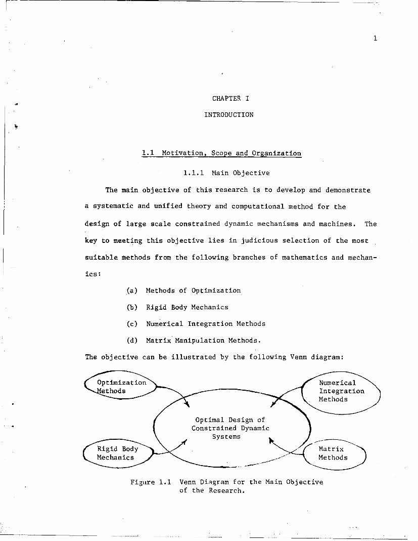
ý0, cost and constraint functionals

G functions in initial conditions

i- , ., VC e functions defining spring-damper variables

X v six times the number of bodies

functions as defined in Eqs. (2.36) and (2.37)

p an integer

v(b),v(b) initial solution variables as functions of b

X Y functions in design parameters constraints

a small number appearing in Eq. (4.6)n

small constant; belong to

local truncation errorC T

I" L 2-Norm

absolute value

(') time derivative

closed interval

<'>,<<->> symbols for definition of special functions

['] denotes reference numbers

* notation for footnote; computer symbol formultiplication

DSIN,DCOS sine and cosine functions with double precision

S=$ definition and equivalence symbols respectively

b (j),z(j) values of the vectors b, z, p, k at the j-th iteration1( ),l(j) • of optimization

xviii

1

CHAPTER I

INTRODUCTION

1.1 Motivation, Scope and Organization

1.1.1 Main Objective

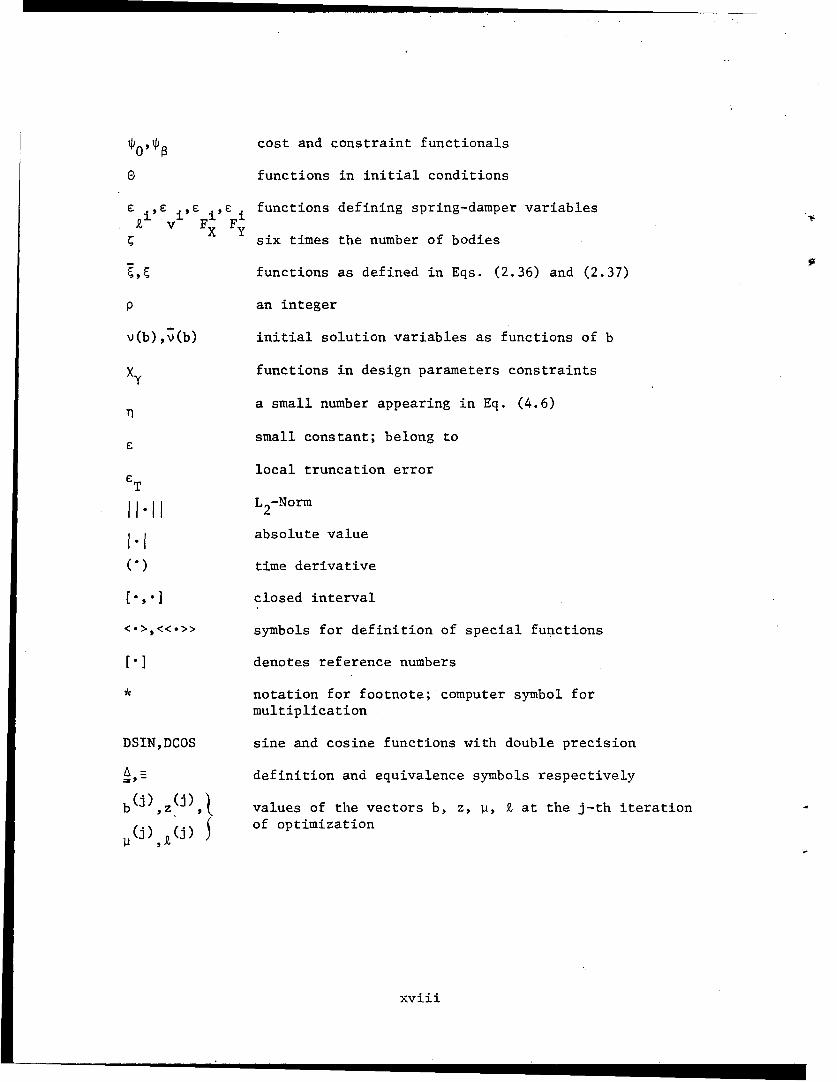
The main objective of this research is to develop and demonstrate

a systematic and unified theory and computational method for the

design of large scale constrained dynamic mechanisms and machines. The

key to meeting this objective lies in judicious selection of the most

suitable methods from the following branches of mathematics and mechan-

ics:

(a) Methods of Optimization

(b) Rigid Body Mechanics

(c) Numerical Integration Methods

(d) Matrix Manipulation Methods.

The objective can be illustrated by the following Venn diagram:

Figure 1.1 Venn Diagram for the Main Objective

of the Research.

2

The arrows on the diagram may be viewed as the process of selecting

from among a large number of alternatives in each area a method that is

compatible with those of the other areas, together providing a qualita-

tively new design capability. Such a comprehensive treatment has never

been attempted, so utmost possible care has been taken in the theoreti-

cal investigation to implement the most suitable computer algorithms

associated with various branches of mechanics and mathematics noted

above. Brief discussions of the above branches, together with the

indication of the methods selected, are given below.

1.1.2 The Notion of Optimal Engineering Design

The job of "optimal engineering design" is to develop the best

possible system for the given application, consistent with resources

allocated to the development phase. Although the notion of optimiza-

tion is inherent in the design process, optimization as a formalized

approach to engineering design is a relatively new concept. It is in

the judicious selection of a "quantitative measure of performance" of

the system and in quantifying performance constraints that an optimal

design is distinguished from a conventional design.

After quantification of the notions of a design process comes the

role of selection of numerical methods for its solution, using the

modern high-speed digital computer. Great strides have been made with

digital computers in the past two decades, to allow for numerical

analysis as a test of an idea or concept, rather than previous cut-and-

try techniques. In this report, advantage is taken of advances in

computer-aided design techniques [1].

3

The field of optimal design of constrained dynamic systems is

of growing interest and importance. In the realm of dynamic mechanisms,

both continuous (smooth) and intermittent (discontinuous) motion-

occurs. For many mechanisms, the logical sequence of events in inter-

mittent motion is known in advance and the total period of motion under

consideration can be divided into intervals of continuous motion. Also,

some intermittent motion can be reduced to continuous motion by the

introduction of artificial spring-damper systems (see Chapter VI).

Thus, derivation of a unified technique for optimal design of dynamic

systems with continuous motion is of major importance.

1.1.3 Methods of Optimization

The fundamental problem of infinite dimensional optimal design

can be described by the problem of Bolza and its extended version that

accounts for inequality functional constraints (see [1]). A corre-

sponding problem for constrained dynamic systems with continuous motion

is formulated in Chapter III. There are many indirect methods [1]

based on a powerful Functional Analysis theorem of Liusternik and

Sobolev [69] for the solution of such problems. But generally they

pose serious computational hazards. In this dissertation a direct

numerical method of solution is adopted.

The basic idea of the direct method of solving optimal design

problems is to first construct an initial estimate of the solution and

then to find small changes in the design parameters such that the modi-

fied design forms an improved-estimate of the optimum, in some sense.

Before design improvements can be determined, analysis of their effect

4

on the problem must be performed. This forms the sensitivity analysis

part of the design process and is of extreme importance.

In the approach used here, design sensitivity analysis uses

state-space methods (see [243) in which the state variables and design

parameters are first treated as independent variables and the elimina-

tion of the variations of the state variables is performed through use

of adjoint differential and algebraic equations (see Chapter III and

references [1,70]).

1.1.4 Rigid Body Mechanics

There are two general approaches to the subject of rigid body

mechanics. They can be called the "Vectorial or Newtonian approach"

and the "Analytical approach". Vectorial dynamics is based on a direct

application of Newton's laws of motion and concentrates on the forces

and motion associated with individual parts of the system, whereas

analytical dynamics is concerned with the system as a whole and uses

descriptive scalar functions such as kinetic and potential energies.

The most direct analytical approach is the well-known Lagrangian for-

mulation. For details, references [66,67,68] are recommended.

In most treatments of optimal design of dynamic systems in the

literature, the number of generalized coordinates of a system is taken

equal to the number of degrees of freedom of the whole system, so that

with the application of Newton's laws, the number of first order ordi-

nary differential equations for thie state is equal to twice the number

of physical degrees of freedom. In general, a dynamic mechanism may

be very complicated and direct application of Newton's laws may result

5

in a highly nonlinear set of differential equations. Moreover, the

eigenvalues for such a nonlinear system may vary over extreme ranges

during the process of numerical integration. Therefore, there remains

a danger of the numerical integration problem turning "stiff" [2,3,4,

4 5,6].

Orlandea [7] and Orlandea, Chace, and Calahan [8] have developed

a node-analogous sparsity-oriented approach to the dynamic analysis of

mechanical systems using the Lagrangian formulation of rigid body

mechanics. By applying SPARSE MATRIX [9,64,65] and STIFF [10] inte-

gration algorithms, large sets of sparse linear equations can be effi-

ciently solved with moderate expenditure of CPU time and the numerical

instability [2,3,6,11] associated with widely split eigenvalues at any

stage can be avoided. Both sparse matrix techniques and stiff inte-

gration algorithms are in the constant process of modification and

refinement. These topics are treated briefly in Chapter II of this

report (also see Sections 1.1.5 and 1.1.6).

These algorithms have been implemented by Orlandea [7] to generate

a computer program "ADAMS" (Automatic Dynamic Analysis of Mechanical

Systems). This program was developed for efficient simulation of

dynamic mechanical systems (e.g., vehicles and machinery) using methods

of numerical analysis developed for electrical circuits [10,12,13].

Orlandea's work has demonstrated that the sparse matrix formulation and

numerical methods involving stiff numerical integration techniques can

be effectively used for simulation of large three-dimensional mechanical

systems. The advantages and disadvantages of these can be stated as

follows:

6

Advantages:

1) No topological preprocessing is necessary to establish a set of

independent variables; equations can be developed directly from

the connection data, component by component.

2) High sparsity of the "Jacobian Matrix" is used in a stiff integra-

tion algorithm (see Chapter II).

3) All angular and displacement variables are retained as solution

variables; none are eliminated in the interest of producing a

reduced set of equations with fewer variables. In this way the

total number of matrix operations and the number of operations

for eliminating variables from nonlinear equations are kept at a

minimum.

4) All joint reaction forces are determined directly in the solution

and therefore the formulation is compatible with current methods

of continuum mechanics for internal stress-analysis.

5) Frictional effects in joints are routinely handled.

Disadvantages:

1) Nodal formulation results in more equations than loop formulation.

2) Some time may be wasted in solving for variables of little interest

to the designer.

ADAMS, IMP (Integrated Mechanism Program) [15,16], and DRAM

(Dynamic Response of Articulated Machineries) [17,18] are the three

main computer programs at present for dynamic simulation of mechanical.

systems. Both DRAM and IMP use relative coordinate systems for parts

(or bodies or nodes) of a mechanism and consider independent loop

7

equations for the determination of constraint equations. These are

complicated mathematical relations involving numerous matrix inversions.

ADAMS, on the other hand, deals with a global inertial reference frame

for all bodies in the system. It will be evident from the formulation

and analytical procedure in Chapters II and III that the ADAMS program

is extremely suitable for optimal design investigations. All the above

mentioned programs, however, use Lagrange's equations of motion in the

analysis.

There are other dynamic analysis programs, namely, IMP-UM (IMP at

the University of Michigan), MEDUSA (Machine Dynamic Universal System

Analyzer) [19], VECNET (Vector Network) [20], and DYMAC (Dynamics of

Machinery) [21]. They deal with different methods of rigid body

dynamics. A more detailed overview of all the programs can be obtained

in reference [22].

It should be noted that, theoretically, any of the dynamic anal-

ysis programs discussed in the foregoing can be used to predict system

dynamics. An apparent advantage inherent in all the programs except

ADAMS lies in the fact that they deal with a minimum number of inde-

pendent (generalized) coordinates and thus involve fewer equations

than does the ADAMS method. The disadvantages of these methods are

much more serious, however. The reduced set of equations with fewer

variables is highly nonlinear. Consequently, the eigenvalues for such

nonlinear systems may vary quite unpredictably during the integration

process. Another major disadvantage lies in the fact that they do not

evaluate the reaction forces simultaneously with the solution variables.

8

In a reasonable optimal design formulation, one generally places bounds

on reaction forces at joints (see ChaptersIll and VI). All these

problem areas are readily handled by the ADAMS modeling method, which

makes the ADAMS method extremely suitable for optimal design investi-

gations.

Wehage [141 has written a program for planar systems using con-

strained system formulation and sparse matrix methods. This program,

after several modifications, has been extended and implemented as the

analysis module of the computer program "DADS" (Dynamic Analysis and

Design System) in this dissertation (see Chapters II, V).

1.1.5 Numerical Integration Methods

The solution of linear dynamic state equations can always be

expressed in analytic forms. But when the equations are nonlinear,

the analytic forms of solutions seldom exist and one is compelled to

resort to graphical [42] or numerical methods. The most serious short-

coming of graphical methods lies in their inapplicability for higher

order, nonlinear mechanical systems. On the other hand, numerical

methods are valid and appropriate for nonlinear systems of any order.

In view of their greater generality and ease of implementation on a

digital computer, numerical methods are widely applied. In the follow-

ing, most discussions will be confined to nonlinear systems. For

detailed analytic theory of numerical methods, references [2,3,4,6,11,

43,44,45] are recommended.

In the Lagrangian formulation of the equations of motion of a

constrained mechanical system, when all the generalized coordinates

9

and Lagrange multipliers are taken to be independent [66,67], nonlinear

algebraic equations enter into the system of equations (see Section 2.1).

As put forward by Gear [46], such a system can be written as:

F(= (1.1)

where y is the solution variable vector, t is the time parameter, and

yis the vector of time derivatives. A member of Eq. (1.1) may be

either a differential or an algebraic equation, according a aF/3y is

nonzero or zero. Such a system of equations is called a simultaneous

system of Differential and Algebraic Equations(DAE's). To the system

of equations (1.1) one must add the appropriate initial conditions of

the form

X() = o (1.2)

where y is a vector of the subset of solution variables having time

derivatives in the system of Eq. (1.1).

Although there exist many algorithms for the solution of initial

value problems, most of them are based on two basic approaches:

(1) the Taylor series expansion approach and (2) polynomial approxi-

mation approach. Algorithms based on the first approach are generally

called Runge-Kutta algorithms and those based on the second one are

usually called numerical integration algorithms (see references [2,6]).

The former are single-step algorithms, whereas the latter are multistep

algorithms that use information from previous time steps. Adams-

Bashforth and Adams-Moulton algorithms are examples of the second

category [2,6].

10

In most of the treatments found in the literature, these algo-

rithms deal with the system of equations of the form

(1.3)

X(O) =o

which do not include algebraic equations. Gear [2,46,48] appears to

be the first person to present a multistep algorithm that deals with

a simultaneous system of differential and algebraic equations, together

with the difficult concepts of stability, convergence and automatic

change of order and step-size (see references [2,6]). Hachtel, et al.

[49] have used this algorithm for electrical network analysis and

design. Calahan and Orlandea [7,8,9] have modified the Gear algorithm

and used it in the ADAMS computer program for the solution of the

dynamic system equations. The Gear algorithm has been used in this

dissertation for the solution of linear and/or nonlinear sets of

differential and algebraic equations (see Chapter II, III and V).

1.1.6 Matrix Methods/

In the process of numerical integration, solution of simultaneous

linear equations is inevitable at every time step. Theoretically, any

method of solution by the L U factorization procedure (see [6,11,44,55])

can be adopted.

By the sparse matrix formulation of the dynamical equations,

difficulties withnonlinearities in the differential equations can be

avoided and so by the application of Gear algorithms and sparse matrix

11

techniques, large dynamic systems can be simulated very effectively.

Thus sparse matrix approaches have been adopted in this dissertation.

Section 2.3 of this dissertation deals briefly with sparse matrix

techniques. Some modifications necessary for the adjoint analysis

(see Chapter III) are noted in that section.

1.1.7 Thesis Organization

In the remaining part of this chapter (i.e., in Section 1.2), a

brief literature survey on optimization of dynamic systems is made.

In Chapter II a sparse matrix formulation of the equations of

dynamical systems and the topics of stiff integration and sparse matrix

techniques are discussed. The formulation of the general optimal de-

sign problem and the corresponding design sensitivity analysis and

optimization algorithms are described in Chapters III and IV.

In the sensitivity analysis, two types of state variables occur.

In mechanical problems, the first type corresponds to variables like

displacements and velocities and are called "Primary" state variables.

The second type corresponds to Lagrange multipliers of the constrained

motion and the spring-damper associated variables. These are termed

"Secondary" state variables (see Chapter II). Chapter V deals with the

organiztion and description of the computer program DADS. Numerical

results of application of this program to slider-crank mechanism and

spring reset plow-share mechanism are presented in Chapter VI.

Finally, some discussion, conclusions and recommendations are given

in Chapter VII.

12

1.2 Literature Survey

A general survey of mechanical design optimization is presented

by Seireg [23]. Haug and Arora [24] have given a description of state

space techniques for solving optimal mechanical design problems. Also

'4a fundamental treatment of the problem of optimal design of constrained

dynamic systems can be found in AMCP 706-192 [l]- Sevin and Pilkey

[25] have used the penalty function technique [26] to obtain min-max

response of dynamic systems with incompletely prescribed input func-

tions. Sevin, Pilkey, and Kalinowski [27i have formulated problems of

optimal design of mechanical systems subjected to dynamic loads in

mathematical programming terms. These can be found in reference [28].

They have studied three types of variational problems: (1) Extreme

disturbance analysis with bounds on performance index for a given

system when the inputs are described as a class of unspecified wave-

forms; (2) optimum system performance dealing with bounding a perfor-

mance index for a class of inputs when certain system elements are

unspecified and constraints are imposed on the system response; and

(3) optimum system design concerning identification of parameters

that uniquely specify the system, so that a performance index is mini-

mized for the worst disturbance among the class of admissible inputs.

For these problems, solution techniques are based on linear, nonlinear,

and dynamic programming [29].

Brock [30], Den Hartog [31], Hamad [32], Arora, Rim, and Kwak [33],

Afimiwala and Mayne [34], Willmart and Fox [35], McMunn [36], and

Kwak [37] have considered various aspects of optimization in vibration

13

absorbers and vehicular models. Hsiao [38] has considered similar

problems with "P-Norm approximation" and/or "Equivalent Functional

Treatment" of cost functional and performance constraints. Haug and

Arora [39] have made further modifications of Hsiao's treatments.

However, all these pr6blems involve either a small number of degrees

of freedom or they are relatively easy to formulate by Newton's laws

(owing to restricted dynamic motions).

In the field of intermittent motion of dynamical systems, very

little work has been done so far. The general problem of optimization

of mechanical systems with this type of motion has been treated in

reference 1. Huang [401 and Huang, Haug, and Andrews (41] have

developed a state-space method of optimal design of mechanical systems

with intermittent motion, which has been applied to a cammed, three

mass system. None of these methods has gone into the consideration of

the problem of instabilities associated with a highly nonlinear set of

differential equations and with widely split eigenvalues. Thus none

has taken advantage of the modern methods of stiff integration (Gear)

and sparse matrix algorithms.

14

CHAPTER II

SPARSE MATRIX FORMULATION OF EQUATIONS OF MOTION,-THE STIFF INTEGRATION (GEAR) ALGORITHM,

AND SPARSE MATRIX TECHNIQUES

2.1 Sparse Matrix Formulation of theMechanical Systems Equations*

2.1.1 Introduction

The principal objective of this section is to present a sparsity-

oriented formulation of dynamical equations using the idea of writing

the equations of motion for each element (or component) of a mechanism

(machine) separately. This idea originated in reference [7] and is

discussed further in reference [8]. In this approach, the Lagrangian

formulation of equations of motion is adopted and constraint equations

for various joints and spring-damper relations are written separately.

No attempt is made to reduce the number of solution variables through

the process of elimination. Thereby, the order of nonlinearity in the

equations is kept at a minimum. The equations are then solved numeri-

cally using a stiff integration algorithm [2,6] and sparse matrix

[9,64,65] techniques. These methods are discussed briefly in Sections

2.2 and 2.3.

The results presented here are confined to two-dimensional mechani-

cal systems. Thus, the. sparse matrix formulation of dynamical

Companion reading of references [7,14,631 is suggested for thereading of this section.

15

equations for such systems is presented here. A similar formulation

for three dimensional systems is available in reference [7].

2.1.2 Two Dimensional Systems

In the Lagrangian formulation [66,67,68] the general form of the

equations of motion can be written (for constrained or unconstrained

systems) as:

d / E E Q. = 0 (2.1)dt kq. j

where

E = Kinetic energy of the system,

q. = generalized coordinates,

ij = generalized velocities,

Q. = generalized forces (conservative or non-conservative

including reactions and spring-damper forces),

j = 1,2,...,k, (where k represents the number of degrees

of freedom),

t = time.

The system of Eq. (2.1) can be equivalently written as

d (I E\ E Q =0 , j = l,...,k (2.2)dt kDiqj

u. j = 0 , j = 1,...,k (2.3)

For constrained systems, the Lagrange multiplier method [66,67]

is adopted and Eqs. (2.2) and (2.3) can be replaced by

16

F .d / aE ý

Fu q Qj + 1j 0 (2.4a)lj d t Faj q. j _~ ýqoJ

F u. - q= 0 j = 1,2,...,k (2.4b)2j j

and

0i = 0 i 1,2,...,p (2.4c)

where Pi are geometrical constraint functions, Q. are generalized

forces (excluding constraint reactions), and pi are Lagrange multi-

pliers.

2.1.2.1 Choice of Coordinates

In two space dimensions, let 0X,0Y represent a set of coordinates

fixed in an inertial reference frame and 0.xi, 0iYi represent a set

of body-fixed rectangular coordinate axes fixed at 0. in the i-th body1

of the system. Let Xi, Yi' ci be the translational and angular gener-alized coordinates and u.i X. vi= Yi, and w =. the corresponding

generalized velocities for the i-th body. These coordinate systems

are illustrated in Figure 2.1. Let

SH[Xi,Yi,4i]1 1 T.

and (2.5)

iiu i [uillvi~w i]

Then, one can write the vector Z i(t) of generalized coordinates and

velocities as

17

YYyy

x .

xxi

Yi

Figure 2.1 Definition of the Generalized Coordinatesfor the i-th Body.

18

.T iT T[u 3 2 ([ui,vi,wi,Xi,Yiti]T (2.6)

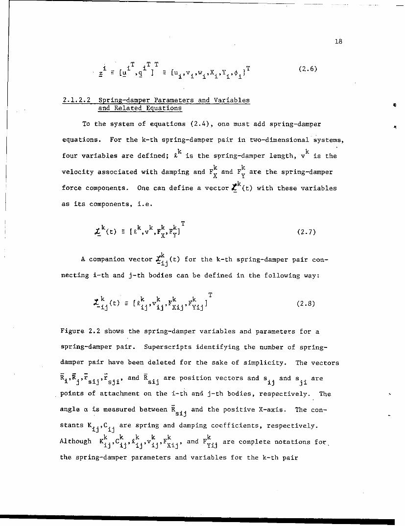
2.1.2.2 Spring-damper Parameters and Variables

and Related Equations

To the system of equations (2.4), one must add spring-damper

equations. For the k-th spring-damper pair in two-dimensional systems,£kk

four variables are defined; k is the spring-damper length, vk is the

velocity associated with damping and F and F are the spring-damperx Y

force components. One can define a vector Zk(t) with these variables

as its components, i.e.

k k k k kFTXk(t) 2 [2 ,v ,F XFy (2.7)

A companion vector . (t) for the k-th spring-damper pair con-

necting i-th and j-th bodies can be defined in the following way:

k (t) k k Fk T (2.8)[ij 'ij' Xij Yij

Figure 2.2 shows the spring-damper variables and parameters for a

spring-damper pair. Superscripts identifying the number of spring-

damper pair have been deleted for the sake of simplicity. The vectors

RiRjrsij,rsji, and Rsij are position vectors and sij and s.. are

points of attachment on the i-th and j-th bodies, respectively. The

angle a is measured between R .. and the positive X-axis. The con-s1J

stants K ij,Cij are spring and damping coefficients, respectively.

k k k k k kAlthough K.ij.,Ci, ij,vij,Fxij, and Fy are complete notations for

the spring-damper parameters and variables for the k-th pair

19

Yx!

rsi i

•jj

Figure 2.2 Variables and Parameters for a

Spring-Damper Combination.

20

connecting the i-th and j-th bodies, superscripts, subscripts, or

both may sometimes be suppressed in the ensuing discussions, for the

sake of notational simplicity.

Explicit defining expressions for the spring-damper variables

are given by (see [14])

k k2 k k 2 ke(U - U + (V- V.) 0 (2.9)

k 3k

C k k _v =0 (2.10)v

K k + 0 ckk

Fx 1

(2.11)

C [Kk (zk _ 1k )+Ck k +Fk IVk Vk 11,k _Fk=0SF •• kv 0 0o~ jv vi/• Yky - K(. L)+Cv+F ] [V V]2 - Fy =0

Y1

(2.12)

k k k kwhere (Ui,Vi) and (Uj,Vj) are the global coordinates of the

points of attachment of the k-th spring-damper pair on bodies i and

J epetvey k an kJ, respectively; K and C are the spring-damper constants; and

k kk0 and F are the initial length and constant force along the spring-0 0

k kk kdamper. The explicit expressions for Ui,Vi,Uj, and V. are given by11JJ

kU.i = Xi +x si3, cos i - Ysij sin i (2.13)

V = Y. + s. sin i + Ysij cos i (2.14)1l 1 51j 1 S1

Uk = X. + x .. cos j - y .. sin Cj (2.15)U. 3i s

J J 5J J ' JI iJ

21

Vk -Y. + x .sin j+ Cos . (2.16)J J s3 i J sj i

where (x sijYsij ) and (x sji,ysji ) are the coordinates of the points

s . and s.i, with respect to their respective body-fixed coordinate

axes.

The functional symbols 6 k,: k'F k'C k in Eqs. (2.9)-(2.12) are. Vk FX Fy

x Y

written to indicate the small values the expressions will take during

Newton iterations in the dynamic analysis (see Section 2.2 and

reference [6]).

2.1.2.3 Constraint Equations

In two dimensions there are two principal types of joints;

revolute and translational. Figure 2.3 shows parameters and

coordinates associated with a revolute joint. In the figure, r isP

the position vector of a point Pji on body j with respect to a point

Pij on body i. When r = 0, P.. and P.. coincide and they define a re-

volute joint. The loop closure relation of the position vectors

gives.

R i + rij + r-r., - R = 0 (2.17)P 1 3J p

Let (xiYi) and (x.,y.)'be the coordinates of Pi. and Pji respectively

with respect to body-fixed axes. With r= 0, the constraint equa-p

tions for a revolute joint between bodies i and j are obtained from

Eq. (2.17) as,

22

C.J

0-

Figure 2.3 Joint Coordinates (r p=0 for revolute joint).

23

DX E X.i + x. cos i -yi sin i -X' -x. cos 4j +y sin •j 0

(2.18)and

ýy Y.+x i sin i+Y. csi-os Y'-x' sin j-y. cos •. = 0

(2.19)

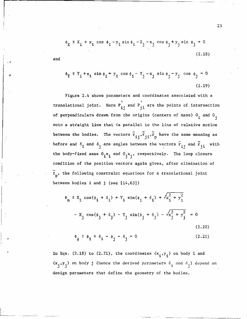
Figure 2.4 shows parameters and coordinates associated with aI I

translational joint. Here P.. and P.. are the points of intersection

of perpendiculars drawn from the origins (centers of mass) 0. and 0.1 J

onto a straight line that is parallel to the line of relative motion

between the bodies. The vectors r. .,ri,rp*have the same meaning as

before and S. and 6. are angles between the vectors r;. and r.. with1 J 1J

the body-fixed axes 0.x. and 0.x., respectively. The loop closure11 JJ

condition of the position vectors again gives, after elimination of

rp, the following constraint equations for a translational joint

between bodies i and j (see [14,63])

n X. cos(•i + 6.) + Y. sin(•i + 6.) + Y2n 1 1 1 1 1 1 1 1

-Xj cos(pj + 6.) - Yj sin(4j + 6.) - 2+ Y 0

(2.20)

SD i +i-. -' = 0 (2.21)

In Eqs. (2.18) to (2.21), the coordinates (xiy.) on body i and

(xj,y.) on body j (hence the derived parameters 6. and 6.) depend on

design parameters that define the geometry of the bodies.

24

7 Xi

pij

line of relativemotion between bodies

Figure 2.4 Translational Joint.

25

2.1.2.4 Primary and Secondary State Variables,Design Parameters

In the problem of optimal design of constrained dynamic systems,

state variables and design parameters are encountered [1]. In the

present formulation, two kinds of state variables are defined:

Primary State Variables: Variables whose time derivatives appear

in the equtions of motion or in related equations are called

"Primary State Variables".T T J J2iT i1

For the planar systems treated here, u ,q , and z ,2 ,...,

3Z k (the last k terms being the lengths of the k spring-damper pairs

connecting i-th body) are Primary State Variables related to the

i-th body.

Secondary State Variables: Variables that appear without their

time derivatives (i.e., appear algebraically only) in the equations of

motion and related equations are called "Secondary State Variables".

Let 4i (t) denote the Lagrange multiplier vector correspond-

ing to the constraints on the i-th body. Then the variables

•iTvj 1 J2 Jk Jl J2 ]k 31 32 Jk

,v ,...,v ,FX ,FX ,...,F Fy ,Fy ,...FY are secondary state

variables related to the i-th body.

The vector b denotes the design parameter vector for the entire

system.

2.1.2.5 Element State Equations of Motion

In the Lagrangian formulation [66,67,68] of the equations of

motion of a two dimensional constrained mechanical system, when all

P. is kept with other spring-damper variables int k(t) for advantagesin computer programming.

26

the generalized coordinates and Lagrange multipliers are taken to

be independent, the state equations of motion for the i-th body of the

system can be written as (cf. Eqs. (2.1) and (2.4)),

i .ipi(b)zi + f. =0 (2.22)

where

Mi 0

iM

pi(b)E J. (2.23)

-1-1

1 0 -1

M. and J. are the mass and moment of inertia of the i-th body,1 1

-if " -i - a • k '' " kk~=SXi k=l i

1 [Q ± k- -- •W

"k k= 1, 2 ,...,pi, are the components of the Lagrange multiplier vector

(t), and Qx.' QY,'Q4 i are generalized forces (including the contri-

butions from spring-dampers). Equation (2.23) indicates that M. and1

J. may be taken as design parameters. Note that the last three equa-1

tions of Eq. (2.22) contain • explicitly. This structure is intro-

duced, intentionally, in order to increase sparsity (see Section 2.3).

27

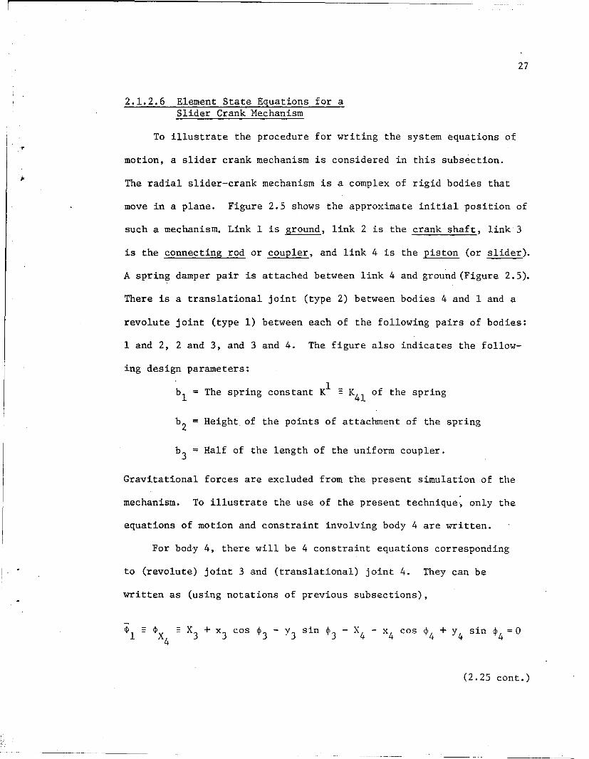
2.1.2.6 Element State Equations for aSlider Crank Mechanism

To illustrate the procedure for writing the system equations of

motion, a slider crank mechanism is considered in this subsection.

The radial slider-crank mechanism is a complex of rigid bodies that

move in a plane. Figure 2.5 shows the approximate initial position of

such a mechanism. Link 1 is ground, link 2 is the crank shaft, link'3

is the connecting rod or coupler, and link 4 is the piston (or slider).

A spring damper pair is attached between link 4 and ground (Figure 2.5).

There is a translational joint (type 2) between bodies 4 and 1 and a

revolute joint (type 1) between each of the following pairs of bodies:

1 and 2, 2 and 3, and 3 and 4. The figure also indicates the follow-

ing design parameters:

bI = The spring constant K 1 K41 of the spring

b2 = Height of the points of attachment of the spring

b3 = Half of the length of the uniform coupler.

Gravitational forces are excluded from the present simulation of the

mechanism. To illustrate the use of the present technique, only the

equations of motion and constraint involving body 4 are written.

For body 4, there will be 4 constraint equations corresponding

to (revolute) joint 3 and (translational) joint 4. They can be

written as (using notations of previous subsections),

1i P X4 3 3 cos 3 -Y 3 sin 3 -X 4 -x 4 Cos 4 + y 4 sin 4 =0

(2.25 cont.)

28

t4-4

__ 0

0- to'

44l

0J

r-4 r

Cc p

29

(D2 0 Y. 3 + x sin 43 + Y Cos 3 - -x sin Co4 - CS os 4 = 04

S2 +24X4 cos( 4 + 64) + Y sin( 4 + 64)Y

3 n4 4 4 4 4 4 4x 4 +

) y2 2XI cos(+5 1 ) -+YI sin(4l + 61) - +Y 0

4 •4 44+64 41 610 (2.25)

The spring-damper relations for the pair connecting bodies 1 and

4 can be written as

kij(U -U4) 1 1 1 =0

CVI

(2.26)

=[KI(k 1 P- 1 )+ C 1 v1 + FI IN u 1 ]/- - F1= 0V 01 1 40

FX

11 1 = 0

F K i - 0 )G 0 1 4 Y

where1

U1 = X1 + xs 1 4 cos 0 1 - Ys1 4 sin i1

1V YI + sin 4l +y cos 4iV1 1 s14 n1 14 1

(2.27)

1 = X + x coss

I = Y4 +x sin 4 + 41s 044 4 Xs41 sY4s41 os

30

(Xsl 4,ysl 4 ), (xs 41 ,ys4) are respectively the coordinates of the points

s14 and s41 of attachment of the spring-damper pair.

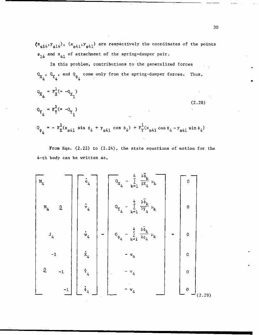
In this problem, contributions to the generalized forces

QX49 QY4' and Q 4 come only from the spring-damper forces. Thus,

Q F(=1 )x 4 x x1Q4 -Q1

(2.28)1

QY4 1QY1

= 1 1

Q F 1(x si + y cs ~)+ F 1(x Co si4 s41 in 4+ s41 c' 4 Y s41 os4-Y 4 1 sinp 4

From Eqs. (2.22) to (2.24), the state equations of motion for. the

4-th body can be written as,

"4 04 x4 k=l 4k4 k i

M 0 Q )Y P 04 V 4 QX4 k=l 44 ak0

-40$ QY k=l • 4-- k 0

-l 4 0~04 4 Q Pký4 k=l $4

-1 4 - 4 0

$4 ( 24 0-- - - (2. 29)

31

The equations of motion and constraint relations for other bodies

of the mechanism can be written in a similar manner. However, manual

formulation of the equations is unnecessary, since the computer program

ADAMS-2D [14] automatically generates the necessary code for all the

expressions and equations. Only data defining parameters such as

mass, moments of inertia, locations of centers of mass, location of

joints and points of attachment of spring-damper pairs, and spring-

damper constants, (see [14,63]) are to be provided by the user.

2.1.2.7 Goblal System Equations

For a mechanical system of n bodies, m joints, and s spring-

dampers, the global vector of generalized coordinates and velocities

may be denoted by z, having components zlZ 2,... ,z, where C = 6n.

Z [I1T z2 T , nT]T

nT1

[zlZ 2 ,...,z•]T (2.30)

The global vector of Lagrange multipliers may be denoted by v which,

with its components i is

[Pl, •2' ... 12m-l,'12m] (2.31)

The global vector of spring-damper variables may be denoted by Z;

which with its components £i,£2,2 ... ,.is given by

1 ,m ] ... • 1T (2.32)

32

Now the state equations of motion for the entire system can be

written in the form (deleting for simplicity the underlines of the

vector variables)

F(t,z,z,Z,p,b) E P(b)z + f(t,z,P,,p, b) - 0 (2.33)

where

-P1 (b) 0-

P(b) p2b(b) (2.34)L "~ pn(jn) 6n

- "(6n x 6n)

f 1 f 2 , . . . .if

From equations (2.18) to (2.21) one may summarize the constraint

equations in the form

O(z,b) = 0 (2.35)

From equations (2.9) to (2.12), one may write the equations

related to spring-damper pairs as

- Ii + E(z,k,b) = 0 (2.36)

where

""eE ...[ C I (2.37)i h ebricFX Fy an Y is

Sis the algebraic part of T, and 1 is defined as

33

0 0 01 0

0

0

0 0 (2.38)

1 0

0

0 0

(4s x 4s)

The system of equations (2.33), (2.35), and (2.36) is solved by

Gear's predictor-corrector algorithm and sparse matrix techniques

discussed briefly in Sections 2.2 and 2.3.

2.2 Stiff Integration (Gear) Algorithm

2.2.1 Introduction

Any system of differential equations that has widely split

eigenvalues, at least locally, is called a stiff system. If a

nonlinear system N is apprbximated by a linear system L around some

point t, the eigenvalues of L are'the local eigenvalues of N at t

with respect to L. The mechanical system of Fig. 2.6 represents a

stiff mechanical system. As indicated in Chapter I, mechanical

systems like the ones discussed in Chapter VI may not be stiff ini-

tially, but they may unpredictably become stiff. It has been shown

in references [2,6] that neither Runge-Kutta nor Adams-Bashforth

nor Adams-Moulton algorithms are suitable for the solutions of such

systems, for stability reasons [2,6].

34

u

W)

5-4C0 CD C

CD -ý CD

o( on 0 4 -

-CDt II I0C0D

4- *f U) U 1

I-IJ

cJu

o 0

35

In 1969, Gear developed stiffly stable [2,6,47,48] multistep

algorithms, which are well suited for the solution of stiff systems.

Originally he considered systems of the form of Eq. (1.3) and employed

his criteria of stiff stability to derive the algorithm. Later he

showed [46] that the same algorithm can be used for mixed systems of

differential and algebraic equations. One must understand the techni-

cal details of the subject of multistep numerical predictor-corrector

algorithms and the concepts of stability and convergence and automatic

change of order and step-size in order to have proper command of the

Gear algorithms and their implementation in computer program DIFSUB

(see [7]). These are, however, availabe in standard references [2,6],

and will not be treated here. The basic idea of automatic control of

order and step size can be stated briefly as follows:

Let t.= t represent the current time instant and h and k be then

current step size and order of the numerical integration. Let ST be

the local truncation error [6] and emax the maximum allowable ET'

The basic step control algorithm is then to execute one step and

test whether the relation

ET < Emax (2.39)

is satisfied. If it is, the step is accepted. Otherwise, the step

is rejected and a smaller step size h = h(a < 1) is used. The

exact step size to use for executing the next step, or for repeating

the rejected step, is given by the choice of a as the maximum value

computed from three expressions [6] for local truncation errors

36

corresponding to the orders k, k - 1, and k + 1. The maximum of the.

three a's gives the maximum allowable step size and the corresponding

order is the optimum order to compute values at t = t ..n+l*

2.2.2 The Gear Algorithm and the Mixed Systemof Differential and Algebraic Equations

The k-th order Gear algorithm for the solution of the mixed

system of differential and algebraic equations (1.1) and (1.2) is an

implicit algorithm of the form

Xn+l - 0 h jn+l - (a0 y n +a lyn- 1 + + ck-lYn-k+l)

k-l0 h yn 1 - a.j n-j (2.40)

where h is the time step, yn+l'Xn,... are the values of y at time

instants t n+l,t and a0,1k,...,ak-l,80 are the (k + 1) coeffi-.

cients known as Gear coefficients for this multistep algorithm [2,6].

One proceeds from the nth to the (n + 1)st time step by solving

Eq. (2.40), together with Eq. (1.1) at t = tn+l, i.e.

E6 n+l',n+l' tn+I) = 0 (2.41)

Linearization of Eq. (2.41) gives the Newton formula [6] at the

(n + 1)St time step:

3 F(m) aF(m)_____ (m) + -- AY(m) -F(m) (2.42)

AA + Ay

4

37

where

AX(M) (mr+l) y (M)

(2.43)

A(m) ff(m+l) -(m)

m being the iteration number in the Newton method of solving the

algebraic equations. The time step counter n has been dropped, for

simplicity of notation.

k-iSince I a Jyn-j remains invariant for Newton's iteration at

j0•

the (n + 1)st time step, one obtains from Eq. (2.40)

A~y(m).= -a 0h Aýy(M)

or (2.44)

A (m) 10- A_(M)

Hence, Eq.' (2.42) becomes (after the substitution of the second of

Eqs. (2.44))

[)F (M) 1 F(m)

h AZF (2.45)_ _ 1 oh(in) - Fm

This is called the "corrector formula" for y at the (n + 1)st time

step.

Equation (2.45) 'together with the second equation of Eq. (2.44),

updates both y and y, which are required in F(m). The iteration is

continued until the right-hand side of Eq. (2.45) is less than a pre-

assigned small quantity. Since the Jacobian matrix on the left-hand

38

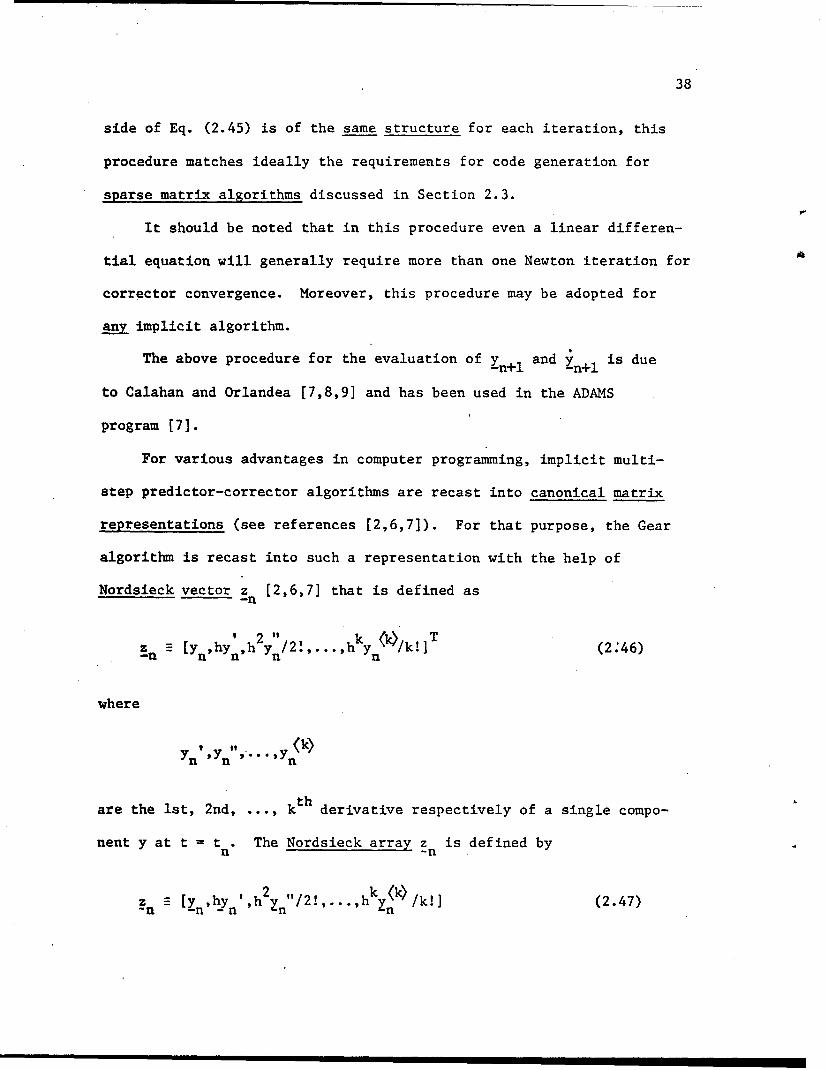
side of Eq. (2.45) is of the same structure for each iteration, this

procedure matches ideally the requirements for code generation for

sparse matrix algorithms discussed in Section 2.3.

It should be noted that in this procedure even a linear differen-

tial equation will generally require more than one Newton iteration for

corrector convergence. Moreover, this procedure may be adopted for

any implicit algorithm.

The above procedure for the evaluation of yn+1 and n+l is due

to Calahan and Orlandea [7,8,9] and has been used in the ADAMS

program [7].

For various advantages in computer programming, implicit multi-

step predictor-corrector algorithms are recast into canonical matrix

representations (see references [2,6,7]). For that purpose, the Gear

algorithm is recast into such a representation with the help of

Nordsieck vector z (2,6,7] that is defined as-n

' 2 k (k) ]TYn .. ,hy n/k! (2:46)

where

,k)Yn 'Yn ''Yn

kthare the Ist, 2nd, ... , derivative respectively of a single compo-

nent y at t = t . The Nordsieck array z is defined byn ~n

z y ,hy ',h 2 xn"/2!,...,hk <k)/k!] (2.47)a -n -n n

39

All the updated values of the Nordsieck vectors are required for pre-

diction of the solution variables that are used as initial estimates in

the corrector iterations. It should be noted here that Eqs. (2.44) and

(2.45) give only the first two components of the Nordsieck vectors.

Orlandea [7] has shown that all the components of the Nordsieck

vectors can be obtained from the corrector iteration formulas of the

form:

[LF(m) i 3F(m) 1 (m)<i) c zi (m),- -- 3j L = Z1- (2.48)

L _ - 0h ax -cz -

where the time step counter n has again been suppressed for simplicity,(m)(i)

the vector z represents the vector of the i-th components of zm -n

at the m-th Newton iteration, and czi, i = 1,2,...,k+l, are the

coefficients of the transformed Gear algorithm. Their values are

given in Table 2.1 (see reference [6]).

The present form of DIFSUB, however, does not iterate for the

values of the Nordsieck vector components other than the first two.

They are evaluated from Eq. (2.48) after corrector convergence for

the first two components.

2.2.3 Starting of Multistep Algorithms

Multistep numerical algorithms are not self starting. Generally

a single step algorithm is used at least k times before a multistep

algorithm can be initiated.

In the ADAMS program, The Gear algorithm is implemented through

the subroutine DIFSUB and initially the order is taken to be 1. The

40

Table 2.1

Coefficients of Stiffly Stable Methodsin Canonical Form

k 2 3 4 5 6

2 6 25 120 720CZ1 3 11 5-- 27-4 1764

3 ii 50 274 1764Cz 2 T 50 27-4 1764

1 6 35 225 1624C 3 3 11- 50 274- 1764

1 10 85 735Cz 4 11 50 27-4 1764

1 15 175Cz 5 5T 27-4_ 1764

1 21Cz 6 27-4 1764

Cz 7 1764

first order Gear algorithm, being exactly the backward Euler algorithm,

is itself a single step algorithm that serves the purpose of initial-

ization.

2.2.4 Corrector Formulas for the Dynamical

System Equations

For the state equations of motion gi-en by Eqs. (2.33), together

with the constraint equations (2.35) and the spring-damper relations

41

(2.36), the corrector formula (2.45) can be written as (deleting

underlines and superscripts),

1 + f af. __-O-- P(b) +-fz pf z

30 0 0 0 -Dz

L - 0h a J L JL J

(2.49)

where the following relations have been used:

aF - f -z

Bz z 9 z

--- --- , D (2.50)

aF af

Moreover, when z [XiYiiuiviw instead of

T[ui vi,wi,Xi,Yi,•i] , one obtains (see Eq. (2.24)),

(- az (2.51)

In that special case, Eq. (2.49) can be written as

42

1af ~ T fZP P(b) + (" fAz F- o---i -•\azj a- P,0I

az 0 0 Ali

az A

0 + A0

(2.52)

A descriptive tableau form for the corrector formula of Eq. (2.49) canbe given as

Iconstraint I spring- IAu1- -FIrelated aAq'j,sparse related Au2

I- submatrices submatrices -2)0Bdy with elements with elements '- '

)T DFof of D- -

---------------- f---- ---constraint related I

sparse submatrices with 0 Al

elements of 8__-aq -

spring-damper related submatrices of the form:

Ak3u ' aq ' at

(2.53)

The matrix in the left-hand side of this corrector formula is

known as the corrector Jacobian matrix. A detailed description of

the nonzero positions in the Jacobian matrix of such a tableau for

the four-bar slider-crank mechanism of Fig. 2.5 is given by Fig. 2.7.

43

2 3

• 4

667 Co,8 E Q

_ _ _ F DFPRC 0

E B G

H U ;7

N K0 L I .

R a AL ID tS21Z 08N CET

__ X ,UY V86 90

78 ABG C H K .1,IJ MN

W X 1 2G YZ 34•

SGH _____ _ CD_

OPQ RST UI vwex Y 2 3 690

ZI 45 1 79 A

Figure 2.7 Symbolic Listing of the NonzeroEntries in the Jacobian Matrixfor the Example Slider-CrankMechanism.

44

2.3 Sparse Matrix Techniques

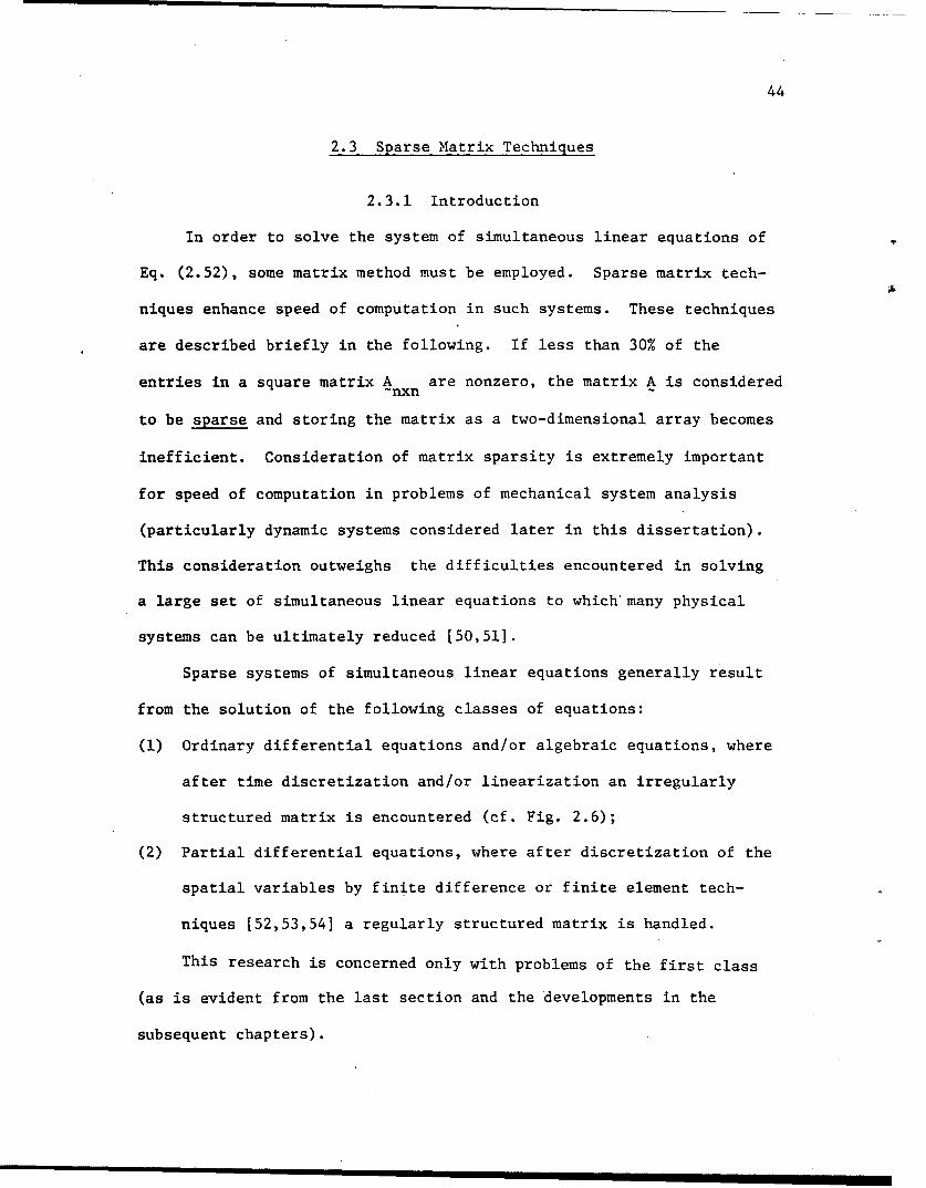
2.3.1 Introduction

In order to solve the system of simultaneous linear equations of

Eq. (2.52), some matrix method must be employed. Sparse matrix tech-

niques enhance speed of computation in such systems. These techniques

are described briefly in the following. If less than 30% of the

entries in a square matrix A are nonzero, the matrix A is considered-nxn~

to be sparse and storing the matrix as a two-dimensional array becomes

inefficient. Consideration of matrix sparsity is extremely important

for speed of computation in problems of mechanical system analysis

(particularly dynamic systems considered later in this dissertation).

This consideration outweighs the difficulties encountered in solving

a large set of simultaneous linear equations to which' many physical

systems can be ultimately reduced [50,51].

Sparse systems of simultaneous linear equations generally result

from the solution of the following classes of equations:

(1) Ordinary differential equations and/or algebraic equations, where

after time discretization and/or linearization an irregularly

structured matrix is encountered (cf. Fig. 2.6);

(2) Partial differential equations, where after discretization of the

spatial variables by finite difference or finite element tech-

niques [52,53,54] a regularly structured matrix is handled.

This research is concerned only with problems of the first class

(as is evident from the last section and the developments in the

subsequent chapters).

45

In sparse matrix methods, operations involving zeros are avoided

by using structural information (the positions of nonzero entries)

that is stored in a compacted form. One way of doing this is to store

the row and column indices of each nonzero element in two vectors I

and J and the value of the elements in a third vector G. This method

is called "i-j" ordering. According to Calahan [10] this is the most

convenient method and can be easily converted to other methods of

compacting the data, such as the threaded list method and the bit map

method, which are discussed in detail in [10].

2.3.2 Solution of Simultaneous LinearAlgebraic Equations

There are two general methods for solving a set of simultaneous

linear algebraic equations

B (2.54)

These are (1) the Gaussian elimination method and

(2) L U factorization method [6,11,44]. Although theoretically they

are somewhat interconnected, the solution techniques involve two

different algorithms. The L U factorization method is preferable for

sparse matrix techniques. Since the inverse of a sparse matrix may

be full, whereas L U factors may retain sparsity [10], the number of

operations in the first method is much larger than that in the second

[6]. The method of L U factorization is now briefly described.

46

Let L and U be of the form:

i 0 i...u11~lj in

* . o .iL= 91 **. in

9ni nn

(2.55)

Then to get

A= L U (2.56)

one has with a.. as the elements of A,1J

j-i

Z.ij a.ij - 9 £ik Ukj i > j (2.57)k=1

and

u..j = ij - k 1ik ukj ii i < j (2.58)

which determine the matrices L and U for the matrix A(n xn)"

This method is employed in the Crout algorithm [55] for L, U factor-

ization.

After L U factorization of A, the solution of Eq. (2.54) is

obtained as follows:

L U x = B (2.59)

47

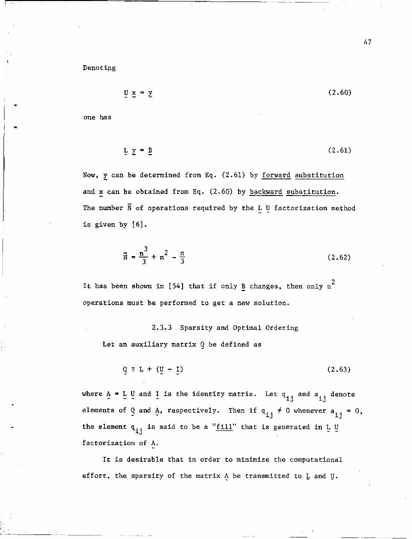
Denoting

U x y (2.60)

one has

L y B (2.61)

Now, y can be determined from Eq. (2.61) by forward substitution

and x can be obtained from Eq. (2.60) by backward substitution.

The number N of operations required by the L U factorization method

is given by [6].

33 2 n-- +n -+ (2.62)33

2It has been shown in [54] that if only B changes, then only n

operations must be performed to get a new solution.

2.3.3 Sparsity and Optimal Ordering

Let an auxiliary matrix Q be defined as

Q = L + (U - I) (2.63)

where A = L U and I is the identity matrix. Let qij and ai. denote

elements of Q and A, respectively. Then if qij # 0 whenever aij = 0,

the element qij is said to be a "fill" that is generated in L U

factorization of A.

It is desirable that in order to minimize the computational

effort, the sparsity of the matrix A be transmitted to L and U.

48

That is, the number of fills should be kept to a minimum. This can be

done by a suitable permutation of rows and columns. Such an operation

is known as Optimal Ordering (or pivoting). Some simple examples

demonstrating the effectiveness of such ordering can be found in [6,7].

Over and above the solution efficiency and the minimization of the

size of the generated code, there is another important reason for

optimal ordering. Most of the equations in physical problems are

nonlinear and the entries in the matrix vary from step to step of a

solution process. In such cases optimal ordering prevents generation

of zero-valued pivots and costly regeneration of the solution code.

The detailed discussions of the subject of optimal ordering is

beyond the scope of this dissertation. They can be found in refer-

ences [56,57,58,59]. Codes such as OPTORD [60,49] and MOOP [61] are

two of several computer programs that can be used for optimal ordering.

Although optimal ordering aims at the largest (absolute value) non--

zero, row-column entry as the pivot and minimization of the number of

fills, generally both cannot be achieved simultaneously and the

algorithm chooses from among the larger than average pivots, the

one which results in the minimum number of fills. The mode of

operation for optimal ordering can be visualized from the following

considerations.

Let K be an integer between I and n that represents the Kth

step associated with the permutation and L U factorization of the

remaining matrix at that pivot step. Every nonzero element in the

residual submatrix of dimension (n - K + 1) is considered as a

49

candidate for the pivotal element. Associated with each nonzero

element A(I,J) in the submatrix is a weighting function:

W(I,J) = (LROWI - 1) (LCOLJ - 1)

where LROWI is the number of nonzero elements in the row containing

A(I,J) and LCOLJ is the number of nonzero elements in the column con-

taining A(I,J). The term W(I,J) represents the number of multiplica-

tions required if A(I,J) were selected as pivotal element. For each

row with I fixed, W(I,J) is determined only for elements that are

numerically acceptable; i.e., if

IA(I,J)l > E - AVG(1)

where 0 < c < lis a user-specified tolerance,

NI

AVG(I) = Y IA(I,J) INI J=l

and NI is the number of nonzero elements in row I. The algorithm

attempts, in a systematic manner, to locate the element with the

largest absolute value and the smallest value for the weighting

function.

2.3.4 Column Ordering of a Matrix

It has been mentioned in Subsection 2.3.1 that the nonzero

values of the original matrix are stored in a vector G. They can be

stored either in row-wise order, taking one row after another, or in

column-wise order, taking one column after another. The optimal

50

ordering algorithms can handle both representations. However, the

subroutines VMSP, VMNP, and VMBP, used in ADAMS programs for L U

factorization of matrices and numerical solution of linear equations,

consider only the column order representation. The various aspects

of all these subroutines are discussed in reference (62]. Many other

subroutines performing similar functions can be found in [61].

In the original arbitrary "i-j" ordering, the row and column

indices are stored in vectors NPOSR and NPOSC, respectively, and the

nonzero elements of the matrix A are stored in the vector G. To

transform the "i-j" ordering into column ordering, a permutation

vector is generated to cause the elements a.. of A to be entered into

the appropriate locations in the vector G.

The process of converting the code from "i-j" ordering to column

ordering is illustrated in Table 2.2. A unique number NRANK(1) is

assigned to each of the NG nonzero entries in the matrix, in such a

way that NRANK increases as one proceeds down a column. No value of

NRANK for a certain column is greater than that for any other column

to its right. After the initialization of a counter NCOUNT in Step 2

and reordering the NRANK and NCOUNT in Step 3, Step 4 generates the

row indices IA(I) of the desired column ordered matrix and Step 5

generates the points JA(I) to the subscripts of the indices of the

first element in each column. Step 6 generates the permutation vector

NPOS for column ordering of the original G vector. This algorithm is

implemented in subroutine S08000 of ADAMS 2-D [14] and SEP of ADAMS

3-D [7]. Simple numerical examples of this procedure can be found in

reference [63].

51

Table 2.2

Column Ordering of a Random Matrix

N = dimensions of matrix

Step 1. Calculate the rank of each nonzero entry:

NRANK(I) = NPOSR(I) + (N +l)*NPOSC(I), I=l,NG

Step 2. Initialize a vector NCOUNT(I) = I, I=l,NG

Step 3. Reorder NRANK from the smallest to the largest.

Reorder NCOUNT along with NRANK

Step 4. Generate a vector IA(I), I=I,NG, that gives the

row indices of the permuted.G vector:

IA(1) = NRANK(I) - (NRANK(I)/(N+I))*(N+l)

Step 5. Generate a vector JA(J), J=I,N, that points to

the index I of IA(I) of the first nonzero entry

in each column, and JA(N+l) = NG +1.

Step 6. Generate a vector NPOS(NCOUNT(I)) = I, I=l,NG.

52

In practice, one makes the assignments G(NPOS(I)) = aij to put

G(I) in column order. The vector NPOS is generated only once and is

never modified during the execution of the program. With the help of

this vector, any element of G can be directly accessed and modified,

if desired.

In the sensitivity analysis (see Chapter III of this report),

the solution of adjoint equations requires column order representation

of the transpose of the original matrix. To achieve this the original

vectors NPOSR and NPOSC are stored in another set of vectors NPOSCI

and NPOSRl, respectively, and subroutine S08000 is called to generate

the vectors NPOS and JPI corresponding to original vectors NPOS and JA.

This is done in subroutine DYNANL (see Chapter V).

2.3.5 Matrix Vectorization

Consider a column of a sparse matrix having the nonzero row

positions shown in Fig. 2.8. This structure is described in the

rth column

2526 (25,28)2728

32 -32

3536 (35,38)3738

Figure 2.8 Matrix Vectorization.

53

conventional ordered list as

25, 26, 27, 28, 32, 35, 36, 37, 38 (2.64)

A list enumerating all the row positions in the column is called

"scalar storage". For large matrices, additional savings in computer

memory and execution time can be realized by further compacting the

column-ordered code. This is done by a subroutine VECTOR after the

optimal ordering operation. The algorithm obeys the following rules.

If in a given column, there is a set of two or more contiguous

row positions, only the first and last row indices are retained in the

vector IA of Table 2.2. This implies that all elements in between

them, the boundary terms inclusive, are nonzero.

On the other hand, if there is an isolated element in a column,

with no nonzero adjacent term, its row index is set negative.

JA of Table 2.2 .is updated to reflect the changes in IA and has

the same meaning.th

Thus after vectorization, the r column shown in Fig. 2.8 is

described in the ordered list as

25, 28, -32, 35,38 (2.65)

Given the vectorized and permuted description of the nonsingular

matrix, subroutine VMSP (Vectorized Matrix Symbolic Preprocessor) can

be used to generate a symbolic description of the L and U matrices.

The numerical L U factorization is performed by subroutine VNNP

(using the code generated by VMSP). Subroutine VMBP then solves the

54

equations by forward and back substitution steps. Upon return from

VMBP, the resultant solution vector is stored in the original

right-hand side vector B of ,the equations A x = B. For further

discussion, reference [62] is recommended.

55

CHAPTER III

FORMULATION OF THE OPTIMAL DESIGN PROBLEMAND SENSITIVITY ANALYSIS

3.1 Introduction

For constrained dynamic systems with just a few degrees of

freedom, the treatment of the optimal design problem given in

reference 1, in conjunction with the Newtonian equations of

motion may be quite sufficient. However, for large systems,

owing to nonlinearity in the system equations, the Newtonian

approach is not convenient. On the other hand, it will be evi-

dent from the next sections that the Lagrangian sparse-matrix

formulation of the equations of motion and implementation of a

STIFF (GEAR) integration algorithm are extremely advantageous.

In the following, discussions will be confined to two dimen-

sional systems. However,their extension to three-dimensional

systems is quite straightforward, at least theoretically.

3.2 Formulation of the Optimal Design Problem

The optimal design problem for a mechanical system of n bodies,

m joints, and s spring-dampers in the notation of Chapter 2 can now

be stated as follows: Determine be R., p being a positive integer,

to minimize the cost functional

56

0= g 0 (bz(O),i(O),Z(tl),z(t 1 ))

ti

+ o 0 [tz(t) ,i(t), (t),b~dt (3.1)

where

Z = 9,i+4j I j=O11l,...,I(s- I)] T, ]T

S[sz 5'''" £(4s-3)] (3.2)

subject to the following conditions:

(a) state equations of motion of Eq. (2.33):

F(t,i,z,,p,b) ---P(b)i + f(t,z,Z,p,b) = 0;

(b) constraints of Eq. (2.35):

(D (z,b) = 0 , a=1,2,...,2m; (3.3)

(c) the equations related to spring-damper pairs (Eq. (2.36));

(d) initial conditions( z(0) - v(b) 0 (3.4)(E (0) - v(b) 0 (3.5)

(e). functional equality constraints

9 (b'z(O),i(0)'z(tl )J(t 1 ))

+ f LEt,zt(t),U (t),b]dt = 0 , $=1,...,r';

(3.6)

and/or functional inequality constraints

•8=g(b' z(0) 'i(0) 'z(t)'it)

+ f 1L,[t,z(t),,(t),Z(t),b]dt < 0 , =r'+l,...,r;

(3.7)

(f) design parameter constraints

57

xy(t,b) = 0, 0 < t < tI , Y =1,2, q'

xy(t,b) < 0, 0 < t < tI , y =q'+ q (3.8)

(g) point-wise constraints of the form

H(t,z,p,2,b) < 0 , 0 < t < tI. (3.9)

The point-wise constraints are transformed to the equivalent func-

tional form of Eq. (3.6) [39]:1l H2 [l+sgn H]dt = 0 (3.10)

or

< H> dt = 0 (3.11)

where 2(H2 , H > 0

< H> = (3.12)

3.3 Sensitivity Analysis

Before developing an optimization algorithm, it is necessary

to determine how changes in design parameters change the cost

functional *09 the constraint functionals ý,' and the constraint

functions XY" From Eq. (3.8), it is clear that the first varia-

tions in X can easily be expressed in terms of 6b. From Eqs.

(3.1) and (3.6) or (3.7), it is seen that 0and d have the same

form, so typical *, g, and L are considered.

Taking the first variation of a typical functional 4, in terms

of all of its variables, one obtains:

58

-g 6b + 9g' z(0) + 3g 6Z(0) + ' 6z(ab z(0) 31(0) az(t 1) )

+ + z+ +3ý6 z)LOd

(3.13)

The first variations of Eqs. (3.4) and (3.5) give:

Sz(O) - ab 6b = 0

(3.14)

am(o) IT 6b = 0

To express 6p solely in terms of 6b, an adjoint variable

X(t) - ,X,,] is introduced through the identities [1,70]

obtained from Eqs. (2.33), (2.35) and (2.36):

T [P(b) +f(t,z,p,Z,b)] = 0 (3.15)

TT O(z,b) = 0 (3.16)

,T 2 +E(z,Z,b)] = 0 (3.17)

where

S(X '1P 2 •6 n )T

x = (X6n+l,...,X6n+2m)T (3.18)(318X' (X 6n+2m+l,'...' 6n+2mI4s) T

Integrating Eqs. (3.15), (3.16), and (3.17) from 0 to tl, one

obtains 0t ýT[P(b)i+f(t,z,£,pb)]dt = 0 (3.19)

fJ.T c(z,b)dt = 0 (3.20)

59

and

tX T[f i+E(z,Z,b)]dt = 0 (3.21)

Integrating the first term in Eq. (3.19) by parts, one gets

TP (b)zt1 Jo' [l T P(b)z _T f(t,z,Z,P,b)]dt = 010

(3.22)

Similarly, integrating the first term in ýq. (3.21) by parts, one

gets

,T 1 Zi _ ,1 (z,t , b)]dt = 0 (3.23)

0

The first variations of Eqs. (3.22), (3.20), and (3.23) lead to

- + a(P(b)z) -Tf l r 1 rf(P(b)z)

- I f6b~d + 0~) z3.24

A L a b 1 0 - [b

+ P(b)6 TT If f6z T If 6PT ýf 6Z

x T af 6b dt =0 (3.24)

>L az z+b 6 b dt = 0 (3.25)

andX, T• z -ttT VT 69E1 X'T I [k

X-I ý b dt = 0 (3.26)

Integrating the first term under the integral in Eq. (3.24)

by parts and making necessary adjustments, one has

TTtl. t - -- Ta(PbP)6

P(b)6z -ftpb(b) 6 b

TT Tf S TTf S T lf -T ff 6-_ T - 6b dt = 0 (3.27)

60

It is to be noted here that in the second term under the integral

of Eq. (3.27) the differentiation is of P(b) only with respect to

b and -f should not be substituted for P(b)i, i.e.,

if P(b)! = Pij (b)ij , j summed,

S(P(b) ) Sb = P i 6bk j$ k summed,

3b ij,k i k

wherea P (b)

P (3.28)ij,k 3bk

It is further noted that 6z(0) and ST(0) are expressed in terms

of 6b by the Eq. (3.14).

Now to express the 4th and 5th terms of the right-hand side of

Eq. (3.13) in terms of 6b, the following boundary conditions are

introduced:

xT (t)= az P(b)1 z(t 1)

and (3.29)

X (t g j=O9l,2, , 1(s-l)2+4j 1t) = (t1) ' l "'"

az1+4j

.. Then, with Eqs. (3.14) and (3.29), Eqs. (3.27) and (3.26) can be

rewritten as

XT (0) P(b) L- 6b -( 6z(t) + LX TP(b)Sz-T 3(P(b)i) 6b - TT If _ TIf

TT- f6t - TT a b at =0 (3.30)

and s-i. 0 s-i s-iV.1,(0) 69 (0) _ 1 x'(O)! b s ag 6z(ti)

I X2+4j 1+4j j0 2+4j 3b (tl) l+4jJ=0 =O j =0 t £1+4j

-~[ý'T(1)- XT 3ý 6z - XT 3 - I'T -b dt

(3.31)

61

Now let A, Tand V' satisfy the adjoint equations

F -P+--T ++ ?= + 'D 0 (3.32)d-t az az az az

' fT - LT 0 (3.33)

aip a la

and

- dXt' afT - + aj X _ aLT 0 , (3.34)

+T at a 1 at-

with initial conditions (3.29) already chosen. With Eqs. (3.32),

(3.33), and (3.34), one obtains from Eq. (3.30)

T(o) (b) a 6b - z(tT ,TA () 3b az(t ) Izt1 3JL~ z+ T

3L aL T 6 z+,T 6 3L6-76z-•- i' .,T •••-

-T a(p(b)£) -T 3f (

6b - -.. •6b dt= 0 (3.35)

Hence from Eqs. (3.25), (3.31), and (3.35), one obtains,s-i avl~

!T(0) P(b) "J 6b +s X' (0) Ig -Z(t)3b0 2+4j 3b az(t 1 )

s- g 6Y(t) + F [ z-1 -1 6

j=03 ~j 1) +4j JLkaz all atj= a91(tl) J 1=031+4j

=T aD ,r 3E -T a (P(b)£) 8b-b 6b - X 6b - 3b 6

-T f 6b dt - 0 (3.36)

Therefore,

ag 6z(t 1 ) + ag 6(t 1 ) + +L [ +-- 9+"- taz(tI a1(t 13 )11 a

TT (0) P(b) " 6b + s A'

j=0 2+4j abt_ -0• (pb)ý) -T 3f b 3,T•

IT IT (P( 6b+X b+ ' 6D+X b t

(3.37)

62

Eq. (3.37) can now be used to eliminate explicit dependence

of 6ý on 6 z, 6p, and 6k and the steepest descent programming meth-

od can be used to carry out sensitivity analysis and iterative

optimization. Substituting from Eq. (3.37) into Eq. (3.13), one

obtains

1& 6$b-+ + fT(o) P(b) av 6b

3- b + (0) 13

+A (+6b+ 7T (p(b)Y)bI j0 24lbL3

XT T X

- 6b dt (3.38)

b b 3bJ

As stated previously, Eq. (3.38) can be applied to all wrt

0 For convenience, define

T agB . T ] • s-i agB

I j = 1 9b"9L T i) l+4j

,•8 ~ ~ ~ ~ _ (O] +tF_8 •B (P (b) ) BT -f

+ 2+4 j • ab(0 F0 3b D"b

s T( and (4 nw pdt (3.39)

which is the design sensitivity coefficient vector of ýa with res-

pect to the design parameter b. With Eq. (3.39), one can write

60= Z*0T6 b (3.40)

andT

6ýB = ZýB 6b , fl1,2,...,r (3.41)

Eqs. (3.40) and (3.41) now provide %0 and 6ý solely in terms of

6b. The generalized steepest descent or gradient projection method

63

of (1] may now be applied to carry out constrained sensitivity

analysis and iterative optimal design.

3.4 Comparison of the Corrector Equations for theEquations of Motion and the Adjoint Equations

For system Eqs. (2.33), (2,35), and (2.36), the corrector

equation can be written (see Chapter II) as:

1 P(M) +af af _f

- h ao - - at F

0 L0

az!

0 0 AtJ

LJ h (3.42)

In a similar manner, the corrector equations for the adjoint

Eqs. (3.32), (3.33), and (3.34) can be written as:

1 + T T T AFB h a az \azj(Z

Taf 0 0 Ax

af T 0 T T Ax-0-h- (3.43)

where the following relations have been used:

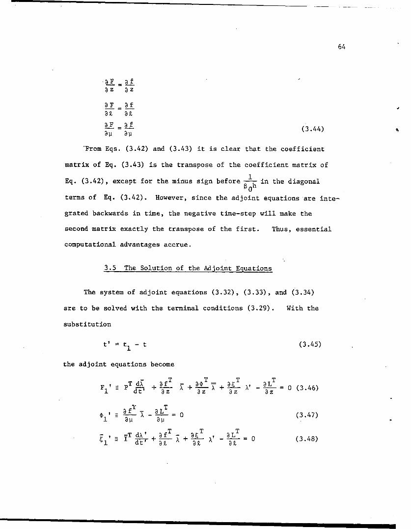
64

az az

3 F a ~f

aF a af (3.44)

"From Eqs. (3.42) and (3.43) it is clear that the coefficient

matrix of Eq. (3.43) is the transpose of the coefficient matrix of

Eq. (3.42), except for the minus sign before in the diagonal0

terms of Eq. (3.42). However, since the adjoint equations are inte-

grated backwards in time, the negative time-step will make the

second matrix exactly the transpose of the first. Thus, essential

computational advantages accrue.

3.5 The Solution of the Adjoint Equations

The system of adjoint equations (3.32), (3.33), and (3.34)

are to be solved with the terminal conditions (3.29). With the

substitution

t' = t1 - t (3.45)

the adjoint equations become

F1 pT d +-a-T + "T=X + @ V - t-T~zT 0 (3.46)

j1' 3fT azLT 3

T f @L 0 (3.47)

IT d T' + + T 3' 0

-Td-' +•f + 9? -3-z- X0 (3.48)

dtI I + i i il-I I l l l l I I

65

with the initial conditions:

T(0) = ' gt P(b)-iaZ(tl1) (3.49)

XI'(0) = •gj=0,11, .. (s-l)

2+4j a (tl)

Then the corrector coefficient matrix becomes exactly the trans-

pose of the original coefficient matrix. To make full use of the

results obtained in the process of solution of the original set

of equations of motion, the time instants (indexed), Gear constant

80 step-size, the solution variables, and the coefficient matrix

elements are stored in a direct access disk at each time grid.

The matrix elements or the G-vector of ADAMS 2-D [14] are origin-

ally arranged with column-wise representation.

To make use of the same subroutine as in the SPARSE-MATRIX

package for LU factorization of the transposed coefficient matrix,

some modifications have been made in the subroutine S08000 of ADAMS

2-D [14] to represent the transposed matrix in a column-wise manner.

It is then stored in the direct access device. It is to be noted,

however, that the time grid of the backward integration for the sol-

ution of the adjoint equations will not, in general, coincide with

the original grid. So interpolation of the original solution var-

iables and the second components of the Nordsieck vector [6,2] is re-

quired for calculation of the right-hand side of the corrector equa-

tions of the adjoint set and the integrands of the sensitivity

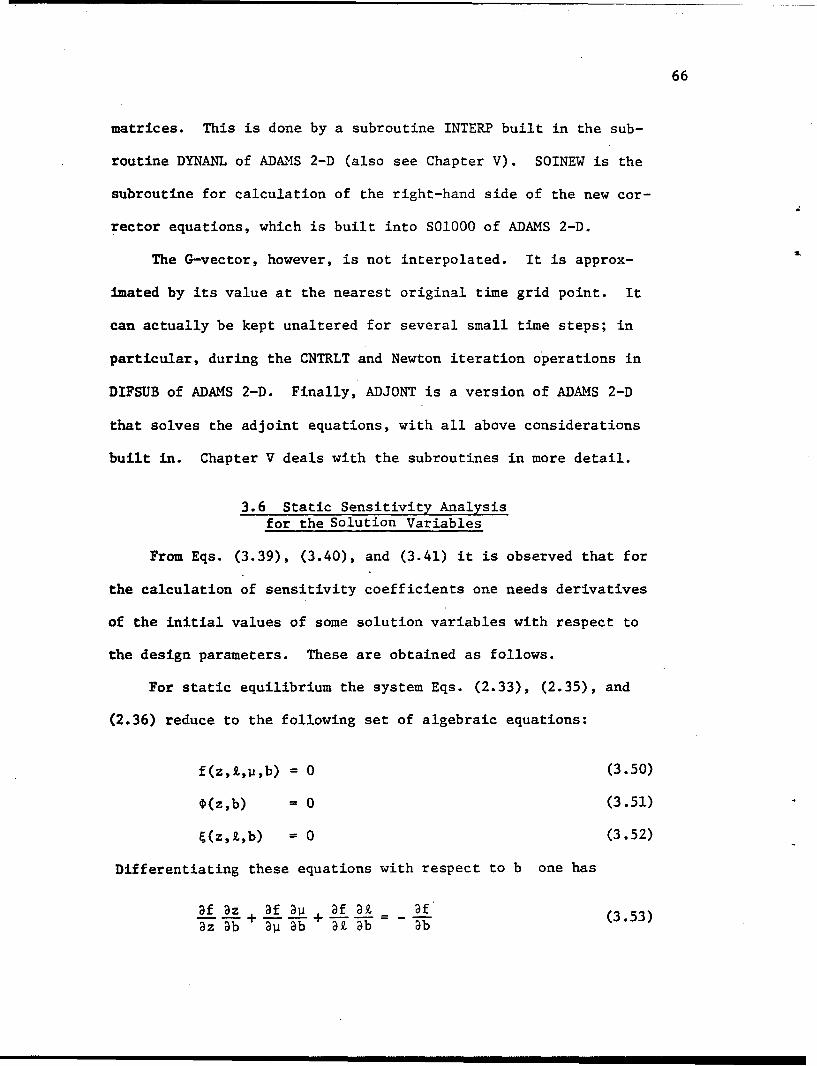
66

matrices. This is done by a subroutine INTERP built in the sub-

routine DYNANL of ADAMS 2-D (also see Chapter V). SOINEW is the

subroutine for calculation of the right-hand side of the new cor-

rector equations, which is built into S01000 of ADAMS 2-D.

The G-vector, however, is not interpolated. It is approx-

imated by its value at the nearest original time grid point. It

can actually be kept unaltered for several small time steps; in

particular, during the CNTRLT and Newton iteration operations in

DIFSUB of ADAMS 2-D. Finally, ADJONT is a version of ADAMS 2-D

that solves the adjoint equations, with all above considerations

built in. Chapter V deals with the subroutines in more detail.

3.6 Static Sensitivity Analysisfor the Solution Variables

From Eqs. (3.39), (3.40), and (3.41) it is observed that for

the calculation of sensitivity coefficients one needs derivatives

of the initial values of some solution variables with respect to

the design parameters. These are obtained as follows.

For static equilibrium the system Eqs. (2.33), (2.35), and

(2.36) reduce to the following set of algebraic equations:

f(z,1,1±,b) = 0 (3.50)

,(z,b) = 0 (3.51)

E(z,l,b) = 0 (3.52)

Differentiating these equations with respect to b one has

af 9z +f a4 + g .af . (3.53)3z Db D U @b at ý_b _ýb

67

az b- a- (3.54)

a _ a (3.55)az 3b at 3b 3b

Eqs. (3.53), (3.54), and (3.55) represent a set of (3n+2m+4s)

linear equations for Lz ap and In matrix form these eq-3b' 3b' -f

uations are equivalent to

J V • F (3.56)

where (using Eq. (3.42)),

'af af afa z YV~

J, a 4)- 0 0(3.57)

0_3z at-

is the Jacobian matrix of the static analysis and

abv- ' z b a•b (3.58)

3b'-FF 3_ _8aff , ý D a.•_ab' 8 (3.59)

The sparse matrix codes generated during static analysis are

utilized to solve for av- , with the help of the subroutine DIFSUB.

The static sensitivity analysis results for a spring-reset plow-

share mechanism (see Chapter VI) are given in Tables 6.7 and 6.8

in Chapter VI.

68

CHAPTER IV

OPTIMAL DESIGN ALGORITHM

4.1 Steepest Descent Method with ConstraintError Compensation

The general optimal design problem formulated in Chapter III

can be solved by the generalized steepest descent programming

technique presented in Ref. [E]. Here the technique will only

be discussed very briefly.

After the sensitivity analysis of Chapter III, the problem

is reduced to finding a vector 6b that minimizes 60 and corrects

constraint violations. For this purpose, the following defini-

tions are made. Define a set of indices

A = {SI*s + e > 0} (4.1)

and a column vector of c-active elements of ýS,

o= [S*.A] (4.2)

In order to assure the satisfaction of the constraints, the viol-

ations will be corrected by demanding that

6* < A 5S (4.3)

where Se A and A*S is a desired change in the constraint function

*S. Generally, AýS is chosen to be -4S"

In the notations of Chapter III, the problem reduces to

69

finding 6b to minimize

S•0pT

0 k06b (4.4)

subject to the constraints

S•-T

S=Z 6b <Ai (4.5)

and the quadratic step size constraint

T 2

6bT W 6b <n2 (4.6)

where n is a small number and W is a positive definite weighting

matrix.

The Kuhn-Tucker necessary conditions of nonlinear programming

may now be applied to solve this reduced problem. According to

the Kuhn-Tucker Theorem, it is necessary that there exist a scalar

multiplier yo > 0 and a vector of multipliers, y =Ys' Se Al

yS > 0 for inequality constraints, such that

YT(2YpT 6b - A*) = 0 (4.7)

and

3G 0 (4.8)3(6b)

whereG = t 0T 6b + yT( 0T 6b-Ap) + y 0 (6bTW~b-n 2) (4.9)

Equations (4.8) and (4.9) give

0 + Jy + 2y 0W6b =0 (4.10)

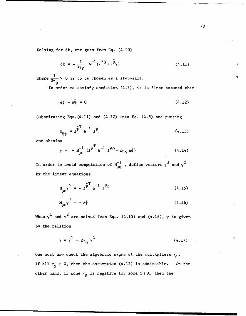
70

Solving for Sb, one gets from Eq. (4.10)

Sb = - w-l( 0O+ y) (4.11)2Y0

where 1- > 0 is to be chosen as a step-size.

In order to satisfy condition (4.7), it is first assumed that

6* - A•= 0 (4.12)

Substituting Eqs.(4.11) and (4.12) into Eq. (4.5) and putting

-TM k - W-1 (4.13)

one obtains

y =- T W-1 0 + 2 0 A+2 ) (4.14)

In order to avoid computation of M define vectors 2 and y

by the linear equations

1 = - 21T W- 1 £Z0 (4.15)

M y = - (4.16)

1 2

When y and y are solved from Eqs. (4.15) and (4.16), y is given

by the relation

yy 2y y (4.17)

One must now check the algebraic signs of the multipliers YS.

If all y.> 0, then the assumption (4.12) is admissible. On the

other hand, if some yS is negative for some SF aA, then the

71

corresponding constraint 6S- APS < 0 should have been strictly

satisfied. Therefore, 4S should be removed from P. Then a new

reduced set ý is formed and the multipliers of this new set are re-

calculated.

From Eqs. (4.17) and (4.11) one obtains

6b 1- 1 w-l*(Ž0+z 1 i - P.-i 2 (4.18)2 YoDefining

Sb1 = W'-(k0+z£' yl) (4.19)

6b2 W-1 k y2 (4.20)

the change 6b of Eq. (4.18) can be written as

1 1 26b 1 6bI + 6b (4.21)2Yo

In practice, instead of choosing n in Eq. (4.6), y0 is chosen

directly to give the step-size 2y0

The following relations can be easily shown to follow as a

necessary consequence from the above equations:

6b1T W6B2 = 0 (4.22)

.T 6b2 = Ap (4.23)

kýT Sb1 = 0 (4.24)

-Y, 0T blb < 0 (4.25)

From these relations it can be observed that:

72

(1) 6b and 6b2 are orthogonal,

2(2) 6b provides the desired constraint correction,

(3) 6b has no effect on the constraint functions in p,

and (4) Sb provides a reduction in * 0 '

A convergence criterion for this method is defined and proved

in Ref. (1]. This requires that as the optimal solution is

approached, bI converges to 0.

The choice of step-size 1is of extreme importance. It has

been observed that a very small step will result in slow converg-

ence, while a large step may cause oscillation about the minimum

point, or even divergence. Generally, the step-size is determined

by assuming that the initial estimate is in the fqasible region,

so that i = 0 and a fixed percentage reduction in the cost function

*0 is sought. If the desired change in *0 is chosen to be A*0 < 0,

then from Eqs. (4.4), (4.18), and (4.19) one obtains

1 - (4.26)

This choice is however, made at the beginning of the iterative pro-

cess and subsequently the step-size is adjusted by multiplying the

previous step-size by a factor to speed convergence or to avoid os-

cillation.

4.2 Optimal Design Algorithm

Application of the sensitivity analysis of Chapter III and the

generalized steepest descent programming technique of the previous

73

section gives the following optimal design algorithm:

Step 1: Estimate the optimum design parameter vector b

and solve the state equations of motion (2.33), (2.35), and

(2.36) for z(j) W(t ) (t) , and (t) corresponding to b wit'h

SPARSE MATRIX and STIFF INTEGRATION (GEAR) algorithms imple-

mented through the ADAMS Program and at each time step store

the solution variables, indexed time-instants, time step-size,

and corrector coefficient matrix in a direct access disk.

Step 2: Check constraints of Eqs. (3.7), (3.8), and (3.10)

and form the vector of constraint functions i, consisting of

such that 'p - e, where c > 0 is small. Also choose the

the constraint error correction vector A* - '.

Step 3: Implement a modified ADAMS program to solve the ad-

joint differential equations (3.46), (3.47), and (3.48) with

initial conditions (3.49), to obtain XQ0(t) and X ý(t), •p

corresponding to e-active constraint functions.

Step 4: Compute

*0 a go r , +[ ag 0 T o (O)P (b) ] a• + s [ g o

3 b--- + Lý 0)b b + 0

+ tp 0 ) -1y 1 _L_ - *0 T 3(P(b)i) - iT ;f

f0[T ab (b A0 VT

--• -Idt (4.27)

9b3b

74

gag F [ ag + ()P(b) + s-= b La z(O) jb X (0)j =0 La7ZFl+4j

+ 1 T (0)] a [ + rLbT a(P(b):)

•2+4j(0) a b ' -l bb

S9b a-0 j dt (4.28)

and91 W P, ,if 4iis not empty

'pip if 1~is empty (4.29)

where 9.* is the (Px ) matrix constituted of the vectors k2.,

p is the number of design parameters and 8 is the number of

violated constraints, and W is a weighting matrix [i].

Step 5: Choose step-size1 > 0 and calculate the Lagrange2y 0

multiplier vector y from

T -1 ýO* = _k£T W Z. (4.30)

and1 2

Y2OY (4.32)

Step 6: Check the algebraic sign of each component of y

associated with inequality constraints. If any components

of y are negative, redefine ' by removing the corresponding

terms from ' and return to Step 4.

75

Step 7: Compute 6bl, 6b2,and 6b from

6b1 = W- (zO 0+ kyl) (4.33)

Sb2 = W-I k Y 2 (4.34)

and

6b 1 - bl + 6b2 (4.35)2YO

6b gives a design improvement.

Step Compute b 0+l) = b(j) + 6b (4.36)

Step 9: If the constraints are satisfied and 116bl1 1 is

sufficiently small, terminate the process. Otherwise, re-

turn to Step 1 with b 0+l) as the best estimate of the design.

76

CHAPTER V

THE DYNAMIC ANALYSIS AND DESIGN SYSTEM (DADS) PROGRAM

5.1 Introduction

The Dynamic Analysis and Design System (DADS) computer program

is developed to carry out the dynamic analysis, design sensitivity

analysis, and optimal design formulations described in Chapters I-I,

III, and IV for general nonlinear mechanical systems. Provisions

for regenerating sparse-matrix codes at necessary time instants of

dynamic and adjoint analyses have been made so that the program can

handle systems with intermittent motions (see Plow-share mechanism

in Chapter VI (Section 6.3)) with sufficient ease.

The DADS program executes in two main phases: (1) The dynamic

analysis phase and (2) The sensitivity analysis and optimization

phase. The dynamic analysis phase of the program generates the

sparse matrix code for pivoting and LU factorization of the Jacobian

matrix and solves the differential-algebraic equations for the state

variables during a specified time interval. It employs sparse

matrix codes and the numerical integration routine presented in

Chapters II and III. It then stores the Jacobian matrix and state

variables on a direct access disk for use in the sensitivity analysis

phase. The dynamic analysis phase also performs static sensitivity

analysis for the solution variables (see Section 3.6).

The sensitivity analysis and optimization phase of the program

77

incorporates the techniques of Chapter IV into various subprograms

and solves adjoint equations (see Section 3.3) using the data stored

on disk. The same numerical integration subroutine is used to

solve the adjoint equations. The program further computes sensiti-

vity coefficients and the necessary design improvements. The pro-

cess is repeated until optimum results are achieved.

5.2 Main Features of DADS Computer Program

The DADS program has the following features:

(1) The mechanical systems treated are discrete, nonlinear, and

constrainted (two-dimensional at present);

(2) General nodal formulation of equations of motion for the

bodies [7];

(3) Necessary data being given, formulation of the equations of

motion and the Jacobian matrix is automatic;

(4) Integration of a combined set of differential and algebraic

equations (DAE) is performed;

(5) The following three algorithms are used:

(a) Newton iteration;

(b) Sparse Matrix techniques for the solution of the linearized

simultaneous equations;

(c) Stiff Integration Algorithm (GEAR) for numerical integration.

(6) Types of analyses performed:

(a) Static analysis;

(b) Transient analysis;

78

Wc Static sensitivity analysis f or solution variables;

(d) General design sensitivity analysis;

(e) Optimal design.

The static and transient analysis part of the program was

mainly developed by Orlandea [7] and Wehage [14]. The correspond-

ing references are recommended for further details. Fig. 5.1 shows

An outline of DADS program capabilities, Fig. 5.2 shows the main

subroutines used in the dynamic analysis phase of DADS, and Fig. 5.3

identifies the main subprograms used in the design sensitivity anal-

ysis and optimization phase, and Fig. 5.4 is a flow diagram of the

DADS computer program.

5.3 Brief Description of the Dynamic Analysis Phase

.The dynamic analysis phase (DYNANL) of the DADS program in-

volves establishing the sparse matrix code description of the mechan-

ical system and solving the differential and algebraic equations for

the state variables. As shown in Fig. 5.2, this involves two major

steps: Ci) generation of an initial sparse matrix code (including

pivoting and LU factorization code) and (ii) repetitive solution of

linearized equations for the state variables during the time interval

of interest.

In the first step of dynamic analysis, estimates of the initial

configuration of the system are provided by INDATA and are used by

VARSET to initialize a state variable vector for subsequent use by

the numerical integration routine DIFSUB. A compact numbering

79

-40

to 0.,o :$ $ -

.d -Hc

Um WCA 4cn) 0) n

44 ?-1 ý4 t

44 ca o 4L

0 w 0 r 0 w 4

w -cc r w

80

cn

CA w

00

CRC

o Co -WE-

rrA

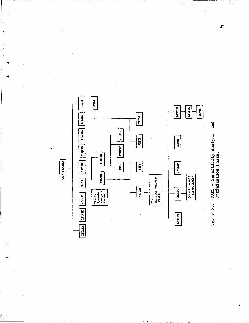
81

.,A

ni

-H A__ 0L0Cc I

P.<p

7.4

82

SRead initial estimates, bounds, number of constraints, 1and other parameters related to the design problem

J4

Initialize system parameters for implementation ofthe ADAMS-2D program

(INDATA)

Relate design parameters with system parameters I(RELATE)

Find the solution of the equations of motion byADAMS-2D program and store the results in disk

(ADAMS 2)

Evaluate integrands of cost and constraint functions(HALS)

Solve adjoint equations and find the sensitivity mat-rices for the violated functional constraints

(INFUNC, TEQFUN, ADJONT, AHLPSI)

Test the design parameter constraints and find thesensitivity matrices

(DPARMC)

Find the sensitivity vector £X 0 P

(AHLPSI)

Compute MN, and the Lagrange Multipliers, check theirsigns, and compute design improvements

(NEWB)

Test the convergence criteria

Figure 5.4. Flow Diagram of the DADS ComputerProgram.

83

system identifying bodies, joints, and spring-damper elements is

4 used to input data through VARSET and provides the necessary des-

cription of the mechanical system configuration. These data are

used to construct the Newton corrector state equation (3.42) and the

system of adjoint equations (3.43) (for use in the sensitivity anal-

ysis phase). This information is used in S03000 to generate init-

ial vectors of row and column indices for nonzero entries in the

Jacobian matrix and to assemble the standard equations that are re-

quired on the right hand side of Eq. (3.42). Similarly, descrip-

tions of user-supplied row-column positions of additional non-

standard elements are provided by incorporating the necessary code

in USET. A symbolic description of the resultant matrix is

printed by DEBUGG for reference purposes and a column-ordering perm-

utation vector is generated in S08000.

Subroutine SOl000 evaluates the Jacobian matrix and right hand

side of Eq. (3.42). Its purpose is to (i) evaluate force and dis-

placement functions of time that are provided by the user through

subroutine FOREXT, (ii) transfer the state variables from a single

vector used by the numerical integration routine to the standard var-

iables (and user-supplied variables through USOLVl), (iii) evaluate

that part of the Jacobian matrix that is associated with the standard

equations (and user-supplied equations, USO0V2), using updated var-

iables from step (ii) and the previously generated column-ordering

permutation vector (S08000), and (iv) evaluate the standard equations

84

(and user-supplied equations, USOLV3). Subroutines LSPTRS, LSSLV1,

LSSLV2, and LSSLV3 are included as user-supplied routines to incor-

porate nonstandard highly nonlinear springs and dampers, as described

in the plow share mechanism example of Chapter VI. Finally a sparse

LU factored description of the matrix is generated in subroutine

INVERT.

The second step of dynamic analysis is then to numerically inte-

grate the system of equations during the time interval of interest.

This is accomplished by the numerical integration subroutine DIFSUB,

which repeatedly calls SOl000 to update the Jacobian matrix and system

of equations as it executes the iterative corrector formula of Eq.

(3.42). The Jacobian matrix and the results of numerical integration

are stored in a direct access disk.

In sensitivity analysis, DYNANL is called in ADJONT (adjoint anal-

ysis phase) (Fig. 5.4), which is again called in AHLPSI, where the

sensitivity coefficients are calculated. For this case, DYNANL reads

stored data from the disk and passes through two distinct steps. In

the first step, the sparse matrix codes for pivoting and LU factoriz-

ation are generated for the transpose of the Jacobian matrix, through

INVERT. In the second step, the system of adjoint equations (3.32)

to (3.34) are numerically integrated through DIFSUB, which repeatedly

reads data from the disk, calls SONEW for the evaluation of the

right-hand sides of the adjoint system, solves the adjoint variables

at various time steps, and stores the solution results on a disk for

use in the calculation of sensitivity coefficients.

85

5.4 Description of-the DADS Program

As noted in Section 5.1, the computer program DADS is consti-

tuted of two main phases: (i) Dynamic Analysis phase, and, (ii)

design sensitivity analysis and optimization phase. The main flow

of the program is described below (see also Fig. 5.4).

In the main program, the initial estimates and bounds on de-

sign parameters, number of constraints, stepsize, percentage of

cost function reduction, and other parameters related to the design

problem (see Chapters III and IV) are read. Then system parameters,

such as masses, moments of inertia, locations of centers of masses,

applied constant forces, joint types, and spring-damper parameters

are read, through the subroutine INDATA. The subroutine RELATE

relates the variables and parameters of the dynamic analysis (ADAMS 2

and DYNANL; see also Section 2.1 of Chapter II) to the updated de-

signparameters (Chapters III and IV).

For dynamic analysis, DYNANL is called through ADAMS2. The

Jacobian matrix, solution variables, time step, time instant, and

order of numerical integration are then stored in a direct adcess

disk. They are first used to evaluate the integrands of the cost

and constraint functionals of Eqs. (3.1), (3.6), (3.7), and (3.11),

through subroutine HALS.

Next, the inequality functional constraints.of Eqs. (3.7) and

(3.10) are tested and the corresponding adjoint equations (3.32) to

(3.34) are solved through INFUNC, TEQFUN, AHLPSI, and ADJONT. At

this stage, DYNANL (Adjoint Analysis Phase) is called by subroutine

86

ADJONT, The matrix of sensitivity coefficients k (see Eq. (3.41))

is calculated for the violated functional constraints through AHLPSI.

The subroutine DPARMC then tests the design parameter constraints

and calculates the corresponding design sensitivity vectors. The sensi-

tivity vector Z 0 of Eq. (3.40) is then calculated through AHLPSI. The

subroutine NEWB then computes the matrix M of Eq. (4.29), solves Eqs.

1 2(4.30) and (4.31) for y and y , and computes the design change Sb

given by Eqs. (4.33) through (4.35).

At this stage, convergence criteria are tested. If they are sat-

isfied, the new design is taken as the optimum one. Otherwise, the

process is repeated with the new design paramters used as the initial de-

sign estimate.

In the following sections, descriptions of the principal program

variables and subroutines are presented.

5.4.1 Principal Variables

a) Dynamic Analysis

TIMPU - current time

NB - number of bodies including fixed body 1

NJ - number of joints

NSD - number of spring-damper pairs

NSDV - twice the number of nonlinear spring-damper pairs

NSDT - number of torsional spring-damper pairs

EPS - maximum one-step error in numerical integration

M - vector of masses of the bodies

87

JIN - vector of moments of inertia

X, Y - coordinates of the CM's with respect to inertialreference frame

PHI - angular displacements of X-axis of bodies withrespect to inertial refernece frame X-axis

FX, FY - components of the force applied at CM parallel tothe inertial reference frame axes

TQ - applied torques

JT - type of the joints

IB(I,I),IB(2,I) - numbers given to the two neighboring bodiesconnected by the ith joint

Xl, Yl - co-ordinates of the revolute joint or a point onthe axis of the translational joint with respectto the axes of the first body

X2, Y2 - same as above with respect to the 2 nd body

IBSD(I,I),IBSD(2,I) - numbers given to the two bodies connectedby the ith spring-damper pair

XFl,YFI - co-ordinates of the point of attachment on the firstbody with respect to the body fixed axes

XF2,YF2 - same as above with respect to the 2nd body

SK - spring constants

DC - damping coefficients

SDL - deformed spring lengths

SDLO - undeformed spring lengths

SDF - constant forces applied along spring-damper pairs

IBSDT(I,I),IBSDT(2,I) - numbers given to the two bodies con-nected by the ith torsional spring-damper pairs

SKT - torsional spring constants

DCT - torsional damping coefficients

88

PHIO -initial difference of the angular displacementsof the bodies for the undeformed torsionalspring-dampers

TQO - constant couples applied at the torsional spring-

damper pairs

V - the time-derivatives of SDL's

FFX,FFY - components of the spring-damper forces with res-pect to inertial reference frame

TQS - torsional spring-damper couples

UX,UY - components of the velocities of the CM's with res-pect to inertial reference frame

UP - angular velocities of the bodies with respect to

inertial reference frame

LM - Lagrange multipliers of the dynamic analysis

G - vector of column-ordered nonzero elements in theJacobian matrix

CL - right-hand sides of the corrector equations

JSIZ - size of the Jacobian matrix

NPOS - pointer to consecutive nonzero positions in theJacobian matrix.

b) Sensitivity Analysis and Optimization Phase

The principal variables occurring in the program, over and above

those mentioned above are described below.

NBl - number of design parameters (total)

NAB - number of artificial design parameters

MS - expected size of constraint set

NFCE - number of pure equality functional constraints

NFCET - number of transformed equality functional con-straints

89

NFCI - number of inequality functional constraints

NDCI - number of design parameter constaints

NPl - number of time grids in stiff integration inADAMS 2

B - design parameters

BI - starting values of the design parameters

BL - lower bounds of the design parameters

BU - upper bounds of the design parameters

COSTJ - cost function

EPE - tolerance for equality functional constraints

EPI - tolerance for inequality functional constraints

EPDI - tolerance for design parameter constraints

ER - convergence criterion

ILIM - limit of iterations in optimization program step

W - weighted matrix (generally diagonal)

NP2 - number of time grids in stiff integration inADJONT

ALM - adjoint variable

Gl - vector of column-ordered nonzero elements in thetransposed Jacobian matrix

MPOS - a vector playing the same role in adjoint anal-ysis as NPOS in dynamic analysis (see Chapter II)

NPOSRR - a copy of original NPOSR (S(see Chapter II)

JPMA - a copy of JP9

ALS - the integrands of the cost and constraint func-tionals

GS - non-integral parts of the cost and constraintfunctional

90

AHSMT - maxima of the integrands of the transformedequality constraints

DLDZ - derivatives of the integrands of the cost andconstraints functionals with respect to thestate variables (both primary and secondary)

HLJ - sensitivity coefficients for the cost functional

HLPSI - sensitivity coefficients for the constraintsfunctionals

PSIC - constraint functionals

NCV - number of constraint violations

NCVID - indices of the violated constraints

Some other variables are defined during the description of the

subprograms in the next section.

5.4.2 Description of the Subprograms

In this subsection a brief description of each of the main sub-

programs of DADS is given and some of the call-list variables not

appearing in the previous subsection are explained briefly.

SUBROUTINE INDATA (IECHO, ALM)

The subroutine INDATA reads input data that characterizes the

mechanical system. It also reads initial values of adjoint variables

and the maximum values of nonlinear spring-damper pairs into the pro-

gram.

IECHO - a logic variable for writing the data on paper

- 0, data is not written,

- 1, data is written.

SUBROUTINE RELATE (YY, IMODE)

The subroutine RELATE relates the parameters and variables of the

91

dynamic analysis to the updated design parameters.

YY - an array which contains the dependent variables (dynamic

analysis) and their derivatives. Its dimension should be at least

(JSIZ,7) where JSIZ is the Jacobian size.

IMODE - a logic variable characterizing the type of analysis per-

formed,

- 0, neither static nor dynamic analysis,

1 1, static analysis,

- 2, dynamic analysis.

SUBROUTINE ADAMS2(IFLAG1, SOLNO, JSIZ, DLDB, DFDB, DPHDB,

DZIDB, YY, PB, ALM, DNDB)

The subroutine ADAMS2 feeds in some flags, time step, maximum

and minimum time steps, and calls subroutine DYNANL to initiate tran-

ient solution.

IFLAGl - a logic variable,

= 0, for dynamic analysis,

= 1, for adjoint analysis.

SOLNO - an integer keeping a running acount of the solution num-

bers at different time steps during dynamic analysis.

DLDB - derivatives of the integrands of the cost and constraint

functionals with respect to b (design parameters).

DFDBderivatives of the equations of motion, constraint

DPHDB-equations and spring-damper relations with respect to b.

DZIDB

PB -elements of P matrix in equations of motion.

92

DNDB - derivatives of the initial solution variables with res-

pect to b,

SUBROUTINE HALS(NPI,YY,JSIZ)

The subroutine HALS evaluates the integrands of the cost and con-

straint functionals at each time step.

SUBROUTINE INFUNC(TMAX,ITR,EPI,NFCI,NCV,JSIZ,YY,DLDB,

DPHDB,DZIDB,DPDFZT,DNDB,DGDB,DGDZ,DPDB,PB,ALM)

The subroutine INFUNC calculates, through the subroutine AHLPSI,

the sensitivity coefficients for the inequality functional constraints

(Eqs. (3.10)).

ITR - running number of optimiaztion iterations

DGDB - derivatives of the non-integral parts of the cost andconstraint functionals with respect to b

DGDZ - same with respect to initial state variables

DPDB - derivatives of P matrix with respect to b.

SUBROUTINE TEQFUN(TMAX,ITR,EPE,NFCE,NFCET,NCV,JSIZ,YY,DLDB,

DFDB,DPHDB,DZIDB,DPDFZT,DNDB,DGDB,DGDZ,DPDB,PB,ALM)

The subroutine TEQFUN calculates design sensitivity coefficients

for the transformed equality functional constraints (Eqs. (3.7)).

SUBROUTINE DPARMC(TMAX,ITR,EPDI,NDCI,NCV)

The subroutine DPARMC calcualtes design sensitivity coefficients

for the design parameter constraints (Eqs. (3.8)).

SUBROUTINE AHLPSI(NCV,ITR,TMAX,ISO,DLDB,DFDB,DPHDB,DZIDB,

DPDFZT, DNDB,DGDB,DGDZ,DPDB,PB,YY,JSIZ,ALM)

The subroutine AHLPSI calculates design sensitivity coefficients

93

for the constraints and cost functionals, with the help of sub-

routines ADJONT, PBFN, ADPDB, and DGDBZ.

ISO - running number of the functional constraint treated.

SUBROUTINE NEWB (EPS ,NCV, STEP, ITR, NFCV)

The subroutine NEWB computes the matrix M of Eq. (4.29),

1 2solved Eqs. (4.30) and (4.31) for y and y , and computes the nec-

essary design changes 6b given by Eqs. (4.33) through (4.35).

STEP - desired reuction in cost functional

NFCV - number of total functional constraint violations.

SUBROUTINE DYNANL(IS , IECHO, ITROB,TMIN, TMAX,TSTEP,HMIN,

HAMX,H,DLDB,DFDB,DPHDB,DZIDB,JSIZ,YY,PB,AIM,LIN,TLIMIT,.

EPS, IFLAGI, SOLNO, SOLNOI,ISO, DNDB)

Subroutine DYNANL is described in detail in Section 5.3.

IS - a logic variable,

0, for static code generation,

1, for static solution,

2, for dynamic code generation,

3, for dynamic solution.

LIN - a user-supplied flag that limits the number of cor-rector iterations to 1 if all equations are linear,

0, for linear equations

1, for nonlinear equations.

SOLNO - an integer keeping a running account of the solutionnumbers at different time steps during adjoint analysis.

SUBROUTINE ADJONT(ISO, IFLAGI, SOLNOl,DLDB,DFDB,DPHDB,DZIDB,

JSIZ ,YY,PB,ALM,DNDB)

94

The subroutine ADJONT works in a similar manner as ADAMS2 to

solve the adjoint equations.

FAMCTION AHSM(I)

The function subprogram AHSM determines the maxima of the integrands

of the transformed equality constraints, which are used in TEQFUN.

FUNCTION FUNPSE(I,TMAX)

The function subprogram FUNPSE evaluates the values of the func-

tional constraints and the cost functional.

. SUBROUTINE PBFN(PB)

The subroutine PBFN calculates terms of the P(b) matrix.

SUBROUTINE ADPDB (DPDB,PB)

The subroutine ADPDB calculates derivatives of the P(b) matrix

with respect to design parameters.

SUBROUTINE DGDBZ(DGDB,DGDZ,ISO)

The subroutine DGDBZ calculates the derivatives of the non-inte-

gral parts of the cost and constraint functionals.

SUBROUTINE DLDFB(TIMPU,ISO,YY,JSIZ,DLDB,DFDB,DPHDB,DZIDB)

The subroutine DLDFB calcualtes the derivatives 3L 9f aS' 3b

and afor sensitivity analysis.ab

SUBROUTINE SO1NEW(ISO,JSIZ,HB,PB,AB,AIM,A,T,TIME,ZMAX)

The subroutine SOINEW calculates the right-hand sides of the

corrector euqations for the adjoint system.

HB - time step of dynamic analysis

AB - transformed gear coefficients of dynamic analysis usedin adjoint analysis

A - current transformed gear coefficients

95

T - current time step

TIME - current time

ZMAX - total time interval of dynamic analysis.

SUBROUTINE ADLDZ(ISO,JSIZ,TIME,ZMAX)

The subroutine ADLDZ calculates the derivatives hz of the

integrands of the cost and constraint functionals with repsect to sol-

ution variables of the transient analysis.

SUBROUTINE INTERP(Y,N,TA1,NP3,TMAX,JSTAT1)

The subroutine INTERP computes interpolated values of the depen-

dent Variable Y(I,1) and its time derivatives and replaces the previous

values. The interpolation is to the point TOUT and uses the Nordsieck

history array Y as follows:

JSTATIY(II) = I Y (I, J+1)*S**J,

J=Oand

JSTATlY(I,2) = I J*Y(I,J+l)*S**(J-I),

J=lwhere

S = (TOUT+TA(NP3) - TMAX)/HA,

TA(NP3) is an old time instant during backward integration and HA is

the time step of dynamic analysis.

SUBROUTINE VARSET(YY)

The subroutine VARSET sets the variable YY to be used in DIFSUB

for numerical integration

SUBROUTINE S03000(NB,NJ,IB,JT,NSD,IBSD,NPSOR,NPOSC,NG,NT,

JSIZ,ITF,NPSS,NSDT,IBSDT,IMODE)

96

The subroutine S03000 sets up pointers of the sparse matrix non-

zero position.NPOSR - pointer for the row number of each nonzero entry

NPOSC - pointer to the column number of each nonzero entry

NG - an integer variable keeping a running index of allthe row and column pointers to the nonzero entriesin the Jacobian matrix

NT - a vector giving values of NG after execution of diff-erent segments of S03000

ITF - a flag for keeping 10 nonzero positions for a revolutejoint and 14 for a translational joint

NPSS - a vector storing different NG's at the beginning of each

block of nonzero positions for a body in the Jacobian.

SUBROUTINE SOIO00(T,A,H,JSIZ,IMODE,YY,IFLAG1,PB,AB,ISO)

The subroutine S01000 mainly updates the terms of the Jacobian

matrix and the right hand-side terms of the corrector equation (see

Section 5.3 for further details).

SUBROUTINE INVERT(G,JSIZ,NP2,IP,JU,JC,IXL,IXH,IPP,ICNT,IPR,

IPC,IPRI,IVA,IVL,IVU,IC,IU ,JA,IRP,IRL,IWSR,ICP,ICL,IWSC,

IRWM,IRWC,AT,MAXS,MAXN,IB,NPOS,IMODE,ITF,NPSS,IFLAG1,IPSAV,

JASAV,IKNT,KFLAG)

The subroutine INVERT orders a matrix optimally and generates and

stores sparse matrix codes for LU factorization. Provisions have been

made in the program to call it in DYNANL whenever necessary during tran-

sient and adjoint analyses.

SUBROUTINE DIFSUB(N,TIME,T, TMIN,TMAX,EPS,YMAX,ERROR,KFLAG,

JSTART, MAXDER,G,IVPTR,NERR,NRR,NAL,LIN,CS,DY,TDIV,NCONV,

97

NPOS,JA,IP,IVA,IC,IU,JC,JU,DI,CC,U,IVL,IVU,CL,IPR,IPC,

Ak IPRI,TLIMIT,IW1,TNEW,NQ,Y,YS,IFLAG1,PB,AB,ISO,A,HA,

ZMAX, TA,NP3, JSTAT1, PTEST, IKNT)

The subroutine DIFSUB is the numerical integration routine based on

the gear algorithm(Chapter II) and is of extreme importance. For an

original listing and explanation of the program and variables, refer-

ence [7] is recommended.

Explanations of the sparse matrix variables in subroutines INVERT

and DIFSUB are available in reference [61].

98

CHAPTER VI

APPLICATIONS AND NUMERICAL RESULTS

6.1 Introduction

From the structure of the computer program DADS described in the

previous chapter, it is clear that large classes of mechanical design

problems can be handled through its implementation. To test the

program, two example problems have been considered in the following

sections: (1) a slider-crank mechanism (as described in Chapter II;

see Figure 2.5), and (2) a trip plowshare mechanism.

The slider-crank mechanism is often used in engines and machiner-

ies [71] (see Chapter II) and thus it is quite familiar. The trip

plowshare mechanism treated is a simplified version of the 2500 semi-

integral spring-reset plow which is in production at John Deere

(see Section 6.3). The importance of such mechanisms needs little

description.

6.2 The Slider-Crank Mechanism

The slider-crank mechanism to be considered here is described in

Chapter II (Subsection 2.1.2.5). Figure 2.5 shows the approximate

initial position of such a mechanism with one spring-damper pair.

Link 1 is ground, link 2 is the crank shaft, link 3 is the connecting

rod or coupler, and link 4 is the piston or simply slider. A spring-

damper pair is attached between link 4 and ground (Figure 2.5). There

99

is a translational joint (type 2) between bodies 4 and 1 and one

revolute joint (type 1) between each of the following pairs of bodies:

1 and 2, 2 and 3, and 3 and 4. Gravitational forces are excluded from

the present simulation of the mechanism.

The two-dimensional ADAMS program [14] has been implemented through

the subroutine ADAMS2 to obtain a static equilibrium configuration and

to determine the subsequent transient motion. The results of this

analysis are used later in sensitivity analysis and optimization.

A symbolic listing of the nonzero positions of the Jacobian matrix

for this example problem is given in Fig. 2.7. An explanation of the

nonzero positions can be obtained in reference [14].

6.2.1 Formulation of the Optimal Design Problem

By virtue of its movement, a radial slider-crank mechanism exerts

a force on ground through the crank-bearing and the wrist-pin guide

(such as cylinder wall in an automotive piston-type engine). It is

desirable to keep these "shaking forces" within bounds. It is also

desirable to put an upper bound on the angular velocity of the crank

at the final instant T of the time-interval [0,T] under consideration.

The cost function is chosen to be twice the maximum energy stored in

the spring during the interval of motion. The following design param-

eters are considered (see Chapter II):

bI = The spring constant K1 of the spring

b2 = Height of the points of attachment of the spring

b3 = Half of the length of the uniform coupler.

100

With the notations of Chapters II and III, the optimal design

problem is stated as follows: minimize

J- max bl(YI-0 ) (6.1)0<t<T

subject to the equations of motion (2.33), the equations of con-

straints on motion (2.35), the spring-damper relations (2.36), the

initial conditions of the form of Eqs. (3.4), and (3.5), the func-

tional constraints

Iv 21 <i 2 (max) , 0 < t < T (6.2)

ý 2 (T) <$2(max) (6.3)

and the design parameter constraints

L < .bL < b. < b. , i=l,2,3 (6.4)

In Eq. (6.2) P2 is the y-component of reaction forces acting

on body 2 at joint 1, because from Eq. (2.19) y= - 1,2• 2 22and~~a so "' 8y 2 = 2 i q 22)

For the sake of simplicity, only the constraints on the vert-

ical component of shaking forces at the crank bearing have been

considered here.

After the introduction of an artificial design parameter b4

[24,35,37] and the integral functional forms in the conventional

way [24], the problem can be reformulated as: minimize

ý0 = b 4 (6.5)

101

subject to Eqs. (2.33),. (2.35), (2.36), (3.4) and (3.5), the

constraints

4 1 = jo <7 2-" 2 (max)>dt = 0 (6.6)

4T

4)2 = <P 2 -P 2 (max)>dt = 0 (6.7)

4 O3 2<b1 (J.I-2k10) - b4>dt = 0 (6.8)

4-4 42 (T) - $2(max) < 0 (6.9)

and the design parameter constraints of Eq. (6.4).

The symbol <i(t)> used above has the following meaning (see

Chapter III):

2

(t)> n(t)) for n(t) > 0 (6.10)

0 , for n(t) < 0

This formulation corresponds to the general formulation of the

optimal design problem stated in Chapter III. After specification

of initial numerical data, the DADS program described in Chapter V

can be implemented to obtain a solution.

6.2.2 Sensitivity Analysis

In problems of optimal design, sensitivity analysis constitutes

a principal part of the work to be done. When sensitivity coeffic-

ients are obtained, an iterative optimization algorithm can be

applied to determine an optimal solution. In the present class of

problems, subroutines RELATE, DNUDB, DGDBZ, ADLDZ, and DLDFB are the

major user-supplied subprograms for sensitivity analysis. Among

102

them DGDBZ and ADLDZ are often relatively simpler, because they

depend solely on the forms of the functional constraints. The rela-

tions entering into the subroutines RELATE, DGDBZ, ADLDZ, and DLDFB

for the present problem (with 1 second interval) and the plow-share

mechanism are given in the Appendix. Subroutines DGDBZ and DLDFB

are used in AHLPSI to calculate sensitivity coefficients.

6.2.3 Numerical Results

Initial estimates of the parameters for the slider-crank

mechanism under consideration are given in Table 6.1. The units

used are inch, pound-force, and second. Two time intervals are

treated: [0.0,1.0] and [0.0, 2.0]. During transient analysis a

constant counter-clockwise torque of 100 in/lbf is applied to link

2. Fig. 6.2 gives the tableau of nonzero positions of the Jacobian

matrix for thisproblem.

To examine the correctness of Eqs. (3.40) and (3.41) for

sensitivity analysis, the sensitivity coefficeints k 8 ,8c1,2,3,4}

and 0 are first calculated for the 2 second interval, with initial

estimates b' = [1.0,0.5,10.0,14.5]T for the design parameters, for

lower bounds bL = [0.8,0.2,5.0]T and upper bounds bU = [1.5,0.8,16.0]T

on the first three design parameters, and with p 2(max) = 10.0 and

$2(max) - 0.3. The cost and constraint functionals are evaluated

for 0.1% and 1.0% perturbations of the first, second, and fourth de-

sign parameters (in conjunction with 0.01% and 0.1% changes in the

third) and the corresponding changes in the functionals are exam-

ined. Table 6.2 gives the sensitivity coefficients 4 and Z

103

Table 6.1

* Initial Estimates of the Parameters for the Slider-CrankMechanism (Inch, Pound-Force, Second).

LINK DESCRIPTION

M(1) =1. M(2) =4. M(3) =1. M(4) =3.

JIN(1) = 1. JIN(2) = 10. JIN(3) =4. JIN(4) =2.

X(1) = 0. X(2) =1. X(3) =8.667 X(4) =17.32

Y(l) =0. Y(2) =0. Y(3) =5.25 Y(4) =.5

PHI(l) =0. PHI(2) =1.5708 PHI(3) =-.5236 PHI(4) =0.

FX(l) = 0. FX(2) = 0. FX(3) = 0. FX(4) = 0.

FY(l) = 0. FY(2) = 0. FY(3) =0. FY(4) = 0.

TQ(l) = 0. TQ(2) = 0. TQ(3) = 0. TQ(4) = 0.

JOINT DESCRIPTION

IB(I,l) =1 IB(I,2)= 2 IB(I,3)= 3 IB(I,4) =4

Xl(l) =0. Xl(2) =9.0 Xl(3) =10. Xl(4) =0.

Yl(l) =0. Yl(2) =0. Yl(3) =0. Y1(4) =0.5

IB(2,1) =2 IB(2,2)= 3 IB(2,3)= 4 IB(2,4) =1

X2(l) = -1. X2(2) = -10. X2(3) =0. X2(4) =0.

Y2(l) =0. Y2(2) =0. Y2(3) =0. Y2(4) =1.0

SPRING-DAMPER DESCRIPTION

IBSD(1,I)=l XFl (1) = 35. YF1 (i) = 0.5 IBSD(2, 1)= 4

XF2(1) = 2. YF2 (1) = 0. SK(l) = 1. DC(l) = 1.

SDL(1) = 15.68 SDL0(1)= 15.68 SDF(1) = 0.

104

C0

-Z

C* 0C0 D 0

*1 en

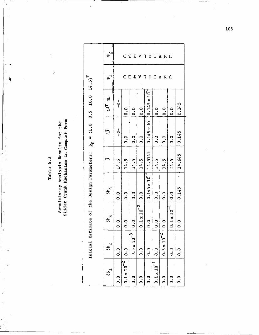
105

Q aI V 101IAINfl

0I -It

0 COD C)0 C X

o Ln u0 0 -T --T

-H 0 0 0 ,

0t IT -- -It -r

H c000 H 000 t0 0 00 0 0

cu mf u t

0) (fl 0r. H -- H H 0 H -H

Cu~ CU C 1

CD a0 -r Ll

10

C0000 H 000 HOC

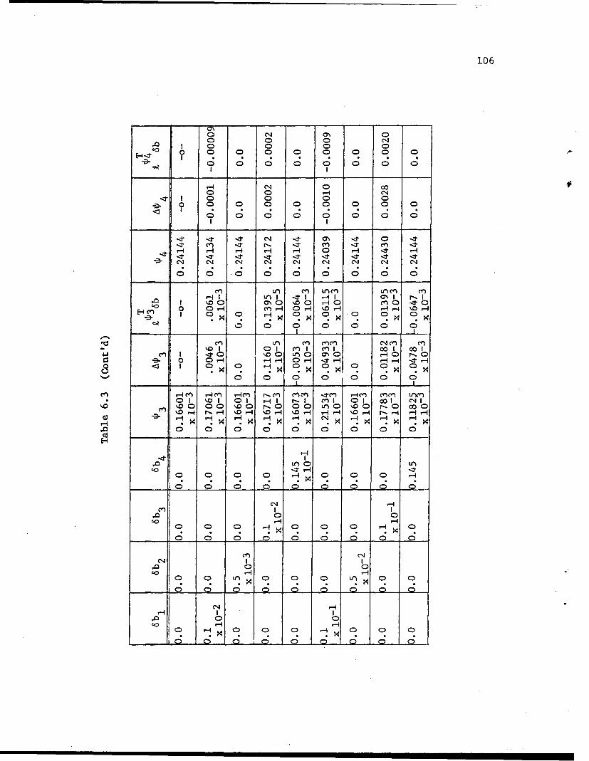
106

0 o 0 CD 0 0 0 0

0- 0 0 00o 0 0 0 0 0 C0

0 a<H

-:T -t -:T C4 It m' It 0 -

:r cn -It r- -It cn - ~ cnH- H- H- v H- H- T 0 H -ýT H-

C4I N' C'4l c' C14 C14 C14 C14 CN~

cnLf M Lncn1 Lne C Cf,HIq Ln I TON r-%I

I 10 0I H 10 rI110 0 0 ItCI~ 0 0> rIn I C)r 10 0- r- 0 0 q

IJ a l c I -cn 1 00 1r~ 0'. HO 1-W cn o 0 HD'DL 0 a%0 0 0 r 0

0; a 0 0 0 0 0

H-iC' r-4 Hc r-q M r cn Ie -~r H-en mm~ LrycnC* 0D I %D1 01 H.qI r- I cn 1 01 cat1 C~jI

%D0 m .00 00 '.00C r-..a 00 Lnb 0 100 r- 0 00oa) ~~r-H r0H %D0 '.0H %D '. - riýo HI r--H 1- H-

C0 0 0 0 0 0 0 0

CU - - - -- f--

0 0 0 ; 0 H 0 0 0D H

0m 0a 0

0) C 0 0 C

0 0L 10 0

~0f 0* CDX CD n n D CD C

CD a

SCD CD CD 'c CD 0 0 CD

107

aF {3,4}, and Table 6. 3 gives other computational results in

compact form. The first and second constraints, however, remain

unviolated.

In these computations the integrands of 41, 1 2, and i 3 have2 2 2

been normalized by dividing by 12(max)' 2(max)' and b respect-

ively. It is observed from the Table that terms of the form

*Tk Sb match satisfactorily with the corresponding Alp's. The slight

discrepancies are attributed to various approximations and lineariz-

ations at many steps of both transient and sensitivity analysis and

relatively coarse time grids for numerical integrations and trans-

formation of pointwise constraints to functional forms. However,

they need not affect the optimization process.

In carrying out the optimal design algorithm, a design reduct-

ion ratio of 3% is used to compute the stepsize in the first iter-

ation. The bounds bL and bU are taken to be [0.8,0.2,9.0]T and

[1.5,0.8,12.0] T, respectively. The initial estimate bI (including

artificial design parameter) is taken as [0.8244, 0.5, 9.0, 11.12]T

and W2 (max) and P2 (max) are kept unchanged.

At the starting design, 116b'1 1 =*0.1248 and 116b 2 11 = 0.2307,

constraints 3 and 4 are violated, and the constraint on the design

parameter b3 is tight. After 6 iterations, as the algorithm

approaches the optimum design, 1 6b'1 1 reduces to 0.8404x 10-15,

I16b211 reduces to 0.2669x10-1, and the constraints on bV, b2 , and

b3 become tight. The final optimum results are given in Table

6.4.

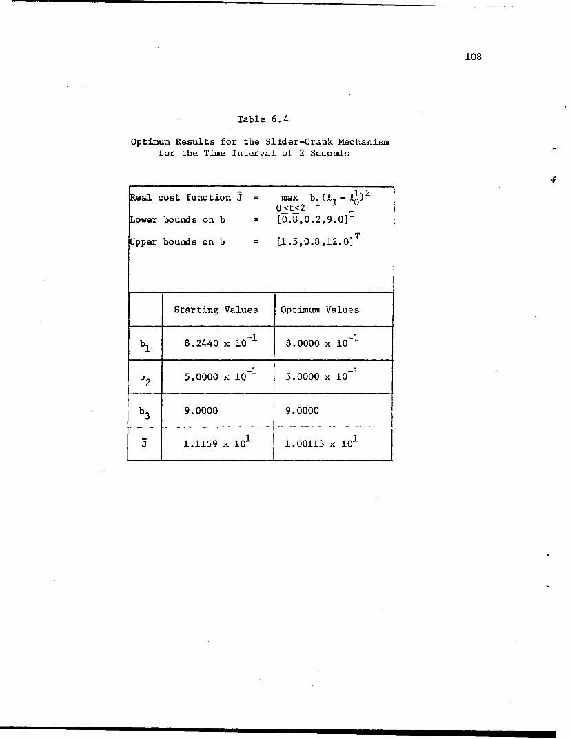
108

Table 6.4

Optimum Results for the Slider-Crank Mechanismfor the Time Interval of 2 Seconds

Real cost function J max b( 1 ( 1)20 <t<2 11'

Lower bounds on b -[0.,0.2,9.

Upper bounds on b = [1.5,0.8,12.0]T

Starting Values Optimum Values

b1 8.2440 x 10-1 8.0000 x 10-1

b2 5.0000 x 10 - 5.0000 x 10-1

b3 9.0000 9.0000

J 1.1159 x 101 1.00115 x 101

109

Next, the design problem is considered for the time interval

of 1 second with a different set of data. For this caseda de-

sign reduction ratio of 10% is used in computing the step size

in the first iteration. The bounds bL and bU are taken to be

[0.8, 0.2, 5.0]T and [1.5, 0.8, 16.0] T, respectively. The init-

ial estimate bI is taken as [1.0, 0.5, 10.0, 1.0]T and p2(max)

.and *2(max) are taken as 5.0 and 0.3, respectively.

At the starting design, 116b'11 = 0.0, 116b21, = O 1106x10-2

and constraint 3 is violated. In the second iteration 116bl11

- 0.7348, 116b21, = 0.3814x10-1, and again constraint 3 is

violated. After 18 iterations, as the algorithm approaches the

optimum design, 116bl' = 5.567x10-3 1I1b221 = 3.018 x 10-3

and (lower) constraints on b1 and b2 remain tight. The optimum

results are given in Table 6.5.

6.3 The Plow-Share Mechanism

The transient dynamic response and design sensitivity of a

spring-rest plow-share mechanism is determined to illustrate the

flexibility of the DADS computer program for systems with inter-

mittent motion. Fig. 6.1 shows the approximate initial position

of such a mechanism. For a system of this nature any type of

closed form solution is beyond consideration.

The model consists of 6 moveable rigid bodies, identified as

follows: body 2 - plow-share and standard; body 3 - lower link;

110

0i

0 44I00-o r4

0U

(0ý 4J

C-,

0 0i

0C130H03z

1i1

Table 6.5

Optimum Results for the Slider CrankMechanism for the Time Interval of 1 Second

Real Cost Function J = max b 1 )20<t <1

TLower Bounds on b = [0.8, 0.2, 5.0]

Upper Bounds on b = [1.5, 0.8, 16.0]T

Starting OptimumValues Values

b1 1.0000 8. 0000 x 10-1

b 2 5.0000x 10- 5.0000x 10-1

b3 1.O000x 101 9.7566

J1.2417 9.5767 x 10-1

112

body 4 - rear toggle link; body 5 - front toggle link; body 6 -

U-bolt; and body 7 - combined plow frame and tractor. Body 1

(ground) is rigidly connnected to the inertial reference frame.

Various pinned connections (revolute joints) are shown in Fig.

6.1. The entire system is moving to the right at approximately

2 meters per second, modeled by a horizontal translational joint

between ground (body 1) and the combined plow frame and tractor

(body 7). A linear spring-damper combination is connected bet-

ween the U-bolt and rear toggle link. In addition, 5 contact

points, identified by the letters A-E, represent: A - contact

between the U-bolt and main frame; B - contact between the shank

and lower link; C - contact between the lower link and main

frame; D - contact between the front and rear toggle links; and

E - contact between the plow-share tip and rock embedded in the

ground (body 1).

Contacts are simulated by attaching modified linear spring-

damper combinations between contacting bodies. The modification

consists of setting the spring and damping coefficients to zero

in a continuous manner as parts break contact and to their max-

imum values as contact is made. This is accomplished by intro-

ducing spring and damping coefficients as state variables and mak-

ing them functions of spring length. A three-parameter model is

chosen because of the wide range of spring and damper character-

istics it is capable of representing. The equations are of the

113

formb..

K.. eK'.(1 - EXP[-(< ± (Z-, )> /ea.) 13])S13 .3 0

b..

Ci. = C.(l - EXP[-(< ± (. -£0)> /e b ij (6.11)

where K.x and Cmx are the maximum values of the spring and damping13 13

coefficients for the pair connecting ith and jth bodies. The ex-

pression < +(k-P. -0)> equals zero if ±(k -Z0) < 0; otherwise it

equals ±(Z k- 0). The '+ ' or '- ' sign is selected depending

upon whether the coefficients are to increase or decrease as the

spring length increases. The parameter 0 determines the inter-

val of spring travel over which the coefficients change and b..13

determines the shape of the curve. Fig. 6.2 depicts various

shapes for combinations of b.i and 0 ij. For the 5 contact points

(stops) in the present problem the '-' sign is chosen in equation

(6.11).

It should be observed here that by varying the free spring

length (undeformed), ' ib21' and 821 for the sixth spring,

various models of the underground rock can be obtained. In the pre-

sent analysis the frictional forces acting between the plow tip and

the rock have been taken as a continuous function of the spring

forces and have been fed into the program through subroutine

FOREXT (see Chapter V) after transforming them to the equivalent

system at the center of mass of the second body.

Owing to the presence of the nonlinear spring-dampers, the

Jacobian matrix changes very rapidly in a neighborhood of certain

114

NONLIARi ELEM4ENTS

CiP B-5.0. THE1Ti=0.0737

z

Cc5

CD

-3.0 -0.5 0.0 0.5 1.0 1.5- L-LO)

NONL I1ME ELEYENTS0)8=1.1. THEIR=(L.249Q)8=2.8. TX--7P=0.5FO

P W5=5.0. ThC.TR--'O.737

d;

LIJC3

CmC;

-30 -O.S 0.0 0.5 1.0 1.5-_L-LO)

Figure 6.2 Dependence of Functions on B and Theta.

115

time instants. Provisions have been made in the program to regen-

erate the sparse matrix codes at those time instants, by introduc-

ing several error tests and flags in subroutine DIPSUB (see Chapter

V). The error tests measure the ratios of maximum valued elements

of Jacobian to the pivots. When a pivot tends to zero, the ratio

becomes very large and a fresh code generation is demanded. For

the estimation of the bound and related discussions, references

[73,74] are recommended.

6.3.1 Numerical Results (Dynamic Analysis)

Initial estimates of the parameters for the spring reset plow-

share mechanism are given in Table 6.6. The units used are meter,

kilogram, second, and Newton. For this problem, the values of the

parameters bij and .ij are the same for all five nonlinear springs.

They are 1.2 and 8.617739x 10-6, respectively. The corresponding

spring travel is approximately 1.538x 10 to attain 99% of the

maximum values of the spring-damper coefficients. The maximum

values of the coefficients of the 5 nonlinear spring-damper pairs

6 4 6 4 6 5are (l.Oxl0 , 6.2x10 ), (l.0x10 6.Ox10 ), (l.0xlO , 6.2x105)

(l.OxlO6 , 6.2x 104), and (l.0x105 , 0.0), respectively. These

are entered into the program through subroutine INDATA (see Chapter

V). During transient analysis, the sparse matrix codes are regen-

erated ten times.

Initially the combined plow and tractor system shown in Fig.

6.1 is moving to the right at 2 meters per second, along a

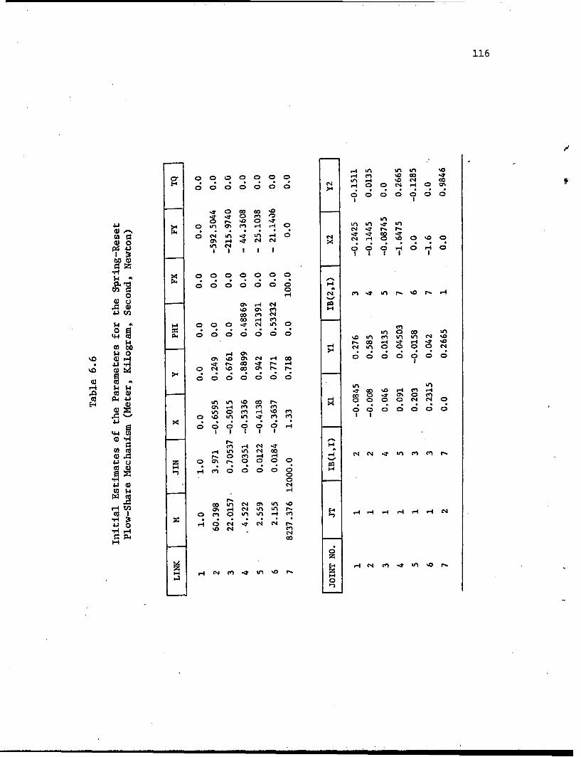
116

0~~L 0 0 0 0 0%

0A ,4 IT F- r

0 0 0 0 0 k-4 00. %n r-4 0T 00

-l; inr0 r -

C) NO 4 0% en H ~ -

00 c-4 mA7 it.40- ~00 n 0 co 0n

0% 0 0 0 0 0 0 0C

0 %0 N

c4 .- M

0 0 0 en c-i %D

p4-4

O~0 0' C-eq.-4 cm 0 0 0 0 0 0 0

0% r4 Cc -n r-. ICo. 1 ~~0 c-i '0 cc o'M r- r-4 r 4 r 4 -

9:0 -4 cc ' .I c' -

c~ ~~4J C4 -n 0'T 0 V'H3 r.4 u4 cn 0cc r

117

*N 0 0 0 0 00.I -

n 00000

cv,

1-4 r4 r-. r-I Wc c'.0 "a Lfl O q H

0. '.0 en L Ltn

u uY) r-. r- 0" a%

4.J4

0 0. 0 0 0 0

~C4 OH - 8 HO C

00H 00 0 000C

H) C) 0

-q r- u 0I

600

En HI~

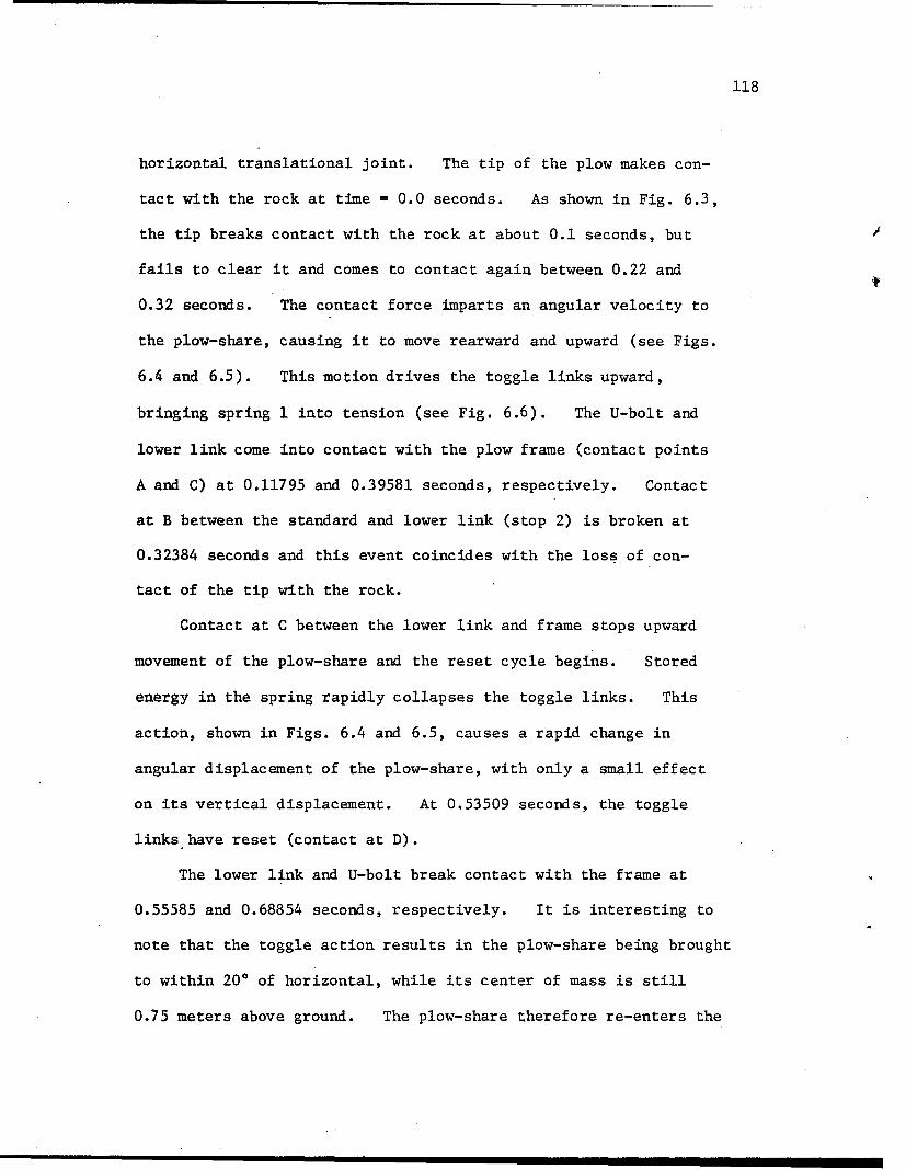
118

horizontal translational joint. The tip of the plow makes con-

tact with the rock at time = 0.0 seconds. As shown in Fig. 6.3,

the tip breaks contact with the rock at about 0.1 seconds, but

fails to clear it and comes to contact again between 0.22 and

0.32 seconds. The contact force imparts an angular velocity to

the plow-share, causing it to move rearward and upward (see Figs.

6.4 and 6.5). This motion drives the toggle links upward,

bringing spring 1 into tension (see Fig. 6.6). The U-bolt and

lower link come into contact with the plow frame (contact points

A and C) at 0.11795 and 0.39581 seconds, respectively. Contact

at B between the standard and lower link (stop 2) is broken at

0.32384 seconds and this event coincides with the loss of con-

tact of the tip with the rock.

Contact at C between the lower link and frame stops upward

movement of the plow-share and the reset cycle begins. Stored

energy in the spring rapidly collapses the toggle links. This

action, shown in Figs. 6.4 and 6.5, causes a rapid change in

angular displacement of the plow-share, with only a small effect

on its vertical displacement. At 0.53509 seconds, the toggle

links have reset (contact at D).

The lower link and U-bolt break contact with the frame at

0.55585 and 0.68854 seconds, respectively. It is interesting to

note that the toggle action results in the plow-share being brought

to within 20' of horizontal, while its center of mass is still

0.75 meters above ground. The plow-share therefore re-enters the

119

0.0

C33

!i 060En

44

0*0 WO000

SNOMM]j, 0NOi):ý

120

,--

P4

C u

4J0

tau

in

(1%

ZOV1 G'N•NVUoi 0

Ill I I i i I I I I I I I I I

121

0

a 3

tom

0ý0 20- 9*- altSNUIOo 4.1O*OI

122

a- '90

C3

E-4

000

ot4-H

9 P:4

(2 OX) SOIMI 'NOSN'0

123

is0"E:

0

V 0

CA U

01001~~~ a 0 lg Oo *

SNOIM3 NO103

124

TIME= 0. t00 TIME= 0.232

TIME= 0.125 TIME= 0.325

Figure 6.8 VERSATEC Plots (Snap-shot pictures) of thePlow-Share Mechanism at Selected Time Instants.

125

44

'I0

"I0U,

U,)

aj

126

I-r.

0

cmU

cmc

a, $

C0

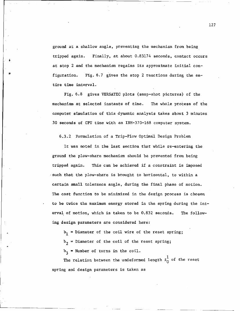
127

ground at a shallow angle, preventing the mechanism from being

tripped again. Finally, at about 0.83174 seconds, contact occurs

at stop 2 and the mechanism regains its approximate initial con-

A figuration. Fig. 6.7 gives the stop 2 reactions during the en-

tire time interval.

Fig. 6.8 gives VERSATEC plots (snap-shot pictures) of the

mechanism at selected instants of time. The whole process of the

computer simulation of this dynamic analysis takes about 3 minutes

30 seconds of CPU time with an IBM-370-168 computer system.

6.3.2 Formulation of a Trip-Plow Optimal Design Problem

It was noted in the last section that while re-entering the

ground the plow-share mechanism should be prevented from being

tripped again. This can be achieved if a constraint is imposed

-such that the plow-share is brought to horizontal, to within a

certain small tolerance angle, during the final phase of motion.

The cost function to be minimized in the design process is chosen

to be twice the maximum energy stored in the spring during the int-

erval of motion, which is taken to be 0.832 seconds. The follow-

ing design parameters are considered here:

b = Diameter of the coil wire of the reset spring;

b2 = Diameter of the coil of the reset spring;

b3 = Number of turns in the coil.

The relation between the undeformed length k0 o the reset

spring and design parameters is taken as

128

1 b + 0.56604 x 10- 2 (6.12)0 b1b3

It should be observed here that since the undeformed lengthof the reset spring depends on b and b is automatically a

1 3

design parameter.

With the notations of Chapters II and III, the optimal design

problem is stated as follows: Minimize

max K 1 )2 (6.13)0<t<0.832

where [72] 1 Gb4

K1=46 3b , G being shear modulus, (6.14)83b2 b3

subject to the equations of motion, Eq. (2.33), the equations of

constraints on motion, Eq. (2.35), the spring-damper relations,

Eqs. (2.36) and (6.11), initial conditions of the form of Eqs. (3.4)

and (3.5), the functional constraint

- ý2 - 0.174533 < 0 , 0.75 < t < 0.832 (6.15)

and the design parameter constraints

bL < b. < bU , i=1,2,3 (6.16)i -- I --

For the functional constraint Eq. (6.15), the maximum allowable

inclination of the plow-share during the interval 0.75 < t < 0.832

of re-entering phase has been taken to be 100.

As in the case of the slider-crank mechanism, with similar

129

notations, the problem can be reformulated as: Minimize

= = b4 (6.17)

subject to-Eqs. (2.33), (2.35)-, (2.36), (6.11), (3.4), and (3.5),

the constraints

-- f2 - 0.174533> > dt = 0 (6.18)J02

0O.832 G b

4

•2 -1< - 1(2- k ) - b4 > dt =0 (6.19)2 0 8b3 b3

2 3

and the design parameter constraint of Eq. (6.16).

In Eq. (6.18) the symbol <<H >> has the following. meaning:

0 for 0 < t <t 1 = 0.75 and for H < 0,

<<H>> (6.20)

H2 , for H > 0

Since the transient analysis itself is extremely complex for this

mechanism, only one regular functional constraint has been consid-

ered. However, additional constraints can be treated.

6.3.3 Modifications in Sensitivity Analysis Due toNon Standard Elements

Owing to the inclusion of nonstandard equations, Eq. (6.11),

in the set of spring-damper relations, some modifications are re-

quired in the sensitivity analysis. The calculations and program-

ming for the additional elements in NPOSR, NPOSC, and G vectors

and the right-hand sides are routinely [7,14] done through the

130

subroutines USET, USOLV1, USOLV2, and USOLV3 together with another

set of subroutines LSPTRS, LSSLV1, LSSLV2, and LSSLV3 (see Chapter

V). The solution vector of (K.i.Ci.) of Eq. (6.11) is included

in the extended vector _£ and the corresponding I matrix of Eq.

(2.38) becomes

0 0

1 0

0

0

0 0

1 0

0E- 0 (6.21)

.j(4s x 4s)

0

0

0 (4s+ NSDV)

x (4s + NSDV)

where NSDV is twice the number of nonlinear spring-damper pairs.

For the sensitivity analysis, necessary modifications are per-

formed in subroutine SOlNEW for calculation of the right-hand sides

/

of the adjoint equations and additional calculations for the values

of 3 are done in DLDFB. Necessary adjustements for the dimensions

of the variable DZIDB are also made. It should be remarked here

131

that DLDFB is called after the call of INTERP, so that the values

in DLDFB are calculated with the interpolated values of the sol-

ution variables.

6.3.4 Numerical Results (AdjointAnalysis and Optimization)

In carrying out the optimal design algorithm, a design re-

duction ratio of 1% is used to compute the step-size in the first

L U -2iteration. The bounds b and b are taken to be [0.2x 10

-1 1 T [O 1x1 O ~l 2]T,O.lxlO , 0.8x1 I] and [0.1xl0-, 0.1, 0.14xi02]T, respect-

ively. The initial estimate bI (including artificial design para-

meter) is taken as [0.56604x10 2 , 0.181361xi0-, O.1xl02

0.16747l 1xi04]. The shear modulus G has been taken to be

1.86x 1010 N/m 2 . The static analysis and static sensitivity anal-

ysis results are given in Table 6.7 and Table 6.8.

It is interesting to note that in the first iteration, all

convergence criteria are satisfied with 116b511 = 0.6209x 10-3

and 116bb211 = 0.2132x10-3 and the final optimum results are given

in Table 6.9.

In order to treat the problem in a different way, the first

functional constraint is redefined such that the tip of the plow-

share remains at least 2" = 0.0508 m. above the ground level dur-

ing a certain interval in the final phase of motion. This time

interval is taken to be [0.6, 0.832]. The corresponding functional

constraint then becomes:

1 - <<H>> dt = 0 (6.22)

132

-q -IT-n

-% Ln a, e -

Hn e'J Ln C4

r, r-, H, Ln Ho t 'i L

0 C-I 4 ' 4 rz H 90_ _ _ _ _ _

0H

S0 ,o r-. 0 in

ON H- a0 Ou a~ %,0na0 -C4 '0 I., -I. r- 00~- ~ U ' ~ '400 00 000 .T T' ~aC .r

-H cn T~ c

w~ ~ ~ C'00 ar 0ý T T

Hn On rs '0 n 0ý '4P- 0- m, 04 %0 %0 ~ mc

0 0 0 0 H4 I - 0 0 0L

cn~

rnH

* 0 . '0 c~, r- r '0 -F4

'0 r~~o a -~ ~ -~-~ a0z

'-.4~~E- H -4 Ln "D *I ' ' t .O~

H

.1-MIT n .

133

C'4

I I

x '00 .q00

r- ~ z i 0 m~ 000 n

CD LO 0

000 0

00

0 0

-H cq , M ~ zr n \.

134

-4 0

to 10114 ý-4

tn "

-44 -4. .4 -4

0 .-i 0 -~0 0 00 at t U

NDo r --

r4 -t %

Un '0, 0%vi . 7 O 9 I- t 00 NO

00 co 0~t a0 00 N 00 0

14~~- m-4-40 0 LM 4n

14 %4 14N

en C1 In 0%0% r4 at '0 0

'0 n Cl 000 00 00

4' 0* .01 .D .4 r*

0.40 N 00 0IrS I

ý4 0 1.4

a) N. C4%0 0

%aa '0Un

0c ~ m 000 ~. O O O 0%0ON

I co 0000 100 % 0 0 0

0 40 00 000 IT 0%0

4J .n .. ?C 1 00 01

Cd cn 10 .?

10 'o -.T.

0 N '0 r- N I

-4 0% '0 0o en 0' 10 U, 00 N r '0 r- 0n.L

00 '000 '0 '0 -00 4 0% 0% 0C-4 1

U) -4 -4

0 04 0 I-f 0 -

0 C. 0 10 V

0% %D C4 0% 0 AA e 0 . 0

N. t-4 In 0T 0% enkn 0 C 0000-40 N!aý 0000

.t 0i .~ ..

C; C3.0. 0 10 0 0 oN r '

o. -4 4c ~

13.5

N C410 1

14-4 0 a

N 0

0o 0IT0Q 0 0 0 0

10 10 10-4 4 -4

0N (I ;r..

0 COO '

144

104

0 00 44v 04 0 0 0

1.4 00

-404-

C14 10

E4 o la

Ln inv0% 0 co

to N .

-4 -4 -44

cn N

0 0 la N -

Ln 0 o %D xa 10 -It 0

m Ln 10

0- 0 4M * 0 0 04 0

136

where

H H 0.2508 - [Y(2)+XFI(6)*DSIN(PHI(2))

+ YF1(6)*D COS (PHI(2))] (6.23)

and 0•f, for 0 < t < t = 0.6 and for H < 0<<H>> = H (6.24)2,for H>• 0

The computer variables used in Eq. (6.23) are explained in Chapter

V.

For this case a design reduction ratio of 5% is used and the

bounds bL and bU are kept unchanged. The initial estimate BI is

taken as [0.566x10-2 , 0.181361 x101, 0.1x102, 0. 1 67 4 7 1 x 1041T.

In this case, optimum results are obtained in the first iteration,

with 11~b0j = 0.0 and I16b21, = 0.2011x10-4. The final results

are given in Table 6.10.

It should be remarked here that although the results in Tables

6.9 and 6.10 are quite similar, the results of Table 6.9 are prefer-

able, because the constraint on inclination of the plow-share is

more important than the one on the height of the plow-share tip.

In order to deal with a more meaningful problem of iterative

optimal design, the maximum inclination of the plow-share during

the interval 0.6 < t < 0.832 of the re-entering phase is reduced to

0.017453 radians. Then Eqs. (6.15) and (6.18) reduce to

- ý2 - 0.017453 < 0 , 0.6 < t <,0.832 (6.25)

and

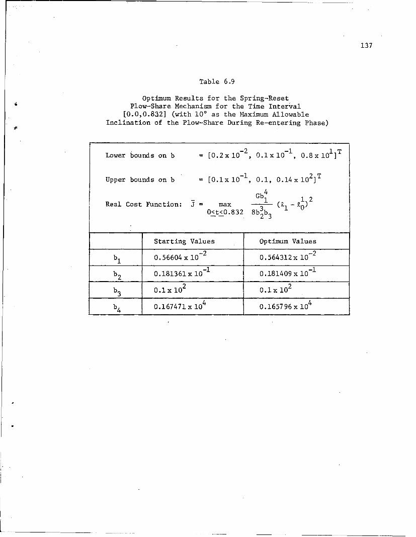
137

Table 6.9

Optimum Results for the Spring-ResetPlow-Share Mechanism for the Time Interval

[0.0,0.8a2] (with 100 as the Maximum AllowableInclination of the Plow-Share During Re-entering Phase)

boudsonb 0. -.2 -1 1 TLower bounds on b = [0.2x10-, 0.lxlO , 0.8x101i

Upper bounds on b =[.lx 10-1, 0.1, 0. 1 4 x102]T

Gb14 1 2Real Cost Function: = max b z - 0)0<t<0.832 83b 3 (b 1 0

Starting Values Optimum Values

b 0.56604 x 10- 2 0.564312x 10-2

b2 0.181361 x 10-1 0.181409 x 10-1

b3 0.1x102 0.1x 10 2

b4 0.167471x 10 4 0.165796 x 10 4

138

Table 6.10

Optimum Results for the Spring-ResetPlow-Share Mechanism with

Modified Functional Constraint

G

Real Cost Function: =_max 1 b12 (k - 0)

O<t<O.832 8 b 3 b 1 02 3

Lower bounds on b = [0.2x10 , 0.1xl0-, 0.8x101]

Upper bounds on b = [O.1xlO- , 0.1, 0.14x i02]T

Starting Values Optimum Values

b1 0.566 x 10- 2 0.567958 x 10-2

b2 0.181361 x 10-1 0.181315 x 10-1

b3 0.1x 10 2 0.1x 10 2

b4 0.167471x 10 4 0.167471x 10 4

(app.)

139

0.832

1 << -2 0.017453 >> dt 0 (6.26)

respectively. All other equations in the set of Eqs. (6.12) to

(6.20) remain unaltered.

For this case a design reduction ratio of 0.25% is used and

the bounds bL and bU are kept unchanged. The initial estimate

b is taken as [0.56604x10 2 , 0.181361xlO1 , 01x102

0.1 6 0 0 0 x 104]T. After three iterations the convergence criteria

are satisfied and the optimum results are reached. Tables 6.11

and 6.12 present the pertinent numerical results of interest for

various iterations.

140

%01 %ofo %0, 1~en C, en0 m 0

J 0 0o

oq co go00 MO14

$4s 0 C;% l1-40 1ON 0%0 0%0

P4 co C4 00- .- 4 co -f

.0C4 -4 C-4

P4 to.- ,0 001 c 10C04 ____4_r--______

1- co - c

41 C'4 ý4

- 0 10 -4 103~I C*-C% .U, c .e4

CO 03 X,. 1!' Or-. or03 03 ~ -4 _ _ _ __0_ _

Ct-4 0 - C4 0! 'o1 I4'041C;I - 0,0 .0 w-.0Cd Cfl ý4 C - . -4 -I Cq J. C4 1-4

.0 1O~- 0 0 0o

o m3

44 U, 000 O

IT j 1. CJ-4 .- C'4E- -4 I 0 a0 '0 aIT0oo - :1c 0 00 0o

-440-r-4 r-

4J~z CD 'T -I 0 0%u- 0a C-4 ogojo'-,

*n 10-4 LM- U,-4n03 ,4 1- 1- '-4

LW 0-4 0

4~i 0I- a .1- B.

-4 C-0

~0 1,* J 0 0 0% i

1.4cc *1-4 c

141

,a 10 0 0

cq

10

< Iý

' co C' 4 C'30 -4 F-4

ýa~e' P4 YN -1Cd~I 10 CA

'0 0d I I

0) 00W4

F- 4 a)00D 0 0N

< 'i C'IC'

0 O

II H 4 r

142

CHAPTER VII

CONCLUSIONS AND RECOMMENDATIONS

In this research, a systematic and unified theory for obtaining

a corresponding computer program for dynamic analysis, static sensiti-

vity analysis, general design sensitivity analysis, and optimal design

of large scale constrained dynamic systems has been developed and demon-

strated. Constrained mechanical systems with continuous motion, as in

the case of the slider-crank mechanism of Chapter VI, and those with

intermittent motion, as in the case of the plow-share mechanism dis-

cussed in Chapter VI, are handled with ease. The stiff integration

(Gear) algorithm [6,21 and sparse matrix techniques [6,10,60,61,621 have

been successfully employed in the DADS program that is presented here.

The DADS program is presently configured for two-dimensional systems,

but the extension to three-dimensional systems is theoretically

straightforward.

It was noted in Chapter V that the DADS computer program is

capable of dealing with mechanical systems with discrete rigid

bodies only. If necessary, some amount of deformability in special

elements of mechanisms can be introduced, with the help of additional

spring-damper pairs. Otherwise, finite element techniques are to

be introduced for the deformable elements and the Jacobian should

be constructed accordingly. Then all types of analyses treated

here can be performed in a routine manner. However,

143

for average-shaped mechanisms, introduction of deformability through

spring-dampers is recommended. For structural problems, when the

forcing functions depend on time and on solution variables, the

conventional way of obtaining global solutions through modal analysis

and Duhamel Integrals [54] fails and the techniques employed in this

development may be employed. For structures such as automobiles,

where finite element techniques are to be used for chassis and frames,

in conjunction with the motion of rigid body mechanisms in the sus-

pension systems, sparse matrix techniques and stiff integration

(Gear) algorithms are indispensible.

Looking back into the details of the DADS computer program, it

is the opinion of the author that some modifications and refine-

ments, particularly in the field of numerical integration, are nec-

essary to make it more efficient. Among other refinements, the

following are under active consideration:

(1) Storage of the values of only those solution variables and

related data in a disk in transient analysis, that are to be

used in adjoint analysis. This then becomes a problem-

dependent affair.

(2) Allotment of only one disk for storing the solution data set

of the adjoint equations corresponding to all violated con-

straints in the sensitivity analysis.

144

APPENDIX

MATHEMATICAL RELATIONS USED IN THE SUBROUTINESRELATE, DGDBZ, ADLDZ, AND DLDFB

FOR THE EXAMPLE PROBLEMS

In the following, symbols of Chapter II and V and data given in

Chapter VI have been used.

The Slider-Crank Mechanism

Subroutine RELATE:

From Fig. 2.5 and the initial data (Table 6.1), one obtains

1 2KM =b b3 33 3

K b=

YFl(1) = b2

YF2(1) = b2 - 0.5

X1(3) = b 3

X2(2) = -b 3

X(3) = b 3 cos cl3

X(4) = 2.DO x X(3)

145

Subroutine DGDBZ:

From Eqs. (6.6) to (6.9)

DGDB(l) = DGDB(2) = DGDB(3) = DGDB(4) = 0

for all the four functional constraints. Only for the cost function

DGDB(4) = 1.0 and DGDB(I) = 0, I 1,2,3

Also for the fourth constraint, the only nonzero component for DGDZM

is given by

DGDZM(9) = 1.0

Subroutine ADLDZ:

From Eq. (6.6), one obtains for the first constraint (since p 2 is

the 26-th solution variable),

DLDZ(26) = -Al*(l.DO + DSIGN(l.DO,Al))/10.DO

where

A1- ( 21. + 1.D0 + 6

lO1.DO

e being the E-active constant. All other compontnets are zero.

D after decimal point indicates double precision. The function

DSIGN(al,a2), al,a 2 being the arguments,is defined as follows:

DSIGN(al,a 2) = jall sgn(a 2 )

where

146

1 for a2 > 0

sgn(a 2 ) 1 for a2 = 0

-1 for a 2 < 0

From Eq. (6.7), one obtains for the second constraint the only nonzero

component as

DLDZ(26) = Al*(l.DO + DSIGN(1.DO,A1))/10.D0

where

A1 = I.D0+ e.10.D0

From Eq. (6.8), one obtains for the third constraint the only nonzero

component as

DLDZ(33) = 2.DO*b *Al*A2*(l.DO+ DSIGN(l.DO,A2))/b 4

where

Al = 9 k0

1 0

b* (Al)2

A2 -1 - l.DO +b 4

From Eq. (6.9) all components of DLDZ are zero for the fourth con-

straint.

Subroutine DLDFB:

The nonzero components of DLDB, DFDB, DPHDB, and DZIDB are given

by the following relations. For the third constraint

147

DLDB(l) = (Al) 2*A2*(l.DO + DSIGN(l.DO,A2))/b 4

DLDB(4) = -A2*(l.DO + DSIGN(l.DO,A2))*bI*(Al) 2 /(b 4 )2

where

Al =.1 0

b * (Al)2

A2 b -1.D0 + Eb4

From the equations of motion, one obtains

DFDB(15,3) = -(P13 + P 5) sin 43 + (P4 + C6 Cos 43

1 1 in@DFDB(21,2) = FX cos 4 + F sin

1 1 sniDFDB(3,2) = -F1 cos 4) - F six 1 y n4 1

From the equations of constraints, one obtains

DPHDB(3,3) = cos 43 = DPHDB(5,3)

DPHDB(4,3) - sin 43 = DPHDB(6,3)

From the spring-damper relations, one obtains

10

DZIDB(3,1) = 1 xi

1 01

148

[XI*(-sin i + sin + YI*(cos - cos ¢4)]DZIDB (i,2) = 42

[(XI) + (YI) 2]1/2

DZIDB(3,2) = b1 1 -0 * (-sin 1 + sin ¢4)

0 1

DZIDB(4,2) = b1 1 * (Cos £i - Cos 4

where

XI =XGI - XG2, YI =YGI - YG2

XG1 XF1(1) * cos - YFl(1) * sin + X(1)

YGl XFl(1) * sin i + YF1(l) * cos + Y(1)

XG2 = XF2(1) * cos ¢4 - YF2(l) * sin 4 + X(4)

YG2 XF2(1) * sin 4)4 + YF2(l) * cos 4 + Y(4)

The Plow-Share Mechanism

(with re-entering angle of 0.0174533 radians)

Subroutine RELATE:

From the initial data and definition of the design parameters

(Chapter VI), one obtains (see Eqs. (6.14) and (6.12),

b4

K1 = 23.25 x 108 x 1

b 3b 3b3b2

149

k 1 b b + 0.56604 x 10-20 1 3

Subroutine DGDBZ:

In this case the only nonzero component of DGDB is given by

DGDB(4) = 1.0

for the cost functional only.

All the components of DGDZM are zero.

Subroutine ADLDZ:

The nonzero components of DLDZ are given by the following. From

Eq. (6.18), one obtains for the first constraint,

DLDZ(12) = -Al x (l.D0 + DSIGN(l.DO,Al)) , for t > 0.6DO

where

Al = -2 - 0.0174533D0 + c

From Eq. (6.19), one obtains for the second constraint

DDZ(57) = 2.D0 * K1 * Al * A2 * (l.DO + D SIGN(l.DO,A2))/b 4

where

Al = k £11 0

A 1 2 i-£

K 1 (Al)-A2 = b 1.DO E

150

Subroutine DLDFB:

The nonzero components of DLDB, DFDB, DPHDB, and DZIDB are given

by the following relations. From Eq. (6.14)13

9K = 93.D08 * b1---

3 2

1K b14

-- = -69.75D08 * 1

4

•b2 3 b2

K1 b14

3K = _-23.25D08 19b 3 b2 b3

3 2

Then for the second constraint

DLDB(l) = A3 * ((Al) * -KI 2.DO * K * Al * )/bab1

DLDB(2) = A3 * (Al) * -KK

3b2

DLDB(3) = A3 * ((Al) *2 -K - 2.DO * K * Al * b )Ib3b3 1 4

DLDB(4) = -( * A3 * (Al)2

2

w4

where

151

1A l = Yi -1 k0

K1* (Al) 2

A2 K - l.D0 +

A3 A2 * (1.DO + DSIGN(1.DO,A2))

From the relations corresponding to the first-spring-damper pair, one

obtains

DZIDB(3,1) = DLU *- - DL3 * bab 1 3

1DZIDB(3,2) = DLU * a

ab2

DZIDB(3,3) = DLU * - DL3 * bab11

K1

DZIDB(4,1) = DL2 * -a- - DL4 * bDb 1 3

DZIDB(4,2) = DL2 * a3b 2

DZIDB(4,3) = DL2 * - DL4 *bwb3

where

152

1

DL1 = 12 0 Y

DL2 = K1~ * Y

1 1I

XI=XG1 -XG2 , YI=YG1-YG2

XG1 =XF1(1) * cos P 4 YF1(1) * sin ý + X4

YG1 = XF1(1) * sin 4+ YF1 (1) * cos 4+ 4

XG2 = XF2(1) * cos 6- YF2(1) * si + X 6

YG2= XF2(1) *sin 6+ YF2(1) *cos 6 + Y6

153

REFERENCES

1. Haug, E.J., Jr., "Computer Aided Design of MechanicalSystems", Army Materiel Command Engineering DesignHandbook, AMCP 706-192, 1973.

2. Gear, C.W., "Numerical Initial Value Problems in OrdinaryDifferential Equations", Prentice-Hall, Inc., 1971.

3. Lambert, J.D., "Computational Methods in Ordinary Diff-erential Equations", John Wiley & Sons, New York, 1973.

4. Lapidus, L., and Seinfeld, J.H., "Numerical Solution ofOrdinary Differential Equations", Academic Press, NewYork, 1971.

5. Willoughby, R.A., "Stiff Differential Systems", PlenumPress, New York and London, 1974.

6. Chua, L.O., and Lin, P.M., "Computer-Aided Analysis ofElectronic Circuits", Prentice-Hall, Inc., Englewood Cliffs,N.J., 1975.

7. Orlandea, N., "Node Analogous, Sparsity-Oriented Methods forSimulation of Mechanical Dynamic Systems", Ph.D. Thesis,University of Michigan, Ann Arbor, Mich., 1973.

8. Orlandea, N., Chace, M.A., and Calahan, D.A., " A Sparsity-Oriented Approach to the Dynamic Analysis and Design of Mech-anical Systems, Parts I and II", Journal of Engineering forIndustry, ASME paper No. 76-DET-19/20, 1976.

9. Chace, M.A., and Sheth, P.N., "Adaptation of Computer Tech-niques to the Design of Mechanical Dynamic Machinery", ASMEpaper 73-DET-58, ASME Meeting, Cincinnati, Ohio, September9-12, 1973.

10. Calahan, D.A., "Computer-Aided Network Design, 2nd ed.,McGraw-Hill, New York, 1972.

11. Carnaham, B., Luther, H.A., and Wilkes, J.O., "AppliedNumerical Methods", Wiley, New York, 1969.

12. Calahan, D.A., Grapes, T.E., and Korybalski, M.E., PrivateCommunications.

154

13. ASTAP (Advanced Statistical Analysis Program), developed byIBM System Products Division, East Fishkill, New York,April 20, 1973.

14. Wehage, R.A., "ADAMS 2-D Automatic Dynamic Analysis of Mech-anical Systems - Two Dimensional", M.S. Report, Iowa StateUniversity, Ames, Iowa,

15. Sheth, P.N., "A Digital Computer-Based Simulation Procedurefor Multiple Degree of Freedom Mechanical Systems withGeometric Constraints", Ph.D. Thesis, University of Wisconsin,Madison, Wis., 1972.

16. Sheth, P.N., and Uicker, J.A., Jr., "IMP (Integrated MechanismsProgram): A Computer-Aided Design Analysis System for Mech-anisms and Linkages", Trans., ASME 94, Ser. B, J. Eng.Indust., 454-464, 1972.

17. Chace, M.A., and Angell, J.C., "User's Guide to DRAM(Dynamic Response of Articulated Machinery)", Design Engin-eering Computer Aids Laboratory, Department of MechanicalEngineering, University of Michigan, 1973.

18. Chace, M.A., and Bayazitoglu, Y.O., "Development and Applic-ation of a Generalized D'Alembert Force for MultifreedomMechanical Systems", J. Eng. Indust., 317-327, 1971.

19. Dix, R.C., and Lehman, T.J., "Simulation of the Dynamics ofMachinery", J. Eng. Indust., Trans. ASME, Ser. B, 94,433-438, 1972.

20. Andrews, G.C., and Kesavan, H.K., "The Vector Network Model:A New Approach to Vector Dynamics", Mechanism and MachineTheory, 10 (1), 57-75, 1975.

21. Paul, B., and Krajcinovic, D., "Computer Analysis of Machineswith Planar Motion - 2. Dynamics", J. Appl. Mech. 37,703-712, Trans. ASME 92, Ser. E, 1970.

22. Paul, B., "Analytical Dynamics of Mechanisms - A ComputerOriented Overview", Mechanism and Machine Theory, Vol. 10,481-507, 1975.

23. Seireg, A., "A Survey of Optimization of Mechanical Design",J. Eng. Indust., Vol. 94, Trans. ASME, 495-499, 1972.

155

24. Haug, E.J., Jr., and Arora, J.S., "Optimal Mechanical DesignTechniques Based on Optimal Control Methods", Proceedings ofthe First ASME Design Technology Transer Conference, 65-73,October 1974.

25. Sevin, E., and Pilkey, W., "Computational Approaches to theMin-Max Response of Dynamic Systems with Incompletely PrescribedInput Functions", J. Appl. Mech., Vol. 34, Trans., ASME, 87-90,March 1967.

26. Fiacco, A.V., and McCormick, G.P., "The Sequential Uncon-strained Minimization Technique for Nonlinear Programming, aPrimal Dual Method", Management Science, Vo. 10, pp.360-366,1964.

27. Sevin, E., Pilkey, W.D., and Kalinowski, A.J., "OptimumPerformance Bounds and Synthesis of Dynamic Systems",Computational Approaches in Applied Mechanics, ASME, New York,107-132, 1970.

28. Sevin, E., and Pilkey, W.D., "Optimum Shock and VibrationIsolation", The Shock and Vibration Information Center, UnitedStates Department of Defense, 1971.

29. Bellman, R., and Dreyfus, S., "Applied Dynamic Programming",Princeton University Press, Princeton, N.J., 1962.

30. Brock, J.E., "A note on the Damped Vibration Absorber", J.Appl. Mech., Vol. 13, Trans. ASME, A-284, 1946.

31. Den Hartog, J.P., "Mechanical Vibrations", McGraw-Hill BookCompany Inc., New York, 1956.

32. Hamad, B.M., "Optimum Design of Vibratory Systems', Ph.D.Thesis, University of Wisconsin, 1968.

33. Arora, J.S., Rim, K., and Kwak, B.M., "Optimum Design ofDamped Vibration Absorber", Technical Report No. 7, Departmentof Mechanics and Hydraulics, College of Engineering, Universityof Iowa, Iowa City, Iowa, July 1973.

34. Afimiwala, K.A., and Mayne, R.W., "Optimum Design of anImpact Absorber", J. Eng. Indust., Vol. 96, Trans. ASME,124-130, February 1974.

35. Willmert, K.D., and Fox, R.L., "Optimum Design of a LinearMulti-Degree of Freedom Shock Isolation System", J. Eng.Indust., Vol. 94, Trans. ASME, 465-47;. May 1972.

156

36. McMunn, J., "Multi-Parameter Optimum Damping in LinearDynamical Systems", Ph.D. Thesis, University of Minnesota,1967.

37. Kwak, B.M., "Parametric Optimal Design", Ph.D. Thesis,University of Iowa, December 1974.

38. Hsiao, M.H., "Mechanical Design Optimization for TransientDynamic Response", Ph.D. Thesis, University of Iowa,May 1976.

39. Haug, E.J., Jr., and Arora, J.S., "A State-Space Method forOptimization of Weapon System Dynamics", Proceedings, FirstConference on Dynamics of Precision Gun Weapons, Rock Island,Illinois, January 1977.

40. Huang, R.C., "Optimal Design of Mechanical Systems withIntermittent Motion", Ph.D. Thesis, University of Iowa,May 1976.

41. Huang, R.C., Haug, E.J., Jr., and Andrews, J.G., "OptimalDesign of Mechanical Systems with Intermittent Motion,Technical Report No. 24, Division of Materials Engineering,University of Iowa, Iowa City, Iowa, 1976.

42. Chua, L.O., "Introduction to Nonlinear Network Theory",McGraw-Hill Book Company, New York, 1969.

43. Hilderbrand, F.B., "Introduction to Numerical Analysis",McGraw-Hill Book Company, New York, 1956.

44. Conte, S.D., and De Boor, Carl, "Elementary NumericalAnalysis - An Algorithmic Approach", McGraw-Hill Book Company,New York, 1972.

45. Ralston, A., "A First Course in Numerical Analysis", McGraw-Hill Book Company, New York, 1965.

46. Gear, C.W., "Simultaneous Numerical Solution of Differential -Algebraic Equations", Trans. Circuit Theory, Vol. CT-18, No. 1,89-95, January 1971.

47. Grenin, Y., "A New Approach to the Synthesis of StifflyStable Linear Multistep Formulas", IEEE Trans. Circuit Theory,352-360, July 1973.

157

48. Gear, C.W., "The Automatic Integration of Stiff OrdinaryDifferential Equations", Information Processing 68,A.J.H. Morrell, Ed., North Holland Publishing Company,Amsterdam, The Netherlands, 187-193, 1969.

49. Hachtel, G.D., Brayton, R.K., and Gustavson, F.G., "TheSparse Tableau Approach to Network Analysis and Design",Trans. Circuit Theory, Vol. CT-18, No. 1, 101-113, January1971.

50. Orlandea, N., Chace, M.A., and Calahan, D.A., "SparsityOriented Methods for Simulation of Mechanical Dynamic Systems",Proceedings of the sixth annual Princeton Conference on Inform-ation Sciences and Systems, Department of Electrical Engineering,Princeton University, Princeton, N.J., 32-36, 1972.

51. Calahan, D.A., and Orlandea, N., "A Program for the Analysisand Design of General Dynamic Mechanical Systems", AFIPSConference Proceedings, Vol. 41, Part II, Fall Joint ComputerConference, Anaheim, California, 885-888, 1972.

52. Strang, W.G., and Fix, G.J., "An Analysis of the FiniteElement Method", Prentice-Hall Book Company, Englewood Cliffs,N.J., 1973.

53. Zienkiewicz, O.C., "The Finite Element Method in Structuraland Continuum Mechanics", McGraw-Hill Book Company, New York,1967.

54. Clough, R.W., and Penzien, J., "Dynamics of Structures",McGraw-Hill Book Company, New York, 1975.

55. Crout, P.D., "A Short Method for Evaluating Determinants andSolving Systems of Linear Equations with Real or ComplexCoefficients", AIEE Trans., Vol. 69, 1235-1241, 1941.

56. Calahan, D.A., Grapes,.T.E., Donahey, J., and Orlandea, N.,"Description of a Sparse Matrix Compiler with Applications",AFOSR-TR-71-2676, October 11, 1971.

57. Berry, R.D., "An Optimum Ordering of Electronic CircuitEquations for a Sparse Matrix Solution", IEEE Trans. CircuitTheory, Vol. CT-18, 40-50, January 1971.

58. Tinney, W.F., and Walker, J.W., "Direct Solutions of SparseNetwork Equations by Optimally Ordered Triangular Factorization",Proc. IEEE, Vol. 55, 1801-1809, November 1967.

158

59. Markowitz, H.M., "The Elimination Form of the Inverse andIts Application to Linear Programming", Management Sci.,Vol. 3, 255-269, 1957.

60. Proceedings, Sparse Matrix Symposium, IBM Rep. RA-l, March1969.

61. IBM System 360 and System 370 Subroutine Library - Mathematics(SL-MATH), No. 5736-XM7, 1971. (Rental Software available fromIBM).

62. Calahan, D.A., Buning, P.G., and Joy, W.N., "VectorizedGeneral Sparsity Algorithms with Backing Store", SystemsEngineering Laboratory (SEL), Report No. 96, University ofMichigan, Ann Arbor, Michigan, January 1977.

63. Haug, E.J., Jr., "Computational Methods in Mechanical SystemDynamics", The University of Iowa, February 1978.

64. Bunch, J.R., and Rose, D.J., "Sparse Matrix Computations",Academic Press Inc., New York, 1976.

65. Tewarson, R.P., "Sparse Matrices", Academic Press Inc., NewYork, 1976.

66. Goldstein, H., "Classical Mechanics", Addison-WesleyPublishing Company Inc., Cambridge, Mass., 1953.

67. Greenwood, D.T., "Classical Dynamics", Prentice-Hall Inc.,Englewood Cliffs, N.J., 1977.

68. Kane, T.R., "Dynamics", Second Edition, Stanford UniversityPress, Palo Alto, California, 1972.

69. Liusternik, L.A., and Sobolev, V.J., "Elements of FunctionalAnalysis", Ungar, New York, 1961.

70. Lanczos, C., "Linear Differential Operators", Van Nostrand,London, 1961.

71. Mischke, C.R., "Elements of Mechanical Analysis", Addison-Wesley Publishing Company, Inc., Massachusetts, 1963.

72. "Mark's Standard Handbook for Mechanical Engineers", Inter-national Student Edition, McGraw-Hill Book Company, New York.

159

73. Businger, P.A., "Monitoring the Numerical Stability ofGaussian Elimination", Numer. Math. 16, 360-361, 1971.

74. Erisman, A.M., and Reid, J.K., "Monitoring the Stabilityof the.Triangular Factorization of a Sparse Matrix",Numer. Math. 22, 183-186, 1974.

DISTRIBUTION LIST

Please notify USATACOM, DRSTA-ZSA, Warren, Michigan 48090, of correctionsand/or changes in address.

Commander (25) Director (01)US Army Tk-Autmv Command Defense Advanced ResearchR&D Center Projects AgencyWarren, MI 48090 1400 Wilson Boulevard

Arlington, VA 22209Superintendent (02)US Military Academy Commander (01)ATTN: Dept of Engineering US Army Combined Arms Combat

Course Director for Developments ActivityAutomotive Engineering ATTN: ATCA-CCC-S

Fort Leavenworth, KA 66027Commander (01)US Army Logistic Center Commander (01)Fort Lee, VA 23801 US Army Mobility Equipment

Research and Development CommandUS Army Research Office (02) ATTN: DRDME-RTP.O. Box 12211 Fort Belvoir, VA 22060ATTN: Dr. F. Schmiedeshoff

Dr. R. Singleton Director (02)Research Triangle Park, NC 27709 US Army Corps of Engineers

Waterways Experiment StationHQ, DA (01) P.O. Box 631ATTN: DAMA-AR Vicksburg, MS 39180

Dr. HerschnerWashington, D.C. 20310 Commander (01)

US Army Materials and MechanicsHQ, DA (01) Research CenterOffice of Dep Chief of Staff ATTN: Mr. Adachifor Rsch, Dev & Acquisition Watertown, MA 02172ATTN: DAMA-AR

Dr. Charles Church Director (03)Washington, D.C. 20310 US Army Corps of Engineers

Waterways Experiment StationHQ, DARCOM P.O. Box 6315001 Eisenhower Ave. ATTN: Mr. NuttallATTN: DRCDE Vicksburg, MS 39180

Dr. R.L. HaleyAlexandria, VA 22333 Director (04)

US Army Cold Regions Research& Engineering LabP.O. Box 282ATTN: Dr. Freitag, Dr. W. HarrisonDr. Liston, LibraryHanover, NH 03755

President (02) Director (02)Army Armor and Engineer Board Defense Documentation CenterFort Knox, KY 40121 Cameron Station

Alexandria, VA 22314Commander (01)US Army Arctic Test Center US Marine Corps (01)APO 409 Mobility & Logistics DivisionSeattle, WA 98733 Development and Ed Command

ATTN: Mr. HicksonCommander (02) Quantico, VA 22134US Army Test & EvaluationCommand Keweenaw Field Station (01)ATTN: AMSTE-BB and AMSTE-TA Keweenaw Research CenterAberdeen Proving Ground, MD Rural Route 121005 P.O. Box 94-D

ATTN: Dr. Sung M. LeeCommander (01) Calumet, MI 49913US Army Armament Researchand Development Command Naval Ship Research & (02)ATTN: Mr. Rubin Dev CenterDover, NJ 07801 Aviation & Surface Effects Dept

Code 161Commander (01) Washington, D.C. 20034US Army Yuma Proving GroundATTN: STEYP-RPT Director (01)Yuma, AZ 85364 National Tillage Machinery Lab

Box 792Commander (01) Auburn, AL 36836US Army Natic LaboratoriesATTN: Technical Library Director (02)Natick, MA 01760 USDA Forest Service Equipment

Development CenterDirector (01) 444 East Bonita AvenueUS Army Human Engineering Lab San Dimes, CA 91773ATTN: Mr. EckelsAberdeen Proving Ground, MD Engineering Societies (01)21005 Library

345 East 47th StreetDirector (02) New York, NY 10017US Army Ballistic Research LabAberdeen Proving Ground, MD Dr. I.R. Erlich (01)21005 Dean for Research

Stevens Institute of TechnologyDirector (02) Castle Point StationUS Army Materiel Systems Hoboken, NJ 07030Analysis AgencyATTN: AMXSY-CMAberdeen Proving Ground, MD21005

Grumman Aerospace Corp (02) CALSPAN Corporation (01)South Oyster Bay Road Box 235ATTN: Dr. L. Karafiath Library

Mr. F. Markow 4455 Benesse StreetM/S A08/35 Buffalo, NY 14221

Bethpage, NY 11714SEM, (01)

Dr. Bruce Liljedahl (01) ForsvaretsforskningsanstaltAgricultural Engineering Dept Avd 2Purdue University Stockholm 80, SwedenLafayette, IN 46207

Mr. Hedwig (02)Mr. H.C. Hodges (01) RU 111/6Nevada Automotive Test Center Ministry of DefenseBox 234 5300 Bonn, GermanyCarson City, NV 89701

Foreign Science & Tech (01)Mr. R.S. Wismer (01) CenterDeere & Company 220 7th Street North EastEngineering Research ATTN: AMXST-GEI3300 River Drive Mr. Tim NixMoline, IL 61265 Charlottesville, VA 22901

Oregon State University (01) General Research Corp (01)Library 7655 Old Springhouse RoadCorvallis, OR 97331 Westgate Research Park

ATTN: Mr. A. ViiluSouthwest Research Inst (01) McLean, VA 221018500 Culebra RoadSan Antonia, TX 78228 Commander (01)

US Army Developmant andFMC Corporation (01) Readiness CommandTechnical Library 5001 Eisenhower Avenue.P.O. Box 1201 ATTN: Dr. R.S. WisemanSan Jose, CA 95108 Alexandria, VA 22333

Mr. J. Appelblatt (01)Director of EngineeringCadillac Gauge CompanyP.O. Box 1027Warren, MI 48090

Chrysler Corporation (02)Mobility Research Laboratory,Defense EngineeringDepartment 6100P.O. Box 751Detroit, MI 48231