I. Anders (ZAMG) andA. Walter (DWD) - CLM-Community - www ... · COSMO/CLM Training Course 2017 4...
68
Evaluation 31.03.2017 Supported by: K.S. Radtke, K. Keuler, A. Will, M. Woldt, G. Georgiewski (BTU) B. Rockel, B. Geyer (HZG) D. Lüthi, S. Kotlarski (ETH) B. Früh, S. Brienen, K. Trusilova, J. Trentmann (DWD) I. Anders (ZAMG) and A. Walter (DWD)
Transcript of I. Anders (ZAMG) andA. Walter (DWD) - CLM-Community - www ... · COSMO/CLM Training Course 2017 4...

Evaluation
31.03.2017
Supported by:K.S. Radtke, K. Keuler, A. Will, M. Woldt, G. Georgiewski (BTU)B. Rockel, B. Geyer (HZG)D. Lüthi, S. Kotlarski (ETH)B. Früh, S. Brienen, K. Trusilova, J. Trentmann (DWD)
I. Anders (ZAMG) and A. Walter (DWD)

Overview
COSMO/CLM Training Course 2017 2
• General aspects on evaluation
• Observations
• Measures and scores
• ETOOL
• Example: Evaluation of cosmo5.0_clm6
General aspects on evaluation

General aspects on evaluation
COSMO/CLM Training Course 2017 4
… some definitions
model (climate): simplified simulation of reality in compliance with physical basic principles, using physical basic equations, approximations and parameterizations.
program: translation of the model onto a computer
verification: the process of determining that a model implementation accurately represent the developer`s conceptual description of the model and to the solution of the model
validation: the process of determining the degree to which a model is an accurate representation of the real world from the perspective of the intended uses of the model
evaluation: rating of a model and the associated program with respect to its accuracy
General aspects on evaluation
COSMO/CLM Training Course 2017 5
What is evaluation?
• assessing the quality of a simulation
• comparing the simulation against a corresponding observation of what actually occurred, or some good estimate of the true outcome
• evaluation can be qualitative ("does it look right?") or quantitative ("how accurate is it?")

General aspects on evaluation
COSMO/CLM Training Course 2017 6
Source: https://public.wmo.int/en/bulletin/predictability-beyond-deterministic-limit
forecast
climate simulation
Evaluation in NWP / climate mode
• NWP – evaluates forecast against observations
– frequently called verification
• climate simulation
– evaluates (re-)analysis driven simulations with observations
General aspects on evaluation
COSMO/CLM Training Course 2017 7
Why evaluate?
simulation is like an experimentgiven: set of conditions .. � hypothesis: certain outcome will occur;experiment is complete when outcome is checked
aim:
• to monitor simulation quality - how accurate are the simulations and are they improving over time?
• to improve simulation quality - the first step toward getting better is discovering what you're doing wrong.
• to compare the quality of different modeling systems - to what extent does one modeling system give better simulations than another, and in what ways is that system better? Why is a specific model configuration better than another?

General aspects on evaluation
COSMO/CLM Training Course 2017 8
consistencydegree to which the simulation corresponds to the modelers best judgment about the situation, based upon his/her knowledge base
qualitydegree to which the simulation corresponds to what actually happened
valuedegree to which the simulation helps a decision maker to realize some incremental economic and/or other benefit
Essay on
What makes a simulation "good"? (A. Murphy 1993)
Three types of „goodness“

Observations

Observations
COSMO/CLM Training Course 2017 10
Station measurements

Observations
COSMO/CLM Training Course 2017 11
Point measurement versus area average
station measurement - gridded observations
precipitation field
measuring site
grid
subgrid scale distribution of
variable
∆x
depending on grid resolution!

Observations
COSMO/CLM Training Course 2017 12
Problems with station measurement
• measurement representative for a point and not the grid cell
• observations suffer from measurement uncertainties
• when looking at longer term statistics instantaneous errors might cancel out (to a certain degree) but do not look at single cases in time (e.g. extreme events)!
• Be aware: in a high-resolution station network: neighboring stations might not have independent information!
� if possible: use area average!

Observations
COSMO/CLM Training Course 2017 13
Uncertainties in station measurements due to:
• changes in the location
• changes in the measuring instruments (e.g. instrument type or measuring method)
• changes in the stations surrounding
• calibration
• slightly decreased quality
• any change without documentation
• changes in thresholds (sunshine)
• wind influence (for precipitation)
• icing of the instruments
• mountain station (exposure, difficult to reach, representability)
• human error (missing motivation, missing skill, reading error, error while digitalization)
• changes in recording times
• influence of animals
• vandalism

Observations
COSMO/CLM Training Course 2017 14
after homogenisation
original time series
Trends in maximum temperature per year

Observations
COSMO/CLM Training Course 2017 15
Problems with gridded observations
• uncertainties introduced by interpolation method employed
• uncertainties introduced by unrepresentative station networks
− measurement uncertainties
− irregularly distributed stations in space,
− unproportioned low number of stations in mountainous regions,
− availability of high-resolution data,
− incomplete and inhomogeneous time series
− longer-term inconsistencies in observational network,
− etc. …
• � gridded observations depend on the resolution
• � be careful with the interpretation!e.g. do not calculate trends from EOBS-data!

Observations
COSMO/CLM Training Course 2017 16
Gridded data from in-situ measurements
data set variables domain resolution availability information
E-OBS daily Tmin, Tmax, T, P, SLP
Europe 25 km 1950-2015 http://eca.knmi.nl/
HYRAS daily Tmean, P Germany 1 km
GPCC monthly P Globe 1° since 1986 http://gpcc.dwd.de
CRU monthly T, P … Globe 5° since 1850 http://www.cru.uea.ac.uk/cru/data/
APHRODITE
daily P Asia 0.5° 1951 - 2007 http://www.chikyu.ac.jp/precip/index.html
…

Observations
COSMO/CLM Training Course 2017 17
Annual mean air temperature
E-OBS in 2006
Annual precipitation

Observations
COSMO/CLM Training Course 2017 18
COSMO4.8-CLM11
spatial resolutionCCLM 7 kmHYRAS 1 km E-OBS 25 km
Precipitation DJF 2006
cross section through the Black forest
CCLM WITHOUT precipitation advectionCCLM WITH precipitation advection
HYRAS (observations)E-OBS (observations)

Observations
COSMO/CLM Training Course 2017 19
Data from remote-sensing
• Station based
− RADAR (RAdio Detection And Ranging) – electromagnetic radio or micro waves
− LIDAR (LIght Detection And Ranging) – electromagnetic ultraviolet, visible, or infrared waves
− SODAR (SOnic Detection And Ranging) – acoustic waves
− …
• Satellite data
− CM-SAF (http://www.cmsaf.eu/)
− GEWEX (radiation, http://gewex-srb.larc.nasa.gov/)
− ISCCP (clouds, http://isccp.giss.nasa.gov/)
− …
• …
− …

Observations
COSMO/CLM Training Course 2017 20
• www.cmsaf.eu
• user-friendly data access via the Web User
Interface: wui.cmsaf.eu
• all data is freely available in netcdf format
(climate & forecast convention)
Clouds Radiation Water Vapor
Data from the EUMETSAT Satellite Application Facility on Climate Monitoring
slid
e: Jö
rgTr
en
tma
nn
Observations
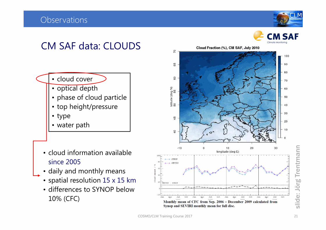
COSMO/CLM Training Course 2017 21
• cloud cover
• optical depth
• phase of cloud particle
• top height/pressure
• type
• water path
• cloud information available
since 2005
• daily and monthly means
• spatial resolution 15 x 15 km
• differences to SYNOP below
10% (CFC)
CM SAF data: CLOUDS
slid
e: Jö
rg T
ren
tma
nn

Observations
COSMO/CLM Training Course 2017 22
• surface solar irradiance
• Top-of-the atmosphere SW / LW
radiation
• surface radiation information
available since 1983
• hourly, daily and monthly means
• spatial resolution down to
0.03 deg
CM SAF data: RADIATION
slid
e: Jö
rgTr
en
tma
nn

Observations
COSMO/CLM Training Course 2017 23
• integrated water vapor
• water vapor / temperature
on 5 vertical levels
• precipitation (ocean only!)
• water vapor data available since 2004
• ocean only data (= precip, total water) available since 1987
• daily and monthly means, • spatial resolution 90 km• global mean difference (water vapor) to
radiosondes below 1 mm
CM SAF data: WATER VAPOR
slid
e: Jö
rgTr
en
tma
nn

Observations
COSMO/CLM Training Course 2017 24
Multi-model-mean (MMM)
E-OBS Reg. Data
GPCC
U-DEL
CRU
ERA-Int.HMRPRECGPCP
slid
e: A
nd
rea
s P
rein
The unknown truth

Observations
COSMO/CLM Training Course 2017 25
The unknown truth
Temperature and precipitation biasin the Alpine Region

Measures and Scores
Measures and Scores
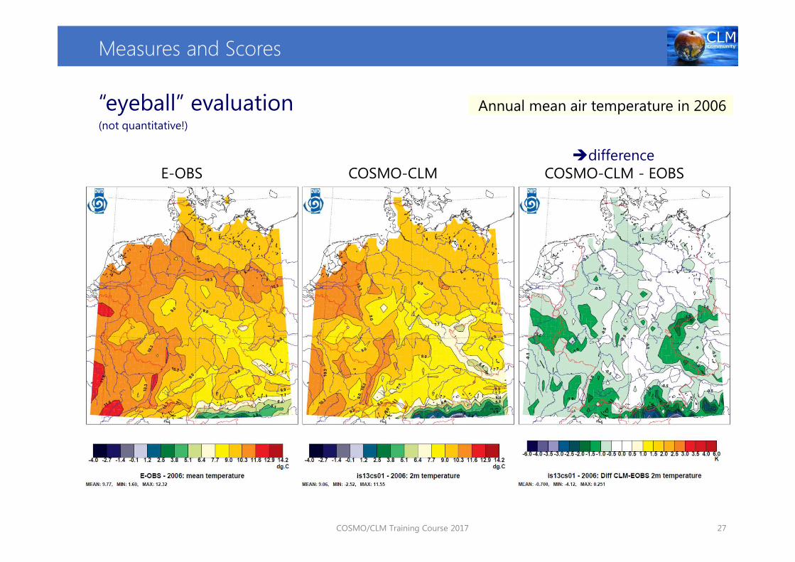
COSMO/CLM Training Course 2017 27
E-OBS COSMO-CLM - EOBS
Annual mean air temperature in 2006
COSMO-CLM
“eyeball” evaluation(not quantitative!)
�difference
Measures and Scores
COSMO/CLM Training Course 2017 28
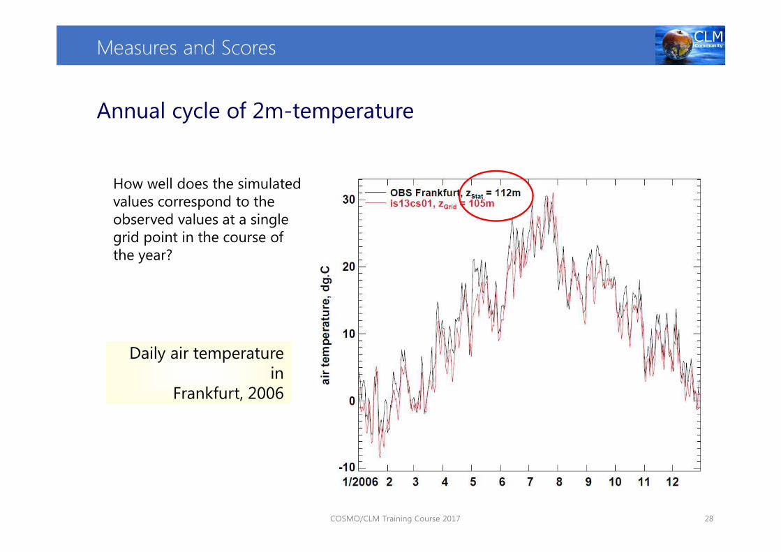
Annual cycle of 2m-temperature
Daily air temperature in
Frankfurt, 2006
How well does the simulated values correspond to the observed values at a single grid point in the course of the year?

Measures and Scores
COSMO/CLM Training Course 2017 29
Annual cycle of 2m-temperature
Monthly air temperature in Frankfurt, 2006
Measures and Scores
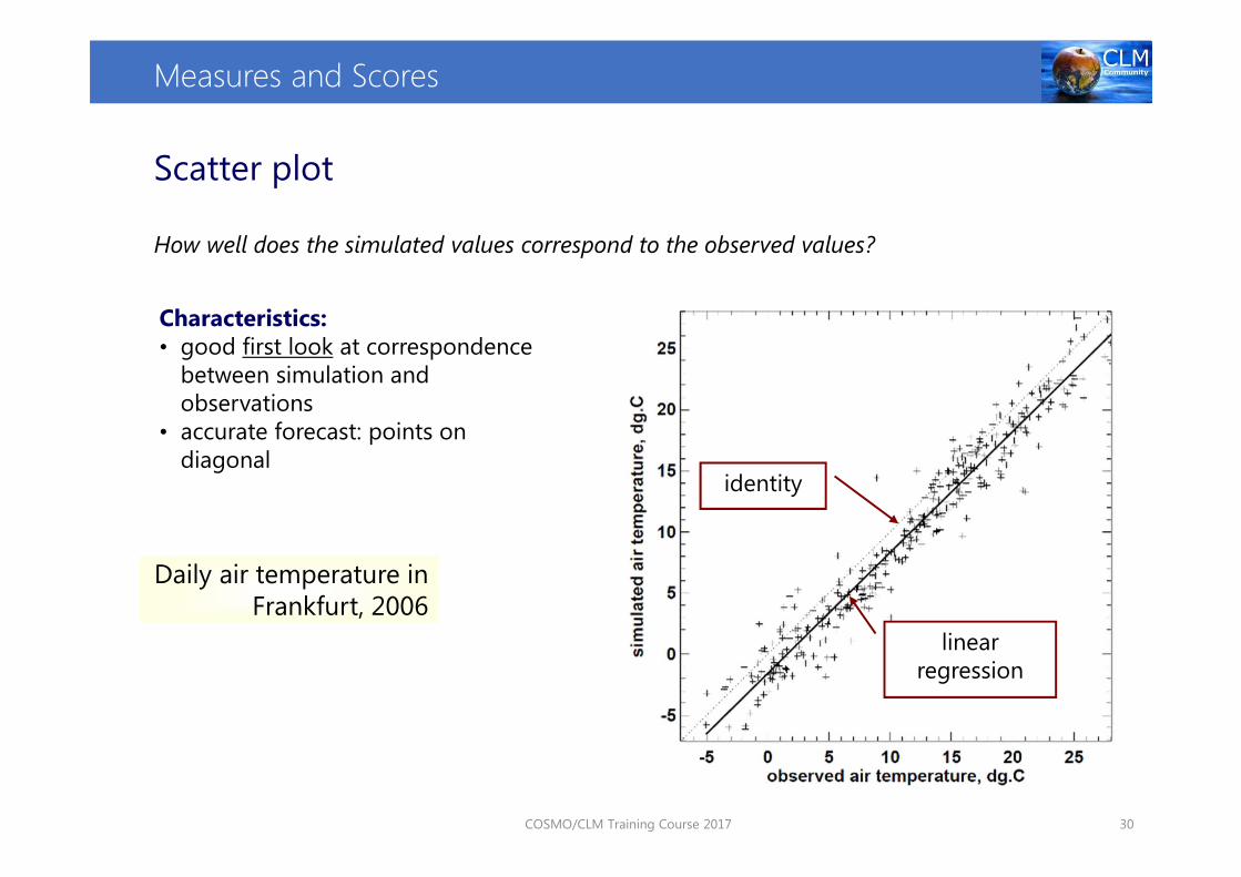
COSMO/CLM Training Course 2017 30
Scatter plot
How well does the simulated values correspond to the observed values?
Characteristics:• good first look at correspondence
between simulation and observations
• accurate forecast: points on diagonal
Daily air temperature inFrankfurt, 2006
linear regression
identity

Measures and Scores
COSMO/CLM Training Course 2017 31
Scatter plot – 2D-histogram
Characteristics:• good first look at correspondence
between simulation and observations
• better overview in case of many pairs
Daily air temperature inFrankfurt, 2006
How well does the simulated values correspond to the observed values?
Measures and Scores
COSMO/CLM Training Course 2017 32
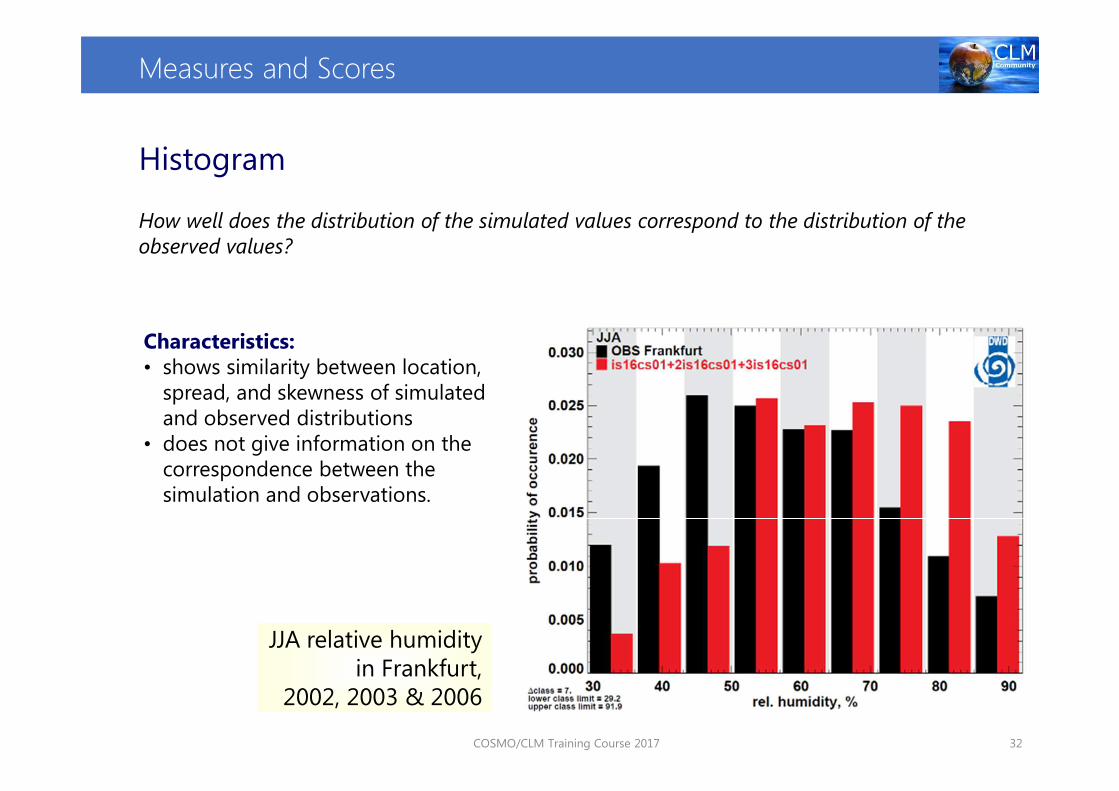
Histogram
How well does the distribution of the simulated values correspond to the distribution of the observed values?
JJA relative humidityin Frankfurt,
2002, 2003 & 2006
Characteristics:• shows similarity between location,
spread, and skewness of simulated and observed distributions
• does not give information on the correspondence between the simulation and observations.

Measures and Scores
COSMO/CLM Training Course 2017 33
Bias and mean absolute error
Bias (mean error)What is the average simulation error? Range: -∞ to ∞. Perfect score: 0. Characteristics:• simple, familiar• does not measure the magnitude of the errors• does not measure the correspondence between
simulation and observations• possibility of compensating errors
( )∑=
−=N
iii OS
Nerrormean
1
1
Mean absolute errorWhat is the average magnitude of the simulation errors? ∑
=
−=N
iii OS
NMAE
1
1
sou
rce
: C
AW
CR
Range: 0 to ∞. Perfect score: 0. Characteristics:• simple, familiar• does not indicate the direction of the deviations

Measures and Scores
COSMO/CLM Training Course 2017 34
Root mean squared error
sou
rce
: C
AW
CR
What is the average magnitude of the simulation errors?
( )∑=
−=N
iii OS
NRMSE
1
21Range: 0 to ∞. Perfect score: 0. Characteristics:• simple, familiar• measures "average" error, weighted according to the
square of the error• does not indicate the direction of the deviations• puts greater influence on large errors than smaller
errors

Measures and Scores
COSMO/CLM Training Course 2017 35
How well does the new test simulations perform as compared to an old reference simulation?
Range: -∞ to 1. Perfect score: 1.Characteristics:• based on ratio of root mean square differences
Brier Skill Score (BSS)
equal to
F is the „forcast“R is the reference „forecast“
Modification to a symmetric version with the range of -1 to 1
Measures and Scores
COSMO/CLM Training Course 2017 36
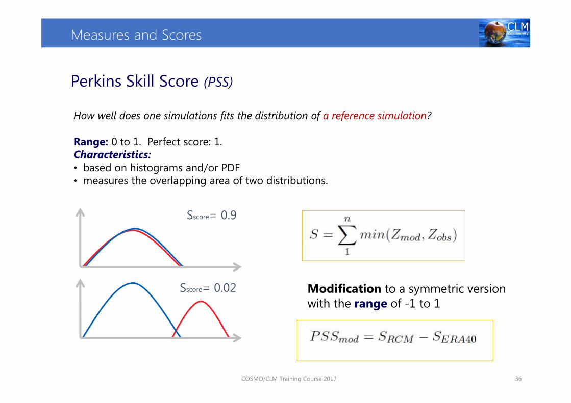
How well does one simulations fits the distribution of a reference simulation?
Range: 0 to 1. Perfect score: 1.Characteristics:• based on histograms and/or PDF• measures the overlapping area of two distributions.
Perkins Skill Score (PSS)
Sscore= 0.9
Sscore= 0.02 Modification to a symmetric versionwith the range of -1 to 1
Measures and Scores
COSMO/CLM Training Course 2017 37
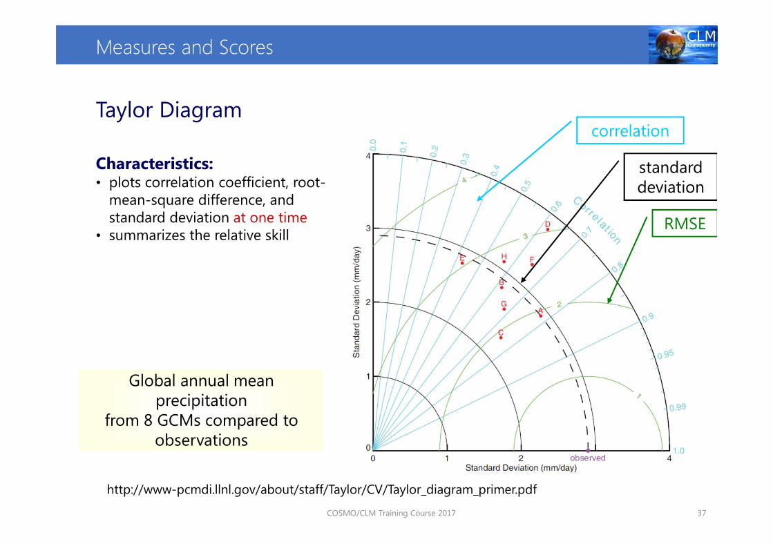
Taylor Diagram
http://www-pcmdi.llnl.gov/about/staff/Taylor/CV/Taylor_diagram_primer.pdf
Global annual mean precipitation
from 8 GCMs compared to observations
correlation
RMSE
standard deviation
Characteristics: • plots correlation coefficient, root-
mean-square difference, and standard deviation at one time
• summarizes the relative skill

Measures and Scores
COSMO/CLM Training Course 2017 38
Double Penalty
� threat of “double penalty” especially for variables, like precipitation, and measures with a higher weight on large deviations, like RMSE.
� solution: object oriented or position independent evaluation, e.g. SAL

Measures and Scores
COSMO/CLM Training Course 2017 39
SAL S tructure � size and shape
A mplitude � amount
L ocation � position
perfect score: S = A = L = 0
Wernli et al., 2008, MWR
Measures and Scores
COSMO/CLM Training Course 2017 40
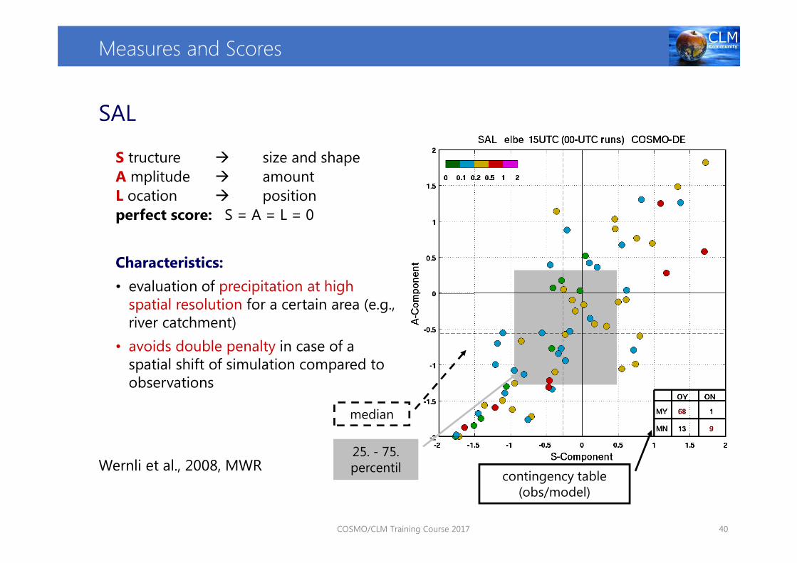
SAL
Characteristics:
• evaluation of precipitation at high spatial resolution for a certain area (e.g., river catchment)
• avoids double penalty in case of a spatial shift of simulation compared to observations
median
25. - 75. percentil
contingency table (obs/model)
S tructure � size and shape
A mplitude � amount
L ocation � position
perfect score: S = A = L = 0
Wernli et al., 2008, MWR

Measures and Scores
COSMO/CLM Training Course 2017 41
Significance
Does the hypothesis lead to changes by random chance?
In statistics, a result is called statistically significant if it is unlikely to have occurred by chance.
Does the sample represent the total population?
Confidence
Measures and Scores
COSMO/CLM Training Course 2017 42
Confidence Interval
� analytical solution in case of normally distributed variables
� otherwise frequently used: non-parametric bootstrapping*:estimating properties of an estimator (e.g., its variance) by measuring those properties when sampling from an approximating distribution
• standard choice for an approximating distribution:empirical distribution of the observed data.
• assumption for the set of observations:independent and identically distributed population
� constructing a number of resamples of the observed dataset (and of equal size to the observed dataset), each of which is obtained by random sampling with replacement from the original dataset.
*Efron and Tibshirani 1994
Measures and Scores
COSMO/CLM Training Course 2017 43
7,0
7,5
8,0
8,5
9,0
9,5
10,0
10,5
11,0
11,5
12,0
1950
1955
1960
1965
1970
1975
1980
1985
1990
1995
2000
2005
air
te
mp
era
ture
, °C
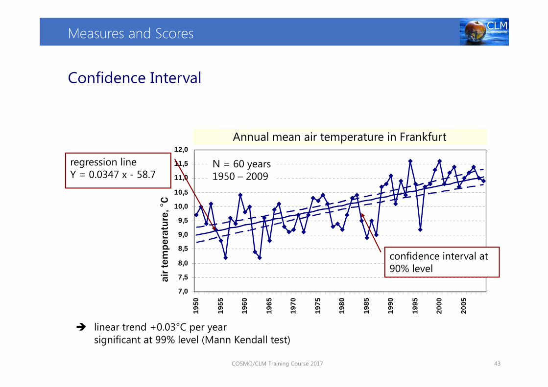
Annual mean air temperature in Frankfurt
N = 60 years1950 – 2009
regression lineY = 0.0347 x - 58.7
� linear trend +0.03°C per yearsignificant at 99% level (Mann Kendall test)
confidence interval at 90% level
Confidence Interval

Measures and Scores
COSMO/CLM Training Course 2017 44
Aim: to consider models and input uncertainty
�ensemble based on a single model:
� perturbations of the initial conditions –
to account for the non-linear dynamics
� perturbations of the boundary conditions –
to account for the ‘imperfect’ characterization of the non-
atmospheric components of the climate system and also
– in case of a regional model – for the uncertainty of the driving
global model
� perturbations of the model physics –
to account for the uncertainties inherent in the parameterizations
�multi model ensemble –
to account for the uncertainties inherent in the models themselves
Ensemble Simulations
Measures and Scores
COSMO/CLM Training Course 2017 45
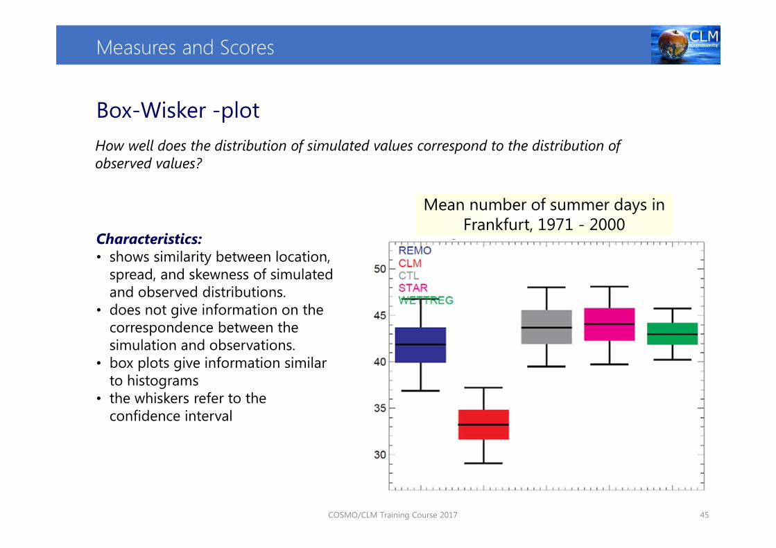
Box-Wisker -plot
Characteristics:• shows similarity between location,
spread, and skewness of simulated and observed distributions.
• does not give information on the correspondence between the simulation and observations.
• box plots give information similar to histograms
• the whiskers refer to the confidence interval
How well does the distribution of simulated values correspond to the distribution of observed values?
Mean number of summer days inFrankfurt, 1971 - 2000
Measures and Scores
COSMO/CLM Training Course 2017 46
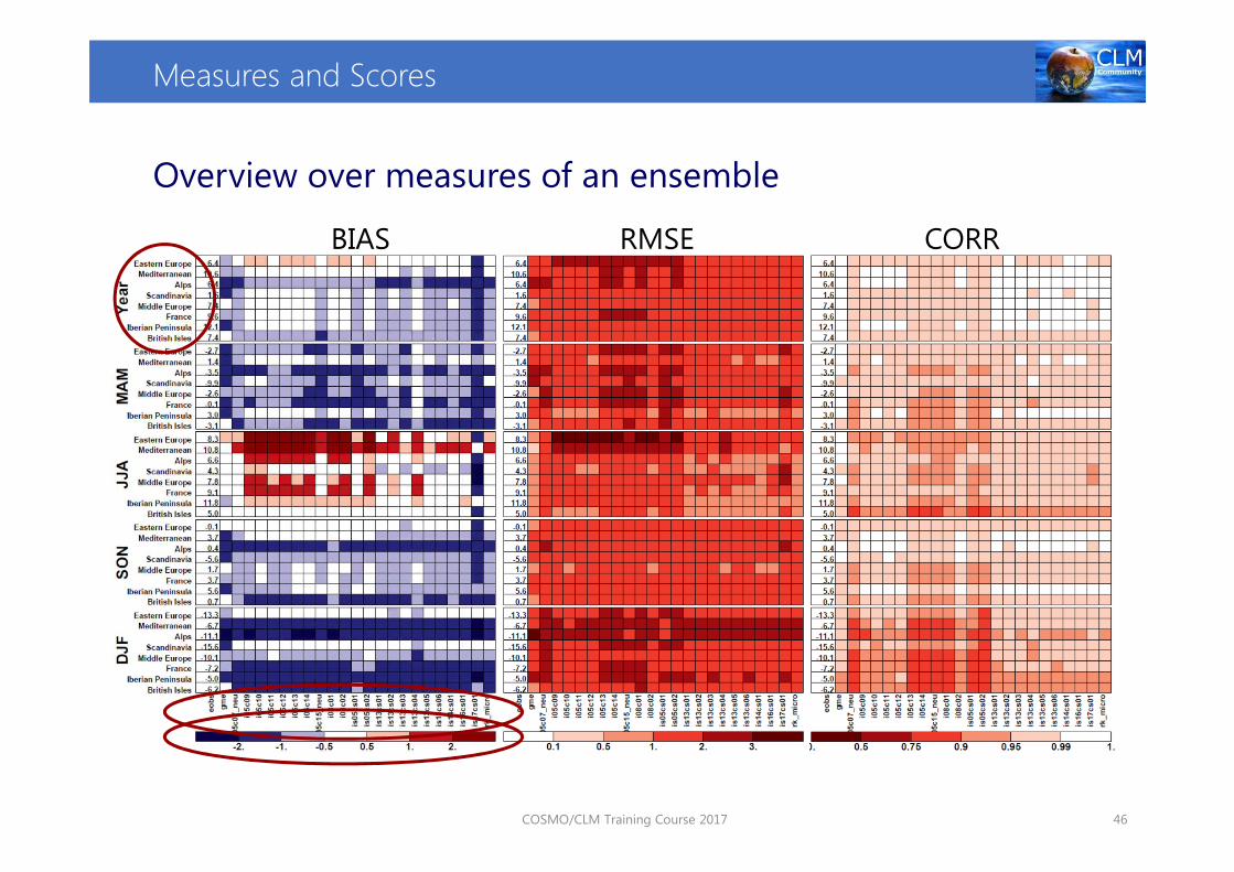
Overview over measures of an ensemble
BIAS CORRRMSE

ETOOL and ETOOL-VIS
ETOOL / ETOOL-VIS
COSMO/CLM Training Course 2017 48
What is ETOOL?
• csh-script which uses CDOs (Climate Data Operators*)
• it can be run at the command prompt or submitted to a batch-queue
• calculates simple statistics for different parameters (T_2M_AV, T_2M, TOT_PREC)
• easy to use and modify
• it can be found on the CLM-Community website> Model System > Utilities http://www.clm-community.eu/index.php?menuid=85
*https://code.zmaw.de/projects/cdo

COSMO/CLM Training Course 2017 49
What is ETOOL?
Following variables are evaluated:
• 2m air temperature: E-OBS
• 2m maximum temperature: E-OBS
• 2m minimum temperature: E-OBS
• 2m diurnal temperature range: E-OBS
• total precipitation: E-OBS
• mean sea level pressure: EOBS
• total cloud cover: CRU
ETOOL / ETOOL-VIS

Further development
• only Europe (E-OBS and CRU has been implemented so far. Also other data sets such as GPCC can be included to allow for global use.
• new standard regions would have to be implemented (e.g. for the CORDEX Africa-domain)
• it is possible to expand to other variables where a reference data set is available
• by the moment it will be extended to evaluate high resolutions simulations for the Alps and a Low Lang region Belgium/West-Germany to ETOOL-HD in WG-CRCS
• standardized plotting routine using NCL and R → E-TOOL-VIS
ETOOL / ETOOL-VIS

COSMO/CLM Training Course 2017 51
What is ETOOL-VIS?
ETOOL / ETOOL-VIS
For Europe or the 8 subregions
• area plot of clim. mean bias
• annual cycle of area mean bias
• Taylor diagr. of temporal variability
• Taylor diagr. of spatial variablity
• Brier Skill Score of temporal RMSE
• standardized plotting
• routine using NCL*
• based on E-TOOL outcome
• easy to modify
• Quick-Reference included
• CLM-Community website� Model System � Utilities
*http://www.ncl.ucar.edu/

COSMO/CLM Training Course 2017 52
What is ETOOL/ETOOL-VIS for?
make different simulations comparable
ETOOL / ETOOL-VIS

Example from WG-EVAL

COSMO/CLM Training Course 2017 54
Example from WG-EVAL
Simulation ID CCLM Version Namelist Configuration
CON031 4.8_clm19 Recommended standard configuration of old evaluation run
CON052 5.0_clm3 Standard configuration of old evaluation run transferred to new model version
CON069 5.0_clm6 Modified (recommended) configuration for new model version (see previous slide)
Definition of the new recommended model version is a main task of WG-EVAL
COPAT –COordinated Parameter Testing
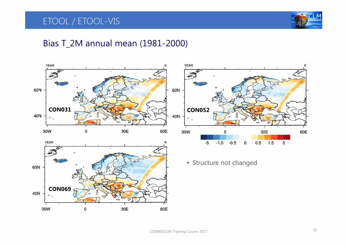
COSMO/CLM Training Course 2017 55
ETOOL / ETOOL-VIS
Bias T_2M annual mean (1981-2000)
• Structure not changed
CON069
CON052CON031

COSMO/CLM Training Course 2017 56
ETOOL / ETOOL-VIS
Bias TOTPREC annual mean (1981-2000)
• Structure not changed
CON069
CON052CON031
COSMO/CLM Training Course 2017 57
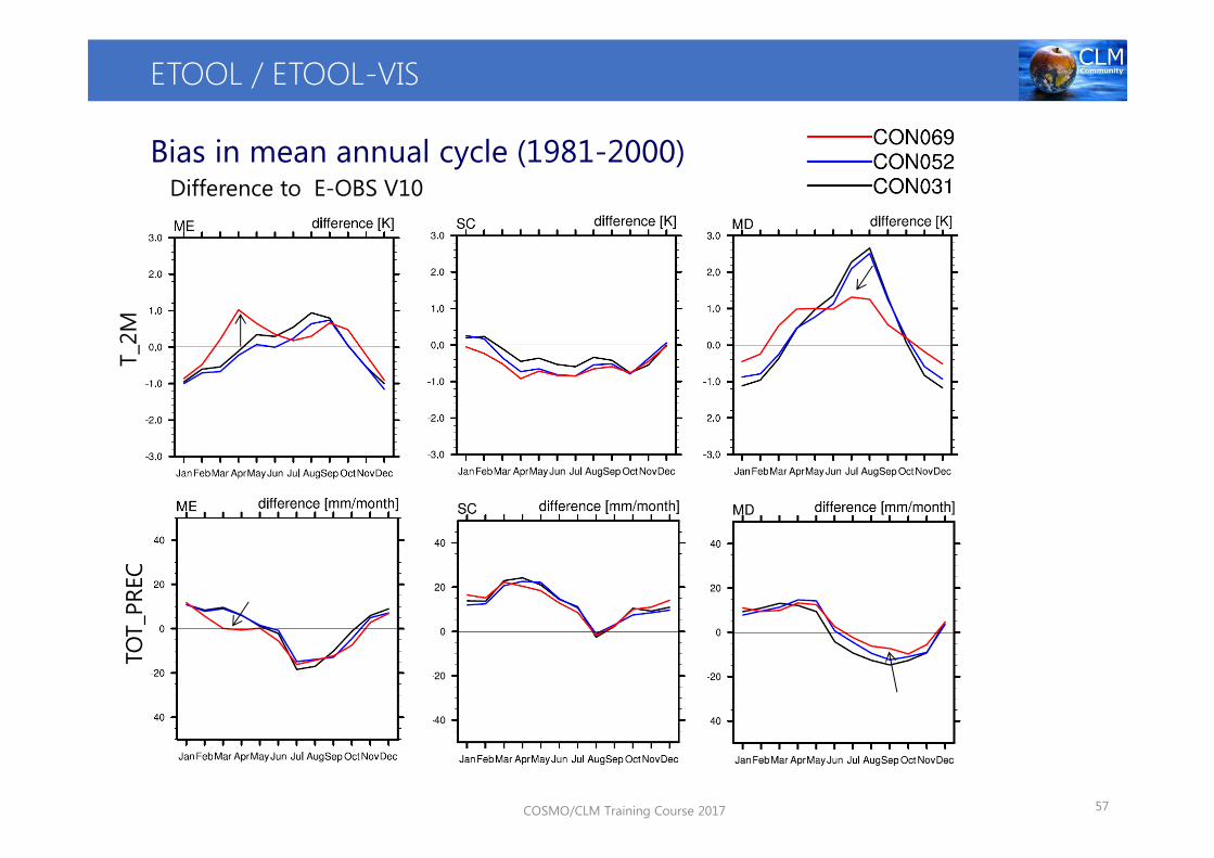
ETOOL / ETOOL-VIS
Bias in mean annual cycle (1981-2000)Difference to E-OBS V10
T_2
MTO
T_P
REC
COSMO/CLM Training Course 2017 58
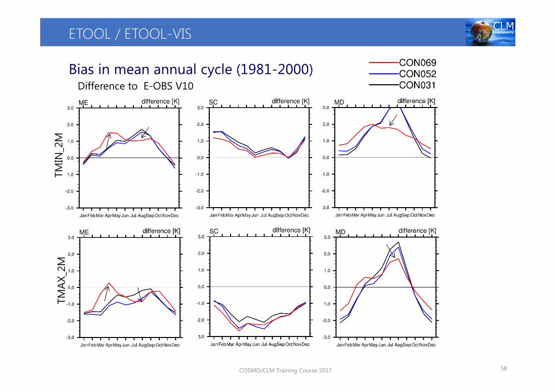
Difference to E-OBS V10
TM
IN_2
MTM
AX
_2M
ETOOL / ETOOL-VIS
Bias in mean annual cycle (1981-2000)

COSMO/CLM Training Course 2017 59
ETOOL / ETOOL-VIS
Taylor (interanual variation)T_2
MTO
T_P
REC
ME
ME
FR
FR
MD
IP
Difference to E-OBS V10

COSMO/CLM Training Course 2017 60
ETOOL / ETOOL-VIS
TM
IN_2
MTM
AX
_2M
ME
ME
FR
FR
IP
BI
Taylor (interanual variation)
Difference to E-OBS V10

COSMO/CLM Training Course 2017 61
ETOOL / ETOOL-VIS
Taylor (interannual variation)
Difference to E-OBS V10TO
T_P
REC
ME FR SC
TOT_P
REC
ME FR IP
tem
po
ral co
rrela
tio
nsp
ati
alco
rrela
tio
n

Observations
COSMO/CLM Training Course 2017 62
How well does the new test simulations perform as compared to an old reference simulation?
Range: -∞ to 1. Perfect score: 1.Characteristics:• based on ratio of root mean square differences
slid
e: K
lau
s K
eu
ler,
BTU
Brier Skill Score (BSS)
equal to
F is the „forcast“R is the reference „forecast“
Modification to a symmetric version with the range of -1 to 1

COSMO/CLM Training Course 2017 63
ETOOL / ETOOL-VIS
Brier Skill Score (BSS) - modified
Ref: CON031, Obs: EOBS-v10.0B
SS T
OT_P
REC
BSS T_2M

COSMO/CLM Training Course 2017 64
ETOOL / ETOOL-VIS
Brier Skill Score (BSS) - modified
Ref: CON031, Obs: EOBS-v10.0B
SS T
MIN
_2M
BSS TMAX_2M

COSMO/CLM Training Course 2017 65
ETOOL / ETOOL-VIS
Brier Skill Score (BSS) - modified
Run: CON069 vs Ref: CON031,
T_2M TOTPREC
TMIN_2M TMAX_2M

COSMO/CLM Training Course 2017 66
Example - Summary
CCLM5.0 with standard configuration of CCLM4.8 provides results comparable to old
standard evaluation
- deviations are smaller than between different resolutions
CCLM5.0 with new configuration (and tuning) changes climatological results
- partly improvements, but not for all regions and quantities
Precipitation
- annual cycle of area mean bias is nearly unchanged
- small improvements for MD, EA, AL
T_2M
- cold bias in winter reduced
- warm bias in summer partly reduced (IP,MD,EA,FR)
- new maximum warm bias in spring

Summary
TMAX_2M
- generally improved, except for SC
- negative bias is reduced
TMIN_2M
- effects are indifferent
- too high values are partly reduced but sometimes increased
PMSL
- systematically lower in all seasons and regions
- increased negative bias in summer up to -3 hPa
BSS for T_2M, TOT_PREC, TMIN, TMAX
- improved in all regions except SC
Influence of resolution cannot be neglected
- higher resolution mostly better but not always
- BSS are improved, annual cycle of precipitation not

Thank you!!!
And have a safe trip home!
See you at the CCLM Assembly in September in Graz