i

A NEW TUNING METHOD FOR TWO-DEGREE-OF-FREEDOM INTERNAL MODEL CONTROL UNDER PARAMETRIC UNCERTAINTY

JUWARI

Thesis submitted in fulfillment of the requirements for the award of the degree of

Doctor of Philosophy in Chemical Engineering

Faculty of Chemical and Natural Resources Engineering UNIVERSITI MALAYSIA PAHANG

MAY 2011

vii

ABSTRACT

The purpose of controller tuning is to determine the parameters of controller in order to ensure the time response of close-loop control system at the desired performance. Proportional Integral Derivative (PID) controller has been used in the industry since 1940’s for this purpose. However, the PID controller can not completely compensate for the complexity of industrial processes and desired high product quality due to interactions, nonlinearities, and time delay of the process variables. Internal model control (IMC) has been developed to overcome the deficiencies of the PID. Unfortunately, IMC yields very good performance for set point tracking, but gives sluggish response for disturbance rejection problem. The present study has developed a controller for disturbance rejection based on feedback / feedforward IMC structure. The controller is then called as feedback 2DOF-IMC. A new tuning method has been proposed for the controller. The proposed tuning method consists of three steps: Firstly, determine the worst case of the model uncertainty. Secondly, specify the parameter of set point controller using maximum peak (Mp) criteria. And thirdly, obtain the parameter of the disturbance rejection controller using gain margin (GM) criteria. The proposed method is called Mp-GM tuning method.

The effectiveness of the proposed feedback 2DOF-IMC and Mp-GM tuning method has evaluated and compared with standard 2DOF-IMC using IMCTUNE and Kaya 2DOF-IMC using Mp-GM tuning as bench mark. The evaluation and comparison are investigated through simulation and implementation on a number of first order plus dead time (FOPDT) and higher order processes. The FOPDT process tested include processes with controllability ratio in the range 0.7 to 2.5. The higher processes include second order with underdamped and third order with nonminimum phase processes. Although the two of higher order process are considered difficult processes, the proposed feedback 2DOF-IMC and Mp-GM tuning method were able to obtain the optimal controller even under process uncertainties. The proposed feedback 2DOF-IMC and the proposed Mp-GM tuning are also successfully implemented in real-time on a laboratory scale air heater pilot plant. The process model is divided into two regions. The time responses show that the proposed feedback 2DOF-IMC and the proposed Mp-GM tuning gave faster set point tracking and disturbance rejection responses than 1DOF-IMC and standard 2DOF-IMC in both regions.

viii

ABSTRAK

Tujuan dari talakan kontroler adalah untuk menentukan parameter pengawal iaitu memastikan waktu sambutan sistem kawalan gelung tertutup pada prestasi yang dikehendaki. Kawalan kamiran terbitan berkadaran (PID) telah digunakan dalam industri sejak tahun 1940 an untuk tujuan ini. Namun, pengawal PID tidak boleh sepenuhnya mengimbangi kekompleksan proses-proses industri dan kualiti produk yang dikehendaki. Ini karena tingginya interaksi antara proses, proses tak lelurus, dan masa tunda pembolehubah proses yang lama. Kawalan model dalam (IMC) telah dibangunkan untuk mengatasi kekurangan PID. Malangnya, IMC memberikan sambutan lamban untuk masalah penolakan gangguan. Penyelidikan ini telah membangunkan sebuah pengawal untuk penolakan gangguan berdasarkan struktur suap balik / suap depan IMC. Pengawal ini kemudian disebut sebagai suap balik 2DOF-IMC. Sebuah kaedah penalaan yang kuat dan sederhana telah dicadangkan untuk pengawal ini. Kaedah penalaan yang dicadangkan terdiri daripada tiga langkah: Pertama, menentukan kes terburuk dari ketidakpastian model.Kedua, menentukan parameter daripada pengawal titik set menggunakan kriteria puncak maksimum (Mp). Dan ketiga, menentukan parameter daripada pengawal penolakan gangguan menggunakan kriteria jidar gandaan (GM). Kaedah penalaan yang dicadangkan ini disebut Mp-GM.

Keberkesanan daripada suap balik 2DOF-IMC dan kaedah penalaan Mp-GM

yang dicadangkan dikaji dan dibandingkan dengan piawai 2DOF-IMC dengan penala IMCTUNE dan Kaya 2DOF-IMC dengan penala Mp-GM. Pengkajian dan perbandingan dilakukan melalui penyelakuan dan pelaksanaan di beberapa proses urutan pertama plus waktu mati (FOPDT) dan proses urutan yang lebih tinggi. Proses FOPDT yang diuji termasuk proses dengan nisbah kebolehkawalan daripada 0.7 sehingga 2.5. Proses urutan tinggi yang diuji adalah proses urutan kedua dengan tak teredam dan proses urutan ketiga dengan sistem fasa tak minimum. Walaupun dua proses urutan tinggi itu termasuk proses yang sukar, suap baik 2DOF-IMC dan kaedah penalaan Mp-GM yang dicadangkan boleh memberikan parameter pengawal yang optimum pada ketakpastian proses. suap baik 2DOF-IMC dan kaedah penalaan Mp-GM yang dicadangkan juga berjaya dilaksanakan secara masa nyata dengan skala makmal pada loji pandu pemanas udara. Model proses dibagi menjadi dua daerah. sambutan waktu menunjukkan bahawa maklum balas yang dicadangkan suap balik 2DOF-IMC dengan penala Mp-GM memberi sambutan penolakan yang lebih cepat dan mencapai set yang lebih cepat dibandingkan oleh 1DOF-IMC atau piawai 2DOF-IMC pada kedua-dua daerah.

ix

TABLE OF CONTENTS

Page

TITLE i

APPROVAL DOCUMENT ii

SUPERVISOR’S DECLARATION iii

STUDENT’S DECLARATION iv

DEDICATIONS v

ACKNOWLEDGEMENTS vi

ABSTRACT vii

ABSTRAK viii

TABLE OF CONTENTS ix

LIST OF TABLES xii

LIST OF FIGURES xiii

LIST OF SYMBOLS xvi

LIST OF ABBREVIATIONS xviii

CHAPTER 1 INTRODUCTION

   

1.1 Introduction 1

1.2 Internal model control (IMC) 2

1.3 Two-Degree-of- Freedom Internal Model Control (2DOF-IMC) 2

1.3 Problem Statements 3

1.4 Objectives and Scope of the Research 4

1.5 Methodology of the Research 5

1.6 Contributions of the Research 6

1.7 Structure of the Thesis 7

 

CHAPTER 2 INTERNAL MODEL CONTROL

   

2.1 Introduction 9

2.2 Structure of Standard Internal Model Control 10

2.2.1 Principle of IMC controller 10 2.2.2 Advantages of 1DOF-IMC 13

x

2.2.3 Limitations of 1DOF-IMC 14 2.2.4 2DOF-IMC 16 2.2.5 1DOF and 2DOF IMC for PID controller design 16

2.3 Chemical Process Uncertainty 18

2.4 Tuning of IMC Under Model Uncertainty 21

2.4.1 Tuning of 1DOF-IMC 21 2.4.2 Tuning of 2DOF-IMC 30

2.5 Summary 35

   

CHAPTER 3 NEW Mp-GM TUNING METHOD FOR 2DOF-IMC

   

3.1 Introduction 37

3.2 Maximum Peak (Mp) 38

3.3 Gain Margin 41

3.4 Mp-GM Tuning Method of 2DOF-IMC 43

3.4.1 Structure of feedback/feedforward 2DOF-IMC 43 3.4.2 Procedure Mp-GM tuning method for 2DOF-IMC 46 3.4.3 Comparison of parameter and time response of proposed

feedback and standard 2DOF-IMC 48

3.4.4 Effects of Mp value to output responses. 54 3.4.5 Effect of ratio λ2 to λ1 56 3.4.6 Effect of GM to output response 59 3.4.7 Effect of simplification model (Gpm) and controller form 63 3.4.7.1 Second order with underdamped process 63 3.4.7.2 Third order with non minimum phase process 68

3.5 Summary 70

   

CHAPTER 4 EXPERIMENTAL IMPLEMENTATION OF

PROPOSED Mp-GM TUNING METHOD  

   

4.1 Introduction 72

4.2 Plant Descriptions 72

4.3 Experimental Setup 74

4.4 Model Identification and Controller Tuning 78

4.4.1 Model identification using step response model 78 4.4.2 The controller tuning and time responses of AFPT pilot

plant 82

xi

4.5 Summary 85

   

CHAPTER 5 CONCLUSIONS AND RECOMMENDATIONS

   

5.1 Conclusions 87

5.2 Recommendations for the Future Works 89

 

REFERENCES 90

APPENDICES

A List of Publications 95

B Matlab Code of Proposed Mp-GM Tuning for 2DOF-IMC 96

C Tuning Procedure of IMCTUNE 99

D Butterworth Filter Code Using Matlab S-Function 101

     

xii

LIST OF TABLE

Table No. Title Page

3.1 Parameters of 2DOF-IMC, FOPDT with θ/τ > 1 50

3.2 The IAE value of FOPDT process with θ/τ > 1 54

3.3 Controller parameters and its percentage overshoot 55

3.4 The value of λ2 and α for the corresponding λ2/λ1 56

3.5 Effect of λ2/λ1 to output response 57

3.6  IAE values at difference GM specification 60

4.1 The FOPDT step response models of the plant 81

4.2 Two regions of process model of AFPT pilot plant. 82

4.3 The three controller parameters for both of regions. 83

xiii

LIST OF FIGURES

Figure No. Title Page

1.1 Structure of standard IMC controller 2

1.2 Structure of standard 2DOF-IMC 3

2.1 Simplified IMC controller to classical feedback control 10

2.2 Additive (la) dan multiplicative (lm) uncertainty 19

2.3 The uncertainty region π(ω)  evaluated at a ω value. The smallest circle containing  π(ω)  could be used as a norm-bounded approximation to the actual uncertainty. (Laughlin et al., 1986)  

23

2.4 Uncertainty region  π(ω)  for 30 frequencies range 0.001-1. The nominal model passes through the center of each region. (Laughlin et al., 1986)  

23

2.5 Uncertainty region  π(ω)  Gc1(j ω)  on Nyquist plane. Robust stability requires that none of the regions contain the critical  (‐1,j0). (Laughlin et al., 1986)  

24

2.6 Iterative learning IMC controller by Liu et al. (2010) 29

2.7 2DOF-IMC proposed by Kaya (2004) 33

2.8 2DOF controller used by Shreesha and Gudi (2003) 34

3.1 General structure of a feedback control system. 39

3.2 Resonant peak (Mp) Vs frequency. (Levine, 1995) 39

3.3 Correlations between Mp, OS and ζ . (Nagrath and Gopal, 2006)  

41

3.4 Gain and phase gain margins on Nyquist plot. 42

3.5 Classic feedback/feedforward control structure. 43

3.6 Feedback/feedforward IMC controller. 44

3.7 2DOF IMC from feedback/feedforward structure. 46

3.8 Tuning output of the proposed feedback 2DOF-IMC controller. 49

xiv

Figure No. Title Page

3.9 The magnitude of |T (j ω)| vs frequency (ω).  51

3.10 Interpretation gain margin of FOPDT process on Nyquist plot of proposed feedback 2DOF-IMC

51

3.11 Interpretation gain margin of FOPDT process on Nyquist plot of Kaya 2DOF-IMC  

52

3.12 Time response of the feedback 2DOF-IMC and standard 2DOF-IMC, FOPDT with θ/τ > 1  

53

3.13 The output response for no-error in the model are imposed, FOPDT with  θ/τ > 1  

54

3.14 The output response for slowest case, FOPDT with θ/τ > 1 54

3.15 Effects of Mp value to output response of FOPDT θ/τ > 1 55

3.16 Controller parameters of the standard 2DOF-IMC with IMCTUNE, FOPDT θ/τ < 1

57

3.17 The worst case responses for the case FOPDT with θ/τ < 1 58

3.18 The responses of the case FOPDT with θ/τ  <  1 with no error in the model.

58

3.19 The worst case responses for the case FOPDT with θ/τ < 1 59

3.20 The worst case responses of FOPDT with θ/τ ≅ 1 61

3.21 The responses of FOPDT with θ/τ ≅ 1 with no error in the model

61

3.22 The output responses of FOPDT with θ/τ ≅ 1 for the slowest case

62

3.23 Nyquist plot of FOPDT with θ/τ ≅ 1, GM = 1.7 62

3.24 Nyquist plot of FOPDT with θ/τ ≅ 1, GM = 3.1 63

3.25 FOPDT approximation of second order underdamped process 65

3.26 Nyquist plot of Mp GM tuning for underdamp SOPDT system with controller transfer functions are FOPDT form

66

xv

Figure No. Title Page

3.27 Nyquist plot of Mp GM tuning for underdamp SOPDT system with Gc1 is FOPDT form and Gc2 is SOPDT form

66

3.28 Time response of second order with underdamped process using two form controller strategies

67

3.29 GM criteria of third order with nonminimum phase process on the Niquist plot

69

3.30 Time response of controller design for non minimum phase with high order process

70

4.1 Air heater system. 73

4.2 Installation of heating element in asbestos cement board. 73

4.3 Installation of heating element and asbestos cement in galvanized pipe.

73

4.4 The field signal connected to DCS. 74

4.5 Human interface of AFPT pilot plant of deltaV workstation. 75

4.6 I/O connector. 75

4.7 (a) Human interface in matlab simulink program, (b) Analog ouput Data acquisition toolbox in simulink, and (c) Analog input data acquisition toolbox.

77

4.8 Step responses of the plant from 30% to 40%, 40% to 30%, and 30% to 20 %.

79

4.9 Step responses of the plant from 5% to 30% with increment 5% 79

4.10 Step responses of the plant from 20% to 10% and 10% to 20% 80

4.11 Step responses of the plant from 15% to 10% to 5% 80

4.12 Identification of FOPDT model 81

4.13 The responses of the three controllers system on region 1 84

4.14 The time responses of the three controllers system on region 2 85

xvi

LIST OF SYMBOLS

d Disturbance input

e Error between measurement and model

E Error between e and set point

Gc Transfer function of controller

Gc1 Transfer function of set point controller

Gc2 Transfer function of disturbance rejection controller

Gcf Transfer function feedforward controller

Gd Transfer function of disturbance

Gp Transfer function of process

Gpm Treansfer function of model

k Gain of process

Kc Proportional gain

la Additive uncertainty

lm Multiplicative uncertainty

N Order of Butterworth filter

r Order of controller

s Laplace domain

S Sensitivity function

T Complementary sensitivity function

w Weighting function

y Measurement

ysp Set point

xvii

∆ Any stable transfer function which at each frequency is less than or equal to 1 magnitude

α Lead constant of Gc2 controller

β Lead constant of adding transfer function

λ Filter time constant

θ Time delay

τ Time constant of process

τD  Derivative time constant

τI  Integral time constant

ω Frequency

xviii

LIST OF ABBREVIATIONS

1DOF-IMC One- degree-of-freedom Internal Model Control (generally as IMC)

2DOF-IMC Two-degree-of-freedom Internal Model Control

AFPT Air Flow Pressure Temperature Control system Pilot Plant

FOPDT First Order plus Dead Time

GM Gain Margin

IAE Integral Absolute Error

IMC Internal Model Control

MIMO Multi Input Multi Output

Mp Maximum peak (or resonant peak)

MPC Model Predictive control

PID Proportional Integral Derivative

SISO Single Input Single Output

SOPDT Second Order Plus Dead Time

SP Smith Predictor controller

1

CHAPTER 1

INTRODUCTION

1.1 INTRODUCTION

A chemical industry generally consists of many unit operations, which must be

operated on a specific operating condition such as: temperature, pressure, and flow. This

operating condition(s) is maintained for the purpose of safety and product quality.

Proportional Integral Derivative (PID) controller has been used in the industry since

1940’s for this purpose because the PID controller uses a simple algorithm (Willis,

1999). Various designs and tuning strategies were developed for the PID controller so

that the controller can be used for various process characteristics. However, the PID

controller can not completely compensate for the complexity of industrial processes and

desired high product quality due to interactions, nonlinearities, and time delay of the

process variables (Anandanatarajan et al., 2006; Normey-Rico and Camacho, 2007).

The rapid development of computer technologies has encouraged the development of

various types of controllers to overcome the deficiencies of the PID. These controllers

include Artificial Neural Network (ANN) controller (Hussain and Ho, 2004; Mohanty,

2009), Fuzzy Logic controller (Galluzzo and Cosenza, 2009; Sarma and Rengaswamy,

2000) and Model Predictive Control (MPC) (Bezzo et al., 2005; Nikandrov and Swartz,

2009; Qin and Badgwell, 2003).

Internal Model Control (IMC) is a class of model based control proposed by

Garcia and Morari (1982). The structure of IMC controller is shown in Figure (1.1).

IMC uses a model explicitly and it is internally stable. This implies that if a plant is

stable, the stability of the process response can be guaranteed by using a controller with

stable model.

2

1.2 INTERNAL MODEL CONTROL (IMC)

The principle of IMC structure can be explained from (Figure 1.1); Gpm is

process model. Difference between model response and actual measurement (e) is used

as input signal to IMC controller (Gc1). In general, e ≠ 0, due to the modeling error and

unknown disturbances (d Gd) that are not accounted in the process model (Seborg et al.,

2004). Unfortunately, IMC controller provides a very slow response to the case of

disturbance rejection. Therefore, several researchers have attempted to overcome this

weakness by developing two-degree-of freedom-IMC (2DOF-IMC) (Morari and

Zafiriou, 1989). Figure 1.2 shows the standard structure of 2DOF-IMC controller.

Figure 1.1 Structure of standard IMC controller

Where e is error between measurement and model, E is error between set point and e,

Gp is transfer function of the process, Gpm is transfer function of the model and Gc1 is

transfer function of the controller, ysp is set point value, y is controlled variable, d is

disturbance input, and Gd is disturbance transfer function.

1.3 TWO-DEGREE-OF- FREEDOM INTERNAL MODEL CONTROL

(2DOF-IMC)

Figure 1.2 shows the controller for set point (Gc1) and the controller for

disturbance rejection (Gc2) in a 2DOF-IMC structure. The set point controller is in an

open loop form and the disturbance rejection controller is in a feedback structure. The

parameter of set point controller is designed as 1DOF-IMC controller, while the

Gc1 Gp y

Gpm

ysp

IMC Controller

E

e

- +

+ -

++

Gd d

3

disturbance rejection controller is designed such that the disturbance can be rejected as

soon as possible.

Figure 1.2 Structure of standard 2DOF-IMC

These tuning parameters can be easily obtained in the case of no error in the

model. However, the setting of parameter becomes a complicated matter if there is an

uncertainty model. On the other hand, the models developed will always contain

inaccuracies or contain uncertainty.

The model uncertainty comes from several sources as follows (Laughlin et al,

1986);

(i) The variation of real parameters affecting plant operation.

(ii) The inherent non-linearity of the processes.

(iii) The experimental identification of the process.

(iv) The mathematical model development.

1.4 PROBLEM STATEMENTS

As mentioned in the previous section the tuning parameters in the case of model

uncertainty is difficult to obtain. Many researchers have tried at different ways in tuning

of 1DOF-IMC based on model uncertainty (Brosilow and Joseph, 2001; Laughlin et al.,

1986; Liu et al., 1998; Morari and Zafiriou, 1989). Several works concentrating on the

2DOF-IMC tuning based on model uncertainty has done by Brosilow and Joseph (2001),

Gd

Gc1 Gp y

Gpm

ysp E

e

- +

+ -

++

d

Gc2

4

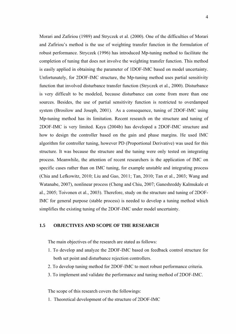
Morari and Zafiriou (1989) and Stryczek et al. (2000). One of the difficulties of Morari

and Zafiriou’s method is the use of weighting transfer function in the formulation of

robust performance. Stryczek (1996) has introduced Mp-tuning method to facilitate the

completion of tuning that does not involve the weighting transfer function. This method

is easily applied in obtaining the parameter of 1DOF-IMC based on model uncertainty.

Unfortunately, for 2DOF-IMC structure, the Mp-tuning method uses partial sensitivity

function that involved disturbance transfer function (Stryczek et al., 2000). Disturbance

is very difficult to be modeled, because disturbance can come from more than one

sources. Besides, the use of partial sensitivity function is restricted to overdamped

system (Brosilow and Joseph, 2001). As a consequence, tuning of 2DOF-IMC using

Mp-tuning method has its limitation. Recent research on the structure and tuning of

2DOF-IMC is very limited. Kaya (2004b) has developed a 2DOF-IMC structure and

how to design the controller based on the gain and phase margins. He used IMC

algorithm for controller tuning, however PD (Proportional Derivative) was used for this

structure. It was because the structure and the tuning were only tested on integrating

process. Meanwhile, the attention of recent researchers is the application of IMC on

specific cases rather than on IMC tuning, for example unstable and integrating process

(Chia and Lefkowitz, 2010; Liu and Gao, 2011; Tan, 2010; Tan et al., 2003; Wang and

Watanabe, 2007), nonlinear process (Cheng and Chiu, 2007; Ganeshreddy Kalmukale et

al., 2005; Toivonen et al., 2003). Therefore, study on the structure and tuning of 2DOF-

IMC for general purpose (stable process) is needed to develop a tuning method which

simplifies the existing tuning of the 2DOF-IMC under model uncertainty.

1.5 OBJECTIVES AND SCOPE OF THE RESEARCH

The main objectives of the research are stated as follows:

1. To develop and analyze the 2DOF-IMC based on feedback control structure for

both set point and disturbance rejection controllers.

2. To develop tuning method for 2DOF-IMC to meet robust performance criteria.

3. To implement and validate the performance and tuning method of 2DOF-IMC.

The scope of this research covers the followings:

1. Theoretical development of the structure of 2DOF-IMC

5

2. Theoretical review of the maximum peak and gain margin for 2DOF-IMC tuning.

3. Determine the optimal constants that involved in the tuning of 2DOF-IMC.

4. Simulation of several process characteristics that employ the structure and the

tuning method of 2DOF-IMC.

5. Application of the proposed method to experimental study in AFPT (air flow

pressure and temperature control system) pilot plant made by Syntec Sdn Bhd.

The plant is installed in laboratory of Chemical and Natural Recourses

Engineering University Malaysia Pahang. The experimental process is modeled

as FOPDT.

1.6 METHODOLOGY OF THE RESEARCH

The objectives of the research can be realized by creating a new structure of

2DOF-IMC into feedback control structure. By using feedback control structure, the

principle of robust performance that is usually used in conventional control such as

maximum peak (Mp) or resonant peak and gain margin (GM) can be applied.

Resonant peak (Mp) and its relationship between time responses of IMC

structure has been studied by (Brosilow and Joseph, 2001) using Mp-Tuning (maximum

peak) method. The maximum peak is the maximum of magnitude of frequency response

of complementary sensitivity function set as 1.05. This value corresponds to about 10%

overshoot of time response. With this method the parameters of the set point controller

on the model uncertainty can easily be determined.

The difficulties in tuning of disturbance rejection controller can be solved by the

principle of Gain Margin. Gain margin is a criterion that often used to measure the

stability of a control system (Kuo, 1995). In the Nyquist plot, gain margin is the

frequency response of open loop transfer function on the real and imaginary axis

(Seborg et al., 2004). Open loop transfer function of proposed feedback 2DOF-IMC can

be derived easily. The disturbance rejection controller parameters can be determined

using this method after the set point controller parameter is calculated.

6

There are three specifications in the Mp-GM tuning that needs to be specified

i.e; Mp, λ2/λ1 and GM. The best Mp value is determined where the overshot of the

worst case should not exceed than 10%. The value of the λ2/λ1 and GM is determined

from the closed loop response, where the corresponding minimum average of ISE

(Integral Square Error) value in the worst case, nominal case and slowest case will be

selected as tuning parameter. The Specifications above are selected with FOPDT

simulation process with θ/τ = 1, θ/τ > 1 and θ/τ <1.

The proposed feedback 2DOF-IMC structure and proposed Mp-GM tuning

method are evaluated both in simulation and experimental. For simulation, this work

studies;

(i) FOPDT (first order plus dead time) transfer function. It is because; typically

chemical process can be approximated by FOPDT form. Three

characteristics of FOPDT are analyzed i.e FOPDT with θ/τ (ratio between

time delay and time constant) equal to 1, less than 1 and more than 1.

(ii) Higher order process i.e SOPDT (second order plus dead time) with

underdamped and third order with non-minimum phase system.

The proposed structure and tuning method is also evaluated in nonlinear process of

AFPT (air flow pressure temperature) control system pilot plant. The detail of AFPT

pilot plant is presented in experimental study (Chapter 4).

Closed-loop response of the proposed feedback 2DOF-IMC with Mp-GM tuning

is compared with the standard 2DOF-IMC with IMCTUNE and Kaya 2DOF-IMC with

Mp-GM tuning. However, when IMCTUNE could not calculate the controller

parameters then standard 1DOF-IMC with IMCTUNE is performed. If standard 1DOF-

IMC with IMCTUNE still could not calculate the parameters then 1DOF-IMC with Mp-

GM is applied.

7

1.7 CONTRIBUTIONS OF THE RESEARCH

The main research contributions from this study are as follows:

1. New 2DOF-IMC structure based on feedback/feedforward control structure was

proposed. It is designed and simulated for open loop stable process which

commonly representing the chemical process system.

2. New robust and simple method to tune parameters of 2DOF-IMC was employed

using Mp-GM (Maximum peak and Gain Margin) criteria.

3. An air heater control system has been developed in laboratory for experimental

study in order to validate the above finding.

1.8 STRUCTURE OF THE THESIS

Chapter 2 reviews the related literatures about the weaknesses, advantages,

design and tuning of 1DOF-IMC controller structure. The design and tuning of 2DOF-

IMC under model uncertainty are reviewed and the chemical process uncertainty is

described.

Chapter 3 discusses the proposed Mp-GM tuning for 2DOF-IMC. The proposed

tuning method is derived from proposed design of 2DOF-IMC based on

feedback/feedforward structure control system (feedback 2DOF-IMC). The method can

then be implemented to a standard 2DOF-IMC structure. The results are compared with

some existing tuning method of 2DOF-IMC. The Mp-GM tuning is applied to several

FOPDT process from small to long time delay. There are three specifications that affect

to closed loop time response using Mp-GM tuning i.e; maximum peak (Mp), ratio filter

time constant of set point and disturbance rejection controller (λ1/λ2), and gain margin’s

values. The specifications are determined by simulating of FOPDT model. The effects

of simplification model are described with examples by using simulation of difficult

higher order process such as underdamped and nonminimum phase system. The closed

loop responses of proposed structure 2DOF-IMC and Mp-GM method are compared to

standard 2DOF-IMC with IMCTUNE and Kaya 2DOF-IMC with Mp-GM.

8

Chapter 4 describes the implementation of feedback 2DOF-IMC and Mp-GM

tuning method to the air heater system in AFPT pilot plant. The AFPT pilot plant is a

nonlinear plant particularly in the low to medium temperature range. It has nearly linear

model at high temperature range. Therefore, the effects of nominal model selection in

different range of operating conditions are presented in this chapter.

Finally, chapter 5 concludes the research study. Summarizes the results obtained

from previous chapters. The recommendations for future work are outlined. The

recommendations are given based on assessment of the significant findings, limitations,

conclusions obtained and difficulties encountered in this study.

9

CHAPTER 2

LITERATURE REVIEW

2.1 INTRODUCTION

The IMC was developed by Morari and coworkers (Garcia and Morari, 1982;

Morari and Zafiriou, 1989; Rivera et al., 1986). Internal Model Control (IMC) is a type

of model based control that has applied in the process industry (Brosilow and Joseph,

2001). IMC uses model explicitly in controller algorithm. This controller is actually a

generation of Smith predictor (SP) controller which was designed for a process with

long time delay (Smith O, 1959). The standard PID controller can not handle them

optimally because (Kaya, 2003; Normey-Rico and Camacho, 2007; Romagnoli and

Palazoglu, 2005);

- The disturbances are not detected immediately (detected until certain time

with delay).

- The control actions based on the delay is not in accordance with the

purposes of information.

- The control action took some time to determine its effects on the process.

Smith (1959) proposed delay compensator that aims to eliminate the delay

element of the feedback loop. This was done by including delay model in the controller

algorithm (Romagnoli and Palazoglu, 2005). SP controller has some weaknesses. If the

primary controller is not properly tuned, may be unstable when a small mismatch in the

dead time is considered (Palmor, 1980) and the disturbance rejection response can not

be faster than the open loop (Normey-Rico and Camacho, 2007). These weaknesses

could be overcome by IMC. SP can be considered as part of IMC. Modified version of

SP controller such as Filtered-SP (FSP), Filtered Predictive Proportional Integral (FPPI),

10

Two Degree of Freedom-Dead Time compensator (2DOF-DTC) and Dead Time

Observer disturbance compensator (DO-DTC) can be represented by the 2DOF- IMC

(Normey-Rico and Camacho, 2007). The advantages and weaknesses of IMC are further

discussed in section 2.2.

2.2 STRUCTURE OF STANDARD INTERNAL MODEL CONTROL

2.2.1 Principle of IMC controller

The structure of a standard IMC controller illustrated in Figure 1.1 can be

simplified into classical control feedback (Figure 2.1) (Chia and Lefkowitz, 2010).

Figure 2.1 Simplified IMC controller to classical feedback control

Gc Gp y ysp + -

++

Gd d

Gc1 Gp y

Gpm

ysp

IMC Controller

+

+

+ -

++

Gd d

Classical controller

11

From Figure 2.1 the classical controller (Gc) can be derived as follow

mGpGc

GcGc.1 1

1−

= (2.1)

It shows that the classical controller can be derived from IMC controller structure, or

the IMC controller can be analogous to the classical controller Gc. However, it is very

easy to design Gc1 than to design Gc. this is because some properties following IMC

structure (Economou and Morari, 1986):

Property 1: Assuming that the process model is the same as the plant then the closed

loop stability can be guaranteed if the plant and the controller is stable.

Property 2: Assuming that the controller Gc1 = 1 / Gpm generate a stable IMC structure,

then a perfect set point controller can be achieved.

Property 3: For all Gc1 with Gc1 (0) = 1 / Gpm (0) produces a stable IMC structure, then

an offset free control can be achieved.

The first property can be seen from equation 2.1 in which the stability of the

closed loop response is only affected by the stability of the plant and controller. While

the second character can be derived as follows. For the SISO system, the IMC controller

can be derived from Eq. (2.2) to (2.4) (Morari and Zafiriou, 1989).

Eeysp =− (2.2)

EGcGpye m 1−= (2.3)

Then,

EGcGpEyy msp 1−=− (2.4)

E* EGcGpm )1( 1−= (2.5)

Where e is error between measurement and model, E is error between set point and e

(see Figure 1.1), Gp is transfer function of the process, Gpm is transfer function of the

model and Gc1 is transfer function of the controller. The other abbreviations that are

12

used in Figure 2.1 and in the next figures are; Gd is transfer function of disturbance, d

input of the disturbance, ysp is setpoint input and y is a process variable (measurement /

controlled variable).

In the nominal case Gp = Gpm. Gc1 is designed to yield minimum value of E*;

212 )1(min*min11

EGcGpE mGcGc

−= (2.6)

In order to get minimal value of E*,

Gc1 = 1/Gpm. (2.7)

Eq. (2.6) states that optimal controller can be achieved if Gc1 = 1/Gpm (Eq.2.7) or the

error will be zero. It means that the process variable is always the same with set point.

However, Gc = 1/Gpm does not apply in some cases such as processes which has right

half plane zero and time delay. Fortunately, It can be done by following two steps as

below (Rivera et al., 1986):

Step 1. Factor the model,

−+= mGpGpGp mm (2.8)

The Gpm+ consists of all of the time delay and the right half plane (RHP) zeros.

It has the general form of

)1( +−Π= −+ seGp ii

sm βθ Re(βi)>0 (2.9)

Where θ is time delay of the process, βi is zeros constants of the process transfer

function.

13

Step 2. Make the IMC controller with,

fGp

Gcm−

=1

1 (2.10)

Where, f is the low pass filter which must be chosen so Gc1 is proper. The

simplest form of filter is

rssf

)1(1)(+

=λ

(2.11)

Where, r is a scalar to make Gc1 proper.

The value of λ affects the speed of response. The smaller is the value of λ, the

faster is the response (more sensitive controller). In order to maintain stability of the

system, for FOPDT model, Rivera et al.(1986) suggested that λ = 0.8 θ, Chien and

Fruehauf (1990) proposed τ > λ > θ and Skogestad (2003) recommended λ = θ.

2.2.2 Advantages of IMC controller

The relationship between the response variable (y) and set point (ysp) and

disturbance (d) can be expressed by Eq. (2.12)

( ) ( ) dGpGpGc

GcGpy

GpGpGcGpGc

ym

msp

m −+−

+−+

=1

1

1

11

11

(2.12)

Eq. (2.12) shows that, if there is no error in the model (Gp = Gpm), the IMC

structure is open-loop system for set point tracking. In this situation, the speed of time

response is function of filter time constant. The smaller in the filter time constant the

faster time response will be achieved. IMC structure is internally stable, if both of the

model and controller are stable. A control system is internally stable if bounded signals

is injected at any point of the control system generates bounded responses at any other

point. The internally stable is more comprehensive than the usual stability concept,