HYPOTHESIS TEST FOR ONE POPULATION PROPORTION – STEP 2 Unit 4A - Statistical Inference Part 1

1

Now let’s look at STEP2 for the z‐test for the population proportion (p).

Here we • COLLECT OUR DATA• CHECK THE CONDITIONS NEEDED TO CONDUCT THE TEST• AND SUMMARIZE THE DATA USING A TEST STATISTIC

1

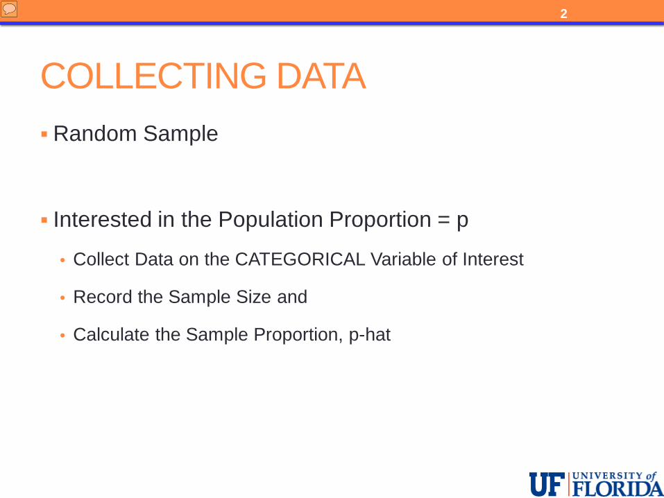
COLLECTING DATA Random Sample

Interested in the Population Proportion = p

• Collect Data on the CATEGORICAL Variable of Interest

• Record the Sample Size and

• Calculate the Sample Proportion, p-hat

2

We need to collect our data from a sample that is representative of the population about which we want to draw conclusions. 

Generally, the methods we are developing assume that the sample is chosen at random. The randomness is how we are able to apply the results from sampling distributions we developed earlier. 

Here we are working with hypothesis tests for a population proportion (p) so we will collect data on the relevant categorical variable from the individuals in the sample and calculate the sample proportion p‐hat. 

This is the natural quantity to calculate when the parameter of interest is p and now we have learned more about the behavior of this statistic, p‐hat from our discussion of sampling distributions. 

We will discuss calculating the test statistic as well as the conditions we need to check soon. 

For now, let’s go back to our three examples and add this step of calculating p‐hat to our figures.

2

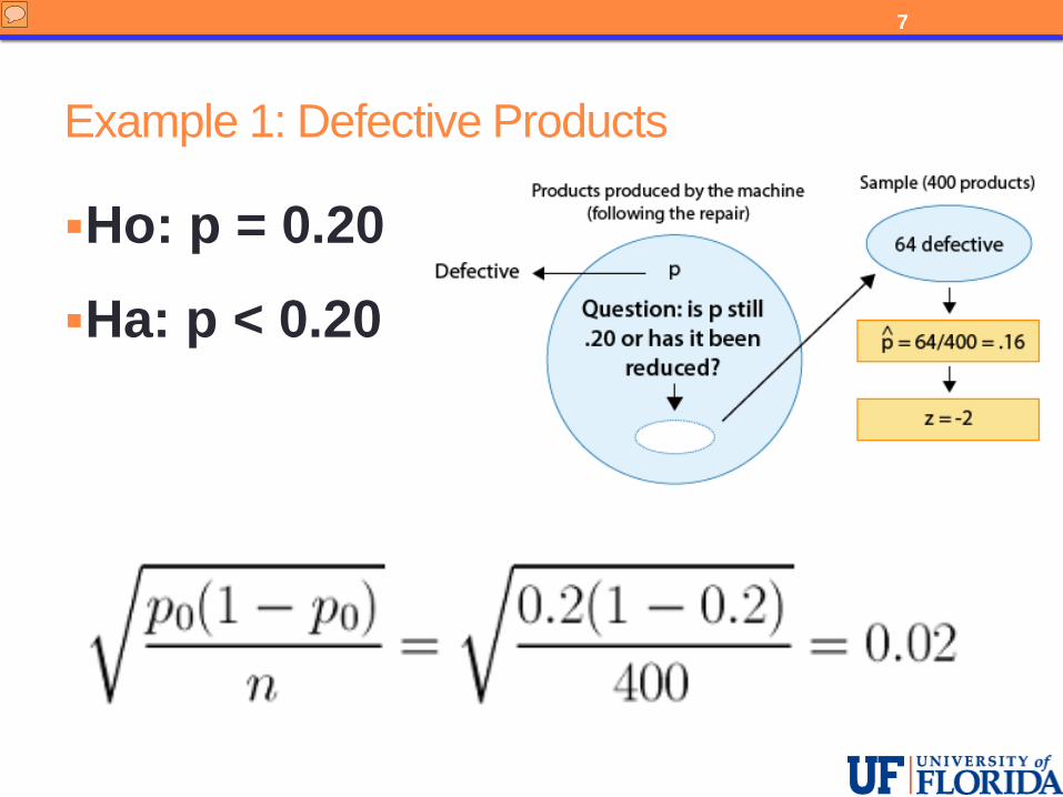
Example 1: Defective Products

Ho: p = 0.20

Ha: p < 0.20

3

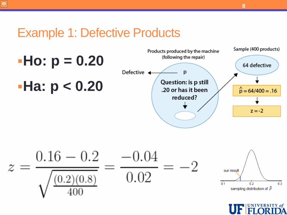
A machine is known to produce 20% defective products, and is therefore sent for repair. 

After the machine is repaired, 400 products produced by the machine are chosen at random and 64 of them are found to be defective. 

Do the data provide enough evidence that the proportion of defective products produced by the machine (p) has been reduced as a result of the repair?

The figure displays the information so far and adds the calculation of the sample proportion p‐hat which is 64 divided by 400 which is 0.16.

3

Example 2: Marijuana Use

Ho: p = 0.157

Ha: p > 0.157

4

There are rumors that students at a certain liberal arts college are more inclined to use drugs than U.S. college students in general. 

Suppose that in a simple random sample of 100 students from the college, 19 admitted to marijuana use. 

Do the data provide enough evidence to conclude that the proportion of marijuana users among the students in the college (p) is higher than the national proportion, which is 0.157? (This number is reported by the Harvard School of Public Health.)

The figure displays the information so far and adds the calculation of the sample proportion p‐hat which is 19 divided by 100 or 0.19.

4

Example 3: Death Penalty

Ho: p = 0.64

Ha: p ≠ 0.64

5

In 2003 a poll estimated that 64% of U.S. adults support the death penalty for a person convicted of murder. In a more recent poll, 675 out of 1,000 U.S. adults chosen at random were in favor of the death penalty for convicted murderers. 

Do the results of this poll provide evidence that the proportion of U.S. adults who support the death penalty for convicted murderers (p) changed between 2003 and the later poll?

The figure displays the information so far and adds the calculation of the sample proportion p‐hat which is 675 divided by 1000 which is 0.675.

Before moving on, notice that we did NOT use the information about p‐hat to help us set up our hypotheses. In practice the hypotheses are set up BEFORE we collect our data. 

In this course – the data is already provided which sometimes results in students using the information about p‐hat to incorrectly help them decide how to set up the hypotheses. 

We only used information about the overall question to help us set up the hypotheses in step 1. In this case, the question asked if there was a CHANGE – with no indication of the direction of the change. Even though our value is higher than the hypothesized value with our estimate of p‐hat of 0.675, our alternative hypothesis is still NOT EQUALS. 

5

TEST STATISTIC

6

We cannot look only at the difference between the sample proportion, p‐hat, and the null value, p0 because that would not take the variability of our estimator p‐hat into account. 

We know from our study of sampling distributions that this variation, called the standard error of p‐hat, depends on the sample size. Unfortunately, it depends upon the true value of p in the population which we do not know. 

In the case of hypothesis testing, since we start by assuming the null hypothesis is true, we use the value of p0 in our standard error equation. We need to do this instead of using p‐hat as the p‐value is calculated under the null distribution which assumes p0 is the true value of p. 

By “null distribution” we mean the distribution of the test statistic under the assumption that the null hypothesis is true. 

The test statistic is a standardized measure of how far the sample proportion p‐hat is from the null value p0, the value that the null hypothesis claims is the value of p. 

In other words, since p‐hat is what the data estimates p to be, the test statistic can be viewed as a standardized measure of the “distance” between what the data tells us about p and what the null hypothesis claims p to be.

Notice that in the numerator the value from the DATA comes first and our hypothesized value comes second. A common error is to swap the values in the numerator which can cause a serious error in your conclusions! 

A positive test statistic Indicates p‐hat is above p0  and a negative test statistic indicates p‐hat is below p0 .

Let’s return to our three examples. 

6

Example 1: Defective Products

Ho: p = 0.20

Ha: p < 0.20

7

In our defective products example, we have p‐hat = 0.16 and p‐zero = 0.20. 

Here we have shown the calculation of the null standard error used in the denominator of our z‐score. We must substitute the hypothesized value, not the value of p‐hat from our data. 

Here we get 0.2 times 1 minus 0.2 divided by 400 and then take the square root. In this case we get a value of 0.02. 

7

Example 1: Defective Products

Ho: p = 0.20

Ha: p < 0.20

8

To calculate the test statistic in this example we have z = in the numerator we have 0.16 minus 0.2 which is ‐0.04 and in the denominator we have the standard error we discussed on the previous slide which is 0.02. 

Dividing ‐0.04 by 0.02 we get a test statistic of z = ‐2. 

The sample proportion based upon this data is 2 standard errors below the null value.

8

Example 2: Marijuana Use

Ho: p = 0.157

Ha: p > 0.157

9

In our survey of college students about marijuana use, we have a p‐hat of 0.19 and a hypothesized value p‐zero of 0.157. 

Here we have the calculation of the test statistic resulting in Z = 0.91. 

We interpret this to mean that, assuming that Ho is true, the sample proportion p‐hat of 0.19 is 0.91 standard errors above the null value of 0.157.

9

Example 3: Death Penalty

Ho: p = 0.64

Ha: p ≠ 0.64

10

In our death penalty poll example, we have p‐hat = 0.675 and the hypothesized value, p‐zero of 0.64. 

Our test statistic is z = 2.31. 

We interpret this to mean that, assuming that Ho is true, the sample proportion p‐hat = 0.675 is 2.31 standard errors above the null value (0.64).

We can think about the test statistic as a measure of the evidence in the data against Ho. 

The larger the test statistic, the “further the data are from Ho” and therefore the more evidence the data provide against Ho.

10

CHECK CONDITIONS (i) Random Sample

(ii) Conditions under which the sampling distribution of p-hat is normal are met

11

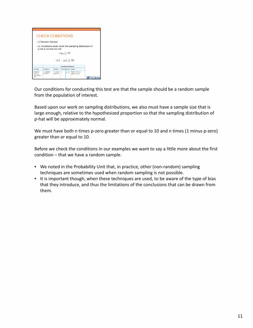
Our conditions for conducting this test are that the sample should be a random sample from the population of interest. 

Based upon our work on sampling distributions, we also must have a sample size that is large enough, relative to the hypothesized proportion so that the sampling distribution of p‐hat will be approximately normal. 

We must have both n times p‐zero greater than or equal to 10 and n times (1 minus p‐zero) greater than or equal to 10. 

Before we check the conditions in our examples we want to say a little more about the first condition – that we have a random sample. 

• We noted in the Probability Unit that, in practice, other (non‐random) sampling techniques are sometimes used when random sampling is not possible. 

• It is important though, when these techniques are used, to be aware of the type of bias that they introduce, and thus the limitations of the conclusions that can be drawn from them.

11

Can We Consider as “Random”?? Sample a LARGE ENGINEERING CLASS …

To study the proportion of students at a certain college who suffer from seasonal allergies

To study the proportion of students at a certain college who have math anxiety

12

One such practice is the situation in which a sample is not really chosen randomly, but in the context of the categorical variable that is being studied, the sample is regarded as random. • For example, say that you are interested in the proportion of students at a certain 

college who suffer from seasonal allergies. For that purpose, the students in a large engineering class could be considered as a random sample, since there is nothing about being in an engineering class that makes you more or less likely to suffer from seasonal allergies. 

• Technically, the engineering class is a convenience sample, but it is treated as a random sample in the context of this categorical variable. 

• On the other hand, if you are interested in the proportion of students in the college who have math anxiety, then the class of engineering students clearly could not possibly be viewed as a random sample, since engineering students probably have a much lower incidence of math anxiety than the college population overall.

Now let’s check the needed conditions for our examples. 

12

Example 1: Defective Products

Ho: p = 0.20

Ha: p < 0.20

13

Has the proportion of defective products been reduced as a result of the repair?i. The 400 products were chosen at random.

ii. n = 400, p0 = 0.2 and therefore:• n times p‐zero = 400 times 0.2 = 80 which is at least 10 and • n times 1‐ p‐zero = 400 times 1‐0.2 = 320 which is also at least 10. 

Therefore the conditions are satisfied to safely conduct this test. 

13

Example 2: Marijuana Use

Ho: p = 0.157

Ha: p > 0.157

14

Is the proportion of marijuana users in the college higher than the national figure?

i. The 100 students were chosen at random.

ii. n = 100, p0 = 0.157 and therefore:• n times p‐zero = 100 times 0.157 = 15.7 which is at least 10 and • n times 1 minus p‐zero = 100 times 1 – 0.157 = 84.3 which is at least 10

Therefore the conditions are satisfied to safely conduct this test. 

14

Example 3: Death Penalty

Ho: p = 0.64

Ha: p ≠ 0.64

15

Did the proportion of U.S. adults who support the death penalty change between 2003 and a later poll?

i. The 1000 adults were chosen at random.

ii. n = 1000, p0 = 0.64 and therefore:• n times p‐zero = 1000 times 0.64 = 640 which is at least 10 and • n times 1 minus p‐zero = 1000 times 1 – 0.64 = 360 which is at least 10

Therefore the conditions are satisfied to safely conduct this test. 

15

HYPOTHESIS TEST FOR ONE POPULATION PROPORTION – STEP 2

16

With respect to the z‐test for a population proportion that we are currently discussing we have:• Step 1: Completed• Step 2: Completed• Step 3: This is what we will work on next.

16