Hypersonic Heat Transfer and Anisotropic Visualization ... · Hypersonic Heat Transfer and...

Hypersonic Heat Transfer and Anisotropic Visualization with a

Higher Order Discontinuous Galerkin Finite Element Method

by

Douglas J. Quattrochi

B.S., Massachusetts Institute of Technology (2004)

Submitted to the Department of Aeronautics and Astronauticsin partial fulfillment of the requirements for the degree of

Master of Science in Aeronautics and Astronautics

at the

MASSACHUSETTS INSTITUTE OF TECHNOLOGY

June 2006

c© Massachusetts Institute of Technology 2006. All rights reserved.

Author . . . . . . . . . . . . . . . . . . . . . . . . . . . . . . . . . . . . . . . . . . . . . . . . . . . . . . . . . . . . . . . . . . . . . . . . . . . . . . . . . . .Department of Aeronautics and Astronautics

February 17, 2006

Certified by. . . . . . . . . . . . . . . . . . . . . . . . . . . . . . . . . . . . . . . . . . . . . . . . . . . . . . . . . . . . . . . . . . . . . . . . . . . . . . .David Darmofal

Associate ProfessorThesis Supervisor

Accepted by . . . . . . . . . . . . . . . . . . . . . . . . . . . . . . . . . . . . . . . . . . . . . . . . . . . . . . . . . . . . . . . . . . . . . . . . . . . . . .Jaime Peraire

Professor of Aeronautics and AstronauticsChair, Committee on Graduate Students

Hypersonic Heat Transfer and Anisotropic Visualization with a

Higher Order Discontinuous Galerkin Finite Element Method

by

Douglas J. Quattrochi

Submitted to the Department of Aeronautics and Astronauticson February 17, 2006, in partial fulfillment of the

requirements for the degree ofMaster of Science in Aeronautics and Astronautics

Abstract

Higher order discretizations of the Navier-Stokes equations promise greater accuracy thanconventional computational aerodynamics methods. In particular, the discontinuous Galerkin(DG) finite element method has O(hp+1) design accuracy and allows for subcell resolutionof shocks. This work furthers the DG finite element method in two ways. First, it demon-strates the results of DG when used to predict heat transfer to a cylinder in a hypersonicflow. The strong shock is captured with a Laplacian artificial viscosity term. On average,the results are in agreement with an existing hypersonic benchmark. Second, this work im-proves the visualization of the higher order polynomial solutions generated by DG with anadaptive display algorithm. The new algorithm results in more efficient displays of higherorder solutions, including the hypersonic flow solutions generated here.

Thesis Supervisor: David DarmofalTitle: Associate Professor

3

Acknowledgments

I often think clearly, but reason alone would have been insufficient to produce this thesis on

such a compressed timeline. Experience, too, was needed, and promptly shared with me at

my incessant requests by my collaborators in Project-X: Krzysztof Fidkowski, Todd Oliver,

and Garrett Barter. Enough cannot be said by way of appreciation for their alacritous and

enormously helpful advice, and for their work, of which this is a continuation. Similarly

crucial experience was shared by my advisor, David Darmofal, who knew enough about

CFD and project planning to answer my request for a hypersonics project with something

that would push against the limits of time and computational space; this is exactly how I

prefer to operate. Moreover, his precise and principled feedback was absolutely essential to

my education and to the compilation of this text. To Bob Haimes I owe a beautiful way to

describe my limited ability to use C pointers: “programming by Brownian motion.” I’d like

to think that in the course of our discussions some of his programming pizazz has rubbed off

on me. Also, I would be somewhat remiss not to mention J. Peter Whitney. From time to

time he would casually ask me how this work was going, and whatever I managed to grumble

at him, thwack it back with a startlingly incisive and fruitful question. I also acknowledge

Mike Park, whose generous consultations in the early stages of this work made possible the

acquisition of the Langley cylinder grid. And not least of all, I have benefitted greatly from

the experience of my parents, who were my first teachers, and who knew enough about

merit to fund nearly my entire education, and much else, no questions asked. It pleases me

to acknowledge this help beyond what may already appear in the footnotes or the references,

which is another long list, indeed.

A portion of this work was supported by NASA Langley under NAG-1-02037. This, last

but not least, is most gratefully acknowledged as well.

5

Contents

1 Introduction 13

1.1 The Origins of Blunt Body Computation . . . . . . . . . . . . . . . . . . . . . 13

1.2 The Search for Better CFD . . . . . . . . . . . . . . . . . . . . . . . . . . . . 14

1.3 Difficulties with Hypersonics . . . . . . . . . . . . . . . . . . . . . . . . . . . 15

1.4 Visualizing Higher Order Solutions . . . . . . . . . . . . . . . . . . . . . . . . 18

1.5 Contributions of this Thesis . . . . . . . . . . . . . . . . . . . . . . . . . . . . 19

2 Discontinuous Galerkin Method 21

2.1 Discretization of Navier-Stokes Equations . . . . . . . . . . . . . . . . . . . . 21

2.2 Newton Solver . . . . . . . . . . . . . . . . . . . . . . . . . . . . . . . . . . . 22

2.3 Shock Capturing . . . . . . . . . . . . . . . . . . . . . . . . . . . . . . . . . . 23

2.3.1 Previous Work . . . . . . . . . . . . . . . . . . . . . . . . . . . . . . . 24

2.3.2 Higher Order Artificial Viscosity . . . . . . . . . . . . . . . . . . . . . 25

2.3.3 Entropy Residual and Viscosity Model . . . . . . . . . . . . . . . . . . 25

3 Discontinuous Galerkin Results 29

3.1 Description of Problem . . . . . . . . . . . . . . . . . . . . . . . . . . . . . . . 29

3.1.1 Grid . . . . . . . . . . . . . . . . . . . . . . . . . . . . . . . . . . . . . 31

3.1.2 Boundary Conditions . . . . . . . . . . . . . . . . . . . . . . . . . . . 31

3.1.3 Langley Solution Techniques . . . . . . . . . . . . . . . . . . . . . . . 31

3.2 Discontinuous Galerkin Results . . . . . . . . . . . . . . . . . . . . . . . . . . 32

3.2.1 Grid . . . . . . . . . . . . . . . . . . . . . . . . . . . . . . . . . . . . . 32

3.2.2 Boundary Conditions . . . . . . . . . . . . . . . . . . . . . . . . . . . 32

3.2.3 Solution Technique . . . . . . . . . . . . . . . . . . . . . . . . . . . . . 34

7

3.2.4 The Overall Flow Field . . . . . . . . . . . . . . . . . . . . . . . . . . 35

3.2.5 Line Plots Through the Shock . . . . . . . . . . . . . . . . . . . . . . 35

3.2.6 The Flow Behind the Shock . . . . . . . . . . . . . . . . . . . . . . . . 39

3.2.7 Surface Plots . . . . . . . . . . . . . . . . . . . . . . . . . . . . . . . . 40

4 Visualization Method 51

4.1 Current Practice . . . . . . . . . . . . . . . . . . . . . . . . . . . . . . . . . . 51

4.2 Estimating the Error in a Display . . . . . . . . . . . . . . . . . . . . . . . . . 54

4.3 Display Refinement . . . . . . . . . . . . . . . . . . . . . . . . . . . . . . . . . 56

5 Visualization Results 63

5.1 Supersonic Inviscid Diamond Airfoil . . . . . . . . . . . . . . . . . . . . . . . 63

5.2 Subsonic Viscous Airfoil . . . . . . . . . . . . . . . . . . . . . . . . . . . . . . 67

5.3 Hypersonic Viscous Cylinder . . . . . . . . . . . . . . . . . . . . . . . . . . . 70

6 Conclusions 77

6.1 Discontinuous Galerkin Finite Element Method . . . . . . . . . . . . . . . . . 77

6.1.1 Remarks on DG for Hypersonics . . . . . . . . . . . . . . . . . . . . . 77

6.1.2 Future Work . . . . . . . . . . . . . . . . . . . . . . . . . . . . . . . . 77

6.2 Visualization . . . . . . . . . . . . . . . . . . . . . . . . . . . . . . . . . . . . 80

6.2.1 Comments on the Algorithm . . . . . . . . . . . . . . . . . . . . . . . 80

6.2.2 Future Work . . . . . . . . . . . . . . . . . . . . . . . . . . . . . . . . 80

8

List of Figures

1-1 Heat transfer results from the High Energy Flow Solver Synthesis . . . . . . . 17

3-1 The computational grid . . . . . . . . . . . . . . . . . . . . . . . . . . . . . . 30

3-2 Close-ups of the grids . . . . . . . . . . . . . . . . . . . . . . . . . . . . . . . 33

3-3 Contours of non-dimensional pressure, p/ρ∞V2∞, in 18 intervals from 0 to 0.9. 36

3-4 Density along stagnation streamline compared against benchmark . . . . . . 37

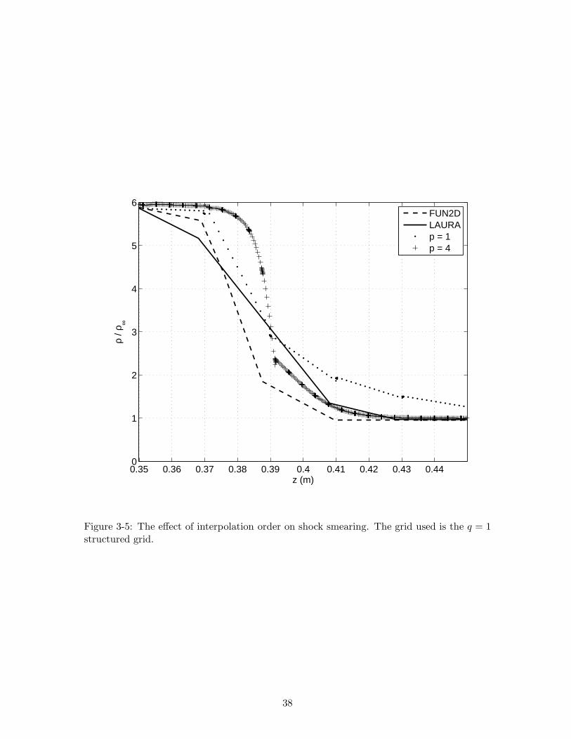
3-5 The effect of interpolation order on shock smearing . . . . . . . . . . . . . . . 38

3-6 Stagnation temperature variation, p = 2 . . . . . . . . . . . . . . . . . . . . . 39

3-7 Stagnation temperature variation, p = 4 . . . . . . . . . . . . . . . . . . . . . 40

3-8 Stagnation temperature line plots behind the shock showing oscillations . . . 41

3-9 Surface quantities, p = 1, q = 1 structured grid . . . . . . . . . . . . . . . . . 42



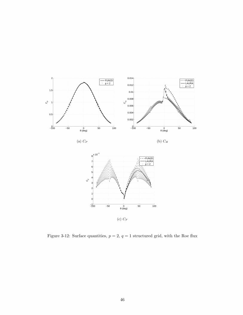
3-12 Surface quantities, p = 2, q = 1 structured grid, with the Roe flux . . . . . . 46

3-13 Surface quantities, p = 1, q = 1 partially unstructured grid . . . . . . . . . . . 47

3-14 Surface quantities, p = 2, q = 1 partially unstructured grid . . . . . . . . . . . 48


4-1 Uniform isotropic subdivision . . . . . . . . . . . . . . . . . . . . . . . . . . . 53

4-2 Reference and shadow elements for an original (computational) element . . . 56

4-3 The addition of a display node . . . . . . . . . . . . . . . . . . . . . . . . . . 56

4-4 Points evaluated for error . . . . . . . . . . . . . . . . . . . . . . . . . . . . . 57

4-5 Approximation of a curved computational element . . . . . . . . . . . . . . . 58

4-6 Locating a point in a grid . . . . . . . . . . . . . . . . . . . . . . . . . . . . . 60

9

5-1 Adaptive subdivision, diamond airfoil . . . . . . . . . . . . . . . . . . . . . . 64

5-2 Error as a function of display nodes for the M = 1.5 diamond airfoil grid . . 65

5-3 NACA airfoil . . . . . . . . . . . . . . . . . . . . . . . . . . . . . . . . . . . . 67

5-4 Error as a function of display nodes for the subsonic NACA airfoil grid . . . . 68

5-5 Contour plots of leading edge flow and entire flow, NACA airfoil, less refinement 71

5-6 Contour plots of leading edge flow and entire flow, NACA airfoil, more refine-

ment . . . . . . . . . . . . . . . . . . . . . . . . . . . . . . . . . . . . . . . . . 72

5-7 Examples of adaptive boundary layer refinement . . . . . . . . . . . . . . . . 73

5-8 Error as a function of display nodes for the hypersonic cylinder grid . . . . . 74

5-9 Hypersonic Display Grid, Uniform Isotropic . . . . . . . . . . . . . . . . . . . 75

5-10 Hypersonic Display Grid, Adaptive . . . . . . . . . . . . . . . . . . . . . . . . 75

6-1 Special consideration for higher order, high aspect ratio elements . . . . . . . 79

10

List of Tables

3.1 Test Case Flow Conditions . . . . . . . . . . . . . . . . . . . . . . . . . . . . 30

11

Chapter 1

Introduction

1.1 The Origins of Blunt Body Computation

A fundamental question in the design of any hypersonic flight vehicle is, “how hot will it

get?” The answer to this question usually motivates a follow-on, “how can it be prevented

from getting that hot?”

These two questions first received serious attention in the 1950’s from ballistic missile

designers [42]. When their slender, pointed missile designs were tested in hypersonic flows,

they invariably found the answer to the first question to be, “hot enough to melt.” Computers

were applied to the problem to find a survivable shape, but decades of experience in reducing

drag and streamlining vehicles had left the programmers trapped in the mindset “narrower is

better.” The answer always came back “make it narrower,” and the design always failed [33].

In 1952, National Advisory Committee for Aeronautics scientist H. Julian Allen, working

at the Ames Aeronautical Laboratory, realized that a blunted nose would fare far better in

high speed flight than the slimmest, sleekest missile designs at the time1 [1]. In fact, the heat

transfer to the nose of an object traveling much faster than the speed of sound is inversely

proportional to the square root of the radius of curvature [2]. So as a body is blunted and

its leading radius of curvature increased, the heat transfer to the body is decreased. Unlike

a pointed design, in which a shock sits on the body and the dissipated thermal energy is

transmitted directly to the vehicle, a blunted body forms a detached shock that redirects

enough of the thermal energy to the air flow for a heat sink to be effective.

1The work was set to paper with Alfred J. Eggers and remained classified until published six years later.

13

The so-called “blunt body” design became the best answer to the second question, but

in so doing considerably confused the answer to the first. Even for simple shapes, such as

cylinders or spheres, the flow around a blunt body has no analytical solution. The subsonic

flow found in the stagnation region, which is mathematically elliptic, can be analytically

coupled to the supersonic flow around it, which is mathematically hyperbolic, only if the

boundaries between the two regions are known in advance. Knowledge of the boundaries

comes only from the full solution.

The breakthrough came from computation. In 1966, Moretti and Abbett proposed ap-

plying computational techniques to the unsteady flow problem, which was everywhere hyper-

bolic [41]. With this approach, the unsteady problem converges to the steady-state solution,

with its supersonic and subsonic regions appearing automatically. Their original results were

consistent with the numerical data published at the time, as well as with analytical relations

for the change in state across a shock. While other specialized numerical methods had also

solved the “blunt body problem,” the Moretti and Abbett idea – solving a steady problem

with an unsteady computation – is generally applicable. It is used still, including in the

present work.

1.2 The Search for Better CFD

Since then a tremendous effort has been made to apply CFD to increasingly detailed and

difficult problems, hypersonic heat transfer being but one, and to produce increasingly ac-

curate results. The methods typically used in aerospace applications today are second-order

accurate, meaning that when solving smooth flow problems, as the grid spacing, h, decreases,

the error decreases as O(h2). For flows with shocks or other discontinuities, convergence will

be O(h).

Many modern CFD implementations were recently compared against one another and

against experiment in two workshops to predict the drag of a passenger jet in turbulent

flow [36, 39]. A sequence of three grids were used: one coarse, one medium, and one fine.

According to [36], “the medium grid was sized to be sufficient for industry drag prediction.”

The analysis of the results in [59] shows that the variation between implementations is sig-

nificant. Additionally, the sequence of grids could not be used to arrive at an asymptotically

14

grid-independent solution. The variation not only between methods but also between grids

casts doubt on whether industry’s O(h2) solutions are actually sufficient for industrial work.

The uncertainty of the results with industry-standard methods increases the allure of even

higher order discretizations as a means to achieve grid-independence with less computational

effort2. Higher order finite difference [37, 63, 68, 70] and finite volume [65] methods have

already been pursued. The salient problem with higher order accuracy in most of these

implementations is the extended coupling between grid points. This leads to problems with

stability, memory, and parallelization, and is discussed further in [19].

Discontinuous Galerkin (DG) finite element methods hold an advantage in this regard:

the ability to incorporate higher order accurate machinery entirely within an element. With

this discretization, the only coupling between grid elements comes from the inter-element

fluxes. This allows for the benefits of (at best) O(hp+1) accuracy [51], where p is the order of

the solution basis, without the problems of extended stencils. Explicit solution methods for

DG discretizations have been used to simulate the shocks found in hyperbolic problems [16],

as well as to simulate the boundary layers found in elliptic problems [6]. Implicit solution

methods have been developed more recently for DG discretizations of both hyperbolic and

elliptic problems [5, 19, 20, 21, 43].

1.3 Difficulties with Hypersonics

Long after Moretti and Abbett, the simulation of hypersonic flow fields of interest is still

difficult. The problems do not disappear with higher order methods.

At the most fundamental level, the physical models needed to describe the flow – for

instance, high temperature effects – remain case specific [18], or worse, poorly validated.

It is difficult to validate new models by comparing computation to experiment because of

experimental error, 3D effects in what appear to be 2D simulations [22], and the need to

compute flows not only in the test section but also throughout the entire facility [24, 66].

The most crucial of the problems with modeling is accurate prediction of the laminar-

turbulent transition [24, 66]. Without this, vehicles will continue to be severely overbuilt for

design conditions and in risk of failure when off-design. The example given in [66] is that

2In general, higher order means that the error decreases as O(h>1). “Even higher” order means higherthan those used in the drag prediction workshop, some of which were O(h2).

15

a 1mm uncertainty in the placement of protective tiling can lead to a 5 km uncertainty in

the altitude at which transition happens over the tile. Studies of transition and turbulent

heating in [7, 32] show how either laminar or turbulent heat transfer can be predicted to

within experimental accuracy, but the sometimes large transition region is not well modeled

at all. The error in transition heat transfer is as large as a factor of three.

Even with simplified physics, the implementation of a hypersonic flow model is still

problematic. Gnoffo lists three factors that have a large impact on the quality of a hypersonic

flow solution [24]. The first of these is grid alignment. A grid aligned well with a shock

produces less artificial dissipation than a badly aligned grid. This prevents the shock from

being smeared over many elements and reduces the amount of numerical error that washes

downstream. Good alignment may nevertheless aggravate a problem with certain fluxes,

particularly the Roe flux, that converge to spurious solutions in the presence of strong

shocks [22]. Possible fixes have been suggested in [26, 53].

The second factor is grid resolution. A grid should be finely resolved through shocks

and boundary layers. To keep the costs of a fine grid at a minimum, adaptive refinement

techniques, which generally require unstructured grids, should be used wherever possible [61].

The use of unstructured grids is consistent with another goal, namely, the ability to mesh

arbitrarily complex geometries. But adaptation is not without its own problems. In the

finite difference context, adaptation introduces spacing irregularities that may introduce

new errors [68]. It may also be that some degree of mesh orthogonality is required across a

shock [24], and for the calculation of surface gradients, regularity in the normal direction,

as well [14]. Such regularity and orthogonality are not achievable with fully unstructured

meshes, so it may be necessary to use prisms or other structured elements in conjunction

with unstructured elements.

The third factor is design order of accuracy. In the presence of a shock, discretizations

designed to be higher order accurate will be first order accurate. Subcell shock capturing

may reduce the effort required for a specific result [45], but even so remains first order

accurate. This first order error at shocks contaminates the solution globally, such that

adaptive control (through h and/or p) is required to realize the advantages of discretizations

with a high design order of accuracy. The global impact of errors at shocks is a particular

concern for aeroacoustics [12, 13].

16

(a) Heat transfer and pressure coeffi-cients. Different curves correspond todifferent span-wise locations.

(b) Contours of heat transfer coeffi-cient showing asymmetry in the stag-nation region.

Figure 1-1: Heat transfer results from the High Energy Flow Solver Synthesis, reproducedfrom [26].

Some of these difficulties are captured in the results of a recent application aimed at

predicting heat transfer on a cylinder. The method used was a 3D finite volume discretization

with a high temperature gas model [24, 26]. A semi-unstructured grid of tetrahedra was

used. It was produced by inserting diagonal faces into the hexahedra of a structured grid.

The diagonals were biased uniformly in one direction in an attempt to force an incorrectly

asymmetric solution. The tetrahedral mesh was used straight to the cylinder face, rather

than utilizing prismatic or hexahedral cells in the boundary layer.

Figure 1-1(a) shows the results for pressure and heat transfer across the front half of the

cylinder. There are ten curves for each quantity, one for each spanwise location, although the

pressure curves are so well aligned that they appear as one. The heat transfer, on the other

hand, shows significant spanwise asymmetry in the stagnation region. This is more apparent

in the contour plot of heat transfer across the cylinder face, Figure 1-1(b). The magnitude

of the asymmetry depended on the reconstruction algorithm used; the data displayed here

were generated with the best reconstruction tested. Gnoffo suggests in [26] that a fully

three-dimensional flux reconstruction would improve the results. He also suggests in [24]

that stagnation region heating estimates may be susceptible to entropy gradients produced

in the shock by mesh asymmetry. This example shows how sensitive heat transfer rates are

to the shock capturing algorithm and the choice of flux and reconstructions.

17

1.4 Visualizing Higher Order Solutions

Most visualization software packages calculate the solution to be displayed at a generic point

(x, y, z) in an element by linearly interpolating the solution given at the element’s nodes.

Even most software-hardware interfaces, such as OpenGL [44], are configured to deal with

linear display components. For piece-wise linear solutions, a linear display can be exact. For

solutions described by highly curved, higher order polynomials, however – particularly those

across shocks and boundary layers – the linear approximation may be very inaccurate.

The cost of inaccurate display is more than aesthetic. Depending on the magnitude of

the display errors, bad display can prompt one to false conclusions about stalled solutions,

about the numerical behavior of a simulation, or even about the physics of a problem. The

types of display errors most frequently encountered with linear displays are cataloged by

Buning in [10]. They include asymmetry of contour lines even on symmetric solutions,

incorrect streamlines resulting from the accumulation of integration errors, and orientation-

dependent (rather than solution dependent) shading within elements. A reliable visualization

package is essential as a user interface with CFD. A standard, unimproved linear display is

inadequate for higher order DG.

There are primarily two ways to improve the accuracy of a display for higher order

interpolated solutions. The first, pixel-exact rendering, lights each pixel according to the

solution at the pixel’s coordinates. This is used in [69] to follow higher order space-time DG

solutions by producing high quality videos. It has also been implemented with a modified

version of OpenGL for cutplanes through DG solutions in [9]. As the results show, pixel-

exact rendering produces remarkably clear displays. It tends to be on the slow side, however;

[69] achieves ten frames per second, and this is apparently with heavy emphasis placed on

observation rather than interactive probing. Visualization elements that are fully higher

order have been developed in [67], which also references work on higher order hexahedra,

higher order iso-surfaces (contours), and quadratic triangles. These are not strictly pixel-

exact methods, although they are exact for polynomial solutions up to the order of the

display element. They were designed for use with hierarchical data reduction methods,

which enable small workstations to view results so large they are computed and stored on

supercomputers. In this setting, higher order elements actually have a competitive advantage

18

in speed. They are much more efficient for transferring data between computers [67]. For

individual workstation rendering, however, they remain slower than linear elements.

The second method, linear subdivision, or polygonization, breaks each computational

element into a number of smaller, linear display elements. As the number of display el-

ements increases, the accuracy of the linear representation also increases. An error-based

polygonization algorithm is used to generate hierarchical surface meshes of 3D objects in [60].

Polygonization does not achieve the level of accuracy of a pixel-exact method, but it is fast.

Speed is an important consideration. The observations reported in [28] indicate that the

largest part of a user’s visualization time is spent probing and sampling flow field data. These

operations are slowed as the number of nodes increases. With too many nodes, interactivity

is reduced to a crawl. This can be just as crippling as an erroneous display. For example,

when a user must make mouse movements slowly so as not to overshoot the desired cursor

position, it quickly becomes tedious or impossible to extract data. Additionally, the lag time

is wasteful and disruptive to concentration.

The issue of speed with fully higher order visualization elements and pixel-exact methods

is not yet resolved. For this reason, the effort to improve the results of DG displays are

directed at better polygonization. The most straightforward way to make improvements

is to insert more linear subdivisions wherever the solution is not well approximated by the

current linear representation. The idea of display error estimation is the same as that of [67],

although the emphasis is on minimizing error rather than reducing data. Further discussion

of this topic is deferred until Chapter 4.

1.5 Contributions of this Thesis

The key result is a demonstration that a higher order DG discretization can be used to

simulate heat transfer in hypersonic flows with strong shocks.

Additionally, an error-based polygonization algorithm is implemented and demonstrated

to improve the efficiency of displaying higher order DG solutions while maintaining display

accuracy.

19

Chapter 2

Discontinuous Galerkin Method

2.1 Discretization of Navier-Stokes Equations

Following [43], the compressible, two-dimensional Navier-Stokes equations to model fluid

motion can be written in strong conservation form as

ut + ∇ · Fi(u) −∇ · Fv(u,∇u) = 0, (2.1)

where u is the conservative state vector,

u =(

ρ ρu ρv ρE)T

, (2.2)

Fi = (Fxi , Fy

i ) is the inviscid flux vector,

Fxi =

ρu

ρu2 + p

ρuv

ρuH

, Fyi =

ρv

ρuv

ρv2 + p

ρvH

,

ρ is the fluid density, u and v are the components of velocity in the x and y directions,

respectively, p is the pressure, H = E + p/ρ is the total enthalpy,

21

Fv = (Fxv , Fy

v) is the viscous flux vector,

Fxv =

0

23µ

(

2∂u∂x − ∂v

∂y

)

µ(

∂u∂y − ∂v

∂x

)

23µ

(

2∂u∂x − ∂v

∂y

)

u+ µ(

∂u∂y + ∂v

∂x

)

v + κ∂T∂x

,

Fyv =

0

µ(

∂u∂y − ∂v

∂x

)

23µ

(

2∂v∂y − ∂u

∂x

)

23µ

(

2∂v∂y − ∂u

∂x

)

v + µ(

∂u∂y + ∂v

∂x

)

u+ κ∂T∂y

,

µ is the dynamic viscosity, and κ is the thermal conductivity. The viscosity is calculated

using Sutherland’s Law, and κ = cpµ/Pr, where Pr is the gas Prandtl number and cp is the

specific heat at constant pressure.

These constitute four equations in five unknowns. The fifth required relationship is the

ideal gas equation of state, which when written in terms of the conserved quantities takes

the form

p = ρ(γ − 1)

(

E −(u2 + v2)

2

)

,

where γ is the ratio of specific heats.

The discretization of these equations is described in more detail in [21] and developed

fully in [43]. It proceeds from this strong form through the weak form and into the discrete

discontinuous Galerkin form. The viscous fluxes are discretized following the second Bassi

and Rebay scheme [5, 6].

2.2 Newton Solver

The system is discretized in time with the backwards Euler method, and the spatial residual

is linearized with respect to the current state vector. This yields a linear system for the

state update, ∆U ,(

1

∆tM +

∂R

∂U

)

∆U = −R(U), (2.3)

22

where M is the Mass matrix and R is the spatial residual. The solution is marched in

time with ∆t initially small to overcome transients and increased as the solution converges.

The linear system is solved with the aid of a preconditioned GMRES method [55]. The

preconditioner is the line solver described by Fidkowski, et. al. [21].

The solver, as well as the discretized form of the equations, are part of a discontinu-

ous Galerkin package currently being developed at the Aerospace Computational Design

Laboratory in the Department of Aeronautics and Astronautics at MIT [35].

2.3 Shock Capturing

The shocks that characterize supersonic flows of interest contain high frequency modes.

These modes may be dispersed by spatial discretizations that would be higher order accurate

on smooth, well-behaved problems1. The cause of this dispersion can be made clear through

examination of the modified partial differential equation, examples of which are given in

[3, 38] for the one-dimensional scalar advection equation. For higher Mach shocks these

dispersed waves appear as oscillations strong enough to prevent a solver from converging to

a stable solution. Special consideration is therefore required to simulate shocks with higher

order methods.2

There are two primary categories of shock simulation. The technique of “shock fitting”

is the most physically intuitive. The shock itself is treated as a computational boundary,

and the analytic Rankine-Hugoniot relations are used to link both sides of the shock [40]3.

Its disadvantage is its complexity to code for general shock shapes and motions, which are

not known in advance and must be calculated along with the solution.

The technique of “shock capturing” aims to allow stable shocks to arise without special

consideration given to their movement and position. In the following section, previous work

in shock capturing is reviewed.

1By practice and definition, the presence of the shock prevents these discretizations from being simplytermed “higher order accurate discretizations.” For brevity, the behavior of such discretizations on smoothproblems may be refered to as “design order of accuracy,” with a reference to this footnote.

2The subsequent subsections are derived from and anticipate the publication of the detailed work ofGarrett Barter, who is responsible for the shock capturing method used in this work.

3This was the method employed by Moretti and Abbett for the first blunt body calculation [41].

23

2.3.1 Previous Work

The first class of capturing methods was proposed by von Neumann [64]. The governing

partial differential equations are modified by the addition of a correction term that acts

as viscosity would, smearing dispersive discontinuities into non-dispersive regions of merely

large gradient. Besides smearing discontinuities, the artificial viscosity must meet three

requirements. First, it must scale like the resolution of a discretization, such that as the

resolution is increased the artificial viscosity can become arbitrarily small. Second, it must

be proportional to some indicator of the discontinuity, such that in smooth regions its effect

is negligible. Third, the Rankine-Hugoniot relations must still hold across the shock.

The second, more recent, class of capturing methods relies on the non-dispersive effects of

discretizations designed for first order accuracy4. In regions near shocks, the discretization

designed for higher order accuracy that is used elsewhere in the computation is replaced

with one designed to be only first order accurate or some hybrid between the two. The

replacement occurs typically in the numerical fluxes used, called “flux limiting” [8, 54], or

in the slopes of state variables, called “slope limiting” [56, 57, 58].

Limiting methods are currently used for explicit DG solvers on unsteady problems [11,

17, 34, 46, 47]. While the use of limiters can prevent oscillations, a trade-off exists between

monotonicity and convergence [62]. When the limiters are given a continuously differentiable

form, such that they eventually settle at fixed values throughout the flow, the solution

converges, but the shocks are no longer monotone. For an implicit, steady-state solution,

convergence is required, but shock monotonicity would be desirable, as well.

There is a more subtle uncertainty about limiting that makes it not readily adaptable to

higher order, implicit DG. When a solution is limited, the degrees of freedom are reduced.

In order to prevent the problem from becoming over-constrained, the constraints must be

reduced as well. The type of procedure required might be a continuously differentiable

reworking of the discrete jump from p = 1 to p = 0 described in [17]5. It is not clear how

best to accomplish this.

4See footnote 1.5Hereafter p is the solution polynomial order.

24

2.3.2 Higher Order Artificial Viscosity

Recently the artificial viscosity method has been applied to a higher order DG method

by Persson and Peraire to capture one-dimensional Mach 10 and two-dimensional Mach 5

shocks [45]. It satisfies the original von Neumann requirements, which give it one further

advantage. For a piecewise polynomial approximation, the resolution of a discretization

scales like h/p. The required artificial viscosity is thus O(h/p), and it is possible to capture

shocks with subcell resolution, rather than smearing them over several cells.

In the Laplacian form of the Persson and Peraire implementation, the artificial viscosity

is applied as an additional term in the Euler equations,

ut + ∇ · Fi(u) = ∇ · (ǫ∇u). (2.4)

The same approach is used here.

2.3.3 Entropy Residual and Viscosity Model

The Navier-Stokes equations with Laplacian artificial viscosity are written as

ut + ∇ · Fi(u) −∇ · Fv(u,∇u) = ∇ · (ǫ∇u). (2.5)

The implementation for this work differs from either the original von Neumann approach

or the Persson and Peraire approach in the way it identifies elements near shocks. Whereas

von Neumann used the gradient of a solution as a shock indicator, and Persson and Peraire

used resolution differences between solution orders, the present method indicates a shock

element by evaluating the production of entropy in that element. The exact entropy indicator

is formulated below.

By the definition of entropy,

ds ≡dQrev

T, (2.6)

the entropy of a fluid particle undergoing a reversible, adiabatic process is constant,

Ds

Dt= 0, (2.7)

25

or, considering a fixed point in space,

Ds

Dt=∂s

∂t+ ~v · ∇s = 0. (2.8)

For steady flow without dissipative effects, ~v · ∇s = 0 at every point in the flow field except

in a shock. For an element, e, containing a shock, the average entropy generation is detected

with the L1 integral over that element. The normalized L1 entropy residual for an element

is thus defined as

RS,e =k

δ

∫

eψ(~v · ∇s)dA = 0, (2.9)

where

δ =1

h

∫

eλsdA (2.10)

non-dimensionalizes the integral, λ = u + c is the maximum characteristic wave speed cal-

culated from quantities averaged over the element, c is the speed of sound, A is the element

area, k is a gain factor, and h = 4A/P is a characteristic length, where P is the element

perimeter. The function ψ is the absolute value function modified to remove the discontinuity

in the derivative, which would hinder convergence of the implicit solver.

ψ(x) ≡x2

|x| + ε, (2.11)

where ε is a constant O(0.1).

The artificial viscosity, ǫ, to be applied to each element is directly proportional to the

entropy residual,

ǫe = λh

p

RS,e

RS

, (2.12)

where p is the solution order, and RS is an expected entropy change,

RS =s2 − s1

12(s1 + s2)

. (2.13)

The subscripts 1 and 2 refer to positions before and after, respectively, a normal shock at

the average inflow Mach number. The expected entropy change is introduced to offset the

magnitude of RS,e, which is observed to be very large for strong shocks.

Even with the above normalization by RS , the amount of artificial viscosity added can be

26

extremely high at strong shocks. To limit the artificial viscosity, RS,e/RS is passed through

a smooth minimum function, xmin = min(x,C), defined as:

xmin =

C − 1a log(1 + exp(−a(x− C))) if xmin ≥ 0

0 if xmin < 0,

(2.14)

where a ≥ 0 is a smoothing constant. This form approximates the original min function

well for a = O(100). It also produces only positive output, but in doing so introduces a

discontinuity in the derivative for any x that cause y = 0. Assuming a = O(100), y = 0

occurs for positive x only with C < O(1 × 10−3). The discontinuity can thus be avoided in

practice. The capping values used with this function are given with the results.

Currently this entropy indicator is implemented for inviscid flow only. It has been used for

viscous heat transfer calculations by applying it only outside the boundary layers. Viscous

terms unrelated to shocks could be calculated with element viscous fluxes and removed from

the entropy residual, making it of general utility.

27

Chapter 3

Discontinuous Galerkin Results

The DG method is compared against a hypersonic benchmark published by the NASA labo-

ratory at Langley. Two finite volume codes were used for the benchmark, one structured and

one unstructured. The first is the Langley Aerothermodynamic Upwind Relaxation Algorithm

(LAURA). The second is the Fully Unstructured Navier-Stokes (FUN2D) code.

3.1 Description of Problem

The test case to be matched is the flow field around a right circular cylinder in a hypersonic

flow [15, 25]. The free-stream conditions are given in Table 3.1. The Reynolds number is

based on radius.

The publication of the original test case makes no mention of gas Prandtl number or

thermal conductivity. It is assumed that the gas Prandtl number is constant, Pr = 0.71.

Futhermore, the original test case did not specify whether viscosity was held at a constant

value consistent with the given Reynolds number or adjusted as a function of state. It is

assumed that the viscosity follows the Sutherland’s law dependence on temperature1,2.

29

Table 3.1: Test Case Flow Conditions

Value

V∞ 5000 m/sρ∞ 0.001 kg/m3

T∞ 200 KM∞ 17.605Re 376, 930γ 1.4

Pr 0.71

Twall 500K

Outflow Outflowx (m)

z(m

)

-2 -1 0 1 2-1

-0.5

0

0.5Inflow

Cylinder

Figure 3-1: The computational grid.

30

3.1.1 Grid

The computational grid developed for the benchmark by Langley is shown in Figure 3-

1. It is formed by creating a structured quadrilateral mesh around a cylinder of radius

1m and cutting the quadrilaterals into triangles so as to uniformly bias the direction of

the diagonals. This asymmetry makes for a difficult test case, as it may result in falsely

asymmetric solutions. The computational domain is sufficiently large and refined to allow

for resolution of both the detached bow shock and the viscous boundary layer using the

LAURA code. Nodes near the inflow boundary have been aligned with the shock by means

of the LAURA “align-shock option.” The grid is 65 nodes normal to the body by 61 nodes

circumferentially.

3.1.2 Boundary Conditions

As described in Section 2.1, the gas is modeled as thermally and calorically perfect. The

free-stream is uniform and directed in the −z-direction. The cylinder surface is a “no slip”

boundary at a constant temperature of Twall = 500 K. Where the flow moves past either side

of the cylinder and exits the computational domain, the FUN2D code uses an extrapolation

boundary condition. The LAURA exit condition here is not specified but is presumed to be

the same.

3.1.3 Langley Solution Techniques

Both Langley solutions were initialized to free-stream conditions. For robustness each so-

lution proceeded in two steps. The FUN2D code was initially run with first-order accurate

fluxes and after some iterations was run with second-order accurate fluxes. Convergence was

determined by skin friction rather than the L2 error norm, which was observed to stall. The

LAURA code was first run with point-implicit relaxation and after some iterations was run

with line-implicit relaxation.

1The close match of the presented results (below) with those already published, and the disparity betweenconstant viscosity results and those published, appears to support this assumption.

2Sutherland’s law is physically accurate for much of the boundary layer, and certainly for the thin, cooledregion near the body [52].

31

3.2 Discontinuous Galerkin Results

3.2.1 Grid

The DG method is applied with three different grids. The first is the exact Langley grid

with a linear representation of the cylinder surface, q = 1. The second is basically the same

but with a quadratic, q = 2, description of the cylinder surface3. The higher order geometry

is used following the observations of Bassi and Rebay, which suggest that superparametric

elements are required with DG [4]. The third grid keeps the first 40 rows of elements in

the boundary layer, but replaces the elements across the shock with badly aligned, fully

unstructured elements. This grid will be refered to as the “partially unstructured” grid.

Portions of both the structured and partially unstructured grids are shown in Figure 3-2 for

comparison. The partially unstructured grid contains 60% more nodes than the structured

grid; the primary purpose is to test the effect of shock-aligned elements on downstream flow

properties.

3.2.2 Boundary Conditions

The exact Langley boundary conditions are matched. From the parameters given in Table 3.1

the full state vector, Equation (2.2), is calculated and specified along the inflow boundary

(Figure 3-1). The cylinder surface is modeled with a “no slip” condition and a constant wall

temperature of 500 K. At the outflow boundaries an extrapolation boundary condition

is applied. The inviscid fluxes are calculated using state data from the interior of the

grid. The three viscous boundary terms in the Bassi and Rebay 2 discretization for the

artificial viscosity are set to zero because there is no artificial viscosity associated with the

boundaries [5, 6]. Although the inviscid extrapolation boundary condition is observed to

be generally unstable when the exiting flow is subsonic, the boundary layers do not cause

stability problems except for low Re initial transients (see Section 6.1.2 on initialization).

3The q = 2 geometry is actually used to describe every element in the grid. See Section 6.1.2 on gridgeneration.

32

x

z

0 0.5 1 1.5-1

-0.5

0

0.5

(a) The partially unstructured grid, with elements misaligned withthe shock.

x

z

0 0.5 1 1.5-1

-0.5

0

0.5

(b) The original structured grid

Figure 3-2: Close-ups of the grids

33

3.2.3 Solution Technique

The present DG method cannot converge a piecewise linear or higher (p ≥ 1) solution when

the flow field is initialized to free-stream conditions because a strong shock forms along the

body and oscillations around the shock grow without bound. This is observed regardless of

the amount of artificial viscosity added with the artificial viscosity model (Section 2.3.3).

These oscillations are at first not visible in the conserved state vector quantities themselves,

which when viewed independently appear to be normal. Rather, they first appear in com-

binations of conserved variables. For instance, pressure, (2.1), approaches zero, and Mach

number increases by orders of magnitude. The problem is most often observed along the

stagnation line, although with varied input and time stepping it can be made to occur in

a number of places along the shock, usually symmetric with respect to the stagnation line.

The present method can converge a piecewise constant (p = 0) solution from initialization

at free-stream conditions. Nevertheless, a converged p = 0 solution cannot be used as a

starting point for a p = 1 solution because the same instability returns. This again seems to

be true regardless of attempts to stabilize the shock with the artificial viscosity model.

It may be possible to avoid either of these two difficulties with more careful consideration

given to finding a stabilizing cap and gain (defined in Section 2.3.3). For this work, however,

a two-step solution procedure was found to be the most robust. The first step is to solve an

“easier” problem on the target grid, for example, M = 10, Re = 10, 000, p = 0, initialized

to free-stream conditions. The second step is to restart from this converged p = 0 solution

while simultaneously increasing M, Re, and p. This establishes a transient p = 1 solution at

the weaker, lower Mach shock, around which oscillations are manageable, before the higher

Mach flow moves in from the boundary. From this converged p = 1 solution all higher order

interpolations will converge at high Mach number.

The inviscid fluxes for these results are calculated using the Lax-Friedrichs flux. The

Roe flux is observed to carbuncle at p = 0 [48]. The carbuncle cannot be used as an initial

condition for a higher p solution with either flux. With a valid p = 0 solution, on the other

hand, i.e., the Lax-Friedrichs solution, either flux can be used for higher p solutions. In the

latter case, the Roe flux requires more artificial viscosity (results below). Unless otherwise

noted, all data is presented for the Lax-Friedrichs flux.

34

3.2.4 The Overall Flow Field

Figures 3-3 show the entire flow field in a contour plot of non-dimensionalized pressure, which

ranges from 0 to 0.9 over 18 contours in each subfigure. The DG second order accuracy result

on the structured q = 1 grid is in good qualitative agreement with the Langley codes. The

result is visibly identical on the structured q = 2 grid (not shown) and very similar on the

partially unstructured q = 1 grid, Figure 3-3(c).

3.2.5 Line Plots Through the Shock

Figure 3-4 compares the solutions of each of the three codes in a plot of density ratios

along the stagnation line4. The DG results here are shown with the design O(h2) accurate

discretization, p = 1, to match the design order of the FUN2D and LAURA discretizations5.

The cylinder is at z = 0 m. The empirically determined cap and gain on the entropy

indicator required to stabilize the shock, C = 1.75 and k = 0.3, (Section 2.3.3), were used

for the q = 1 structured grid, and C = 1.75, k = 0.4 were used for the partially unstructured

grid6. Three points are sampled in each element. The shock is smeared across approximately

eight elements and appears monotone. The results are in good agreement with the Langley

results.

Figure 3-5 examines the effect of increasing p on the resolution of the shock with the

q = 1 structured grid, now displayed with 15 evenly distributed points per element. Both

the p = 1 and p = 4 cases are run with the same gain on artificial viscosity, so as p increases,

the artificial viscosity is reduced (Equation 2.12). The result is a visible sharpening of the

shock at p = 4, for which the shock is smeared over only three elements. Although the p = 4

solution does not display the sub-cell shock capturing demonstrated by Persson and Peraire,

they note a similar result for their Laplacian artificial viscosity method: it appears to result

in wider shocks than the use of a model based on the physical dissipation of an ideal gas.

The two methods are compared in [45].

4For all line plots, the Langley benchmark results displayed are the averages of the nearest cell centers.5As mentioned previously, all discretizations are only O(h) with shocks.6The density behind the shock is on average too low if k = 0.4 is used with the structured grid; this is

because the shock is smeared too far forward. The difference in k is just a result of the order in which k wastried, it being adjusted only for unconverged or unsatisfactory solutions.

35

(a) Langley FUN2D and LAURA

x (m)

z(m

)

-2 -1 0 1 2-1

-0.5

0

0.5

(b) Discontinuous Galerkin p = 1, q = 1 structured grid

x (m)

z(m

)

-2 -1 0 1 2-1

-0.5

0

0.5

(c) Discontinuous Galerkin p = 1, q = 1 partially unstructured grid

Figure 3-3: Contours of non-dimensional pressure, p/ρ∞V2∞, in 18 intervals from 0 to 0.9.

36

0 0.05 0.1 0.15 0.2 0.25 0.3 0.35 0.4 0.45 0.50

1

2

3

4

5

6

7

8

9

10

z (m)

ρ / ρ

∞

FUN2DLAURAstructuredunstructured

Figure 3-4: Density along stagnation streamline compared against benchmark. The solutionis p = 1 on the q = 1 structured and partially unstructured grids.

37

0.35 0.36 0.37 0.38 0.39 0.4 0.41 0.42 0.43 0.440

1

2

3

4

5

6

z (m)

ρ / ρ

∞

FUN2DLAURAp = 1p = 4

Figure 3-5: The effect of interpolation order on shock smearing. The grid used is the q = 1structured grid.

38

x

z

-1 -0.5 0 0.5 1-1

-0.8

-0.6

-0.4

-0.2

0

0.2

0.4

0.6

0.8

1

Figure 3-6: Stagnation temperature variation behind shock, Tt/Tt∞, in 100 contours between0.04 and 1.05; p = 2, q = 1 structured grid.

3.2.6 The Flow Behind the Shock

Figures 3-6 and 3-7 show contour plots of stagnation temperature behind the shock, with 100

intervals between the minimum and maximum flow field values. These are clearly asymmetric

in both cases, with greater asymmetry at lower p.

Figures 3-8 show line plots of stagnation temperature, normalized by the free-stream

value, from approximately (0.5, 0.2) to (−0.5, 0.2), which is a line behind the shock and

perpendicular to the direction of the free-stream, for p = 2 and p = 4. The asymmetry

is more pronounced for lower p. The graphs are clearly oscillatory, whereas the inflow

conditions are not. These oscillations are larger with higher p. The results shown for

p = 4 produced with cap and gain on the shock entropy indicator of C = 1.75 and k = 0.4

correspond to a peak artificial viscosity in the shock along the stagnation line of ǫe = 8×10−3.

Alternatively caps of C = 2.75 and C = 1 were tried, for peak artificial viscosities along

the stagnation line of 11 × 10−3 and 4 × 10−3. The magnitude of the largest oscillation is

approximately 33% lower for ǫe = 8 × 10−3 compared with ǫe = 4 × 10−3, although the

oscillations are the same size for ǫe = 4×10−3 and ǫe = 11×10−3, so no trend with artificial

39

x

z

-1 -0.5 0 0.5 1-1

-0.8

-0.6

-0.4

-0.2

0

0.2

0.4

0.6

0.8

1

Figure 3-7: Stagnation temperature variation behind shock, Tt/Tt∞, in 100 contours between0.04 and 1.05; p = 4, q = 1 structured grid.

viscosity is apparent7. These oscillations may have an effect on the surface quantities (see

below), which are also oscillatory, although causality is not clear; the region of these line

probes is subsonic, so the oscillations could be caused by, rather than the cause of, something

downstream. It seems most likely, however, that they are the result of oscillations in the

captured shock.

3.2.7 Surface Plots

The q = 1 structured grid is considered first. Plots of surface pressure coefficient, heat

transfer coefficient, and skin friction coefficient are shown for three different p in Figures 3-

9, 3-10, and 3-11 as a function of angle measured from the stagnation line (θ > 0 corresponds

to x > 0)8. The LAURA pressure coefficient is very nearly the FUN2D pressure coefficient,

so only one is shown.

The salient feature of these surface quantities is the discontinuous jump in the solution

between each element. To some extent this is expected because DG allows for these jumps.

The oscillations are also, to some extent, expected as a result of the linear geometry, which

7Time constraints prevented a more thorough investigation.8p = 4 was also tested and is very similar to p = 3

40

0 0.2 0.4 0.6 0.8 1 1.20.97

0.98

0.99

1

1.01

1.02

1.03

1.04

1.05

T0/ T

0,∞

Distance from (0.5, 0.2)

(a) Stagnation temperature line plot p = 2

0 0.2 0.4 0.6 0.8 1 1.20.97

0.98

0.99

1

1.01

1.02

1.03

1.04

1.05

T0/ T

0,∞


(b) Stagnation temperature line plot p = 4,C = 2.75

0 0.2 0.4 0.6 0.8 1 1.20.97

0.98

0.99

1

1.01

1.02

1.03

1.04

1.05

T0/ T

0,∞


(c) Stagnation temperature line plot p = 4,C = 1.75

0 0.2 0.4 0.6 0.8 1 1.20.97

0.98

0.99

1

1.01

1.02

1.03

1.04

1.05

T0/ T

0,∞


(d) Stagnation temperature line plot p = 4,C = 1.0

Figure 3-8: Stagnation temperature line plots behind the shock showing oscillations, q = 1structured grid.

41

−100 −50 0 50 1000

0.5

1

1.5

2

θ (deg)

CP

FUN2Dp = 1

(a) CP

−100 −50 0 50 1000

0.002

0.004

0.006

0.008

0.01

0.012

0.014

θ (deg)

CH

FUN2DLAURAp = 1

(b) CH

−100 −50 0 50 100−1

0

1

2

3

4

5

6

7

8x 10

−3

θ (deg)

CF

FUN2DLAURAp = 1

(c) CF

Figure 3-9: Surface quantities, p = 1, q = 1 structured grid

42

−100 −50 0 50 1000

0.5

1

1.5

2

θ (deg)

CP

FUN2Dp = 2

(a) CP

−100 −50 0 50 1000

0.002

0.004

0.006

0.008

0.01

0.012

0.014

θ (deg)

CH

FUN2DLAURAp = 2

(b) CH , spike reaches ≈ 1.75 × 10−3

−100 −50 0 50 100−1

0

1

2

3

4

5

6

7

8x 10

−3

θ (deg)

CF

FUN2DLAURAp = 2

(c) CF


43

−100 −50 0 50 1000

0.5

1

1.5

2

θ (deg)

CP

FUN2Dp = 3

(a) CP

−100 −50 0 50 1000

0.002

0.004

0.006

0.008

0.01

0.012

0.014

θ (deg)

CH

FUN2DLAURAp = 3

(b) CH

−100 −50 0 50 100−1

0

1

2

3

4

5

6

7

8x 10

−3

θ (deg)

CF

FUN2DLAURAp = 3

(c) CF


44

introduces a radial error in the position of the cylinder face and discontinuities in the slope

between faces. It is expected that for higher p, both the interelement jumps and oscillations

will be reduced. This is observed with pressure, which quickly becomes consistent with

the FUN2D line and the LAURA line (not shown, nearly the same as FUN2D), as well as

with the modified Newtonian pressure coefficient [2]. For the skin friction, however, the

oscillations are not reduced, but rather appear to worsen. For the heat transfer, the p = 2

solution is worse than the p = 1 solution, but p = 3 spikes less than p = 2.

The Roe flux was used to calculate a p = 2 solution on the same grid. Whereas the Lax-

Friedrichs flux used a cap and gain as small as C = 1.75, k = 0.4, the Roe flux required more;

values of C = 5, k = 1.2 were used, although no attempt was made to find the minimum

required. The results, no better than the Lax-Friedrichs results, are shown in Figure 3-12.

Figure 3-13 shows the p = 1 solution on the q = 1 partially unstructured grid. The

only significant difference between the input for this test and the p = 1 test on the q = 1

structured grid is the alignment of elements across the shock. Here they are not well aligned.

Comparison of the two heat transfer graphs, Figure 3-13(b) and Figure 3-9(b), show that this

makes a difference, of the order of the jumps between elements. This supports the suggestion

made by Gnoffo in [24] that errors in the shock capturing caused by a poorly aligned grid can

wash downstream and affect stagnation region heating estimates. This is the most plausible

explanation for the difference, as the boundary layer gridding and simulation conditions are

otherwise equal between this case and the structured one. Figure 3-14 shows p = 2 results

on the same q = 1 unstructured grid. In this case, the unstructured results for heat transfer

look better than the structured results. The results are similar for p = 3 (not shown).

Figure 3-15 shows the the p = 2 solution on a q = 2 grid, for which every element is

described by higher order geometry, see Section 6.1.2, grid generation. Higher order geometry

does not improve the solution to the extent that would be expected, except for the pressure

curve, which is very smooth. The q = 2 geometry appears not to improve, however, the

skin friction and heat transfer results. The conclusions drawn from these results are given

in Section 6.1.

45

−100 −50 0 50 1000

0.5

1

1.5

2

θ (deg)

CP

FUN2Dp = 2

(a) CP

−100 −50 0 50 1000

0.002

0.004

0.006

0.008

0.01

0.012

0.014

θ (deg)

CH

FUN2DLAURAp = 2

(b) CH

−100 −50 0 50 100−1

0

1

2

3

4

5

6

7

8x 10

−3

θ (deg)

CF

FUN2DLAURAp = 2

(c) CF

Figure 3-12: Surface quantities, p = 2, q = 1 structured grid, with the Roe flux

46

−100 −50 0 50 1000

0.5

1

1.5

2

θ (deg)

CP

FUN2Dp = 1

(a) CP

−100 −50 0 50 1000

0.002

0.004

0.006

0.008

0.01

0.012

0.014

θ (deg)

CH

FUN2DLAURAp = 1

(b) CH

−100 −50 0 50 100−1

0

1

2

3

4

5

6

7

8x 10

−3

θ (deg)

CF

FUN2DLAURAp = 1

(c) CF

Figure 3-13: Surface quantities, p = 1, q = 1 partially unstructured grid

47

−100 −50 0 50 1000

0.5

1

1.5

2

θ (deg)

CP

FUN2Dp = 2

(a) CP

−100 −50 0 50 1000

0.002

0.004

0.006

0.008

0.01

0.012

0.014

θ (deg)

CH

FUN2DLAURAp = 2

(b) CH

−100 −50 0 50 100−1

0

1

2

3

4

5

6

7

8x 10

−3

θ (deg)

CF

FUN2DLAURAp = 2

(c) CF

Figure 3-14: Surface quantities, p = 2, q = 1 partially unstructured grid

48

−100 −50 0 50 1000

0.5

1

1.5

2

θ (deg)

CP

FUN2Dp = 2

(a) CP

−100 −50 0 50 1000

0.002

0.004

0.006

0.008

0.01

0.012

0.014

θ (deg)

CH

FUN2DLAURAp = 2

(b) CH

−100 −50 0 50 100−1

0

1

2

3

4

5

6

7

8x 10

−3

θ (deg)

CF

FUN2DLAURAp = 2

(c) CF


49

Chapter 4

Visualization Method

4.1 Current Practice

The higher order interpolation solutions generated with this DG method are visualized with

the Visual3 display package [28, 29, 30, 31]. Visual3 takes as input a list of grid node

coordinates, connectivity data linking those nodes into elements, and solution data at each

node. It displays a solution by linear Gouraud shading between nodes [27].

The accuracy of the linear approximation to the higher order solution is currently im-

proved by uniform, isotropic1 subdivision of each computational element into a number of

smaller display elements. The number of subelements in the current method is nd, where d is

the problem dimensionality (2 or 3) and n is the larger of the solution interpolation order, p,

or the geometry interpolation order, q. This method is simple to implement. A polynomial

solution in any basis can be converted to the nodal Lagrange basis, which uses as its weights

the solution at the nodes of an isotropic subdivision of pd elements. For q = 1 elements, the

Lagrange data is copied directly to Visual3. For q > 1 elements, the same number of points

are sampled, nd, but the points are evenly spaced over the curved element. Overall the pro-

cedure is simply a matter of sampling the solution at some points and copying the data to

Visual3. But this method has two disadvantages. First, it provides no guarantee of display

accuracy. Second, it introduces nodes independent of the quality of the display, resulting in

additional nodes where the linear display was already adequate. This extra computational

expense slows user interactivity with the visualization software.

1Or best approximation, for tetrahedra.

51

Consider the two-dimensional (2D) M = 1.5 flow over a diamond airfoil approximated

by piece-wise fifth-order polynomials on a grid with 212 discontinuous elements. The min-

imum display grid has 636 = 212 × 3 nodes2, Figure 4-1(a). Figure 4-1(b) shows contours

of non-dimensional density, ρ/ρ∞, with 10 contour levels in increments of 0.04 using the

computational grid as the display grid. Figure 4-1(d) shows the same contours, but using

the grid in which each computational element is isotropically subdivided into 25 display

elements (Figure 4-1(c)).

The leading and trailing edge shocks are visible without subdivision, but the expansion

fan is completely lost. On the other hand, the uniform isotropic subdivision correctly displays

the expansion fan, but there are now 4452 = 212× 21 nodes in the display grid (an increase

of 700%). Approximately seventy of the computational elements are ahead of the leading

shock, where the flow is uniform, so that approximately 1260 = 70× (21− 3) nodes inserted

above the minimum number required are not adding any new information to the display.

This is more than a quarter of the nodes added for this problem.

The excess is compounded in 3D, as each computational element is subdivided into n3

display elements. On an Intel Pentium 4, 2.53 GHz processor with 512 MB RAM it takes

approximately 16 seconds to load a 3D grid with 50,000 q = 1 elements and a p = 1 solution,

where no refinement is called for. More importantly than load time, the size of the display

is sufficiently large to cause noticeable lag between action and response when probing the

data.

The trade-off is between accuracy and efficiency. A more efficient way to display results

would be to add points only when needed, and to keep adding points until the linearly

displayed solution resembles the computed higher order solution to within some desired

accuracy. This requires better preprocessing, but leaves intact the core of Visual3, which

has proved itself to be a fast and reliable research tool. The first step in this preprocessing

is accurately assessing the error in a display.

2A note on node counting: The nodes joining computational elements become different but overlappingdisplay nodes for DG visualization because solution data is discontinuous across elements. The minimumnumber of display nodes for an unstructured DG grid is thus considered to be ne(d + 1), where ne is thenumber of elements. When additional nodes are inserted for the purpose of display, however, they connectsubelements within a single computational element. Thus the solution data, and therefore nodes, are sharedbetween subelements. For a p = 5 solution, isotropic subdivision results in 21 nodes per element.

52

x

y

-3 -2 -1 0 1 2 3-3

-2

-1

0

1

2

3

(a) Computational grid as display grid

xy

-3 -2 -1 0 1 2 3-3

-2

-1

0

1

2

3

(b) Linear display on computational grid

x

y

-3 -2 -1 0 1 2 3-3

-2

-1

0

1

2

3

(c) Uniformly, isotropically refined displaygrid

x

y

-3 -2 -1 0 1 2 3-3

-2

-1

0

1

2

3

(d) Linear display on refined display grid

Figure 4-1: Uniform isotropic subdivision; contours are of ρ/ρ∞ in 10 levels from 0.84 to 1.2

53

4.2 Estimating the Error in a Display

The error of a display depends on the magnitude of the difference between the higher order

solution, u, and the linear interpolation between nodes, uL. A standard norm that can be

used to evaluate the error is

La(v) = ||v||a =

[∫

Ω

|v|adΩ

]1/a

, (4.1)

where a is the measure of the norm and Ω can be the element edges l, faces f , or interiors i

in a grid, and v is the function being measured. The norms used here are the L1 and L∞ of

the display error,

||u− uL||1 =

∫

Ω

|u− uL|dΩ,

||u− uL||∞ = maxΩ

|u− uL|.

Rather than calculate the L∞ norm, it is approximated as

||u− uL||∞ ≈ maxc

|u(xc) − uL(xc)| = ||u− uL||c∞, (4.2)

where xc are a set of sampling points3. The set of sampling points, c, are chosen as the

union of the sets of quadrature points on element interiors, i, edges, l, and faces (in 3D)

that would exactly integrate the piecewise polynomial error of a conserved state variable4.

This work considers only the 2D case and presents L1-type error results for the grid interior

only.

For consistent application of these global error estimates across different grids, they are

3An optimization problem might be solved to find the true L∞ norm, although this has not been pursuedfor this work.

4Although combinations of state variables, such as Mach number and pressure, can be used as an errorindicator, they will not in general be polynomial of the same degree as the solution order. This would affectthe choice of quadrature rule used to approximate the integrals if a certain accuracy was desired.

54

non-dimensionalized:

E1 =||u− uL||1

||u||1,

E∞ =1

||u||imax

1 /Aimax

maxl,i

|u− uL|.

The local pointwise error used to direct node insertion (see below) is normalized by local

quantities5. The global E∞ estimate is non-dimensionalized in the same way to be consistent

with the estimate controling node insertion; here imax is the element in which this global

error occurs, and Aimax the area of this element. This non-dimensionalization will not be

reliable if the average value of the state variable chosen is zero for an element. Alternatively,

if a user cannot find a state variable that is, on average, never zero, the dimensional forms

of the error estimates can be used.

The L1 norm is approximated using a higher-order quadrature rule on the computational

element. The solution basis, φ, for a computational element is polynomial of degree p in the

physical space, even when the elements are curved. This is ensured by defining the solution

basis on the linear shadow reference element, rather than on the physical element [21]. The

shadow element is formed by connecting the vertices of the element with straight lines, see

Figure 4-2, and its reference is a rotation and stretching of the shadow into convenient

coordinates. To sample the solution at a physical point, xc, its coordinates are mapped to

the shadow reference space. The locations of xc, however, are first mapped from locations,

ξc, in a reference element, which in 2D has vertices (0, 0), (1, 0), (0, 1), because this is where

the quadrature point locations are defined. Thus the discrete form of an area integral is

∫

ef(φ)dx =

∑

g

wgf(φ(B−1A(ξg)))|J|, (4.3)

where f is the function to be evaluated, φ are the basis functions on the shadow reference

element, wg is the weight of quadrature point g, J is the Jacobian of the mapping from

the reference element to the physical element, and A and B−1 are the mappings between

elements shown in Figure 4-2.

5This gives something closer to a pointwise percent error than normalization by ||u||1 over the entire grid.

55

ξ

ξ

x

x

A

B

B

1

2

-1

1

2

ξ1

ξ2’

’

Reference element Shadow reference element

Original element (solid)Shadow element (dashed)

Figure 4-2: Reference and shadow elements for an original (computational) element. Repro-duced, by permission, from [21].

u

u

The higher order solution,

L

representation,The linear

One display element Two linear display elementsapproximating a curvedcomputational element

Figure 4-3: The addition of a display node. The location of the largest point-wise error inan element is the location of the next display node to be inserted.

4.3 Display Refinement

The refinement algorithm is called for each computational element, which is treated as an

independent grid that may have its interior remeshed with linear display elements.

Consider an example of the process with a single, curved computational element, Fig-

ure 4-2, center. Initially, the display mesh consists of a single linear display element, which,

except for the curved side, matches the computational element in space. The two are shown

at left in Figure 4-3, with their solutions depicted elevated above them. The higher order

solution is not well represented by the linear solution, which exactly represents the higher

order solution only at the three display nodes.

The location of a new display node is taken to be the location, c, of the largest calculated

56

ξc

cξA-1B L

cξA-1B

-1B

BL-1

A

computational referenceprovides nine sample points

computational shadow referenceprovides full higher order solution

approximate the computational element provides linear solution at one pointtwo linear elements are used to shadow reference of lower linear element

Figure 4-4: Points evaluated for error are fixed in the computational element. The linearelements encompassing any of these points may change.

point-wise error in a computational element, if this error is larger than some user-specified

tolerance, Etol. The algorithm effectively seeks to control the E∞ error estimate element-

by-element. The first step of inserting a display node is to evaluate the pointwise error,

Ec =1

||u||1/A|u(xc) − uL(xc)|

at each quadrature point c; here ||u||1 and A are for the element, not the grid. Assume for

the purpose of illustration that one node has already been inserted in the display mesh for

this computational element, as shown at the right of Figure 4-3, making two linear display

elements. The same display mesh is shown at the lower left of Figure 4-4. The calculation

of this error proceeds as follows, using the notation of the previous section. The quadrature

point, c, has been defined on the computational reference element at position ξc (upper left of

figure). Its physical location is xc = A(ξc). The higher order solution is defined on the com-

putational shadow reference element, where it is sampled at point B−1A(ξc) (upper right).

The higher order term of the pointwise error is, u(xc) = u(φ(B−1A(ξc))). This interpolation

procedure is also the method by which ||u||1 is evaluated, following Equation (4.3).

The linear solution, uL, is evaluated at the same physical point xc. This first requires

57

Figure 4-5: Approximation of a curved computational element. The display nodes for thisfigure are squares to differentiate them from the remaining quadrature points.

finding the linear element containing this point. It then requires calculating the location cor-

responding to xc in the display shadow reference element, B−1L xc. The linear basis φL is inter-

polated at this point. The second term of the pointwise error is, uL(xc) = u(φL(B−1L A(ξc))).

Note that the choice to select quadrature points on the computational element, rather

than on each linear element, has two advantages. First, it allows the higher order solution and

norm, u and ||u||1, to be sampled at the beginning of refinement and stored until refinement

is complete, no matter how many linear display elements are created. In practice, sampling

higher order solutions can be time consuming, and this keeps the burden to a minimum.

Second, it automatically provides a way to respect curved element boundaries. Because the

mapping from the reference element to the computational element includes the non-linear

effects required to get the shape of the curved element, every quadrature point inside (or on

the edge of) the reference element is guaranteed to correspond to a point inside (or on the

edge of) the physical element.

The result of further hypothetical refinement is shown in Figure 4-5. There are now

six display nodes, which include the original element vertices. The curved geometry is now

beginning to show through.

The entire algorithm is summarized in three functions below.

RefineElement(j)

1. Obtain quadrature points, c, for interior and edges in computational element, j,

according to the solution or geometry order, whichever is larger.

2. Interpolate higher order solution to c.

58

3. While bad quadrature points remain:

- For each c:

Call CheckPoint(c) to find Ec.

If Ec > Etol Then count c as a bad point.

If Ec > Etol and Ec > Eworst, Then cworst = c and Eworst = Ec.

- If there are bad points Then Call InsertNode(cworst).

The algorithm loops until either all points c are below the error tolerance or a node has

been inserted at each quadrature point6. To save time, once a node has been inserted at c

that point is not checked again, as the error will be zero. On the other hand, points that do

not yet have nodes inserted at them are rechecked after each remeshing, even if previously

they were considered “good.” This is because the remeshing that follows node insertion can

change the subelement containing a point c, thereby changing the error at c.

The two functions used by the algorithm are described below.

CheckPoint(c)

1. Locate the subelement containing c.

2. Linearly interpolate from the subelement nodes to c to get the linear solution at c.

3. Calculate Ec.

Locating the subelement containing c is accomplished by testing, for each edge in a

subelement, whether c is on the same side of the edge as the third vertex in that subelement.

In general, for a convex polygon with consecutive, non-colinear vertices X1 . . . XN, where

N ≥ 3, the point c will be inside of edge j, which links vertices Xj and Xj+1, if (−−−−−→XjXj+1 ×

−−→Xjc) · (

−−−−−→XjXj+1 ×

−−−−−→XjXj+2) > 0. See Figure 4-6. Thus if the test is negative for any edge

in a polygon, c is not in that polygon. This test is not reliable when c is on an edge of the

computational element (especially if the edge is curved). In this case the test is unnecessary,

however, because the edge on which cedge is to be found is known by its location in the

6It may also be desirable to halt refinement after a maximum number of nodes allowed for the display gridhave been inserted. In this case, some consideration should be given to the order in which computationalelements are checked for display error.

59

j+1X

j+2X

jX

c

Figure 4-6: Locating a point in a grid.

list of quadrature points available for node insertion. The subelement containing cedge can

therefore be tracked logically as subdivision proceeds.

InsertNode(c)

1. For each subelement in the computational element:

- If subelement circumcircle contains c, Then destroy subelement and note that its

faces will need to be reconnected.

2. For each face to be reconnected

- If the face connects two destroyed subelements, destroy the face (remove it from

the list of faces to be reconnected).

- If the node to be inserted is on the face, destroy the face (remove it from the list

of faces to be reconnected).

3. Connect c to each node of each face that needs reconnection.

More formally, the node insertion process follows [23]. Let S be the set of elements

of triangulation T whose circumcircle contains point c. Let F1 . . . Fn be the faces in S,

excluding faces connecting two elements in S. Then the new triangulation, which will be

Delaunay, is

T ′ = (T − S) ∪ Fj , xj , 1 ≤ j ≤ n. (4.4)

The elements Fj , xj are reconnected so as to have positive area. This algorithm assumes

that all node insertions will be within an existing linear display element. For the cases con-

60

sidered here, the first display element always encompasses the entire computational element,

therefore all quadrature points, and this is always the case. See Section 6.2.2.

After one of the refinement exit conditions has been satisfied work moves on to the next

computational element. When each computational element has been examined, the display

grid is rechecked for error using the same quadrature rule. On the recheck, however, the

quadrature points are selected for each display element, not merely for each computational

element. Thus the recheck examines locations not previously considered for node insertion.

This recheck may therefore reveal points in the display grid with more than Etol error. It

also allows a non-zero interior error to be calculated even if nodes were inserted at each

computational quadrature point.

61

Chapter 5

Visualization Results

The new adaptive refinement algorithm is compared to the uniform, isotropic refinement

algorithm in various test cases. For all cases, the following test conditions apply. Density

is the state variable used for the error estimates and contour plots. The locations available

for node insertion are the quadrature points of the computational element according to the

maximum available quadrature rule (20 points on an edge, 42 in an interior). The locations

checked for error are the quadrature points of each linear display element (see Section 4.3,

end).

5.1 Supersonic Inviscid Diamond Airfoil

The two dimensional M = 1.5 case from Section 4.1 is revisited with the adaptive display

method. The user-specified tolerance, Etol, is varied by factors of 10 from 1 × 10−1 to

1 × 10−5. The grids and resulting non-dimensional density contour plots with the four

largest tolerances are shown in Figures 5-1.

The tolerance of 1×10−2 provides the most directed refinement. Tolerances smaller than

this seem to pick up noise, and the tolerance an order of magnitude larger inserts only a

few nodes above the minimum. Note also that the display grids appear denser along the

original edges of the computational grid because 20 quadrature points are available for node

insertion on each original edge1.

Figure 5-2(c) compares the maximum point-wise display error, E∞, and the total dis-

1A refined algorithm might ensure that quadrature points are more evenly distributed.

63

x

y

-3 -2 -1 0 1 2 3-3

-2

-1

0

1

2

3

x

y

-3 -2 -1 0 1 2 3-3

-2

-1

0

1

2

3

x

y

-3 -2 -1 0 1 2 3-3

-2

-1

0

1

2

3

x

y

-3 -2 -1 0 1 2 3-3

-2

-1

0

1

2

3

x

y

-3 -2 -1 0 1 2 3-3

-2

-1

0

1

2

3

x

y

-3 -2 -1 0 1 2 3-3

-2

-1

0

1

2

3

x

y

-3 -2 -1 0 1 2 3-3

-2

-1

0

1

2

3

x

y

-3 -2 -1 0 1 2 3-3

-2

-1

0

1

2

3

Figure 5-1: Adaptive subdivision with 10 contour levels of ρ/ρ∞ between 0.84 and 1.2;Etol = 1× 10−1, 1× 10−2, 1× 10−3, and 1 × 10−4, top to bottom. Number of nodes, top tobottom: 640, 1,508, 5,618, and 11,375.

64

102

103

104

105

10−2

10−1

100

number of display nodes

E∞

uniform isotropicadaptive

(a) Maximum pointwise error, estimated overquadrature points of linear display elements

102

103

104

105

10−4

10−3

10−2

10−1

number of display nodesE

1


(b) Total error, estimated over quadraturepoints of linear display elements

102

103

104

105

10−8

10−6

10−4

10−2

100


≈ E∞

≈ E1

(c) Maximum pointwise and total errors, es-timated over quadrature points of computa-tional element only

Figure 5-2: Error as a function of display nodes for the M = 1.5 diamond airfoil grid

65

play error, E1, against the number of nodes inserted, as estimated by considering only the

quadrature points of the computational element, at which display nodes may be inserted.

The data points correspond to the same five error tolerances used for the contour plots.

This plot merely demonstrates that the algorithm is functioning properly: the E∞ estimate

is always below the user-specified tolerance, and the E1 estimate tends to zero as nodes are

inserted at every quadrature point. More accurate estimates are made by considering the

quadrature points of all the linear display elements. Since the uniform, isotropic method

and the adaptive method will have different linear display elements, these estimates will be

slightly different between methods. It is expected, however, that they will still be compara-

ble, and that the relative trends between the methods will still be observable, provided there

is sufficient sampling within subelements2. The adaptive method is compared against the

uniform, isotropic method using these estimates in Figures 5-2(a) and 5-2(b). The uniform

isotropic data points correspond to the pd subdivisions for linear through fifth-order poly-

nomials: 3, 6, 10, 15, and 21 display nodes per element. The rest of the discussion considers

only these more accurate estimates.

For the adaptive method, the sharp jump in the quality of the contour plots between

tolerances of 1 × 10−1 and 1 × 10−2 coincides with the sharp reduction in E∞ and E1. The

leveling off of these estimates is attributed to a limitation of the algorithm: nodes can be

inserted only at the predetermined quadrature points. This makes it possible to refine a

region as much as allowed and yet still leave the largest error in a location between new

display nodes. In this case, for instance, E∞ occurs on a shock in a computational element

with a highly curved solution. Display nodes are inserted everywhere in the computational

element, and the point-wise error is reduced, but a point between nodes still has the largest

error in the grid. The solution continues to be improved elsewhere even though this particular

error estimate is now fixed. This limitation would be removed by recursively refining display

elements, see Section 6.2.2. The slight increase of E∞ with number of display nodes is

attributed to the better detection that comes with increased subdivision. E∞ can be found

only among quadrature points of linear display elements, so refining the display also refines

the approximation to the true maximum point-wise error. Despite the observed limitation,

2It is unclear whether this disadvantages the adaptive method, which will tend to cluster subelements inhigh error regions.

66

x

y

-10 -5 0 5 10-10

-5

0

5

10

(a) NACA Grid

x

y

-0.02 0 0.02 0.04 0.06 0.08 0.1-0.06

-0.04

-0.02

0

0.02

0.04

0.06

(b) NACA Grid, leading edge, linear displaywithout subdivision

Figure 5-3: NACA airfoil

there are a range of error tolerances for which the adaptive algorithm is superior to uniform,

isotropic refinement.

5.2 Subsonic Viscous Airfoil

It is worth examining the behavior of this algorithm on a completely smooth flow. The test

case is a q = 3, NACA 0012 airfoil described by the grid in Figure 5-3(a) [49], with a p = 3

subsonic flow solution. The minimum number of nodes required to display the grid is 1920.

Plots of E∞ and E1 against the total number of display nodes are shown in Figure 5-4.

The uniform, isotropic data points again correspond to linear through fifth order subdivisions

of pd elements. The adaptive display error tolerances used are 1× 10−2, 5× 10−3, 1× 10−3,

5×10−4, 1×10−4, and 1×10−5. Figure 5-4(c) shows that the algorithm is working properly

(see previous section). Considering the more accurate estimates in Figures 5-4(a) and 5-4(b),

it is again apparent that the E∞ error is greatly reduced by the new method with only a

few nodes more than the minimum. This time, however, the total error is not reduced as

quickly as in the uniform, isotropic case.

Figures 5-5 and 5-6 explain this difference by examining contour plots of the leading

67

103

104

105

10−3

10−2

10−1


E∞



103

104

105

10−6

10−5

10−4


1



103

104

105

10−7

10−6

10−5

10−4

10−3

10−2


≈ E∞

≈ E1

(c) Maximum pointwise and total errors, es-timated over quadrature point of computa-tional element only

Figure 5-4: Error as a function of display nodes for the subsonic NACA airfoil grid

68

edge and far-field flows displayed with comparable numbers of nodes. Figure 5-5 shows

the results of the adaptive method, with 3906 nodes, and the uniform, isotropic display

method, with 3840 nodes, at the leading edge and far from the airfoil. In the adaptive case,

the boundary layer error is larger than the tolerance, such that nodes are inserted here,

Figure 5-7(b). Adaptive refinement produces smooth boundary layer contours, especially

in the transition between the boundary layer and the outside flow. This is in contrast to

the far-field, which has a small point-wise display error (smaller than the tolerance), which

is nevertheless large enough to produce poorly resolved, scalloped contours. On the other

hand, uniform, isotropic refinement does not produce smooth transition contours between

the boundary layer and the outside flow. Its nodes are nevertheless useful elsewhere: they

produce smoother contours far from the airfoil. In fact, the uniform, isotropic method, by

virture of uniform and error-independent node insertion, results in smaller pointwise display

error in the farfield for a given number of nodes. This, combined with the fact that the E1

estimate is area-weighted, reduces the E1 error more quickly than the adaptive method.

Figure 5-6 shows that when the error tolerance is reduced to 1 × 10−4, the adaptive

method refines the far-field enough to smooth the contours around the airfoil. The boundary

layer is not noticeably changed, as its primary errors were corrected with the larger error

tolerance. The uniform, isotropic method, with p = 5d subdivisions, now has enough

nodes per element in the boundary layer to produce smooth contours, nearly on par with

the adaptive method. Its far-field contours are now very smooth.

These differences are captured in the relative differences between the E∞ and E1 esti-

mates. The E∞ estimate gives a good indication of boundary layer resolution, for which

point-wise error is initially large. The fact that it levels off is again attributable to the loca-

tion of the maximum point-wise error, in the boundary layer near the trailing edge, which is

inaccessible to the algorithm (described in the previous Section 5.1, see also Section 6.2.2).

Unlike the E∞ estimate, the E1 estimate is dominated by the larger flow features, via the

area scaling in the estimate, and gives a good indication of the display of the larger con-

tours. Figure 5-4(b) shows that the adaptive method ultimately improves the E1 error at the

same rate as the uniform, isotropic method, but with offset in the total number of display

nodes. The offset is due to the nodes that must be inserted in the boundary layer before the

adaptive method gets to refine the larger flow field. This large-scale refinement happens for

69

tolerances tighter than approximately 5 × 10−4.

As an aside: With no subdivision, a zoom on the leading edge, as in Figure 5-3(b), shows

a piece-wise linear display of the cubic airfoil surface. Note that the adaptive refinement

procedure, which first inserts nodes in the boundary layer, Figures 5-7(a) and 5-7(b), respects

the higher order geometry, effectively improving its display along with that of the solution.

5.3 Hypersonic Viscous Cylinder

The adaptive refinement method is applied to the benchmark case from Chapter 3 with a

p = 4 solution. The adaptive method is used with tolerances 5×10−1, 1×10−1, 5×10−2, and

1×10−2. The uniform isotropic method is used with linear through fifth order subdivisions of

pd elements. Plots of E∞ and E1 against number of display nodes are shown in Figure 5-8. In

this case, although the maximum pointwise error appears to spike for the tightest tolerance

with the adaptive method, these curves are largely flat (see scale). The strong shock has a

number of points with large error and these are not easily correctable with either method.

The total error shows the same offset as in the subsonic viscous case, again because many

nodes are inserted in the high gradient regions for a given error tolerance before the larger

flow field is refined.

The grid with the adaptive method and Etol = 5×10−2, which produces the lowest point-

wise error of those considered here, is shown in Figure 5-10. This grid has 54,640 nodes; the

minimum required is 23,040. Boundary layer elements are too narrow to be shown clearly,

although there is refinement here as well as in the shock. A uniform, isotropically displayed

grid with a similar number of nodes, 46,080, is shown in Figure 5-9. The adaptive method

has clearly focused refinement on high gradient regions of interest.

70

x

y

-0.02 0 0.02 0.04 0.06 0.08 0.1-0.06

-0.04

-0.02

0

0.02

0.04

0.06

(a) Adaptive

x

y

-1 -0.5 0 0.5 1-1

-0.5

0

0.5

1

(b) Adaptive

x

y

-0.02 0 0.02 0.04 0.06 0.08 0.1-0.06

-0.04

-0.02

0

0.02

0.04

0.06

(c) Uniform, isotropic

x

y

-1 -0.5 0 0.5 1-1

-0.5

0

0.5

1

(d) Uniform, isotropic

Figure 5-5: Contour plots of ρ/ρ∞ between 0.84 and 1.2 for leading edge flow (in 50 levels)and entire flow (in 100 levels) using both methods. Adaptive: 3,906 display nodes, Etol =1×10−03. Uniform, Isotropic: 3,840 display nodes, p = 22 subelements per computationalelement.

71

x

y

-0.02 0 0.02 0.04 0.06 0.08 0.1-0.06

-0.04

-0.02

0

0.02

0.04

0.06

(a) Adaptive

x

y

-1 -0.5 0 0.5 1-1

-0.5

0

0.5

1

(b) Adaptive

x

y

-0.02 0 0.02 0.04 0.06 0.08 0.1-0.06

-0.04

-0.02

0

0.02

0.04

0.06

(c) Uniform, isotropic

x

y

-1 -0.5 0 0.5 1-1

-0.5

0

0.5

1

(d) Uniform, isotropic

Figure 5-6: Contour plots of ρ/ρ∞ between 0.84 and 1.2 for leading edge flow (in 50 levels)and entire flow (in 100 levels) using both methods. Adaptive: 12,330 display nodes, Etol =1×10−04. Uniform, Isotropic: 13,440 display nodes, p = 52 subelements per computationalelement.

72

x

y

-0.02 0 0.02 0.04 0.06 0.08 0.1-0.06

-0.04

-0.02

0

0.02

0.04

0.06

(a) Leading edge, adaptive display, Etol =1 × 10−2.

x

y

-0.02 0 0.02 0.04 0.06 0.08 0.1-0.06

-0.04

-0.02

0

0.02

0.04

0.06

(b) Leading edge, adaptive display, Etol =1 × 10−3.

Figure 5-7: Examples of adaptive boundary layer refinement

73

104

105

106

10−0.9

10−0.8

10−0.7

10−0.6

10−0.5

10−0.4


E∞



104

105

106

10−3

10−2

10−1


1



104

105

106

10−4

10−3

10−2

10−1

100


≈ E∞

≈ E1

(c) Maximum pointwise and total errors, es-timated from quadrature points of computa-tional element only

Figure 5-8: Error as a function of display nodes for the hypersonic cylinder grid

74

x

z

0 0.5 1 1.5-1

-0.5

0

0.5

Figure 5-9: The hypersonic display grid, isotropic subdivision into pd = 4 elements, 46,080nodes, E∞ = 0.36, E1 = 8 × 10−3.

x

z

0 0.5 1 1.5-1

-0.5

0

0.5

Figure 5-10: The hypersonic display grid, adaptive subdivision with Etol = 5× 10−2, 54,640nodes, E∞ = 0.11, E1 = 8 × 10−3 (same as uniform, isotropic case).

75

Chapter 6

Conclusions

6.1 Discontinuous Galerkin Finite Element Method

Offered below are concluding remarks about the discontinuous Galerkin implementation used

here, along with recommendations for future work.

6.1.1 Remarks on DG for Hypersonics

As implemented, the higher-order DG discretization can be used to simulate hypersonic

perfect gas flows. While the results appear promising for average values, oscillations within

elements for skin friction and heat transfer are significant. This issue remains to be addressed.

The oscillations may be related to oscillations observed in the flow behind the shock, although

the evidence is circumstantial. It may be a number of factors used in computing these

surface quantities, for which gradients of the solution are required. Looking past the current

challenges, there are also a few improvements to be made to other aspects of this DG method.

6.1.2 Future Work

Improve Shock Capturing

The shock capturing algorithm may perform less well than the same Laplacian artificial

viscosity scheme in [45]. Typically shocks are being captured over a few elements – for low

p, more than six, for p = 4 approximately three; Persson and Peraire indicate that it is

possible to do better. (It would be worthwhile to compare results by matching their inviscid

77

test cases.) Additionally, other indicators might be used. Preliminary experimentation with

a resolution-based indicator, also in [45], suggests that it will target individual elements

with shocks more specifically than the entropy residual indicator. This might help reduce

smearing. Another idea that may be worth pursuing is the addition of artificial viscosity in

a directional sense. An approach like that of [50] reduces oscillations by smoothing across

isovalues of the flow rather than across the shock. The most important modification for the

future may be an algorithm to automatically adjust the cap and gain on the shock indicator.

The current need to manually tune these quantities for each problem greatly increases the

time required to reach a solution with strong shocks.

Improve Grid Generation with Curved Geometry

Another generally worthwhile improvement would be in the area of higher order mesh gen-

eration. The difficulty in matching the Langley test case with higher order geometry is

highlighted by Figure 6-1: if a polynomial approximation to a geometric boundary over-

laps an element edge, as shown at left, which can happen for high aspect ratio elements,

the curvature of that edge must be propagated throughout the domain, at least until some

transition point when linear elements can again be used. Otherwise, these elements must be

reduced in aspect ratio by local refinement. For the q = 2 grid used in this work, the higher

order geometry was propagated throughout the entire grid (rather than looking for a suit-

able cut-off location). In general, an approach like this inserts more higher order nodes than

necessary to represent a boundary, unnecessarily increasing the cost of a computation. An

algorithm might be developed that would automatically distribute the higher order geometry

only as far as necessary to prevent invalid elements.

Improve Robustness of Solution Initialization

It was mentioned in Section 3.2.2 that the Reynolds number must be kept low for the first

step of the solution procedure. The reason for this is at the moment empirical, but it is

believed to be tied to boundary layer resolution. Starting the solution process from a free-

stream initialization at high Re results in an instability where the boundary layer hits the

extrapolation boundary condition. It manifests itself in the same way as a shock instability,

in that Mach number spikes, although it cannot be the same because it occurs even at p = 0,

78

invalid element

possible remedies

reduce aspect ratio

distribute curvature

Figure 6-1: Special consideration is required for higher order, high aspect ratio elements.There are two workarounds.

a non-dispersive discretization. Experience suggests considering the role Reynolds number

has as a measurement of viscosity. At relatively lower-than-target Reynolds number a flow

can be said to have relatively higher-than-target viscosity, therefore, thicker boundary layers,

therefore, better resolution on a given grid. It may be that without this extra resolution, the

boundary layers are poorly resolved, and as a result, trigger the aforementioned instability

in the extrapolation boundary conditions.

This hypothesis is consistent with observations made when trying to “thin” the Lang-

ley grid for use with higher order elements1. Removal of elements near the cylinder face

(coarsening in the radial direction) resulted in the same instability. If the problem persists

a better theoretical justification would be appropriate.

Model High Temperature Effects

A next step for DG and hypersonics could be to model high temperature effects. It would

require solving additional equations at each step for the reacting species. The current imple-

mentation is general enough to allow for additional equations, and plans for its immediate

1See previous section on higher order geometry.

79

future include adding a multi-species plasma model with space propulsion applications. The

changes required to expand the code to chemically reacting flows would complement the

plasma additions. The original benchmark using the LAURA code presents data for a mul-

tiple species reacting flow and would provide another valuable benchmark in the future.

6.2 Visualization

Offered last are concluding remarks about the adaptive display algorithm, along with rec-

ommendations for future work.

6.2.1 Comments on the Algorithm

The adaptive algorithm improves the display of higher order DG solutions over the uniform,

isotropic method. The improvement can be viewed as either greater efficiency or greater

accuracy: for a given accuracy, the adaptive display requires fewer nodes; alternatively, for

a given number of nodes, the adaptive display has a smaller maximum point-wise error and

total error. The one exception to this is when large-scale flow features with small point-

wise error are intended to be resolved preferentially to high-gradient features. In this case,

the adaptive algorithm simply cannot get to these large-scale features without first inserting

many nodes into regions like boundary layers and shocks. Oftentimes, however, what matters

most is the accuracy of the display in sharp transition regions. For these cases, the adaptive

algorithm is a better method.

The three test cases examined suggest a “best performing” non-dimensional error toler-

ance of O(1×10−2). With this value, the adaptive algorithm achieves the greatest reduction

in error for the same number of nodes as a uniform, isotropic refinement.

6.2.2 Future Work

A number of improvements can be made to make this algorithm better suited for common

use.

80

Permit Outwardly Curved Computational Elements

A key assumption in the node insertion algorithm is that all quadrature points can be found

within an existing linear display element. For the kinds of test cases considered here —

airfoils, cylinders — this is valid. If a computational element is curved outside of its shadow,

however, this is not generally the case. It is not a problem when this happens and the point

is known to lie on an edge; the logic used to locate edge points within linear display elements

is generally valid. The problem arises when interior points, which have no edge association,

fall outside any linear display element. These points cannot be located in a linear display

element for error checking; the linear solution is not even strictly defined at these points. In

an extreme case, these points cannot even be located by element circumcircles for Delaunay

node insertion. There are logic checks that can repair this deficiency, although they have

not been pursued for this work.

Recursively Refine Linear Display Elements

It is possible to insert a node at every computational quadrature point and still have a point

in the grid with a demonstrably and unacceptably large display error. This is observed as

a leveling off of the E∞ and E1 error estimates past a certain number of display nodes. It

occurs because the possible sites of node insertion are fixed; if nodes have been inserted at

quadrature points all around the location of maximum error, nothing more can be done for

this part of the grid, and this maximum error remains for all further refinements (which

happen elsewhere).

The problem can be overcome by recursion of the element refinement algorithm on linear

subelements. Once a computational element is refined, the linear subelement with the largest

error can be treated as the next computational element, and the node insertion process can

be repeated on its new set of quadrature points. This exposes potentially unlimited locations

for node insertion. The difficulty here is when the linear subelement is intended to represent

part of a higher order edge. In this case, the linear quadrature points now available for node

insertion may not respect the original higher order geometry. A modification to straight

recursion would be required to retain the higher order geometry.

81

Find a General Error Tolerance

The user-specified error tolerance is currently non-dimensional. This makes the error tol-

erance a “percent error” that has the same meaning regardless of the units used in a so-

lution; it therefore produces similar results across a wide variety of solutions. The non-

dimensionalization assumes that the average value of the solution variable being checked

is never zero in an element. If it is zero, the non-dimensional error will be infinite, and

a problem-specific dimensional form must be used. A non-dimensionalization that is not

vulnerable to a bad choice of solution variable would improve the general utility of the

algorithm.

Refine in Three Dimensions

The refinement algorithm will be most beneficial when it is implemented in three dimensions,

for which uniform, isotropic subdivision can be particularly inefficient. This was not done

for this work due to time constraints. The primary changes required will be to adapt

the triangulation routine to connect nodes with 3D element faces, and to generalize the

bookkeeping that tracks the original computational face from which a linear display face has

been created (this information is needed by the node insertion algorithm).

82

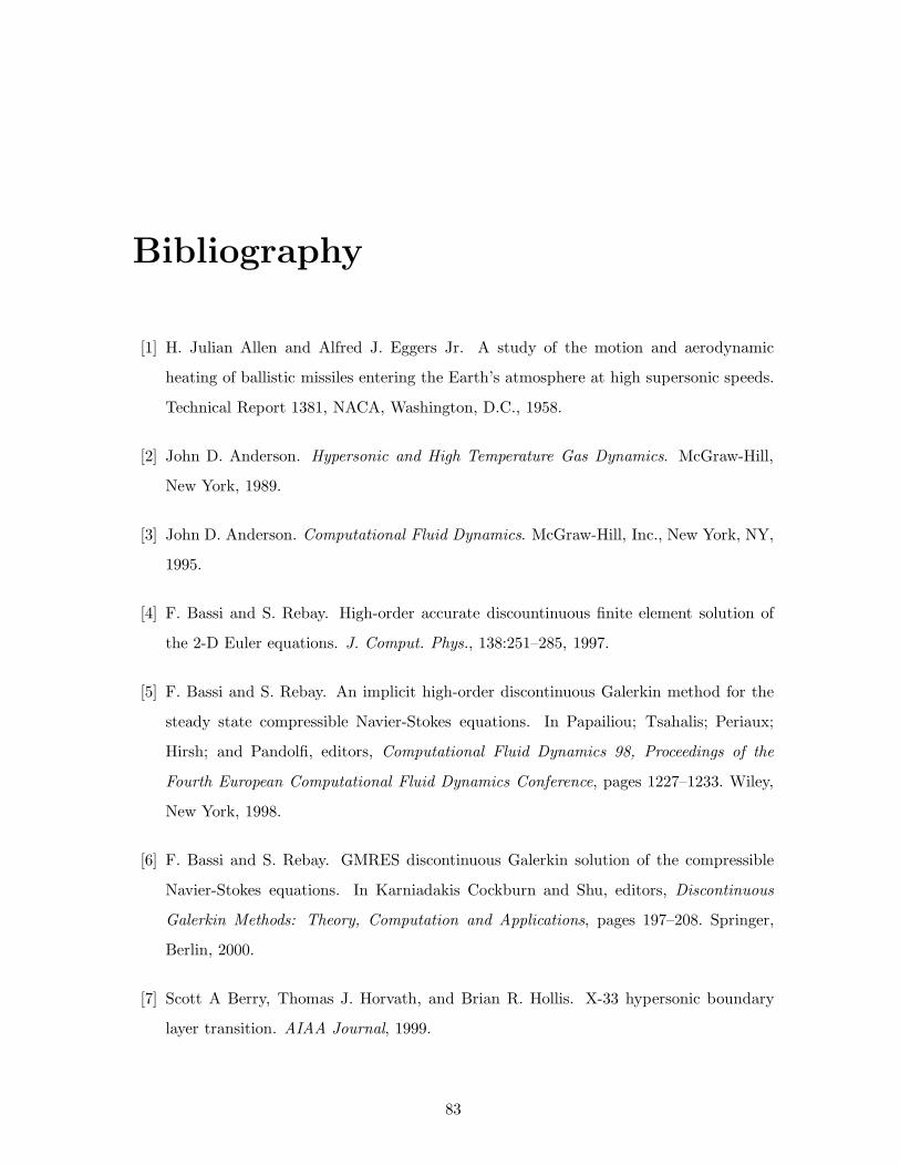
Bibliography

[1] H. Julian Allen and Alfred J. Eggers Jr. A study of the motion and aerodynamic

heating of ballistic missiles entering the Earth’s atmosphere at high supersonic speeds.

Technical Report 1381, NACA, Washington, D.C., 1958.

[2] John D. Anderson. Hypersonic and High Temperature Gas Dynamics. McGraw-Hill,

New York, 1989.

[3] John D. Anderson. Computational Fluid Dynamics. McGraw-Hill, Inc., New York, NY,

1995.

[4] F. Bassi and S. Rebay. High-order accurate discountinuous finite element solution of

the 2-D Euler equations. J. Comput. Phys., 138:251–285, 1997.

[5] F. Bassi and S. Rebay. An implicit high-order discontinuous Galerkin method for the

steady state compressible Navier-Stokes equations. In Papailiou; Tsahalis; Periaux;

Hirsh; and Pandolfi, editors, Computational Fluid Dynamics 98, Proceedings of the

Fourth European Computational Fluid Dynamics Conference, pages 1227–1233. Wiley,

New York, 1998.

[6] F. Bassi and S. Rebay. GMRES discontinuous Galerkin solution of the compressible

Navier-Stokes equations. In Karniadakis Cockburn and Shu, editors, Discontinuous

Galerkin Methods: Theory, Computation and Applications, pages 197–208. Springer,

Berlin, 2000.

[7] Scott A Berry, Thomas J. Horvath, and Brian R. Hollis. X-33 hypersonic boundary

layer transition. AIAA Journal, 1999.

83

[8] J. P. Boris and D. L. Book. Flux corrected transport I, SHASTA, a fluid transport

algorithm that works. Journal of Computational Physics, 11(1):38–69, 1973.

[9] Michael L. Brasher. Visualizing quadratic and cubic finite elements. Master’s thesis,

Massachusetts Institute of Technology, August 2004.

[10] P. G. Buning. Sources of error in the graphical analysis of CFD results. Journal of

Scientific Computing, 3(2):149–164, 1988.

[11] A. Burbeau, P. Sagaut, and Ch.-H. Bruneau. A problem-independent limiter for high-

order Runge-Kutta discontinuous Galerkin methods. Journal of Computational Physics,

169(1):111–150, 2001.

[12] Mark H. Carpenter and Jay H. Casper. Computational considerations for the simu-

lation of discontinuous flows. In V. Venkatakrishnan and et al., editors, Barriers and

Challenges in Computational Fluid Dynamics. Kluwer Academic Publishers, 1998.

[13] Jay Casper and Mark H. Carpenter. Computational considerations for the simulation

of shock-induced sound. SIAM Journal of Scientific Computing, 1998.

[14] M. J. Castro-Diaz, F. Hecht, B. Mohammadi, and O. Pironneau. Anisotropic un-

structured mesh adaptation for flow simulations. International Journal for Numerical

Methods in Fluids, 1997.

[15] Langley Research Center. Fully Unstructured Navier-Stokes (FUN3D) Product Man-

ual. National Aeronautics and Space Administration, Jan 2006. [Available online at

http://larc.nasa.gov/].

[16] B. Cockburn and C. W. Shu. The Runge-Kutta local projection p1-discontinuous

Galerkin method for scalar conservation laws. RAIRO Model Math. Anal. Numer.,

25:337–361, 1991.

[17] Vit Dolejsi, Miloslav Feistauer, and Christoph Schwab. On some aspects of the dis-

continuous Galerkin finite element method for conservation laws. Mathematics and

Computers in Simulation, 61(3):333–346, 2003.

84

[18] Peter A. Gnoffo et. al. Opportunities for breakthroughs in large-scale computational

simulation and design. Technical Report NASA/TM-2002-211747, Langley Research

Center, NASA, June 2002.

[19] Krzysztof J. Fidkowski. A high-order discontinuous Galerkin multigrid solver for aero-

dynamics applications. Master’s thesis, Massachusetts Institute of Technology, June

2004.

[20] Krzysztof J. Fidkowski and David L. Darmofal. Development of a higher-order solver

for aerodynamic applications. In 42nd AIAA Aerospace Sciences Meeting and Exhibit,

Reno, Nevada,. AIAA, January 2004. 2004-0436.

[21] Krzysztof J. Fidkowski, Todd A. Oliver, James Lu, and David L. Darmofal. p-multigrid

solution of high-order discontinuous Galerkin discretizations of the compressible Navier-

Stokes equations. Journal of Computational Physics, 207:92–113, 2005.

[22] Datta Gaitonde and J. S. Shang. Accuracy of flux-split algorithms in high-speed viscous

flows. AIAA Journal, 31(7), July 1993.

[23] P. L. George. Automatic Mesh Generation: Application to Finite Element Methods.

Wiley, Paris, 1991.

[24] Peter A. Gnoffo. Computational fluid dynamics technology for hypersonic applications.

AIAA/ICAS International Air and Space Symposium and Exposition, Dayton, Ohio,

July 2003. AIAA 2003-3259.

[25] Peter A. Gnoffo and F. McNeil Cheatwood. User’s Manual for the Langley Aerothermo-

dynamic Upwind Relaxation Algorithm (LAURA). Langley Research Center, National

Aeronautics and Space Administration, April 1996. NASA Technical Memorandum

4674.

[26] Peter A. Gnoffo and Jeffery A. White. Computational aerothermodynamics simulation

issues on unstructured grids. AIAA Journal, 2004.

[27] Henri Gouraud. Continuous shading of curved surfaces. IEEE Transactions on Com-

puters, 1971.

85

[28] Robert Haimes. Techniques for interactive and interrogative scientific volumetric visu-

alization. [Available online, http://raphael.mit.edu/visual3/visual3.html, Jan 2006].

[29] Robert Haimes. Visual3 User’s and Programmer’s Manual. Aerodynamics Compu-

tational Design Laboratory, Massachusetts Institute of Technology. [Available online,

http://raphael.mit.edu/visual3/visual3.html, Jan 2006].

[30] Robert Haimes and David Darmofal. Visualization in computational fluid dynamics: A

case study. In IEEE Visualization, 1991.

[31] Robert Haimes and Michael Giles. Visual3 – interactive unsteady unstructured 3D

visualization. In 29th AIAA Aerospace Sciences Meeting, Reno, NV, Jan. 7-10, 1991.

[32] Brian R. Hollis, Scott A Berry, and Thomas J. Horvath. X-33 turbulent aeroheating

measurements and predictions. AIAA Journal, 2002.

[33] Loyd S. Swenson Jr., James M. Grimwood, and Charles C. Alexander. This

New Ocean: A History of Project Mercury. National Aeronautics and

Space Administration, 1989. Special Publication-4201. [Available online at

http://www.hq.nasa.gov/office/pao/History/SP-4201/toc.htm, Jan 2006].

[34] L. Krivodonova, J. Xin, J.-F. Remacle, N. Chevaugeon, and J. E. Flaherty. Shock

detection and limiting with discontinuous Galerkin methods for hyperbolic conservation

laws. Applied Numerical Mathematics, 48(3):323–338, 2004.

[35] Aerospace Computational Design Laboratory. Project-X User’s Guide. Department of

Aeronautics and Astronautics, Massachusetts Institute of Technology, Nov 2005.

[36] Kelly R. Laflin, John C. Vassberg, Richard A. Wahls, Joseph H. Morrison, Olaf Broder-

sen, Mark Rakowitz, Edward N. Tinoco, and Jean-Luc Godard. Summary of data from

the Second AIAA CFD Drag Prediction Workshop. Technical Report 2004-0555, AIAA,

2004.

[37] S. K. Lele. Compact finite difference schemes with spectral-like resolution. J. Comput.

Phys., 103:16–42, 1992.

86

[38] Randall J. LeVeque. Numerical Methods for Conservation Laws. Birkhauser Verlag,

Boston, 1992.

[39] David W. Levy, Thomas Zickuhr, John Vassberg, Shreekant Agrawal, Richard A. Wahls,

Shahyar Pirzadeh, and Michael J. Hemsch. Data summary from the First AIAA Compu-

tational Fluid Dynamics Drag Prediction Workshop. Journal of Aircraft, 40(5):875–882,

2003.

[40] H. W. Liepmann and A. Roshko. Elements of Gas Dynamics. Dover Publications, Inc.,

Mineola, NY, 1985.

[41] G. Moretti and M. Abbett. A time dependent computational method for blunt body

flows. AIAA Journal, 1966.

[42] US Centennial of Flight Commission. Evolution of technology: Early reentry vehicles.

[Available online at http://www.centennialofflight.gov, Jan 2006].

[43] Todd A. Oliver. Multigrid solution for high-order discontinuous Galerkin discretizations

of the compressible Navier-Stokes equations. Master’s thesis, Massachusetts Institute

of Technology, August 2004.

[44] OpenGL. OpenGL. [Available online at http://www.opengl.org, Jan 2006].

[45] P.-O. Persson and J. Peraire. Sub-cell shock capturing for discontinuous Galerkin meth-

ods. In 44th AIAA Aerospace Sciences Meeting and Exhibit, Jan 2006.

[46] Jianxian Qiu and Chi-Wang Shu. Hermite WENO schemes and their application as lim-

iters for Runge-Kutta discontinuous Galerkin method: One-dimensional case. Journal

of Computational Physics, 193(1):115–135, 2004.

[47] Jianxian Qiu and Chi-Wang Shu. Hermite WENO schemes and their application as lim-

iters for Runge-Kutta discontinuous Galerkin method II: Two dimensional case. Com-

puters and Fluids, 34:642–663, 2005.

[48] James J. Quirk. A contribution to the great Riemann solver debate. In M. Yousuff Hus-

saini, Bram van Leer, and John Van Rosendale, editors, Upwind and High-Resolution

Schemes, pages 550–569. Springer, New York, 1997.

87

[49] R. Radespiel and R. C. Swanson. Personal communication. via Todd Oliver, Mas-

sachusetts Institute of Technology, Aerodynamics Computational Design Laboratory.

[50] L. Remaki, H. Beaugendre, and W. G. Habashi. ISOD – an anisotropic isovalue-oriented

diffusion artificial viscosity for the Euler and Navier-Stokes equations. Journal of Com-

putational Physics, (186):279–294, 2003.

[51] G. R. Richter. An optimal-order error estimate for the discontinuous Galerkin method.

Math. Comp., 50:75–88, 1988.

[52] Hermann Schlichting. Boundary Layer Theory. McGraw-Hill Book Company, Inc., New

York, seventh edition edition, 1979.

[53] Sung soo Kim, Chongam Kim, Oh-Hyun Rho, and Seung Kyu. Cures for the shock insta-

bility: Development of a shock-stable Roe scheme. Journal of Computational Physics,

2003.

[54] P. K. Sweby. High resolution schemes using flux limiters for hyperbolic conservation

laws. SIAM Journal on Numerical Analysis, 21(5):995–1011, 1984.

[55] Christoph W. Ueberhuber. Numerical Computation 2: Methods, Software, and Analysis.

Springer-Verlag, Berlin, Germany, 1997.

[56] Bram van Leer. Towards the ultimate conservative difference scheme. II - Monotonicity

and conservation combined in a second order scheme. Journal of Computational Physics,

14:361–370, 1974.

[57] Bram van Leer. Towards the ultimate conservative difference scheme. III - upstream-

centered finite-difference schemes for ideal compressible flow. Journal of Computational

Physics, 23:263–275, 1977.

[58] Bram van Leer. Towards the ultimate conservative difference scheme. V - a second-order

sequel to Godunov’s method (for ideal compressible flow). Journal of Computational

Physics, 32:101–136, 1979.

[59] John C. Vassberg, Mark A. DeHaan, and Tony J. Sclafani. Grid generation requirements

for accurate drag predictions based on OVERFLOW calculations. AIAA, 2003. 2003-

4124.

88

[60] Luiz Velho, Luiz Henrique de Figueirido, and Jonas Gomes. A unified approach for

hierarchical adaptive tesselation of surfaces. ACM Transacations on Graphics, 1999.

[61] David Anthony Venditti. Grid Adaptation for Functional Outputs of Compressible Flow

Simulations. PhD thesis, Massachusetts Institute of Technology, June 2002.

[62] V. Venkatakrishnan. Convergence to steady state solutions of the Euler equations on

unstructured grids with limiters. Journal of Computational Physics, 118:120–130, 1995.

[63] M. R. Visbal and D. V. Gaitonde. On the use of higher-order finite-difference schemes

of curvilinear and deforming meshes. Journal of Computational Physics, 181:155–185,

2002.

[64] J. von Neumann and R. D. Richtmyer. A method for the numerical calculation of

hydrodynamic shocks. Journal of Applied Physics, 21:232–237, 1950.

[65] Z. J. Wang. Spectral (finite) volume method for conservation laws on unstructured

grids. Basic formulation. J. Comput. Phys., 178:210–251, 2002.

[66] John F. Wendt. External hypersonic aerodynamics: State-of-the-art and future per-

spective. Advisory Group for Aerospace Research and Development, Working Group

18. North Atlantic Treaty Organization.

[67] David F. Wiley. Approximation and Visualization of Scientific Data Using Higher Order

Elements. PhD thesis, University of California, Davis, 2003.

[68] Nail K. Yamaleev and Mark H. Carpenter. On accuracy of adaptive grid methods for

captured shocks. Journal of Computational Physics, 2002.

[69] Y. Zhou, M. Garland, and R. Haber. Pixel-exact rendering of spacetime finite element

solutions. Proceedings of IEEE Visualization 2004, October 2004.

[70] D. W. Zingg, S. De Rango, M. Nemec, and T. H. Pulliam. Comparison of several spatial

discretizations for the Navier-Stokes equations. J. Comput. Phys., 160:683–704, 2000.

89

Hypersonic Heat Transfer and Anisotropic Visualization ... · Hypersonic Heat Transfer and...

Documents

Transcript of Hypersonic Heat Transfer and Anisotropic Visualization ... · Hypersonic Heat Transfer and...