\

AEDC TR-94-5

OCT 12 1994

"tftrr 12"1994 t~fi

TE

Hypersonic Flow-Field Measurelnents -Intrusive and Nonintrusive

R. K. Matthews and W. D. Williams Calspan Corporation! AEDC Operations

August 1994

Final Report for Period July 1992 ~ July 1993

Approved for public release; distribution is unlimited.

P'ROflERTY OF U.S. AIR rORet AtDC TEQllilCAl LIBRARY

ARNOLD ENGINEERING DEVELOPMENT CENTER ARNOLD AIR FOR'CE BASE, TENNESSEE

AIR FORCE MATERIEL COMMAND UNITED STATES AIR FORCE

NOTICES

When U. S. Government drawings, specifications, or other data are used for any purpose other than a definitely related Government procurement operation, the Government thereby incurs no responsibility nor any obligation whatsoever, and the fact that the Government may have formulated, furnished, or in any way supplied the said drawings, specifications, or other data, is not to be regarded by implication or otherwise, or in any manner licensing the holder or any other person or corporation, or conveying any rights or permission to manufacture, use, or sell any patented invention that may in any way be related thereto.

Qualified users may obtain copies of this report from the Defense Technical Information Center.

References to named commercial products in this report are not to be considered in any sense as an endorsement of the product by the United States Air Force or the Government.

This report has been reviewed by the Office of Public Affairs (PA) and is releasable to the National Technical Information Service (NTIS). At NTIS, it will be available to the general public, including foreign nations.

APPROVALSTA~ENT

This report has been reviewed and approved.

~/Y}~ DENNIS N. HUPRICH, Major, USAF Space and Missile Systems Test Division

Approved for publication:

FOR THE COMMANDER.

~~ CONRAD M. RITCHEY, Lt Col, USAF Space and Missile Systems Test Division

,

REPORT DOCUMENTATION PAGE Form Approved

OM8 No. 0704-0188

Public reporting burden for this collection of information is estimated to average 1 hour per response, including the time for reviewing instructions, searching eXisting data sources, gathering and maintaining the data needed, and completing and reviewing the collection of information. Send comments regarding this burden estimate or any other aspect of this collection of information, including suggestions for reducing this burden, to Washington Headquarters Services, Directorate for Information Operations and Reports. 1215 Jefferson Davis Highway. Suite 1204. Arlington. VA 22202-4302. and to the Office of Management and Budget. Paperwork Reduction PrO'ect (0704-0188i. Washinqton. DC 20503.

1. AGENCY USE ONLY (Leave blank) 12. REPORT DATE 13. REPORT TYPE AND DATES COVERED August 1994 Final ReDort for Julv 1992 - Julv 1993

4. TITLE AND SUBTITLE 5. FUNDING NUMBERS

Hypersonic Flow-Field Measurements - Intrusive and AF Job No. 0979 Nonintrusive

6. AUTHOR(S)

Matthews R. K. and Williams, W. D. Calspan Corporation/AEDC Operations

7. PERFORMING ORGANIZATION NAME(S) AND ADDRESS(ES) 8. PERFORMING ORGANIZATION (REPORT NUMBER)

Arnold Engineering Development Center/DOF Air Force Materiel Command

AE DC-TR-94-5

Arnold Air Force Base, TN 37389-4000

9. SPONSORING/MONITORING AGENCY NAMES(S) AND ADDRESS(ES) 10. SPONSORING/MONITORING AGENCY REPORT NUMBER

Arnold Engineering Development Center/DOF Air Force Materiel Command Arnold Air Force Base, TN 37389-4000

11. SUPPLEMENTARY NOTES

Available in Defense Technical Information Center (DTIC).

12a. DISTRIBUTION/AVAILABILITY STATEMENT 12b. DISTRIBUTION CODE

Approved for public release; distribution is unlimited.

13. ABSTRACT (Maximum 200 words)

Flow-field measurement techniques that require a probe or other device to be inserted into the flow are classified as "intrusive." In general, these intrusive techniques are currently viewed as inferior to the more popular nonintrusive techniques. However, it should be remembered that in general these intrusive techniques have evolved over several decades while the flow-field experience of nonintrusive techniques is relatively limited. Included in the intrusive classification are pitot tubes, total temperature probes, Mach/angularity probes, static pressure devices, and others. For many years nonintrusive diagnostics have also been under development to meet the demands of hypersonic testing. Today, a large number of nonintrusive techniques at various levels of maturity and complexity are available for application. These techniques provide measurement of species number density, rotational and vibrational temperatures, static pressure, flow velocity, and visualization of flow structure.

14. SUBJECT TERMS

flow-field measurement techniques nonintrusive techniques

intrusive techniques Reynolds number

17. SECURITY CLASSIFICATION 1 B. SECURITY CLASSIFICATION 19. SECURITY CLASSIFICATION OF REPORT OF THIS PAGE OF ABSTRACT UNCLASSIFIED UNCLASSIFIED UNCLASSIFIED

COMPUTER GENERATED

15. NUMBER OF PAGES 57

16. PRICE CODE

20. LIMITATION OF ABSTRACT

SAME AS REPORT

Standard Form 29B (Rev, 2-89) PreScribed by ANSI Std. Z39·18 298·102

AEDC-TR-94-5

FOREWORD

The hypersonic regime is the most severe of all flight regimes, and consequently demands smart utili­zation of ground testing and evaluation, flight testing, and computation/simulation methodologies. Because of this challenge, von Karman Institute (VKI) asked the Arnold Engineering Development Center (AEDC) to develop a comprehensive course to define the "Methodology of Hypersonic Testing." Seven American scientists and engineers, representing AEDC and the University of Tennessee Space Institute (UTSI), for­mulated this course from their background of over a century of combined experience in hypersonic testing.

The objective of the course was to present a comprehensive overview of the methods used in hyper­sonic testing and evaluation, and to explain the principles behind those test techniques. Topics covered include an introduction to hypersonic aerodynamics with descriptions of chemical and gas-dynamic phe­nomena associated with hypersonic flight; categories and application of various hypersonic ground test facilities; characterization of facility flow fields; measurement techniques (both intrusive and non-intru­sive); hypersonic propulsion test principles and facilities; computational techniques and their integration into test programs; ground-test-to-flight data correlation methods; and test program planning. The Lecture Series begins at the introductory level and progressively increases in depth, culminating in a focus on spe­cial test and evaluation issues in hypersonics such as boundary-layer transition, shock interactions, electro­magnetic wave testing, and propulsion integration test techniques.

To obtain a complete set of notes from this course write to:

Lecture Series Secretary von Karman Institute Charrissie de Waterloo, 72 B-16409 Rhode-Saint-Genese (Belgium)

The information contained in this report is a subset of the work described above.

1

AEDC-TR-94-5

CONTENTS

Page Hypersonic Flow Field Measurements - - - Instrusive. . . . . . . . . . . . . . . . . . . . . . . . . . . . . . . . . . . . . . .. 5

Hypersonic Flow Field Measurements - - - Noninstrusive .................................... 19

3

AEDC-TR-94-5

HYPERSONIC FLOW FIELD MEASUREMENTS --- INTRUSIVE

by R. K. MATTHEWS

Senior Staff Engineer Calspan Corporation/ AEDC Operations Arnold Engineering Development Center

ABSTRACT

Flow-field measurement techniques that require a probe or other device to be inserted into the flow are classified as "intrusive." In general, these intru­sive techniques are currently viewed as inferior to the more popular nonintrusive techniques that will be described in the next section. However, it should be remembered that in general these intrusive techniques have evolved over several decades while the flow-field experience of nonintrusive techniques is relatively limited. Included in the intrusive classification are pitot tubes, total temperature probes, Mach/angu­iarity probes, static pressure devices, and others. Within limits, each of these techniques can provide very useful data for the aerodynamicist.

NOMENCLATURE

d Diameter of pitot probe

L Model length

M Mach number

p Pressure

Pp Measured pitot pressure

P' 0 Pitot pressure downstream of a normal shock

Rp/Rw Pitot probe radial distance/model wall radius

RT/Rw Temperature probe radial distance/model wall radius

Re oo Free-stream unit Reynolds number

ReL Free-stream Reynolds number based on model length

Rex Reynolds number based on X

T Temperature

Tp Measured probe temperature

V Velocity

u Local velocity

5

X Axial distance

y Lateral distance

Z Vertical distance

Zp Probe height above model surface

IX Local flow angle

0 Boundary layer thickness

OT Boundary layer thickness based on' total temperature profile

e Density

II- Viscosity

Subscripts

e Condition at edge of boundary layer

o Stilling chamber condition

avg Average of all four cone pressures on MFA probe

00 Free-stream conditions

R Rake measurement

Superscripts

( - ) Root mean square value of fluctuating quantity

( - ) Mean value, average with respect to time

INTRODUCTION

An important element in the development and validation of a computational fluid dynamic (CFD) code for the design of a hypersonic vehicle is a data­base that characterizes both the local flow field and model surface properties. 1 In general, wind tunnel simulations of the aerothermodynamic flow field and surface properties using subscale models of hyper­sonic vehicles are very limited. For example, the maximum wind tunnel Reynolds number of subscale models is often too low relative to the flight Reynolds number, the flight real-gas effects cannot be ade­quately simulated in a ground test facility, and the

AEDC-TR-94-5

state of the boundary layer on the subscaled model often does not truly correspond to that of the flight vehicle. Therefore, the CFD code becomes the aero­dynamic designer's tool for predicting the perfor­mance of the flight vehicle, and the wind tunnel database becomes the basis for calibrating and validating many aspects of the CFD code.

eoo~oo (.,

STAGNATlON7 POINT

LAMINAR BL--.I

Figure 1. Typical missile configuration and flow field structure.

WHAT

.. FLOW-FIELD AND' BOUNDARY-LAYER MEASUREMENTS AT VARIOUS LOCATIONS ALONG THE TEST ARTICLE

WHY

III CODE SUBSTANTIATION III TO GAIN A BETTER UNDERSTANDING OF A SPECIFIC FLOW FIELD

HOW

III INTRUSIVE: PITOT PRESSURE, TOTAL TEMPERATURE, MACH/ANGULARITY PROBES TRAVERSED ACROSS FLOW FIELD WITH SURVEY MECHANISM

iii NON-INTRUSIVE: ELECTROIOPTICAL BEAMS TRAVERSED ACROSS FLOW FIELD (LDV, LlF)

Figure 2. Fundamentais of survey tests.

We have previously discussed techniques for the measurements of the forces and moments acting on the flight vehicle, and vehicle surface properties of pressure, temperature, and heating rates. Here, we will address techniques providing information on the local flowfield; that is, tlie flow properties between the model surface and bow shock (Fig. 1). The fundamentals of survey test in terms of the' 'What". "Why" and "How" are presented in Fig. 2. Flow­field measurement techniques that require a probe or other device to be inserted into the flow are classi­fied as "intrusive." The nonintrusive techniques which use electon/optical beams will be described in . the next section. The intrusive techniques are pitot tubes, total temperature probes, Mach/angularity probes, and others. Each of these techniques can provide very useful data for the aerodynamicist. However, it is extremely important that the experi­mental aerodynamicist work very closely with the

6

computational fluid dynamicist and that both parties clearly understand the limitation of their respective specialities.

Flow Field Measurements

The mechanisms used to obtain boundary-layer or flow-field data generally fall into one of three categories:

1. on-board 2. off-board or 3. rakes

A typical on-board probing system is shown in Fig. 3 and consists of a motor-driven probe support which provides motion of the probes through the flow field. This probe unit can be used to survey the flow field at the base of the model at any model roll angle and angle of attack. Multiple-probe installation can be used and the interchangeable probe head allows a variety of probe types to be used. Note that the base of the model provides an aerodynamic "windshield" for the motor; however, in hypersonic flows it is often necessary to also provide a water­cooled jacket.

Figure 3. On-board mounted probe.

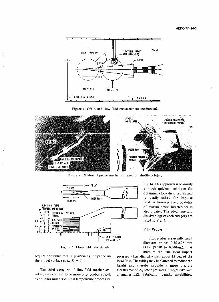
A typical off-board probing mechanism is shown in Fig. 4 and, as can be seen, this approach provides more flexibility, particularly for probes requiring significant travel along the model surface. Single or multiple probes can be traversed in two (X, Y) or three (X, Y, Z) directions as well as rotated (pitched) to generate data perpendicular to the model surfaces. An application of this approach (Fig. 5) provided valuable code validation data for the shuttle orbiter.

Typically, on-board and off-board probing mechanisms are limited to one to four probes and

48.5

., STA 55.923 STA 25.423

All DIMENSIONS IN INCHES

FlOW·FIElO SURVEY MECHANISM (X·Z)

MODEl

TUNNEl WALL

AEDC-TR-94-5

STA 0

Figure 4. Off-board flow-field measurement mechanism.

~;

.{

PROBING MECHANISM ..... -- INSTRUMENT PACKAGE

Figure 5. Off-board probe mechanism used on shuttle orbiter.

I' 200EG 30.0 (76 (m)--~--=::;:::::::==6~ "I o g ~ T"-.. ~ l.25-----1 "- COVER PLATE .

0.042·0.0. TOTAL TEMPERATURE PROBES

(3.18 (m)

\~.20 O.042.0.0.=(I=.0=7=m~m)~~ __ "::;;"_-.!L-T_--1J

0.' ~,,;, ;~~;:, '----'

0.4 g V :~:;~EGNED TO O.

o

Fig. 6). This approach is obviously a much quicker technique for obtaining a flow-field profile and is ideally suited for impulse facilities;"however, the probability of mutual probe interference is also greater. The advantage and disadvantage of each category are listed in Fig. 7.

Pitot Probes

MODEl SURFACE PRESSURE TAP Pitot probes are usually smaIi

diameter probes 0.25-0.76 mm O.D. (0.010 to 0.030-in.), that measure the true local impact

Figure 6. Flow-field rake details.

require particular care in positioning the probe on' the model surface (i.e., Z = 0).

The third category of flow-field mechanism, rakes, may contain 15 or more pitat probes as well as a similar number of total temperature probes (see

7

pressure when aligned within about 15 deg of the local flow. The tubing may be flattened to reduce the height and thereby provide a more discrete measurement (Le., probe pressures "integrated" over a smaller aZ). Fabrication details, capabilities,

AEDC-TR-94-5

TECHNIQUE

ON·BOARO

OFF·BOARD

RAKES

PROS

ACCESS TO PROBES, i.e., CAN CHANGE OUT PROBES

CONS

liMITED TO AFT PORTION OF MODEl

1,4 PROBES· LOW INTERFERENCE COMPLEX HARDWARE/COOliNG PROBABILITY ISSUES

ACCESS TO ANY MODEl STATION EACH SURVEY REQUIRES TIME TO POSITION PROBE ON MODEl

QUAlITY SURVEYS SURFACE AND TO TRAVERSE flOW FiElD RElATIVElY SLOWLY

HIGH PRODUCTIVITY

MAY REOUIRE TUNNEL SHUTDOWN TO ACCESS PRObES

POTENTIAL FOR PROBE INTERFERENCE

IDEAL FOR IMPLUSEIINTERMITTED FIXED NUMBER OF Y POSITIONS PER FACILITIES SURVEY

LIMITED MODEl STATIONS

limitations, and typical data are presented in Fig. 8. When attempting to survey a boundary layer, it is desirable that the ratio of the probe diameter to boundary-layer thickness be of the order of 0.2 or less (i.e., d/o :::; 0.2). Probe interference can occur when the probe bow shock impinges on the model surface, causing localized (very small) boundary-layer separa­tion as the probe gets to within one or two tip diameters of the model surface.

Total Temperature Probes

Figure 7. AEDC PROs and CONs of flow field survey

Total temperature probes (see Fig. 9) generally are either shielded or unshielded. The basic unshielded probe is simply a small ther­mocouple mounted in supporting tubing. The principle of operation is that the local flow will pass through the probe bow shock and stagnate at the thermocouple junction, raising the techniques.

GEOMETRY

(3.B mm) (3.B mm~1 0.032.in (O.B mm).DIAM

rO.15t~~~~ __ ~U!~_ -- ---'-- - ---"- -- ---

~= 0.012·IN. (0.3 mm) ·DIAM DRAWN (OR EXTRUDED) PITOT PROBE TIP

M", = B.O . Rex = 1.6 X 106

TO 4.0 X 106

O*-----------------~ o 1.0

TECHNIQUE It PROBE FABRICATION DEVElOPED 1969

CD CAPABILITIES

• WITH SURFACE STATIC PRESSURE, EXTRACT MACH NUMBER, VElOCITY AND BOUNDARY· LAYER PARAMETERS

It LIMITATIONS • VERY FRAGILE • SUBJECT TO INTERFERENCE ell PRESSURE STABILIZATION CRITICAL

4» COMMENTS • MINIMIZE PROBE INTERFERENCE • IMPROVE PRESSURE STABILIZATION

Figure 8. Pitot probe details.

8

temperature to the local total temperature. The assumption' is that conduction and radiation

losses can be accounted for by "calibration" in the freestream prior to the survey. The primary advantage of the unshielded probe is that it can be used within the boundary layer with less interference than the shielded probe. Shielded probes are clearly more susceptible to interference effects, but the intent of the "shield" is to minimize radiation losses. The shield quickly reaches a temperature approaching total temperature; therefore, the probe thermocouple "sees" a surrounding temperature that is relatively close to the local total temperature, thereby mini­mizing radiation losses. It is also important to consider the boundary layer growth within the shielding tube since fully merged flow will reduce the total temperature. These considerations are discussed in detail by Bontrager and Varner in Refs. 2 and 3, respectively.

Mach/Flow Angle Probes

The concept of using five-hole probes as flow­angularity measuring devices is based on the fact that the local Mach number and velocity direction can be uniqUely related to the circumferential variation in the surface pressure on a conical probe tip and the local pitot pressure. Generally, Mach flow angularity (MFA) probes are built to measure local stream pitot pressure and four circumferentially located static pressures ·(Fig. 10). With pressure measurements from these five orifices and suitable calibration constants, the local Mach number and flow direction of a supersonic/hypersonic flow field can be deter­mined. Calibration constants associated with Mach

• DEVElOPED It 1969 (HYPERSONIC FlOVl)

It CAPABILITIES .. DEFINE TOTAL TEMPERATURE PROFILES

• LIMITATIONS It FRAGILE It PITCH SENSITIVITY

It CONCERNS " INTERFERENCE PROBLEMS «I RAOIATION LOSSES

oS 0.2

~ d,

I

AEDC-TR-94-5

T JUNCTI N N p \0 fi O. 36 TC WIRE, 0

INSULATED SHEATIt~ .

I

F"""'""'"

L = 2d, 2d, l A

\ VENT HOLES, 2 'V I

10d,

SHIELDED TOTAL TEMPERATURE PROBE

Le - DISTANCE TO FULLY MERGED BOUNDARY LAYER INSIDE SHIELD TUBE

Pp = PITOT PRESSURE, PSIA

1.0 ~ T. = TRUE TOTAL TEMPERATURE, OR

1'; = 1,(9, LBF·SHlFT2 . ~ Av = TOTAL VENT AREA, FT2~ \.. 3.0 IN. .1

SHIELDED THERMOCOUPLE PROBE GEOMETRY

,.""" ,."

1

:= ;;rr:nf:tr- ~.6 1..---I..--I.....I....I...I...U..u...._l...-I......L..LI..IlJ.U._...L...LLLLLW

0.1

1->---- 3.0 IN~- U .. I UNSHIELDED THERMOCOUPLE PROBE GEOMETRY

10

L,IL = 0.0164 pN(L I', y'~) TYPICAL PROBE CALIBRATION CURVE

100

Figure 9. Total temperature probe details.

number and flow direction are determined from probe pressure data that are obtained during calibra­tion wind tunnel tests.

To fulfill a need to measure the local Mach number and velocity direction in a flow field or a boundary layer, miniature Mach flow angularity probes have been developed. Currently, two different machining techniques are used in the construction of these probes at AEDC. For probes with orifice dia­meters in the range of 0.2-0.3 mm (0.008-0.012 in.) and probe diameter of about 2.5 mm (0.10 in.), a precision jig bore (P JB) machine is used. Smaller probes with orifice diameters of 0.13-0.2 mIU (0.005-0.008) in. and probe diameters of about 1.75 mm (0.060 in.) are prepared with an Electrical Dis­charge Machine (EDM). The probes are generally machined to form a I5-deg half-angle cone. A comparison of P JB and EDM probes is shown in Fig. 10, which also shows some typical probe calibration data. The probes are currently calibrated in the Airflow Calibration Laboratory (ACL) of AEDC, which is a small test unit with IO-cm (4-in.) diam free­jet nozzles for Mach numbers from 1.75 to 6.0. This test unit has a 68-bar (l ,000 psia) air supply and can. provide airflows up to 4.54 Kgm/sec (10 Ibm/sec) and temperatures to 644°K (700°F). A photograph of a rake of probes mounted in the ACL is in Fig. 11 along with a close-up photograph of an EDM MFA probe. A description of MFA probe calibration and test procedures, including the equations used to

9

relate probe pressure measurements to local stream Mach number and flow direction is given in Ref. 4.

TYPICAL TEST RESULTS

Some results from flow-field tests of an early shuttle orbiter design in the AEDC Tunnel B at Mach 85 are given in Figs. 12 through 14. A rake of pitot and total temperature probes shown schematically in Fig. 12 was located at various stations along the wind­ward surface. Other measurements induded surface pressure and heat-transfer distributions. The rake

. flow-field profiles given in Fig. 12 demonstrate the use of the temperature data to .determine the edge of the boundary layer as the minimum value of Z where TR/To "" 1.0. As can be seen, the pitot pres­sure measurements could not be used for this pur­pose. Using the measured pitot pressure at Z = OT and the local surface pressure at the same station (see Fig. 13), the boundary-layer edge Mach number, Me, can be calculated. The edge Mach number can be us­ed in the calculation of other edge parameters such as temperature, Te, velocity, Jl.e, and Reynolds number, Re. The edge Mach number results are shown in Fig. 14 compared to Tangent Cone theory.

Flow Field Probing

Some results from tests utilizing the off-board probing technique on a conical reentry vehicle (RV) configuration in the AEDC Tunnel B at Mach 8 are given in Figs. 15 through 17. In this test an overhead probillg mechanism was used to survey the flow field

AEDC-TR-94-5

DEVElOPED

CAPABILITIES

1976 AEDC 1978 MINIATURIZATION

• MEASURE lOCAL PARAMETERS (MACH NO., flOW ANGLES, PRESSURES)

• MEASURE 3·DIMENSIONAl FLOW DIRECTION

LIMITATIONS . • FABRICATION TEDIOUS AND TlME·COUNSUMING

• ASYMMETRY OF TUBES AND ACCURACY OF CUTS (TUBE FACE ANGlES)VERY CRITICAL

• ALIGNMENT AND POSITIONING CRITICAL

COMMENTS • PERFORMANCE DIRECTlY DEPENDENT ON PRECISION OF FABRICATION

BOlAM (5 HOLES) TO INTERSECT ( DIAM

4 HOLES PERPENDICULAR TO TAPER

A*:~I~§im ~ --F---~.I

FABRICATION NOMINAL DIMENSIONS, mm (IN,) TECHNIQUE A B C 0 E

PRECISION JIG 1.0 0.2·0.3 0.38·0.51 0,64·0.76 2.54·3.0 BORE (P;8) (0.040) (0.008 - (0.015 - (0.025 - (0.10 -

0.012) 0.020) 0.030) 0.12)

ElECTRICAL 0.5 0.15·0.2 0.2·0.25 0.38·0.51 1.5-1.78 DISCHARGE (0.020) (0,006 - (0.008 - (0.015 - (0.060 -MACHINING 0.008) 0.010) 0.020) 0.070) (EDM)

0.10 .lP13 '" P3 - PI; PRESSURE DIFFERENTIAL ACROSS CONICAL PROBE

0,08

0.06

~I 0,04 ~ ;;; <:j

a:: <I

_,N

0.02

!!!:::.~

o....~

1.00

0,80

0.60 0.50

0.40

0,30

0.15

0,10 0.09 0.07

F 8.9 (0.35)

6.35 (0.25)

0.06 '--__ .J...._..L....-~--'-~_L_J 1.2 1.5 2,0 3,0 4,0 5.0 6.0 7.0 8,0 I 4 5 6 8 10

FREE·STREAM MACH NO. FREE·STREAM MACH NO,

Figure 10. Mach/flow angularity probe details.

~. a. Photograph of EDM probe. b. Calibration of Mach/flow angle probes.

Figure 11. Mach/flow angularity probe calibration.

10

" = 10 DEG, xll = 0.7, Re l = 9.0 X 106

1.0. O.B

;: 0.6 >. 0.4

0.2 5 o T

o 1.0 2.0 3.0 4.0 PR/p~

AEDC-TR-94-5

::ill§1 0.4 0.6 1.0 1.2

Figure 12. Typical rake pitot pressure and total-temperature profiles.

1.00 0.80

0.60

0.40

0.20

~ 0.10 0.08

0.06

0.04

0.02

0.01

:.\

~\

_l

~

o

SYM 01, DEG 0 10 0 20 0 30 Q 40 c, 50

TANGENT (ONE MODIFIED

NEWTONIAN

... ..... - - ....

"~ ['\

r'<l -~\

~ ~ ,0

M x = B I~ Re l = 9.0 x 106

0.2 0.4 0.6 0.8 1.0 x/l

Figure 13. Orbiter windward centerline pressure

distributions.

11

10.0

8.0

6.0

4.0

2.0

1.0

0.8

~

f0-r--

I / '/ fj

Y

o

-TANGENT (ONE

Moo = 8, Re l '" 9.0 x 1Q6

0.2 0.4 0.6 x/L

-/'

,/' /'

./ f""

1/ V

0.0 1.0

01, DfG SYM

10 0

20 0

30 c,

40 0

Figure 14. Orbiter windward centerline inviscid Mach

number distributions.

0.062·IN. (1.575mm) ·DIAM SINGLE· SHiElDED TEMPERATURE PROOE -~

0.455·IN. ': (1.56 mm)-

0.020·IN. (0.51 mm) ·DIAM ID 0.030·IN. (0.76 mm) ·DIAM 00

!'PlTOT TUBE F"-

D.5·IN. (12.7 mm)\\.

U5·IN. 1"-(44.45 mm)

I

Figure 15. Probe sketch.

AEDC-TR-94-5

100

0

8 -a: 10 :::::: tt& MODIFIED N WTONIAN 00

THEORV

UPSTREAM ::::.t-=:DOWNSTR~

1 I H1NG~ LINE I

16 12 o -4 -8 x, IN.

a. Surface pressure distribution for I-in. radius nose at ex = - 10 deg and flap deflection of 30 deg.

+X........., 1--~~~-36.50~~~~----l---l

:::=~I =~1~5.~O :§~I ~:!1_~A~DJUSTABLE HINGE

F---y""""C:=31,t===-

I -tlNTERCHANGEA8LE STEEL NOSES L CONFIG 2, l-IN.-NOSE-RADIUS

CONFIG 1, SHARP NOSE

b. Model sketch Figure 16. Surface pressure data and model sketch.

... -~ 3 ....

0

x=3 x =-3

BOW SHOCK X = 9 I

§ I

_ , .L, .. L, 'l' I 2

x = 3: 0 3 1 2

x = -3: 0 p/Po

a. Data for sharp nose cone

BOW SHOCK X = 9

x = 3

l15.2

12.7

10.16

7.62 3:

5.08

2.54

l15.2

12.7

10.16

7.62 3:

5.08

2.54

with the pitot pressure and total temperature probes shown in Fig. 15. A surface pressure distribution along with a sketch of the RV configuration are shown in Fig. 16 and pitot probe survey data for a sharp and blunt nose configuration are given in Fig. 17. The pitot pressure profiles include the boundary layer thickness, aT as determined from the total tem­perature profiles. For the sharp nose configuration, Fig. 17a, the 'Knee' in the pitot-pressure profile oc­curs at the same location as aT indicating a well­defined boundary layer with no interaction between the viscid and inviscid regions. The dominance of the nose is evident in the pitot profiles for the blunt nose configuration, Fig. 17b. These profiles do not show the characteristic 'Knee' delineating the viscid and inviscid regions. One can also note that the surveys at upstream locations extended through the bow shock.

~ = 9: 0 2 3 4

Another test illustrating flow-field probing is shown in Figs. 18 and 19. This test, also conducted in the AEDC Tunnel B, was an investigation of the influence of nose bluntness and incidence angle on the lees ide flow field of a 6-deg half-angle cone at Mach 6. The model, with a sharp nose, is shown in Fig. 18. The model was instrumented for surface pressure and heat-transfer measurements and had movable rakes of pitot pressure and total temperature probes. An overhead probing mechanism was also equipped with a pitot pressure and total temperature

12

x = 3: 0 1 2 4 x = -3: 0 2

p/Po

b. Data for l-in.-rad nose cone Figure 17. Flowfield distribution at ex = 0 and a = O.

probe (Fig. 18). A set of data from the flow-field probing is given in Fig. 19 in the form of contour plots (or isolines) of pitot-pressure and total­temperature ratios for a cone incidence angle of 12 deg. Presented in this manner, the data illustrate the complexity of the flow and the presence of a primary vortex and a secondary recirculation zone. The schematic inset in this figure shows the type of flow field encountered, which was also confirmed by sur­face pressure and heat-transfer distributions and by surface oil flow photographs. This type of detailed flow-field data for the leeside of a body at angle of attack illustrates the type of test needed to truly validate CFD codes.

6 OEG

1 l­I I 1

1===1 1

4.125 IN. (10.48 1m)

~J Figure 18. Typical probe and rake installation.

120

110

100

90

3.2

/] /'" 130

2.8 2.4 2.0 1.6 1.2 Rp/Rw

PilOT PRESSURE CONTOURS

0.8 0.4

AEDC-TR-94-5

Hot-Wire Anemometry Measurements

Considerations of the flow-field properties needed to characterize the flow around a hypersonic vehicle have emphasized the importance of studies of transition to turbulence in the associated boundary layers. Limitations in the analytical models of the flow have generally dictated reliance upon empirical foundations in formulating prediction methods. Important to a characterization of boundary-layer transition is information from the interior of the layer regarding the progression of small disturbances (flow fluctuat.ions) as a phenomenon related to the transition process. Hot-wire anemometry techniques are generally recognized as a principal method for

the measurement of flow fluctuation parameters.

Capabilities have been developed at AEDC for the fabrication of hot-wire anemometer pro.bes suitable for hypersonic flows (Fig. 20). The application of a hot-wire anemometer to the task of measuring fluctuating components of vaI;ious flow parameters is essentially the immersion of a very small heated wire into the flow and the observation of the heat-transfer phenomena which result. The basic principle of operation is that the heat capacity of the wire is so small that the local fluctuating heating can be sensed by the wire. A typical probe

!40 "­

OEG#'165 1]50 \

\

180 I

- VORTEX

RECIRCULATION ~~""--~

3.2 SEPARATION"" OIL FLOW ACCUMULATION LINES

L---~ SECTION NORMAL TO ~

170 180 1 6 160 \ \ I I .

150 \ \ 0.99

140 \ ' il.9?0.98

/ \ 0.94 0.90 1 2

. 0.98 q"OEG 130 " ~~~~:E 099

I , " 0:96 120, 0.8 Rp/Rw

.8 110_

-VT, 0.4 100-

90-

1.6 1.2 0.8 Rr/Rw

+ 0.4

TOTAL TEMPERATURE CONTOURS

0.4

Figure 19. Flow field surveys at x/L 0.75 and ex = 12 deg.

13

AEDC-TR-94-5

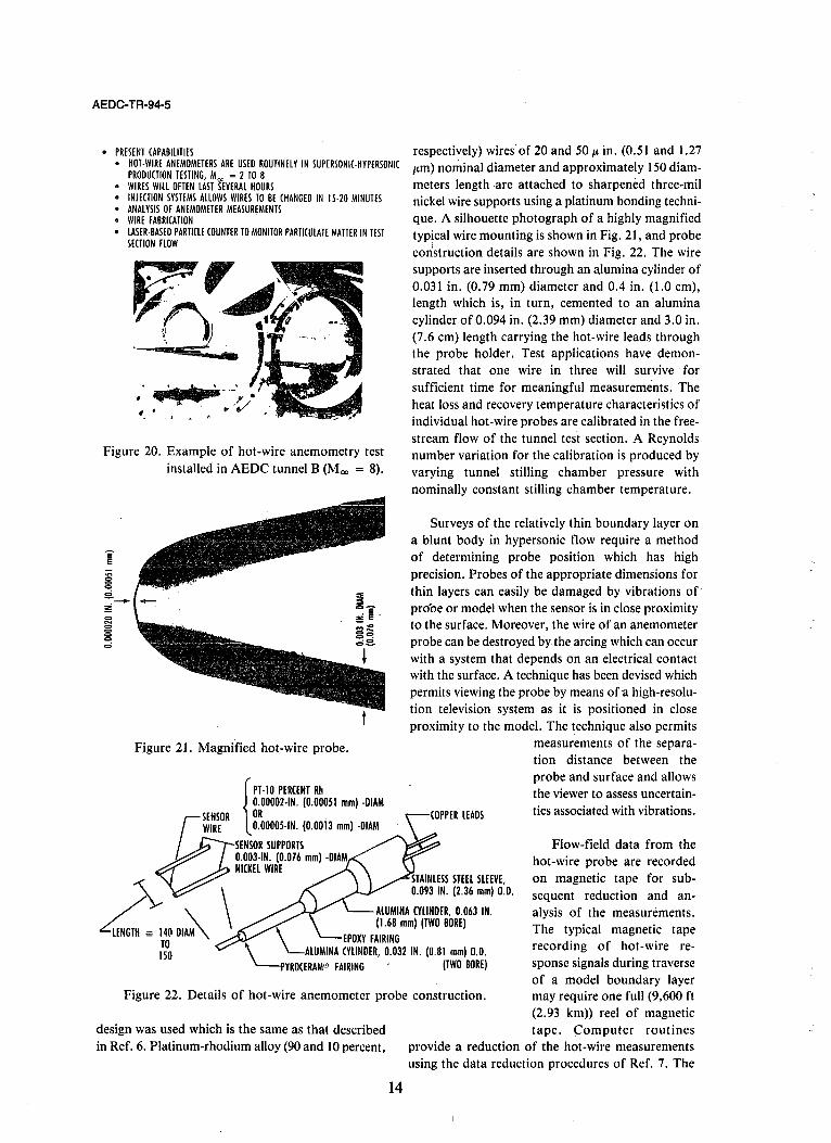
• PRESENT (APABILITIES • HOT·WIRE ANEMOMETERS ARE USED ROUTINElY IN SUPERSONI(·HYPERSONI(

PRODUCTION TESTING, Moo = 2 TO 8 • WIRES WILL OFTEN LAST SEVERAL HOURS • INJECTION SYSTEMS ALLOWS WIRES TO BE (HANGED IN 15·20 MINUTES • ANALYSIS OF ANEMOMETER MEASUREMENTS • WIRE FABRI(ATION • LASER·BASED PARTIClE COUNTER TO MONITOR PARTICULATE MATTER IN TEST

SECTION FLOW

••• . " ~~, .. / 4 • OV

Figure 20. Example of hot-wire anemometry test installed in AEDC tunnel B (Moo = 8).

Figure 21. Magnified hot-wire probe.

{

PT·\ 0 PERCENT Rh 0.00002-IN. (O.OOOS\ mm) -DIAM

SENSOR OR

O WIRE O.OOOOS-IN. (0.00\3 mm) -OIAM

~SENSOR SUPPORTS 0.003-IN. (0.076 mm) -OIAM NICKEL WIRE

respectively) wires of 20 and 50 p. in. (0.51 and 1.27 p.m) nominal diameter and approximately 150 diam­meters length ·are attached to sharpened three-mil nickel wire supports using a platinum bonding techni­que. A silhouette photograph of a highly magnified typical wire mounting is shown in Fig. 21, and probe construction details are shown in Fig. 22. The wire supports are inserted through an alumina cylinder of 0.031 in. (0.79 mm) diameter and 0.4 in. (1.0 cm), length which is, in turn, cemented to an alumina cylinder of 0.094 in. (2.39 mm) diameter and 3.0 in. (7.6 cm) length carrying the hot-wire leads through the probe holder. Test applications have demon­strated that one wire in three will survive for sufficient time for meaningful measurements. The heat loss and recovery temperature characteristics of individual hot-wire probes are calibrated in the free­stream flow of the tunnel test section. A Reynolds number variation for the calibration is produced by varying tunnel stilling chamber pressure with nominally constant stilling chamber temperature.

Surveys of the relatively thin boundary layer on a blunt body in hypersonic flow require a method of determining probe position which has high precision. Probes of the appropriate dimensions for thin layers can easily be damaged by vibrations of' pro'be or model when the sensor is in close proximity to the surface. Moreover, the wire of an anemometer probe can be destroyed by the arcing which can occur with a system that depends on an electrical contact with the surface. A technique has been devised which permits viewing the probe by means of-a high-resolu­tion television system as it is positioned in close proximity to the model. The technique also permits

STAINLESS STEEL SLEEVE, 0.093 IN. (2.36 mm) 0.0.

measurements of the separa­tion distance between the probe and surface and allows the viewer to assess uncertain-ties associated with vibrations.

L~"DI~ \ \ ALUMINA CYLINDER, 0.063 IN. '-- (\.68 mm) (TWO BORE)

Flow-field data from the hot-wire probe are recorded on magnetic tape for sub­sequent reduction and an­alysis of the measurements. The typical magnetic tape recording of hot-wire re­sponse signals during traverse of a model boundary layer may require one full (9,600 ft (2.93 km» reel of magnetic

TO ISO

\ EPOXY FAIRING \ LALUMINA CYLINDER, 0.032 IN. (0.8\ mm) 0.0.

'----i>YROCERAM® FAIRING' (TWO BORE)

Figure 22. Details of hot-wire anemometer probe construction.

design was used which is the same as that desqibed in Ref. 6. Platinum-rhodium alloy (90 and 10 percent,

14

tape. Computer routines provide a reduction of the hot-wire measurements using the data reduction procedures of Ref. 7. The

signals can be processed frequency-by-frequency or in broadband form. Quantitative hot-wire anemo­meter measurements obtained in discrete-point surveys of a sharp cone boundary layer, from Ref. 8, are shown in Fig. 23 reduced to the form of velocity and temperature fluctuations.

1.5 r,-----r------.--~

1.0

0.5

\

o~----~----~----~ o 0.1 0.2 0.3:

u/u OR TIT

AEDC-TR-94-5

Vapor-Screen Techniques

The vapor screen technique provides a means of visualizing and recording the flow pattern around a model in a plane perpendicular to the flow. The tech­nique requires that the wind tunnel be operated at conditions which permit water vapor condensation

to be present in the test section. At the AEDC this is accomplished by reducing the supply air temperature and/or bypassing the air driers.

Re", = 0.22 x 106 IN.-I

M =8 00

0.1 0.2 0.3

u/u OR TIT

Figure 23. Typicai variations of velocity and temperature fluctuations across the boundary layer of a sharp cone at zero angle of attack.

A thin sheet of light is projected along the plane of interest in the test section, usually perpendicular to the wind tunnel centerline or model axis. A schematic of the vapor screen apparatus is given in Fig. 24, and 'vapor­screen photographic com­posites of an elliptic body at Mach 3 in the AEDC Super-

FLOW VISUALIZATION METHODS

Two techniques in use for flow visualization that can be termed as intrusive are the vapor-screen and oil-flow techniques. 9

CYLINDRICAL LENS ~ CAMERA U LASER

a. Top view

~OW SHOCK BOUNDARY

MODEl -, '. VORTICE7 ;fj~~1)' "-,~~' . ,

\

_ CYLINDRICAL ' • .LENS

Gm:y:J LASER .

SHADOW FROM MODEL VAPOR SCREEN-"

!fij{' CAMERA

b. 3/4 view Figure 24. Schematic diagram 01 vapor screen

apparatus.

15

sonic Tunnel A are shown in Fig. 25. When there is no model in the test section, reflection and scattering of light by the water particles make this plane appear as a uniformly illuminated screen. When the model is inserted into this illuminated screen, the intensity of the reflected and scattered light varies, depending on the density of the water particles in the flow field around the model. In evaluating a vapor-screen photograph, one must consider the possible effects of the condensed flow condition in the test section on the phenomenon of interest. Ambiguous effects may be present because of variations in temperature in the flow field, causing evaporation in the heating areas and failure of the water particles to accelerate and decelerate at the same rate as the air because of their greater inertia. Qualitatively, however, the vapor screen flow visualization technique can be an extremely useful experimental tool, and the compo­site photographs of Fig. 25 present a very clear illustration of the lee-side vortex formation on the. elliptic body for angles of attack from 12 to 20 deg.

Oil Flow Technique

The oil-flow technique provides a means of visualizing and recording the flow pattern on the surface of a model and is particularly useful in locating regions of flow separation. Basically, the model is coated with a thin layer of oil which has be!!n pigmented to make the oil layer visible on the model surface. A low-viscosity silicon oil pigmented with

AEDC-TR-94-5

VORTI(ES

Figure 25. Vapor screen photograph composites of elliptic body, in tunnel A, at Mach 3.

Figure 26. Oil flow photograph of lifting body at

Mach 8.

titanium dioxide is often used. The model surface may also be painted to enhance the oil layer contrast on the surface. An oil-flow photograph of a lifting body configuration at Mach 8 in the AEDC Tunnel B is shown in Fig. 26, and a combined oil flow and shadow graph photograph of a blunt nose shape at Mach 10 in Tunnel C is given in Fig. 27.

16

FLOW , DIRECTION' )

/ /

Figure 27. Combined oil flow and shadowgraph photograph of blunt body, M = 10.

SUMMARY

The validation of CFD codes is a subject of increasing interest in the hypersonic community. Sur­face pressure and heat transfer distributions can provide a degrees of validation information however, flow-field data provide significantly more informa­tion and are perferred for code validation experi­ments. Flow-field measurement techniques have been developed that provide: pitot pressure, total tempera­ture, Mach flow angularity, hot-wire anemometry and flow visualization information. The hardware design and the test technique procedures have envolv­ed over many years and within limitations these techniques will continue to be the foundation for quality code validation experiments. However, it is extremely important that the experimental aero­dynamicist work very closely with the computational fluid dynamicist and that both parties clearly under­stlllld the limitations of their respective specialities.

REFERENCES

I. Matthews, R., Crosswy, F. and Sackleh, F. "Testing Capabilities at AEDC for Develop­ment of Hypersonic Vehicles," AIAA 91-5027, December 1991.

2. Bontrager, P. J. "Development of Thermo­couple-Type Total Temperature Probes in the Hypersonic Flow Regime," AEDC-TR-69-25 (AD-681489). January 1969.

3. Varner, Mike O. "Corrections to Single­Shielded Total Temperature Probes in Sub­sonic, Supersonic, and Hypersonic Flow," AEDC-TR-76-140 (AD-A032-725), November 1976.

4. Marquart, E. J. and Grubb, J. P. "Bow Shock Dynamics of a Forward-Facing Nose Cavity," AIAA-87-2709, October 1987.

5. Martindale, W. R., Matthews, R. K. and Trim­mer, L. L. Sverdrup Technology, Inc.! AEDC Division, Arnold AFS, TN. "Heat-Transfer and Flow-Field Tests of the North American Rockwell/General Dynamics Convair Space Shuttle Configurations." AEDC-TR-72-169 (AD-755354), January 1973.

6. Doughman E. L. "The Development of a Hot­Wire Anemometer for Hypersonic Turbulent

17

AEDC-TR-94-5

Flows." The Review of Scientific Instruments, Vol. 43, No.8, August 1972, pp. 1200-1202.

7. Morkovin, Mark V. "Fluctuations and Hot­Wire Anemometry in Compressible Flows." AGARDograph 24, November 1956.

8. Donaldson, J. C. "The Development of Hot­Wire Anemometer Test Capabilities for Moo =

6 and Moo = 8 Applications," AEDC­TR-76-88 (AD-A029570), September 1976.

9. Jones" J. H. and O'Hare, J. E. "Flow Visualization Photographs of a Yawed Tangent Ogive Cylinder at Mach Number 2," AEDC­TR-73-45 (AD-908178L), March 1973.

AEDC-TR-94-5

HYPERSONIC FLOW-FIELD MEASUREMENTS --- NONINTRUSIVE

by W. D. WILLIAMS

Section Head Calspan Corportationl AEDC Operations

Arnold Air Force Base, Tennessee

ABSTRACT

The area of hypersonic testing presents significant challenges to measurement science. Accurate and detailed data are required for test facility, propulsion system performance, and aerodynamic flow-field characterization. The measurements must be made in harsh environments with minimal flow perturba­tion and· with stringent requirements on uncertainty and spatial/temporal resolution and coverage. Furthermore, the complex chemical and thermo­dynamic environment requires understanding at the molecular level. Since the early 1960s, nonintrusive diagnostics have been under development to meet the demands of hypersonic testing. Today, a large. number of techniques at various levels of maturity and complexity are available for application. These techniques provide measurement of species number density, rotational and vibrational temperatures, static pressure, flow velocity, and visualization of flow structure. From these measurements, paJ'ame­ters such as Mach number, stagnation quantities, mass flow rate, turbulence level, equivalence ratio, combustion efficiency, degree of thermodynamic nonequilibrium, and degree of flow contamination can be determined.

This lecture reviews the techniques that are currently available, their basic principles, advantages, and disadvantages, and provides an assessment of the state of applicability of the techniques. A methodo­logy for diagnostics selection and application is presented, and problem areas with possible solutions are examined. Numerous references of both a general nature for review of the fundamentals required for a better understanding of the measurement principles and a specific nature to show the level of advance­ment of the techniques are provided.

19

c

d

E

FB

Fy

NOMENCLATURE

Cross-sectional area of laser beam, cm2

Cross-sectional area of laser beam observed, cm2

Electric field vector

Spontaneous emission rate, s - 1

Measured spontaneous emission rate, s-I

Speed of light in vacuum; mls or cmls

Calibration factors

Separation between electron beam­generated plasma columns, cm or m

Separation between LDV fringes, em

Molecular diameter of ith species, cm2 or m2

Particle diameter, cm2 or m2

Measured spacing between particles, cm or m

Energy; Joule, erg, or eV

Laser energy per pulse; Joule, erg, or eV

Electric field vector

Boltzmann fraction

Quantum yield

GM(TR, T v,A) Muntz G-factor for the electron beam fluorescence excitationl emission process

Overlap integral or convolution of spectral profiles, em or s

AEDC-TR-94-5

g(l')

h

IBG

k

L

Spectral profile

Voigt spectral profile

Planck's constant; Joule s or erg s

Electron beam current, amperes

Measured spectral intensity from flow with lamp shutter closed, w/cm2 nm

Measured spectral intensity from lamp through test cell with no flow, w/cm2 nm

Measured spectral intensity from test cell with no flow and with lamp shutter closed, w/cm2 nm

Measured spectral intensity from flow with lamp shutter open, w/cm2

nm

Incident and transmitted laser intensity, w / cm2

Intensity of radiation scattered from a single particle with polarization per­pendicular to and parallel to the scattering plane, or the intensity of the incident laser beams used in the CARS technique

Mie scattering coefficients for radiation with polarization perpendicular and parallel to the scattering plane, respectively

Laser intensity, w/cm2 or w/m2

Gladstone-Dale constant, m3/Kg

Wave vector of laser

Rayleigh scattering wave vector

Wave vectors for the CARS technique

Boltzmann's constant; J K-I or cm- I K-I

Integrated spectral absorption coef­ficient per molecule, cm or cm2 s - I

Wave vector

Reaction rate constants

Coherence length, m or cm

Transmission length of laser beam through flow, or separation distance between electron beam and Langmuir probe, m or cm

20

Lob

MW

m

m

n

n(p)

n(x)

A P(x)

p

Qc

Qph

Qpre

R

Rang/ext

S

SG

T

Texc

Length of scattering volume observed, cm or m

. Molecular weight; kg/mole or g/mole

Optical system magnification

Mass (kg or g)

Refractive index

Avogadro's number, mole-I

~umber density; m- 3 or cm- 3

Particle number density

Species x number density

Number density of gas species in near resonance conditions with an atomic line reversal species

Total gas number density, cm - 3

Power of transmitted and incident laser beam, w/cm2

Power of laser beam at focal volume, w/cm2

Electric polarization vector of a medium

Mie scattering depolarization ratio

Pressure; atm, bar, or Pa

Collisional quenching rate, s - I

Multiphotoionization rate, s - I

Predissociation rate, s - I

Detector quantum efficiency

Gas constant, J/kg mole K

The angular/extinction ratio which is fundamentally equal to the ratio of scattering cross section to extinction cross section

Detected signal or fringe shift

Specific gravity

Temperature, K

Excitation temperature, K

Rotational temperature, K

Vibrational temperature, K

Measurement volume, cm3

Flow velocity, m/s or cm/s

Photon absorption rate, s - I

x

z

,lA aL

,lE

&(1')

&A a, &A L

1)0

Qr, Qof

<Text

Separation distance between laser beams, cm

Particles size parameter

CARS interaction length, cm

Molecular polarizability of ith species

Film contrast parameter or natural energy level decay rate

Medium dielectric susceptibility of degree i, cm3/erg or m3IJouie

Optical phase difference

Spectral separation between laser line position and absorption line position, cm- I

Energy difference between ro-vibra­tional energy levels

Range of optical frequencies

Dopper shift in terms of frequency and wavenumber, respectively

time interval, s

Time interval between laser pulses, s

Energy differential between molecu­lar and atomic energy levels

FWHM of spectral profile

FWHM of laser line shape and absorption'line shape, cm- I

Optical system efficiency

Optical phase

Wavelength; m or cm

Wavenumber; m -lor cm- I

Rayleigh scattering angle

Frequency, s -I (Hz)

Mass density; kg/m3 or g/cm3; or depolarization factor

Mass density in test cell with flow and no flow or reference flow, respectively, kg/m) or g/cm3

Absorption cross section, m2 or cm2

Extinction cross section, m2 or cm2

Rayleigh scattering cross section, m2

or cm2

Total Mie scattering cross section, m2 or cm2

21

T

T(X)

Tc

Teb

Tm

00

w

AEDC-TR-94-5

Mie scattering cross section for radiation with polarization perpendi­cular to and parallel to the scattering plane, m2 or cm2

Fluorescence measurement interval, or interval between laser pulses, s

Equivalent lifetime of electron beam-excited species x, s

Temporal coherence, s

Time delay between electron beam pulses, s

Measurement interval, s

Collection optics solid angle, sr

Circular frequency, radians/s

BACKGROUND MATERIAL

In order to facilitate review of the available and emerging nonintrusive diagnostic techniques, some background material is required, The very nature of being nonintrusive implies the use of the electro­magnetic spectrum, and Fig, 1 provides useful infor­mation on units and conversion factors commonly used by f1Qw diagnosticians worldwide. Although the units of frequency and speed of light are straight­forward, the units of wavelength and energy are diverse and have evolved as a result of spectroscopic practices in different regions of the electromagnetic spectrum. Although the units of meter and centimeter are the standard, in practice the units of micrometer, nanometer, and even Angstrom are coinmonly used. The unit for wavenumber (Le., the number of waves per unit length) is practically always centimeter-I rather than meter - I. As a c(jutionary note, it is important to know whether wavelengths being used have been measured in vacuum or air. The units used for energy are most often Joule and erg, but, again, as a result of spectroscopic practices the units of electron volt and centimeter-I are frequently encountered.

As noted in Fig. 2, flow diagnosticians seldom use mass density in their work; instead, number density, the number of molecules or particles per unit volume, is normally used. This practice has evolved as a result of the close historical ties between physical chemistry, chemical physics, and statistical thermo­dynamics and with the use of spectroscopic techni­ques for measurement of gas/liquid properties. It is much easier to deal with chemical and physical rate equations when using number density rather than mass density. The conversion from number density to mass density for molecules requires the ratio of

AEDC-TR-94-5

BACKGROUND MATERIAL: UNITS/CONVERSIONS ( (SPUD OF LIGHT IN VACUUM)

I' (FREQUENCY) = h (WAVELENGTH MEASURED IN VACUUM) vo, - I' 1 h (WAVENUMBER) = - = -

( Avo,

I' : Hz (5-1), KHz, MHz, GHz .....

( : 2.99B x 108 mis, 2.998 x 1010 (m/s

A : m, (m, ~m, nm, A 1 A = 10-10 m; lnm = lOA; 1 A = 10-8 (m; l~m = 10+4 A

the results thereof are best understood through consideration of molecular energy level. diagrams such as shown in Fig. 3. Using a typical diatomic molecule in the ground electronic state, for example, the potential energy curve is that of an anhar­monic oscillator, and the discrete vibra­tional energy levels of the molecule are shown with typical spacing of approxi­mately 2,000 cm -1. A close examination of the vibr~tional energy levels reveals a fine structure, the rotational energy levels

-of the molecules with typical spacing of approximately 2 cm - 1. The dissociation enelgy of the molecule (i.e., the energy at which the molecule separates into its two atomic constituents), is also shown.

E (ENERGY) = h (PLANCK'S CONSTANT) I' = hc!Avo, (m) = 100h( ~ ((m-I)

E : Joule, erg, ev 1 eV = 1.6 x 10-19 J = 8,066 (m- I

h : 6.626 x 10-34 Joule.s, 6.626 x 10-27 erg.s

CAUTION

I' = ciAoir (WAVELENGTH MEASURED IN AIR) m (REFRACTIVE INDEX OF AIR)

~=_1_ m Aoir

Figure 1. Background material: units/conversions. When dealing with molecule/radiation interactions and the results thereof, it is common practice to use multiple level energy level diagrams and rate equations to describe and model the interaction processes. Figure 4 shows, for example, a four-level model of the processes that can occur as a result of absorption of radiation in level 1. Molecules are pumped to level 2 at a rate W12, and molecules in leve12 can spontaneously decay to energy level 3 while emitting radiation at the rate A23'

There are also two radiationless types of

NUMBER DENSITY, n == NUMBER OF MOLECULES/ATOMS/PARTIClES PER (m3 OR m3

FOR MOLECULES/ATOMS:

MASS DENSITY = Q (x) = nIx) MW(x) NA

WHERE MW (x) == MOLECULAR ATOMIC WT OF SPEClES x

NA == AVOGADRO'S NUMBER

FOR PARTICLES:

e(P) = nIp) SG(p) (1 gmicm3 OR 103 kg/m3)

WHERE SG(p) = SPECIFIC GRAVITY

Figure 2. Background material: number density. transitions from level 2 that can occur:' collisional quenching and predissocia­tion. In the collisional

,. §

>-' <.!> ffi ~ :;;i >= ~ .... 0 ....

·40,000

30,000

20,000

TYPICAL DIATOMIC MOLECULE, GROUND ELECTRONIC STATE

-----------I---+ ..... -_-VIBRATIONAL ENERGY

LEVELS, dE - 2,000 (m-I

o~~~~~~~~~~~. o 1.0 1.5 2.0 2.5 3.0 3.5 INTERNUCLEAR DISTANCE, A

-----DETAILED VIEW OF A VIBRATIONAL LEVEL

ROTATIONAL /""ENERGY LEVELS, =: dE - 2 (m-I

queI?:ching process, energy is transferred via collisions with all species of mole­cules to predominantly vib­rational modes. This pro-cess presents an obstacle to the use of fluorescence techniques for measure­ments of species density and temperature. The pre-

Figure 3. Background material: molecular energy levels. dissociation process occurs if level 2 has a potential

molecular weight to Avogadro's number, and for . particles, the use of the specific gravity of the particle material.is required.

The great majority of nonintru~ive diagnostic techniques involves the interaction of electromagnetic radiation with flow molecules. The interactions and

22

energy curve which over­laps a repulsive electronic state of the same molecule. In this case many molecules in level 2 dissociate into atomic components carrying excess translational energy. The predissociative process serves to counter the effects of the collisional quenching process, because the effective lifetime of level 2 is reduced to such a degree that very few collisions between level

2 molecules and the other molecules can occur. Also shown in Fig. 4 is a multiphotoionization process which can also serve to decrease the effective lifetime

----.-=====,---- 4 (IONIC) MULTIPHOTOIONIZATION RATE = Oph' \-1

AEDC-TR-94-5

of level 2. If the incident pumping radiation has a high power density, mUltiple photons may act together (i.e. combined energy) to raise molecules from level 2 to ionic levels.

__ ~~-L ______ ~ ______ ~_2

I SPONTANEOUS i't. EMITTED ! COLLISIONAL QUENCHING J. EMISSION I "PHOTON(S) (RADIATION LESS) RATE,

PREDISSOCIATION RATE An \-1 D" \-1

,/' hv, INCIDENT

PHOTON(S)

(RADIATION LESS) " 3 RATE = Dp,,' \-1

ABSORPTION RATE = W12, \-1

ELECTRONIC ENERGY LEVELS

(STATIONARY STATES)

Figure 4. Background material: molecular transitions (real),

While the molecular levels shown in Fig. 4 are all real (i.e., stationary states), transi­tions can also occur that involve what is termed virtual levels as shown in Fig. 5. Consider incident radiation that is not resonant with a transition between real levels. The electric field can distort the electron cloud and create a virtual energy level that can be described as a sum over all stationary states of the molecule. The life­time of the interaction is on the order of 10- 12 - 10- 14 sec, and the incident photons involved in the interaction are scattered. If the incident radiation is nearly resonant with a transition between real levels, the photons are termed resonantly scattered.

DURATION OF SCATTERING PROCESS - 10-12 -10-14 \ ______________ 2 (VIRTUAL)

2 (REAL) 'RESONANTLY SCATTERED

PHOTONS ---1 (VIRTUAL)

- -~-'-'-==--'---'-- 1 (REAL) ,/ ELECTRONIC ENERGY

/ LEVELS hv, INCIDENT

PHOTON(S}

Figure 5. Background material: molecular transitions (virtual).

NATURAL BROADENING E

E(O)~ E = E(o)e-~t ~-

e _ If" TIME, I ".

In spite of the perfectly discrete levels implied by the previous diagrams, there are always broadening mechanisms associated with energy levels and transi-. tions. These transition widths are caused by several broadening mechanisms, and three of the most im­portant are illustrated in Fig. 6 for an emission transition from level 2 to level 1. The natural broa­dening process is the result of the finite lifetime of level 2 with no collisional or predissociative processes involved. The exponential decay of level 2 yields a

(A LORENTZIAN PROfilE)

DOPPLER BROADENING _V, 0<{ /""\../\.f"' 0 '1JlM

RADIATING MOLECULE

v = v. (I ± 1)

COLLISION BROADENING RADIATING MOLECULE

I I O.MtVWV1

I I

COLLISIONS INTERRUPT THE RADIATION PROCESS

(A GAUSSIAN PROFILE)

(A LORENTZIAN PROFILE)

-4 (1'n2) (v - vi/liv~ go (v) = e

livo = 2 (1'n2)112 ~ Ct

Ct = (2!T fl2 = (!~fl2

~ = ~ = O~D = 7.16 x 10-7 ( T )112 v. Ao A. /loW"

liv, = C p(olm) (T"rfT)O

Figure 6. Background material: transition widths.

23

AEDC-TR-94-5

Lorentzian frequency profile, gN(V), with a full width at half-maximum (FWHM) of oVN = )'/27r. The Doppler broadening process is the result of the movement of the molecule during the emission process. The frequency of the emission is shifted upward or downward depending on whether the molecule is moving toward or away from the observer. The process yields a Gaussian frequency profile, go(v), with a FWHM of 01'0 = 1'0 (7.16 X

10 -7) (T /MW) 112 where T is the temperature and MW is the molecular weight of the emitting species. Collision (or pressure) broadening results from the emission process being interrupted by'a collision of a level 2 molecule with other molecules. The collision broadening process also produces a Lorentzian frequency profile with a FWHM of aVe = Cp(T ref/T)a, where p is the total static pressure, T is the static temperature, T ref is a reference temperature, and C and IX are experimentally determined constants.

INTERFERENCE:

the source spectral profile with the molecular transition profile, and this is the overlap integral shown in Fig. 8. The source and transition profiles are independently normalized to unity through the integral over all frequencies.

• MUST FREQUENTLY CONVOlVE RADIATION SOURCE PROFILES (LASERS, LAMPS) WITH GAS SPECIES TRANSITION PROFILES

• THE CONVOLUTION IS CALLED THE OVERLAP INTEGRAL

f gyS (v - vSi)dv = 1. f gyt{v - vti) dv = I

-00

Figure 8. Background material: overlap integral.

For most of the hypersonic testing regime, the Doppler broadening mechanism is dominant. Nevertheless, a combination of broadening mecha­nisms is often required to describe emission/absorption/scattering pro­cesses with high accuracy. As shown in Fig. 7, Lorentzian widths add linearly and Gaussian widths combine by the sum of the squares. The convolution of a Gaussian with a Lorentzian profile is called a Voigt profile. Use of the Voigt profile is common in computa­tional models of emission/absorp­tion/scattering processes. Because all radiation sources also have finite frequency profiles, the modeling of the interaction of the radiation with molecules requires the convolution of

CONSIDER TWO PLANE WAVES ~I SCREEN

E, .. A,e1(k,., -wt+~,) 0 ____ 1. _____ P{r)

E2 .. A~'(k 2" - wt + ~2) _ FOR 4>, -4>2 = A CONSTANT, E 2 A STATIONARY FRINGE

_ _ PATTERN IS OBSERVED Ip on IA,1 2 + IA212 + 2A, • A2 101 ,<l

- - - -,<l 10k, • r - k2 • r + 4>, -4>2

COHERENCE:

REAL LIGHT SOURCES HAVE A RANGE OF FREQUENCIES, ,<lvs

THE LENGTH OF TIME OVER WHICH ONE MAY ACCURATELY PREDICT THE PHASE AT A GIVEN POINT IS A MEASURE OF TEMPORAL COHERENCE.

SPATIAL COHERENCE IS A MEASURE OF THE PHASE CORRELATION FROM DIFFERENT REGIONS OF A SOURCE. ..

Figure 9. Background material: interference/coherence.

IN MOST CASES A COMBINATION OF BROADENING MECHANISMS IS IN EFFECT

LORENTlIANS ADO LINEARLY: OVt = oVll + OVt2 + , ..

GAUSSIANS COMBINE BY THE RULE: {oVD)2 = {OVDI)2 + {ovD2)2 + ...

THE CONVOLUTION OF A GAUSSIAN WITH A LORENTZIAN PROFilE IS A VOIGT PROFILE:

'" gy (x) = CONST. I

x = 2v'en2 v - Vo oVD

e-y2 --=---dy {x-y)2 + 02

r Qy (x) dx = I , CONST = ~ ~ . b1D 1/'3/2

Figure 7. Background material: transition widths.

24

Two important aspects of electromagnetic radia­tion are interference and coherence. Considering two plane waves incident on a screen, a stationary fringe pattern (created by constructive and destructive inter­ference) with the intensity distribution given in Fig. 9 is observed if the phase difference between the two waves is a constant. The two plane waves of Fig. 9 are said to be mutually coherent. As noted earlier, all real radiation sources have a range of frequencies, Ill's. Temporal coherence is thl! length of time over which the phase of a wave may be accurately pre­dicted at a given point. The coherence time is Te = 11 Ill's and the corresponding coherence length is fe =

CTe• Spatial coherence is a measure of the phase correlation from different regions of a radiation source. A high degree of spatial coherence can be

achieved even with a broadband spectral source through the use of small apertures, but the penalty paid is very low spectral radiance. This is the advan­tage of using laser systems, because both high temporal and spatial coherence can be achieved with­out sacrificing power output.

Indeed, modern laser systems can create extre­mely high power densities, e.g., 109 - 1012 w/cm2,

and associated with these power densities are high electric field strengths which readily introduce non­linear optical phenomena. Expressing the electric polarization of a medium as a function of an applied electric field strength and dielectric susceptibility as in Fig. 10, permits an introduction to nonlinear optics. The first or linear term involves the familiar terms of dielectric constant and refractive index. For gases and liquids the second term is zero, but in crystals it is responsible for frequency doubling and mixing phenomena. The third term is responsible for phenomena such as frequency tripling, two-photon abso'rption, and coherent Raman effects.

References 1-7 provide excellent background material for in-depth reading in spectroscopy, inter­ferometry, optics, and lasers.

• INELASTIC

o ELASTIC

• REFRACTIVE

o HYBRID

AEDC-TR-94-5

Figure 11. Technique categorization: interaction process.

• L1NE·OF-SIGHT(LOS)

~ FLOW

• LOCAL

~ FLOW

I EXCITATION

SOURCE

RECEIVER/DETECTOR

ACTIVE

~EX(lTATION

SOURCE

P

! "CE"'"DElE"" PASSIVE

6~ RECEIVER ------0 DETECTOR

Figure 12. Technique categorization: observation method.

• MODERN LASER SYSTEMS CONCENTRATE ENERGY IN SPACE AND TIME; EXTREMELY HIGH POWER DENSITIES ARE POSSIBLE, 109 - 1012 WATTS/(M2

• AT 1010 WATTS/(M2, 1£1- 2 x 106 VOLTS/CM .

THE ELECTRI( POLARIZATION OF A MEDIUM (AN BE EXPRESSED AS:

p =,(1). E +\(2), EE + :P),EEE + ...... .

observation methods (Fig. 12), there are line-of­sight (LOS) and local categories. LOS methods include active and passive observation techni­ques. LOS active observation involves monitor­ing the transmission of electromagnetic radiation across the flow field while passive sampling involves monitoring the electromagnetic radia­tion generated from the flow field itself. For local methods a radiation source is transmitted across the flow-field region of interest, and at some point along the radiation path scattered/emitted radiation is sampled to provide a measurement at that point.

WHERE £ IS THE APPLIED ELECTRI( FIELD, x(i) IS THE DIELECTRI( SUSCEPTIBILITY

\(1) :::!>DIELECTRI( CONSTANT, REFRACTIVE INDEX

\(2) ::::> 0 IN GASES AND LIQUIDS, BUT RESPONSIBLE FOR FREOUEN(Y DOUBLING AND PARMETRIC MIXING IN CRYSTALS

\(3) :::!> FREQUEN(Y TRIPLING, TWO·PHOTON ABSORPTION, COHERENT RAMAN EFFECTS, ETL

Figure 10. Background material: non-linear optics.

TECHNIQUES

Categorization

The many nonintrusive diagnostic techniques available can be categorized in terms of the electro­magnetic wave/molecule (or particle) interaction process or the observation method. The interaction categories (Fig. 11) are elastic (no energy exchange),

\V\elastic (energy exchange), refractive (phase modula­tion caused by refractive index variations), or hybrid (Le., combinations of the other categories). As for

25

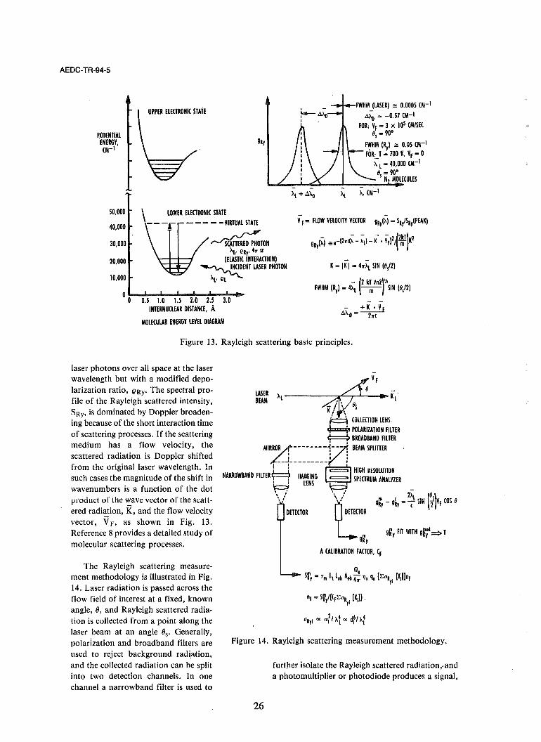
Rayleigh Scattering

The Rayleigh scattering technique is an elastic. local method for measurement of total species number density (nT), static temperature (T), and a flow velocity component (VF). In addition, the technique can effectively provide flow visualization. As illustrated in Fig. 13, incident laser radiation with wavelength, AL, and depolarization ratio, QL,

induces transitions from vibrational levels to a virtual state with a subsequent transition to the original vibrational levels and the scattering of the incident

AEDC-TA-94-5

I'OTENTIAL ENERGY, CM-I

50,000

UPPER ELECTRONIC .STATE

LOWER ELECTRONIC STATE

...... FWHM (LASER) :: 0.0005 CM-I

t.>:;' '" -0.57 CM-I FOR: VF = 3 x lOS CM/SEC

81 = 900

F~HM (Ry) :: 0.05 CM-I FOR: T = 700 K, VF = 0 ~ l = 40,000 CM-I 8 = 900

1 N MOLECULES

40,000 - - - - ~ VIRTUAL STATE V f '" FLOW VELOCITY VECTOR 9Ry(A) = VSRy(PEAK)

30,000 ~TON - - - - (2kT) 9RY(~) ::e-[2.-cIA - Al) - K • YF121 m K2

hl' eRY' 4 .. SI

(ELASTIC INTERACTION) 20,000 ~ENT LASER PHOTON K = IK I = 4 .. \ SIN (8/2)

10,000 hl' III - (2 kT en2)'"

00 FWHM (1Iy) = 4Al -m - SIN (8/2)

0.5 1.0 1.5 2.0 2.5 3.0 INTERNUCLEAR DISTANCE, A - ~

t.ho = 2 .. ( MOLECULAR ENERGY LEVEL DIAGRAM

Figure 13. Rayleigh scattering basic principles.

laser photons over all space at the laser wavelength but with a modified depo­larization ratio, QRy' The spectral pro­file of the Rayleigh scattered intensity, SRy, is dominated by Doppler broaden­ing because of the short interaction time of scattering processes. If the scattering medium has a flow velocity, the scattered radiation is Doppler shifted from the original laser wavelength. In such cases the magnitude of the shift in wavenumbers is a function of the dot product of the wave vector of the scatt­ered radiation, K, and the flow velocity vector, V F, as shown in Fig. 13. Reference 8 provides a detailed study of molecular scattering processes.

The Rayleigh scattering measure­ment methodology is illustrated in Fig. 14. Laser radiation is passed across the flow field of interest at a fixed, known angle, 0, and Rayleigh scattered radia­tion is collected from a point along the laser beam at an angle Os. Generally, polarization and broadband filters are used to reject background radilltion, and the collected radiation can be split into two detection channels. In one channel a narrowband filter is used to

LASER }.l-----"2"''''--I--'---tlO>- K l BEAM ••

v.i '. b (OLLEUION LENS 4mmmia POLARIZATION FILTER ¢::::::=:J BROADBAND FILTER

MIRZOR --------~---: BEAM SPLITTER . , . , " I "

__ ~_________ t

Ll HIGH RESOLUTION NARROWBAND FILTER'r-j' IMAGING SPECTRUM ANALYZER

I I LENS q , . '\ "

DETECTOR

Figure 14. Rayleigh scattering measurement methodology.

26

further isolate the Rayleigh scattered radiation,. and a photomultiplier or photo diode produces a signal,

Slry, which is a linear function of the total species number density and the sum of the scattering cross section and species mole fractions for all flow species. If there are no chemical reactions and the flow species and mole fractions are known, then the total species number density of the flow can be determined through a calibration process. The other detector channel can contain a high-resolu­tion spectrum analyzer such as a Fabry-Perot interferometer which can produce a measurement of the Rayleigh scattering spectral profile, glry ' A computer-generated Rayleigh scattering profile can be generated using the formulation in Fig. l3 and fit to glry through variation of the value of static temperature. The best fit yields a determination of static temperature. Furthermore, the measured separation between glry and a spectral profile measured at no-flow calibration conditions, gky, yields a determination of the velocity component along the path of the laser beam using the Doppler shift relations given in Fig. 13. Note that the Rayleigh scattering cross section, URyj, is inversely proportional to the fourth power of the laser wavelength; therefore, operation in the ultraviolet (UY) spectral region can produce greatly enhanced signals. Another key point is that the scattering cross sections are proportional to the square of the molecular species polarizability, af, which can also be expressed as proportional to the sixth power of the equivalent diameter, dr, of the scattering molecular species. This indicates that any particles in the observation volume can drastically affect the Rayleigh scattered signal.

The advantages and disadvantages of the Rayleigh scattering technique are tabulated in Fig. 15. Although the technique is relatively simple and low cost, it does require considerable optical design and careful installation to reduce background radia­tion. For a typical test cell arrangement, the back­ground radiation can be reduced to approximately 10 - 5 of the Rayleigh scattering signal with static, atmospheric conditions in the test cell. Certainly high spatial and temporal resolution are possible, but high­power cw or high-energy pulsed lasers are required. Determinations of total number density and tempera­ture are possible, but the flow must be nonreacting and particle-free. Furthermore, velocity determina­tion depends on the reliability of particles following the flow. When the conditions of nonreaction and no particles exist, visualization of density, tempera­ture, and velocity is possible, but requires the use of laser sheet-forming optics and array detector systems. Rayleigh scattering can be an excellent detector of

AEDC-TR-94-5

molecular nucleation; unfortunately, there is no method to deconvolve dependence on nucleate size and number density for nonmonodisperse distri­butions.

ADVANTAGES

RELATIVELY SIMPLE AND LOW COST

DISADVANTAGES

• REQUIRES GREAT CARE IN DESIGN AND PLACEMENT OF OPTICAL BAFFLES, APER· TURES, VIEWING DUMP, AND LASER BEAM RECEIVER AND IN SELECTION OF LASER TO REDUCE BACKGROUND RADIA· TlON AT LASER WAVELENGTH

• HIGH SPATIAL AND TEMPORAL RESOLUTION POSSIBLE

REOUIRES HIGH POWER CW OR HIGH ENERGY PULSED LASERS

• DETERMINE nT REQUIRES NON·REACTlNG, PARTICLE· FREE FLOW OF KNOWN COMPOSITION

27

DETERMINE VF

DETERMINE T '"

FLOW VISUALIZATION OF nT' vF' T '" IMULTANEOUSlY

DETECTION OF MOLECULAR NUCLEATION

ANY PARTICLES PRESENT MUST FOLLOW THE FLOW

MUST BE PARTICLE FREE, Nml·REACTING FLOW OF KNOWN COMPOSITION

REQUIRES SHEET FORMING OPTICS FOR LASER BEAM AND ARRAY DETECTOR SYSTEMS

UNABLE TO SEPARATE DEPENDENCY ON NUClEATE SIZE AND NUMBER DENSITY: WAL) < 0.1

l'i~lIn~ 15. Rayleigh scattering measurements.

NUMEROUS SMALL FACILITY APPLICATIONS: - HOMOGENEOUS/HETEROGENEOUS CONDENSATION IN UNDEREXPANDED NOZZlE

FLOW INTO HIGH VACUUM - MACH 2·3 LABORATORY WIND TUNNEL DIAGNOSTICS - GAS CONCENTRATION IN TURBULENT JETS - 20 VElOCITY AND TEMPERATURE IN LOW SPEED AIR JET

A FEW LARGE fACIlITY SUCCESSES: - HYPERSONIC HELIUM FLOW - CONDENSATION EFFECTS IN A HYPERSONIC WIND TUNNEl

• MOST LARGE FACILITY APPLICATIONS HAVE FAILED BECAUSE OF PARTICLES AND/OR HIGH BACKGROUND AT LASER WAVELENGTH e.g. BOEING 30·INCH HYPERSONIC SHOCK TUNNEl '

A STUDY HAS SHOWN FEASIBIlITY FOR A SPACE SHUTTLE APPLICATION TO MEASURE ATMOSPHERIC DENSITY DURING ENTRY; PLANS FOR APPLICATION IN AEOC 1M· PULSE FACILITY FOR He DRIVER GAS DETECTION

PACING TECHNOLOGIES: - flOW ClEANLINESS - HIGH REPETITION RATE PULSED LASERS (IN UV REGION, ESPECIAllY) - HIGH FRAME RATE ARRAY DETECTORS

Figure 16. Rayleigh scattering: state of applicability.

There have been numerous, successful small facility applications, e.g., those shown in Fig. 16, with measurements in underexpanded nozzle flows,9, to laboratory wind tunnels,lI, 12, 13 and low-speed jets. 14, 15 There have been only a few large facility successes, for example a hypersonic helium flow, 16

a hypersonic wind tunnel. 17 and a H2/02 thruster plume in an altitude space chamber, 18 usually because of unexpected high concentrations of par­ticles or poor optical design. Planning is underway at AEDC for application in its new Impulse Facility

AEDC-TR-94-5

for the detection of the helium driver gas interface based on the precipitous drop in scattering cross section for helium as compared to air. Furthermore, a studyl9 has shown space shuttle applicability. The technologies that limit the application of Rayleigh scattering are methods for dealing with flow conta­mination, high repetition rate lasers, and high frame rate array detectors.

Particle Scattering

The basic principles of particle scattering are illustrated in Fig. 17. The scattering diagram indicates a laser beam of intensity 10 and wavelength AL inci­dent on a spherical particle. The scattering plane is the plane that contains the laser beam path and the observation direction. The scattering angle is {i, and the scattering components can be defined as either parallel to or perpendicular to the scattering plane. The particle size parameter is ~, and CText, CTsc , and CTab are the extinction, scattering, and absorption cross sections, respectively. The intensity of single particle scattered radiation with polarization per-

pendicular and parallel to the scattering plane is 1 1

and 12, respectively, and i l and i2 are the Mie scat­tering coefficients which can be calculated as a func­tion of particle size parameter and refractive index. The laser beam intensity transmission ratio is also given in Fig. 17, anduext is the average extinction cross section, L is the beam transmission length, and n (p) is the average particle number density within the beam path. The so-called angular/extinction ratio, Rang/ext, can be formed as shown in Fig. 17 using measured incident, transmitted, and scattered signals as 'weli as the ratio of beam transmission length to length of beam observed in the scattering measurements (Lob). This ratio of measured quantities is related directly to the computed ratio of average scattering cross section, UI,2, and the average extinction cross section. The degree of polarization, P(~), of the scattered radiation can also be formed as shown in Fig. 17. Reference 20 is excellent for in-depth study of particle scattering.

,~ "ext ~ "II + "ob' X = hl

The methodology for mea­surement of particle concentra­tion using an LOS method is illustrated in Fig. 18. A non­absorptive laser beam is directed across the flow, and the ratio of transmitted to incident laser power is monitored. With mea­surement of beam path length, L, a geometric approximation to the scattering cross section, Usc, and an estimate of the average particle size, l and refractive index, m, obtained from witness plate or wipe cloths, a determina­tion of the average particle number density can be obtained.

SPHERICAL PARTICLE

E(II)

INCIDENT LASER BEAM, 10, hl (POLARIZATION IN X·Z PLANE)

} = (e-oox,l;;(p)) o

- 11 - 12 p(i)=--

11 + 12

I SU) ii(p)L

S. 1ilPlL.b' - (A)I- (A) S = "1 2 x "ext X -miT) ,

Figure 17. Particle scattering basic principles (based on Mie theory).

NON.ABSORBTlYE ...... 4e~= .. __ -7'y'--__ A-IIPE ... RT_U_REi .. -L...J--, LASER BEAM (ew)

PHOTODIODE

Plo Pu = CFPloe-ulI nIP) l

(LASER POWER IN) n(p) = -ft1[~dlu~ L

Pu (LASER POWER TRANSMITTED)

all '" SCATTERING CROSS SECTION

L .. TRANSMISSION LENGTH ACROSS flOW

nIp) = AVERAGE PARTICULATE NUMBER DENSITY ALONG L

a) ESTiMATE ~ AND iii FROM WITNESS PLATES OR WIPE METHOD

b) USE GEOMETRIC all

Figure 18. Particle scattering: measurement of particle concentration, LOS method.

28

AEDC-TR-94-5

Partido \tattering

HIGH POWER NON.ABSORPTIVE , APERTURE APERTURE i

0102 ° LENS' Pu (~

3 ~ ~ POLARIZATION CHOPPER--U

LASER BEAM (ew) as t PHOTODIODE

~q.~ FILTER~~MT .I'-1J:

~ ~, ".!!: "T

~ ~ - A

~ U1.2(~) 1 AND P(~)O 0) ASSUME ii(P)/n(P) = Ulob ';'- U.xt(;) 61 1

b) ESTIMATE m FROM WITNESS PLATESIWIPE METHOD/OR A POSTERIORI KNOWLEOGE

c) COMPARE MEASURED VALUES TO MIE THEORY PREDICTIONS

OBTAIN i1p' nIP)

Figure 19. Particle scattering: Measurement of particle size/concentration, local method.

The, methodology for measurement of particle concentration and size using a local method is iiiustrated in Fig. 19. A high-power, nonabsorptive laser beam is directed across the flow, and, as before, the ratio of transmitted to incident laser power is monitored. In addition, scattered radiation from a point along the beam path is measured at multiple scattering angles. Furthermore, a polarization chopper wheel is used to provide measurements of both components of polarization. These multiple angle/polarization measurements are needed to reduce data uncertainty caused by the nonmonotonic na!..ure of the angular/extinction ratios, Rang/ext, and P(~), formed from th!;! measurements of scattered radiation as previously noted in Fig. 17. With an assumption of uniform distribution of particle number density, an estimate of particle refractive index based on analysis of witness plate or wipe cloth samples or a posteriori knowledge, measured values of angular/extinction ratios, and degree of polariza­tion can be compared to predictions from the Mie theory to yield determination of average particle diameter, d p , and number density, n(p).

The relative merits of the particle characterization measurement techniques are tabulated in Fig. 20. The LOS method is easily applied, and it can yield temporally resolved information on particle con­centration that can be valuable to the successful application of other nonintrusive diagnostic techni­ques, even though the measurement is path inte­grated, assumes single scattering, and requires supporting measurements or knowledge concerning average particle size and refractive index. The local method is certainly much more complex, requires the

29

ADVANTAGES

• SIMPLE, LOW COST

LOS METHOD

DISADVANTAGES

• PATH INTEGRATED

• HIGH TEMPORAL RESOLUTION • ASSUMPTION OF SINGLE SCATTERING Of nIp)

• ii AND nIp) p-

o HIGH SPATIAL AND TEM· PORAL RESOLUTION

• REQUIRES SUPPORTING MEASUREMENTS • OR KNOWLEOGE CONCERNING ~, iii

LOCAL METHOD

• NO LONGER SIMPLE, LOW COST

• MUST HAVE A VALIDATED MIE CODE

Figure 20. Particle characterization measurements.

use of a Mie scattering code, assumes single scattering, and also requires supporting measure­ments. However, it can provide spatial and temporal information on particle size and number density. Furthermore, there are deconvolution methods available to produce information on particle size distribution.

The state of applicability of particle char­acterization measurements is assessed in Fig. 21. There have been numerous small facility particle characterization studies on spacecraft thruster plumes and flares in both vacuum and air flow, for example. Indeed, there have been numerous measurements in large hypersonic wind tunnels,21 arc-heated facilities, and hypersonic engine test facilities. The pacing technologies for these types of measurements are high frame rate array detectors to provide wide spatial coverage and modifications to Mie theory to account for nonsphericity of particles and mUltiple scattering.

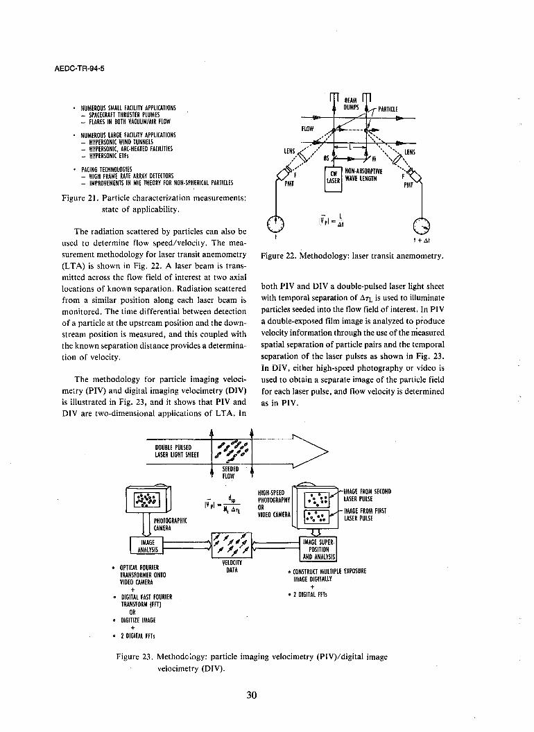
AEDC-TR-94-5

• NUMEROUS SMAll FACILITY APPLICATIONS - SPACECRAFT THRUSTER PLUMES - FLARES IN BOTH VACUUM/AIR FLOW

• NUMEROUS LARGE FACILITY APPLICATIONS - HYPERSONIC WIND TUNNELS - HYPERSONIC, ARC·HEATED FACILITIES - HYPERSONIC ElF!

PACING TECHNOLOGIES - HIGH FRAME RATE ARRAY DETECTORS - IMPROVEMENTS IN MIE THEORY FOR NON·SPHERICAL PARTICLES

Figure 21. Particle characterization measurements: state of applicability.

The radiation scattered by particles can also be used to determine flow speed/velocity. The mea­surement methodology for laser transit anemometry (L T A) is shown in Fig. 22. A laser beam is trans­mitted across the flow field of interest at two axial locations of known separation. Radiation scattered from a similar position along each laser beam is monitored. The time differential between detection of a particle at the upstream position and the down­stream position is measured, and this coupled with the known separation distance provides a determina­tion of velocity.

The methodology for particle imaging veloci­meay (PIV) and digital imaging velocimetry (DlV) is illustrated in Fig. 23, and it shows that PIV and DIV are two-dimensional applications of L T A. In

DOUBLE PULSED LASER LIGHT SHEET

• OPTICAL FOURIER TRANSFORMER ONTO VIDEO CAMERA

+ • DIGITAL FAST FOURIER

TRANSFORM (FFT) OR

• DIGITIZE IMAGE +

• 2 DIGITAL FFT!

SEEDED FLOW

_ dsp

IVpl- ~ ATl

FLOW

" •• :":;" LENS M. \,'<. .. '\,

NON·ABSORPTIVE " WAVE LENGTH

t+At

Figure 22. Methodology: laser transit anemometry.

both PIV and DlV a double-pulsed laser light sheet with temporal separation of ~1"L is used to illuminate particles seeded into the flow field of interest. In PIV a double-exposed film image is analyzed to produce velocity information through the use of the measured spatial separation of particle pairs and the temporal separation of the laser pulses as shown in Fig. 23. In DIV, either high-speed photography or video is used to obtain a separate image of the particle field for each laser pulse, and flow velocity is determined as in PIV.

HIGH·SPEED PHOTOGRAPHY OR VIDEO CAMERA

IMAGE FROM SECOND LASER PULSE

IMAGE FROM FIRST LASER PULSE

• CONSTRUCT MULTIPLE EXPOSURE IMAGE DIGITALLY

+ • 2 DIGITAL FFT!

Figure 23. Methodc:ogy: particle imaging velocimetry (PIV)/digital image velocimetry (DlV).

30

LASER AND INPUT OPTICS

OUTPUT SIGNAL

TIME

FRINGE PATTERN PARALLEL TO BISECTOR OF 0

dL ______ _ T------,

ED PARTICLE

AEDC-TR-94-5

OR

VF = (Pm - PB) df

PB '" BRAGG CELL FREQUENCY

Figure 24. Methodology: laser doppler velocimetry (LDV).

Perhaps the most well-known particle scattering technique for determination of flow velocity is laser Doppler velocimetry (LDV), and the methodology for its application is shown in Fig. 24. A laser beam is split into two components and crossed at a common focal point within a particle-seeded flow. An interference fringe pattern is created at the focal point with the pattern being parallel. to the bisector of the angular separation of the two laser beam com­ponents. An optical filter/photomultiplier system monitors the burst of scattered radiation as a particle passes through the fringe pattern. Through know­ledge of the fringe separation and the frequency of the scattered radiation pulses, a determination of flow velocity can be made. Other components of flow velocity can also be determined using different laser wavelengths in orthogonal planes. An excellent re­view of the details of LDV can be found in Ref. 22

The relative advantages and disadvantages of the particle scattering velocity measurement methods are tabulated in Fig. 25. The PIV and DIV methods offer near-instantaneous, wide-area coverage, There are directional ambiguity problems with PIV, and three­dimensional flow is a problem for both techniques. DIV has the capability for real-time measurements. To obtain multiple velocity components with PIV or DIV, multiple laser sheets and imaging systems must be used. LDV can much more readily obtain mUltiple velocity components, but instantaneous, wide-area coverage is sacrificed. In all cases the flow field must be seeded with small particles of known and fixed

31

METHOD ADVANTAGES DISADVANTAGES

PlY NEAR INSTANTANEOUS MEASURE- REQUIRES FLOW SEEDING WITH MENT OVER A WIDE AREA REVEALS FLOW STRUCTURE

SMAll « ll'm) PARTICLES

DIRECTIONAL AMBIGUITY MUST BE RESOLVED

3·D FLOW IS A PROBLEM

NO REAL·TIME CAPABILITY

DIV NO DIRECTIONAL AMBIGUITY REQUIRES FLOW SEEDING WITH PROBLEM SMALL « ll'm) PARTICLES

REAL-TIME CAPABILITY

NEAR INSTANTANEOUS MEASURE· 3·0 FLOW IS A PROBLEM ME NT OVER A WIDE AREA REVEALS FLOW STRUCTURE

tOV i-D, 2·D, 3·0 CAPABllI1Y WiTH NO INSTANTANEOUS WIDE AREA HIGH SPATIAL RESOLUTION (OVERAGE

REQUIRES FLOW SEEDING WITH SMALL « fl'm) PARTICLES

Fig. 25. Particle scattering:velocity measurement.

size, presenting a significant challenge for most hypersonic flows.

The state of applicability (see Fig. 26) for PIV and DIV has been limited to small-scale laboratory, transonic, and supersonic flow. 23-26 LD V and L T A have, on the other hand, been successfully applied to large-scale transonic, supersonic, and hypersonic facilities. 27, 29 However, particle seeding methods and the particle lag problem continue to prevent low uncertainty measurements in many regimes. An

AEDC-TR-94-5

PIV/DIV: SMALL SCALE, LABORATORY TRANSONIC, SUPERSONIC FLOWS

LDV/LTV: LARGE SCALE, TRANSONIC, SUPERSONIC, HYPERSONIC FACILITIES

PACING TECHNOLOGIES:

• PARTICLE SEEDING METHODS • PARTICLE LAG PROBLEM • DATA ACQUISITION ELECTRONICS

Figure 26. Particle scattering: velocity measurement state of applicability.

interesting approach to both problems has been advocated in Ref. 30, and this requires the use of larger, low specific gravity particles rather than the normal approach of smaller, higher specific gravity particles. Particularly associated with LDV is the need for improved data acquisition electronics to handle the high frequencies and data rates of hypersonic flows.

Absorption

Laser and lamp absorption techniques are receiving increased attention as a result of technological strides in laser scanning and UV resonance lamps. The laser absorption principle and methodology are illustrated in Fig. 27. Either a scanlJing ring dye or diode laser beam is split into two components and transmitted through the flow field of interest. Orie of the components is transmitted normal to the flow direction, and the other is transmitted at an angle (h to the flow direction. Typically, a pair of rotational absorption lines of a selected flow species is rapidly scanned ( "" 250-100 p.sec, and the absorption line profile is measured and normalized by the incident laser beam

intensity. The speCtral separation between absorption peaks scanned with the two beam components yields a measurement of flow velocity along the nonnormal beam using the Doppler shift relationship (see Fig. 27). By fitting one of the normalized line pair spectral profiles with the output of a computational model of the laser absoprtion process for the selected species, the species number density, rotational temperature, and static pressure can be determined. The number density is obtained through use of a cali­bration and the strength of the absorption measured; rotational ·temperature is obtained through the relative absorption strengths of the line pair and the Doppler broadening effect; static pressure is obtained through the collision broadening effect. Reference 31 provides an excellent review of the laser absorption methods.

The UV lamp absorption principle and methodo­logy are illustrated in Fig. 28. The lamp is selected to produce a spectrum resonant with a selected flow species. Lamp radiation is transmitted across the flow field, and the absorption spectra are recorded using a small spectrometer and array detector. Spectra are obtained with no flow (lamp shutter closed and open), and flow (shutter closed and open). This permits calculation of the spectral transmittance which can be related to the selected species number density through a calibration. Reference 32 provides an overview of lamp absorption methodology.

The advantages and disadvantages' of the absorp­tion methods are tabulated in Fig. 29. Although the lamp absorption method is simple, low cost, and valuable, it is limited to s'pecies concentration

A ......, ___ =~

LASER -.......,H~--I'"?'...-::::+------!--rl BEAM I

(SCANNING RING DYE A OR DIODE

LASER)

III 1'2 ABSORPTION LINE PAIR PROFILE OF SPECIES [x)

I, - 8, = 90 •

.... 82<90·

~ TIME (LASER FREQUENCY)

~ONE LINE PAIR - EXPT. V _ .:\.PD ( ..... COMPUTATIONAL F - P~ (O! 8 . MODEL

nIx), T, p FROM COMPUTATIONAL MODEL LASER FREQUENCY OF SPE(IES [x) ABSORPTION

Figure 27. Laser absorption.

32

AEDC-TR-94-5

I):: LENs-L----{~~:-l-----~NS- FILTER g-:~~h~~--- ----- ------JL:::.;;L-~_-_-_-~...;.;.:.;;;

meters. It must be noted that both techniques are LOS measurements, and a validated/calibrated computational model of the absorption process must be available for data reduction and analysis.

UV lAMP

~,"I"~'L:~'l~~. ~·L h h h

The state of applicability of the absorption techniques is evaluated in Fig. 30. Although most applications have been in small, laboratory shock tubes33.35 and burners,36 there have been some significant large facility successes. The lamp absorption method has been applied in the exhaust of a supersonic aircraft engine,37 in a NASA Langley arc-heated tunnel,38 and the AEDC HI and H2 arc-heated facilities.

FLOW EMISSION NO·FLOW SIGNAL NO·FLOW BACKGROUND (SHUTTER CLOSED) (SHUTTER OPEN) (SHUTTER CLOSED)

FLOW SIGNAL (SHUTTER OPEN)

TRANSMITTANCE (h) - nIx) THROUGH CALIBRATION

Figure 28. UV lamp absorption.

LASER ABSORPTION

ADVANTAGES

RELATIVELY SIMPLE, LOW COST IF USING DIODE LASERS

MULTIPLE MEASUREMENTS IN ONE APPARATUS CONFIGURATION: T, p, V, n

4·10 KHz SCANNING SPECTRAL REGIONS OF INTEREST

DISADVANTAGES

LOS

COMPLEX, EXPENSIVE IF USING SCAlI· NING RING DYE LASER WHICH AlSO HAS INSTABILITIES

MUST HAVE VALIDATED/CALIBRATED COMPUTATIONAL MODEL OF AIiSORp· TION PROCESS

DIODE LASER APPLICATIONS LIMITED 10 > 0.2 aIm

UV LAMP ABSORPTION

RELATIVElY SIMPLE, LOW COST • LOS (line·ol·Sight)

• VALUABLE TO APPLICATION Of • LIMITED TO nIx) MEASUREMENT LOCAL MEASUREMENTS

MUST DEAL WITH FLOW SElF·EMISSION

MUSi HAVE VAiiDAiED/CAliBRATED COMPUTATIONAL MODEL

DATA RATE LIMITED 10 ARRAY DETEC· TOR SCAN RATE (- 60 Hz)

Figure 29. Absorption measurements.

measurement and a data rate equal to the array detector scan rate. Furthermore, the lamp absorption method can be compromised by strong flow self­emission because of the limited spectral radiance of the lamp. The laser absorption method can become. complex and expensive when using a scanning ring dye laser system, but the low cost of a diode laser system presents a good alternative for flow conditions with static pressure greater than 0.2 atm. Perhaps the greatest advantage of the laser absorption method is its ability to provide measurement of multiple para-

33

The laser absorption method has been used in the NASA Ames 40-cm shock tunnel. 39 Both techniques will be

applied in the AEDC Impulse Facility within the year. Laser stability is a major problem, especially for the ring dye laser systems, and the lack of high scan rate array detectors limits the use of the lamp absorption method. Both methods have increased uncertainties because of a lack of accurate high-temperature spectroscopic parameters.

• NUMEROUS SMALL FACILITY APPLICATIONS; - SHOCK TUBES - FREE JETS

SOME LARGE FACILITY SUCCESSES: - SUPERSONIC AIRCRAFT ENGINE - NASA AMES 16·INCH SHOCK TUNNEL - NASA LANGLEY ARC·HEATEO TUNNEL - AEOC H·I/H·2 ARC·HEATED FACILITIES - DOTH TECHNIQUES WILL BE APPLIED TO AWC IMPULSE FACILITY FOR NITRIC

OXIDE A MEASUREMENTS

PAClt/G TECHNOLOGIES: - STABLE LASERS - HIGH SCAN RATE ARRAY DETECTORS - ACCURATE SPECTROSCOPIC PARAMETERS FOR HIGH T

Figure 30. Laser/lamp absorption: state of applicability

Line Reversal

One of the oldest nonintrusive diagnostic techniques is line reversal, and the basic principles are illustrated in Fig. 31. Numerous atomic species such as sodium and potassium have energy levels in near resonance with vibrational levels of major test facility flow species such as nitrogen. Using sodium and nitrogen as an example, the nitrogen molecules in a high vibrational level interact with ground state sodium atoms and produce sodium atoms in an excited level from which spontaneous emission can

AEDC-TR-94-5

17 16 15

32P3/2 , 1/2 V = 7 >-!:::

I 14 ~ 1:i 13

l-

V = 6 ;;: >-' 12 42p ~11 V = 5 312,112 as ----

400 v = 0

Na (32S1/2) N2X1/2 K(42Slnl

PARTIAL ENERGY LEVEL DIAGRAM LOG ng

SODIUM INTERACTION PROmS:

k12 Na(32S1/2) + N2 (v = 7, 8) :

k12

Na(32 P3/2 1/2) + N2 Iv = 0) ± 5E , A 2 21 2 -

Na(3 P3/2,1/2) - Na(3 S1/2) + heA21

(a SI Ba N~ li K

I

500 600 700 800

WAVELENGTH, nm

20 ng = N2 NUMBER DENSITY, (M-3

19 Tv (N2) = 2,000 K

18

17

16

15

141-...I........J~...I........JL........I.......I_ .... 1,000 1,200 1,400 1,600 1,800 2,000

Tex,INa), K

{, (,

900

Figure 31. Line reversal basic principles.

occur. Although there are times when the atomic species occur naturally within the flow, flow seeding

. with detectable atoms may be required. Provided that the number density of the molecular resonance species is sufficiently high to produce an adequate number of collisions between nitrogen and sodium, for example, the excitation temperature of sodium is nearly equal to the vibrational temperature of nitrogen. A detailed review of the line reversal technique may be found in Ref. 40.

The line reversal measurement methodology is illustrated in Fig. 32. Radiation from a broadband source such as a tungsten ribbon lamp is transmitted across the flow field of interest. The optical arrangement actually images the lamp ribbon at a selected point in the flow, and this image is sub­sequently split between two photomultipliers. A knife edge is inserted as shown in Fig. 32 such that one photomultiplier does not detect lamp radiation, only flow emission. Optical filters are used to isolate radiation detected to the area around the atomic emission line of interest. One photomultiplier pro­vides two signals: one signal is proportional to the sum of flow and lamp radiation and the other only lamp radiation with no flow. The other photo­multiplier monitors only lamp radiation. A signal ratio is formed as shown in Fig. 32, which can be used with a measurement of the lamp brightness temperature to produce a determination of vibra­tional temperature using the relationship given in Fig. 32.

34

L--__ S3 = (b'FLOW

S3

T lAMP = LAMP BRIGHTNESS TEMPERATURE, K

(2 = 1.4388 (M • K

Figure 32. Line reversal measurement methodology.·

The major advantages of the line reversal technique are its simplicity, high temporal resolution, and the information it provides on thermal non­equilibrium (Fig. 33). Unfortunately, it is an LOS technique and is susceptible to boundary-layer and particle effects. Flow seeding may be difficult for some applications, and the technique is certainly not applicable to the rarefied flow regime.

ADVANTAGES

• RELATIVELY SIMPLE, LOW (OST

• HIGH TEMPORAL RESOLUTION

• DETERMINES Tv

DISADVANTAGES

LlNE-OF,SIGHT - BOUNDARY -LAYER EFFECTS - PARTICLE EFFECTS

• MAY REOUIRE SEEDING

• COLLISIONAL EFfECTS

Figure 33. Line reversal measurements.

NUMEROUS SMALL FACILITY APPLICATIONS - FLAMES, BURNERS - SHOCK TUBES

SHOCK TUNNEl APPLICATION IN AWe TUNNEl I

PLANS FOR APPLICATION IN AEOC IMPULSE FACILITY

PACING TECHNOLOGIES: - FLOW CLEANLINESS - CAPABILITY OF COMPUTATIONAL MODEL OF MEASUREMENT PROCESS

Figure 34. Line reversal: state of applicability.

Most applications of line reversal have been in laborat~ry flames and burners41 , 42 and shock

tubes.43,44 There has been a large facility application in the former AEDC hypersonic Tunnel I, and there are plans for use of the technique in the AEDC Impulse Facility. Flow cleanliness and the capability of a computational model of the measurement pro­cess to provide data analysis are the major techno­logical limitations.

ENERGY

IONIZED ELECTRONIC STATES

EXCITATION PATH

LOWER ELECTRONIC STATE

---0 HIGH ENERGY nEURONS

t

AEDC-TR-94-5

Fluorescence

The basic· principles of the electron beam fluorescence (EBF) technique are illustrated in Fig. 35. This is an inelastic, local technique. A beam of high-energy (20-50 Kev) electrons provides excitation/ionization of molecules within the beam path, and as the excitedlionized molecules spontaneously decay to lower levels, fluorescence is produced with gas species specific characteristics. Collisional quenching of the excited/ionized levels is also present. Under moderate spectral resolution, the ro-vibrational bands of various species are easily distinguished, and high resolution of a particular band easily reveals the rotational structure.

The EBF temperature and number density measurement methodology is illustrated in Fig. 36. Because the electron beam must be generated under high vacuum (10- 7 torr, 1.33 x 10- 5 Pa), a multiple-stage dynamic pumping system must be used to inject the beam into the relatively high-pressure flow field of interest. The beam can be continuous or modulated, and the beam must be collected after transmission through the flow with a Faraday cup which monitors the beam current. Radiation from a point along the beam is collected, filtered (broad­band), and split into two components. Small spectro­meters or narrowband filters are used for spectral isolation of the fluorescence bands desired. Either a

KO-VIBRATIONAL BANDS MODERATE RESOLUTION

X, nm

'HIGH RESOLUTION

X, nm

Figure 35. Electron beam fluorescence (EBF) basic principles.

35

AEDC-TR-94-5

re:Gii~=l=+--------,,~~ ___ -.:::r-=-!=::::::j.,FARADAY CUP ; \ CONTINUOUS OR : '. MODUlATED e·BEAM

TURBO· PUMPS ~LENS

~ _____ .."...___ ___ BROADBAND FILTER

M I I

I :: BS ---;----------- I

I I I I

LENS A P, LENS \,' \,1

SMALL SPECTROMETER 9 9 SMALL SPECTROMETER OR NARROWBAND FILTER DR NARROWBAND FILTER

PMT OR ARRAY DETECTOR PMT OR ARRAY DETECTOR

S~f S~f ( Ib nIX) I GM(TR, Ty, >.) Us (A - >'s) d>. (

S.bf(As) = = I nIx), TR, Ty) . 1 + Qt(n(X), TR) 7{X)

FOR MODERATE RESOLUTION: s~f/s~f = I(Ty)::::' Ty

FOR LOW RESOLUTION: s~f/s~f = f(TR)::::. TR

FOR KNOWN TR, Ty: S~~ ~ nIX)

Figure 36. Electron beam fluorescence (EBF) measurement methodology.

FLOW

PULSED e- BEAM SYSTEM TIME DElAY BETWEEN PULSES IS T eb

FLOW

HIGH FREQUENCY SWEEP (OILS

longer linear, but number densities can still be determined using an iterative process. Obtaining number density mea­surements in the nonlinear signal region for a gas with more than three species is extremely diffi­cult. Reference 46 provides an excellent review of the EBF technique.

The EBF methodology for velocity measurement and flow visualization is illustrated in Fig. 37. There are two well-known velocity measurement techni­ques, and each requires the use of a pulsed electron beam. If a Langmuir probe is located a known distance downstream from the beam path across the flow field, then the time dffferen­tial between the pulse of'the elec-

PlASMA (OLUMNS

VELOCITY MEASUREMENT

FLOW VISUALIZATION

t? LENS V INTENSIFIED ARRAY

hotomultiplier or array detector is used, and the measured signal, Sebf (As), is given in Fig. 36 for a single species, x, for example. For a given beam current, the signal is a complex function of species number density, rotational temperature, and vibrational temperature. The func­tion GM(T R, T v,A) depends on the excita­tion/ emission model and the Boltzmann factors for the ro-vibrationallevels of the ground state molecules, and the variable gs(A - As) is the spectrometer or filter transmission function. The collisional quenching rate is Qc(n(x),Tr) and 7(X) is the lifetime of the excited state of species x. Following proper selection of spectral resolution and spectral position of the spectrometers or filters, a ratio of signals from the measurement channels can be predominantly a function of either rotational or vibrational temperature. With the measurement or knowledge of

e- GUN SYSTEM

Figure 37. Electron beam fluoresence (EBF) measurement methodology.

temperature and a calibration procedure, the signal from either channel can be used to determine species number density, n(x). For number densities less than 1015 molecules per cm3, the collision·al quenching effects can be ignored, and the fluorescence signal is a linear function of number density. For number densities between 1015 and 1017

molecules per cm3, the fluorescence signal is no

36

tron beam and the arrival of the plasma column at the Langmuir probe yields a determination of the flow velocity. An intensified array detector system can be located downstream of the pulsed beam to image the movement of the plasma columns. With a fixed, known time delay between beam pulses and knowledge of the separation of the plasma columHs from the imaging detector, flow velocity can be

POTENTIAL ENERG!

UPPER ElECTRONIC STATE

~ FLUORESCENCE

W GROUND ELECTRONIC STATE

INTERNUClEAR DISTANCE

S,

S, = CWFyfBn(x)VoT

Fa = Fa(T R' Tv) Am' Fy = .,----=----":"--=­

"'+Q(+ Qpre+ Oph

W = (PL/Ab)(XL/hc) k.GoL

AEDC-TR-94-5

Figure 38. Laser-induced fluorescence (LIF) basic principles.

determined. Flow visualization is easily accomplished with the use of high-frequency, magnetic sweep coils placed at the output of the electron gun system as shown in Fig. 37. Again, an intensified array detector system is used for imaging of the fluorescence field.

The basic principles of las!!r-induced fluorescence (LIF) are illustrated in Fig. 38. For LIF a laser beam rather than an electron beam

the laser power, Ab is the cross-sectional area of the laser beam, ka is the spectral absorption coefficient per molecule, and GOL is the overlap integral aCClJunting for the spectral lineshapes of the laser source and the excitation transition.

s,

'

A '" .., FLOW

~~~~ ~8~s~ \ ?!t\<~ is used to selectively excite molecules of a particular species to upper energy levels. Subsequent decay of the molecules to lower levels produces a fluorescence spectrum that lies to the long-wavelength side of the laser wavelength.

1/' / ~ PAIRS: ..... ----:::: .... 41.'7"'-4-;------'----

PUlSE1-Xu / i \ PULSE 2 - XL2 :', IMAGING

The fluorescence signal, Sr. is proportional to the excitation rate from the lower to the upper molecular level, W; the quantum yield of the upper molecular level, Fy; and the Boltzmann fraction for the lower molecular level, FB. The dependence on rotational and vibrational tem­perature is through the Boltzmann fraction, and the quantum yield is simply the ratio of the

, , OPTICS ~ '. f , . •",

Sfl S = fIT"~ Tv) ~ TR, Tv '2 FOR KNOWN TR, Tv

Sfl,2=>11(X)

INTENSIFIED ARRAY DETECTOR

fluorescence emission rate from a particular Figure 39. Laser-induced fluorescence (LIF) measurement group of individual transitions to the total decay methodology. rate from the upper level. The total decay rate can consist of spontaneous transition to all allowable. lower energy levels, coIIisional quenching, pre­dissociation, and multiphotoionization. The excita­tion rate, W, under the assumption of non-depletion of the ground state energy levels and a uniform laser pulse is given by the relation in Fig. 38 where PL is

37

The measurement methodology for LIF is illustrated in Fig. 39 for a particular variation called planar laser-induced fluorescence (PLIF). A pulsed laser beam is formed into a laser sheet with the use of a combination of spherical and cylindrical optical elements, and the beam is transmitted across the flow field of interest. The laser sheets are normally

AEDC-TR-94-5

generated in pairs of pulses, each at a different wavelength, and temporally separated by 100-200 nsec. The sheets of fluorescing gas are imaged onto a pair of intensified array detectors. A pixel-to-pixel ratio of fluorescence signals for the laser pulse pairs is a function of rotational and vibrational tempera­ture. If the excitation transitions selected are from different vibrational levels but identical rotational levels, then the intensity ratio is. a function of vibrational temperature. Similarly, if the selected excitation transitions originate from identical vibra­tionallevels but different rotational levels, then the intensity ratio is a function of rotational temperature. Usually, a combination of calibration and com­putational model will be required for data reduction and analysis. Following determination of tempera­tures, species number densities can be determined from either of the fluorescence signals with the use of a calibration and a computational model. This assumes that a strategy has been successfully devised to either eliminate or to provide a correction for the collisionai quenching effects. As noted earlier, the use of predissociative upper levels or multi­photoionization can eliminate collisional quenching effects. Two methods available for producing a collisional quenching correction are measurement of the upper level total decay rate by monitoring the temporal variation of the fluorescence signal following the laser pulse, or calculation of the quenching effects through use of independent mea­surement of all flow species concentrations and a compilation of collisional quenching cross sections for all flow species. The latter approach is not too practical for most hypersonic applications.

DOPPLER-SHIFT VElOCITY MEASUREMENT:

flOW

PULSED LASER BEAM

(Sr/E~) - (Sr/E~

(Sr/E~) + (Sr/E~

11

RETRO-REflECTlNG OPTICAL TIME DELAY

RELATIVE LINE SHAPE

A methodology for measurement of flow velocity using LIF is illustrated in Fig. 40. A pulsed laser beam is transmitted. across a flow field at a known angle (), and following a time delay of loo-2oo nsec is retro­reflected back across the flow field. Fluorescence is collected from a point along the path of the beams, optically filtered, and detected by a photomultiplier tube. If the laser linewidth, o~, the spectral separa­tion of laser wavelength and absorption transition for no flow, d~L' and the width of the absorption transition, o~, meet the inequality given in Fig. 40, then an algorithm for measurement of flow velocity can be formed. This algorithm is based on the Doppler shift of the absorption transition as illustrated in Fig. 40. The algorithm uses the ratio of the difference and sum of the energy normalized fluorescence signals for the forward and backward propagating laser beams, and this is equal to the ratio of the difference and sum of the overlap integrals for the forward and backward propagating laser ?eams.

The major advantages for the EBF technique are its strong signals, its multiple parameter measurement capability, and, for some applications, its ability to produce a signal from all flow species. Unfortuna­tely, collisional quenching limits its applicability to total number densities less than 1017 cm - 3, and beam spreading effects at densities greater than l()16

cm - 3 can limit applicability to transmission lengths less than loo cm. As noted previously, multiple stage pumping is required for beam injection into the flow, and high levels of cleanliness must be maintained for stable gun operation. There are also safety issues related to the use of high voltage and creation of X-

ABSORPTION LINE SHAPE, r NO flOW

LASER LINE SHAPE

Figure 40. Laser-induced fluorescence (LIF) measurement methodology.

38

rays. One of the major advantages for the LIF techni­que in some applications is its ability to selectively excite flow species. It can also provide wide spatial coverage with high temporal resolution as well as multiple measurement parameters. Special strategies must be devised to deal with the collisional quenching problem, and multiple laser pulses may be required to achieve the desired measurement precision. Figure 41 tabulates the advantages and disadvantages of EBF and LIF.

EOF

ADVANTAGES DISADVANTAGES

• ALL FLOW SPECIES EXCITEDIIONIZED • COLLISIONAL QUENCHING LIMITS DEN· TO GIVE AN EMISSION SIGNATURE SITY MEASUREMENT TO "r < 1011

(m-3

STRONG SIGNALS MEAN APPLICABILITY • BEAM SPREADING EFFECTS AT nl ;;, IN RAREFIED FLOW REGIME, 1016 (m-3 LIMIT APPLICATION TO A nls 1016 (m-3 BEAM TRANSMISSION LENGTH OF <

100 (m

CW NATURE OF BEAM PERMITS STUDY • MULTIPLE STAGE PUMPING REQUIRED OF TURBULENCE FOR INIEGION INTO FLOW (PRESSURE

IN a·GUN s 10-7 TORR)

• METHODS FOR V MEASUREMENT AND • HIGH LEVEL OF CLEANLINESS MUST BE FLOW VISUALIZATION AS WELL AS TR, MAINTAINED Tv, nIx)

LlF

• SELECTED SPECIES CAN BE EXCITED TO PRODUCE AN EMISSION SIGNATURE

WIDE SPATIAL COVERAGE WITH HIGH TEMPORAL RESOLUTION

• METHODS FOR TR, Tv, nIx), v, AND FLOW VISUALIZATION

SAFETY ISSUES; HIGII VOLTAGE, X·RAYS

STRATEGIES 'MUST BE EMPLOYED TO DEFEAT COLLISIONAL QUENCHING PROBLEM (e.g. PREDISSOCIATION, PHOTOINIZATlON, DIRECT MEASURE· MENT OF EMISSION RATE)

MULTIPlE PULSES MAY BE REQUIRED TO ACHIEVE DESIRED MmUREMENT PRECISION

Figure 41. Fluorescence measurements.

• NUMEROUS SMALL FACILITY APPLICATIONS - SIMULATED SPACECRAFT THRUSTER PLUMES - MONO· AND OI·PROPELLANT THRUSTER PLUMES - SIMULATED PLANETARY ATMOSPHERES - STUDIES OF CONDENSATION

NUMEROUS LARGE FACILITY, RAREFIED FLOW APPLICATIONS - AEDC ARC·HEATED FLOWS . - AEDC RESISTANCE·HEATED HYPERSONIC TUNNEL - BOEING SHOCK TUNNEL - GE TEST FACILITIES - FRENCH FACILITIES - GERMAN FACILITIES

FLIGHT MEASUREMENTS - HIGH ALTITUDE SOUNDING ROCKETS - SHUTTLE ORBITER BAY - HE·ENTRY BOUNDARY LAYER FLIGHT EXPERIMENT

• PACING TECHNOLOGIES; - HIGH ENERGY, HIGH CURRENT GUN SYSTEMS - HIGH FRAME RATE ARRAY DETECTORS

Figure 42. Electron beam fluorescence: state of applicability.

39

AEDC-TR-94-5

Because the EBF technique has been in use since the early 1960s, the technique has achieved a mature state of applicability (see Fig. 42). The small facility applications include studies of simulated spacecraft thruster plumes,47 simulated chemical laser flow fields,48 mono-and bipropellant thruster plumes, simulated planetary atmospheres, studies of con­densation phenomena, and low-density hypersonic flows. 49, 50 With regard to large facility applications, AEDC has used the technique in both arc-heated and resistance-heated hypersonic tunnels and a recent application in the Boeing 76-cm hypersonic shock tunnel. 51 There have also been numerous applications in the General Electric aerospace facilities (Ref. 52, for example). Both German and French researchers have recently used the technique in hypersonic facilities. 53 , 54 Indeed, the EBF technique has been used for flight measurements that include high-altitude sounding rockets, the shuttle orbiter bay, and a reentry boundary-layer flight experiment. The EBF technique could achieve even more applicability with development of user-friendly high-energy, high-current electron gun systems and high frame rate array detectors.

• NUMEROUS SMALL FAClLliY APPLICATIONS '- BURNERS - SHOCK TUBES - FREE JET EXPANSIONS - SUPERSONIC TUNNEL

• LIMITED LARGE FACILITY SUCCESSES - GERMAN AND NASA ARC·HEATED FACILITIES - FREE·fLIGHT HYPERVELOCITY RANGES ' - SHOCK TUNNELS - ROCKET EXHAUST PLUMES

• PACING TEHCNOLOGIES - LASER SYSTEMS - ACCURATE COMPUTATIONAL MODELS OF EXCITATION/EMISSION PROCESS - HIGH FRAME RATE ARRAY DETECTORS

Figure 43. Laser-induced fluorescence: state of applicability.

The LlF technique has been primarily limited to small facility applications, but there have been a few large facility successes as noted in Fig. 43. The small facilities include burners, 55, 56 shock tubes,57 free jet expansions,58 and small supersonic tunnels. 59, 60 The large facility applications include German and NASA arc-heated facilities,61, 62 free-flight hypervelocity ranges at AEDC,63 shock tunnels at Boeing,64 and rocket exhaust plumes. 65 There are three major pacing technologies: tunable, stable, narrow line, high pulse energy, high pulse rate laser systems; accurate computational models of the complex excitation/emission processes; and high frame rate array detectors.

AEDC-TR-94-5

POTENTIAL ENERGY,

CM-l

50,000

40,000

30,000

20,000

UPPER ElECTRONIC STATE

LOWER ELECTRONIC STATE

- - - - VIRTUAL STATE

10,000

O~~~--~~~~~~ o 0.5 1.0 1.5 2.0 2.5 3.0

INTERNUCLEAR DISTANCE, A

MOLECULAR ENERGY LEVU DIAGRAM

LASER ANTI· STOKES (olE > 0) LINE STOKES (AE < 0)

LASER LINE'

III

ON _ 00 N:z:C"'1CN _ _ : .....,0 :zvz::z:;:c:c

I : I I : I

: I

1,000. 2,000 3.000 4,000 5,000

A~ CM-l

HIGH RESOLUTION (ROTATIONAL RAMAN LINES)

- SPECIES Y --- - SPECIES X

: I I I

I I I I I I I I I I I I

! I I I I I I I

II , I I I I I I I I I

:1. I I : II

I I I I I I I

150

Figure 44. Spontaneous raman scattering basic principles.

Raman Scattering LASER BEAM >'l -i\------~r-r------::i3 BEAM DUMP

I' I' , The basic principles of Raman

scattering are illustrated in Fig. 44. The technique involves the inelastic interaction of laser photons with molecules which in-duce transitions to virtual states and the subsequent, nearly instantaneous decay to lower levels different from the original levels. This produces scattered photons with energies (wavenumbers) decreased or increased depending on the difference between the final and initial energy levels. The shift in wavenumber is molecularly specific as shown in Fig. 44. The ro­

: \ , 'L

I A o ~ PF

M /: _________ ~-;::INF /--~----~----y i ~ SMALL t-:

L '0 : SPECTROMETERS \; L

0" ::::: .. l~ ~ ~ DETECTORS

sam S~m

. OR

FB(TR) -:::::>TR

FOR KNOWN TR, Tv:

sa~-:::::> n(x)

vibrational Raman bands are nominally shifted 1,000-4,000 cm -I from the laser line. Traditionally, the negative wave­number shifts are termed anti-Stokes, and the positive wavenumber shifts are termed Stokes. Within a wavenumber region of

LOW RESOLUTION: SRm = CI. n(x)FB(Tv) I gRm (5:)g,(5: - 5:,)d5:

HIGH RESOLUTION: SRm = CI. n(X)Fo(T R) I hm (5:)g,(5: - 5:,)d5:

Figure 45. Spontaneous raman scattering measurement methodology.

150-200 cm - 1 around the laser line are the rotational Raman lines associated with rotational energy level transitions that do not involve a change in vibrational energy level. The major Raman scattering diagnostic methods are spontaneous Raman scattering and coherent anti-Stokes Raman scattering (CARS). References 66 and 67 provide details on the principles of spontaneous and Raman scattering and CARS, respectively.

40

The methodology for spontaneous Raman scattering is illustrated in Fig. 45. A laser beam is transmitted across the flow field of interest and captured by a beam dump system. Raman scattered radiation is collected from a point along the' beam path and, following polarization and rejection filtering to reject Rayleigh/Mie scattered radiation', the radiation is split into two components for final

spectral selection with small spectrometers or filters. Detection is usually provided by photomultipliers or array detectors. Selecting low spectral resolution, the measured signal from each detection channel is directly proportional to laser pulse energy and selected species number density. The signal is also a function of vibrational temperature and the overlap integral. For high resolution, i.e., detecting either the pure rolationallines or the rotational lines within a ro-vibrational band, the signal is a function of rotational temperature. A ratio of signals from the two detection channels can then be a function of either vibrational or rotational temperature. With measurement of temperatures, the signal from either channel can be used with a calibration to determine the selected species number density.

The basic principle for CARS is illustrated in Fig. 46. When two high power density laser beams of wavenumbers ~I and ~2 with the difference in wavenumbers equal to a Raman shift of a particular molecular species are brought together in an optically nonlinear medium containing the species, a coherent beam at the anti-Stokes wavenumber (~3 = 2~1 ->d is generated. The CARS beam is created through the third-order susceptibility and the high electric field strengths of the laser beams at the point of interaction. The CARS spectrum can be obtained by tuning the wavenumber of one of the lasers or by operating one of the laser beams in a broadband mode such that the complete spectrum can be

GROUND ELECTRONIC STATE

VIRTUAL LEVELS

AEDC-TR-94-5

obtained. To obtain maximum CARS signal, the phase matching requirements shown in Fig. 46 must be met. The wave vectors for the incident laser beams and the CARS beam are designated I( 1> 1(2, and 1(3, respectively. Phase matching can be obtained with collinear beams, but the method of choice because of its high spatial resolution is termed BOXCARS. The angles for beam crossings in the BOXCARS configuration are shown in Fig. 46. The beam crossings do not have to occur in a single plane. The BOXCARS wave vector diagram in Fig. 46 can be folded along the dashed line.

A measurement methodology for CARS is illustrated in Fig. 47, with a folded BOXCARS configuration used in this example. The two laser beams with wavenumber ~I lie in the plane of the figure, and the laser beam with wavenumber ~2 is above the plane of the paper. The laser beams are brought to a focus at the desired measurement point, and the created CARS beam emerges from the focal volume upwardly out of the plane of the figure. The value of this particular configuration is its ability to provide high spatial rejection of the incident laser beams from the detection system which can consist of a smali spectrometer or filter and it photo­mult1plier tube or array detector. The CARS signal is dependent on the intensities of the incident laser beams, the square of the third-order nonlinear susceptibility, and the square of the beam interaction

SPECTRUM

~!"N"" POTENTIAL F~~-" -~ INCIDENT ENERGY

-1I:i GENEIlATED

Az hi

INCIDENT -hi BROADBAND

~E = he(hl - Az) - - -~=2hl-Az

PHASE MATCHING REQUIREMENTS -K I • K I .. .. = K2 K3

COLLINEAR BOXCARS

Figure 46. Coherent anti-stokes raman scattering (CARS) basic principle.

41

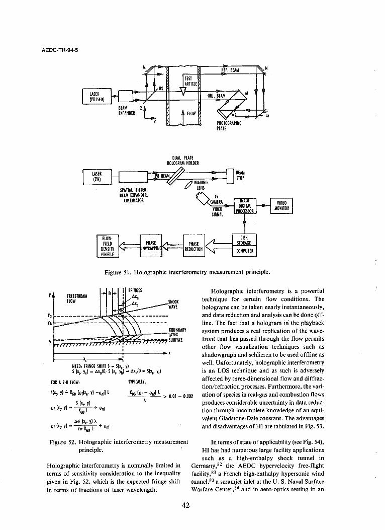
I

I

AEDC-TR-94-5

BEAM XL EXPANDER

Y

TEST ARTICLE

FLOW

PHOTOGRAPHIC PLATE

M

DUAL PLATE HOLOGRAM HOLDER

L..-_~_~_f ---'HL-----' 2BBEA~ : ~ tllMAGING LENS

DBEAM STOP

SPATIAL FILTER, BEAM EXPANDER,

COLLIMATOR

FLOW· FIELD

DENSITY PROFILE

PHASE PHASE DISK

STORAGE 1'V'--,INWRAPPINlj"r-----. REDUCTION COMPUTER

Figure 51. Holographic interferometry measurement principle.

Ya

Yb

FREESTREAM FLOW

FRINGES

SHOCK WAVE

~-----------------;-----------.x I------Xe ...:

NEED: FRINGE SHIFT S = S(xe• Y) S (xc' Yo) = /lxa'D; S (xc' Vb) = /lXb/D = S(x" Ve)

FOR A 2·0 FLOW: TYPICALLY.

S(~. y) ,;, IltiD [Qf(Ke. y) -Qntl L

S (~. y)

KoG (Qf - Qnf) L > 0.01 _ 0.002 A

Holographic interferometry is a powerful technique for certain flow conditions. The holograms can be taken nearly instantaneously, and data reduction and analysis can be done Qff­line. The fact that a hologram in the playback system produces a real replication of the wave­front that has passed. through the flow permits other flow visualization techniques such as shadowgraph and schlieren to be used offline as well. Unfortunately, holographic interferometry is an LOS technique and as such is adversely affected by three-dimensional flow and diffrac­tion/refraction processes. Furthermore, the vari­ation of species in real-gas and combustion flows produces considerable uncertainty in data reduc­tion through incomplete knowledge of an equi­valent Gladstone-Dale constant. The advantages and disadvantages of HI are tabulated in Fig. 53.

Qf (~. y) = ~ + Qnf

/l.p (xc' y) A Qf (xc' y) = 2?r IltiD L + Qnf

Figure 52. Holographic interferometry measurement principle.

Holographic interferometry is nominally limited in terms of sensitivity consideration to the inequality given in Fig. 52, which is the expected fringe shift

in terms of fractions of laser wavelength.

42

In terms of state of applicability (see Fig. 54), HI has had numerous large facility applications such as a high-enthalpy shock tunnel in

Germany,82 the AEDC hypervelocity free-flight facility,83 a French high-enthalpy hypersonic wind tunnel,83 a scramjet inlet at the U. S. Naval Surface Warfare Center, 84 and in aero-optics testing in an

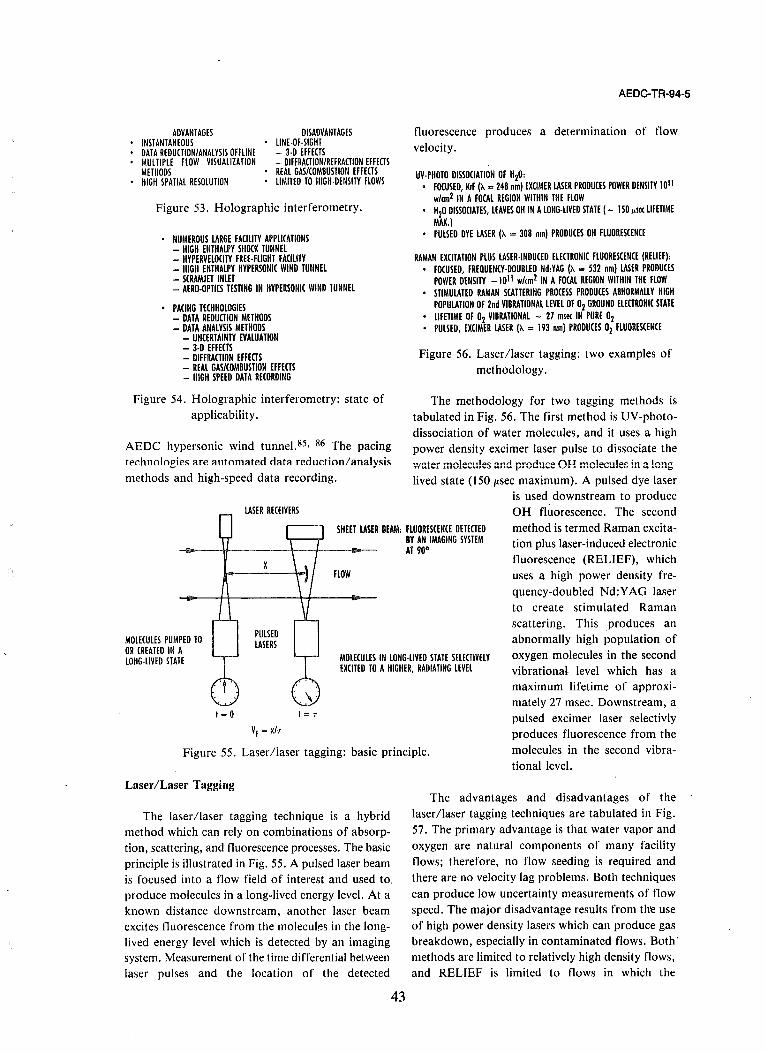
ADVANTAGES INSTANTANEOUS DATA REDUCTION/ANALYSIS OffLINE MULTIPLE fLOW VISUALIZATION METHODS HIGH SPATIAL RESOLUTION

DISADVANTAGES LINE-Of-SIGHT - 3-0 EFFECTS - DIFFRACTION/REFRACTION EFFECTS REAL GAS/COMBUSTION EFFECTS LIMITED TO HIGH-DENSITY FLOWS

Figure 53. Holographic interferometry.

NUMEROUS LARGE fACILITY APPLICATIONS - HIGH ENTHALPY SHOCK TUNNEL - HYPERVELOCITY fREE-FLIGHT fACIlITY - HIGH ENTHALPY HYPERSONIC WIND TUNNEL - SCRAMJET INLET - AERO-OPTICS TESTING IN HYPERSONIC WIND TUNNEL

• PACING TECHNOLOGIES - DATA REDUCTION METHODS - DATA ANALYSIS METHODS

- UNCERTAINTY EVALUATION - 3-D EFFECTS - DIFfRACTION EFFECTS - REAL GAS/COMBUSTION EFFECTS - HIGH SPEEO DATA RECORDING

Figure 54. Holographic interferometry: state of applicability.

AEDC hypersonic wind tunnel. 85. 86 The pacing technologies are automated data reduction/analysis methods and high-speed data recording.

AEDC-TR-94-5

fluorescence produces a determination of flow velocity.

UV-PHOTO DISSOCIATION Of "20: • FOCUSED, KrF (>. = 248 om) EXCIMER LASER PRODUCES POWER DENSITY 1011

wlcm2 IN A FOCAL REGION WITHIN THE fLOW "20 DISSOCIATES, LEAVES OH IN A LONG-LIVED STATE (- 1501'1« LIFETIME MAX.)

• PULSED DYE LASER (>. = 308 nm) PRODUCES OH FLUORESCENCE

RAMAN EXCITATION PLUS LASER-INDUCED ELECTRONIC fLUORESCENCE (RELIEf): • fOCUSED, FREQUENCY-DOUBLED Nd:YAG (>. = 532 nm) LASER PRODUCES

POWER DENSITY -1011 wlcm2 IN A FOCAL REGION WITHIN THE FLOW STIMULATED RAMAN SCATTERING PROCESS PRODUCES ABNORMALLY HIGH POPULATION Of 20d VIBRATIONAL LEVEL Of O2 GROUND ELECTRONIC STATE LIFETIME OF O2 VIBRATIONAL - 21 m!6( IN PURE 02 PULSED, EXCIMER LASER (>. = 193 om) PRODUCES O2 fLUORESCENCE

Figure 56. Laser/laser tagging: two examples of methodology.

The methodology for two tagging methods is tabulated in Fig. 56. The first method is UV-photo­dissociation of water molecules, and it uses a high power density excimer laser pulse to dissociate the water molecules and produce OH molecules in a long­lived state (150 /Lsec maximum). A pulsed dye laser

is used downstream to produce OH fluorescence. The second

SHm LASER BEAM: FLUORESCEN(E DETECTED BY AN IMAGING SYSTEM AT 90·

method is termed Raman excita­tion plus laser-induced electronic fluorescence (RELIEF), which

FLOW uses a high power density fre­quency-doubled Nd: YAG laser to create stimulated Raman scattering. This produces an abnormally high population of MOLECULES PUMPED TO

OR CREATED IN A LONG-LIVED STATE MOLECULES IN LONG-LIVED STATE SELECTIVElY

EXCITED TO A HIGHER, RADIATING LEVEL oxygen molecules in the second vibrational level which has a maximum lifetime of approxi­mately 27 msec. Downstream, a pulsed excimer laser se1ectivly produces fluorescence from the

,= 0 ,= T

Vf = X/T

Figure 55. Laser/laser tagging: basic principle. molecules in the second vibra­tional level.

Laser/Laser Tagging

The laser/laser tagging technique is a hybrid method which can rely on combinations of absorp­tion, scattering, and fluorescence processes. The basic principle is illustrated in Fig. 55. A pulsed laser beam is focused into a flow field of interest and used to_ produce molecules in a long-lived energy level. At a known distance downstream, another laser beam excites fluorescence from the molecuks in the long­lived energy level which is detected by an imaging system. Measurement of the time differential between laser pulses and the location of the detected

43

The advantages and disadvantages of the laser/laser tagging techniques are tabulated in Fig. 57. The primary advantage is that water vapor and oxygen are natural components of many facility flows; therefore, no flow seeding is required and there are no velocity lag problems, Both techniques can produce low uncertainty measurements of flow speed. The major disadvantage results from the use of high power density lasers which can produce gas breakdown, especially in contaminated flows. Both' methods are limited to relatively high density flows, and RELIEF is limited to flows in which the

AEDC-TR-94-5

UV-PHOTODISSOCIATION OF H20 ADVANTAGES DISADVANTAGES

H20 IS A NATURAL COMPONENT OF 'NEED n(H20) - 10 17 cm-3

MANY FACILITY FLOWS 'GAS BREAKDOWN MAY OCCUR NO VELOCITY LAG PROBLEM 'lIFETIME OF OH HIGHLY DEFENDENT ONLY WEAK DEPENDENCE OF EXCITED ON COLLISION PARTNERS (e.g. H2) OH LIFETIME ON TEMPERATURE

RElIEF O2 IS A NATURAL COMPONENT OF 'lIMITED TO TEMPERATURE < 800 K MOST FACILITY FLOWS 'lIFETIME OF O2 VIBRATIONAL LEVELS NO VELOCITY LAG PROBLEMS HIGHLY DEPENDENT ON COlliSION HIGH PRECISION PARTNERS (e.g. H20)

'lIKElY LIMITED TO flOWS WITH TOTAL DENSITY EQUIVALENT TO I aIm

'GAS BREAKOOWN MAY OCCUR

Figure 57. Laser Ilaser tagging.

vibrational and rotational temperatures must be less than 800 K. The long lifetime levels used in each method have a lifetime dependence on their collision partners; therefore, care must be exercised in applica­tion of the methods in reacting or real-gas flows.

• NUMEROUS SMALL FACILITY APPLICATIONS - SUPERSONIC FREE-JET - VERTICAL, MACH 3 WIND TUNNEl

• NO KNOWN LARGE FACILITY APPLICATIONS • PACING TECHNOLOGIES

- HIGH POWER, SHORT PULSE LENGTH (picose[onds) LASERS - HIGH FRAME RATE ARRAY DETECTORS

Figure 58. Laser/laser tagging: state of applicability.

The state of applicability of the laser Ilaser tagging methods is assessed in Fig. 58. Although there are no known large facility applications thus far, there have been a few small facility applications. The disso­ciation of water method has been used, for example, in a supersonic free jet,87 and the RELIEF method' has been used in a vertical, Mach 3 wind tunnel. 88 The pacing technologies are high-power, short pulse length lasers to produce the high power densities required in large-scale facilites and high frame rate imaging systems.

METHODOLOGY OF DIAGNOSTICS SELECTION

With many methods available it is important to follow a process for selection of the best diagnostics technique or techniques to produce the data required. The first step is to clearly define the benefits sought -from the measurements and the type of experiments planned' as tabulated in Fig. 59. In other words, it is important to know exactly why the nonintrusive measurements are required.

44

(fO CODE VALIDATION - VERIFY CODE'S ABILITY TO MODEL flOW PHYSICS (fD CODE CALIBRATION - DETERMINE CODE'S ABILITY TO PREDICT SPECIFIC PARAMETERS FACILITY FLOW-FiElD CHARACTERIZATION - DETERMINE SPATIALITEMPORAL CHARACTERISTICS OF FREE-STREAM flOW

• PROPULSION SYSTEM PERFORMANCE CHARACTERIZATION - INlET MASS flOW, EXHAUST FUEL/AIR RATIO AERODYNAMIC FLOW-FiElD CHARACTERIZATION - TRANSITIONITURBULENCE PHYSICS BUILDING BLOCK EXPERIMENTS ,- PHENOMENOLOGICAL

• BENCHMARK EXPERIMENTS - PARAMETRIC DESIGN/CONFIGURATION EXPERIMENTS - ClOSE TO FLIGHT CONDITIONS

Figure 59. Methodology of diagnostic selection: define benefits/identify experimetns.

• DEFINE SETS OF PARAMETERS TO BE MEASURED • PRIORITIZE SETS • PRIORITIZE WITHIN SETS (IF REDUNDANT MEASUREMENTS) • SET OF UNCERTAINTY TARGETS/GOALS TARGET: THE UNCERTAINTY LEVEl WHICH, IF NOT MET, WILL PROVIDE NO USEFUL

INFORMATION GOAL: THE UNCERTAINTY LEVEL WHICH, IF DECREASED, WILL NOT IMPROVE THE

USEFULNESS OF THE INFORMATION

GOAL TARGET--......

Figure 60. Methodology of diagnostic selection: parameters/uncertainties.

The next step, as outlined in Fig. 60, is to clearly define the sets of parameters that must be measured, prioritize the sets and within ,sets, and establish uncertainty targets and goals. Here, the target is defined as the uncertainty level which, if not met, will provide no useful information, and the goal is the uncertainty level which, if decreased, will not improve the usefulness of the information.

SPATIAL RESOLUTION - NOMINAL 11100 OF NOZZlE EXIT PLANE DIAMETER, OF ENGINE INLET DIAMETER, OF MODEl SCALE, ETC.

• SPATIAL COVERAGE - TEST OBJECTIVE DEPENDENT • TEMPORAL RESOLUTION - NOMINALLY < I !,se[ FOR "INSTANTANEOUS"

MEASUREMENT, I Se! - 2 liSe! FOR TIME AVERAGE, TEST OBJECTIVE DEPENDENT DATA RATE - TEST OBJECTIVE DEPENDENT, MUST CONSIDER FACILITY RUN TIME, ON-CONDITION TIME, PHENOMENON TIME, UNCERTAINTY REQUIREMENTS SIMULTANEITY - TEST OBJECTIVE DEPENDENT

Figure 61. Methodology of diagnostic selection: set data requirements.

There are certainly other data requirements to be set besides uncertainty, and they are listed in Fig. 61. Spatial resolution, spatial coverage, temporal resolu­tion, data rate, and simultaneity of various measure­ments are usually test objective-independent. For

spatial and temporal resolution, there are some general rules that can be applied, as shown in Fig. 61.

MINIMUM UNCERTAINTY (ALCULATIONS

~ (OMPARISON TO REQUIREMENTS

PRELIMINARY SELECTIONS

Figure 62. Path to preliminary selections.

The next step, suggested in Fig. 62, requires surveying the techniques that can produce the data required and making minimum uncertainty calcula­tions· for each of the techniques identified. The minimum uncertainty calculations involve deter­mining the so-called quantum or shot-noise limit for the techniques. Those techniques that have minimum uncertainty within the required uncertainty levels are then assessed with regard to meeting the other data requirements, and a preliminary selection of techniques is accomplished.

(FOR EXAMPLE)

AEDC-TR-94-5

ing the level of risk, and defining methods for reducing the risk. Some of the previously selected techniques may have to be abandoned if no risk reduction measures can be identified.

Another critical step shown in Fig. 64 is a realistic consideration of the costs involved in application of the techniques identified thus far. The costs of feasibility determination, technology development and transfer, safety and facility operation, and life cycle must be analyzed.

FEASIBILITY DETERMINATION - ANALYTICAL/EXPERIMENTAL S(REENING - FEASIBILITY (ONFIRMATION

• TECHNOLOGY DEVELOPMENT - HARDWARE - SOFTWARE

• TECHNOLOGY TRANSFER - INITIAL TRAINING - INSTALLATION - TEST BED OPERATION SAFETY AND FACILITY OPERATION

• LIFE CYCLE - TRAINING - MAINTENANCE - UPGRADES

Figure 64. Methodology of diagnostic selection: cost considerations

With the previous steps completed, it is possible to .consider data productivity as shown in Fig. 65. Productivity is defined as the value of the data to be

obtained versus the projected cost of

TECHNICAL RISK RISK EVALUATION RISK REDUCTION EFFORTS obtaining the data. In assessing the value of the data, which can be a somewhat subjective process, it is recommended that consideration be given to the direct value of the data (I.e., the data were previously unobtainable), the cost savings of the data

LOW: MED: NOT (RITI(AL,

(RITICAL COUNTER-MEASURES IDENTIFIED

HIGH: (RITI(AL, MUST BE

DEMONSTRATED

(I.e., the diagnostic system has replaced an existing system), and the spin-offs or

hidden values produced by the data.

Figure 66 summarizes the diagnostics selection process, and it is important to note the usual need to consider trade-offs; that is, it might be important to relax some of the data and uncertainty require­ments in order to cut costs, to meet dead­lines, etc.

Figure 63. Methodology of diagnostic selection: risk considera­tions. (for example).

METHODOLOGY OF DIAGNOSTICS APPLICATION

The next step, risk consideration, is often ignored, unfortunately. Figure 63 is an illustration of the method used at AEDC for identifying risks, evaluat-

45

Figures 67-71 illustrate a method that can be followed for successful application of nonintrusive diagnostics. First, it is important to create a comprehensive, integrated strategy for the

AEDC-TR-94-5

PRODUCTIVITY: TOTAL VALUE OF RESULTING DATA VERSUS TOTAL COST 0 DIAGNOSTIC SYSTEM DIRECT VALUE (i.e. DATA PREVIOUSLY UNAVAILABLE) PRODUCTIVITY = VALUE OF DATAITOTAL COST COST SAVINGS (i.e. DIAGNOSTIC REPLACES EXISTING SYSTEM(s)) PRODUCTIVITY = SAVINGS + VALUE ADDED TO DATAITOTAL COST SPIN·OFFS (HIDDEN VALUES) - DATA LEADS TO NEW WORK - DEVElOPMENT PROCESS PRODUCES FRINGE BENEFIT - DIAGNOSTIC SYSTEM HAS OTHER APPLICABILITY

Figure 65. Methodology of diagnostic selection process: productivity considerations.

TEST PARAMETER

AND UNCERTAINTIES

MINIMUM UNCERTAINTY CALCULATIONS

Figure 66. Methodology of diagnostic selection: final selection(s).

THE PLAN: THE COMPREHENSIVE, INTEGRATED STRATEGY THAT THE DEVElOPMENT FOR APPLICATION PROCESS WILL FOLLOW.

- WORK BREAKDOWN STRUCTURE - SCHEDULE/LEAD TIME - CRITICAL PATH/POINTS - IDENTIFY/ESTIMATE COSTS - TRACKING

THE TEAM: THE PERSONNEl CRITICAL TO THE SUCCESSFUL EXECUTION OF THE PLAN - A SPAN OF SCIENTIFIC DISCIPLINES IS REOUIRED: PHYSICS, ElECTRICAl/

MECHANICAl/AEROSPACE/COMPUTATIONAL ENGINEERING, PHYSICAL CHEMISTRY, FACILITY OPERATORS, TECHNICIANS, .•.

- INTEGRATION AND COOPERATION IS A REQUIREMENT - COLLABORATION WITH OTHER GROU PS, NOT COMPETITION - SEEK SUPPLEMENTAL FUNDING

Figure 67. Methodology of diagnostics application: planning/teaming.

application-specific development --- the plan. This plan should at the very least include the following

46

DIAGNOSTIC COMPUTATIONAL MODEL: A COMPREHENSIVE MODEl OF THE MEASURE­MENT PROCESS, FROM RADIATION INPUT TO FLOW TO DETECTOR SIGNAL OUTPUT.

APPLICATIONS: - SPECTRAL SIGNATURE - ABSOLUTE SIGNAL LEVElS - MEASUREMENT ·INDUCED NOISE - FLOW PERTURBATION - PARAMETERIC STUDIES - TURBULENCE EfFECTS - EXPERIMENTAL DESIGN - DATA METHODOLOGY DESIGN - DATA REDUCTION - DATA ANALYSIS

Figure 68. Methodology of diagnostics application: computational model.

elements: a work breakdown structure, a work schedule with inclusion of sufficient lead time, identification of critical paths and points, identi­fication and estimation of costs, and provision for tracking. Because the successful application of nonintrusive diagnostics requires a wide span of scientific disciplines and technical skills, teamwork is critical. Integration, cooperation, and collaboration cannot be overemphasized.

Early in the development for application process it is imperative that a comprehensive computational model of the entire measurement process be created or procured. This model will be required for studies of spectral signature, prediction of signal levels and measurement­induced noise, calculation of flow perturbation, parametric studies, prediction of turbulence effects, experimental and data methodology design, and data reduction and analysis.

LABORATORY EXPERIMENTS: • FEASIBILITY SCREENING

- AN ANAlYTICAL ASSESSMENT, SUPPlEMENTED BY EXPERIMENTS, OF INITIAL DIAGNOSTIC SElECTIONS WITH REGARD TO PRACTICAL APPLICATION CONSIDERATIONS

• FEASIBILITY CONFIRMATION - EXPERIMENTS IN SMALL·SCALE DEVICES (e.g. "STATIC" CEll, SONIC JET,

BURNER) TO SElECT PREFERRED APPROACH AND VERIFY EXPECTATIONS

TEST BED EXPERIMENTS: • TECHNOLOGY DEVElDPMENTITRANSFER

- PROCUREMENT, ASSEMBLY, FABRICATION, INTEGRATION OF SYSTEM HARD· WARE AND SOFTWARE AND TRAINING IN OPERATION OF SYSTEM

• VALIDATION - VERIFY THE SYSTEM'S ABILITY TO MEET All MEASUREMENT REQUIREMENTS

AT ALL FACILITY flOW CONDITIONS • CALIBRATION

- DETERMINE THE SYSTEM'S RESPONSE TO KNOWN flOW CONDITIONS

Figure 69. Methodology of diagnostics application: experimentation.

The experimentation phase can be divided into two components --- laboratory experiments and test bed experiments. As noted in Fig. 69, the laboratory

experiments consist of feasibility screening to assess the initial diagnostic selections with regard to practical application consideratioris and feasibility confirmation using small-scale devices such as static cells, sonic jets, and burners to select preferred approaches and verify expectations. Following the laboratory experiments are the so-called test bed experiments; that is, experiments in larger scale devices that simulate some of the problems and conditions to be expected in the test facility. These test bed experiments involve the assembly of the diagnostic system and the training in its operation, the verification of the system's ability to meet the measurement requirements at the facility flow condi­tions, and the determination of the system's response to known flow conditions.

The test facility trial phase as outlined in Fig. 70 involves verification of in-situ calibration procedures, safety/facility operating procedures, data acquisition system integration with test facility systems, data reduction/normalization methods, and data analysis methods.

The complete development for application process is illustrated in Fig. 71 with work phase as the ordinate and elaspsed time as the abscissa. Note that if trouble of an engineering nature is encountered, it is recommended that the experimenta­tion phase be re-entered. If the trouble is physics­related, then it is recommended that the computational level be re-entered.

PHASES

VERIFY IN-SITU CALIBRATION PROCEDURES VERIFY SAFETY/FACILITY OPERATING PROCEDURES

AEDC-TR-94-5

VERIFY DATA ACQUISITION SYSTEM INTEGRATION WITH TEST FACILITY SYSTEMS VERIFY DATA REOUCTIONINORMAlIlATION METHODS PERFORM DATA ANALYSIS - ENSEMBLE AVERAGING - FIlTERING/SMOOTHING - IMAGE PROCESSING - UNCERTAINTY EVALUATION - ANOMALY EXPLANATION - CORRELATIONS

Figure 70. Methodology of diagnostics application:

test facility trail.

PROBLEM AREAS/POSSIBLE SOLUTIONS

There are problem areas that can be anticipated, and some of the most likely to be encountered and

possible solutions are tabulated in Figs. 72-75. Background noise can certainly be a major problem, and it can have many sources. Flow radiation can

possibly be dealt with by using short laser pulses and

detector gate widths. Elastic scattering from flow particulates and reflections from test facility surfaces

can be suppressed with use of optical filtering, polarization discrimination, operation in the UV, and

proper placement of optical baffles. The so-called

"\Vhite" or broadband fluorescence can usually be

eliminated through strict cleanliness standards. Plasma breakdown may require sacrificing laser

power and/or spatial resolution as well as strict

attention to cleanliness standards. Laser-induced

Figure 71. Methodology of diagnostics application-development for application process.

47

AEDC-TR-94-5

PROBLEMS BACKGROUND NOISE: - flOW RADIATION

- elASTIC SCATTERING/REflECTIONS

- "WHITE" flUORESCENCE - PLASMA BREAKDOWN

- LASER·INDUCED PARTIClE INCANDESCENCE

- DARK NOISE elECTROMAGNETIC INTERFERENCE - CAUSED BY GENERATORS, MOTORS,

VALVES, CONTROllERS, LASERS, ElEC· TRDN GUNS, ARCS, ETC.

SOLUTIONS

- SHORT LASER PULSE WIDTHS, DETEC· TOR GATE WIDTHS:

- NOTCH/EDGE FIlTERS, POlARIZATION METHODS, OPERATE IN UV, BAfflES

- ClEANLINESS - SACRIFICE LASER POWER, SPATIAL

RESOLUTION: ClEANLINESS - OPERATE IN UV, ClEANLINESS

- COOLED DETECTORS

- GOOD GROUNDING, SHielDED DETEC· TORS, DISTANCE

Figure 72. Problem area/possible solutions.

PROBLEMS VIBRATION - MECHANICAL, ACOUSTIC THERMAL - FACIlITY THERMAL EXPANSION/

CONTRACTION - OPTICAL SYSTEMS THERMAL

EXPANSIONICONTRACTION - SENSITIVE ElECTRONICS

SOLUTIONS

- ISOLATION OR - RIGID ATTACHMENT - LASER REFERENCE ALIGNMENT

- MATERIALS SELECTION, ENVIRONMEN· TAL HOUSINGS

- FANS, ENVIRONMENTAL HOUSINGS

Figure 73. Problem area/possible solutions.

PROBLEMS CONTAMINATION: - FACILITY INTERNAL OPTICS

- CAUSED BY FLOW MEDIUM, FACllI· TY COMPONENT DEGRADATION, 1M· PROPER FACIlITY PROCEDURE, ETC.

- FACILITY EXTERNAL OPTICS - CAUSED BY NORMAL AIR FALLOUT,

IMPROPER FACILITY PROCEDURE, PERSONNEL ACTIVITY, ETC.

OPTICAL ACCESS: - ABSORPTION

- TURBULENCE

SOLUTIONS

- PURGING, SHUTTERS, ENClOSURES

- GOOD PROCEDURES/PERSONNEl TRAINING, BAG OPTI(S WHEN NOT IN USE

- PURGED OR EVACUATED OPTICAl PATHS, FIBER OPTI(S

- SEEK ROBUST BEAM (OMBINATION OPTICAl METHOD (e.g. ANNULAR· COLLINEAR)

particulate incandescence can be a particularly difficult problem, because there is no known way to optically or temporally discriminate against it. The use of UV laser systems provides the best method. It usually means that data acquisition is also in the UV spectral region where the particulate radiation drops rapidly. Dark' noise is easily suppressed by using either thermoelectrically or cryogenically cooled detection systems.

Electromagnetic interference from facility apparatus as well as the diagnostic system can be especially'problematic for detection systems that are using photon counting techniques. Good electrical grounding practices and properly shielded detector systems coupled with spatial separation from the sources of interference can usually eliminate this problem.

Vibration, either mechnically or acoustically induced, can be readily handled through' either isolation or rigid attachment methods. Eltcellent, although costly, isolation apparatus is available.

- SOLID ANGLE - INTERNAL OPTI(S PA(KAGE, FACllI· .

Thermal problems are usually caused by expansion/contraction of the facility and/or the optical systems of the diagnnostic technique. Because little can be done about facility expansion/contrac­tion, it is imperative to establish an optical alignment reference point usually using a laser beam. Optical system shifts can be countered with proper materials selection and environmental housings. Modern electronic systems can also be rather sensitive to thermal extremes, and the use of small fans and environmental housings is recommended. TY MODIFICATION

Figure 74. Problem area/possible solutions.

MAJOR CONSIDERATIONS LASERS/LAMPS: OPTICAL RADIATION, HIGH VOLTAGE, TOXIC GASES/CHEMICALS, LASERS/LAMPS: CARCINOGENS, EXPLOSION, IMPLOSION, CRYOGENICS ElECTRON BEAM: HIGH VOLTAGE, X·RAYS, TOXIC GASES, IMPLOSION, CRYOGENICS DETECTORS: HIGH VOLTAGE FACILITY: EXPLOSION, IMPLOSION, STRUCTURE·RELATED

HAZARD ANALYSIS AND RISK ASSESSMENT

HAZARD IDENTIFICATION, CAUSE, I---- TARGETS I--

SEVERITY, PROBABILITY,

EFFECTS RISK PRIORITY

1

Figure 75. Safety.

48

COUNTER· MEASURES

t

Contamination can be a significant problem in production test facilities, because th\!re usually is not enough time or money available to maintain high levels of cleanliness. Optical components internal to a test facility are most vulnerable to contamination, and the use of purging, shutters, and enclosures is recommended. Optical components external to the facility are usually contaminated by normal air fallout, improper facility procedures, and test facility personnel. The solutions involve good procedures, personnel training, and protection of optics when not in use.

Optical access problems consist of absorption of laser beams prior to injection into the facility, turbulent fluctuations causing laser beam steering problems, and collection solid angle restrictions. The use of purged or evacuated optical paths or fiber optics can suppress absorption losses. In order to combat beam steering problems it is necessary to seek robust beam combination optical methods. Solid angle' problems can only be solved through use of optics packages internal to the facility or facility modification.

Finally, but of extreme importance, is the issue of safety. The development and application of nonintrusive diagnostic techniques can involye numerous hazards including those listed in Fig. 75. No amount of data or data points is worth the risk of disabling injury or death to valued colleagues. At AEDC there is a methodology that is called hazard analysis and risk assessment. It begins with identification of hazards, their causes, effects, and targets. This is foHowed by a closed-loop process of quantitative assessment of the severity, probability, and priority of the risks and identification and implementation of countermeasures. it is heartily recommended that some methodology be chosen for safety considerations when nonintrusive diagnostics are part of the ground testing process.

CONCLUDING REMARKS

A review of the key points of this lecture is shown in Fig. 76. Crucial to the development of hypersonic flight vehicles is the development and application of nonintrusive diagnostics, because only nonintrusive methods can withstand the harsh test facility' environments and provide the detailed data required at the molecular level. A broad spectrum of diagnostic techniques has been reviewed, and it is seen that many techniques are required to meet the diversity of hypersonic test requirements. Although many of the techniques have been successful in the

AEDC-TR-94-5

NON INTRUSIVE DIAGNOSTICS DEVElOPMENT AND APPLICATION IS CRUCIAL TO THE DEVElOPMENT OF HYPERSONIC FLIGHT VEHIClES A BROAD SPECTRUM OF DIAGNOSTIC TECHNIQUES IS REQUIRED TO MEET THE DIVERSITY OF HYPE.RSONIC TEST REOUIREMENTS A SYSTEMATIC DEVElOPMENT FOR APPLICATION PROCESS IS ESSENTIAL AND RE­QUIRES SUFFICIENT LEAD TIME PRIOR TO A HYPERSONIC TEST PROGRAM PLANNING AND TEAMING CANNOT BE OVEREMPHASIZED TEST BED VALIDATION/CALIBRATION FACILITIES MUST BE UTILIZED ALTHOUGH MANY DIAGNOSTIC TECHNIQUES HAVE A HIGH STATE OF APPLICABILITY TO THE TRANSONICISUPERSONIC REGIME AND TO SMAll-SCALE FACILITIES, MA­JOR EXTENSIONS ARE REQUIRED FOR HYPERSONIC AND LARGE FACIlITY APPLICATION BALANCED SHORT- AND LONG-TERM INVESTMENT AT A LEVEl COMPARABLE TO CFD AND FACIlITY DEVElOPMENTS IS REQUIRED

Figure 76. Concluding remarks: review of key points.

transonic/supersonic regime, considerable work is required for hypersonic and large facility application. A systematic approach for diagnostics selection and application has been outlined, and the need for planning, lead time, and multidisciplined teamwork has been emphasized.

RESEARCH NEEDS: - ACCURATE SPECTROSCOPIC DATA - HIGH REPETITION RATE, TUNABLE LASER SYSTEMS - HIGH FRAME RATE ARRAY DETECTORS - UV, HIGH POWER TRANSMITTING FIBER OPTICS

FUTURE DEVelOPMENT: - RESONANT HOLOGRAPHIC INTERFEROMETRIC SPECTROSCOPY (RHIS)

- PROVIDES MOLECULAR SPECIFICITY TO HI BY USING A LASER WAVELENGTH' NEAR AN ABSORPTION BAND

- ASYNCHRONOUS OPTICAL SAMPLING (ASOPS) - PUMP-PROBE METHOD FOR SPECIES CONCENTRATION MEASUREMENT THAT

OVERCOMES QUENCHING AND PROVIDES TURBULENCE INFORMATION - PULSED ElECTRON BEAM flUORESCENCE (PERF)

- OVERCOMES QUENCHING AND BEAM SPREADING PROBLEMS WITH HIGH-CURRENT, SHORT-PULSE OPERATION

Figure 77. Concluding remarks: research needs/future developments.

Research needs and future developments are noted in Fig. 77. Throughout this lecture the pacing technologies for nonintrusive diagnostics have made it clear that better, faster laser systems and array detectors as well as accurate, high-temperature spectroscopic data are required. There are at least three diagnostics techniques in the early development phase that could be of significant impact for hypersonic applications. Resonant holographic interferometry (RHIS) provides molecular specificity to holographic interferometry by using laser wave­lengths near a molecular absorption band. 89

Asynchronous optical sampling (ASOPS) is a pump­probe for species concentration measurement that

. overcomes quenching and provides turbulence infor­mation,90 and pulsed electron beam fluorescence (PEBF) overcomes quenching and beam spread problems with high current, short pulse beam generation. 91

49

AEDC-TR-94-5

REFERENCES

1. Thorne, A. P. Spectrophysics. Chapman and Hall, New York, 1988, 2nd Edition

2. Garbuny, M. Optical Physics. Academic Press, New York, 1965.

3. Steel, W. H., Interferometry. Cambridge University Press, London, 1967:

4. Yariv, A. Quantum Electronics. John Wiley & Sons, Inc., New York, 1975, 2nd Edition.

5. Herzberg, G. Spectra of Diatomic Molecules. D. Van Nostrand Co., Inc., New York, 1964.

6. Herzberg, G. Infrared and Raman Spectra. D. Van Nostrand Co., Inc., New York, 1951.

7, Hecht, E. and Zajac, A. Optics. Addison-Wesley Publishing Co., Reading, Massachusetts, 1976.

8. Fabelinskii, I. L. Molecular Scattering of Light. Plenum Press, New York, 1968.

9. Williams, W. D. and Lewis, J. W. L. "Experimental Study of Condensation Scaling Laws for Reservoir and Nozzle Parameters and Gas Species." AIAA Paper 76-53, 1976.

10. Williams, W. D. and Lewis, J. W. L. "Experimental Study of the Reservoir Temperature Scaling of Condensation in a Conical Nozzle Flowfield." Rarefied Gas Dynamics: Progress in Astronautics and Aeronautics, Vol. 51, Part II, edited by J. Leith Potter, AIAA, New York, 1977, pp. 1137-1151.

11. Miles, R. and Lempert, W. "Flow Diagnostics in Unseeded Air." AIAA Paper 90-0624,1990.

12. Miles, R. "Instantaneous Velocity Fields and Background Suppression by Filtered Rayleigh Scattering." AIAA Paper 91-0357, 1991.

13. Miles, R. and Lempert, W."Two-Dimensional Measurement of Density, Velocity, and Temperature in Turbulent High-Speed Air Flows by UV Rayleigh Scattering." Applied Physics B, 51, No.1, July 1990, pp. 1-7.

50

14. Escoda, M.C. and Long, M. B. "Rayleigh Scattering Measurements of the Gas Concentration Field in Turbulent Jets." AIAA J., Vol. 21, No.1, Jan. 1983, pp. 81-84.

15. Seas holtz, R. G. "2D Velocity and Temperature Measurements in High Speed Flows Based on Spectrally Resolved Rayleigh Scattering." NATO Advanced Research Workshop: New Trends in Instrumentation for Hypersonic Research, April 27-Mayl, 1992, ONERA, LeFauga-Mauzac, France.

16. Hoppe, J. C. and Honaker, W. C. "The Application of Laser Rayleigh Scattering to Gas Density Measurements in Hypersonic Helium Flows." AIAA Paper 79-1086, 1979.

17. Shirinzadeh, B. Hillard, M. E. et al. "Planar. Rayleigh Scattering Results in Helium-Air Mixing Experiments in a Mach 6 Wind Tunnel." Applied Optics, Vol. 31, No. 3Q, Oct. 20 1992, pp. 6529-6534.

18. Jupanc, F. J. and Weiss, J. M. "Rocket Plume Flowfield Characterization Using Laser Rayleigh Scattering." AIAA Paper 92-3351, 1992.

19. McKenzie, R. L. "Method of Atmospheric Density Measurements During Shuttle Entry Using Ultraviolet-Laser Rayleigh Scattering." J. Spacecraft and Rockets, Vol. 26, No.1, Jan.-Feb. 1989, pp. 56-64.

20. van de Hulst, H. C. Light Scattering by Small Particles. Dover Publications, Inc., New York, 1981.

21. Lewis, J. W. L. et al. "Measurement of the Particle Size Distribution in a Pulsed Hypersonic Flow Facility." AIAA J., Vol. 21, No.2, Feb. 1983, pp. 247-252.

22. Boutier, A. "Laser Velocimetry." von Karman Institute for Fluid Dynamics Lecture Series 1990-05, Measurement Techniques for Hypersonic Flow, May 28-June 1, 1990.

23. Rosner, R. A. "Design of a Particle Image Velocimeter for High Speed Flows." AIAA Paper 92-0259, 1992.

24. Molezzi, M. J. and Dutton, J. C. "Application of Particle Image VeJocimetry in High-Speed Separated Flows." accepted for pulbication in AIAA J.

25. Post, M. and Goss, L. "Two-Color Particle­Imaging Velocimetry in Vortex Structures." AIAA Paper 93-0412, 1993.

26. Cho, Y. C. "Digital Image Velocimetry." Applied Optics, Vol. 28, No.4, Feb. 15 1989, pp. 740-748.

27. Heltsley, F. L. et al. "Transonic Nozzle­Afterbody Flow Field Measurements Using a Laser Doppler Velocimeter." AGARD Symposium on Wind Tunnel Testing Techniques, Cesme, Izmir, Turkey, AGARD CP~348, 1983.

28. Hunter, Jr., W. W. et al. "Laser Transit Anemometer and Pitot Probe comparative Measurements in a Sharp Cone Boundary Layer at Mach 4." NASA Technical Memorandum 104101, 1991.

29. Hunter, Jr., W. W. et al. "Development and Assessment of an LDV System for Mach 6 Flow Field Measurements.' , NATO Advanced Research Workshop: New T~ends in Instrumentation for Hypersonic Research, April 27-May 1, 1992, ONERA, LeFauga­Mauzac, France.

30. Owen, F. K. "Measurement of Hypersonic Flows." ibid.

31. DiRosa, M. D. et aJ. "CW Laser Strategies for Simultaneous, Multi-Parameter Measurements in High-Speed Gas Flow." AIAA Paper 92-3955, 1992.

32. McGregor, W. H. and Howard, R. P. "Molecular Electronic Resonance State Techniques." NATO Advanced Research Workshop: New Trends in Instrumentation for Hypersonic Research," April 27-May 1,1992, ONERA, LeFauga-Mauzac, France.

33. Chang, A. Y. et al. "Rapid Tuning CW Laser Technique for Measurements of Gas Velocity, Temperature, Pressure, Density, and Mass Flux Uing NO." Applied Optics, Vol. 30, No. 21, July 20 1991, pp. 3011-3022.

51

AEDC-TR-94-5

34. Philippe, L. C. and Hanson, R. K. "Tunable Diode Laser Absorption Sensor for Temperature and Velocity Measurements of 02 in Air Flows." AIAA Paper 91-0360, 1991.

35. Philippe, L. C. and Hanson, R. K. "Laser Absorption Mass Flux Sensor for High-Speed Airflows." Optics Letters, Vol. 16, No. 24, Dec. 15, 1991, pp. 2002-2004.

36. Arroyo, M. P. and Hanson, R. K. "Tunable Diode Laser Absorption Technique for Detection of Water Vapor in Aerodynamic Flows." accepted for publication in AIAA J.

37. Few, J. D. et al. "Resonance Absorption Measurements of NO Concentration in combustor Exhausts." AIAA Progress in Astronautics and Aeronautics - Experimental Diagnostics in Gas Phase Combustion systems, B. T. Zinn, editor, AlAA Press, Princeton, NJ, 1977.

38. Howard, R. P. et al. "Nonintrusive Nitric Oxide Measurements in the Effluent of Core­Heated Airstreams." AIAA Paper 90-1478, 1990.

39. Cavolowsky, J. A. and Newfield, M. E. "Laser Absorption Measurements of OH concentration and Temperature in Pulsed Facilities." accepted for publication in AIAA J.

40. Nadaud, L. and Gicquel, M. "Mesure Optiques des Temperatures Elevees." AGARDograph 68: High Temperature Aspects of Hypersonic Flow, Proceedings Agard-NATO Specialists' Meeting, Belgium, April 1962.

41. Gaydon, A. G. and Wolfhard, H. G. Flames: Their Structure, Radiation and Temperature. Ch. X, Chapman and Hall, London, 1960, 2nd Edition.

42. Thomas, D. L. "Problems in Applying the Line Reversal Method of Temperature Measurement to Flames." Combustion and Flame, Vol. 12, Dec. 1968, pp. 541-549.

43. Carnevale, E. H. et al. "Simultaneous Ultrasonic and Line Reversal Temperature Determination in a Shock Tube." Physics of Fluids, Vol. 10, No.7, July 1967, pp.1459-1467.

AEDC-TR-94-5

44. Clouston, J. G. et al. "Temperature Measurements of Shock Waves by the Spectrum-Line Reversal Method." Proc. Roy. Soc. A, Vol. 248, Dec. 9 1958, pp. 429-444.

45. Clouston, J. G. et al. "Temperature Measurements of Shock Waves by Spectral­Line Reversal, II; A Double Beam Method." Proc. Roy. Soc. A, Vol. 252, Sept. 8 1959, pp. 143-155.

46. Muntz, E. P. The Electron Beam Fluorescence Technique. AGARDograph 132, 1968.

47. Butefisch, K. A. and Dankert, C. "Electron Beam for Velocity Determination." von Karman Institute for Fluid Dynamics Lecture Series 1990-05, Measurement Techniques for Hypersonic Flows, May 28-June 1, 1990.

48. Whitfield, D. L. et al. "Specie Number Density, Pitot Pressure, and Flow Visualization in the Near Field fo Two Supersonic Nozzle Banks Used for Chemical Laser System." AIAA Paper 73-642, 1973.

49. Butefisch, K. A. and Vennemann, D. "Absolute Velocity Measurements in a Rarefied Gas Flow by an Ion Time of Flight Technique." 8th RGD Symposium, Stanford, CA, AFOSR-TR-72-1276, 1, 1972.

50. Price, L. L. and Williams, W. D. "Application of Electron Beam Fluorescence for Characterization of Hypersonic Facility Flows." AIAA Paper 92-3898, 1992.

51. Price, L. L. and Williams, W. D. "Electron Beam Fluorescence Measurements in the Boeing Hypersonic Shock Tunnel." presented at the NASA Langley Measurement Technology Conf. April 1992.

52. Muntz, E. P. and Abel, S. "The Direct Measurement of Static Temperatures in Shock Tunnel Flows." General Elecric Space Sciences Laboratory Report, R64SD25, April 1964.

53. Mohamed, A. K. "Electron Beam -V elocimetry." NATO Advanced Research Workshop: New Trends in Instrumentation for Hypersonic Research, April 27-May 1, 1992, ONERA, LeFauga-Mauzac, France.

52

54. Hirai, E. et al. "Velocity and Density Determination by the Electron Beam Technique," ibid.

55. Andrese, P. et ai, "Laser-Induced Fluorescence with Tunable Excimer Lasers as a Possible Method for Instantaneous Temperature Field Measurements at High Pressures: Check with an Atmospheric Flame." Applied Optics, Vol. 27, No.2, Jan. 15, 1988, pp. 365-378.

56. Kohse-Hoinghaus, K. et al. "Laser-Induced Fluorescence Study of OH in Flat Flames of 1-10 bar Compared with Resonance CARS Experiments." Applied Optics, Vol. 29, No. 10, April 1, 1990, pp. 1560-1569.

57. Lee, M. P. et al. "Two-Dimensional Imaging of Combustion Phenomena in a Shock Tube Using Planar Laser-Induced Fluorescence." AIAA Paper 91-0460, 1991.

58. Paul, P. H. et al. "Molecular Velocity Imaging of Supersonic Flows Using Pulsed Planar Laser-Induce Fluorescence of NO." Optics Letters, Vol. 14, No.9, May 1 1989, pp. 417-419.

59. McKenzie, R. L. et ai, "Measurements of Temperature, Density, Pressure, and Their Fluctuation in Supersonic Turbulence Using Laser-Induced Fluorescence." Experiments in Fluids, 5, 1987, pp. 372-380.

60. McKenzie, R. L. and Fletcher, D. G. "Laser­Spectroscopic Measurement Techniques for Hypersonic, Turbulent Wind Tunnel Flows." NATO Advanced Research Workshop: New Trends in Instrumentation for Hypersonic Research, April 27-May 1, 1992, ONERA, Le Fauga-Mauzac, France.

61. Beck, W. H. et al. "Spectroscopic Diagnostic Techniques for the High Enthalpy Shock tunnel in Gottingen (HEG): Preparatory LIF Studies on Other Facilities." ibid.

62. Arepalli, S. "Application of Laser-Induced Fluorescnece for Flow Diagnostics in Arc Jets." AIAA Paper 90-1763, 1990.

63. Smith, M. S. and Havener, A. G. "Holographic and PLIF Measurements of Free-Flight Hypervelocity Flows in the AEDC Range G Facility." AIAA Paper 92-3935, 1992.

64. Cassady, P. E. and Lieberg, S. F. "Planar Laser Induced Fluorescence of NO (A-X) in Hypersonic F1owfields." AIAA Paper 92-2962, 1992.

65. Erwin, D. A. "Laser-Induce Flurescence Measurements of Flow Velocity in High-Power Arcjet Thruster Plumes." AIAA J. Vol. 29, No.8, Aug. 1991, pp. 1298-1303.

66. Long, D. A. Raman Spectroscopy, McGraw­Hill, New York, 1977.

67. Harvey, A. B. Chemical Applications of Nonlinear Raman Spectroscopy. Academic Press, New York, 1981.

68. Williams, W. D. and Lewis, J. W. L. "Hypersonic Flowfield Measurements Using Laser-Raman Spectroscopy." AIAA J., Vol. 13, No. 10, Oc. 1975, pp. 1269-1270.

69. Wiliiams, W. D. and Lewis, J. W. L. "Profile of an Anisentropic Nitrogen Nozzle Expansion." Physics of Fluids, Vol. 19, No. 7, July 1976, pp. 951-959.

70. Nandula, S. P. et al. "Simultaneous Multi­Species Multi-Point Measurements in H2-Air Flames Using a Narrowband KrF Excimer Laser." AIAA Paper 92-3348, 1992.

71. Cheng, T. et al. "Finite Rate Chemistry Effects in a Mach 2 Reacting Flow." AIAA Paper 91-2320, 1991.

72. Williams, W. D. "Laser-Raman Diagnostics of Temperature and Number Density in the Mixing Region of a Rocket Engine Exhaust and a Coflowing Air Stream." AIAA Paper 77-211, 1977.

73. Shirinzadeh, B. "Condensation Effects on Rayleigh Scattering Measurements in a Supersonic Wind Tunnel." AI.AA J., Vol. 29, No.2, Jan. 1991, pp. 242-246.

74. Kroll, S. et aI. "An Evaluation of Precision and Systematic errors in Vibrational CARS Thermometry." Applied Physics B, 49, 1989, . pp. 445-453.

75. Dreier, T. et al. "Parameter Studies in Practical Nitrogen CARS Thermometry Using Standard and Advanced Fitting Codes." Applied Physics E, 50, 1990, pp. 39-46.

53

AEDC-TR-94-5

76. Lange, B.et al. "High-Speed N2-CARS Thermometry." Applied Physics E, 49, 1989, pp. 33-38.

77. Eckbreth, A. C. et al. "CARS Temperature and Species Measurements in Augmented Jet Engine Exhausts." Applied Optics, Vol. 23, No.9, May 1 1984, pp. 1328-1339.

78. Smith, M. et al. "CARS Temperature Measurements in a Hydrogen-Fueled Supersonic Combustor." AIAA Paper 90-5260, 1990

79. Grisch, F. et al. "Rotational Temperature and Density Measurements in a Hypersonic flow by Dual-Line CARS." NATO Advanced Research Workshop: New Trends in Instrumentation for Hypersonic Research, April 27-May 1, 1992, ONERA, LeFauga-Mauzac, France.

80. Goodman, J. Introduction to Fourier Optics. McGraw-Hili Book Co. New York, 1968.

81. Vest, C. M. Holographic Interferometry. John Wiley & Sons, Inc., New York, 1979.

82. Eitelburg, G. et al. "Holographic Interferometry on the High Enthalpy Shock Tunnel in Gottingen (HEG)." NATO Advanced Research Workshop: New Trends in Instrumentation for Hypersonic Research, April 27-May 1, 1992, ONERA, LeFauga­Mauzac, France.

83. Surget, J. and Dunet, G. "Multipass Holographic Interferometer for the High Enthalpy Hypersonic Wind Tunnel F4." ibid.

84. Spring, W. C. et al. "The Use of Holographic Interferometry for Flow Field Diagnostics." ibid.

85. Havener, G. and Kirby, D. "Aero-Optical Phse Measurements Using Fourier Transform Holographic Interferometry." AIAA Paper 92-0379, 1992.

86. Havener, G. and Stepanek, S. "Aero-Optics Testing Capabilities at AEDC." AIAA Paper 92-0760, 1992.

87. Goss, L. P. et al. "Flow Tagging Velocimetry Using UV -Photodissociation of Water Vapor." AIAA Paper 91-0355, 1991.

AEDC-TR-94-5

88. Miles, R. et al. "Instantaneous Profiles and Turbulence Statistics of Supersonic Free Shear Layers by Raman Excitation plus Laser­Induced Electronic Fluorescence (RELIEF) Velocity Tagging of Oxyge~." Experiments in

Fluids, 8, 1989.

89. Trolinger, J. D. et al. "Resonant Holographic Interferometry-A Multipoint, Multiparameter Diagnostics Tool for Hypersonic Flow," NATO Advanced Research Workshop: New Trends in Instrumentation for Hypersonic Research, April 27-Mayl, 1992, ONERA, LeFauga-Mauzac, France.

54

90. Fiechtner, O. J. "Measurements of Atomic Sodium in flames by Asynchronous Optical Sampling: Theory and Experiment." Applied Optics, Vol. 31, No. 15, May 20 1992, pp. 2849-2864.

91. Muntz, E. P. and Erwin, D. A. "Rapid Pulse Electron Beam Fluorescence for flow Field Diagnostics." NATO Advanced Research Workshop: New Trends in Instrumentation for Hypersonic Research, April 27 -May 1, 1992, ONERA, LeFauga-Mauzac, France.