Hyperbolic Graph Convolutional Neural Networks

Ines Chami∗‡ Rex Ying∗ † Christopher Ré† Jure Leskovec†

†Department of Computer Science, Stanford University‡Institute for Computational and Mathematical Engineering, Stanford University

{chami, rexying, chrismre, jure}@cs.stanford.edu

October 11, 2019

Abstract

Graph convolutional neural networks (GCNs) map nodes in a graph to Euclidean embeddings, which havebeen shown to incur a large distortion when embedding real-world graphs with scale-free or hierarchical structure.Hyperbolic geometry offers an exciting alternative, as it enables embeddings with much smaller distortion. However,extending GCNs to hyperbolic geometry presents several unique challenges. It is not clear how to define neuralnetwork operations, such as feature transformation and aggregation, in hyperbolic space. Furthermore, since inputfeatures are often Euclidean, it is unclear how to transform the features into hyperbolic embeddings with the rightamount of curvature. Here we propose Hyperbolic Graph Convolutional Neural Network (HYPERGCN), the firstinductive hyperbolic GCN that leverages both the expressiveness of GCNs and hyperbolic geometry to learn inductivenode representations for hierarchical and scale-free graphs. We derive GCNs operations in the hyperboloid modelof hyperbolic space and map Euclidean input features to embeddings in hyperbolic spaces with different trainablecurvatures at each layer. Experiments demonstrate that HYPERGCN learns embeddings that preserve hierarchicalstructure, and leads to improved performance when compared to Euclidean analogs, even with very low dimensionalembeddings: compared to state-of-the-art GCNs, HYPERGCN achieves an error reduction of up to 63.1% in ROCAUC for link prediction (LP) and of up to 47.5% in F1 score for node classification (NC), also improving state-of-theart on the Pubmed dataset.

1 IntroductionGraph convolutional neural networks (GCNs) are state-of-the-art models for representation learning in graphs, wherenodes of the graph are mapped to points in Euclidean space [14, 20, 39, 43]. However, many real-world graphs, such asprotein interaction networks and social networks, often exhibit scale-free or hierarchical structure [7, 48] and Euclideanembeddings, used in existing GCNs, have a high distortion when embedding these graph structures [6, 30]. In particular,if volume in graphs is defined as the number of nodes within some distance of a center node, it grows exponentiallywith respect to that distance for regular trees. However, the volume of balls in Euclidean space only grows polynomiallywith respect to the radius, leading to high distortion tree embeddings [32, 33], while in hyperbolic space, this volumegrows exponentially.

Hyperbolic geometry offers an exciting alternative as it enables embeddings with much smaller distortion. However,current hyperbolic embedding techniques only account for the graph structure and do not leverage rich node features [27].For instance, Poincaré embeddings [28] capture the hyperbolic properties of real graphs by learning shallow embeddingswith hyperbolic distance metric and Riemannian optimization. Compared to deep alternatives such as GCNs, shallowembeddings do not take into account features of nodes, lack scalability, and inductive capability. Furthermore, inpractice, optimization in hyperbolic space is challenging.

While extending GCNs to hyperbolic geometry has the potential to lead to more faithful embeddings and accuratemodels, it also poses challenges: (1) input node features are usually Euclidean and it is not clear how to optimally use

∗Equal contribution

1

√K

x

y

0

−11 −10 −9 −8 −7 −6

−1/K

0.5

1.0

1.5

2.0

2.5

3.0

3.5

d(x,y

)

Figure 1: Left: Poincaré disk geodesics (shortest path) connecting x and y for different curvatures. As curvature(−1/K) decreases, the distance between x and y increases and the geodesics lines get closer to the origin. Center:Hyperbolic distance vs curvature. Right: Poincaré geodesic lines.

them as input to hyperbolic neural networks, (2) it is not clear how to perform set aggregation, a key step in messagepassing, in hyperbolic space, and (3) one needs to choose hyperbolic spaces with the right curvature at every layer ofGCN.

Here we propose Hyperbolic Graph Convolutional Networks (HYPERGCN), a class of graph representation learningmodels that combine the expressiveness of GCNs and hyperbolic geometry to learn improved representations forreal-world hierarchical and scale-free graphs in inductive settings. In HYPERGCN, we solve the above challenges: (1)We derive the core transformation of GCNs in the hyperboloid model of hyperbolic space to transform the input featureswhich lie in Euclidean space into hyperbolic embeddings. (2) We introduce a hyperbolic attention-based aggregationscheme that captures node hierarchies. (3) We apply feature transformations in hyperbolic spaces of different trainablecurvatures at different layers, to learn hyperbolic embeddings that preserve the graph structure and a notion of hierarchyfor nodes in the graph.

The transformation between different hyperbolic spaces at different layers allows HYPERGCN to find the bestgeometry of hidden layers to achieve low distortion and high separation of class labels. Our approach jointly trains theweights for hyperbolic graph convolution operators, layer-wise curvatures and hyperbolic attention weights to learninductive embeddings that reflect hierarchies in graphs.

Compared to Euclidean GCNs, HYPERGCN offers improved expressiveness for scale-free or hierarchical graphdata. We demonstrate the efficacy of HYPERGCN on LP and NC tasks on a wide range of open datasets of graphswhich exhibit different extent of scale-free/hierarchical structure. HYPERGCN achieves new state-of-the-art results onthe standard PUBMED benchmark. Experiments show that HYPERGCN significantly outperforms all Euclidean-basedstate-of-the-art graph neural networks on scale-free/hierarchical graphs and reduces error from 11.5% up to 47.5%on NC tasks, and from 28.2% up to 63.1% on LP tasks. Finally, we also analyze the notion of hierarchy learnedby HYPERGCN and show how the geometry of embeddings transform from entirely Euclidean features to purelyhyperbolic embeddings.

2 Related WorkThe problem of graph representation learning belongs to the field of geometric deep learning. There exist two majortypes of approaches: transductive shallow embeddings and inductive GCNs.Transductive, shallow embeddings. The first type of approach attempts to optimize node embeddings as parametersby minimizing a reconstruction error. In other words, the mapping from nodes in graph to embeddings is an embeddinglook-up. Examples include matrix factorization [23, 3] and random walk methods [29, 12]. Shallow embedding methodshave also been developed in hyperbolic geometry [28, 27] for reconstructing trees [33] and graphs [21, 5], or embeddingtext [37]. However, shallow (Euclidean and hyperbolic) embedding methods have three major downsides: (1) They failto leverage rich node feature information, which can be crucial in tasks such as node classification. (2) These methods

2

are transductive, and therefore cannot be used for inference on unseen graphs. And, (3) they scale poorly, as the numberof model parameters grows linearly with the number of nodes.(Euclidean) Graph Neural Networks. Instead of learning shallow embeddings, an alternative approach is to learn amapping from input graph structure as well as node features to embeddings, parameterized by neural networks [20, 24,14, 39, 45, 43]. While various Graph Neural Network architectures resolve the disadvantages of shallow embeddings,they generally embed nodes into a Euclidean space, which leads to a large distortion when embedding real-world graphswith scale-free or hierarchical structure. Our work builds on GNNs and extends them to hyperbolic geometry.Hyperbolic Neural Networks. Hyperbolic geometry has been applied to neural networks, to problems of computervision or natural language processing [17, 13, 36, 8]. More recently, hyperbolic neural networks [10] were proposed,where core neural network operations are in hyperbolic space. In contrast to previous work, we derive core neuralnetwork operations in a more stable model of hyperbolic space, and propose new operations for set aggregation, whichenable HYPERGCN to perform deep graph convolutions in hyperbolic space with trainable curvature.

3 BackgroundProblem setting. Without loss of generality we describe graph representation learning on a single graph. Let G = (V, E)be a graph with vertex set V and edge set E , and let (x0,E

i )i∈V be d-dimensional input node features. We use thesuperscript E to indicate that node features lie in a Euclidean space and use XH to denote hyperbolic features. The goalin graph representation learning is to learn a mapping f which maps nodes to embedding vectors

f : (V, E , (x0,Ei )i∈V)→ Z ∈ R|V|×d

′,

where d′ � |V|. These embeddings should capture both structural and semantic information and can then be used asinput for downstream tasks such as NC or LP.Review of Graph Convolution Networks (GCNs). Let N (i) = {j : (i, j) ∈ E} denote the set of neighbors of i ∈ V ,(W `, b`) be weights and bias parameters for layer `, and σ(·) be a non-linear activation function. The general GCNmessage passing rule at layer ` for node i consists of

h`,Ei = W `x`−1,Ei + b` (feature transform) (1)

x`,Ei = σ(h`,Ei +∑

j∈N (i)

wijh`,Ej ) (neighborhood aggregation) (2)

where aggregation weights wij can be computed with different mechanisms [20, 14, 39]. The message passing isperformed for multiple layers to propagate messages over neighborhoods. Unlike shallow methods, GCNs leveragenode features and can be applied to unseen graphs in inductive settings.The hyperboloid model of hyperbolic space. We review basic concepts of hyperbolic geometry that serve as buildingblocks for HYPERGCN. Hyperbolic geometry is a non-Euclidean geometry with a constant negative curvature, wherecurvature measures how a geometric object deviates from a flat plane (cf. [31] for an introduction to differentialgeometry). Here, we work with the hyperboloid model for its simplicity and its numerical stability [27]. We generalizeresults for curvature −1 to any constant negative curvature, as this allows us to learn curvature as a model parameter,leading to better optimization (cf. Section 4.5 for more details).Hyperboloid manifold. We first introduce our notation for the hyperboloid model of hyperbolic space. Let 〈., .〉L :Rd+1 × Rd+1 → R denote the Minkowski inner product, 〈x,y〉L := −x0y0 + x1y1 + . . .+ xdyd. We denote Hd,Kas the hyperboloid manifold in d dimensions with constant negative curvature −1/K (K > 0), and TxHd,K the(Euclidean) tangent space centered at point x

Hd,K := {x ∈ Rd+1 : 〈x,x〉L = −K,x0 > 0} TxHd,K := {v ∈ Rd+1 : 〈v,x〉L = 0}. (3)

Now for v and w in TxHd,K , gKx (v,w) := 〈v,w〉L is a Riemannian metric tensor [31] and (Hd,K , gKx ) is a Riemannianmanifold with negative curvature −1/K. TxHd,K is a local, first-order approximation of the hyperbolic manifoldat x and the restriction of the Minkowski inner product to TxHd,K is positive definite. TxHd,K is useful to performEuclidean operations undefined in hyperbolic space and we denote ||v||L =

√〈v,v〉L the norm of v ∈ TxHd,K .

3

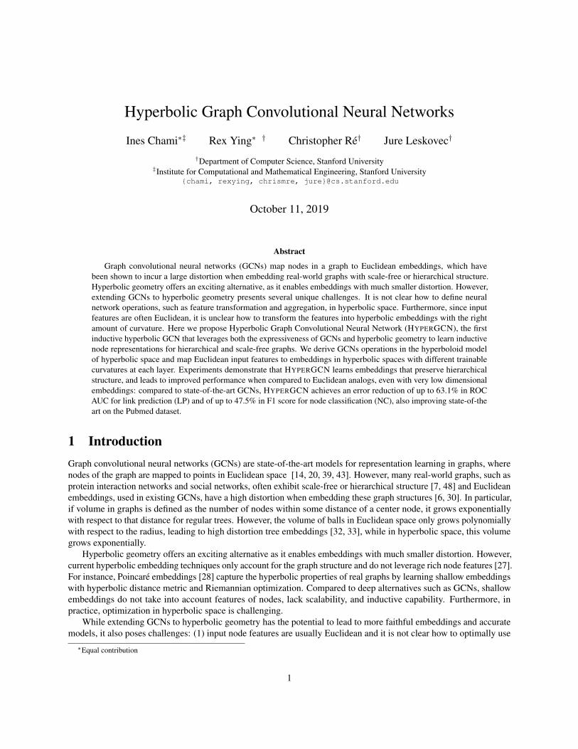
Figure 2: HYPERGCN aggregation (Equation 9)

Geodesics and induced distances. Next, we introduce the notion of geodesics and distances in manifolds, whichare generalizations of shortest paths in graphs or straight lines in Euclidean geometry (Figure 1). Geodesics anddistance functions are particularly important in graph embedding algorithms, as a common optimization objective isminimizing geodesic distances between connected nodes. Let x ∈ Hd,K and u ∈ TxHd,K . Assume u is unit-speed, i.e.〈u,u〉L = 1. We have the following result.

Proposition 3.1. Let x ∈ Hd,K , u ∈ TxHd,K be unit-speed. The unique unit-speed geodesic γx→u(·) such that

γx→u(0) = x, γx→u(0) = u is γKx→u(t) = cosh(

t√K

)x +√Ksinh

(t√K

)u, and the intrinsic distance function

between two points x,y in Hd,K is then

dKL (x,y) =√Karcosh(−〈x,y〉L/K). (4)

Exponential and logarithmic maps. Mapping between tangent space and hyperbolic space is done by the exponentialand logarithmic maps. Given x ∈ Hd,K and a tangent vector v ∈ TxHd,K , the exponential map expKx : TxHd,K →Hd,K is the map that assigns to v the point expKx (v) := γ(1), where γ is the unique geodesic satisfying γ(0) = x andγ(0) = v. The logarithmic map is the reverse map that maps back to the tangent space at x such that logKx (expKx (v)) =v. In general Riemannian manifolds, these operations are only defined locally but in the hyperbolic space, they form abijection between the hyperbolic space and the tangent space at a point. We have the following direct expressions of theexponential and the logarithmic maps which allow us to perform operations on points on the hyperboloid manifold bymapping them to tangent spaces and and vice-versa.

Proposition 3.2. For x ∈ Hd,K , v ∈ TxHd,K and y ∈ Hd,K such that v 6= 0 and y 6= x, the exponential andlogarithmic maps of the hyperboloid model are given by

expKx (v) = cosh(||v||L√K

)x +√Ksinh

(||v||L√K

)v||v||L

, logKx (y) = dKL (x,y)y + 1

K 〈x,y〉Lx||y + 1

K 〈x,y〉Lx||L.

4 Hyperbolic Graph Convolutional NetworksWe introduce HYPERGCN, a generalization of inductive GCNs in hyperbolic geometry that benefits from the ex-pressiveness of both graph neural networks and hyperbolic embeddings. We introduce the essential components ofHYPERGCN. First, since input features are often Euclidean, we derive a mapping from Euclidean features to hyperbolicspace. Next, we derive the two components of graph convolution: The analogs of the Euclidean feature transformationand aggregation (Equations 1, 2) in the hyperboloid model. Finally, we introduce the HYPERGCN algorithm withtrainable curvature.

4

4.1 Mapping from Euclidean to hyperbolic spacesHYPERGCN first maps input features to the hyperboloid manifold via the exp map. Let x0,E ∈ Rd denote inputEuclidean features. For instance, these features could be produced by pre-trained Euclidean neural networks. Leto := {

√K, 0, . . . , 0} ∈ Hd,K denote the north pole (origin) in Hd,K , which we use as a reference point to perform

tangent space operations. We have 〈(0,x0,E),o〉 = 0. Therefore, we interpret (0,x0,E) as a point in ToHd,K and useProposition 3.2 to map it to Hd,K with

x0,H = expKo ((0,x0,E)) =(√

Kcosh(||x0,E ||2√

K

),√Ksinh

(||x0,E ||2√

K

)x0,E

||x0,E ||2

). (5)

4.2 Feature transform in hyperbolic spaceThe feature transform in Equation 1 is used in GCN to map the embedding space of one layer to the next layer embeddingspace and capture large neighborhood structures. We now want to learn transformations of points on the hyperboloidmanifold. However, there is no notion of vector space structure in hyperbolic space. We build upon Hyperbolic NeuralNetwork (HNN) [10] and derive transformations in the hyperboloid model. The main idea is to leverage the exp andlog maps in Corollary 3.2 so that we can use the tangent space ToHd,K to perform Euclidean transformations.

Hyperboloid linear transform. Linear transformation requires a multiplication of the embedding vector by aweight matrix, followed by bias translation. To compute matrix vector multiplication, we first use the log map to projecthyperbolic points xH to ToHd,K . Thus the matrix representing the transform is defined on the tangent space, which isEuclidean and isomorphic to Rd. We then project the vector back to the manifold using the exponential map. Let W bea d′ × d weight matrix, we define the hyperboloid matrix mutiplication as

W ⊗K xH := expKo (W logKo (xH)), (6)

where logKo (·) is on Hd,K and expKo (·) maps to Hd′,K . In order to perform bias addition, we use a result from theHNN model and define b as an Euclidean vector located at ToHd,K . We then parallel transport b to the tangent spaceof the hyperbolic point of interest and map it to the manifold. The hyperboloid bias addition is then defined as

xH ⊕K b := expKxH(PKo→xH (b)), (7)

where PKo→xH (·) is the parallel transport from ToHd′,K to TxHHd′,K (c.f. Appendix A for details).

4.3 Neighborhood aggregation on the hyperboloid manifoldAggregation (Equation 2) is a crucial step in GCNs as it captures neighborhood structures and features with messagepassing. Suppose that xi aggregates information from its neighbors (xj)j∈N (i) with weights (wj)j∈N (i). Meanaggregation in Euclidean GCN computes the weighted average

∑j∈N (i) wjxj . An analog of mean aggregation in

hyperbolic space is the Frechet mean [9], which has no closed form solution. Instead, we propose to perform aggregationin tangent spaces using hyperbolic attention.Attention based aggregation. Attention in GCNs learns a notion of neighbors’ importance, and aggregates neighbors’messages according to their importance to the center node. However, attention on Euclidean embeddings does not takeinto account the nodes’ hierarchies. Thus, we further propose hyperbolic attention-based aggregation. Given hyperbolicembeddings (xHi ,xHj ), we first map xHi and xHj to the tangent space of the origin to compute attention weights wijwith concatenation and Euclidean Multi-layer Percerptron (MLP). We then propose a hyperbolic aggregation to averagenodes’ representations

wij = SOFTMAXj∈N (i)(MLP(logKo (xHi )||logKo (xHj ))) (8)

AGGK(xH)i = expKxHi

( ∑j∈N (i)

wij logKxHi

(xHj )). (9)

Note that our proposed aggregation is directly performed in the tangent space of each center point xHi , as this is wherethe Euclidean approximation is best (cf. Figure 2). We show in our ablation experiments (cf. Table 2) that this local

5

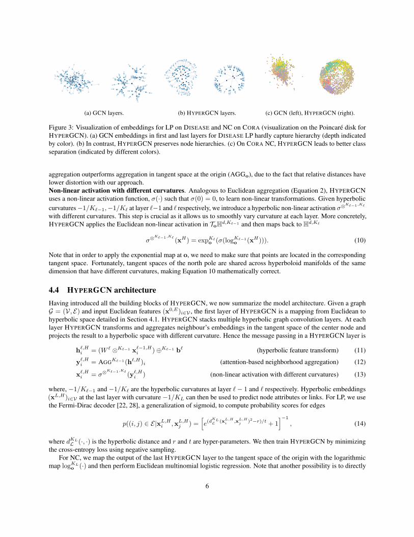
(a) GCN layers. (b) HYPERGCN layers. (c) GCN (left), HYPERGCN (right).

Figure 3: Visualization of embeddings for LP on DISEASE and NC on CORA (visualization on the Poincaré disk forHYPERGCN). (a) GCN embeddings in first and last layers for DISEASE LP hardly capture hierarchy (depth indicatedby color). (b) In contrast, HYPERGCN preserves node hierarchies. (c) On CORA NC, HYPERGCN leads to better classseparation (indicated by different colors).

aggregation outperforms aggregation in tangent space at the origin (AGGo), due to the fact that relative distances havelower distortion with our approach.Non-linear activation with different curvatures. Analogous to Euclidean aggregation (Equation 2), HYPERGCNuses a non-linear activation function, σ(·) such that σ(0) = 0, to learn non-linear transformations. Given hyperboliccurvatures−1/K`−1,−1/K` at layer `−1 and ` respectively, we introduce a hyperbolic non-linear activation σ⊗

K`−1,K`

with different curvatures. This step is crucial as it allows us to smoothly vary curvature at each layer. More concretely,HYPERGCN applies the Euclidean non-linear activation in ToHd,K`−1 and then maps back to Hd,K`

σ⊗K`−1,K` (xH) = expK`

o (σ(logK`−1o (xH))). (10)

Note that in order to apply the exponential map at o, we need to make sure that points are located in the correspondingtangent space. Fortunately, tangent spaces of the north pole are shared across hyperboloid manifolds of the samedimension that have different curvatures, making Equation 10 mathematically correct.

4.4 HYPERGCN architectureHaving introduced all the building blocks of HYPERGCN, we now summarize the model architecture. Given a graphG = (V, E) and input Euclidean features (x0,E)i∈V , the first layer of HYPERGCN is a mapping from Euclidean tohyperbolic space detailed in Section 4.1. HYPERGCN stacks multiple hyperbolic graph convolution layers. At eachlayer HYPERGCN transforms and aggregates neighbour’s embeddings in the tangent space of the center node andprojects the result to a hyperbolic space with different curvature. Hence the message passing in a HYPERGCN layer is

h`,Hi = (W ` ⊗K`−1 x`−1,Hi )⊕K`−1 b` (hyperbolic feature transform) (11)

y`,Hi = AGGK`−1(h`,H)i (attention-based neighborhood aggregation) (12)

x`,Hi = σ⊗K`−1,K` (y`,Hi ) (non-linear activation with different curvatures) (13)

where, −1/K`−1 and −1/K` are the hyperbolic curvatures at layer `− 1 and ` respectively. Hyperbolic embeddings(xL,H)i∈V at the last layer with curvature −1/KL can then be used to predict node attributes or links. For LP, we usethe Fermi-Dirac decoder [22, 28], a generalization of sigmoid, to compute probability scores for edges

p((i, j) ∈ E|xL,Hi ,xL,Hj ) =[e(dKLL (xL,H

i,xL,H

j)2−r)/t + 1

]−1, (14)

where dKL

L (·, ·) is the hyperbolic distance and r and t are hyper-parameters. We then train HYPERGCN by minimizingthe cross-entropy loss using negative sampling.

For NC, we map the output of the last HYPERGCN layer to the tangent space of the origin with the logarithmicmap logKL

o (·) and then perform Euclidean multinomial logistic regression. Note that another possibility is to directly

6

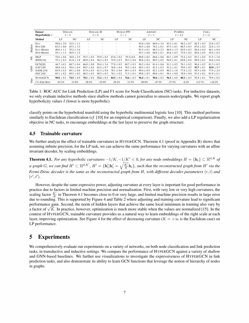
Dataset DISEASE DISEASE-M HUMAN PPI AIRPORT PUBMED CORAHyperbolicity δ δ = 0 δ = 0 δ = 1 δ = 1 δ = 3.5 δ = 11Method LP NC LP NC LP NC LP NC LP NC LP NC

Shal

low

EUC 59.8 ± 2.0 32.5 ± 1.1 - - - - 92.0 ± 0.0 60.9 ± 3.4 83.3 ± 0.1 48.2 ± 0.7 82.5 ± 0.3 23.8 ± 0.7HYP [28] 63.5 ± 0.6 45.5 ± 3.3 - - - - 94.5 ± 0.0 70.2 ± 0.1 87.5 ± 0.1 68.5 ± 0.3 87.6 ± 0.2 22.0 ± 1.5EUC-MIXED 49.6 ± 1.1 35.2 ± 3.4 - - - - 91.5 ± 0.1 68.3 ± 2.3 86.0 ± 1.3 63.0 ± 0.3 84.4 ± 0.2 46.1 ± 0.4HYP-MIXED 55.1 ± 1.3 56.9 ± 1.5 - - - - 93.3 ± 0.0 69.6 ± 0.1 83.8 ± 0.3 73.9 ± 0.2 85.6 ± 0.5 45.9 ± 0.3

NN MLP 72.6 ± 0.6 28.8 ± 2.5 55.3 ± 0.5 55.9 ± 0.3 67.8 ± 0.2 55.3±0.4 89.8 ± 0.5 68.6 ± 0.6 84.1 ± 0.9 72.4 ± 0.2 83.1 ± 0.5 51.5 ± 1.0

HNN[10] 75.1 ± 0.3 41.0 ± 1.8 60.9 ± 0.4 56.2 ± 0.3 72.9 ± 0.3 59.3 ± 0.4 90.8 ± 0.2 80.5 ± 0.5 94.9 ± 0.1 69.8 ± 0.4 89.0 ± 0.1 54.6 ± 0.4

GN

N

GCN[20] 64.7 ±0.5 69.7 ± 0.4 66.0 ± 0.8 59.4 ± 3.4 77.0 ± 0.5 69.7 ± 0.3 89.3 ± 0.4 81.4 ± 0.6 91.1 ± 0.5 78.1 ± 0.2 90.4 ± 0.2 81.3 ± 0.3GAT [39] 69.8 ±0.3 70.4 ± 0.4 69.5 ± 0.4 62.5 ± 0.7 76.8 ± 0.4 70.5 ± 0.4 90.5 ± 0.3 81.5 ± 0.3 91.2 ± 0.1 79.0 ± 0.3 93.7 ± 0.1 83.0 ± 0.7SAGE [14] 65.9 ± 0.3 69.1 ± 0.6 67.4 ± 0.5 61.3 ± 0.4 78.1 ± 0.6 69.1 ± 0.3 90.4 ± 0.5 82.1 ± 0.5 86.2 ± 1.0 77.4 ± 2.2 85.5 ± 0.6 77.9 ± 2.4SGC [42] 65.1 ± 0.2 69.5 ± 0.2 66.2 ± 0.2 60.5 ± 0.3 76.1 ± 0.2 71.3 ± 0.1 89.8 ± 0.3 80.6 ± 0.1 94.1 ± 0.0 78.9 ± 0.0 91.5 ± 0.1 81.0 ± 0.1

Our

s HYPERGCN 90.8 ± 0.3 74.5 ± 0.9 78.1 ± 0.4 72.2 ± 0.5 84.5 ± 0.4 74.6 ± 0.3 96.4 ± 0.1 90.6 ± 0.2 96.3 ± 0.0 80.3 ± 0.3 92.9 ± 0.1 79.9 ± 0.2

(%) ERR RED -63.1% -13.8% -28.2% -25.9% -29.2% -11.5% -60.9% -47.5% -27.5% -6.2% +12.7% +18.2%

Table 1: ROC AUC for Link Prediction (LP) and F1 score for Node Classification (NC) tasks. For inductive datasets,we only evaluate inductive methods since shallow methods cannot generalize to unseen nodes/graphs. We report graphhyperbolicity values δ (lower is more hyperbolic).

classify points on the hyperboloid manifold using the hyperbolic multinomial logistic loss [10]. This method performssimilarly to Euclidean classification (cf. [10] for an empirical comparison). Finally, we also add a LP regularizationobjective in NC tasks, to encourage embeddings at the last layer to preserve the graph structure.

4.5 Trainable curvatureWe further analyze the effect of trainable curvatures in HYPERGCN. Theorem 4.1 (proof in Appendix B) shows thatassuming infinite precision, for the LP task, we can achieve the same performance for varying curvatures with an affineinvariant decoder, by scaling embeddings.

Theorem 4.1. For any hyperbolic curvatures −1/K,−1/K ′ < 0, for any node embeddings H = {hi} ⊂ Hd,K of

a graph G, we can find H ′ ⊂ Hd,K′ , H ′ = {h′i|h′i =√

K′

K hi}, such that the reconstructed graph from H ′ via theFermi-Dirac decoder is the same as the reconstructed graph from H , with different decoder parameters (r, t) and(r′, t′).

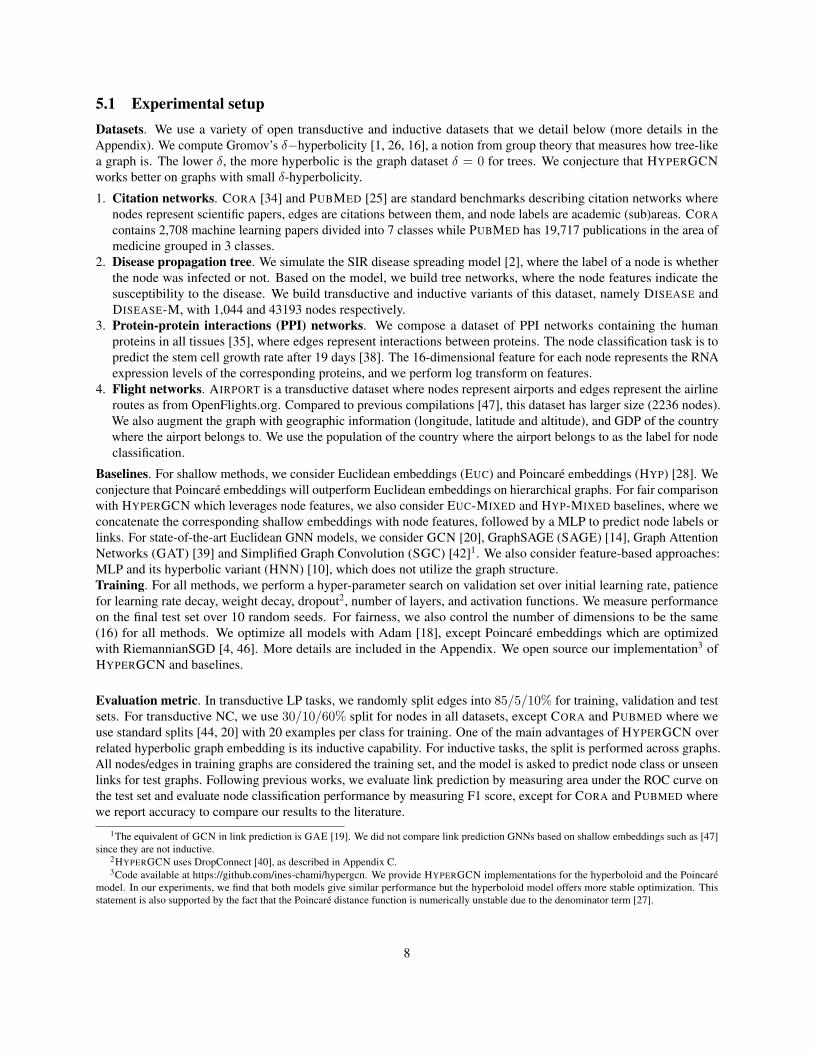
However, despite the same expressive power, adjusting curvature at every layer is important for good performance inpractice due to factors in limited machine precision and normalization. First, with very low or very high curvatures, thescaling factor K

′

K in Theorem 4.1 becomes close to 0 or very large, and limited machine precision results in large errordue to rounding. This is supported by Figure 4 and Table 2 where adjusting and training curvature lead to significantperformance gain. Second, the norm of hidden layers that achieve the same local minimum in training also vary bya factor of

√K. In practice, however, optimization is much more stable when the values are normalized [15]. In the

context of HYPERGCN, trainable curvature provides us a natural way to learn embeddings of the right scale at eachlayer, improving optimization. See Figure 4 for the effect of decreasing curvature (K = +∞ is the Euclidean case) onLP performance.

5 ExperimentsWe comprehensively evaluate our experiments on a variety of networks, on both node classification and link predictiontasks, in transductive and inductive settings. We compare the performance of HYPERGCN against a variety of shallowand GNN-based baselines. We further use visualizations to investigate the expressiveness of HYPERGCN in linkprediction tasks, and also demonstrate its ability to learn GCN functions that leverage the notion of hierarchy of nodesin graphs.

7

5.1 Experimental setupDatasets. We use a variety of open transductive and inductive datasets that we detail below (more details in theAppendix). We compute Gromov’s δ−hyperbolicity [1, 26, 16], a notion from group theory that measures how tree-likea graph is. The lower δ, the more hyperbolic is the graph dataset δ = 0 for trees. We conjecture that HYPERGCNworks better on graphs with small δ-hyperbolicity.

1. Citation networks. CORA [34] and PUBMED [25] are standard benchmarks describing citation networks wherenodes represent scientific papers, edges are citations between them, and node labels are academic (sub)areas. CORAcontains 2,708 machine learning papers divided into 7 classes while PUBMED has 19,717 publications in the area ofmedicine grouped in 3 classes.

2. Disease propagation tree. We simulate the SIR disease spreading model [2], where the label of a node is whetherthe node was infected or not. Based on the model, we build tree networks, where the node features indicate thesusceptibility to the disease. We build transductive and inductive variants of this dataset, namely DISEASE andDISEASE-M, with 1,044 and 43193 nodes respectively.

3. Protein-protein interactions (PPI) networks. We compose a dataset of PPI networks containing the humanproteins in all tissues [35], where edges represent interactions between proteins. The node classification task is topredict the stem cell growth rate after 19 days [38]. The 16-dimensional feature for each node represents the RNAexpression levels of the corresponding proteins, and we perform log transform on features.

4. Flight networks. AIRPORT is a transductive dataset where nodes represent airports and edges represent the airlineroutes as from OpenFlights.org. Compared to previous compilations [47], this dataset has larger size (2236 nodes).We also augment the graph with geographic information (longitude, latitude and altitude), and GDP of the countrywhere the airport belongs to. We use the population of the country where the airport belongs to as the label for nodeclassification.

Baselines. For shallow methods, we consider Euclidean embeddings (EUC) and Poincaré embeddings (HYP) [28]. Weconjecture that Poincaré embeddings will outperform Euclidean embeddings on hierarchical graphs. For fair comparisonwith HYPERGCN which leverages node features, we also consider EUC-MIXED and HYP-MIXED baselines, where weconcatenate the corresponding shallow embeddings with node features, followed by a MLP to predict node labels orlinks. For state-of-the-art Euclidean GNN models, we consider GCN [20], GraphSAGE (SAGE) [14], Graph AttentionNetworks (GAT) [39] and Simplified Graph Convolution (SGC) [42]1. We also consider feature-based approaches:MLP and its hyperbolic variant (HNN) [10], which does not utilize the graph structure.Training. For all methods, we perform a hyper-parameter search on validation set over initial learning rate, patiencefor learning rate decay, weight decay, dropout2, number of layers, and activation functions. We measure performanceon the final test set over 10 random seeds. For fairness, we also control the number of dimensions to be the same(16) for all methods. We optimize all models with Adam [18], except Poincaré embeddings which are optimizedwith RiemannianSGD [4, 46]. More details are included in the Appendix. We open source our implementation3 ofHYPERGCN and baselines.

Evaluation metric. In transductive LP tasks, we randomly split edges into 85/5/10% for training, validation and testsets. For transductive NC, we use 30/10/60% split for nodes in all datasets, except CORA and PUBMED where weuse standard splits [44, 20] with 20 examples per class for training. One of the main advantages of HYPERGCN overrelated hyperbolic graph embedding is its inductive capability. For inductive tasks, the split is performed across graphs.All nodes/edges in training graphs are considered the training set, and the model is asked to predict node class or unseenlinks for test graphs. Following previous works, we evaluate link prediction by measuring area under the ROC curve onthe test set and evaluate node classification performance by measuring F1 score, except for CORA and PUBMED wherewe report accuracy to compare our results to the literature.

1The equivalent of GCN in link prediction is GAE [19]. We did not compare link prediction GNNs based on shallow embeddings such as [47]since they are not inductive.

2HYPERGCN uses DropConnect [40], as described in Appendix C.3Code available at https://github.com/ines-chami/hypergcn. We provide HYPERGCN implementations for the hyperboloid and the Poincaré

model. In our experiments, we find that both models give similar performance but the hyperboloid model offers more stable optimization. Thisstatement is also supported by the fact that the Poincaré distance function is numerically unstable due to the denominator term [27].

8

−3 −2 −1 0 1−log(K)

0.5

0.6

0.7

0.8

0.9

RO

CA

UC

Figure 4: Decreasing curvature (−1/K) improves linkprediction performance on DISEASE.

Method DISEASE AIRPORT

HYPERGCN 78.4 ± 0.3 91.8 ± 0.3HYPERGCN-ATTo 80.9 ± 0.4 92.3 ± 0.3HYPERGCN-ATT 82.0 ± 0.2 92.5 ± 0.2

HYPERGCN-C 89.1 ± 0.2 94.9 ± 0.3HYPERGCN-ATT-C 90.8 ± 0.3 96.4 ± 0.1

Table 2: ROC AUC for link prediction on AIRPORT andDISEASE datasets.

5.2 ResultsTable 1 reports the performance of HYPERGCN in comparison to baseline methods. HYPERGCN works best ininductive scenarios where both node features and network topology play an important role. The performance gain ofHYPERGCN with respect to Euclidean GNN models is correlated with graph hyperbolicity. HYPERGCN achievesan average of 45.4% (LP) and 12.3% (NC) error reduction compared with the best deep baselines for graphs withhigh hyperbolicity (low δ), suggesting that GNNs can significantly benefit from hyperbolic geometry, especially inlink prediction tasks. Furthermore, the performance gap between HYPERGCN and HNN suggests that neighborhoodaggregation has been effective in learning node representations in graphs. For example, in disease spread datasets, bothEuclidean attention and hyperbolic geometry lead to significant improvement of HYPERGCN over other baselines.This can be explained by the fact that in disease spread trees, parent nodes contaminate their children. HYPERGCN cansuccessfully model these asymmetric and hierarchical relationships with hyperbolic attention and improves performanceover all baselines.

On the CORA dataset with low hyperbolicity, HYPERGCN does not outperform Euclidean GNNs, suggestingthat Euclidean geometry is better for its underlying graph structure. However, for small dimensions, HYPERGCN isstill significantly more effective than GCN even with CORA. Figure 3c shows 2-dimensional HYPERGCN and GCNembeddings trained with LP objective, where colors denote the label class. HYPERGCN achieves much better labelclass separation.

5.3 AnalysisAblations. We further analyze the effect of proposed components in HYPERGCN, namely hyperbolic attention (ATT)and trainable curvature (C) on AIRPORT and DISEASE datasets in Table 2. We observe that both attention and trainablecurvature lead to performance gains over HYPERGCN with fixed curvature and no attention. Furthermore, our attentionmodel ATT outperforms ATTo (aggregation in tangent space at o) and we conjecture that this is because the localEuclidean average is a better approximation near the center point rather than near o. Finally, the addition of both ATTand C improves performance even further, suggesting that both components are important in the HYPERGCN model.Visualizations. We first visualize the GCN and HYPERGCN embeddings at the first and last layers in Figure 3. Wetrain HYPERGCN with 3-dimensional hyperbolic embeddings and map them to the Poincaré disk which is better forvisualization. In contrast to GCN, the tree structure is preserved in HYPERGCN, where nodes close to the center areof higher hierarchy in the tree. HYPERGCN smoothly transforms Euclidean features to Hyperbolic embeddings thatpreserve node hierarchies.

Figure 5 shows the attention weights in the 2-hop neighborhood of a center node (red) for the DISEASE dataset. Thered node is the node where we compute attention. The darkness of the color for other nodes denotes their hierarchy.The attention weights for nodes in the neighborhood are visualized by the intensity of edges. We observe that inHYPERGCN the center node pays more attention to its (grand)parent. In contrast to Euclidean GAT, our aggregationwith attention in hyperbolic space allows us to pay more attention to nodes with high hierarchy. Such attention is crucialto good performance in DISEASE, because only sick parents will propagate the disease to their children.

9

Figure 5: Attention: Euclidean GAT (left), HYPERGCN (right). Each graph represents a 2-hop neighborhood of theDISEASE-M dataset.

6 ConclusionWe introduced HYPERGCN, a novel architecture that learns hyperbolic embeddings using graph convolutional networks.In HYPERGCN, the Euclidean input features are successively mapped to embeddings in hyperbolic spaces with trainablecurvatures at every layer. HYPERGCN achieves new state-of-the-art in learning embeddings for real-world hierarchicaland scale-free graphs.

Acknowledgments

Jure Leskovec is a Chan Zuckerberg Biohub investigator. This research has been supported in part by NSF OAC-1835598,DARPA MCS, DARPA ASED, ARO MURI, Boeing, Docomo, Hitachi, Huawei, JD, Siemens and Stanford Data ScienceInitiative. We gratefully acknowledge the support of DARPA under Nos. FA87501720095 (D3M), FA86501827865(SDH), and FA86501827882 (ASED); NIH under No. U54EB020405 (Mobilize), NSF under Nos. CCF1763315(Beyond Sparsity), CCF1563078 (Volume to Velocity), and 1937301 (RTML); ONR under No. N000141712266(Unifying Weak Supervision); the Moore Foundation, NXP, Xilinx, LETI-CEA, Intel, Microsoft, NEC, Toshiba, TSMC,ARM, Hitachi, BASF, Accenture, Ericsson, Qualcomm, Analog Devices, the Okawa Foundation, American FamilyInsurance, Google Cloud, Swiss Re, and members of the Stanford DAWN project: Teradata, Facebook, Google, AntFinancial, NEC, VMWare, and Infosys. The U.S. Government is authorized to reproduce and distribute reprints forGovernmental purposes notwithstanding any copyright notation thereon. Any opinions, findings, and conclusions orrecommendations expressed in this material are those of the authors and do not necessarily reflect the views, policies, orendorsements, either expressed or implied, of DARPA, NIH, ONR, or the U.S. Government.

References[1] Aaron B Adcock, Blair D Sullivan, and Michael W Mahoney. Tree-like structure in large social and information

networks. In 2013 IEEE 13th International Conference on Data Mining, pages 1–10. IEEE, 2013.

[2] Roy M Anderson and Robert M May. Infectious diseases of humans: dynamics and control. Oxford universitypress, 1992.

[3] Mikhail Belkin and Partha Niyogi. Laplacian eigenmaps and spectral techniques for embedding and clustering. InAdvances in neural information processing systems, pages 585–591, 2002.

[4] Silvere Bonnabel. Stochastic gradient descent on riemannian manifolds. IEEE Transactions on Automatic Control,2013.

[5] Benjamin Paul Chamberlain, James Clough, and Marc Peter Deisenroth. Neural embeddings of graphs inhyperbolic space. arXiv preprint arXiv:1705.10359, 2017.

[6] Wei Chen, Wenjie Fang, Guangda Hu, and Michael W Mahoney. On the hyperbolicity of small-world and treelikerandom graphs. Internet Mathematics, 9(4):434–491, 2013.

10

[7] Aaron Clauset, Cristopher Moore, and Mark EJ Newman. Hierarchical structure and the prediction of missinglinks in networks. Nature, 453(7191):98, 2008.

[8] Bhuwan Dhingra, Christopher J Shallue, Mohammad Norouzi, Andrew M Dai, and George E Dahl. Embeddingtext in hyperbolic spaces. NAACL HLT, 2018.

[9] Maurice Fréchet. Les éléments aléatoires de nature quelconque dans un espace distancié. In Annales de l’institutHenri Poincaré, 1948.

[10] Octavian Ganea, Gary Bécigneul, and Thomas Hofmann. Hyperbolic neural networks. In NeurIPS, 2018.

[11] Octavian-Eugen Ganea, Gary Bécigneul, and Thomas Hofmann. Hyperbolic entailment cones for learninghierarchical embeddings. In International Conference on Machine Learning ICML, 2018.

[12] Aditya Grover and Jure Leskovec. node2vec: Scalable feature learning for networks. In KDD, 2016.

[13] Caglar Gulcehre, Misha Denil, Mateusz Malinowski, Ali Razavi, Razvan Pascanu, Karl Moritz Hermann, PeterBattaglia, Victor Bapst, David Raposo, Adam Santoro, et al. Hyperbolic attention networks. In ICLR, 2019.

[14] Will Hamilton, Zhitao Ying, and Jure Leskovec. Inductive representation learning on large graphs. In NIPS, 2017.

[15] Sergey Ioffe and Christian Szegedy. Batch normalization: Accelerating deep network training by reducing internalcovariate shift. In ICML, 2015.

[16] Edmond Jonckheere, Poonsuk Lohsoonthorn, and Francis Bonahon. Scaled gromov hyperbolic graphs. Journal ofGraph Theory, 2008.

[17] Valentin Khrulkov, Leyla Mirvakhabova, Evgeniya Ustinova, Ivan Oseledets, and Victor Lempitsky. Hyperbolicimage embeddings. arXiv preprint arXiv:1904.02239, 2019.

[18] Diederik P Kingma and Jimmy Ba. Adam: A method for stochastic optimization. In ICLR, 2015.

[19] Thomas N Kipf and Max Welling. Variational graph auto-encoders. NIPS Workshop on Bayesian Deep Learning,2016.

[20] Thomas N Kipf and Max Welling. Semi-supervised classification with graph convolutional networks. In ICLR,2017.

[21] Robert Kleinberg. Geographic routing using hyperbolic space. In IEEE International Conference on ComputerCommunications, 2007.

[22] Dmitri Krioukov, Fragkiskos Papadopoulos, Maksim Kitsak, Amin Vahdat, and Marián Boguná. Hyperbolicgeometry of complex networks. Physical Review E, 2010.

[23] Joseph B Kruskal. Multidimensional scaling by optimizing goodness of fit to a nonmetric hypothesis. Psychome-trika, 1964.

[24] Yujia Li, Daniel Tarlow, Marc Brockschmidt, and Richard Zemel. Gated graph sequence neural networks. InICLR, 2016.

[25] Galileo Namata, Ben London, Lise Getoor, Bert Huang, and UMD EDU. Query-driven active surveying forcollective classification. 2012.

[26] Onuttom Narayan and Iraj Saniee. Large-scale curvature of networks. Physical Review E, 84(6):066108, 2011.

[27] Maximilian Nickel and Douwe Kiela. Learning continuous hierarchies in the lorentz model of hyperbolic geometry.ICML, 2018.

11

[28] Maximillian Nickel and Douwe Kiela. Poincaré embeddings for learning hierarchical representations. In NIPS,2017.

[29] Bryan Perozzi, Rami Al-Rfou, and Steven Skiena. Deepwalk: Online learning of social representations. InProceedings of the 20th ACM SIGKDD international conference on Knowledge discovery and data mining, pages701–710. ACM, 2014.

[30] Erzsébet Ravasz and Albert-László Barabási. Hierarchical organization in complex networks. Physical review E,2003.

[31] Joel W Robbin and Dietmar A Salamon. Introduction to differential geometry.

[32] Frederic Sala, Chris De Sa, Albert Gu, and Christopher Re. Representation tradeoffs for hyperbolic embeddings.In ICML, 2018.

[33] Rik Sarkar. Low distortion delaunay embedding of trees in hyperbolic plane. In International Symposium onGraph Drawing, 2011.

[34] Prithviraj Sen, Galileo Namata, Mustafa Bilgic, Lise Getoor, Brian Galligher, and Tina Eliassi-Rad. Collectiveclassification in network data. AI magazine, 2008.

[35] Damian Szklarczyk, John H Morris, Helen Cook, Michael Kuhn, Stefan Wyder, Milan Simonovic, AlbertoSantos, Nadezhda T Doncheva, Alexander Roth, Peer Bork, et al. The string database in 2017: quality-controlledprotein–protein association networks, made broadly accessible. Nucleic acids research, 2016.

[36] Yi Tay, Luu Anh Tuan, and Siu Cheung Hui. Hyperbolic representation learning for fast and efficient neuralquestion answering. In WSDM, 2018.

[37] Alexandru Tifrea, Gary Becigneul, and Octavian-Eugen Ganea. Poincaré glove: Hyperbolic word embeddings. InICLR, 2019.

[38] Joyce van de Leemput, Nathan C Boles, Thomas R Kiehl, Barbara Corneo, Patty Lederman, Vilas Menon,Changkyu Lee, Refugio A Martinez, Boaz P Levi, Carol L Thompson, et al. Cortecon: a temporal transcriptomeanalysis of in vitro human cerebral cortex development from human embryonic stem cells. Neuron, 2014.

[39] Petar Velickovic, Guillem Cucurull, Arantxa Casanova, Adriana Romero, Pietro Lio, and Yoshua Bengio. Graphattention networks. ICLR, 2018.

[40] Li Wan, Matthew Zeiler, Sixin Zhang, Yann Le Cun, and Rob Fergus. Regularization of neural networks usingdropconnect. In ICML, 2013.

[41] Richard C Wilson, Edwin R Hancock, Elzbieta Pekalska, and Robert PW Duin. Spherical and hyperbolicembeddings of data. IEEE transactions on pattern analysis and machine intelligence, 36(11):2255–2269, 2014.

[42] Felix Wu, Tianyi Zhang, Amauri Holanda de Souza Jr, Christopher Fifty, Tao Yu, and Kilian Q Weinberger.Simplifying graph convolutional networks. In ICML, 2019.

[43] Keyulu Xu, Weihua Hu, Jure Leskovec, and Stefanie Jegelka. How powerful are graph neural networks? ICLR,2019.

[44] Zhilin Yang, William W Cohen, and Ruslan Salakhutdinov. Revisiting semi-supervised learning with graphembeddings. ICML, 2016.

[45] Rex Ying, Ruining He, Kaifeng Chen, Pong Eksombatchai, William L Hamilton, and Jure Leskovec. Graphconvolutional neural networks for web-scale recommender systems. In KDD, 2018.

[46] Hongyi Zhang, Sashank J Reddi, and Suvrit Sra. Riemannian svrg: Fast stochastic optimization on riemannianmanifolds. In NIPS, 2016.

12

[47] Muhan Zhang and Yixin Chen. Link prediction based on graph neural networks. In NeurIPS, 2018.

[48] Marinka Zitnik, Rok Sosic, Marcus W. Feldman, and Jure Leskovec. Evolution of resilience in protein interactomesacross the tree of life. Proceedings of the National Academy of Sciences.

13

A Review of Differential GeometryWe first recall some definitions of differential and hyperbolic geometry.

A.1 Differential geometryManifold. An d−dimensional manifold M is a topological space that locally resembles the topological space Rdnear each point. More concretely, for each point x onM, we can find a homeomorphism (continuous bijection withcontinuous inverse) between a neighbourhood of x and Rd. The notion of manifold is a generalization of surfaces inhigh dimensions.Tangent space. Intuitively, if we think ofM as a d−dimensional manifold embedded in Rd+1, the tangent spaceTxM at point x onM is a d−dimensional hyperplane in Rd+1 that best approximatesM around x. Another possibleinterpretation for TxM is that it contains all the possible directions of curves onM passing through x. The elements ofTxM are called tangent vectors and the union of all tangent spaces is called the tangent bundle TM = ∪x∈MTxM.Riemannian manifold. A Riemannian manifold is a pair (M,g), whereM is a smooth manifold and g = (gx)x∈Mis a Riemannian metric, that is a family of smoothly varying inner products on tangent spaces, gx : TxM×TxM→ R.Riemannian metrics can be used to measure distances on manifolds.Distances and geodesics. Let (M,g) be a Riemannian manifold. For v ∈ TxM, define the norm of v by ||v||g :=√gx(v,v). Suppose γ : [a, b]→M is a smooth curve onM. Define the length of γ by

L(γ) :=∫ b

a

||γ′(t)||gdt.

Now with this definition of length, every connected Riemannian manifold becomes a metric space and the distanced :M×M→ [0,∞) is defined as

d(x,y) := infγ{L(γ) : γ is a continuously differentiable curve joining x and y}.

Geodesic distances are a generalization of straight lines (or shortest paths) to non-Euclidean geometry. A curveγ : [a, b]→M is geodesic if d(γ(t), γ(s)) = L(γ|[t,s])∀(t, s) ∈ [a, b](t < s).Parallel transport. Parallel transport is a generalization of translation to non-Euclidean geometry. Given a smoothmanifoldM, parallel transport Px→y(·) maps a vector v ∈ TxM to Px→y(v) ∈ TyM. In Riemannian geometry,parallel transport preserves the Riemannian metric tensor (norm, inner products...).Curvature. At a high level, curvature measures how much a geometric object such as surfaces deviate from a flat plane.For instance, the Euclidean space has zero curvature while spheres have positive curvature. We illustrate the concept ofcurvature in Figure 6.

A.2 Hyperbolic geometryHyperbolic space. The hyperbolic space in d dimensions is the unique complete, simply connected d−dimensionalRiemannian manifold with constant negative sectional curvature. There exist several models of hyperbolic space suchas the Poincaré model or the hyperboloid model (also known as the Minkowski model or the Lorentz model). In whatfollows, we review the Poincaré and the hyperboloid models of hyperbolic space as well as connections between thesetwo models.

A.2.1 Poincaré ball model

Let ||.||2 be the Euclidean norm. The Poincaré ball model with unit radius and constant negative curvature −1 in ddimensions is the Riemannian manifold (Dd,1, (gx)x) where

Dd,1 := {x ∈ Rd : ||x||2 < 1},

andgx = λ2

xId,

14

Figure 6: From left to right: a surface of negative curvature, a surface of zero curvature, and a surface of positivecurvature.

where λx := 21−||x||22

and Id is the identity matrix. The induced distance between two points (x,y) in Dd,1 can becomputed as

d1D(x,y) = arcosh

(1 + 2 ||x− y||22

(1− ||x||22)(1− ||y||22)

).

A.2.2 Hyperboloid model

Hyperboloid model. Let 〈., .〉L : Rd+1 × Rd+1 → R denote the Minkowski inner product,

〈x,y〉L := −x0y0 + x1y1 + . . .+ xdyd.

The hyperboloid model with unit imaginary radius and constant negative curvature −1 in d dimensions is defined as theRiemannian manifold (Hd,1, (gx)x) where

Hd,1 := {x ∈ Rd+1 : 〈x,x〉L = −1, x0 > 0},

and

gx :=

−1

1. . .

1

.

The induced distance between two points (x,y) in Hd,1 can be computed as

d1L(x,y) = arcosh(−〈x,y〉L).

Geodesics. We recall a result that gives the unit speed geodesics in the hyperboloid model with curvature −1 [31]. Thisresult allow us to derive Corollary 3.1 and 3.2 for the hyperboloid manifold with negative curvature −1/K, and thenlearn K as a model parameter in HYPERGCN.

Theorem A.1. Let x ∈ Hd,1 and u ∈ TxHd,1 unit-speed (i.e. 〈u,u〉L = 1). The unique unit-speed geodesicγx→u : [0, 1]→ Hd,1 such that γx→u(0) = x and γx→u(0) = u is given by

γx→u(t) = cosh(t)x + sinh(t)u.

15

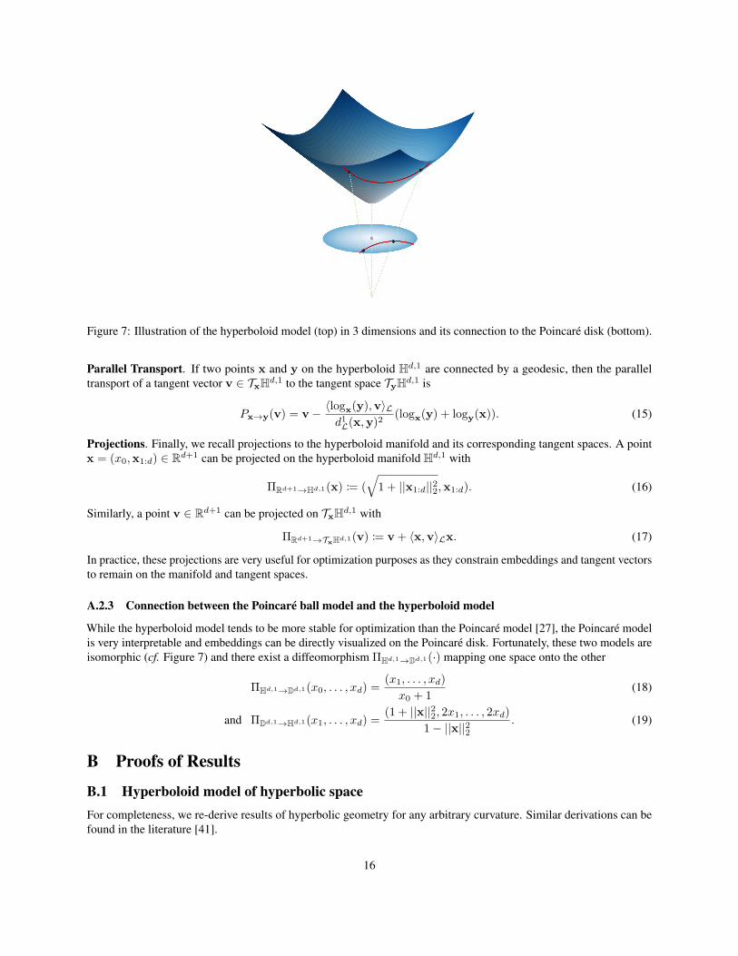
Figure 7: Illustration of the hyperboloid model (top) in 3 dimensions and its connection to the Poincaré disk (bottom).

Parallel Transport. If two points x and y on the hyperboloid Hd,1 are connected by a geodesic, then the paralleltransport of a tangent vector v ∈ TxHd,1 to the tangent space TyHd,1 is

Px→y(v) = v− 〈logx(y),v〉Ld1L(x,y)2 (logx(y) + logy(x)). (15)

Projections. Finally, we recall projections to the hyperboloid manifold and its corresponding tangent spaces. A pointx = (x0,x1:d) ∈ Rd+1 can be projected on the hyperboloid manifold Hd,1 with

ΠRd+1→Hd,1(x) := (√

1 + ||x1:d||22,x1:d). (16)

Similarly, a point v ∈ Rd+1 can be projected on TxHd,1 with

ΠRd+1→TxHd,1(v) := v + 〈x,v〉Lx. (17)

In practice, these projections are very useful for optimization purposes as they constrain embeddings and tangent vectorsto remain on the manifold and tangent spaces.

A.2.3 Connection between the Poincaré ball model and the hyperboloid model

While the hyperboloid model tends to be more stable for optimization than the Poincaré model [27], the Poincaré modelis very interpretable and embeddings can be directly visualized on the Poincaré disk. Fortunately, these two models areisomorphic (cf. Figure 7) and there exist a diffeomorphism ΠHd,1→Dd,1(·) mapping one space onto the other

ΠHd,1→Dd,1(x0, . . . , xd) = (x1, . . . , xd)x0 + 1 (18)

and ΠDd,1→Hd,1(x1, . . . , xd) = (1 + ||x||22, 2x1, . . . , 2xd)1− ||x||22

. (19)

B Proofs of Results

B.1 Hyperboloid model of hyperbolic spaceFor completeness, we re-derive results of hyperbolic geometry for any arbitrary curvature. Similar derivations can befound in the literature [41].

16

Proposition 3.1. Let x ∈ Hd,K , u ∈ TxHd,K be unit-speed. The unique unit-speed geodesic γx→u(·) such that

γx→u(0) = x, γx→u(0) = u is γKx→u(t) = cosh(

t√K

)x +√Ksinh

(t√K

)u, and the intrinsic distance function

between two points x,y in Hd,K is then

dKL (x,y) =√Karcosh(−〈x,y〉L/K). (4)

Proof. We know that the unique unit-speed geodesic γKx→u(.) in Hd,K must satisfy

γKx→u(0) = x and γKx→u(0) = u andd

dt〈γKx→u(t), γKx→u(t)〉L = 0 ∀t. (20)

Let γKx→u(t) = cosh( t√K

)x +√Ksinh( t√

K)u. We have γKx→u(0) = x and γKx→u(0) = u. Furthermore, since

u ∈ TxHd,K , we have 〈u,x〉L = 0 and for all t:

〈γKx→u(t), γKx→u(t)〉L = cosh2( t√K

)〈x,x〉L +Ksinh2( t√K

)〈u,u〉L

= −Kcosh2( t√K

) +Ksinh2( t√K

)

= −K.

Therefore, γKx→u(·) is a curve on Hd,K . Furthermore, we have γKx→u(t) = 1√K

sinh( t√K

)x+cosh( t√K

)u and therefore

d

dt〈γKx→u(t), γKx→u(t)〉L = d

dt( 1K

sinh2( t√K

)〈x,x〉L + cosh2( t√K

)〈u,u〉L)

= d

dt(−sinh2( t√

K) + cosh2( t√

K))

= 0.

Finally, γKx→u(.) verifies all the conditions in Equation 20 and is therefore the unique unit-speed geodesic on Hd,Ksuch that γKx→u(0) = x and γKx→u(0) = u.

Proposition 3.2. For x ∈ Hd,K , v ∈ TxHd,K and y ∈ Hd,K such that v 6= 0 and y 6= x, the exponential andlogarithmic maps of the hyperboloid model are given by

expKx (v) = cosh(||v||L√K

)x +√Ksinh

(||v||L√K

)v||v||L

, logKx (y) = dKL (x,y)y + 1

K 〈x,y〉Lx||y + 1

K 〈x,y〉Lx||L.

Proof. We use a similar reasoning to that in Corollary 1.1 in [11]. Let γKx→v(.) be the unique geodesic such thatγKx→v(0) = x and γKx→v(0) = v. Let us define u := v

||v||L where ||v||L =√〈v,v〉L is the Minkowski norm of v

and

φKx→u(t) := γKx→v

(t

||v||L

).

φx→u(t) satisfies,

φKx→u(0) = x and φKx→u(0) = u andd

dt〈φKx→u(t), φKx→u(t)〉L = 0 ∀t.

Therefore φKx→u(.) is a unit-speed geodesic in Hd,K and we get

φKx→u(t) = cosh( t√K

)x +√Ksinh( t√

K)u.

17

By identification, this leads to

γKx→v(t) = cosh(||v||L√K

t

)x +√Ksinh

(||v||L√K

t

)v||v||L

.

We can use this result to derive exponential and logarthimic maps on the hyperboloid model. We know that expKx (v) =γKx→v(1). Therefore we get,

expKx (v) = cosh(||v||L√K

)x +√Ksinh

(||v||L√K

)v||v||L

.

Now let y = expKx (v). We have 〈x,y〉L = −Kcosh(||v||L√K

)as 〈x,x〉L = −K and 〈x,v〉L = 0. Therefore

y + 1K 〈x,y〉Lx =

√Ksinh

(||v||L√K

)v||v||L and we get

v =√Karsinh

( ||y + 1K 〈x,y〉Lx||L√

K

) y + 1K 〈x,y〉Lx

||y + 1K 〈x,y〉Lx||L

,

where ||y + 1K 〈x,y〉L||L is well defined since y + 1

K 〈x,y〉Lx ∈ TxHd,K . Note that,

||y + 1K〈x,y〉Lx||L =

√〈y,y〉L + 2

K〈x,y〉2L + 1

K2 〈x,y〉2L〈x,x〉L

=√−K + 1

K〈x,y〉2L

=√K

√〈 x√

K,

y√K〉2L − 1

=√Ksinh arcosh

(− 〈 x√

K,

y√K〉L)

as 〈 x√K, y√

K〉L ≤ −1. Therefore, we finally have

logKx (y) =√Karcosh

(− 〈 x√

K,

y√K〉L) y + 1

K 〈x,y〉Lx||y + 1

K 〈x,y〉Lx||L.

B.2 CurvatureLemma 1. For any hyperbolic spaces with constant curvatures −1/K,−1/K ′ > 0, and any pair of hyperbolic points(u,v) embedded in Hd,K , there exists a mapping φ : Hd,K → Hd,K′ to another pair of corresponding hyperbolicpoints in Hd,K′ , (φ(u), φ(v)) such that the Minkowski inner product is scaled by a constant factor.

Proof. For any hyperbolic embedding x = (x0, x1, . . . , xd) ∈ Hd,K we have the identity: 〈x,x〉L = −x20 +∑d

i=1 x2i = −K. For any hyperbolic curvature −1/K < 0, consider the mapping φ(x) =

√K′

K x. Then we

have the identity 〈φ(x), φ(x)〉L = −K ′ and therefore φ(x) ∈ Hd,K′ . For any pair (u, v), 〈φ(u), φ(v)〉L =K′

K

(−u0v0 +

∑di=1 uivi

)= K′

K 〈u,v〉L. The factor K′

K only depends on curvature, but not the specific embed-dings.

Lemma 1 implies that given a set of embeddings learned in hyperbolic space Hd,K , we can find embeddings inanother hyperbolic space with different curvature, Hd,K′ , such that the Minkowski inner products for all pairs ofembeddings are scaled by the same factor K

′

K .For link prediction tasks, Theorem 4.1 shows that with infinite precision, the expressive power of hyperbolic spaces

with varying curvatures is the same.

18

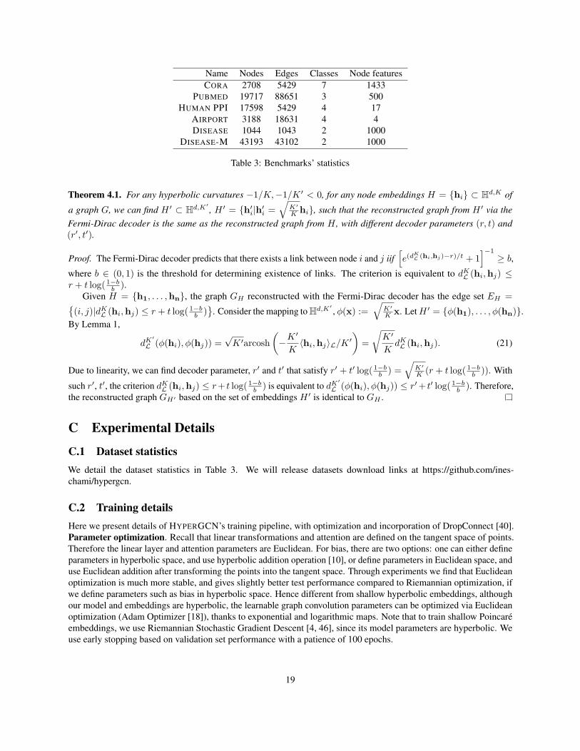
Name Nodes Edges Classes Node featuresCORA 2708 5429 7 1433

PUBMED 19717 88651 3 500HUMAN PPI 17598 5429 4 17

AIRPORT 3188 18631 4 4DISEASE 1044 1043 2 1000

DISEASE-M 43193 43102 2 1000

Table 3: Benchmarks’ statistics

Theorem 4.1. For any hyperbolic curvatures −1/K,−1/K ′ < 0, for any node embeddings H = {hi} ⊂ Hd,K of

a graph G, we can find H ′ ⊂ Hd,K′ , H ′ = {h′i|h′i =√

K′

K hi}, such that the reconstructed graph from H ′ via theFermi-Dirac decoder is the same as the reconstructed graph from H , with different decoder parameters (r, t) and(r′, t′).

Proof. The Fermi-Dirac decoder predicts that there exists a link between node i and j iif[e(dKL (hi,hj)−r)/t + 1

]−1≥ b,

where b ∈ (0, 1) is the threshold for determining existence of links. The criterion is equivalent to dKL (hi,hj) ≤r + t log( 1−b

b ).Given H = {h1, . . . ,hn}, the graph GH reconstructed with the Fermi-Dirac decoder has the edge set EH ={

(i, j)|dKL (hi,hj) ≤ r + t log( 1−bb )}

. Consider the mapping to Hd,K′ , φ(x) :=√

K′

K x. LetH ′ = {φ(h1), . . . , φ(hn)}.By Lemma 1,

dK′

L (φ(hi), φ(hj)) =√K ′arcosh

(−K

′

K〈hi,hj〉L/K ′

)=√K ′

KdKL (hi,hj). (21)

Due to linearity, we can find decoder parameter, r′ and t′ that satisfy r′ + t′ log( 1−bb ) =

√K′

K (r + t log( 1−bb )). With

such r′, t′, the criterion dKL (hi,hj) ≤ r+ t log( 1−bb ) is equivalent to dK

′

L (φ(hi), φ(hj)) ≤ r′+ t′ log( 1−bb ). Therefore,

the reconstructed graph GH′ based on the set of embeddings H ′ is identical to GH .

C Experimental Details

C.1 Dataset statisticsWe detail the dataset statistics in Table 3. We will release datasets download links at https://github.com/ines-chami/hypergcn.

C.2 Training detailsHere we present details of HYPERGCN’s training pipeline, with optimization and incorporation of DropConnect [40].Parameter optimization. Recall that linear transformations and attention are defined on the tangent space of points.Therefore the linear layer and attention parameters are Euclidean. For bias, there are two options: one can either defineparameters in hyperbolic space, and use hyperbolic addition operation [10], or define parameters in Euclidean space, anduse Euclidean addition after transforming the points into the tangent space. Through experiments we find that Euclideanoptimization is much more stable, and gives slightly better test performance compared to Riemannian optimization, ifwe define parameters such as bias in hyperbolic space. Hence different from shallow hyperbolic embeddings, althoughour model and embeddings are hyperbolic, the learnable graph convolution parameters can be optimized via Euclideanoptimization (Adam Optimizer [18]), thanks to exponential and logarithmic maps. Note that to train shallow Poincaréembeddings, we use Riemannian Stochastic Gradient Descent [4, 46], since its model parameters are hyperbolic. Weuse early stopping based on validation set performance with a patience of 100 epochs.

19

Drop connection. Since rescaling vectors in hyperbolic space requires exponential and logarithmic maps, and is con-ceptually not tied to the inverse dropout rate in terms of re-normalizing L1 norm, Dropout cannot be directly applied inHYPERGCN. However, as a result of using Euclidean parameters in HYPERGCN, DropConnect [40], the generalizationof Dropout, can be used as a regularization. DropConnect randomly zeros out the neural network connections, i.e.elements of the Euclidean parameters during training time, improving the generalization of HYPERGCN.Projections. Finally, we apply projections similar to Equations 16 and 17 for the hyperboloid model Hd,K after eachfeature transform and log or exp map, to constrain embeddings and tangent vectors to remain on the manifold andtangent spaces.

20