(Hyper)-Graphs Inference via Convex Relaxations and … · Move Making Algorithms: Contributions...
66
HAL Id: hal-01223027 https://hal.inria.fr/hal-01223027 Submitted on 1 Nov 2015 HAL is a multi-disciplinary open access archive for the deposit and dissemination of sci- entific research documents, whether they are pub- lished or not. The documents may come from teaching and research institutions in France or abroad, or from public or private research centers. L’archive ouverte pluridisciplinaire HAL, est destinée au dépôt et à la diffusion de documents scientifiques de niveau recherche, publiés ou non, émanant des établissements d’enseignement et de recherche français ou étrangers, des laboratoires publics ou privés. (Hyper)-Graphs Inference via Convex Relaxations and Move Making Algorithms: Contributions and Applications in artificial vision Pawan Kumar, Nikos Komodakis, Nikos Paragios To cite this version: Pawan Kumar, Nikos Komodakis, Nikos Paragios. (Hyper)-Graphs Inference via Convex Relaxations and Move Making Algorithms: Contributions and Applications in artificial vision. [Research Report] RR-8798, Inria. 2015, pp.65. <hal-01223027>
Transcript of (Hyper)-Graphs Inference via Convex Relaxations and … · Move Making Algorithms: Contributions...
HAL Id: hal-01223027https://hal.inria.fr/hal-01223027
Submitted on 1 Nov 2015
HAL is a multi-disciplinary open accessarchive for the deposit and dissemination of sci-entific research documents, whether they are pub-lished or not. The documents may come fromteaching and research institutions in France orabroad, or from public or private research centers.
L’archive ouverte pluridisciplinaire HAL, estdestinée au dépôt et à la diffusion de documentsscientifiques de niveau recherche, publiés ou non,émanant des établissements d’enseignement et derecherche français ou étrangers, des laboratoirespublics ou privés.
(Hyper)-Graphs Inference via Convex Relaxations andMove Making Algorithms: Contributions and
Applications in artificial visionPawan Kumar, Nikos Komodakis, Nikos Paragios
To cite this version:Pawan Kumar, Nikos Komodakis, Nikos Paragios. (Hyper)-Graphs Inference via Convex Relaxationsand Move Making Algorithms: Contributions and Applications in artificial vision. [Research Report]RR-8798, Inria. 2015, pp.65. <hal-01223027>

ISS
N02
49-6
399
ISR
NIN
RIA
/RR
--87
98--
FR
+E
NG
RESEARCHREPORT
N° 8798October 2015
Project-Teams GALEN
(Hyper)-GraphsInference via ConvexRelaxations and MoveMaking Algorithms:Contributions andApplications in artificialvisionPawan Kumar, Nikos Komodakis, Nikos Paragios


RESEARCH CENTRESACLAY – ÎLE-DE-FRANCE
Parc Orsay Université
4 rue Jacques Monod
91893 Orsay Cedex
(Hyper)-Graphs Inference via ConvexRelaxations and Move Making Algorithms:Contributions and Applications in artificial
vision
Pawan Kumar∗†, Nikos Komodakis∗‡, Nikos Paragios§
Project-Teams GALEN
Research Report n° 8798 — October 2015 — 62 pages
Abstract: Computational visual perception seeks to reproduce human vision through thecombination of visual sensors, artificial intelligence and computing. To this end, computer visiontasks are often reformulated as mathematical inference problems where the objective is to determinethe set of parameters corresponding to the lowest potential of a task-specific objective function.Graphical models have been the most popular formulation in the field over the past two decadeswhere the problem is viewed as an discrete assignment labeling one. Modularity, scalability andportability are the main strength of these methods which once combined with efficient inferencealgorithms they could lead to state of the art results. In this tutorial we focus on the inferencecomponent of the problem and in particular we discuss in a systematic manner the most commonlyused optimization principles in the context of graphical models. Our study concerns inference overlow rank models (interactions between variables are constrained to pairs) as well as as higher orderones (arbitrary set of variables determine hyper-cliques on which constraints are introduced) andseeks a concise, self-contained presentation of prior art as well as the presentation of the currentstate of the art methods in the field.
Key-words: MRFs, optimization, computer vision, convex programming, linear programming
∗ Equally contributing authors† Oxford University, UK.‡ Universite Paris-Est, École des Ponts ParisTech, France.§ CentraleSupelec, Inria, University of Paris Saclay, France.

Inférence dans les (hyper)-graphes à laide de relaxationsconvexes et dalgorithmes de coups optimisés : contributions
et applications en vision par ordinateur
Résumé : La perception numérique visuelle cherche à reproduire la vision humaine grâceà une combinaison de senseurs visuels, dintelligence artificielle et de calcul numérique. Dansce but, les problèmes de vision numériques sont souvent posés comme des problèmes dinférencemathématiques, dans lesquels lobjectif est de déterminer lensemble de paramètres correspondantau minimum dune énergie adaptée à la tâche visuelle. Les modèles graphiques ont constituéloutil de modélisation le plus populaire du domaine de ces deux dernières décennies ; le problèmey est vu comme un problème dassignation de labels discrets. La modularité, lextensibilité etla portabilité sont les atouts majeurs de ces modèles, qui combinées à des méthodes dinférenceefficaces peuvent mener à létat de lart en matière de résultats. Dans ce tutoriel nous nousfocaliseront sur le problème dinférence ; en particulier, nous discuterons de façon systématiqueles schémas doptimisation les plus utilisés dans le contexte des modèles graphiques. Notre étudeconcerne linférence sur des modèles de rang faible (où les interactions entre les variables sontlimités aux paires), ainsi que les modèles de rang supérieur (où des sous-ensemble arbitrairesde variables déterminent des hyper-cliques sur lesquels des contraintes peuvent être introduites)et vise à présenter un aperçu concis et autonome des méthodes éprouvées et à létat de lart dudomaine.
Mots-clés : MRFs, optimization, computer vision, convex programming, linear programming
(Hyper)-Graphs Inference via Convex Relaxations and Move Making Algorithms 3
1 Introduction
Graphical models (Conditional Random Fields (CRFs) or Markov Random Fields (MRFs)) havebeen introduced in the field of computer vision almost four decades ago. CRFs were introducedin [15] while MRFs were introduced in [18] to address the problem of image restoration. Thecentral idea is to express perception through an inference problem over graph. The process isdefined using a set of nodes, a set of labels, and a neighborhood system. The graph nodesoften correspond to the parameters to be determined, the labels to a quantized/discrete versionof the search space and the connectivity of the graph to the constraints/interactions betweenvariables. Graph-based methods are endowed with numerous advantages as it concerns inferencewhen compared to their alternative that refers to continuous formulations. These methods arein general gradient-free and therefore can easily accommodate changes of the model (graphstructure), changes of the objective function (perception task), or changes of the discretizationspace (precision).
Early approaches to address graph-based optimization in the field of computer vision wereprimarily based either on annealing like approaches or on local minimum update principles.Simulated annealing was an alternative direction that provides in theory good guarantees asit concerns the optimality properties of the obtained solution. The central idea is to performa search with a decreasing radius/temperature where at a given iteration the current state isupdated to a new state with a tolerance (as it concerns the objective function) that is relatedto the temperature. Such meta-heuristic methods could lead to a good approximation of theoptimal solution if temperature/radius are appropriately defined that in general is not thattrivial. Iterated conditional modes or highest confidence first were among the first attemptsexploiting local minimum iterative principles. Their underlying principle was to solve the problemprogressively through a repetitive local update of the optimal solution towards a new localoptimum. These methods were computationally efficient and deterministic in the expense ofquite inefficient in terms of capturing the global optimum of the solution and the completeabsences of guarantee as it concerns the optimality properties of the obtained solution.
Despite the elegance, modularity and scalability of MRFs/CRFs, their adoption was quitelimited (over eighties and nineties) from the image processing/computer vision community andbeyond due lack of efficient optimization methods to address their inference. The introductionof efficient inference algorithms inspired from the networks community, like for example the maxflow/min cut principle at late nineties that is a special case of the duality theorem for linearprograms as well their efficient implementations towards taking advantage of image like graphs[6] or message passing methods [50] that are based on the calculation of the marginal for a givennode given the states of the other nodes have re-introduced graphical models in the field ofcomputer vision. During the past two decades we have witnessed a tremendous progress both ontheir use to address visual perception tasks [63] as well as it concerns their inference. This tutorialaims to provide an overview of the state of the art methods in the field for inference as well asthe most recent advances in that direction using move making algorithms and convex relations.The reminder of this paper is organized as follows; Section 2 presents briefly the context and ashort review of the the most representative inference methods. Section 3 is dedicated to movemaking algorithms, while section 4 presents efficient linear programming-inspired principles forgraph inference. The last section introduces dual decomposition, a generic, modular and scalableframework to perform (hyper) graph inference.
RR n° 8798

4 Kumar, Komodakis & Paragios
2 Mathematical background: basic tools for MRF inference
2.1 Markov random fields
A Markov random field (MRF) consists of a set of random variables X = {Xp, p ∈ V}, whereV contains the set of indices of the n random variables. Each random variable can take onevalue (or label) from a set of labels L. In this manuscript, we are primarily interested in discreteMRFs, where the label set consists of a finite and discrete set of labels, that is, L = {l1, · · · , lh}.In addition, an MRF also defines a neighborhood relationship E over the random variables, thatis, (p, q) ∈ E if and only if Xp and Xq are neighboring random variables. Visually, an MRF canbe presented by a graph (V, E) whose vertices correspond to random variables and whose edgesconnected neighboring random variables.
It would be convenient to introduce the notation N (p) to denote the set of all neighbors ofthe random variable Xp. In other words, q ∈ N (p) if and only if (p, q) ∈ E. The neighborhoodrelationship defines a family of cliques C that consist of sets C ⊆ V such that any two randomvariables that belong to the same clique are neighbors of each other.
We refer to an assignment of values x ∈ Ln of all the random variables as a labeling. In orderto quantitatively distinguish among the hn possible labelings, we define an energy function whichconsists of a sum of clique potentials. Formally, the energy E(x; θ) of a labeling x is defined asfollows:
E(x; θ) =∑
C∈C
θC(xC). (1)
Here θC(xC) is the clique potential that only depends on the labels xC of the subset of variablesindexed by C ∈ V. The term θ is referred to as the parameters of the MRF.
The probability of a labeling is said to be proportional to the negative exponential of itsenergy. In other words, the lower the energy, the more probable the labeling. Thus, in order toestimate the most probable labeling, we need to solve the following energy minimization problem:
x∗ = argminx∈Ln
E(x; θ). (2)
The above problem is also referred to as maximum a posteriori inference. As a shorthand, wewill simply refer to it as inference. We note here that there also exist other types of inferenceproblems, such as computing the marginal probability of a subset of random variables. However,these problems are out of scope for the current manuscript.
An important special case of MRFs that is widely studied in the literature is that of pairwiseMRFs, which consists of two types of clique potentials. First, unary potentials θp(xp), whichdepend on the label of one random variable p ∈ V. Second, pairwise potentials θpq(xp,xq), whichdepend on the labels of two neighboring random variables Xp and Xq. In other words, given apairwise MRF, the energy of a labeling x is specified as follows:
E(x; θ) =∑
p∈V
θp(xp) +∑
(p,q)∈E
θpq(xp,xq). (3)
Note that, even with the restriction imposed by pairwise MRFs on the form of the energy function,inference remains an NP-hard problem. However, there are some special cases that admit moreefficient exact algorithms, which we will briefly describe in the remainder of the chapter. Thesealgorithms will form the building blocks for the more complex state of the art inference algorithmsfor both pairwise and general high-order MRFs in subsequent chapters.
Inria

(Hyper)-Graphs Inference via Convex Relaxations and Move Making Algorithms 5
2.2 Reparameterization
Before we delve into the details of some well-known exact inference algorithms for special casesof pairwise MRFs, we first need to define the important concept of reparameterization. Two setsof parmeters θ and θ′ are said to be reparameterizations of each other if they specify the sameenergy value for all possible labelings, that is,
E(x; θ) = E(x; θ′), ∀x ∈ Ln. (4)
For pairwise MRFs, a sufficient condition for two parameters θ and θ′ to be reparameterizationsof each other is that there exist scalars Mpq(lj) and Mqp(li) for all (p, q) ∈ E and li, lj ∈ L suchthat
θ′pq(li, lj) = θpq(li, lj)−Mpq(lj)−Mqp(li),
θ′p(li) = θp(li) +∑
q∈N (p)
Mqp(li). (5)
Interestingly, the above equation is also a necessary condition for reparameterization [29]. How-ever, for the purposes of this manuscript, it is sufficient to understand why the above conditionis sufficient for reparameterization. Intuitively, the unary potential θ′p(li) introduces an extrapenalty Mqp(li) for assinging the label li to p. However, since the random variable q also needsto be assigned exactly one label, say lj , this extra penalty is canceled out in the correspondingpairwise potential θ′pq(li, lj). This ensures that θ and θ′ are reparameterizations of each other.The concept of reparametrization is fundamental to the design of inference algorithms. Specif-ically, most inference algorithms can be viewed as a series of reparameterizations of the givenMRF such that the resulting set of parameters make it easy to minimize the energy over allpossible labelings.
2.3 Dynamic programming
We are now ready to describe our first inference algorithm—dynamic programming—that is exactfor tree-structured MRFs. In other words, if we visualize an MRF as a graph (V, E), then it hasto be singly connected (that is, without any cycles or loops).
It would be helpful to first consider a simple chain MRF defined over n random variablesV = {1, · · · ,n} such that E = {(p, p + 1), p = 1, · · · ,n − 1}. In other words, two randomvariables p and p + 1 are neighbors of each other, thus forming a graph that resembles a chain.A visual representation of an example chain MRF over four random variables along with thecorresponding potential values is provided in Figure 1. Inference on a chain MRF can be specifiedas the following optimization problem:
minx∈Ln
∑
p∈V
θp(xp) +∑
(p,q)∈E
θpq(xp,xq)
= minx∈Ln
(θ1(x1) + θ12(x1,x2)+
∑
p∈V\{1}
θp(xp) +∑
(p,q)∈E\{(1,2)}
θpq(xp,xq)
. (6)
Here, the operator ‘\’ represents the set difference. The above reformulation of inference explicitlyconsiders all the terms that are dependent on the label x1. In order to solve the above problem,we will obtain a clever reparameterization that reduces it to an equivalent problem defined on a
RR n° 8798

6 Kumar, Komodakis & Paragios
Figure 1: An example chain MRF over four random variables X = {X1,X2,X3,X4}, that is,V = {1, 2, 3, 4}. Each random variable is depicted as an unfilled circle and can take one label fromthe set L = {l1, l2}. The labels are shown as branches on the trellises on top of the correspondingrandom variable. The unary potential value θp(li) is shown next to the i-th branch of the randomvariable Xp. For example, θ1(l1) = 5 and θ2(l2) = 4. Similarly, the pairwise potential valueθpq(li, lj) is shown next to the connection between the i-th branch of Xp and the j-th branch ofXq respectively. For example, θ12(l1, l2) = 1 and θ34(l2, l1) = 4.
chain MRF with n−1 random variables. To this end, we choose the following reparameterizationconstants:
M12(lj) = minli∈L
θ1(li) + θ12(li, lj). (7)
Using the above constants, we obtain a reparameterization θ′ of the original parameters θ asfollows:
θ′2(lj) = θ2(lj) +M12(lj), ∀lj ∈ L, (8)
θ′12(li, lj) = θ12(li, lj)−M12(lj), ∀li, lj ∈ L,
θ′p(li) = θp(li), ∀p ∈ V\{2}, li ∈ L,
θ′pq(li, lj) = θpq(li, lj), ∀(p, q) ∈ E\{(1, 2)}, li, lj ∈ L.
In other words, we modify the unary potential of the second random variable by adding thecorresponding reparameterization constants and the pairwise potential between the first andthe second random variable by subtracting the corresponding reparametrization constants. Theremaining potentials remain unchanged. The total time complexity of obtaining the above repa-rameterization is O(h2) since we need to compute O(h) constants, each of which takes O(h) timeto compute using equation (7). The advantage of the above reparameterization is that for allvalues of lj ∈ L the following holds true:
minliθ′1(li) + θ′12(li, lj) = 0. (9)
In other words, for any choice of label lj , we can choose a label li such that the contributionof the potentials that depend on li is 0. Note that this since we are interested in minimizingthe energy over all possible labeling, this choice of li will be an optimal one as other choicescannot contribute a negative term to the energy. Using this fact, we can rewrite the inference
Inria

(Hyper)-Graphs Inference via Convex Relaxations and Move Making Algorithms 7
problem (6) as follows:
minx∈Ln
(θ′1(x1) + θ′12(x1,x2)+
∑
p∈V\{1}
θ′p(xp) +∑
(p,q)∈E\{(1,2)}
θ′pq(xp,xq)
= minx∈Ln−1
∑
p∈V\{1}
θ′p(xp) +∑
(p,q)∈E\{(1,2)}
θ′pq(xp,xq).
The first problem is equivalent to problem (6) since θ′ is a reparameterization of θ. The secondproblem is equivalent to the first problem since the optimum choice of x1 for any value of x2
provides a contribution of 0 to the energy function.The above argument shows that it is possible to reduce an inference problem on a chain MRF
with n random variables to a chain MRF with n−1 random variables in O(h2) time. Taking thisargument forward, we can start from one end of the chain and move to the other end in n − 1steps. At step p, we can reparameterize the MRF by using constants:
Mpq(lj) = minli∈L
θp(li) + θpq(li, lj), (10)
where q = p + 1 and θ is the current set of parameters. At the end of step n − 1, we obtain areparameterization θ that corresponds to a problem of a chain MRF of size 1. In other words,the energy of the optimum labeling can be computed as minl∈L θn(l). The total time complexityof the algorithm is O(nh2), since each step has a complexity of O(h2) and there are O(n) stepsin total.
Note that we can not only compute the minimum energy over all possible labelings, but alsoan optimal labeling itself. To achieve this, we simply need to keep track of the label xp thatis the optimal for every label xp+1 of the random variable p + 1, that is, the label li that isused to compute the reparameterization constant in equation (10). At the end of step n− 1, wecan compute the optimal label of the variable n as x∗n = argminl∈L θn(l), and then backtrackto obtain the optimal label of all the random variables. Figure 2 shows the steps of dynamicprogramming for the chain MRF depicted in Figure 1.
In summary, dynamic programming for a chain MRF starts from one end of the chain andmoves to the other end. At each step, it reparameterizes the current edge (p, q), where theconstants are computed using equation (10). This algorithm can be extended to the more generaltree-structured MRFs using the same technique of reparameterization. The key observation isthat the sequence of reparameterization would proceed from the leaf random variables to theroot random variable, where once again the reparameterization constants are computed usingequation (10). Once we reach the root random variable Xn, we can compute the minimum energyas minl∈L θn(l), where θ is the final reparameterization obtained by dynamic programming.Similar to the chain MRF case, we can also obtain the optimal labeling by keeping track of theoptimal label to assign to a child random variable for each possible label of its parent randomvariable. Note that since we have made no assumptions regarding the form of the pairwisepotentials, the reparameterization constant for each edge take O(h2) time to compute. However,for many special cases of pairwise potentials, the computation of reparameterization constantscan be significantly speeded up. We refer the interested reader to [14] for details.
2.4 Message passing and belief propagation
The above description of dynamic programming suggests an implementation based on reparame-terizing the edges of a given tree-structured MRF. An alternative way to view the above algorithm
RR n° 8798

8 Kumar, Komodakis & Paragios
Figure 2: The three steps of reparameterization required by the dynamic programming algorithmto perform inference on the chain MRF depicted in Figure 1. In the first step (top row), repa-rameterization affects the unary potentials of X2 and the pairwise potentials of (X1,X2). Thereparameterization constants are computed using equation (10). The figure also shows the optimallabel of X1 for the label l1 (at the top) and the label l2 (at the bottom) of X2. This informationis used to compute the optimal labeling of the chain MRF. Similarly, the reparameterization cor-responding to (X2,X3) and (X3,X4) is shown in the middle and bottom row respectively. Afterthree iterations, we can determine the optimal label for X4 as l2, which implies that the optimallabel for X3, X2 and X1 is l1, l1 and l2 respectively. The energy of the optimal labeling is 13.
Inria

(Hyper)-Graphs Inference via Convex Relaxations and Move Making Algorithms 9
is via iterative message passing [50]. At each iteration, a random variable p passes a message toeach of its neighbors q ∈ N (p) (one message per neighbor). The message that p passes to q isa vector mpq of size h = |L|. In other words, it contains one scalar for each label lj , which isspecified as follows:
mpq(lj) = minli∈L
θp(li) + θpq(li, lj) +∑
r∈N (p)\{q}
mrp(li)
+ η1. (11)
Here, η1 is a constant that is used to prevent numerical overflow or underflow. The messages areused to compute the beliefs of a random variable p in a label li as follows:
belp(li) = θp(li) +∑
q∈N (p)
mqp(li) + η2. (12)
Again, η2 is a constant that prevents numerical instability. Given a tree-structured MRF, wecan choose to pass the messages starting from the leaf random variables and moving up to theroot random variable. In this case, it can be shown that the above message passing algorithmis equivalent to the reparameterization based dynamic programming algorithm described in theprevious section [29]. Interestingly, [50] proved that the following generalization of the algorithmcan also be used to obtain the optimal labeling of a tree-structured MRF: (i) pass messages inany arbitrary order; and (ii) terminate the algorithm when the messages do not changes fromone iteration to the next. At convergence, the optimal label of each random variable p can beobtained as x∗p = argminl∈L belp(l).
The above message passing algorithm, commonly referred to as belief propagation, is guaran-teed to be optimal for a tree-structured MRF. However, for a general MRF, belief propagationis not even guaranteed to converge in a finite number of iterations. Nonetheless, it is commonlyused as an approximate inference algorithm in practice [45].
2.5 Graph cuts
The previous two sections describe an efficient exact inference algorithm for tree-structuredMRFs. Another special case that admits an efficient exact algorithm is when the energy func-tion is submodular. Formally, a pairwise energy function E(x; θ) is submodular if the pairwisepotentials for all (p, q) ∈ E satisfy the following inequality:
θpq(li, li+1) + θpq(lj , lj+1) ≤ θpq(li, lj+1) + θpq(lj , li+1), ∀i, j ∈ {1, · · · ,h− 1}. (13)
Note that the submodularity condition places no restrictions on the form of the unary potentials.Specifically, the minimization of a submodular energy function over all possible labelings can bemapped to an equivalent st-MINCUT problem for which several efficient algorithms have beenproposed in the literature [4]. We briefly describe how a binary submodular energy function(that is, an energy function defined using a label set of size 2) can be mapped to an st-MINCUTproblem. For the more general setting of h ≥ 2 labels, we refer the reader to [23, 17] for details.Before describing the mapping, we briefly define the st-MINCUT problem for completeness.
The st-MINCUT problem. We are given a directed graph D = (N, A) where N is the setof nodes (vertices) and A is the set of arcs. Associated with each arc (Np,Nq) ∈ A is a non-negative capacity c(Np,Nq). Given two nodes s, t ∈ N, known as terminals, an st-cut is definedas the outgoing arcs from a subset of nodes N1 to another subset of nodes N2 such that thefollowing conditions holds: (i) s ∈ N1; (ii) t ∈ N2; (iii) N1∩N2 = {}; and (iv) N1∪N2 = N. In
RR n° 8798
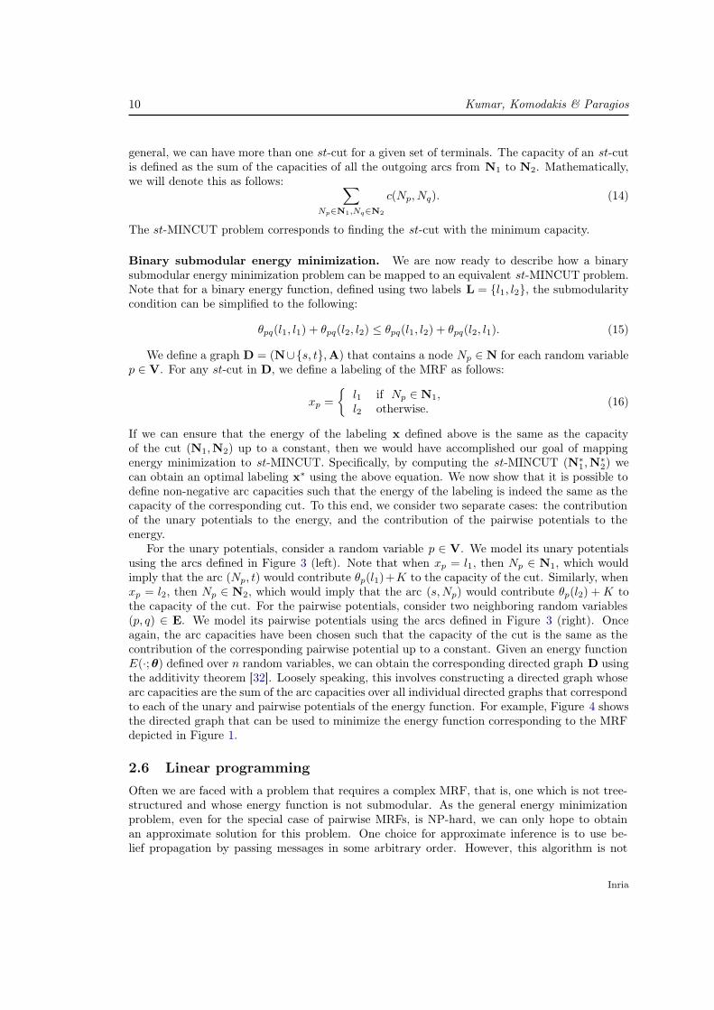
10 Kumar, Komodakis & Paragios
general, we can have more than one st-cut for a given set of terminals. The capacity of an st-cutis defined as the sum of the capacities of all the outgoing arcs from N1 to N2. Mathematically,we will denote this as follows: ∑
Np∈N1,Nq∈N2
c(Np,Nq). (14)
The st-MINCUT problem corresponds to finding the st-cut with the minimum capacity.
Binary submodular energy minimization. We are now ready to describe how a binarysubmodular energy minimization problem can be mapped to an equivalent st-MINCUT problem.Note that for a binary energy function, defined using two labels L = {l1, l2}, the submodularitycondition can be simplified to the following:
θpq(l1, l1) + θpq(l2, l2) ≤ θpq(l1, l2) + θpq(l2, l1). (15)
We define a graph D = (N∪{s, t}, A) that contains a node Np ∈ N for each random variablep ∈ V. For any st-cut in D, we define a labeling of the MRF as follows:
xp =
{l1 if Np ∈ N1,l2 otherwise.
(16)
If we can ensure that the energy of the labeling x defined above is the same as the capacityof the cut (N1, N2) up to a constant, then we would have accomplished our goal of mappingenergy minimization to st-MINCUT. Specifically, by computing the st-MINCUT (N∗1, N∗2) wecan obtain an optimal labeling x∗ using the above equation. We now show that it is possible todefine non-negative arc capacities such that the energy of the labeling is indeed the same as thecapacity of the corresponding cut. To this end, we consider two separate cases: the contributionof the unary potentials to the energy, and the contribution of the pairwise potentials to theenergy.
For the unary potentials, consider a random variable p ∈ V. We model its unary potentialsusing the arcs defined in Figure 3 (left). Note that when xp = l1, then Np ∈ N1, which wouldimply that the arc (Np, t) would contribute θp(l1)+K to the capacity of the cut. Similarly, whenxp = l2, then Np ∈ N2, which would imply that the arc (s,Np) would contribute θp(l2) + K tothe capacity of the cut. For the pairwise potentials, consider two neighboring random variables(p, q) ∈ E. We model its pairwise potentials using the arcs defined in Figure 3 (right). Onceagain, the arc capacities have been chosen such that the capacity of the cut is the same as thecontribution of the corresponding pairwise potential up to a constant. Given an energy functionE(·; θ) defined over n random variables, we can obtain the corresponding directed graph D usingthe additivity theorem [32]. Loosely speaking, this involves constructing a directed graph whosearc capacities are the sum of the arc capacities over all individual directed graphs that correspondto each of the unary and pairwise potentials of the energy function. For example, Figure 4 showsthe directed graph that can be used to minimize the energy function corresponding to the MRFdepicted in Figure 1.
2.6 Linear programming
Often we are faced with a problem that requires a complex MRF, that is, one which is not tree-structured and whose energy function is not submodular. As the general energy minimizationproblem, even for the special case of pairwise MRFs, is NP-hard, we can only hope to obtainan approximate solution for this problem. One choice for approximate inference is to use be-lief propagation by passing messages in some arbitrary order. However, this algorithm is not
Inria

(Hyper)-Graphs Inference via Convex Relaxations and Move Making Algorithms 11
Figure 3: Left. The directed graph corresponding to unary potentials. The constant K is chosento be sufficiently large to ensure that the arc capacities are non-negative. Note that since therandom variable p has to be assigned exactly one label, adding a constant to the arc capacities of(s,Np) and (Np, t) simply adds a constant to the capacity of every st-cut, thereby not affectingthe st-MINCUT solution. Right. The directed graph corresponding to the pairwise potentials.The constants K1 and K2 ensure that the arc capacities are non-negative. The arc capacityP = θpq(l1, l2) + θpq(l2, l1) − θpq(l1, l1) − θpq(l2, l2) is guaranteed to be non-negative due to thesubmodularity of the energy function (see equation (15)).
Figure 4: The directed graph D corresponding to the submodular energy function of the MRFdepicted in Figure 1. Any st-cut of D has a corresponding labeling for the MRF, defined byequation (16), such that the capacity of the cut is equal to the energy of the labeling plus aconstant. Hence, the minimum st-cut of D provides an optimal labeling of the MRF.
RR n° 8798
12 Kumar, Komodakis & Paragios
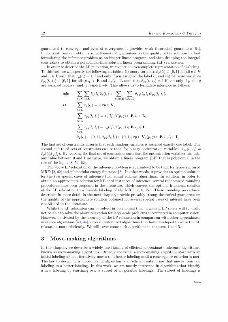
guaranteed to converge, and even at covergence, it provides weak theoretical guarantees [64].In contrast, one can obtain strong theoretical guarantees on the quality of the solution by firstformulating the inference problem as an integer linear program, and then dropping the integralconstraints to obtain a polynomial-time solution linear programming (LP) relaxation.
In order to describe the LP relaxation, we require an overcomplete representation of a labeling.To this end, we will specify the following variables: (i) unary variables xp(li) ∈ {0, 1} for all p ∈ Vand li ∈ L such that xp(li) = 1 if and only if p is assigned the label li; and (ii) pairwise variablesxpq(li, lj) ∈ {0, 1} for all (p, q) ∈ E and li, lj ∈ L such that xpq(li, lj) = 1 if and only if p and qare assigned labels li and lj respectively. This allows us to formulate inference as follows:
minx
∑
p∈V
∑
li∈L
θp(li)xp(li) +∑
(p,q)∈E
∑
li,lj∈L
θpq(li, lj)xpq(li, lj),
s.t.∑
li∈L
xp(li) = 1, ∀p ∈ V,
∑
lj∈L
xpq(li, lj) = xp(li), ∀(p, q) ∈ E, li ∈ L,
∑
li∈L
xpq(li, lj) = xq(lj), ∀(p, q) ∈ E, lj ∈ L,
xp(li) ∈ {0, 1}, xpq(li, lj) ∈ {0, 1}, ∀p ∈ V, (p, q) ∈ E, li, lj ∈ L.
The first set of constraints ensures that each random variables is assigned exactly one label. Thesecond and third sets of constraints ensure that, for binary optimization variables, xpq(li, lj) =xp(li)xq(lj). By relaxing the final set of constraints such that the optimization variables can takeany value between 0 and 1 inclusive, we obtain a linear program (LP) that is polynomial in thesize of the input [8, 54, 62].
The above LP relaxation of the inference problem is guaranteed to be tight for tree-structuredMRFs [2, 62] and submodular energy functions [8]. In other words, it provides an optimal solutionfor the two special cases of inference that admit efficient algorithms. In addition, in order toobtain an approximate solution for NP-hard instances of inference, several randomized roundingprocedures have been proposed in the literature, which convert the optimal fractional solutionof the LP relaxation to a feasible labeling of the MRF [2, 8, 27]. These rounding procedures,described in more detail in the next chapter, provide provably strong theoretical guarantees onthe quality of the approximate solution obtained for several special cases of interest have beenestablished in the literature.
While the LP relaxation can be solved in polynomial time, a general LP solver will typicallynot be able to solve the above relaxation for large-scale problems encountered in computer vision.However, motivated by the accuracy of the LP relaxation in comparison with other approximateinference algorithms [40, 44], several customized algorithms that have developed to solve the LPrelaxation more efficiently. We will cover some such algorithms in chapters 4 and 5.
3 Move-making algorithms
In this chapter, we describe a widely used family of efficient approximate inference algorithms,known as move-making algorithms. Broadly speaking, a move-making algorithm start with aninitial labeling x0 and iteratively moves to a better labeling until a convergence criterion is met.The key to designing a move-making algorithm is an efficient subroutine that moves from onelabeling to a better labeling. In this work, we are mostly interested in algorithms that identifya new labeling by searching over a subset of all possible labelings. The subset of labelings is
Inria

(Hyper)-Graphs Inference via Convex Relaxations and Move Making Algorithms 13
chosen to satisfy the following two conditions: (i) it contains the current labeling; and (ii) itallows us to identify a new (possibly better) labeling by solving a single st-MINCUT problem.Since st-MINCUT admits several efficient algorithm, each iteration of a move-making algorithmwill also be efficient. Typically, the move-making algorithms also converge in a small numberof iterations, thereby making the whole procedure computationally feasible for even large-scaleproblems encountered in computer vision.
We begin our exploration of move-making algorithms by considering a special case of inferenceknown as metric labeling, which is commonly used to model low-level vision applications. Lateron in the chapter we will consider high-order energy functions that are amenable to move-making algorithms. Metric labeling is characterized by a finite, discrete label set and a metricdistance function over the labels. The energy function in metric labeling consists of arbitraryunary potentials and pairwise potentials that are proportional to the distance between the labelsassigned to them. The problem is known to be NP-hard [60]. Traditionally, in the computer visioncommunity, this problem is solved approximately one of several move-making algorithms [5, 20,39, 41, 61]. The advantage of move-making algorithms is their computational efficiency. However,most of the early move-making algorithms provide weaker theoretical guarantees on the qualityof the solution than the slower LP relaxation discussed in the previous chapter.
At first sight, the difference between move-making algorithms and the LP relaxation appearsto be the standard accuracy vs. speed trade-off. However, for some special cases of distancefunctions, it has been shown that appropriately designed move-making algorithms can match thetheoretical guarantees of the LP relaxation [39, 41, 60]. Recently, this result has been extendedfor a large class of randomized rounding procedures, which we call parallel rounding [38]. Inparticular it has been shown that for any arbitrary (semi-)metric distance function, there existmove-making algorithms that match the theoretical guarantees provided by parallel rounding.In the following sections, we study such rounding-based move-making algorithms in detail.
3.1 Preliminaries
Metric labeling. A metric labeling problem is a special case of inference that is defined usinga metric distance function d : L×L→ R+ over the labels. Recall that a metric distance functionsatisfies the following properties: (i) d(li, lj) ≥ 0 for all li, lj ∈ L, and d(li, lj) = 0 if and only ifi = j; and (ii) d(li, lj) + d(lj , lk) ≥ d(li, lk) for all li, lj , lk ∈ L. The energy function consists ofarbitrary unary potentials, and pairwise potentials that are proportional to the distance betweenthe two labels. Formally, the energy of a labeling x is
E(x) =∑
p∈V
θp(xp) +∑
(p,q)∈E
wpqd(xp,xq), (17)
where the edge weights wpq are non-negative. Metric labeling requires us to find a labeling withthe minimum energy. It is known to be NP-hard, and hence, we have to settle for an approximatesolution.
Multiplicative bound. As metric labeling plays a central role in low-level vision, severalapproximate algorithms have been proposed in the literature. A common theoretical measure ofaccuracy for an approximate algorithm is the multiplicative bound. In this work, we are interestedin the multiplicative bound of an algorithm with respect to a distance function. Formally, givena distance function d, the multiplicative bound of an algorithm is said to be B if the followingcondition is satisfied for all possible values of unary potentials θp(·) and non-negative edge weights
RR n° 8798

14 Kumar, Komodakis & Paragios
wpq: ∑
p∈V
θp(x′p) +
∑
(p,q)∈E
wpqd(x′p,x′q) ≤
∑
p∈V
θp(x∗p) +B
∑
(p,q)∈E
wpqd(x∗p,x∗q). (18)
Here, x′ is the labeling estimated by the algorithm for the given values of unary potentials andedge weights, and x∗ is an optimal labeling. Multiplicative bounds are greater than or equalto 1, and are invariant to reparameterizations that only modify the unary potentials. Notethat reparameterizations that modify the pairwise potentials are not considered since the energyfunction needs to have a specific form for a valid metric labeling problem. A multiplicativebound B is said to be tight if the above inequality holds as an equality for some value of unarypotentials and edge weights.
Rounding procedure. In order to prove theoretical guarantees of the LP relaxation, it iscommon to use a rounding procedure that can covert a feasible fractional solution x of theLP relaxation to a feasible integer solution x of the integer linear program. Several roundingprocedures have been proposed in the literature. In this work, we focus on the randomizedparallel rounding procedures proposed by chekuri and kleinbergstoc99. These procedures havethe property that, given a fractional solution x, the probability of assigning a label li ∈ L to arandom variable p ∈ V is equal to xp(li), that is,
Pr(xp(li) = 1) = xp(li). (19)
We will describe the various rounding procedures in detail in sections 3.2-3.4. For now, we wouldlike to note that our reason for focusing on the parallel rounding of chekuri and kleinbergstoc99is that they provide the best known polynomial-time theoretical guarantees for metric labeling.Specifically, we are interested in their approximation factor, which is defined next.
Approximation factor. Given a distance function d, the approximation factor for a roundingprocedure is said to be F if the following condition is satisfied for all feasible fractional solutionsx:
E
∑
li,lj∈L
d(li, lj)xp(li)xq(lj)
≤ F∑
li,lj∈L
d(li, lj)xab(li, lj). (20)
Here, x refers to the integer solution, and the expectation is taken with respect to the randomizedrounding procedure applied to the feasible solution x.
Given a rounding procedure with an approximation factor of F , an optimal fractional solutionx∗ of the LP relaxation can be rounded to a labeling x that satisfies the following condition:
E
∑
p∈V
∑
li∈L
θp(li)xp(li) +∑
(p,q)∈E
∑
li,lj∈L
wpqd(li, lj)xp(li)xq(lj)
≤∑
p∈V
∑
li∈L
θa(li)x∗p(li) + F
∑
(p,q)∈E
∑
li,lj∈L
wpqd(li, lj)x∗pq(li, lj).
The above inequality follows directly from properties (19) and (20). Similar to multiplicativebounds, approximation factors are always greater than or equal to 1, and are invariant to repa-rameterizations that only modify the unary potentials. An approximation factor F is said to betight if the above inequality holds as an equality for some value of unary potentials and edgeweights.
Inria

(Hyper)-Graphs Inference via Convex Relaxations and Move Making Algorithms 15
Submodular energy function. We will use the following important fact throughout thischapter. Given an energy function defined using arbitrary unary potentials, non-negative edgeweights and a submodular distance function, an optimal labeling can be computed in polynomialtime by solving an equivalent minimum st-cut problem [17]. Recall that a submodular distancefunction d′ over a label set L = {l1, l2, · · · , lh} satisfies the following properties: (i) d′(li, lj) ≥ 0for all li, lj ∈ L, and d′(li, lj) = 0 if and only if i = j; and (ii) d′(li, lj) + d′(li+1, lj+1) ≤d′(li, lj+1) + d′(li+1, lj) for all li, lj ∈ L\{lh} (where \ refers to set difference).
3.2 Complete rounding and complete move
We start with a simple rounding scheme, which we call complete rounding. While completerounding is not very accurate, it would help illustrate the flavor of rounding-based moves. Wewill subsequently consider its generalizations, which have been useful in obtaining the best-knownapproximation factors for various special cases of metric labeling.
The complete rounding procedure consists of a single stage where we use the set of all unaryvariables to obtain a labeling (as opposed to other rounding procedures discussed subsequently).Algorithm 1 describes its main steps. Intuitively, it treats the value of the unary variable xp(li)as the probability of assigning the label li ∈ L to the random variable p ∈ V. It obtains alabeling by sampling from all the distributions xp = [xp(li), ∀li ∈ L] simultaneously using thesame random number r ∈ [0, 1].
It can be shown that using a different random number to sample the distributions xp and xqof two neighboring random variables (p, q) ∈ E results in an infinite approximation factor. Forexample, let xa(li) = xq(li) = 1/h for all li ∈ L, where h is the number of labels. The pairwisevariables xpq that minimize the energy function are xpq(li, li) = 1/h and xpq(li, lj) = 0 wheni 6= j. For the above feasible solution of the LP relaxation, the RHS of inequality (20) is 0 forany finite F , while the LHS of inequality (20) is strictly greater than 0 if h > 1. However, wewill shortly show that using the same random number r for all random variables provides a finiteapproximation factor.
Algorithm 1 The complete rounding procedure.input A feasible solution x of the LP relaxation.1: Pick a real number r uniformly from [0, 1].2: for all p ∈ V do3: Define xp(0) = 0 and xp(i) =
∑ij=1 xp(lj) for all li ∈ L.
4: Assign the label li ∈ L to the random variable p if xp(i− 1) < r ≤ xp(i).5: end for
We now turn our attention to designing a move-making algorithm whose multiplicative boundmatches the approximation factor of the complete rounding procedure. To this end, we modifythe range expansion algorithm proposed by kumarnips08 for truncated convex pairwise potentialsto a general (semi-)metric distance function. Our method, which we refer to as the completemove-making algorithm, considers all putative labels of all random variables, and provides anapproximate solution in a single iteration. Algorithm 2 describes its two main steps. First, itcomputes a submodular overestimation of the given distance function by solving the following
RR n° 8798

16 Kumar, Komodakis & Paragios
optimization problem:
dS = argmind′
t (21)
s.t. d′(li, lj) ≤ td(li, lj), ∀li, lj ∈ L,
d′(li, lj) ≥ d(li, lj), ∀li, lj ∈ L,
d′(li, lj) + d′(li+1, lj+1) ≤ d′(li, lj+1) + d′(li+1, lj), ∀li, lj ∈ L\{lh}.
The above problem minimizes the maximum ratio of the estimated distance to the originaldistance over all pairs of labels, that is,
maxi 6=j
d′(li, lj)d(li, lj)
.
We will refer to the optimal value of problem (21) as the submodular distortion of the distancefunction d. Second, it replaces the original distance function by the submodular overestimationand computes an approximate solution to the original metric labeling problem by solving asingle minimum st-cut problem. Note that, unlike the range expansion algorithm [41] that usesthe readily available submodular overestimation of a truncated convex distance (namely, thecorresponding convex distance function), our approach estimates the submodular overestimationvia the LP (21). Since the LP (21) can be solved for any arbitrary distance function, it makescomplete move-making more generally applicable.
Algorithm 2 The complete move-making algorithm.input Unary potentials θp(·), edge weights wpq, distance function d.1: Compute a submodular overestimation of d by solving problem (21).2: Using the approach of flachtr06, solve the following problem via an equivalent minimumst-cut problem:
x′ = argminx∈Ln
∑
p∈V
θp(xp) +∑
(p,q)∈E
wpqdS(xp,xq).
The following theorem establishes the theoretical guarantees of the complete move-makingalgorithm and the complete rounding procedure. The tight multiplicative bound of the completemove-making algorithm is equal to the submodular distortion of the distance function. Further-more, the tight approximation factor of the complete rounding procedure is also equal to thesubmodular distortion of the distance function.
In terms of computational complexities, complete move-making is significantly faster thansolving the LP relaxation. Specifically, given an MRF with n random variables (that is, |V| = n)and m edges (that is, |E| = m), and a label set with h labels (that is, |L| = h), the LP relaxationrequires at least O(m3h3 log(m2h3)) time, since it consists of O(mh2) optimization variables andO(mh) constraints. In contrast, complete move-making requires O(nmh3 log(m)) time, since thegraph constructed using the method of flachtr06 consists of O(nh) nodes and O(mh2) arcs. Notethat complete move-making also requires us to solve the linear program (21). However, sinceproblem (21) is independent of the unary potentials and the edge weights, it only needs to besolved once beforehand in order to compute the approximate solution for any metric labelingproblem defined using the distance function d.
3.3 Interval rounding and interval moves
Theorem 3.2 implies that the approximation factor of the complete rounding procedure is verylarge for distance functions that are highly non-submodular. For example, consider the truncated
Inria

(Hyper)-Graphs Inference via Convex Relaxations and Move Making Algorithms 17
linear distance function defined as follows over a label set L = {l1, l2, · · · , lh}:
d(li, lj) = min{|i− j|,M}.
Here, M is a user specified parameter that determines the maximum distance. The tightestsubmodular overestimation of the above distance function is the linear distance function, thatis, d(li, lj) = |i− j|. This implies that the submodular distortion of the truncated linear metricis (h − 1)/M , and therefore, the approximation factor for the complete rounding procedure isalso (h− 1)/M . In order to avoid this large approximation factor, chekuri proposed an intervalrounding procedure, which captures the intuition that it is beneficial to assign similar labels toas many random variables as possible.
Algorithm 3 provides a description of interval rounding. The rounding procedure chooses aninterval of at most a consecutive labels (step 2). It generates a random number r (step 3), anduses it to attempt to assign labels to previously unlabeled random variables from the selectedinterval (steps 4-7). It can be shown that the overall procedure converges in a polynomial numberof iterations with a probability of 1 [8]. Note that if we fix a = h and z = 1, interval roundingbecomes equivalent to complete rounding. However, the analyses of chekuri and kleinbergstoc99shows that other values of a provide better approximation factors for various special cases.
Algorithm 3 The interval rounding procedure.input A feasible solution x of the LP relaxation.1: repeat2: Pick an integer z uniformly from [−a+ 2,h]. Define an interval of labels I = {ls, · · · , le},
where s = max{z, 1} is the start index and e = min{z + a− 1,h} is the end index.3: Pick a real number r uniformly from [0, 1].4: for all Unlabeled random variables p do5: Define xp(0) = 0 and xp(i) =
∑s+i−1j=s xp(lj) for all i ∈ {1, · · · , e− s+ 1}.
6: Assign the label ls+i−1 ∈ I to the p if xp(i− 1) < r ≤ xp(i).7: end for8: until All random variables have been assigned a label.
Our goal is to design a move-making algorithm whose multiplicative bound matches theapproximation factor of interval rounding for any choice of a. To this end, we propose theinterval move-making algorithm that generalizes the range expansion algorithm [41], originallyproposed for truncated convex distances, to arbitrary distance functions. Algorithm 4 providesits main steps. The central idea of the method is to improve a given labeling x′ by allowing eachrandom variable p to either retain its current label x′p or to choose a new label from an intervalof consecutive labels. In more detail, let I = {ls, · · · , le} ⊆ L be an interval of labels of length atmost a (step 4). For the sake of simplicity, let us assume that x′p /∈ I for any random variable p.We define Ip = I
⋃{x′p} (step 5). For each pair of neighboring random variables (p, q) ∈ E, we
compute a submodular distance function dSx′p,x′q: Ip × Iq → R+ by solving the following linear
RR n° 8798

18 Kumar, Komodakis & Paragios
program (step 6):
dSx′p,x′q= argmin
d′t (22)
s.t. d′(li, lj) ≤ td(li, lj), ∀li ∈ Ip, lj ∈ Iq,
d′(li, lj) ≥ d(li, lj), ∀li ∈ Ip, lj ∈ Iq,
d′(li, lj) + d′(li+1, lj+1) ≤ d′(li, lj+1) + d′(li+1, lj), ∀li, lj ∈ I\{le},
d′(li, le) + d′(li+1,x′q) ≤ d′(li,x
′q) + d′(li+1, le), ∀li ∈ I\{le},
d′(le, lj) + d′(x′p, lj+1) ≤ d′(le, lj+1) + d′(x′p, lj), ∀lj ∈ I\{le},
d′(le, le) + d(x′p,x′q) ≤ d
′(le,x′q) + d′(x′p, le).
Similar to problem (21), the above problem minimizes the maximum ratio of the estimateddistance to the original distance. However, instead of introducing constraints for all pairs oflabels, it is only considers pairs of labels li and lj where li ∈ Ip and lj ∈ Iq. Furthermore, itdoes not modify the distance between the current labels x′p and x′q (as can be seen in the lastconstraint of problem (22)).
Given the submodular distance functions dSx′p,x′q, we can compute a new labeling x′′ by solving
the following optimization problem via minimum st-cut using the method of flachtr06 (step 7):
x′′ = argminx
∑
p∈V
θp(xp) +∑
(p,q)∈E
wpqdSx′p,x′q
(xp,xq)
s.t. xp ∈ Ia, ∀p ∈ V. (23)
If the energy of the new labeling x′′ is less than that of the current labeling x′, then we updateour labeling to x′′ (steps 8-10). Otherwise, we retain the current estimate of the labeling andconsider another interval. The algorithm converges when the energy does not decrease for anyinterval of length at most a. Note that, once again, the main difference between interval move-making and the range expansion algorithm is the use of an appropriate optimization problem,namely the LP (22), to obtain a submodular overestimation of the given distance function. Thisallows us to use interval move-making for the general metric labeling problem, instead of focusingon only truncated convex models.
The following theorem establishes the theoretical guarantees of the interval move-makingalgorithm and the interval rounding procedure. The tight multiplicative bound of the inter-val move-making algorithm is equal to the tight approximation factor of the interval roundingprocedure. While Algorithms 3 and 4 use intervals of consecutive labels, they can easily bemodified to use subsets of (potentially non-consecutive) labels. Our analysis could be extendedto show that the multiplicative bound of the resulting subset move-making algorithm matchesthe approximation factor of the subset rounding procedure. However, our reason for focusing onintervals of consecutive labels is that several special cases of theorem 3.3 have previously beenconsidered separately in the literature [20, 39, 41, 60]. Specifically, the following known resultsare corollaries of the above theorem. Note that, while the following corollaries have been previ-ously proved in the literature, our work is the first to establish the tightness of the theoreticalguarantees. When a = 1, the multiplicative bound of the interval move-making algorithm(which is equivalent to the expansion algorithm [5]) for the uniform metric distance is 2. Theabove corollary follows from the approximation factor of the interval rounding procedure provedby kleinbergstoc99, but it was independently proved by veksler99. When a = M , the multi-plicative bound of the interval move-making algorithm for the truncated linear distance functionis 4. The above corollary follows from the approximation factor of the interval rounding pro-cedure proved by chekuri, but it was independently proved by guptastoc00. When a =
√2M ,
Inria

(Hyper)-Graphs Inference via Convex Relaxations and Move Making Algorithms 19
Algorithm 4 The interval move-making algorithm.
input Unary potentials θp(·), edge weights wpq, distance function d, initial labeling x0.1: Set current labeling to initial labeling, that is, x′ = x0.2: repeat3: for all z ∈ [−a+ 2,h] do4: Define an interval of labels I = {ls, · · · , le}, where s = max{z, 1} is the start index and
e = min{z + a− 1,h} is the end index.5: Define Ip = I
⋃{x′p} for all random variables p ∈ V.
6: Obtain submodular overestimates dSx′p,x′qfor each pair of neighboring random variables
(p, q) ∈ E by solving problem (22).7: Obtain a new labeling x′′ by solving problem (23).8: if Energy of x′′ is less than energy of x′ then9: Update x′ = x′′.
10: end if11: end for12: until Energy cannot be decreased further.
the multiplicative bound of the interval move-making algorithm for the truncated linear distancefunction is 2 +
√2. The above corollary follows from the approximation factor of the interval
rounding procedure proved by chekuri, but it was independently proved by kumarnips08. Finally,since our analysis does not use the triangular inequality of metric distance functions, it is alsoapplicable to semi-metric labeling. Therefore, we can also state the following corollary for thetruncated quadratic distance. When a =
√M , the multiplicative bound of the interval move-
making algorithm for the truncated linear distance function is O(√M). The above corollary
follows from the approximation factor of the interval rounding procedure proved by chekuri, butit was independently proved by kumarnips08.
An interval move-making algorithm that uses an interval length of a runs for at most O(h/a)iterations. This follows from a simple modification of the result by guptastoc00 (specifically,theorem 3.7). Hence, the total time complexity of interval move-making is O(nmha2 log(m)),since each iteration solves a minimum st-cut problem of a graph with O(na) nodes and O(ma2)arcs. In other words, interval move-making is at most as computationally complex as completemove-making, which in turn is significantly less complex than solving the LP relaxation. Notethat problem (22), which is required for interval move-making, is independent of the unarypotentials and the edge weights. Hence, it only needs to be solved once beforehand for all pairsof labels (x′p,x
′q) ∈ L × L in order to obtain a solution for any metric labeling problem defined
using the distance function d.
3.4 Hierarchical rounding and hierarchical moves
We now consider the most general form of parallel rounding that has been proposed in theliterature, namely the hierarchical rounding procedure [27]. The rounding relies on a hierarchicalclustering of the labels. Formally, we denote a hierarchical clustering of m levels for the label set Lby K = {K(i), i = 1, · · · ,m}. At each level i, the clustering K(i) = {K(i, j) ⊆ L, j = 1, · · · ,hi}is mutually exclusive and collectively exhaustive, that is,
⋃
j
K(i, j) = L, K(i, j) ∩K(i, j′) = ∅, ∀j 6= j′.
RR n° 8798

20 Kumar, Komodakis & Paragios
Furthermore, for each cluster K(i, j) at the level i > 2, there exists a unique cluster K(i− 1, j′)in the level i − 1 such that K(i, j) ⊆ K(i − 1, j′). We call the cluster K(i − 1, j′) the parentof the cluster K(i, j) and define a(i, j) = j′. Similarly, we call K(i, j) a child of K(i − 1, j′).Without loss of generality, we assume that there exists a single cluster at level 1 that containsall the labels, and that each cluster at level m contains a single label.
Algorithm 5 The hierarchical rounding procedure.input A feasible solution x of the LP relaxation.1: Define f1
p = 1 for all p ∈ V.2: for all i ∈ {2, · · · ,m} do3: for all p ∈ V do4: Define zip(j) for all j ∈ {1, · · · ,hi} as follows:
zip(j) =
{ ∑lk∈K(i,j) xp(lk) if a(i, j) = f i−1
p ,0 otherwise.
5: Define xip(j) for all j ∈ {1, · · · ,hi} as follows:
xip(j) =zip(j)
∑hi
j′=1 zip(j′)
6: end for7: Using a rounding procedure (complete or interval) on xi = [xip(j), ∀p ∈ V, j ∈ {1, · · · ,hi}],
obtain an integer solution xi.8: for all p ∈ V do9: Let kp ∈ {1, · · · ,hi} such that xi(kp) = 1. Define f ip = kp.
10: end for11: end for12: for all p ∈ V do13: Let lk be the unique label present in the cluster K(m, fmp ). Assign lk to p.14: end for
Algorithm 5 describes the hierarchical rounding procedure. Given a clustering K, it proceedsin a top-down fashion through the hierarchy while assigning each random variable to a cluster inthe current level. Let f ip be the index of the cluster assigned to the random variable p in the leveli. In the first step, the rounding procedure assigns all the random variables to the unique clusterK(1, 1) (step 1). At each step i, it assigns each random variable to a unique cluster in the level iby computing a conditional probability distribution as follows. The conditional probability xip(j)of assigning the random variable p to the cluster K(i, j) is proportional to
∑lk∈K(i,j) xp(k) if
a(i, j) = f i−1p (steps 3-6). The conditional probability xip(j) = 0 if a(i, j) 6= f i−1
p , that is, arandom variable cannot be assigned to a cluster K(i, j) if it wasn’t assigned to its parent in theprevious step. Using a rounding procedure (complete or interval) for xi, we obtain an assignmentof random variables to the clusters at level i (step 7). Once such an assignment is obtained, thevalues f ip are computed for all random variables p (steps 8-10). At the end of step m, hierarchicalrounding would have assigned each random variable to a unique cluster in the level m. Sinceeach cluster at level m consists of a single label, this provides us with a labeling of the MRF(steps 12-14).
Our goal is to design a move-making algorithm whose multiplicative bound matches the ap-proximation factor of the hierarchical rounding procedure for any choice of hierarchical clustering
Inria

(Hyper)-Graphs Inference via Convex Relaxations and Move Making Algorithms 21
Algorithm 6 The hierarchical move-making algorithm.input Unary potentials θp(·), edge weights wpq, distance function d.1: for all j ∈ {1, · · · ,h} do2: Let lk be the unique label is the cluster K(m, j). Define xm,j
p = lk for all p ∈ V.3: end for4: for all i ∈ {2, · · · ,m} do5: for all j ∈ {1, · · · ,hm−i+1} do6: Define Lm−i+1,j
p = {xm−i+2,j′
p , a(m− i+ 2, j′) = j, j′ ∈ {1, · · · ,hm−i+2}}.7: Using a move-making algorithm (complete or interval), compute the labeling xm−i+1,j
under the constraint xm−i+1,jp ∈ Lm−i+1,j
p .8: end for9: end for
10: The final solution is x1,1.
K. To this end, we propose the hierarchical move-making algorithm Algorithm 6 provides its mainsteps. In contrast to hierarchical rounding, the move-making algorithm traverses the hierarchyin a bottom-up fashion while computing a labeling for each cluster in the current level. Let xi,j
be the labeling corresponding to the cluster K(i, j). At the first step, when considering the levelm of the clustering, all the random variables are assigned the same label. Specifically, xm,j
p isequal to the unique label contained in the cluster K(m, j) (steps 1-3). At step i, it computesthe labeling xm−i+1,j for each cluster K(m − i + 1, j) by using the labelings computed in theprevious step. Specifically, it restricts the label assigned to a random variable p in the labelingxm−i+1,j to the subset of labels that were assigned to it by the labelings corresponding to thechildren of K(m − i + 1, j) (step 6). Under this restriction, the labeling xm−i+1,j is computedby approximately minimizing the energy using a move-making algorithm (step 7). Implicit inour description is the assumption that that we will use a move-making algorithm (complete orinterval) in step 7 of Algorithm 6 whose multiplicative bound matches the approximation factorof the rounding procedure (complete or interval) used in step 7 of Algorithm 5.
The following theorem establishes the theoretical guarantees of the hierarchical move-makingalgorithm and the hierarchical rounding procedure. The tight multiplicative bound of thehierarchical move-making algorithm is equal to the tight approximation factor of the hierarchicalrounding procedure.
A special case of the hierarchical move-making algorithm was proposed by kumaruai09, whichconsider the r-hierarchically well-separted tree (r-HST) metric [3]. As the r-HST metric wouldplay a key role in the rest of the chapter, we provide its formal definition. A rooted tree, asshown in Figure 5, is said to be an r-HST if it satisfy the following properties: (i) all the leafnodes are the labels; (ii) all edge weights are positive; (iii) the edge lengths from any node toall of its children are the same; and (iv) on any root to leaf path the edge weight decrease by afactor of at least r > 1. We can think of a r-HST as a hierarchical clustering of the given labelset L. The root node is the cluster at the top level of the hierarchy and contains all the labels.As we go down in the hierarchy, the clusters break down into smaller clusters until we get asmany leaf nodes as the number of labels in the given label set. The metric distance functiondefined on this tree dt(., .) is known as the r-HST metric. In other words, the distance dt(·, ·)between any two nodes in the given r-HST is the length of the unique path between these nodesin the tree. Figure 5 shows an example r-HST.
The following result is a corollary of theorem 3.4. The multiplicative bound of the hierarchi-cal move-making algorithm is O(1) for an r-HST metric distance. The above corollary followsfrom the approximation factor of the hierarchical rounding procedure proved by kleinbergstoc99,
RR n° 8798

22 Kumar, Komodakis & Paragios
Figure 5: An example of r-HST for r = 2. The cluster associated with root contains all thelabels. As we go down, the cluster splits into subclusters and finally we get the singletons, the leafnodes (labels). The root is at depth of 1 (τ = 1) and leaf nodes at τ = 3. The metric defined overthe r-HST is denoted as dt(., .), the shortest path between the inputs. For example, dt(l1, l3) = 18and dt(l1, l2) = 6.
but it was independently proved by kumaruai09. It is worth noting that the above result wasalso used to obtain an approximation factor of O(log h) for the general metric labeling problemby kleinbergstoc99 and a matching multiplicative bound of O(log h) by kumaruai09. This resultfollows from the fact that any general metric distance function d(·, ·) can be approximated usinga mixture of r-HST distance functions dtk(·, ·), k = 1, · · · ,O(h log h) such that
1 ≤
∑k ρkd
tk(li, lj)
d(li, lj)≤ O(log h), (24)
where ρk are the mixing coefficients. The algorithm for obtaining the mixture of r-HST distancefunctions that satisfy the above property was proposed by Fakcharoenphol04TightBound.
Note that hierarchical move-making solves a series of problems defined on a smaller label set.Since the complexity of complete and interval move-making is superlinear in the number of labels,it can be verified that the hierarchical move-making algorithm is at most as computationallycomplex as the complete move-making algorithm (corresponding to the case when the clusteringconsists of only one cluster that contains all the labels). Hence, hierarchical move-making issignificantly faster than solving the LP relaxation.
3.5 Dense stereo correspondence
Unlike the complete move-making algorithm, interval moves and hierarchical moves provideaccurate inference algorithms for the energy functions encountered in real-world problems. Wedemonstrate their efficacy for dense stereo correspondence.
Data. Given two epipolar rectified images of the same scene, the problem of dense stereocorrespondence requires us to obtain a correspondence between the pixels of the images. Thisproblem can be modeled as metric labeling, where the random variables represent the pixels ofone of the images, and the labels represent the disparity values. A disparity label li ∈ L for arandom variable p ∈ V representing a pixel (up, vp) of an image indicates that its correspondingpixel lies in location (up + i, vp). For the above problem, we use the unary potentials and edge
Inria

(Hyper)-Graphs Inference via Convex Relaxations and Move Making Algorithms 23
weights that are specified by Szeliski. We use two types of pairwise potentials: (i) truncatedlinear with the truncation set at 4; and (ii) truncated quadratic with the truncation set at 16.
Methods. We use three baseline methods. First, the loopy belief propagation (denoted byBP) algorithm described in the previous chapter. Second, the swap algorithm [5] (denoted bySWAP), which is a type of move-making algorithm that does not provide a finite multiplicativebound1. Third, the sequential tree-reweighted message passing algorithm [29] (denoted by TRW),which solves the LP relaxation of the inference algorithm described in the previous chapter. Wereport the results on two types of interval moves. First, the expansion algorithm [5] (denotedby EXP), which fixes the interval length a = 1. Second, the optimal interval move (denoted byINT), which uses the interval length that provides the best multiplicative bound. Finally, wealso show the results obtained via hierarchical moves (denoted by HIER), where the hierarchicesare obtained by approximating the given (semi-)metric as a mixture of r-HST metrics using themethod of Fakcharoenphol04TightBound.
Results. Figures 6-11 show the results for various standard pairs of images. Note that TRW isthe most accurate in terms of energy, but it is computationally inefficient. The results obtainedby BP are not accurate. The standard move-making algorithms, EXP and SWAP, are fast butnot as accurate as TRW. Among the rounding-based move-making algorithms INT is slower asit solves an st-MINCUT problem on a large graph at each iteration. In contrast, HIER uses aninterval length of 1 for each subproblem and is therefore more efficient. The energy obtained byHIER is comparable to TRW.
3.6 Moves for high-order potentials
We now turn our attention to the problem of inference defined on energy functions that con-tain high-order potentials. In other words, the potentials are not just restricted to be unaryand pairwise, but can be defined using an arbitrary sized subset of the random variables. Sim-ilar to the previous sections, we focus on a special case of high-order energy functions thatare conducive to move-making algorithms that are based on iteratively solving an st-MINCUTproblem. Specifically, we consider the inference problem of parsimonious labeling [12]. In thefollowing subsections, we formally define the parsimonious labeling problem and present efficientand provably accurate move-making algorithms for various useful special cases as well as thegeneral parsimonious labeling problem.
3.6.1 Parsimonious labeling
The parsimonious labeling problem is defined using an energy function that consists of unarypotentials and clique potentials defined over cliques of arbitrary sizes. While the parsimoniouslabeling problem places no restrictions on the unary potentials, the clique potentials are specifiedusing a diversity function [7]. Before describing the parsimonious labeling problem in detail, webriefly define the diversity function for the sake of completion.
A diversity is a pair (L, δ), where L is the label set and δ is a non-negative function definedon subsets of L, δ : Γ→ R, ∀Γ ⊆ L, satisfying
• Non Negativity: δ(Γ) ≥ 0, and δ(Γ) = 0, if and only if, |Γ| ≤ 1.
1The swap algorithm iteratively selects two labels lα and lβ . It allows a variable labeled as lα to either retainits old label or swap to lβ . Futhermore, it allows a variable labeled as lβ to either retain its old label or swap tolα. Each swap move is performed by solving a single st-MINCUT problem.
RR n° 8798

24 Kumar, Komodakis & Paragios
Image 1 Image 2 Ground Truth
BP TRW SWAPTime=9.1s Time=55.8s Time=4.4s
Energy=686350 Energy=654128 Energy=668031
EXP INT HIERTime=3.3s Time=87.2s Time=34.6s
Energy=657005 Energy=656945 Energy=654557
Figure 6: Results for the ‘tsukuba’ image pair with truncated linear pairwise potentials.
• Triangular Inequality: if Γ2 6= ∅, δ(Γ1 ∪ Γ2) + δ(Γ2 ∪ Γ3) ≥ δ(Γ1 ∪ Γ3), ∀Γ1, Γ2, Γ3 ⊆ L.
• Monotonicity: Γ1 ⊆ Γ2 implies δ(Γ1) ≤ δ(Γ2).
Using a diversity function, we can define a clique potential as follows. We denote by Γ(xc)the set of unique labels in the labeling of the clique C. Then, θC(xC) = wCδ(Γ(xC)), where δ isa diversity function and wC is the non-negative weight corresponding to the clique C. Formally,the parsimonious labeling problem amounts to minimizing the following energy function:
E(x) =∑
p∈V
θp(xp) +∑
C∈C
wCδ(Γ(xC)) (25)
Therefore, given a clique xC and the set of unique labels Γ(xC) assigned to the random variables
Inria

(Hyper)-Graphs Inference via Convex Relaxations and Move Making Algorithms 25
Image 1 Image 2 Ground Truth
BP TRW SWAPTime=29.9s Time=115.9s Time=7.1s
Energy=1586856 Energy=1415343 Energy=1562459
EXP INT HIERTime=5.1s Time=275.6s Time=40.7s
Energy=1546777 Energy=1533114 Energy=1499134
Figure 7: Results for the ‘tsukuba’ image pair with truncated quadratic pairwise potentials.
in the clique, the clique potential function for the parsimonious labeling problem is defined usingδ(Γ(xC)), where δ : Γ(xC)→ R is a diversity function.
It can be shown that if the size of all the cliques C ∈ C is 2 (that is, they are pairwise cliques),then parsimonious labeling is equivalent to metric labeling. Specifically, we can understand theconnection between metrics and diversities using the observation that every diversity inducesa metric. In other words, consider d(li, li) = δ(li) = 0 and d(li, lj) = δ({li, lj}). Using theproperties of diversities, it can be shown that d(·, ·) is a metric distance function. Hence, in caseof energy function defined over pairwise cliques, the parsimonious labeling problem reduces tothe metric labeling problem.
We are primarily interested in the diameter diversity [7], which can be defined as follows.Let (L, δ) be a diversity and (L, d) be the induced metric of (L, δ), where d : L × L → R and
RR n° 8798

26 Kumar, Komodakis & Paragios
Image 1 Image 2 Ground Truth
BP TRW SWAPTime=16.4s Time=105.2s Time=7.7s
Energy=3003629 Energy=2943481 Energy=2954819
EXP INT HIERTime=11.5s Time=273.1s Time=105.7s
Energy=2953157 Energy=2959133 Energy=2946177
Figure 8: Results for the ‘venus’ image pair with truncated linear pairwise potentials.
d(li, lj) = δ({li, lj}), ∀li, lj ∈ L, then for all Γ ⊆ L, the diameter diversity is defined as:
δdia(Γ) = maxli,lj∈Γ
d(li, lj). (26)
Clearly, given the induced metric function defined over a set of labels, diameter diversity overany subset of labels gives the measure of the dissimilarity (or diversity) of the labels. More thedissimilarity, based on the induced metric function, higher is the diameter diversity. Therefore,
Inria

(Hyper)-Graphs Inference via Convex Relaxations and Move Making Algorithms 27
Image 1 Image 2 Ground Truth
BP TRW SWAPTime=54.3s Time=223.0s Time=22.8s
Energy=4183829 Energy=3080619 Energy=3240891
EXP INT HIERTime=30.3s Time=522.3s Time=113s
Energy=3326685 Energy=3216829 Energy=3210882
Figure 9: Results for the ‘venus’ image pair with truncated quadratic pairwise potentials.
using diameter diversity as clique potentials enforces the similar labels to be together. Thus, aspecial case of parsimonious labeling in which the clique potentials are of the form of diameterdiversity can be defined as below:
E(x) =∑
p∈V
θp(xp) +∑
C∈C
wCδdia(Γ(xC)) (27)
In the following two subsections, we consider two special cases of parsimonious labeling defined
RR n° 8798

28 Kumar, Komodakis & Paragios
Image 1 Image 2 Ground Truth
BP TRW SWAPTime=47.5s Time=317.7s Time=35.2s
Energy=1771965 Energy=1605057 Energy=1606891
EXP INT HIERTime=26.5s Time=878.5s Time=313.7s
Energy=1603057 Energy=1606558 Energy=1596279
Figure 10: Results for the ‘teddy’ image pair with truncated linear pairwise potentials.
by diameter diversities, which are conducive to move-making algorithms. In subsection 3.6.4, weshow how the move-making algorithms designed for the two special cases can be used to solvethe general parsimonious labeling problem with strong theoretical guarantees.
3.6.2 Pn Potts model
The Pn Potts model, introduced by kohlipami09, corresponds to the diameter diversity definedby the uniform metric. Formally, the value of the clique potential θC(xC) defined by the Pn
Inria

(Hyper)-Graphs Inference via Convex Relaxations and Move Making Algorithms 29
Image 1 Image 2 Ground Truth
BP TRW SWAPTime=178.6s Time=512.0s Time=48.5s
Energy=4595612 Energy=1851648 Energy=1914655
EXP INT HIERTime=41.9s Time=2108.6s Time=363.2s
Energy=1911774 Energy=1890418 Energy=1873082
Figure 11: Results for the ‘teddy’ image pair with truncated quadratic pairwise potentials.
Potts model is as follows:
θC(xC) =
{0, if there exists lk ∈ L such that xC = {lk}|C|,
wC, otherwise.(28)
In other words, if all the random variables that constitute the clique C are assigned the samelabel, then the value of the clique potential is 0, and otherwise it is equal to the clique weightwC. Since the clique weights are non-negative, the Pn Potts model encourages label consistencyover a set of random variables that belong to the same clique. Note that, when |C| = 2, the
RR n° 8798

30 Kumar, Komodakis & Paragios
Figure 12: The arcs that represent the unary potentials of a random variable p ∈ V during asingle expansion move. The constant K is chosen to be sufficiently large to ensure that the arccapacities are non-negative. Note that since the random variable p has to be assigned exactly onelabel, adding a constant to the arc capacities of (s,Np) and (Np, t) simply adds a constant to thecapacity of every st-cut, thereby not affecting the st-MINCUT solution.
above model reduces to the well-known Potts model (that is, metric labeling defined using theuniform metric) [51].
In order to solve the labeling problem corresponding to the Pn Potts model, kohlipami09proposed to use the expansion algorithm (that is, the interval move-making algorithm with thelength of the interval a = 1). Recall that the expansion algorithm starts with an initial labelingx′, for example, by assigning x′p = l1 for all p ∈ V. At each iteration, the algorithm moves toa new labeling by searching over a move space. For the expansion algorithm, the move spaceis defined as the set of labelings where each random variable is either assigned its current labelor the label lα. The key result that makes the expansion algorithm a computationally feasiblealgorithm for the Pn Potts model is that the minimum energy labeling within a move-space canbe obtained using a single st-MINCUT operation on a graph that consists of a small number ofnodes and arcs.
In more detail, each expansion move is solved by finding the minimum cut on a directed graphD = (N∪U∪W ∪ {s, t}, A). The nodes s and t are the source and the sink nodes respectively.The nodes U and W are auxiliary nodes. As we will see shortly, the auxiliary nodes play acrucial role in representing the Pn Potts model. The arcs A are of two types. The first typerepresents the unary potentials, as shown in Figure 12. Note that, according to our convention,if Np ∈ N1 then we assign the random variable p ∈ V to its current label x′p. Otherwise, weassign the random variable p to the new label lα. It can be verified that the contribution ofthe arcs in Figure 12 to the corresponding st-cut is equal to the unary potential value up to aconstant. The second type of arcs represent the high-order potentials, as shown in Figure 13.Again, it can be verified that the contribution of the arcs to the corresponding st-cut is equal tothe Pn Potts model value up to a constant. The algorithm terminates when the energy cannotbe reduced further for any choice of the label lα.
Multiplicative bound. Once again, similar to the metric labeling case, the multiplicativebound of an algorithm is said to be B if the following condition is satisfied for all possible valuesof the unary potential θp(·) and clique weights wC:
∑
p∈V
θp(x′p) +
∑
C∈C
wCδ(Γ(x′C)) ≤∑
p∈V
θp(x∗p) +B
∑
C∈C
wCδ(Γ(x∗C)). (29)
Here, x′ is the labeling estimated by the algorithm and x∗ is an optimal labeling. Theorem 3.6.2gives the multiplicative bound of the expansion algorithm for the Pn Potts model. The ex-pansion algorithm provides a multiplicative bound of 2 min{|L|, maxC∈C |C|} for the Pn Pottsmodel. We refer the reader to [28] for details.
Inria

(Hyper)-Graphs Inference via Convex Relaxations and Move Making Algorithms 31
Figure 13: The arcs that represent the high-order clique potentials of a clique C = {p1, · · · , pc}during a single expansion move. The arcs depicted as solid lines have the capacity KC +θC(x′C),where x′C is the current labeling of the clique C. The arcs depicted as dashed lines have thecapacity KC + θC({lα}c), where c is the size of the clique. By choosing the constant KC =wC − θC(x′C) − θC({lα}c), we can ensure that the arc capacities are non-negative. When anyof the nodes Npi ∈ N2, then the st-MINCUT will include the auxiliary variable UC ∈ N2.Similarly, when anyof the nodes Npi ∈ N1, then the st-MINCUT will include the auxiliaryvariable WC ∈ N1. It can be verified that this will result in a contribution that is equal to thecorresponding value of the clique potential up to a constant KC.
RR n° 8798
32 Kumar, Komodakis & Paragios
Generalized Pn Potts model. It is worth noting that the above graph construction can beapplied to a more general Pn Potts model described by kohlipami09. Specifically, it can beeasily modified to compute the optimal expansion move when the value of the clique potentialis specified as follows:
θC(xC) ∝
{γk, if xp = lk, ∀p ∈ C,
γmax, otherwise,(30)
where γk is the cost of assigning the label lk to all the random variables p ∈ C and γmax >γk, ∀lk ∈ L.
3.6.3 Hierarchical Pn Potts model
In the hierarchical Pn Potts model the clique potentials are given by the diameter diversitydefined over a given r-HST metric (see section 3.4 for the definition of r-HST metrics). The movemaking algorithm for the hierarchical Pn Potts model is a divide-and-conquer based approach,similar to the hierarchical move-making algorithm. Instead of solving the actual problem, wedivide the problem into smaller subproblems where each subproblem is a Pn Potts model, whichcan be solved efficiently using the expansion algorithm (as discussed in the previous subsection).More precisely, each node of the given r-HST corresponds to a subproblem. We start withthe bottom node of the r-HST, which is a leaf node, and go up in the hierarchy solving eachsubproblem associated with the nodes encountered.
In more detail, consider a node a of the given r-HST. Recall that any node a in the r-HSTis a cluster of labels, which we denote as La ⊆ L In other words, the leaf nodes of the subtreerooted at a belongs to the subset La. Thus, the subproblem defined at node a is to find thelabeling xa where the label set is restricted to Lp, as defined below.
xa = argminx∈(La)N
(∑
p∈V
θp(xp) +∑
C∈C
wCδdia(Γ(xC))
)(31)
If a is the root node, then the above problem is as difficult as the original labeling problem(since La = L). However, if a is the leaf node then the solution of the problem associated witha is trivial, xap = la for all p ∈ V, where la is the label associated with the leaf node a. Thisinsight leads to the design of an approximation algorithm, where we start by solving the simpleproblems corresponding to the leaf nodes, and use the labelings obtained to address the moredifficult problem further up the hierarchy. In what follows, we describe how the labeling of theproblem associated with the node a, when a is a non-leaf node, is obtained using the labelingsof its chidren node.
Solving the parent labeling problem. Before delving into the details, let us define somenotations for the purpose of clarity. Let T be the depth (or the number of levels) of the givenr-HST and N (τ) be the set of nodes at level τ . The root node is at the top level (τ = 1). Let η(a)denote the set of child nodes associated with a non-leaf node a and η(a, k) denotes its kth childnode. Recall that our approach is bottom up. Therefore, for each child node of a we alreadyhave an associated labeling. We denote the labeling associated with the kth child of the node aas xη(a,k). Thus, xη(a,k)
p denotes the label assigned to the random variable p by the labeling ofthe kth child of the node a. We also define an n dimensional vector ta ∈ {1, · · · , |η(a)|}N , where|η(a)| is the number of child nodes of node a. More precisely, for a given ta, tap = k denotesthat the label for the random variable p comes from the kth child of the node a. Therefore,the labeling problem at node a reduces to finding the optimal ta. In other words, the labeling
Inria

(Hyper)-Graphs Inference via Convex Relaxations and Move Making Algorithms 33
problem at node a amounts to finding the best child index k ∈ {1, · · · , |η(a)|} for each randomvariable p ∈ V so that the label assigned to the random variable comes from the labeling of thekth child.
Using the above notations, associated with a ta we define a new energy function as:
E(ta) =∑
p∈V
θp(tap) +
∑
C∈C
wCθC(taC) (32)
where
θp(tap) = θp(x
η(a,k)p ) if tap = k. (33)
In other words, the unary potential for tap = k is the unary potential associated to the random
variable p corresponding to the label xη(a,k)p . Similarly, the new clique potential θC(taC) is as
defined below:
θC(taC) =
{γak , if tap = k, ∀p ∈ C
γamax, otherwise(34)
where γak = δdia(Γ(xη(a,k)C )) is the diameter diversity of the set of unique labels associated with
xη(a,k)C and γamax = δdia(La). The set La = ∪k∈η(a)Γ(xη(a,k)
C ) is the union of the unique labelsassociated with the child nodes of a. Recall that, because of the construction of the r-HST,Lb ⊂ La ⊆ La for all b ∈ η(a). Hence, the monotonicity property of the diameter diversityensures that γamax > γak , ∀k ∈ η(a). This is the sufficient criterion to prove that the potentialfunction defined by equation (34) is a (generalized) Pn Potts model. Therefore, the expansionalgorithm can be used to obtain the locally optimal ta for the energy function (32). Given the
locally optimal ta, the labeling xa at node a can be obtained as follows: xap = xη(a,tap)p . In other
words, the final label of the random variable p is the one assigned to it by the (tap)th child ofnode a. The making algorithm for the hierarchical Pn Potts model is shown in the Algorithm 7.
Algorithm 7 The move making algorithm for the hierarchical Pn Potts model.input r-HST metric; wC, ∀C ∈ C; and θp(xp), ∀p ∈ V.1: τ = T , the leaf nodes2: repeat3: for each a ∈ N (τ) do4: if |η(a)| = 0, leaf node then5: xap = la, ∀p ∈ V6: else7: Fusion Move
ta = argminta∈{1,··· ,|η(a)|}n
E(ta) (35)
8: xap = xη(a,tap)p .
9: end if10: end for11: τ ← τ − 112: until τ = 0.
RR n° 8798

34 Kumar, Komodakis & Paragios
Algorithm 8 The move making algorithm for the parsimonious labeling problem.input Diversity (L, δ); wC, ∀C ∈ C; θp(·), ∀p ∈ V; L; k1: Approximate the given diversity as the mixture of k hierarchical Pn Potts model using
Algorithm 9.2: for each hierarchical Pn Potts model in the mixture do3: Use the hierarchical move making algorithm defined in the Algorithm 7.4: Compute energy corresponding to the solution obtained.5: end for6: Choose the solution with the minimum energy.
Algorithm 9 Diversity to mixture of hierarchical Pn Potts model.input Diversity (L, δ), k1: Compute the induced metric, d(·, ·), where d(li, lj) = δ({li, lj}), ∀li, lj ∈ L.2: Approximate d(., .) into mixture of k r-HST metrics dt(., .) using the algorithm proposed in
[13].3: for each r-hst metrics dt(·, ·) do4: Obtain the corresponding hierarchical Pn Potts model by defining the diameter diversity
over dt(·, ·)5: end for
Multiplicative bound. Theorem 3.6.3 gives the multiplicative bound for the move makingalgorithm for the hierarchical Pn Potts model. The move making algorithm for the hierarchical
Pn Potts model, Algorithm 7, gives the multiplicative bound of(
rr−1
)min{|L|, maxC∈C |C|}.
3.6.4 Handling general diversities
In the previous subsection, we proposed a hierarchical move making algorithm for the hierar-chical Pn Potts model (Algorithm 7). This restricted us to a small class of clique potentials. Inthis section we generalize our approach to the much more general parsimonious labeling problem.
The move making algorithm for the parsimonious labeling problem is shown in Algorithm 8.Given diversity based clique potentials, non-negative clique weights, and arbitrary unary po-tentials, Algorithm 8 approximates the diversity into a mixture of hierarchical Pn Potts models(using Algorithm 9) and then use the previously defined Algorithm 7 on each of the hierarchicalPn Potts models.
The algorithm for approximating a given diversity into a mixture of hierarchical Pn Pottsmodels is shown in Algorithm 9. The first and the third steps of the Algorithm 9 have alreadybeen discussed in the previous sections. The second step, which amounts to finding the mixtureof r-HST metrics for a given metric, can be solved using the randomized algorithm proposed byFakcharoenphol04TightBound.
Multiplicative Bound. Theorem 3.6.4 gives the multiplicative bound for the parsimonious la-beling problem, when the clique potentials are any general diversity. The move making algorithm
defined in Algorithm 8 gives the multiplicative bound of(
rr−1
)(|L|−1)O(log |L|) min{|L|, maxC∈C |C|}
for the parsimonious labeling problem (equation (25)).
Inria

(Hyper)-Graphs Inference via Convex Relaxations and Move Making Algorithms 35
3.6.5 Related works
A robust version of the Pn Potts model was proposed by kohliijcv09, which takes into accountthe number of random variables that have been assigned an inconsistent label. Similar to thePn Potts model, its robust version also lends itself to the efficient expansion algorithm, whichprovides a multiplicative bound on the quality of the solution. While the robust Pn Pottsmodel has been shown to be very useful for semantic segmentation, parsimonious labeling offersa natural extension of the metric labeling problem and is therefore more widely applicable toseveral low-level vision tasks.
[11] proposed a global clique potential (label cost) that is based on the cost of using a labelor a subset of labels in the labeling of the random variables. Similar to the Pn Potts model, thelabel cost based potential can also be minimized using the expansion algorithm. However, thetheoretical guarantee provided by the expansion algorithm is an additive bound, which is notinvariant to reparameterization of the energy function. [10] also proposed an extension of theirwork to hierarchical costs. However, the assumption of a given hierarchy over the label set limitsits applications.
ladickyijcv13 proposed a global co-occurrence cost based high order model for a much widerclass of energies that encourage the use of a small set of labels in the estimated labeling. Theo-retically, the only constraint that [42] enforces in high order clique potential is that it should bemonotonic in the label set. In other words, the family of energy functions considered by ladickyi-jcv13 can be regarded as a generalization of parsimonious labeling. However, they approximatelyoptimize an upperbound on the actual energy function which does not provide any optimalityguarantees.
fixiccv11 proposed an algorithm (SoSPD) for high-order random fields with arbitrary cliquepotentials. Each move of this algorithm requires us to approximately upperbound the cliquepotential into a submodular function and then optimize it using the submodular max-flow al-gorithm [31]. However, the parsimonious labeling move making algorithm has a much strongermultiplicative bound and better time complexity compared to [16].
3.6.6 Dense stereo correspondence
Given two rectified stereo pair of images, we wish to find the disparity of each pixel in thereference image. We extend the standard setting of stereo matching to high-order cliques andtest our method to the images, ‘tsukuba’ and ‘teddy’. We define the high-order cliques using thesuperpixels obtained using the mean-shift method [9]. The clique potentials are the diameterdiversity of the truncated linear metric. A truncated linear metric enforces smoothness in thepairwise setting, therefore, its diameter diversity will naturally enforce smoothness in the high-order cliques, which is a desired cue for the two applications we are dealing with. We use
wC = exp−ρ(xC)
σ2 , where ρ(xC) is the variance of the intensities of the pixels in the clique xcand σ is a hyperparameter. The unary potentials are the `1 norm of the difference in the RGBvalues of the left and the right image pixels. Note that the index for the right image pixel isthe index for the left image pixel minus the disparity, where disparity is the label. For ‘tsukuba’and ‘teddy’ we used 16 and 60 labels respectively. In case of ‘teddy’ the unary potentials aretrucated at 16. The weights wC for the cliques of size 2 (that is, for pairwise potentials) are setto be proportional to the `1 norm of the gradient of the intensities of the neighboring pixels ∇.In case of ‘tsukuba’, if ∇ < 8, wC = 2, otherwise wC = 1. In case of ‘teddy’, if ∇ < 10, wC = 3,otherwise wC = 1. Figure 14 shows the results obtained. Note that the move making algorithmfor parsimonious labeling significantly outperforms [42] in terms of energy and the visual qualityfor both ‘tsukuba’ and ‘teddy’.
RR n° 8798

36 Kumar, Komodakis & Paragios
Figure 14: Stereo Matching Results. Figures (a) and (d) are the ground truth disparity for the‘tsukuba’ and ‘teddy’ respectively. The move-making method for parsimonious labeling signifi-cantly outperforms the baseline Co-ooc [42] in both the cases in terms of energy. The resultsare also more visually appealing. Figures (b) and (e) clearly shows the influence of ‘parsimo-nious labeling’ as the regions are smooth and the discontinuity is preserved. Recall that we usesuper-pixels obtained using the mean-shift as the cliques.
Inria

(Hyper)-Graphs Inference via Convex Relaxations and Move Making Algorithms 37
Fig. 15: Toy example to illustrate the idea behind the relaxation principle : here the functionf(x) is highly non-convex with many local minima, and is thus to difficult to optimize. Byapproximating it with a smooth convex function fR(x) and optimizing the resulting relaxedproblem (which can be done very easily using, e.g., even gradient descent), we end up with asolution that is close to the optimum of f(x).
4 MRF inference based on the primal-dual schema
As already mentioned in the introduction, many labeling problems in computer vision and imageanalysis can often be stated as integer linear programs (ILPs), which can be expressed under thefollowing form:
Primal-ILP: minimizex∈RN
c>x
s.t. Lx ≥ b, x ∈ N ⊂ NN ,
where L = (L(i,j))1≤i≤K,1≤j≤N represents a matrix of size K × N , and b = (b(i))1≤i≤K , c =(c(j))1≤j≤N are column vectors of size K and N , respectively. Among the problems encounteredin practice, many of them lead to a Primal-ILP that is NP-hard to solve. In such cases, aprincipled approach, as we shall see, for finding an approximate solution is through the use ofconvex relaxations, where the original NP-hard problem is approximated with a surrogate one(the so-called relaxed problem), which is convex and thus much easier to solve (see Fig. 15).The premise is the following: to the extent that the surrogate problem provides a reasonablygood approximation to the original optimization task, one can expect to obtain an approximatelyoptimal solution for the latter by essentially making use of or solving the former.
The type of relaxations that are typically preferred in large scale discrete optimization arebased on linear programming, involving the minimization of a linear function subject to linear
RR n° 8798

38 Kumar, Komodakis & Paragios
inequality constraints. These can be naturally obtained by simply relaxing the integrality con-straints of Primal-ILP, thus leading to the relaxed primal problem as well as its dual, denotedrespectively by Primal-LP and Dual-LP
Primal-LP : minimizex∈[0,+∞[N
c>x s.t. Lx ≥ b, (36)
Dual-LP : maximizey∈[0,+∞[K
b>y s.t. L>y ≤ c. (37)
It should be noted that the use of LP-relaxations is often dictated by the need of maintaininga reasonable computational cost. Although more powerful convex relaxations do exist in manycases, these may become intractable as the number of variables grows larger, especially forSemidefinite Programming (SDP) or Second-Order Cone Programming (SOCP) relaxations.
Based on the above observations, in the following we aim to present some very general opti-mization strategies that can be used in this context, focusing a lot on their underlying principles,which are based on two powerful techniques, the so-called primal-dual schema and dual decom-position. As we shall see, in order to estimate an approximate solution to Primal-ILP, bothapproaches make heavy use of the dual of the underlying LP relaxation, i.e., Problem (37). Buttheir strategies for doing so is quite different: the second one essentially aims at solving this dualLP (and then converting the fractional solution into an integral one, trying not to increase thecost too much in the process), whereas the first one simply uses it in the design of the algorithm.
4.1 Relaxations and discrete optimization
Relaxations are very useful for solving approximately discrete optimization problems. Formally,given a problem
(P) : minimizex∈C
f(x)
where C is a subset of RN , we say that
(P ′) : minimizex∈C′
f ′(x)
with C ′ ⊂ RN is a relaxation of (P) if and only if (i) C ⊂ C ′, and (ii) (∀x ∈ C ′) f(x) ≥ f ′(x).For instance, let us consider the integer linear program defined by (∀x ∈ RN ) f(x) = c>x
and C = S ∩ ZN , where c ∈ RN \ {0} and S is a nonempty closed polyhedron defined as
S ={x ∈ RN
∣∣ Lx ≥ b
}
with L ∈ RK×N and b ∈ RK . One possible linear programming relaxation of (P) is obtained bysetting f ′ = f and C ′ = S, which is typically much easier than (P) (which is generally NP-hard).The quality of (P ′) is quantified by its so-called integrality gap defined as inf f(C)
inf f ′(C′) ≥ 1 (providedthat −∞ < inf f ′(C ′) 6= 0).
Hence, for approximation purposes, LP relaxations are not all of equal value. If
(P ′′) : minimizex∈C′′
c>x
is another relaxation of (P) with C ′′ ⊂ C ′, then relaxation (P ′′) is tighter. Interestingly, (P)always has a tight LP relaxation (with integrality gap 1) given by C ′′ = conv(S ∩ ZN ), whereconv(C) is the convex hull polyhedron of C. Note, however, that if (P) is NP-hard, polyhedronconv(S ∩ ZN ) will involve exponentially many inequalities.
Inria

(Hyper)-Graphs Inference via Convex Relaxations and Move Making Algorithms 39
The relaxations in all of the previous examples involve expanding the original feasible set.But, as mentioned, we can also derive relaxations by modifying the original objective function.For instance, in so-called submodular relaxations [30, 26], one uses as new objective a maximumsubmodular function that lower bounds the original objective. More generally, convex relaxationsallow us to make use of the well-developed duality theory of convex programming for dealingwith discrete nonconvex problems.
4.2 The primal-dual schema for integer linear programming
The primal-dual schema is a well-known technique in the combinatorial optimization communitythat has its origins in LP duality theory. It is worth noting that it started as an exact methodfor solving linear programs. As such, it had initially been used in deriving exact polynomial-timealgorithms for many cornerstone problems in combinatorial optimization that have a tight LPrelaxation. Its first use probably goes back to Edmond’s famous Blossom algorithm for construct-ing maximum matchings on graphs, but it had been also applied to many other combinatorialproblems including max-flow (e.g., Ford and Fulkerson’s augmenting path-based techniques formax-flow can essentially be understood in terms of this schema), shortest path, minimum branch-ing, and minimum spanning tree [49]. In all of these cases, the primal-dual schema is driven bythe fact that optimal LP solutions should satisfy the complementary slackness conditions (seeequations (38) and (39) below). More specifically, If x = (x(j))1≤j≤N is a solution to Primal-LP,a solution y = (y(i))1≤i≤K to Dual-LP can be obtained by the primal complementary slacknesscondition :
(∀j ∈ {1, . . . ,N}) such that x(j) > 0,K∑
i=1
L(i,j) y(i) = c(j), (38)
whereas, if y is a solution to Dual-LP, a solution x to Primal-LP can be obtained by the dualcomplementary slackness condition :
(∀i ∈ {1, . . . ,K}) such that y(i) > 0,N∑
j=1
L(i,j) x(j) = b(i). (39)
Starting with an initial primal-dual pair of feasible solutions, the primal-dual schema thereforeiteratively steers them towards satisfying the above complementary slackness conditions (bytrying at each step to minimize their total violation). Once this is achieved, both solutions (theprimal and the dual) are guaranteed to be optimal. Moreover, since the primal is always chosento be updated integrally during the iterations, it is ensured that an integral optimal solutionis obtained at the end. A notable feature of the primal-dual method is that it often reducesthe original LP, which is a weighted optimization problem, to a series of purely combinatorialunweighted ones (related to minimizing the violation of complementary slackness conditions ateach step).
Interestingly, today the primal-dual schema is no longer used for providing exact algorithms.Instead, its main use concerns deriving approximation algorithms to NP-hard discrete problemsthat admit an ILP formulation, for which it has proved to be a very powerful and widely applicabletool. As such, it has been applied to many NP-hard combinatorial problems up to now, includingset-cover, Steiner-network, scheduling, Steiner tree, feedback vertex set, facility location, tomention only a few [59, 22]. With regard to problems from the domains of computer vision andimage analysis, the primal-dual schema has been introduced recently in [36, 37], and has beenused for modeling a broad class of tasks from these fields.
It should be noted that for NP-hard ILPs an integral solution is no longer guaranteed to sat-isfy the complementary slackness conditions (since the LP-relaxation is not exact). How could
RR n° 8798

40 Kumar, Komodakis & Paragios
it then be possible to apply this schema to such problems? It turns out that the answer tothis question consists of using an appropriate relaxation of the above conditions. To understandexactly how we need to proceed in this case, let us consider the problem Primal-ILP above. Asalready explained, the goal is to compute an optimal solution to it, but, due to the integralityconstraints x ∈ N , this is assumed to be NP-hard, and so we can only estimate an approximatesolution. To achieve that, we will first need to relax the integrality constraints, thus giving riseto the relaxed primal problem in (36) as well as its dual (37). A primal-dual algorithm attemptsto compute an approximate solution to Primal-ILP by relying on the following principle (see alsothe framebox “PRIMAL-DUAL PRINCIPLE IN THE DISCRETE CASE” for an explanation):
Primal-dual principle in the discrete case: Let x ∈ RN and y ∈ RK be integral-primaland dual feasible solutions (i.e. x ∈ N and Lx ≥ b, and y ∈ [0, +∞[K and L>y ≤ c). Assumethat there exists ν ∈ [1, +∞[ such that
c>x ≤ ν b>y. (40)
Then, x can be shown to be a ν-approximation to an unknown optimal integral solution x, i.e.
c>x≤ c>x ≤ ν c>x. (41)
PRIMAL-DUAL PRINCIPLE IN THE DISCRETE CASEEssentially, the proof of this principle relies on the fact that the sequence of optimal costsof problems Dual-LP, Primal-LP, and Primal-ILP is increasing.
Primal cost of optimal integral solution
Primal cost of integral solution
Dual cost of solution
Specifically, by weak LP duality, the optimal cost of Dual-LP is known to not exceedthe optimal cost of Primal-LP. As a result of this fact, the cost c>x (of an unknownoptimal integral solution x) is guaranteed to be at least as large as the cost b>y of anydual feasible solution y. On the other hand, by definition, c>x cannot exceed the costc>x of an integral-primal feasible solution x. Therefore, if the gap ∆(y,x) betweenthe costs of y and x is small (e.g., it holds c>x ≤ ν b>y), the same will be true for thegap ∆(x,x) between the costs of x and x (i.e., c>x ≤ ν c>x), thus proving that x is aν-approximation to optimal solution x.
Although the above principle lies at the heart of many primal-dual techniques (i.e., in one wayor another, primal-dual methods often try to fulfill the assumptions imposed by this principle),it does not directly specify how to estimate a primal-dual pair of solutions (x, y) that satisfiesthese assumptions. This is where the so-called relaxed complementary slackness conditions comeinto play, as they typically provide an alternative and more convenient (from an algorithmicviewpoint) way for generating such a pair of solutions. These conditions generalize the comple-mentary slackness conditions (38) and (39) associated with an arbitrary pair of primal-dual linearprograms. The latter conditions apply only in cases when there is no duality gap, like betweenPrimal-LP and Dual-LP, but they are not applicable to cases like Primal-ILP and Dual-LP, whena duality gap exists as a result of the integrality constraint imposed on variable x. As in theexact case, two types of relaxed complementary slackness conditions exist, depending on whetherthe primal or dual variables are checked for being zero.
Inria

(Hyper)-Graphs Inference via Convex Relaxations and Move Making Algorithms 41
Relaxed Primal Complementary Slackness Conditions with relaxation factor νprimal ≤1. For a given x = (x(j))1≤j≤N ∈ RN , y = (y(i))1≤i≤K ∈ RK , the following conditions areassumed to hold:
(∀j ∈ Jx) νprimal c(j) ≤
K∑
i=1
L(i,j)y(i) ≤ c(j) (42)
where Jx ={j ∈ {1, . . . ,N}
∣∣ x(j) > 0
}.
Relaxed Dual Complementary Slackness Conditions with relaxation factor νdual ≥ 1.For a given y = (y(i))1≤i≤K ∈ RK , x = (x(j))1≤j≤N ∈ RN , the following conditions are assumedto hold:
(∀i ∈ Iy) b(i) ≤N∑
j=1
L(i,j)x(j) ≤ νdual b(i) (43)
where Iy ={i ∈ {1, . . . ,K}
∣∣ y(i) > 0
}.
When both νprimal = 1 and νdual = 1, we recover the exact complementary slackness condi-tions in (38) and (39). The use of the above conditions in the context of a primal-dual approxi-mation algorithm becomes clear by the following result:
Theorem .1 If x = (x(j))1≤j≤N and y = (y(i))1≤i≤K are feasible with respect to Primal-ILPand Dual-LP respectively, and satisfy the relaxed complementary slackness conditions (42) and(43), then the pair (x, y) satisfies the primal-dual principle in the discrete case with ν = νdual
νprimal.
Therefore, x is a ν-approximate solution to Primal-ILP.
This result simply follows from the inequalities
c>x =N∑
j=1
c(j)x(j)(42)≤
N∑
j=1
( 1νprimal
K∑
i=1
L(i,j)y(i))x(j)
=1
νprimal
K∑
i=1
( N∑
j=1
L(i,j)x(j))y(i)
(43)≤
νdual
νprimal
K∑
i=1
b(i)y(i) =νdual
νprimalb>y. (44)
Based on the above result, iterative schemes can be devised yielding a primal-dual ν-approximationalgorithm. For example, we can employ the following algorithm:
Note that, in this scheme, primal solutions are always updated integrally. Also, note that,when applying the primal-dual schema, different implementation strategies are possible. Thestrategy described in Algorithm 10 is to maintain feasible primal-dual solutions (xn, yn) at itera-tion n, and iteratively improve how tightly the (primal or dual) complementary slackness condi-tions get satisfied. This is performed through the introduction of slackness variables (q(i))i∈Iynand (r(j))j∈Jxn the sums of which measure the degrees of violation of each relaxed slacknesscondition and have thus to be minimized. Alternatively, for example, we can opt to maintainsolutions (xn, yn) that satisfy the relaxed complementary slackness conditions, but may be infea-sible, and iteratively improve the feasibility of the generated solutions. For instance, if we startwith a feasible dual solution but with an infeasible primal solution, such a scheme would resultinto improving the feasibility of the primal solution, as well as the optimality of the dual solution
RR n° 8798

42 Kumar, Komodakis & Paragios
Algorithm 10 Primal-dual schema
Generate a sequence (xn, yn)n∈N of elements of RN × RK as follows:
Set νprimal ≤ 1 and νdual ≥ 1
Set y0 ∈ [0, +∞[K such that L>y0 ≤ c
For n = 0, 1, . . .
Find xn ∈{x ∈ N
∣∣ Lx ≥ b
}minimizing
∑i∈Iyn
q(i) s.t. (∀i ∈ Iyn)∑Nj=1 L
(i,j)x(j) ≤ νdual b(i) + q(i), q(i) ≥ 0
Find yn+1 ∈{y ∈ [0, +∞[K
∣∣ L>y ≤ c
}minimizing
∑j∈Jxn
r(j) s.t. (∀j ∈ Jxn)∑Ki=1 L
(i,j)y(i) + r(j) ≥ νprimal c(j), r(j) ≥ 0.
(45)
at each iteration, ensuring that a feasible primal solution is obtained at the end. No matter whichone of the above two strategies we choose to follow, the end result will be to gradually bringthe primal and dual costs c>xn and b>yn closer and closer together so that asymptotically theprimal-dual principle gets satisfied with the desired approximation factor. Essentially, at eachiteration, through the coupling by the complementary slackness conditions the current primalsolution is used to improve the dual, and vice versa.
Three remarks are worth making at this point: the first one relates to the fact that the twoprocesses, i.e. the primal and the dual, make only local improvements to each other. Yet, inthe end they manage to yield a result that is almost globally optimal. The second point toemphasize is that, for computing this approximately optimal result, the algorithm requires nosolution to the Primal-LP or Dual-LP to be computed, which are replaced by simpler optimizationproblems. This is an important advantage from a computational standpoint since, for large scaleproblems, solving these relaxations can often be quite costly. In fact, in most cases where weapply the primal-dual schema, purely combinatorial algorithms can be obtained that contain nosign of linear programming in the end. A last point to be noticed is that these algorithms requireappropriate choices of the relaxation factors νprimal and νdual, which are often application-guided.
4.2.1 Application to the set cover problem
For a simple illustration of the primal-dual schema, let us consider the problem of set-cover,which is known to be NP-hard. In this problem, we are given as input a finite set V of Kelements (υ(i))1≤i≤K , a collection of (non disjoint) subsets S = {Sj}1≤j≤N where, for everyj ∈ {1, . . . ,N}, Sj ⊂ V , and
⋃Nj=1 Sj = V . Let ϕ : S → R be a function that assigns a cost
cj = ϕ(Sj) for each subset Sj . The goal is to find a set cover (i.e. a subcollection of S thatcovers all elements of V) that has minimum cost (see Fig. 16).
The above problem can be expressed as the following ILP:
minimizex=(x(j))1≤j≤N
N∑
j=1
ϕ(Sj)x(j) (46)
s.t. (∀i ∈ {1, . . . ,K})∑
j∈{1,...,N}υ(i)∈Sj
x(j) ≥ 1, x ∈ {0, 1}N , (47)
where indicator variables (x(j))1≤j≤N are used for determining if a set in S has been included in
Inria

(Hyper)-Graphs Inference via Convex Relaxations and Move Making Algorithms 43
S1 S2
S3
Figure 16: A toy set-cover instance with K = 4 and N = 3, where ϕ(S1) = 12, ϕ(S2) = 1, ϕ(S3) = 2.
In this case, the optimal set-cover is {S1,S2} and has a cost of 32.
the set cover or not, and (47) ensures that each one of the elements of V is contained in at leastone of the sets that were chosen for participating to the set cover.
An LP-relaxation for this problem is obtained by simply replacing the Boolean constraintwith the constraint x ∈ [0, +∞[N . The dual of this LP relaxation is given by the following linearprogram:
maximizey=(y(i))1≤i≤K∈[0,+∞[K
K∑
i=1
y(i) (48)
s.t. (∀j ∈ {1, . . . ,N})∑
i∈{1,...,K}υ(i)∈Sj
y(i) ≤ ϕ(Sj). (49)
Let us denote by Fmax the maximum frequency of an element in V , where by the termfrequency we mean the number of sets this element belongs to. In this case, we will use the primal-dual schema to derive an Fmax-approximation algorithm by choosing νprimal = 1, νdual = Fmax.This results into the following complementary slackness conditions, which we will need to satisfy:
Primal Complementary Slackness Conditions
(∀j ∈ {1, . . . ,N}) if x(j) > 0 then∑
i∈{1,...,K}υ(i)∈Sj
y(i) = ϕ(Sj) (50)
Relaxed Dual Complementary Slackness Conditions (with relaxation factor Fmax)
(∀i ∈ {1, . . . ,K}) if y(i) > 0 then∑
j∈{1,...,N}υ(i)∈Sj
x(j) ≤ Fmax. (51)
A set Sj with j ∈ {1, . . . ,N} for which∑
i∈{1,...,K}υ(i)∈Sj
y(i) = ϕ(Sj) will be called packed. Based
on this definition, and given that the primal variables (x(j))1≤j≤N are always kept integral (i.e.,either 0 or 1) during the primal-dual schema, Conditions (50) basically say that only packed setscan be included in the set cover (note that overpacked sets are already forbidden by feasibilityconstraints (49)). Similarly, Conditions (51) require that an element υ(i) with i ∈ {1, . . . ,K}associated with a nonzero dual variable y(i) should not be covered more than Fmax times, whichis, of course, trivially satisfied given that Fmax represents the maximum frequency of any elementin V .
Based on the above observations, the iterative method whose pseudocode is shown in Algo-rithm 11 emerges naturally as a simple variant of Algorithm 10. Upon its termination, both xand y will be feasible given that there will be no uncovered element and no set that violates (49).
RR n° 8798

44 Kumar, Komodakis & Paragios
Algorithm 11 Primal-dual schema for set-cover.
Set x0 ← 0, y0 ← 0
Declare all elements in V as uncovered
While V contains uncovered elements
1. Select an uncovered element υ(i) with i ∈ {1, . . . ,K} and
increase y(i) until some set becomes packed
2. For every packed set Sj with j ∈ {1, . . . ,N}, set x(j) ← 1
(include all the sets that are packed in the cover)
3. Declare all the elements belonging
to at least one set Sj with x(j) = 1 as covered.
Furthermore, given that the final pair (x, y) satisfies the relaxed complementary slackness condi-tions with νprimal = 1, νdual = Fmax, the set cover defined by x will provide an Fmax-approximatesolution.
4.3 Primal-dual schema for discrete MRF optimization
Based on the above discussion, to apply the primal-dual schema to MRF optimization, we mustfirst complete the following 3 tasks: express MRF optimization as a linear integer program, formthe dual LP, and finally choose the relaxed complementary slackness conditions. Concerning thefirst of these tasks, we will use the following integer LP formulation of MRF optimization, whichwas already introduced in section 2.6:
minx
∑
p∈V
∑
li∈L
θp(li)xp(li) +∑
(p,q)∈E
∑
li,lj∈L
θpq(li, lj)xpq(li, lj), (52)
s.t.∑
li∈L
xp(li) = 1, ∀p ∈ V, (53)
∑
lj∈L
xpq(li, lj) = xp(li), ∀(p, q) ∈ E, li ∈ L, (54)
∑
li∈L
xpq(li, lj) = xq(lj), ∀(p, q) ∈ E, lj ∈ L, (55)
xp(li) ∈ {0, 1}, xpq(li, lj) ∈ {0, 1}, ∀p ∈ V, (p, q) ∈ E, li, lj ∈ L.
We recall that the above binary variables {xp(·)} (resp. {xpq(·, ·)}) are indicators for thelabels assigned to each node p (resp. pair of nodes p, q) (i.e., it holds xp(a) = 1⇔ p takes labela, and xpq(a, b) = 1 ⇔ p, q take labels a, b). Constraints (53) simply encode the fact that eachnode can be assigned only one label, while constraints (54), (55) enforce consistency betweenunary variables {xp(·)}, {xq(·)} and pairwise variables {xpq(·, ·)} by ensuring that xpq(a, b) = 1holds whenever xp(a) = xq(b) = 1 holds.
If one relaxes the integrality constraints in (52) to xp(·), xp(·, ·) ≥ 0, the dual linear programprogram2 to the resulting LP takes the following form, which, as can be seen, contains one dual
2To recognize that the dual (56) is an LP, one needs to introduce auxiliary variables {zp}p∈V that satisfy the
Inria

(Hyper)-Graphs Inference via Convex Relaxations and Move Making Algorithms 45
variable ye,p(xp) for each edge e ∈ E, p ∈ e and label xp ∈ L:
maxy
∑
p
minxp∈L
hp(xp) (56)
s.t.∑
p∈e
ye,p(xp) ≤ θe(xe) , ∀e ∈ E, xe = (xp)p∈e ∈ L× L (57)
hp(xp) = θp(xp) +∑
e:p∈eye,p(xp) , ∀p ∈ V,xp ∈ L . (58)
Intuitively, one can think of the dual variables as redistributing the pairwise cost θe(xe) to theunary terms, thus forming a MRF that has no pairwise costs but only the unary terms hp(xp).The minimum energy of this MRF is given by
∑p minxp hp(xp), and the goal of the above dual
LP is to maximize the value of this energy by adjusting the dual variables.In this case, the primal complementary slackness conditions consist of the following 2 type of
constraints, corresponding to unary and pairwise primal variables, where x′ denotes the labelingdefined by an integral primal solution to (52) and y denotes a dual solution:
unary complementary slackness: hp(x′p) = min
xp∈Lhp(xp) (59)
pairwise complementary slackness:∑
p∈e
ye,p(x′p) = θe(x
′e), (60)
where we denote x′e = (x′p)p∈e (e.g., if e = (p, q) then x′e = (x′p,x′q)).
In general, given that MRF optimization is an NP-hard problem, the above complementaryslackness conditions cannot be satisfied exactly. To derive a primal-dual based approximationscheme, we choose in this case a relaxed version of these conditions using fprimal = 2 min fe(xe)
max fe(xe)and
fdual = 1. This will lead (by theorem .1) to an algorithm with a worst case approximation factorof 2max fe(xe)
min fe(xe)[36, 37]. For instance, this gives an approximation factor of 2 for the commonly used
Potts model, where pairwise costs θe(xe) are assumed to take a positive value we if xe = (xp,xq)satisfies xp 6= xq and are 0 otherwise.
By looking at conditions (59), (60), it becomes apparent that the adjustment of the primal anddual variables with the goal of satisfying a relaxed version of these conditions during the primal-dual schema is far from trivial. For instance, the unary slackness conditions (59) require that thelabel x′p assigned to a vertex p should have minimum height3, but if we simply decrease one of thedual variables ye,p(x′p) in order to decrease the height hp(x′p), we might then violate the pairwiseslackness conditions (60) (or even a relaxed version of them). Instead, during each iteration ofthe primal-dual schema, it is necessary to change the assigned labels for multiple vertices andat the same time to also adjust multiple dual variables. It turns out that a systematic way fordoing this adjustment is through solving a series of max-flow/min-cut problems (one problemper iteration of the primal-dual schema), where the flows determine how to update the dualvariables y and the corresponding min-cut solution specifies how to change the primal-integralvariables, i.e., essentially the labels assigned to vertices (the relationship between graph-cutsand MRF optimization observed here should not come as a surprise given that these 2 problemsare actually equivalent in certain cases, as already explained in section 2). After solving eachmax-flow/min-cut problem, both primal optimality and dual feasibility are improved. In theend, the dual solution is guaranteed to be feasible, which together with the fulfillment of therelaxed slackness conditions guarantee that an approximately optimal labeling is obtained. Theresulting primal-dual algorithm is known as FastPD, and is described in detail in [37, 36].
linear constraints zp ≤ hp(·), i.e., zp = mina hp(a).3The term hp(xp) is called the height of label xp at node p.
RR n° 8798

46 Kumar, Komodakis & Paragios
… …… …
Fig. 17: During FastPD the ratios of the computed primal and dual costs provide per-instanceapproximation factors, which become tighter over time.
(a) Denoising of ‘penguin’ image (b) ‘Tsukuba’ left image and estimated disparity
1000 3000 50001
3000
6000
9000
inner iteration
suboptimalitybound (penguin)
20 40 60 80 1001
100
200
300
inner iteration
suboptimalitybound (Tsukuba)
(c) Approximation factors per iteration
Fig. 18: FastPD results on image denoising and stereo matching along with corresponding ap-proximation factors per iteration. As can be seen, these factors drop very close to 1, meaningthat the generated solutions are almost optimal.
It is important to note that FastPD, due to being a primal-dual method, can provide not onlyworst-case (i.e., theoretical) approximation factors (like those that have been mentioned earlier),but it can also provide per-instance approximation factors, i.e., approximation guarantees thatare specific to the current discrete MRF that is being optimized. And it can do that at noextra cost as these per-instance approximation factors can be computed directly based on theratio of the primal and dual costs computed during the course of the algorithm (see Fig. 17).Obviously, these factors are continuously refined as the algorithm runs, and actually prove tobe much tighter in practice than their theoretical counterparts. E.g., Fig. 18 shows how theseratios vary per iteration for two standard benchmark problems from the middlebury dataset, astereo matching example (‘tsukuba’) and a denoising example (‘penguin’). As one can notice,they finally drop very close to 1, meaning that an almost optimal solution is estimated at theend (despite the problems being NP-hard).
Inria

(Hyper)-Graphs Inference via Convex Relaxations and Move Making Algorithms 47
1 4 7 10 13 16 19 220
0.5
1
1.5
2x 10
6
outer iteration
No.
of a
ugm
enta
tions
α-expansionFast-PD
(a)
… …
(b) High-level view of FastPD
…
(c) High-level view of α-expansion
Fig. 19: (a) Number of augmenting paths per outer iteration for the ‘penguin’ example. Noticethe dramatic decrease over time in the case of FastPD. (b) FastPD generates pairs of primal-dualsolutions iteratively, with the goal of reducing the gap between the primal and dual costs. Sincethis gap provides a rough approximation to the number of augmenting paths (see Thm. .2), thelatter is forced to reduce over time. (c) On the contrary, α-expansion works only in the primaldomain (i.e., it is as if a fixed dual cost is used at the start of each iteration), and thus theprimal-dual gap never becomes small enough. Therefore, no significant reduction in the numberof augmenting paths takes place over time.
4.4 Computational efficiency of primal-dual MRF optimization
Besides maintaining strong optimality properties, another very important advantage of primal-dual algorithms over other graph-cut based methods such as α-expansion, is that they proveto be more efficient in practice. In fact, the computational efficiency of all such methods islargely determined from the time taken by each max-flow problem, which, in turn, depends onthe number of augmenting paths that need to be computed per max-flow. Fortunately, for thecase of FastPD, this number decreases dramatically over time. This is illustrated in Fig. 19(a)for the case of the ‘penguin’ image-denoising problem, where a plot of the corresponding numberof augmenting paths per outer-iteration (i.e., per group of |L| iterations) is shown. Notice thatwhereas this number remains very high (i.e., almost 2 · 106) throughout α-expansion, it dropstowards zero very quickly in the case of FastPD, e.g., only 4905 and 7 augmenting paths had tobe found during the 8th and last outer-iteration, respectively. In fact, this behavior is typical ofFastPD, where, after only a few iterations, a very small number of augmenting paths need to becomputed per max-flow, which, of course, boosts the algorithm’s performance.
This property can be explained by the fact that FastPD makes full use of both primal and dualinformation throughout its execution. This is more clearly illustrated in Fig. 19(b). Intuitively,what happens is that FastPD ultimately aims to close the gap between the primal and the dualcost (recall the “Primal-dual principle in the discrete case”), and, for this, it iteratively generatesprimal-dual pairs, with the goal of continuously decreasing the size of this gap. However, thegap’s size can be thought of as a rough approximation to the number of augmenting pathsper iteration (see Thm. .2 below). Therefore, as FastPD keeps reducing this gap throughout itsexecution, the number of augmenting paths is forced to decrease over time as well, which, in turn,results in a significant improvement in the efficiency of the max-flow algorithm (recall that a pathaugmenting algorithm for max-flow essentially proceeds by keep finding augmenting paths).
RR n° 8798

48 Kumar, Komodakis & Paragios
1 4 7 10 13 16 19 220
2
4
6
8
outer iteration
time
(sec
s)
α-expansionFast-PD
(a) ‘penguin’
1 2 3 4 5 6 70
1
2
outer iterationtim
e (s
ecs)
α-expansionFast-PD
(b) ‘Tsukuba’
1 2 3 4 5 60
0.1
0.2
0.3
0.4
outer iteration
time
(sec
s)
α-expansionFast-PD
(c) ‘SRI tree’ (d) Total running times
Fig. 20: (a), (b) and (c) show the running times per outer iteration for 3 standard benchmarkvision problems, while (d) lists the corresponding total running times (all experiments weremeasured on a 1.6GHz CPU).
On the contrary, a method like α-expansion, that works only in the primal domain, ignoresdual solutions completely. It is, roughly speaking, as if α-expansion is resetting the dual solutionto zero at the start of each iteration, thus effectively forgetting that solution thereafter (see Fig.19(c)). For this reason, it fails to substantially reduce the primal-dual gap and thus also failsto achieve a reduction in path augmentations over time, i.e., across iterations. This, of course,results in more time to be needed per iteration.
The above mentioned relationship between primal-dual gap and number of augmenting pathsis formally described in the next theorem:
Theorem .2 ([37]) During FastPD, the primal-dual gap at the current iteration forms an upperbound for the number of augmenting paths at each iteration thereafter.
As a result, the time per iteration of FastPD decreases dramatically over time. This hasbeen verified experimentally with virtually all problems FastPD was applied to. For instance,Fig. 20 shows total running times, as well as running times per outer-iteration, for some standardbenchmark vision problems. Notice how much faster an outer-iteration of FastPD becomes overtime. E.g., for the ‘SRI-tree’ stereo matching example in Fig. 20, the last outer-iteration ofFastPD took less than 1 msec (as only 4 augmenting paths had to be computed), and thus itwas more than 400 times faster than the corresponding iteration of α-expansion. Similarly, forthe ‘tsukuba’ example in Fig. 20, the last iteration of FastPD was more than 2000 times fasterthan the last iteration of α-expansion.
5 MRF inference based on dual-decomposition
In the previous chapter we saw how to make use of a convex relaxation (in particular, a LPrelaxation) to optimize a MRF based on the primal-dual schema. In that case, the LP relaxationwas used only in the design of the algorithm but a solution to that relaxation was never actuallycomputed. In this chapter we will follow a totally different strategy: we will optimize a MRFby first actually trying to solve the same convex relaxation and then simply converting theresulting fractional solution into a integral MRF solution. In this case, the main computationalchallenge/bottleneck comes from the first step, i.e., from computing an optimal solution to theconvex relaxation. To efficiently accomplish this task, we will resort to the use of a powerfultechnique called dual-decomposition, which is widely used in optimization. As we shall see, sucha technique will allow us to derive efficient and flexible MAP estimation algorithms for MRFoptimization problems.
Inria

(Hyper)-Graphs Inference via Convex Relaxations and Move Making Algorithms 49
original problem
original problem
mastermaster
slave 1slave 1 slave Nslave N…decomposition
coordinating messages
Fig. 21: The dual decomposition principle: the original (possibly difficult) optimization problemis decomposed into easier subproblems (called the slaves) that are coordinated by a masterprocess by exchanging messages with each other.
5.1 The principle of dual decomposition
The core idea behind dual-decomposition essentially follows a divide and conquer strategy: thatis, given a difficult or high-dimensional optimization problem, we decompose it into smaller easy-to-handle subproblems and then extract an overall solution by cleverly combining the solutionsfrom these subproblems.
Although simple as a concept, decomposition is an extremely general and powerful techniquethat has been succesfully used many times for deriving efficient algorithms to difficult and largescale optimization problems. To apply such a technique, one first has to carefully choose the setof subproblems that will be used (which will be referred to as slaves hereafter). Subsequently,all these slave problems are iteratively adjusted by a so-called master process that is used forcombining the local solutions of the slaves into a global solution of the original problem, andwhich acts as the coordinator of all slaves (see Fig. 21).
To illustrate how this technique works, we will provide a simple example. To that end, let usconsider the following problem (where x denotes a vector of variables and C is a closed4 set):
minx
M∑
m=1fm(x)
s.t. x ∈ C(61)
We assume that separately minimizing each fm(·) over vector x ∈ C is easy, but minimizing thesum
∑m f
m(·) is hard. Using auxiliary variables {xm}Mm=1, we thus transform our problem into:
min{xm},xM∑
m=1fm(xm)
s.t. xm ∈ C, xm = x
Obviously this is equivalent to our original problem (61). Furthermore, if the coupling constraintsxm = x were absent, the problem would decouple. We therefore relax them via introducingmultipliers {λm}Mm=1 and form the following Lagrangian dual function:
g({λm}) = min{xm∈C},x∑m f
m(xm) +∑m λ
m · (xm − x)= min{xm∈C},x
∑m[fm(xm) + λm · xm]− (
∑m λ
m)x
We next eliminate x from g({λm}) by minimizing over that variable. This simply results inhaving {λm}∈Λ={{λm}|
∑m λ
m=0} (since if {λm} /∈Λ then it is easy to check that g({λm}) =
4In case the set C is not closed, min has to be replaced with inf in the derivations that follow.
RR n° 8798

50 Kumar, Komodakis & Paragios
Fig. 22: The vector h1 is a subgradient of function g(·) at x1 if and only if (h1,−1) specifies asupporting hyperplane to the epigraph of g(·) at (x1, g(x1)).
−∞). Therefore, the resulting dual function becomes equal to:
g({λm}) = min{xm∈C}
∑
m[fm(xm) + λm · xm]
We can now setup a Lagrangian dual problem, i.e.maximize g({λm}) over the feasible set Λ, or
max{λm}∈Λ g({λm}) =∑
m gm(λm), (62)
where this dual problem (also called the master) has now decoupled into the following slaveproblems (one per m):
gm(λm) = minxm
fm(xm) + λm · xm
s.t. xm ∈ C(63)
Problem (62) is always convex5 and so it can be solved using, e.g., a projected subgradientmethod (due to that g(·) is typically not differentiable). According to that method, at eachiteration the dual variables {λm} are updated as follows:
λm ← [λm + αt∇gm(λm)]Λ .
In the above update, {αt} denotes a sequence of positive step-sizes (where at is the step-sizeused during the t-th iteration), [ · ]Λ denotes projection onto the set Λ, while ∇gm(λm) denotesa subgradient6 of function gm(·) at λm. We recall that the subgradient of a convex function is ageneralization of the notion of gradient for non-differentiable functions, and its estimation essen-tially corresponds to specifying a supporting hyperplane to a function’s epigraph (see Fig. 22).It thus only remains to see how subgradient ∇gm(λm) can be computed. To do that, we canrely on the following well-known lemma:
Lemma 1 Let function g(λ) be defined as g(λ) = minx∈C{a(x) + λ · b(x)}, where a(·), b(·)represent functions over a compact set C. Let also vector x be an optimal solution to problemminx∈C{a(x) + λ · b(x)}, i.e., g(λ)= a(x) + λ · b(x). Then b(x) is a subgradient of g(·) at λ.
5Note that the convexity of problem (62) holds regardless of whether or not the objective function of problem(61) is convex.
6Throughout the paper, by abuse of notation, we use ∇g(x) to denote a subgradient of function g(·) at pointx, i.e., a vector that belongs in the subdifferential ∂g(x). Note that this notation is non-conventional, since, inthe literature ∇g(x) is used only to refer to the gradient of a differentiable function.
Inria

(Hyper)-Graphs Inference via Convex Relaxations and Move Making Algorithms 51
The theorem follows from
g(λ′) ≤ a(x) + λ′ · b(x) = (a(x) + λ · b(x)) + (λ′ − λ) · b(x) = g(λ) + (λ′ − λ) · b(x)
From the above lemma it follows directly that it holds:
∇gm(λm) = xm(λm) ,
where xm(λm) denotes any optimal solution to the m-th slave problem (63). By putting allof the above elements together, we get an iterative algorithm that relies on a communicationbetween the master and the slaves that proceeds as follows:
1. The master sends the current {λm} to the slaves and asks them to optimize their problems.
2. The slaves respond to the master by solving their (easy) problems and sending back to himthe resulting minimizers {xm(λm)}.
3. The master then collects the minimizers and updates each λm by setting λm ← [λm + αtxm(λm)]Λ
4. The above three steps are repeated until convergence.
In essence, a solution to the dual is obtained by operating at two levels: at the global level, themaster process coordinates the slaves simply by updating {λm} based on the currently extractedoptimal solutions {xm(λm)}. Subsequently, at the local level, based on the updated {λm} eachof the decoupled slave problems (63) is again solved independently to generate a new set ofminimizers {xm(λm)} for the next iteration.
5.2 Dual decomposition for discrete MRF optimization
In this section, we show how to apply the dual decomposition method to the MRF optimizationproblem by following essentially a reasoning similar to that in the previous example.
Let us thus consider the integer programming formulation of the energy minimization problemfor a MRF defined on a general graph G = (V, E)
minimizex∈XG
f(x; θ) =∑
p∈V, lp∈L
θp(lp)xp(lp) +∑
e∈E, le∈L2
θe(le)xe(le), (64)
where set XG is defined as
X G =
x
∣∣∣∣∣∣∣∣∣∣
∑l∈L xp(l) = 1, ∀ p ∈ V∑l′∈L xe(l, l
′) = xp(l), ∀ e = (p, q) ∈ E, ∀l ∈ L∑l∈L xe(l, l
′) = xq(l′), ∀ e = (p, q) ∈ E, ∀l′ ∈ Lxp(·) ∈ {0, 1}, ∀ p ∈ Vxe(·, ·) ∈ {0, 1}, ∀ e ∈ E
.
Our goal will be to decompose this problem (64) into easier slave subproblems, which, inthis case, involve optimizing MRFs defined on subgraphs of G. More specifically, let {Gm =(Vm, Em)}1≤m≤M be a set of subgraphs that form a decomposition of G = (V, E), i.e.,
∪Mm=1Vm = V, ∪Mm=1Em = E .
On each of these subgraphs, we define a local MRF with corresponding (unary and pairwise)potentials θm =
{{θmp }p∈Vm , {θme }e∈Em
}, whose cost function fm(x; θm) is thus given by
fm(x; θm) =∑
p∈Vm, lp∈L
θmp (lp)xp(lp) +∑
e∈Em, le∈L2
θme (le)xe(le). (65)
RR n° 8798

52 Kumar, Komodakis & Paragios
Moreover, the potential functions θm are initialized in such a manner such that their sum (overm) reproduces the potentials θ of the original MRF on G, i.e.,7
(∀p ∈ V)(∀e ∈ E)∑
m: p∈Vm
θmp = θp,∑
m: e∈Em
θme = θe. (66)
This guarantees that f =∑M
m=1 fm, thus allowing us to re-express problem (64) as follows
minimizex∈XG
M∑
m=1
fm(x; θm). (67)
To take advantage of the above decomposition of the MRF energy, we introduce, for everym ∈ {1, . . . ,M}, an auxiliary copy xm ∈ XGm for the variables of the local MRF defined on Gm,which are thus constrained to coincide with the corresponding variables in vector x, i.e., it holds
xm = x|Gm ,
where x|Gm is used to denote the subvector of x containing only those variables associated withvertices and edges of subgraph Gm. In this way, Problem (67) can be transformed into
minimizex∈XG,{xm∈XGm}1≤m≤M
M∑
m=1
fm(xm; θm) (68)
s.t.(∀m ∈ {1, . . . ,M}
)xm = x|Gm . (69)
It is clear that without the constraints xm = x|Gm , this problem would decouple into a seriesof local MRF subproblems (one per subgraph Gm). Therefore, it is natural to relax these couplingconstraints (by introducing Lagrange multipliers λm =
{{λmp }p∈Vm , {λme }e∈Em
}) and form the
Lagrangian dual function as:
g({λm})= min{xm∈XGm},x
M∑
m=1
fm(xm; θm) +M∑
m=1
λm·(xm − x|Gm)
= min{xm∈XGm},x
M∑
m=1
fm(xm; θm + λm)−M∑
m=1
λm·x|Gm
Vector x can be eliminated from g({λm}) by directly minimizing over this variable, which simplyimposes the constraint {λm}∈Λ,8 where the feasible set Λ is now defined as:
Λ =
{
{λm}Mm=1
∣∣∑
m:p∈Vm
λmp = 0,∑
m:e∈Em
λme = 0, ∀p ∈ V, e ∈ E
}
,
while the resulting Lagrangian dual function simplifies to:
g({λm}) = min{xm∈XGm}
M∑
m=1
fm(xm; θm + λm) .
7For instance, to ensure (66) we can simply set: (∀m ∈ {1, . . . ,M}) θmp =θp
|{|m′|p∈Vm′}|and θme =
θe|{m′|e∈Em′}|
.8It is easy to see that if {λm} /∈Λ, then g({λm}) = −∞.
Inria

(Hyper)-Graphs Inference via Convex Relaxations and Move Making Algorithms 53
We can now setup a dual problem, which is the maximization of the above dual function g({λm})over its feasible set Λ, or
max{λm}∈Λ
g({λm}) =M∑
m=1
gm(λm), (70)
where each function gm(·) is defined as:
gm(λm) = minxm
fm(xm; θm + λm)
s.t. xm ∈ XGm .(71)
5.3 Applying projected subgradient to the MRF dual
The above dual problem provides a relaxation to the original MRF problem (64). Furthermore,note that this relaxation leads to a convex optimization problem, although the original one isnot. As such, it can always be solved in an optimal manner. A possible way of doing this consistsof using a projected subgradient method. As explained in section 5.1, at each iteration of thismethod the dual variables λm must first be updated as follows
λm ← λm + αt∇gm(λm) , (72)
where ∇gm(λm) denotes a subgradient of gm(·) at λm, and then be projected back onto thefeasible set Λ. Based on lemma 1, a subgradient of gm(·) at λm is given by
∇gm(λm) = xm ,
where xm represents any optimal solution to slave MRF (71). Therefore, the above update (72)reduces to setting
λm ← λm + αtxm . (73)
It then only remains projecting the resulting {λm}Mm=1 onto the feasible set Λ. Due to the
definition of Λ, this projection reduces to subtracting the average vector∑m:p∈Vm
λmp|m:p∈Vm |
from each
λmp (so that∑
m:p∈Vmλmp = 0), as well as subtracting the average vector
∑m:e∈Em
λme|m:e∈Em |
fromeach λme (so that
∑m:e∈Em
λme = 0). By aggregating update (73) with the above projectionoperations, the overall projected subgradient update is easily seen to reduce to λmp += ∆λmp ,λme += ∆λme , where:
∆λmp = αt·
(
xmp −
∑m′:p∈Vm′
xm′
p
|m′:p∈Vm′|
)
(74)
∆λme = αt·
(
xme −
∑m′:e∈Em′
xm′
e
|m′:e∈Em′ |
)
(75)
In addition, we observe that the dual variables λm participate in the objective function onlyfor defining the MRF-parameters θm + λm of the slave MRF in (71). Therefore, if we make thechange of variables
(∀m ∈ {1, . . . ,M}) θm = θm + λm, (76)
this eliminates the need of updating and storing the dual variables, thus allowing us to directlyupdate the MRF-parameters {θm}Mm=1 as follows
θmp += ∆λmp , θme += ∆λme .
RR n° 8798

54 Kumar, Komodakis & Paragios
Algorithm 12 Dual decomposition for MRF optimization.
Choose a decomposition {Gm = (Vm, Em)}1≤m≤M of GInitialize potentials of slave MRFs:(∀m ∈ {1, . . . ,m})(∀p ∈ Vm) θmp = θp
|{m′|p∈Vm′}|, (∀e ∈ Em) θme = θe
|{m′|e∈Em′}|
for t = 0, . . .
Compute minimizers of slave MRF problems:(∀m ∈ {1, . . . ,M}) xm ∈ argmin
xm∈XGm
fm(xm; θm)
Update potentials of slave MRFs:
(∀m ∈ {1, . . . ,m})(∀p ∈ Vm) θmp = θmp + αt
(
xmp −∑m′: p∈Vm
xm′
p
|{m′|p∈Vm′}|
)
(∀m ∈ {1, . . . ,m})(∀e ∈ Em) θme = θme + αt
(
xme −∑m′: e∈E
m′xm′
e
|{m′|e∈Em′}|
)
This is actually how we end up with the pseudocode shown in algorithm 12, which describes onebasic update of the resulting subgradient method.
Note that this algorithm requires only solutions to local subproblems to be computed, whichis, of course, a task much easier that furthermore can be executed in a parallel manner. Moreover,as the following theorem certifies, this algorithm is guaranteed to solve the relaxation of problem64 that corresponds to the chosen decomposition (see proposition 2.2 in [46] for a proof of ageneralized version of this theorem):
Theorem .1 The optimization problem corresponding to any decomposition {Gm = (Vm, Em)}1≤m≤Mis a relaxation to the original MRF optimization problem 64 and the above algorithm computesthe optimum of that relaxation if the sequence of multipliers {αt} satisfies the following conditions
αt ≥ 0, limt→∞
αt = 0,∞∑
t=0
αt =∞ . (77)
After convergence of the algorithm, the solution to the master MRF can be filled in fromlocal solutions
{{xmp }p∈Vm , {xme }e∈Em
}1≤m≤M
. We should note at this point that the recoveryof primal solutions based on dual subgradients is a subject that has attracted significant interest inthe optimization literature for subgradient methods. For instance, a popular way of generatingsuch solutions, that has been studied in a number of existing works, is via utilizing ergodicsequences (i.e.sequences of weighted averages) of dual subgradients (note that the use of anergodic sequence forms a common technique for inducing convergence properties that an originalsequence lacks). An early example of such an averaging scheme based on dual subgradientinformation is the method of Shor [57] for linear optimization problems. That work has beenextended by Sherali and Choi [56] to allow for more general choices for the weights used duringaveraging. Furthermore, recently, Larsson et al. [43] have generalized these results to convexconstrained optimization problems. The method proposed by Larsson et al. utilizes ergodicsequences either of the form
xk =
∑kt=1 ats
t
∑kt=1 at
, k = 1, 2, . . . (78)
or of the form
xk =
∑kt=1 s
t
k, k = 1, 2, . . . (79)
Inria

(Hyper)-Graphs Inference via Convex Relaxations and Move Making Algorithms 55
MASTER-SLAVE COMMUNICATIONDuring dual decomposition a communication between a master process and the slaves (localsubproblems) can be thought of as taking place, which can also be interpreted as a resourceallocation/pricing stage.
1
master
2 M 1 2 M
slave MRFs slave MRFs
Resource allocation Pricing
master
Resource allocation: At each iteration, the master assigns new MRF potentials (i.e.,resources) (θm)1≤m≤M to the slaves based on the current local solutions (xm)1≤m≤M .Pricing: The slaves respond by adjusting their local solutions (xm)1≤m≤M (i.e., the prices)so as to maximize their welfares based on the newly assigned resources (θm)1≤m≤M .
Figure 23: MRF dual decomposition as a resource-allocation and pricing scheme.
In the above formulas, st represents the dual subgradient at the t-th iteration, while at denotesthe stepsize used at the t-th iteration. As shown in [43] the resulting sequence {xk} is guaranteedto converge to an optimal primal solution. In general, convergence happens only in the limit.However, more recent work [47] also provides convergence rates estimates, including per iterationestimates for the amount of feasibility violation, as well as upper and lower bounds for the primalobjective function. Note that, given that in our case each subgradient st is composed of localMRF solutions, the above ergodic schemes essentially reduces to taking averages of local solutionsestimated across different iterations. Intuitively, this can be thought of as some sort of votingscheme, where one counts the number of times a label is assinged to a MRF node (taking intoaccount all local solutions up to the current iteration).
For a better intuition for the updates of dual variables{{θmp }p∈Vm , {θme }e∈Em
}1≤m≤M
inAlgorithm 12, we should note that their aim is essentially to bring a consensus among thesolutions of the local subproblems (an easy way to see that is by noticing that these updates arebased on taking the average of local solutions). In other words, they try to adjust the potentialsof the slave MRFs so that in the end the corresponding local solutions are consistent with eachother, i.e., all variables corresponding to a common vertex or edge are assigned the same valueby the different subproblems. If this condition is satisfied (i.e., there is a full consensus) thenthe overall solution that results from combining the consistent local solutions is guaranteed tobe optimal. In general, though, this might not always be true given that the above procedureis solving only a relaxation of the original NP-hard problem. Another intuitive way to interpretthe above algorithm is also in terms of a resource allocation and pricing scheme (see Fig. 23 formore details).
5.4 Choice of MRF decompositions
There is great flexibility with respect to the choice of decompositions that can be used in theabove framework. Interestingly, if we choose to use a decomposition consisting only of subgraphs
RR n° 8798

56 Kumar, Komodakis & Paragios
DECOMPOSITIONS AND RELAXATIONSDifferent decompositions can lead to different relaxations and/or can affect the speed ofconvergence. We show below, for instance, 3 possible decompositions for an MRF assumedto be defined on a 5× 5 image grid.
Decompositions {G1m}, {G
2m}, {G
3m} consist respectively of one suproblem per row and
column, one subproblem per edge, and one subproblem per 2 × 2 subgrid of the original5 × 5 grid. Both {G1
m} and {G2m} (due to using solely subgraphs that are trees) lead to
the same LP relaxation of (64), whereas {G3m} leads to a relaxation that is tighter (due to
containing loopy subgraphs).On the other hand, decomposition {G1
m} leads to faster convergence compared with {G2m}
due to using larger subgraphs that allow a faster propagation of information during message-passing.
Figure 24: Decompositions and relaxations
that are trees, then the resulting relaxation can be shown to actually coincide with the standardLP-relaxation of linear integer program (64) (obtained by replacing the integrality constraintswith non-negativity constraints on the variables). This is certified in the following theorem
Theorem .2 If each subgraph Gm is a tree, then the MRF relaxation corresponding to decompo-sition {Gm = (Vm, Em)}1≤m≤M is equivalent to the standard LP relaxation of the linear integerprogramming formulation (64).
This also means that when this LP-relaxation is tight (as, e.g., in the case of submodular MRFs)an optimal MRF solution is computed (it should be noted, though, that for submodular problemsmuch faster graph-cut based optimization techniques exist, as already explained in section 2.5).This directly leads to the following result:
Theorem .3 Tree-based dual decomposition approaches can estimate a globally optimal solutionfor binary submodular MRFs.
Furthermore, when using subgraphs that are trees, a minimizer to each slave problem can becomputed efficiently by applying the Belief Propagation algorithm [50], which is a message-passing method. Therefore, in this case, Algorithm 12 essentially reduces to and can also beimplemented as a continuous exchange of messages between the nodes of graph G. Such analgorithm relates to or generalizes various other message-passing approaches [62, 29, 65, 19, 66,21].
In general, besides tree-structured subgraphs, other types of decompositions or subproblems canbe used as well, which can serve different purposes, such as
Inria

(Hyper)-Graphs Inference via Convex Relaxations and Move Making Algorithms 57
Fig. 25: A decomposition of a MRF into three types of subproblems: a loopy MRF with smalltree width, a submodular MRF and a tree-structured MRF. Dual decomposition provides aprincipled way of combining the subproblems’ solutions for optimizing the MRF on the full grid(note that a global minimizer can be computed efficiently for all three types of subproblems usingrespectively graph-cut based techniques, the junction tree algorithm and belief propagation).
• decompositions for high-order MRFs [34]
• decompositions that lead to tighter MRF relaxations [35, 33, 58], which are based, e.g., onutilizing loopy subgraphs of small tree-width, for which slave MRFs can still be efficientlyoptimized (see Fig. 24)
• planar decompositions consisting of binary slave problems that are defined over loopy planargraphs (of arbitrary tree-width) [55, 67]
• and submodular decompositions [48, 24].
More generally, when applying dual decomposition to MRF optimization, we can make use ofand combine different types of slave subproblems. An illustration of this is provided in Fig. 25,where a MRF is shown that has been decomposed into a submodular subproblem, a loopyMRF with small tree width, and a tree-structured MRF. Note that a global minimizer can becomputed efficiently for all 3 types of subproblems using respectively graph-cut based techniques,the junction tree algorithm and belief propagation.
5.5 ADMM
Besides the projected subgradient method, one can alternatively choose to apply an ADMM-based scheme for solving the dual relaxation (70). The main difference, in this case, is that theoptimization of a slave MRF problem is performed by solving a (usually simple) local quadraticproblem, which can again be solved efficiently for an appropriate choice of the decomposition.This method again penalizes disagreements among slaves, but it does so even more aggressivelythan the subgradient method since there is no longer a requirement for step-sizes (αt)t∈N con-verging to zero. [1] show how to efficiently optimize the resulting local quadratic subproblems
RR n° 8798

58 Kumar, Komodakis & Paragios
for several types of MRFs. Furthermore, besides projected subgradient and ADMM, alternativesmoothed accelerated schemes exist and can be applied as well [25, 52, 53].
References
[1] M. V. Afonso, J. M. Bioucas-Dias, and M. A. T. Figueiredo. An augmented Lagrangian ap-proach to the constrained optimization formulation of imaging inverse problems. 20(3):681–695, Mar. 2011.
[2] A. Archer, J. Fakcharoenphol, C. Harrelson, R. Krauthgamer, K. Talvar, and E. Tardos.Approximate classification via earthmover metrics. In SODA, 2004.
[3] Y. Bartal. On approximating arbitrary metrics by tree metrics. In STOC, 1998.
[4] Y. Boykov and V. Kolmogorov. An experimental comparison of min-cut/max-flow algo-rithms for energy minimization in vision. PAMI, 2004.
[5] Y. Boykov, O. Veksler, and R. Zabih. Fast approximate energy minimization via graph cuts.23(11):1222–1239, Nov. 2001.
[6] Yuri Boykov, Olga Veksler, and Ramin Zabih. A variable window approach to early vision.IEEE Trans. Pattern Anal. Mach. Intell., 20(12):1283–1294, 1998.
[7] D. Bryant and P. F. Tupper. Hyperconvexity and tight-span theory for diversities. InAdvances in Mathematics, 2012.
[8] C. Chekuri, S. Khanna, J. Naor, and L. Zosin. Approximation algorithms for the metriclabeling problem via a new linear programming formulation. In 12th Annual ACM-SIAMSymposium on Discrete Algorithms, pages 109–118, Washington D.C., USA, 7-9 Jan. 2001.
[9] D. Comaniciu and P. Meer. Mean shift: A robust approach toward feature space analysis.In PAMI, 2002.
[10] A. Delong, L. Gorelick, O. Veksler, and Y. Boykov. Minimizing energies with hierarchicalcosts. In IJCV, 2012.
[11] A. Delong, A. Osokin, H. Isack, and Y. Boykov. Fast approximate energy minimization withlabel costs. In CVPR, 2010.
[12] P. Dokania and M. Pawan Kumar. Parsimonious labeing. In ICCV, 2015.
[13] J. Fakcharoenphol, S. Rao, and K. Talwar. A tight bound on approximating arbitrarymetrics by tree metrics. In STOC, 2003.
[14] P. Felzenszwalb and D. Huttenlocher. Efficient belief propagation for early vision. In CVPR,2004.
[15] M. A. Fischler and R. A. Elschlager. The representation and matching of pictorial structures.IEEE Trans. Comput., 22(1):67–92, January 1973.
[16] A. Fix, A. Gruber, E. Boros, and R. Zabih. A graph cut algorithm for high-order Markovrandom fields. In ICCV, 2011.
[17] B. Flach and D. Schlesinger. Transforming an arbitrary minsum problem into a binary one.Technical Report TUD-F106-01, Dresden University of Technology, 2006.
Inria

(Hyper)-Graphs Inference via Convex Relaxations and Move Making Algorithms 59
[18] Stuart Geman and Donald Geman. Stochastic relaxation, gibbs distributions, and thebayesian restoration of images. IEEE Trans. Pattern Anal. Mach. Intell., 6(6):721–741,November 1984.
[19] A. Globerson and T. Jaakkola. Fixing max-product: Convergent message passing algorithmsfor MAP LP-relaxations. pages 553–560, Vancouver and Whistler, Canada, 3-6 Dec. 2007.
[20] A. Gupta and E. Tardos. A constant factor approximation algorithm for a class of classifi-cation problems. In STOC, 2000.
[21] T. Hazan and A. Shashua. Norm-product belief propagation: Primal-dual message-passingfor approximate inference. 56(12):6294–6316, Dec. 2010.
[22] D. S. Hochbaum, editor. Approximation Algorithms for NP-hard Problems. PWS PublishingCo., Boston, MA, USA, 1997.
[23] H. Ishikawa. Exact optimization for Markov random fields with convex priors. PAMI,25(10):1333–1336, October 2003.
[24] S. Jegelka, F. Bach, and S. Sra. Reflection methods for user-friendly submodular optimiza-tion. pages 1313–1321, Lake Tahoe, NV, USA, 5-10 Dec. 2013.
[25] V. Jojic, S. Gould, and D. Koller. Fast and smooth: Accelerated dual decomposition forMAP inference. pages 503–510, Haifa, Israel, 21-24 June 2010.
[26] F. Kahl and P. Strandmark. Generalized roof duality. Discrete Appl. Math., 160(16-17):2419–2434, 2012.
[27] J. Kleinberg and E. Tardos. Approximation algorithms for classification problems withpairwise relationships: Metric labeling and Markov random fields. In STOC, 1999.
[28] P. Kohli, M. Pawan Kumar, and P. Torr. p3 and beyond: Move-making algorithms forsolving higher order functions. PAMI, 2009.
[29] V. Kolmogorov. Convergent tree-reweighted message passing for energy minimization.28(10):1568–1583, Aug. 2006.
[30] V. Kolmogorov. Generalized roof duality and bisubmodular functions. pages 1144–1152,Vancouver, Canada., 6-9 Dec. 2010.
[31] V. Kolmogorov. Minimizing a sum of submodular functions. In Discrete Applied Mathemat-ics, 2012.
[32] V. Kolmogorov and R. Zabih. What energy functions can be minimized via graph cuts?26(2):147–159, Feb. 2004.
[33] N. Komodakis and N. Paragios. Beyond loose LP-relaxations: Optimizing MRFs by repair-ing cycles. pages 806–820, Marseille, France, 12-18 Oct. 2008.
[34] N. Komodakis and N. Paragios. Beyond pairwise energies: Efficient optimization for higher-order MRFs. pages 2985–2992, Miami, FL, USA, 20-25 June 2009.
[35] N. Komodakis, N. Paragios, and G. Tziritas. MRF energy minimization and beyond viadual decomposition. 33(3):531–552, 2011.
RR n° 8798

60 Kumar, Komodakis & Paragios
[36] N. Komodakis and G. Tziritas. Approximate labeling via graph-cuts based on linear pro-gramming. 29(8):1436–1453, Aug. 2007.
[37] N. Komodakis, G. Tziritas, and N. Paragios. Performance vs computational efficiency for op-timizing single and dynamic MRFs: Setting the state of the art with primal-dual strategies.112:14–29, 2008.
[38] M. P. Kumar. Rounding-based moves for metric labeling. In NIPS, 2014.
[39] M. P. Kumar and D. Koller. MAP estimation of semi-metric MRFs via hierarchical graphcuts. In UAI, 2009.
[40] M. P. Kumar, V. Kolmogorov, and P. Torr. An analysis of convex relaxations for MAPestimation. In NIPS, 2007.
[41] M. P. Kumar and P. Torr. Improved moves for truncated convex models. In NIPS, 2008.
[42] L. Ladicky, C. Russell, P. Kohli, and P. Torr. Inference methods for CRFs with co-occurencestatistics. IJCV, 2013.
[43] T. Larsson, M. Patriksson, and A. Stromberg. Ergodic primal convergence in dual subgra-dient schemes for convex programming. Mathematical Programming, 86:283–312, 1999.
[44] R. Manokaran, J. Naor, P. Raghavendra, and R. Schwartz. SDP gaps and UGC hardnessfor multiway cut, 0-extension and metric labeling. In STOC, 2008.
[45] K. Murphy, Y. Weiss, and M. Jordan. Loopy belief propagation for approximate inference:An empirical study. In UAI, pages 467–476, 1999.
[46] A. Nedic and D. P. Bertsekas. Incremental subgradient methods for nondifferentiable opti-mization. SIAM Journal on Optimization, 12:109–138, 2001.
[47] Angelia Nedic and Asuman Ozdaglar. Approximate primal solutions and rate analysis fordual subgradient methods. SIAM Journal on Optimization, 19:1757–1780, 2009.
[48] A. Osokin, D. Vetrov, and V. Kolmogorov. Submodular decomposition framework for in-ference in associative markov networks with global constraints. pages 1889–1896, ColoradoSprings, USA, 21-23 June 2011.
[49] C. H. Papadimitriou and K. Steiglitz. Combinatorial Optimization: Algorithms and Com-plexity. Prentice-Hall, Englewoods Cliffs, N.J., 1982.
[50] J. Pearl. Probabilistic Reasoning in Intelligent Systems: Networks of Plausible Inference .Morgan Kaufmann Publishers, San Francisco, CA, USA, 1988.
[51] R. B. Potts. Some generalized order-disorder transformations. In Cambridge PhilosophicalSociety, 1952.
[52] B. Savchynskyy, J. H. Kappes, S. Schmidt, and C. Schnörr. A study of Nesterov’s schemefor Lagrangian decomposition and MAP labeling. pages 1817–1823, Colorado Springs, USA,21-23 June 2011.
[53] B. Savchynskyy, S. Schmidt, J. H. Kappes, and C. Schnörr. Efficient MRF energy mini-mization via adaptive diminishing smoothing. pages 746–755, Catalina Island, USA, 15-17Aug. 2012.
Inria

(Hyper)-Graphs Inference via Convex Relaxations and Move Making Algorithms 61
[54] M. Schlesinger. Syntactic analysis of two-dimensional visual signals in noisy conditions.Kibernetika, 1976.
[55] N. N. Schraudolph. Polynomial-time exact inference in NP-hard binary MRFs via reweightedperfect matching. In 13-th International Conference on Artificial Intelligence and Statistics(AISTATS), pages 717–724, Chia Laguna Resort, Sardinia, Italy, 13-15 May 2010.
[56] H.D. Sherali and G. Choi. Recovery of primal solutions when using subgradient optimizationmethods to solve lagrangian duals of linear programs. Operations Research Letters, 19:105–113, 1996.
[57] N.Z. Shor. Minimization methods for nondifferentiable functions. Springer, Berlin, 1985.
[58] D. Sontag, T. Meltzer, A. Globerson, Y. Weiss, and T. Jaakkola. Tightening LP relaxationsfor MAP using message passing. pages 656–664, Helsinki, Finland, 9-12 Jul. 2008.
[59] V. V. Vazirani. Approximation Algorithms. Springer-Verlag, New York, NY, USA, 2001.
[60] O. Veksler. Efficient graph-based energy minimization methods in computer vision . PhDthesis, Cornell University, 1999.
[61] O. Veksler. Graph cut based optimization for MRFs with truncated convex priors. In CVPR,2007.
[62] M. Wainwright, T. Jaakkola, and A. Willsky. MAP estimation via agreement on trees:message-passing and linear programming. 51(11):3697–3717, Nov. 2005.
[63] Chaohui Wang, Nikos Komodakis, and Nikos Paragios. Markov random field modeling,inference & learning in computer vision & image understanding: A survey. Comput. Vis.Image Underst., 117(11):1610–1627, November 2013.
[64] Y. Weiss and W. Freeman. On the optimality of solutions of the max-product belief propa-gation algorithm in arbitrary graphs. IEEE Trans. on Information Theory, 47(2):723–735,2001.
[65] T. Werner. A linear programming approach to max-sum problem: A review. 29(7):1165–1179, Jul. 2007.
[66] C. Yanover, T. Talya Meltzer, and Y. Weiss. Linear programming relaxations and beliefpropagation – an empirical study. 7:1887–1907, Sep. 2006.
[67] J. Yarkony, R. Morshed, A. T. Ihler, and C. Fowlkes. Tightening MRF relaxations withplanar subproblems. pages 770–777, Barcelona, Spain, 14-17 Jul. 2011.
RR n° 8798

62 Kumar, Komodakis & Paragios
Contents
1 Introduction 3
2 Mathematical background: basic tools for MRF inference 42.1 Markov random fields . . . . . . . . . . . . . . . . . . . . . . . . . . . . . . . . . 42.2 Reparameterization . . . . . . . . . . . . . . . . . . . . . . . . . . . . . . . . . . . 52.3 Dynamic programming . . . . . . . . . . . . . . . . . . . . . . . . . . . . . . . . . 52.4 Message passing and belief propagation . . . . . . . . . . . . . . . . . . . . . . . 72.5 Graph cuts . . . . . . . . . . . . . . . . . . . . . . . . . . . . . . . . . . . . . . . 92.6 Linear programming . . . . . . . . . . . . . . . . . . . . . . . . . . . . . . . . . . 10
3 Move-making algorithms 123.1 Preliminaries . . . . . . . . . . . . . . . . . . . . . . . . . . . . . . . . . . . . . . 133.2 Complete rounding and complete move . . . . . . . . . . . . . . . . . . . . . . . . 153.3 Interval rounding and interval moves . . . . . . . . . . . . . . . . . . . . . . . . . 163.4 Hierarchical rounding and hierarchical moves . . . . . . . . . . . . . . . . . . . . 193.5 Dense stereo correspondence . . . . . . . . . . . . . . . . . . . . . . . . . . . . . . 223.6 Moves for high-order potentials . . . . . . . . . . . . . . . . . . . . . . . . . . . . 23
3.6.1 Parsimonious labeling . . . . . . . . . . . . . . . . . . . . . . . . . . . . . 233.6.2 Pn Potts model . . . . . . . . . . . . . . . . . . . . . . . . . . . . . . . . . 283.6.3 Hierarchical Pn Potts model . . . . . . . . . . . . . . . . . . . . . . . . . 323.6.4 Handling general diversities . . . . . . . . . . . . . . . . . . . . . . . . . . 343.6.5 Related works . . . . . . . . . . . . . . . . . . . . . . . . . . . . . . . . . . 353.6.6 Dense stereo correspondence . . . . . . . . . . . . . . . . . . . . . . . . . 35
4 MRF inference based on the primal-dual schema 374.1 Relaxations and discrete optimization . . . . . . . . . . . . . . . . . . . . . . . . 384.2 The primal-dual schema for integer linear programming . . . . . . . . . . . . . . 39
4.2.1 Application to the set cover problem . . . . . . . . . . . . . . . . . . . . . 424.3 Primal-dual schema for discrete MRF optimization . . . . . . . . . . . . . . . . . 444.4 Computational efficiency of primal-dual MRF optimization . . . . . . . . . . . . 47
5 MRF inference based on dual-decomposition 485.1 The principle of dual decomposition . . . . . . . . . . . . . . . . . . . . . . . . . 495.2 Dual decomposition for discrete MRF optimization . . . . . . . . . . . . . . . . . 515.3 Applying projected subgradient to the MRF dual . . . . . . . . . . . . . . . . . . 535.4 Choice of MRF decompositions . . . . . . . . . . . . . . . . . . . . . . . . . . . . 555.5 ADMM . . . . . . . . . . . . . . . . . . . . . . . . . . . . . . . . . . . . . . . . . 57
Inria

RESEARCH CENTRESACLAY – ÎLE-DE-FRANCE
Parc Orsay Université
4 rue Jacques Monod
91893 Orsay Cedex
PublisherInriaDomaine de Voluceau - RocquencourtBP 105 - 78153 Le Chesnay Cedexinria.fr
ISSN 0249-6399