Hydrology and hydrodynamic behavior of constructed wetlands
92
Retrospective eses and Dissertations Iowa State University Capstones, eses and Dissertations 1-1-1998 Hydrology and hydrodynamic behavior of constructed wetlands Chad Michael Zmolek Iowa State University Follow this and additional works at: hps://lib.dr.iastate.edu/rtd is esis is brought to you for free and open access by the Iowa State University Capstones, eses and Dissertations at Iowa State University Digital Repository. It has been accepted for inclusion in Retrospective eses and Dissertations by an authorized administrator of Iowa State University Digital Repository. For more information, please contact [email protected]. Recommended Citation Zmolek, Chad Michael, "Hydrology and hydrodynamic behavior of constructed wetlands" (1998). Retrospective eses and Dissertations. 17785. hps://lib.dr.iastate.edu/rtd/17785
Transcript of Hydrology and hydrodynamic behavior of constructed wetlands

Retrospective Theses and Dissertations Iowa State University Capstones, Theses andDissertations
1-1-1998
Hydrology and hydrodynamic behavior ofconstructed wetlandsChad Michael ZmolekIowa State University
Follow this and additional works at: https://lib.dr.iastate.edu/rtd
This Thesis is brought to you for free and open access by the Iowa State University Capstones, Theses and Dissertations at Iowa State University DigitalRepository. It has been accepted for inclusion in Retrospective Theses and Dissertations by an authorized administrator of Iowa State University DigitalRepository. For more information, please contact [email protected].
Recommended CitationZmolek, Chad Michael, "Hydrology and hydrodynamic behavior of constructed wetlands" (1998). Retrospective Theses andDissertations. 17785.https://lib.dr.iastate.edu/rtd/17785

Hydrology and hydrodynamic behavior of constructed wetlands
by
Chad Michael Zmolek
A thesis submitted to the graduate faculty
in partial fulfillment of the requirements for the degree of
MASTER OF SCIENCE
Major: Water Resources
Major Professor: Rameshwar Kanwar
Iowa State University
Ames, Iowa
1998

11
Graduate College Iowa State University
This is to certify that the Master' s thesis of
Chad Michael Zmolek
has met the thesis requirements oflowa State University
Signatures have been redacted for privacy

iii
TABLE OF CONTENTS
ABSTRACT ... .... ..... .... ... ..... .. ........... ... ..... .............. .. .... ...... ..... .. ........ ... .. ... .. ...... .. ...... ...... iv
INTRODUCTION .. ..... ... ... ............... .... ... .... ............ .... ... ... ... .... ..... .... ........ .... ........... ... .... 1
Objectives ... ....... ... ...... .. .... .... .. .. .. ......... ............. .. .. .. ............ ...... .......... .... ............... ....... 2
LITERATURE REVIEW .. ............................... ... .... .. ... ... .. ......... .... ............. ....... .... ..... .. ... 3
Hydrology ...... ....... .... .... ..... .. ... .... .. ... ................... .. .... .. ... ................. ..... ... ..... .. ... .... .. ..... 6 Hydrodynamics ..... .. ... .. .............. ... ..... .... ...... .... ....... ........ ... ............. ..... .. ...... .. .. .. .... ...... . 8
METHODS AND MATERIALS ... ....... ..... .... ............. ......... ......... ...... ..... .... .. ... .... ... .. ..... 12
Tracer Studies ..... .. ... ............... .... ...... ... .. ............ ...... ... ... ..... .... ... .. .. .. ... .... .... ... .. ... .. ... .. 18
RE SUL TS AND DISCUSSION .. ........ ........ .. ...... .... ... ... ..... ..... ....... ... ... .... .... ...... ... ...... ... 19
Water Budget .. ...... ..... ... .. .. ........... .... ... ... ........... .. .. ... .. ... ................. ... ... .... ......... ... .... .. 19 Tracer Studies ....... .... .. ..... .... ... .... ....... .... ... ..... .. ..... ..... ..... ....... .. ......... .. ... .. .... ... .. ...... ... 24
CONCLUSIONS ... .... .......... ........ .... .... ............ .. .... .... ... ... ... ..... .... .. .... .... .... .. .... ............ ... 29
APPENDIX A: HYDROLOGY DATA ........ .............. .... ... ............... .... .. ..... .. ....... ... .. ... . 31
APPENDIX B: TRACER STUDY DATA ... ..... ........ ............. ... ..... .... .... .. .... .... ...... .. .... . 66
APPENDIX C: RESIDENCE TIME DATA. ...... ...... ... ....... ... ....... ... ....... .... ... .......... ...... 74
REFERENCES CITED .. ....... ......... .. ... .... ... ... ..... ........ .. ... ... .. .... ....... .. ... ... .. .... .. ... ..... ... .... 85

IV
ABSTRACT
With any wetland ecosystem, whether constructed or natural, the creator of the
unique physiological and chemical conditions present in the wetland is water. When using
constructed wetlands as water treatment systems, the importance of understanding the
hydrology and biochemical processes is crucial: for the wetland's treatment capabilities
ultimately depend on it. The purpose of this research was to develop a better
understanding on the hydrologic functions of constructed wetlands. This thesis covers
research being conducted on a system of constructed wetland cells receiving subsurface
drainage water at three rates of inflow with each being replicated three times.
The analysis of the hydrology consisted of accounting for all inflows and outflows
of wetland cells, thereby determining the wetland system's daily water budgets. Average
seasonal water budgets were developed, encompassing all nine cells' data. Budget error
was accounted due to our inability to precisely measure flowmeter accuracy, berm
seepage, pan A evaporation estimations, and pipe leakage.
A tracer study using rhodamine WT dye was conducted to examine cell flow
patterns. Concentration values of the rhodamine WT were determined and isopleth maps
were developed. Cell patterns studied over time showed definite preferential flow paths
along with areas of little or no contact.
Knowing the significance of the hydrologic components as well as the nature of
hydrodynamic flows will provide better information on the flow parameters required to
more accurately model the capability and efficiency potentials of treatment wetlands.
1
INTRODUCTION
Attempting to control nonpoint sources (NPS) of pollution has been a continuous
research struggle since it was first seriously recognized in the Federal Water Pollution
Control Act of 1972. Since then, countless research studies have addressed the problems
associated with NPS pollution and how agricultural practices are primarily to blame for it.
This is especially true in Iowa where agriculture is not only a primary economic producer, but
a primary NPS pollution producer as well.
Although NPS pollution is clearly an identifiable problem, the very nature of its
sources being non-discernible and untraceable makes for extreme difficulty in finding a
single solution. Along with the increased promotion of best management practices, more
recent research is considering the use of constructed wetlands to perform as water treatment
systems for removal of chemicals from polluted water (Hammer, 1989; Moshiri, 1993;
Kadlec and Knight, 1996).
Constructed wetlands can be defined as wetlands built for the treatment of
wastewaters (i.e. mining, agriculture, urban, etc.). They are man-made systems of saturated
substrates with the characteristic flora and fauna of such conditions, built and engineered to
imitate natural wetlands, but designed specifically for human use and benefits (Mitsch and
Gosselink, 1993). According to Hammer and Bastian (1989), constructed wetlands have five
principal components:
1. soil substrates with various rates of hydraulic conductivity
2. plants adapted to water-saturated anaerobic substrates
3. a water column

2
4. invertebrates and vertebrates
5. aerobic and anaerobic microbial populations
As can be gathered from this list, water has a dominant role in the development (and
in the name itself) of wetlands. For this reason, the purpose of this research and paper was to
examine those water functions of hydrology and hydrodynamics that influence constructed
wetlands.
Objectives
This study was designed to investigate:
1. The effects of hydro logic processes (such as seepage and evapotranspiration) on the overall functions of constructed wetlands by developing system water budgets.
2. The flow paths of water and residence times in the constructed wetland cells using rhodamine WT dye.

3
LITERATURE REVIEW
Over the years since intensive farming began, the agricultural industry has continued
to increase its use of fertilizers and pesticides. As with the activity of agriculture itself, the
use of such chemicals has significant environmental impacts on ecosystem functions and
public health. Another such negative externality is that ofNPS pollution. A few general
characteristics that describe NPS pollution are (Adamk:us, 1976):
• Nonpoint source discharges enter surface waters in a diffuse manner and at intermittent intervals that are related mostly to the occurrence of meteorological events.
• Pollution arises over an extensive area of land and moves overland and/or in groundwater before it reaches surface waters.
• Often the exact source is difficult if not impossible to trace, making monitoring just as difficult.
With NPS pollution accounting for more than 50% of the nation's total water quality
problems (Novotny, 1981), developing practices for controlling NPS pollution is of major
importance. This is especially true for agriculture, which is the source of 64% of the NPS
pollution in rivers and 57% in lakes. Of the NPS pollution types in rivers, 4 7% is sediment,
13% nutrients, and 3% pesticides. In lakes, the primary types of pollution are from nutrients
and sediment, 59% and 22%, respectively (Carey, 1991). Although sediment is the greatest
pollutant, public concern for it does not compare to the concern over nitrate and pesticides.
One such NPS control method is using constructed wetlands as sinks for agricultural
pollution (van der Valk and Jolly, 1992; Crumpton, et al., 1993; Hammer and Knight, 1994;
Higgins, et al., 1993). With nearly 50% of the wetland areas in the lower 48 states now lost,

4
primarily to agricultural drainage in the Corn Belt and Mississippi Delta (Dahl, 1990), the
natural means by which water is treated before passing into surface waters has been severely
diminished. Therefore, the use of an 'artificial' water quality enhancer is advocated. Viewed
as having the most potential and being an efficient approach for controlling agriculturally
related NPS pollution, constructed wetlands (coupled with best management practices) are
being researched for such a use (Hammer and Knight, 1994).
The creator of the unique physiological conditions present in wetlands is hydrology.
As Mitsch and Gosselink (1993) stress, "Hydrology is probably the single most important
determinant of the establishment and maintenance of specific types of wetlands and wetland
species." Hydrology, in essence, initiates the anoxic soil formations and controls the types
and number of vegetative zones within the wetland.
As is true with natural wetlands, constructed wetlands are influenced by hydrologic
variables of precipitation, evapotranspiration, groundwater, and surface water. These
variables can be accounted for using a water budget. In general, wetlands gain water via
surface inflow, groundwater discharge, precipitation, and runoff. Water is lost via surface
outflow, groundwater recharge, and evapotranspiration. Hydrologic variation can modify
many of the physical and chemical properties within the wetland such as nutrient availability,
pH, and degree of substrate anoxia (Mitsch and Gosselink, 1993).
Although also strongly influenced by hydrology, constructed wetlands (depending on
whether they have been designed for treating point source or nonpoint source pollution) tend
to have different influences than those of natural origin. However, the distinction between
point source treatment and nonpoint source treatment should first be specifically noted. Point

5
source wetlands, relative to NPS one's, tend to have much more constant flows and loads and
are also frequently smaller and more extensively engineered (i.e. use liners). On the other
hand, nonpoint source wetlands tend to have flashier flows and loads and are frequently
larger with less extensive engineering (i.e. no liners).
Regardless of this distinction, constructed wetlands are able to have steadier inflows
because of controlled water inlets and outlets, both of which are used to maintain fairly
uniform hydrologic conditions for the wetland. Compared with the varying conditions of
natural wetlands, this uniformity leads to somewhat different conditions in the ecological
structure of the constructed wetland. For instance, there may be fewer no dry-out periods in
constructed wetlands, thus only those plants capable of withstanding continuous flooding will
survive. However, as Kadlec et al. (1993) have shown, these constructed systems are still
very distinguishable from conventional concrete-and-steel wastewater treatment facilities in
that having such natural management does not make for a steady-state process.
Furthermore, studies on the dynamics of these hydro logic conditions are site specific
and have failed to form a set of criteria to describe the levels required in regards to treatment
capacity (Kadlec and Knight, 1996). Moreover, the evaluation of internal mechanisms has
remained fairly vague when studied as potential treatment systems. Internal mechanisms,
which include flow patterns and residence times have varying impacts on treatment in
constructed wetlands. Evaluation should provide for more efficient design and greater
precision in management.
Being one of the most important determinants of a wetland's extent and species
establishment, hydrology and its influences on and in the wetland are essential for

6
understanding the dynamic functions of wetlands (Mitsch and Gosselink, 1993).
Unfortunately, even with such importance placed on water's influences, wetland hydrology is
still not fully understood. Reed ( 1991) emphasizes this point for all constructed wetlands,
explaining that there is" . .. no generally accepted consensus regarding design ... also (there is)
no consensus on system configuration, and other details such as aspect ratio, depth of water
to media, type of media, slope of bed, inlet and outlet structures."
Thus, without hydrological knowledge, identifying and quantifying water-soil-
vegetation relationships within wetlands will remain vague and lead to errors, hindering any
attempts of properly replicating and managing treatment wetlands. These relationships need
to be studied. It is not that a universal definition of wetland processes needs to come about,
but instead, insight into how the related factors of hydrology combine in varying proportions
to form unique wetland types.
Hydrology
One such analysis of constructed wetland hydrology is the development of a water
budget. In short, it is an accounting system of wetland water transfers over time. The
dynamic overall water budget is (Kadlec and Knight, 1996):
Qi - Qo + Qc - Qb - Qgw + P(A) - ET(A) = dV/dt
Where A = wetland top surface area, m2
ET = evapotranspiration rate, mid
P =precipitation rate, mid
Qb = seepage loss rate, m3 Id
Qc =catchment runoff rate into the wetland, m3/d
Qi = wastewater inflow rate, m3/d
(1)

7
Q0 =wastewater outflow rate, m3 Id
Qgw =groundwater recharge rate, m3/d
t =time, d
V =water storage in wetland, m3
Depending on the constructed wetland system, each of these terms will be of varying
significance and/or importance when regarding hydrological influence. While some research
will only look at inflow and outflow in general terms, it is necessary for those attempting to
model and design treatment systems to complete a comprehensive water budget analysis.
An example of such detail can be found in the research conducted at the Des Plaines
Wetland Project (WRI, 1992). From this research, Hey (1992) gives four reasons for
computing detailed water budgets: 1) to cross check field measurements and estimating
techniques; 2) to assess the relative significance of each component; 3) to characterize the
hydrologic functions of the constructed wetland; and 4) to provide hydrologic data for other
research activities, e.g. water quality analysis. Kadlec et al. (1993) claim closure on the
completed dynamic water budgets for this site are excellent.
From the water budget, water quality functions such as flow rates and residence
times can be computed. Residence time is a hydrologic term that denotes the time a certain
volume of water is in the wetland; this is dependent on the flow rate and wetland volume. By
determining flow rates and residence times, water quality parameters like loading rates can be
computed and assessed.
Kadlec (1993) determined that the variables in the water budget themselves can
magnify the uncertainty involved in interpreting the dynamics of wetland hydrology.

8
Atmospheric variations such as precipitation and evaporation can contribute significantly to
total water flow and hence, should not be ignored. From various water body studies,
precipitation has been shown to cause two opposing effects: 1) increase wetland flow
velocity, thus reducing residence times; and 2) diluting the wastewater, thus reducing outflow
concentrations. This can be interpreted as a false high rate constant for a removal process.
Evaporation losses, however, affect water quality by increasing concentrations and slowing
the flow, thereby allowing for longer reaction times. This can lead to interpreting
significantly lower rate constants.
Hydrodynamics
Unfortunately, like most hydrologic functions in wetlands, the calculations involve
some degree of uncertainty and/or averaging, as in flow rate. For instance, actual and
nominal residence times may be completely different due to the presumption that the entire
volume of water in the wetland behaves in a plug flow manner. When in fact, as Knight
(1994) and Kadlec et al. (1993) have shown, wetlands behave more like non-ideal chemical
reactors; that is, they show characteristics of both plug flow reactors (PFR) and continuously
stirred tank reactors (CSTR). The presence of open water areas and areas of high plant stem
and litter density create a system where both random dispersion and plug flow affects can
occur.
Cooper (1994) and Bowmer (1987) determined that with both actions taking place,
areas of preferred flow paths that exchange with "dead zones" complicates the prediction of
flow and thus, residence times. Moreover, these studies have shown that this can be of
9
concern for a constructed wetland's treatment efficiency if the entire system is not being
utilized for pollutant removal.
Kadlec et al. (1993), citing three separate studies, discussed the discrepancies
associated with potential residence times in constructed wetland systems. The first of the
studies cited was that of the TV A's (1990) in Benton, Kentucky. In this study, a pulse
addition of rhodamine WT tracer was introduced into a free water surface (FWS) treatment
wetland, whereupon it produced response curves intermediate between well-mixed and plug
flow. Spatial tests within the wetland indicated dye amounts passing the sample points were
varying by ±.50%: an indication of large variability in flow rates. The tracer residence time
ended up as 80-98% of the nominal residence time, depending on what assumption was used
for the wetland water volume. Again, this indicates characteristics of PFR and CSTR in
combination. Moreover, the study showed that errors would occur when trying to measure
residence times using peak responses instead of the mean tracer response; in this case, the
peak time being 67% of the mean tracer residence time.
A dye tracer study in Listowel, Ontario produced similar findings as at Benton
(Hershokowitz, 1986). The results of this study determined peak times to be about 40% of
the nominal residence time: peak time being the time at which the peak concentration was
recorded. Over a four-season period, data from five wetlands produced average ratios of
actual measured residence time to nominal residence time of 1.26 ± 0.8 (N=27) with a range
from 0.39 to 3.78.
Fisher's ( 1990) tracer test on a Richmond, New South Wales wetland resulted in a
mean residence time of 5.3 days. This being in contrast to the fact that the wetland was run at
10
a residence time of 6.3 days for the tracer test. The data showed a peak time equal to 55% of
the tracer residence time. However, as Kadlec (1994) pointed out, Fisher still assumed plug
flow for his conversion analyses even after noting himself that such "a completely mixed
hydraulic regime" was taking place.
Note that each of these studies used a fluorescent dye as the tracer and, in turn, was
subject to sorption errors inherent with the use of such dyes (Smart and Laidlaw, 1977;
Feuerstein and Selleck, 1963). Furthermore, for each of the previously mentioned tracer
studies, Kadlec (1994) went on to apportion certain wetland volumes in series and parallel
PFR and CSTR as a means for describing the extent of the mixing for modeling purposes.
In an ongoing study at the Des Plaines River project, detailed water budgets and tracer
studies can be found in Hey et al. (1994) and WRI (1992). A tracer study using lithium
chloride as the non-reactive tracer was performed on wetland EW3 for investigating the site' s
flow patterns and residence times. The tracer was poured directly into the water at the inlet
discharge point whereupon samples were collected every two hours and analyzed. Kadlec
(1994) determined the nominal residence time to be about 50% larger than the tracer (or
actual) residence time: inferring that about one-third of the wetland volume is not involved in
tracer movement.
In addition, this study showed the difficulty in using fluorescing dyes as indicators of
residence time: mainly because of their adsorptive properties. For instance, rhodamine B,
also introduced at the time of the initial dosing, did not correspond to the lithium tracer
response curves. The residence times derived from the data showed different response day
curves: 5.63 days for rhodamine Band 6.60 days for lithium (Kadlec, 1994). This would

11
indicate the differences in the Lt, a conservative tracer, and the rhodamine B dye, an
adsorptive tracer.
Cooper (1994) performed tracer studies in New Zealand involving two types of
wetlands: a Typha orientalis swamp and an Azolla filiculoides pond. Each treatment wetland
was dosed using a "cocktail" ofK.Br, rhodamine WT, and KN03. Prior tests using each site's
wetland soils and potential tracers found Br- to be the best conservative tracer (over Lt),
while rhodamine WT was included to act only as a visual tracer.
The resulting residence times reported indicated early tracer arrivals, coupled with
extended tails. Cooper (1994) stated that, once again, both wetland types experienced flow
dynamics of preferred flow paths in conjunction with areas he termed "dead zones."
Moreover, despite one wetland having the tracers added laterally as a pulse during inlet flow
and the other added horizontally as a band across the entire length of the inlet side, B{
isopleths of point measurements within the wetlands showed both to have non-plug flow
characteristics.
These, as well as other complexities of hydrology and hydrodynamics, if not properly
regarded, can lead to errors in terms of the associated water quality parameters and result in
an under- or over-designed constructed wetland system. Therefore, the purpose of this
research and that of the earlier studies mentioned was to investigate the effects of hydrology
when using constructed wetlands in treatment systems.
12
METHODS AND MATERIALS
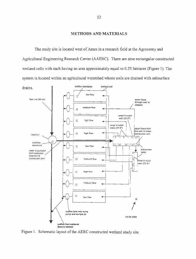
The study site is located west of Ames in a research field at the Agronomy and
Agricultural Engineering Research Center (AAERC). There are nine rectangular constructed
wetland cells with each having an area approximately equal to 0.25 hectares (Figure 1 ). The
system is located within an agricultural watershed whose soils are drained with subsurface
drains .
field tile (30 cm)
reservoir
overflow standpipe
water 1s pumped from collection reservolf to distribution tank
outflow standpipe
low flow 0
medium flow 0
O high flow
0 high flow
0 low flow
0 medium fiow
high flow
medium flow 0
0 low flow
outflow tank with sump pump and sample jar
outflo from wetlands flows to tilemain
wetland cell
water flows through weir to wetland
N
! not to scale
Figure 1. Schematic layout of the AERC constructed wetland study site.

13
Site construction took place during the fall of 1992. Each cell was constructed with
the dimensions represented in Figure 2 with each replication situated as diagrammed in
Figure 3. Each cell has an established cattail stand, Typha glauca, as the dominant emergent
macrophyte. The plants were originally plated at a density of 0.4 rhizomes per square meter
and as of 1998, the density was measured at 50 rhizomes per square meter.
0.9 m ~0.9~
IE-l<-----12.2m ----->~!
Figure 2. Schematic side view of wetland cells.
~N ~3 ~2 ~I ,..---- ----...... ,------- --------- ,.----- ----......
' ,I ' 7 " 7 ' / ' / ' / ' / ' / ' /
116: 1 3491 1046:1 1046: 1 116: 1 349: 1 1046: 1 349: 1 11 6: 1 area area area area area area area area area ratio ratio ratio ratio ratio ratio ratio ratio ratio
42.4 m Cell Cell Cell Cell Cell Cell Cell Cell Cell 9 8 7 6 5 4 3 2 I
I/ ' I/ ' / ' I/
' < 12.2m~ I/ 109.7m ......... ......... /
Figure 3. Overhead schematic of constructed wetland system.
14
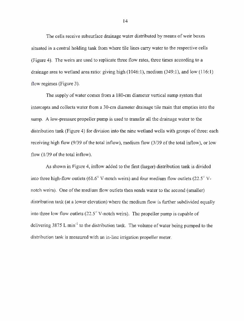
The cells receive subsurface drainage water distributed by means of weir boxes
situated in a central holding tank from where tile lines carry water to the respective cells
(Figure 4). The weirs are used to replicate three flow rates, three times according to a
drainage area to wetland area ratio: giving high (1046:1), medium (349:1), and low (116: 1)
flow regimes (Figure 3).
The supply of water comes from a 180-cm diameter vertical sump system that
intercepts and collects water from a 30-cm diameter drainage tile main that empties into the
sump. A low-pressure propeller pump is used to transfer all the drainage water to the
distribution tank (Figure 4) for division into the nine wetland wells with groups of three: each
receiving high flow (9/39 of the total inflow), medium flow (3/39 of the total inflow), or low
flow (1/39 of the total inflow).
As shown in Figure 4, inflow added to the first (larger) distribution tank is divided
into three high-flow outlets ( 61.6° V-notch weirs) and four medium flow outlets (22.5° V
notch weirs) . One of the medium flow outlets then sends water to the second (smaller)
distribution tank (at a lower elevation) where the medium flow is further subdivided equally
into three low flow outlets (22.5° V-notch weirs). The propeller pump is capable of
delivering 3875 L min-1 to the distribution tank. The volume of water being pumped to the
distribution tank is measured with an in-line irrigation propeller meter.

~ Outlets to Wetland Cells
7l\ O.lm
* Olm
15
1.5 m
Figure 4. Schematics of the distribution tank and 'V' notch weir/boxes.
Each cell has an inlet and outlet tile; the outlet tile being set to maintain a 46-cm
depth of water in each cell. The outlet water is collected in a tank where flow
measurements and water samples are collected (Figure 5). The water is then pumped back
into the main county tile. Specifics of the cells' dimensions and volumes are found in
Table 1.
Tubing
nlet
Figure 5. Outflow collection and sampling diagram
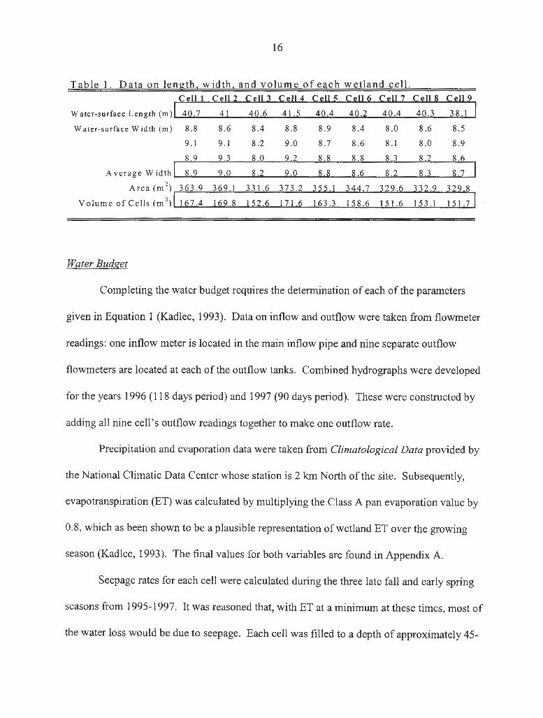
16
Water-surface Length (m)
Water-surface Width (m ) 8 .8 8 .6 8 .4 8 .8 8 .9 8 .4 8.0 8.6 8 .5
9 . 1 9.1 8.2 9.0 8 .7 8.6 8 .1 8.0 8.9
8 .9 9 . ~ 8.Q
::~ ::: 8 .: ::~ 8,2 8 .6
Average Width I 8. 9 9 .0 8 .2 8.3 8 .7 8 .
Area(m 2 ) 363 .9 369 .1 331 .6 373 .2 3 5 5 .1 344.7 329.6 332 .9 329.8
Volume of Cells (m 3)1167.4 169 .8 152.6 171.6 163.3 158.6 151 .6 153 .1 151.71
Water Budget
Completing the water budget requires the determination of each of the parameters
given in Equation 1 (Kadlec, 1993). Data on inflow and outflow were taken from flowmeter
readings: one inflow meter is located in the main inflow pipe and nine separate outflow
flowmeters are located at each of the outflow tanks. Combined hydro graphs were developed
for the years 1996 (118 days period) and 1997 (90 days period). These were constructed by
adding all nine cell's outflow readings together to make one outflow rate.
Precipitation and evaporation data were taken from Climatological Data provided by
the National Climatic Data Center whose station is 2 km North of the site. Subsequently,
evapotranspiration (ET) was calculated by multiplying the Class A pan evaporation value by
0.8, which as been shown to be a plausible representation of wetland ET over the growing
season (Kadlec, 1993). The final values for both variables are found in Appendix A.
Seepage rates for each cell were calculated during the three late fall and early spring
seasons from 1995-1997. It was reasoned that, with ET at a minimum at these times, most of
the water loss would be due to seepage. Each cell was filled to a depth of approximately 45-

17
cm and inlets and outlets were closed off. The change in water levels was recorded twice a
day and rates were calculated from the water level data. In the final water budgets, an overall
average of 0.09 cm/hr was used to represent each cell's seepage rate (Table a.7 in Appendix
A).
Complete water budgets for both years were compiled and consist of each
component's flow values for total inflow and outflow volumes and rates. Outflow:inflow
ratios were determined along with corresponding errors; the error representing the percentage
of total inflow volume that is unaccounted for.
Using the flow data and volume calculations determined in the water budget analyses,
nominal residence times were determined by the equation (Kadlec, 1994):
't = V/Q (2)
Where 't =nominal residence time, day(s); V= total volume of water in the wetland, m3; and
Q = volumetric flow rate, m3 /day. Volumes were calculated using an equation for an earthen
basin (MWPS, 1993).
Where
V = (LW*LL*LD)-(S*LD2)*(LW +LL) + (4*S2*LD3/3) (3)
L W = liquid width, m
LL = liquid length, m
LD = liquid depth, m
S = sideslope, m
Nominal residence times were determined for each flow rate regime, which is to say that an
average of the three replications for each flow rate was calculated to represent each flow
regime (e.g. high, medium, and low). These nominal residence times were then graphed in
comparison with flow rate over time.

18
Tracer Studies
The tracer study was conducted in June 1997, wherein one liter of rhodamine WT
solution with a concentration of 1000 mg/L was introduced as a single pulse into the inlet
pipe of one high flow cell (Cell 6) at the distribution tank. The dose was introduced at night
to minimize photodegradation before the first sampling. The entire cell was roped off into a
grid consisting of forty 4.6 m x 2.1 m rectangles. During each sampling period, samples
were collected at 20-24 random sites in the cell's grid system. A reusable cap for the sample
bottles was fitted with a one-inch head tube to prevent water from simply rushing into the
cap's inflow hole. Instead, the tube allowed the bottle to fill slower as it was lowered into the
cell, thereby obtaining a more depth integrated sample.
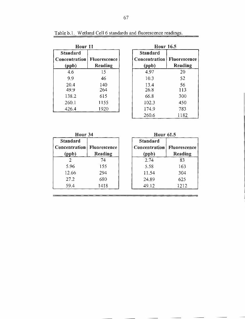
Samples were taken at 11, 16.5, 34, and 61.5 hours post-dosing. In the lab,
standards were developed for each event and each set of sample was analyzed using a Turner
Model 450 digital filter fluorometer. Concentration results can be found in Appendix B
along with the corresponding standard curves and linear regression equations used in
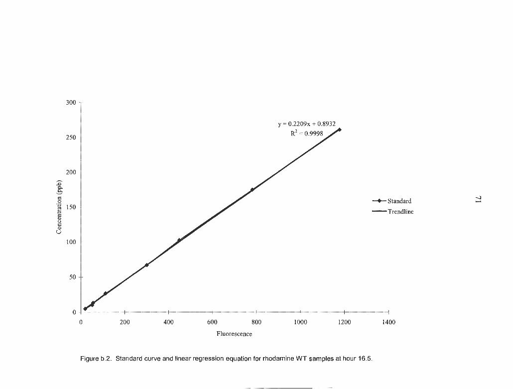
determining sample concentrations. As the graphs show, each event's regression equations
had R-squared values of 0.99, indicating a good correlation. The concentration values were
then mapped into isopleth graphs using the kriging statistical analysis.

19
RESULTS AND DISCUSSION
Water Budget
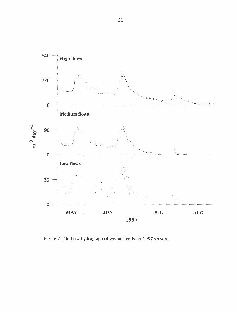
As is evidenced in the hydrographs for each group of flow rates (Figures 6 and 7),
each individual cell of similar flow rate is closely corresponding with the others at its rate.
This lends to giving future studies at the site a good means for proven replication.
The system's 1996 and 1997 combined water budgets (Tables a. l and a.2 in Appendix
A.) were closed within 5.3% and 6.5 % average error, respectively. Such error could possibly
be explained alone by the variability inherent in such 'natural' field studies. However, a
number of other variables more than likely accounted for the error, including: flowmeter
imprecision, the assumption of 0.8 as the ET factor of evaporation, possible berm seepage
and catchment, as well as leaks in the system's piping. Although each is probably not
significant alone, their combined effect may explain the error. Regardless, these errors seem
reasonable for the purposes of closing and modeling the system. Final 1996 and 1997 season
water budgets, by month, are compiled in Tables 2 and 3, respectively. Tables a.3 and a.4 in
Appendix A provide complete water budgets, averaged by treatment, for the three flow
regimes in 1996 and 1997.
The budgets also revealed the significance, if any, of each component's contribution
to the system's total inflow and outflow. Surface inflow and outflow were by far the largest
components of the water budget, followed by seepage, which accounted for 17% and 14% of
the total outflow in 1996 and 1997, respectively. Evapotranspiration was 3.4% of the total

20
540 High flows
270
0 Medium flows
"'"" I
...... 90 ~ "l:I ~
E
0 Low flows
30
0 JUL AUG SEP OCT
1996
Figure 6. Outflow hydrograph of wetland cells for 1996 season.
21
540 l High flows
MAY JUN JUL AUG
1997
Figure 7. Outflow hydrograph of wetland cells for 1997 season.
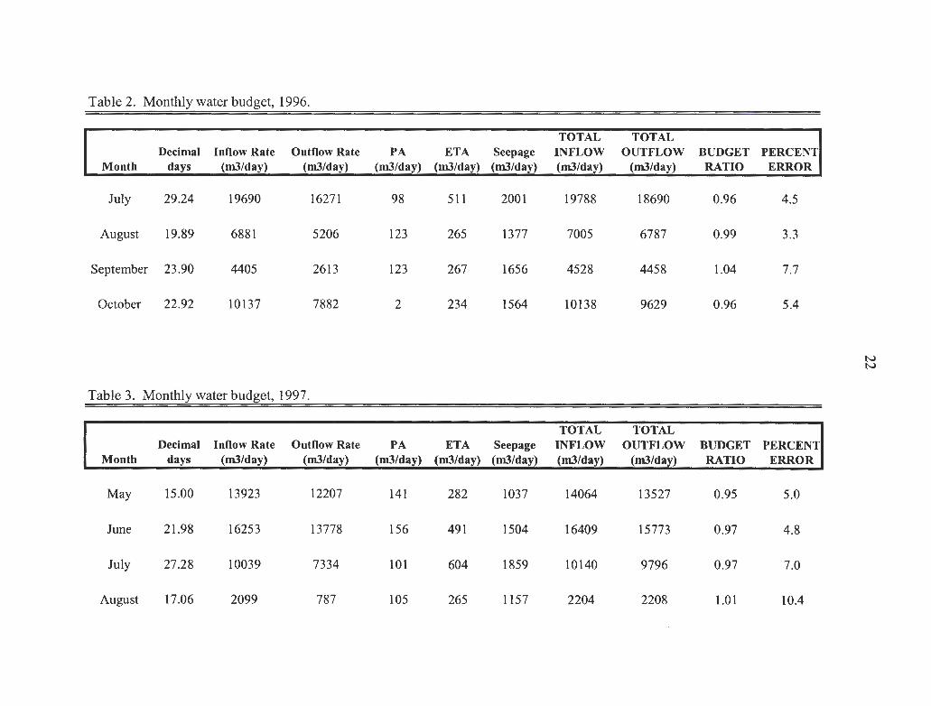
Table 2. Monthly water budget, 1996.
TOTAL TOTAL Decimal Inflow Rate Outflow Rate PA ETA Seepage INFLOW OUTFLOW BUDGET PERCENT
Month days (m3/day) (m3/day) (m3/day) (m3/day) (m3/day) (m3/day) (m3/day) RATIO ERROR
July 29.24 19690 16271 98 511 2001 19788 18690 0.96 4.5
August 19.89 6881 5206 123 265 1377 7005 6787 0.99 3.3
September 23 .90 4405 2613 123 267 1656 4528 4458 1.04 7.7
October 22.92 10137 7882 2 234 1564 10138 9629 0.96 5.4
N N
Table 3. Monthly water budget, 1997.
TOTAL TOTAL Decimal Inflow Rate Outflow Rate PA ETA Seepage INFLOW OUTFLOW BUDGET PERCENT
Month days (m3/day) (m3/day) (m3/day) (m3/day) (m3/day) (m3/day) (m3/day) RATIO ERROR
May 15.00 13923 12207 141 282 1037 14064 13527 0.95 5.0
June 21.98 16253 13778 156 491 1504 16409 15773 0.97 4.8
July 27.28 10039 7334 101 604 1859 10140 9796 0.97 7.0
August 17.06 2099 787 105 265 1157 2204 2208 1.01 10.4

23
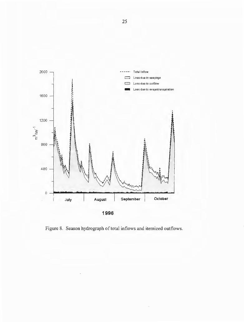
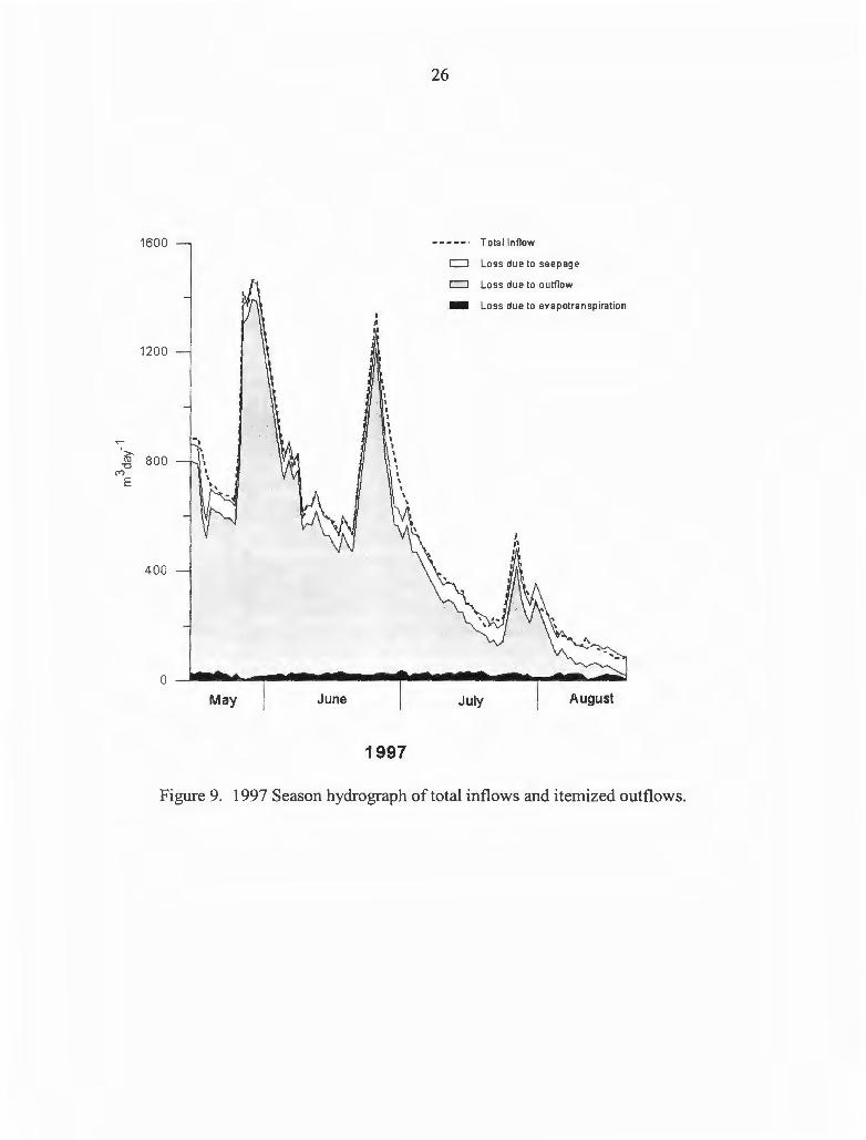
outflow in 1996, and made up 4% of 1997's outflow rate. Precipitation ended up accounting
for 0.8% and 1.2% of the total inflow for the 1996 and 1997 seasons, respectively. This is
demonstrated graphically in Figures 8 and 9, which show that precipitation, ET, and seepage
were minor compared to tile inflow and surface outflow.
In addition to the determination of said hydrologic components, the water budget
outflow data was also used for determining nominal residence times. Daily values of
nominal residence times for 1996 and 1997 can be found in Tables c. l and c.2 in Appendix
C. As these tables show, the average of the daily residence times for each season are as
follows: 1996 averages were 3.6, 29.6, and 106.1 days and 1997 averages were 4.8, 12.1, and
53.0 days for the high, medium, and low flow regimes, respectively. Tables 4 and 5 display
the monthly average flow rates and nominal residence times for each flow regime. Graphing
comparisons (Figures c.1-c.6) show the expected trend where, as flow rate increase the
residence time decreases - and vice versa.
As this study and prior research have shown, outside factors other than surface inflow
and outflow can and do have influence on treatment efficacy and should not be ignored. If at
all possible, they should be quantified and taken into account for any treatment studies
performed in constructed wetlands. This is especially important when using nominal
residence times in model studies. As has been shown, these times are not always true
indicators of actual residence time.
24
Tracer Studies
The rhodamine WT test was only meant to be a small part of the original plans for
tracing the system. The initial plan was to dose the cells with KBr, a conservative tracer,
along with a pesticide (metalachlor) with the rhodamine WT only being used as a visual
tracer. Unfortunately, by the time the potassium bromide was obtained, a dry weather pattern
had reduced inflow rates into the system below the levels considered necessary to properly
model the system.
Being the only mixture in the cocktail available, the dose of rhodamine WT was
introduced before the flow rates dropped too low. Results from the fluorometer readings are
represented by the isopleths in Figure 10. As the dark shape's (higher concentration)
'movement' shows, there is a definite preferential flow path occurring from inlet to outlet.
Note also that the zone to the upper left (SW comer) of the outlet remains at a low
concentration during the entire time, indicating a zone of little or no contact.
This is in concurrence with those findings of Kadlec et al. (1994) and Cooper (1992)
where it has become obvious that constructed wetland systems are indeed dynamic and not
steady state. Therefore, from a modeling standpoint, it would be inappropriate to attempt to
characterize these systems with simple schemes of an ideal reactor. Instead, models of these
wetland systems must be designed so as to take into account the overall flow patterns in the
wetland: described by a number of series and parallel CSTR and PFR.
25
2000 Total Inflow
I CJ Loss due to seepage
I CJ Loss due to outflow
' ' •' •' - Loss due to evapotranspiration
•' 1600 •' •' •' I I I I I I I I I
1200 I I I
~
> ro "O
("")
E . ~
800 I I
'
400
0
July August September October
1996
Figure 8. Season hydrograph of total inflows and itemized outflows.
~
> ro "'O
('<)
E
26
1600 Total Inflow
1200
-' ' 800 1
' 1 \ ,,
400
0
May June
I
' I
•
1 1 1 I 1 1 I 1 1
1 1 \ 1
' '
1997
c:::J Loss due to seepage
CJ Loss due to outflow
- Loss due to evapotranspiration
July August
Figure 9. 1997 Season hydrograph of total inflows and itemized outflows.

27
Table 4. Average of daily flow rates and residence times by month for 1996.
Hieb Flow Medium Flow Low Flow Flow Rate Residence Time Flow Rate Residence Time Flow Rate Residence Time (m3/day) (days) (m3/day) (days) (m3/day) (days)
July 413 1.4 122 5.5 28 29.7
August 199 3.0 47 17.7 11 185.3
September 87 8.4 15 86.6 7 297.7
October 257 2.4 64 12.7 18 42.0
Table 5. Average of daily flow rates and residence times by month for 1997.
Hieb Flow Medium Flow Low Flow Flow Rate Residence Time Flow Rate Residence Time Flow Rate Residence Time
(m3/day) (days) (m3/day) (days) (m3/day) (days) May 606 0.8 176 3.3 55 11.0
June 481 1.0 141 4.0 41 14.6
July 228 2.4 36 21.3 14 93.9
August 43 17.0 No Flow No Flow 2 341.9

11 Hours
N _.
28
16.5 Hours
CJ < IOppb
CJ 10-30ppb
- 40-60ppb
- 70- ll Oppb
- > l lO ppb
34 Hours Inlet
61 .5 Hours
Figure 10. Isopleth of rhodamine WT concentrations over time for Cell 6 tracer study.
29
CONCLUSIONS
With the findings of this research, a better characterization of the hydro logic and
hydrodynamic functions of this site's constructed wetlands was developed. Determining the
relative significance of each component and investigating the flow movements within the
cells provides for important hydrologic data needed for developing water treatment criteria
for all constructed wetlands.
From the water budget, water quality functions such as flow rates and residence times
can be computed, whereby water quality parameters such as loading rates can be assessed.
The rhodamine WT tracer study conducted was only a glimpse at what hydrodynamics are
occurring in these cells. Other flow rates under varying environmental conditions must also
be studied before any formidable conclusions can be made about such treatment systems.
However, this tracer dose did show that the flow paths within the wetland system are not
uniform and could have serious impacts in accurately predicting the system's treatment
efficiency. If not properly regarded, the preferential flow paths and areas of little or no
contact which prevail in these non-ideal reactors could lead to serious errors in treatment
criteria; resulting in under- or over-designed constructed wetland systems.
Future tracer tests will provide a more thorough look into the hydrodynamics
associated within constructed wetlands. Furthermore, such tracer studies will allow for the
comparison of the discrepancies between nominal residence times versus actual residence
times. Overall, knowing the significance of the hydrologic components as well as the

30
hydrodynamic flows will provide for better information on the variables required to more
accurately model treatment capabilities and efficiency potentials.

31
APPENDIX A
HYDROLOGY DATA
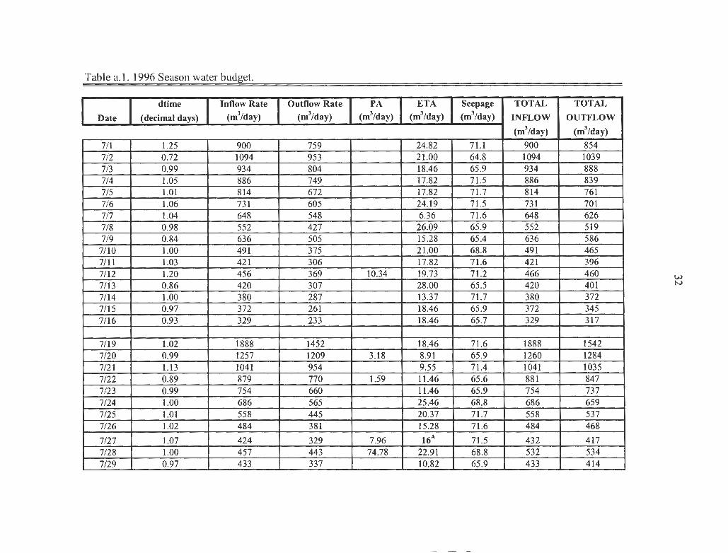
Table a. l. 1996 Season water budget.
dtime Inflow Rate Outflow Rate PA
Date (decimal days) (m3/day) (m3/day) (m3/day)
7/1 1.25 900 759 7/2 0.72 1094 953 7/3 0.99 934 804 7/4 1.05 886 749 7/5 1.01 814 672 716 1.06 731 605 7/7 1.04 648 548 7/8 0.98 552 427 7/9 0.84 636 505
7/10 1.00 491 375 7/11 1.03 421 306 7/12 1.20 456 369 10.34 7113 0.86 420 307 7/14 1.00 380 287 7/15 0.97 372 261 7/16 0.93 329 233
7/19 1.02 1888 1452 7/20 0.99 1257 1209 3.18 7/21 1.13 1041 954 7/22 0.89 879 770 1.59 7/23 0.99 754 660 7/24 1.00 686 565 7/25 1.01 558 445 7/26 1.02 484 381
7/27 1.07 424 329 7.96 7/28 1.00 457 443 74.78 7/29 0.97 433 337
ETA Seepage
(m3/day) (m3/day)
24.82 71.1 21.00 64.8 18.46 65.9 17.82 71.5 17.82 71.7 24.19 71.5 6.36 71.6
26.09 65.9 15.28 65.4 21.00 68.8 17.82 71.6 19.73 71.2 28.00 65.5 13.37 71.7 18.46 65.9 18.46 65.7
18.46 71.6 8.91 65.9 9.55 71.4 11.46 65.6 11.46 65.9 25.46 68.8 20.37 71.7 15.28 71.6 16A 71.5
22.91 68.8 10.82 65.9
TOTAL
INFLOW
(m3/day)
900 1094 934 886 814 731 648 552 636 491 421 466 420 380 372 329
1888 1260 1041 881 754 686 558 484
432 532 433
TOTAL
OUTFLOW
(m3/day)
854 1039 888 839 761 701 626 519 586 465 396 460 401 372 345 317
1542 1284 1035 847 737 659 537 468
417 534 414
w N
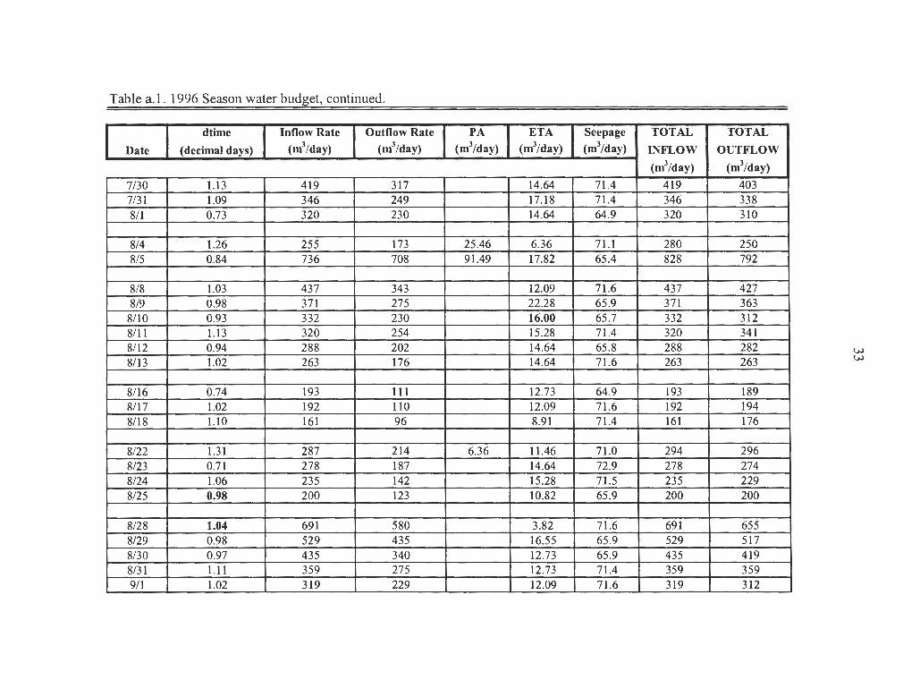
Table a. l . 1996 Season water budget, continued.
dtime Inflow Rate Outflow Rate PA
Date (decimal days) (m3/day) (m3/day) (m3/day)
7/30 1.13 419 317 7/31 1.09 346 249 8/1 0.73 320 230
8/4 1.26 255 173 25.46 8/5 0.84 736 708 91.49
8/8 1.03 437 343 8/9 0.98 371 275 8/10 0.93 332 230 8/11 1.13 320 254 8/12 0.94 288 202 8/13 1.02 263 176
8/16 0.74 193 111 8/17 1.02 192 110 8/18 1.10 161 96
8/22 1.31 287 214 6.36 8/23 0.71 278 187 8/24 1.06 235 142 8/25 0.98 200 123
8/28 1.04 691 580 8/29 0.98 529 435 8/30 0.97 435 340 8/31 1.11 359 275 9/1 1.02 319 229
ETA Seepage
(m3/day) (m3/day)
14.64 71.4 17.18 71.4 14.64 64.9
6.36 71.1 17.82 65.4
12.09 71.6 22.28 65.9 16.00 65.7 15.28 71.4 14.64 65 .8 14.64 71.6
12.73 64.9 12.09 71.6 8.91 71.4
11.46 71.0 14.64 72.9 15.28 71.5 10.82 65.9
3.82 71.6 16.55 65.9 12.73 65 .9 12.73 71.4 12.09 71.6
TOTAL
INFLOW
(m3/day)
419 346 320
280 828
437 371 332 320 288 263
193 192 161
294 278 235 200
691 529 435 359 319
TOTAL
OUTFLOW
(m3/day)
403 338 310
250 792
427 363 312 341 282 263
189 194 176
296 274 229 200
655 517 419 359 312
l>J l>J

Table a.1. 1996 Season water budget, continued.
dtime Inflow Rate Outflow Rate PA
Date (decimal days) (m3/day) (m3/day) (m3/day)
912 0.98 276 187 9/3 1.05 239 153 9/4 0.94 210 128 915 1.04 205 111 916 0.97 165 90 917 1.04 154 86 9/8 1.10 161 108 44.55 919 0.89 161 94 9/ 10 1.03 155 76 9/11 0.98 145 69 9/12 1.02 122 63 9/13 0.88 161 73 9/14 1.00 113 47 9/15 1.23 108 47
9/18 0.97 98 37 9119 1.02 112 35 9120 1.06 89 52 32.62 9121 0.86 110 34 9/22 1.05 90 32 9/23 1.08 88 44 40.57 9/24 0.98 116 39 9125 0.89 108 39 5.57
9/28 0.81 900 742
10/2 1.04 496 388 10/3 0.90 418 329
ETA Seepage TOTAL
(m3/day) (m3/day) INFLOW
(m3/day)
16.55 65 .9 276 14.00 71.5 239 9.55 65 .8 210 16.55 71.6 205 17.18 65 .9 165 13.37 71.6 154 10.18 71.4 206 3.18 65.6 161 9.55 71.6 155 17.82 65.9 145 11.46 71.6 122 3.82 65.5 161 10.18 68.8 113 17.82 71.2 108
10.18 65 .9 98 9.55 71.6 112 13.37 71.5 122 7.00 65.5 110 7.64 71.5 90 8.27 71.5 128 8.27 71.7 116 5.73 65.6 113
13 .37 65 .3 900
14.64 71.6 496 9.55 65.6 418
--- ----~-
TOTAL
OUTFLOW
(m3/day)
269 238 204 200 173 171 190 163 157 152 146 142 126 136
113 116 137 106 111 124 119 110
820
474 404
w ~

Table a.1. 1996 Season water budget, continued.
dtime Inflow Rate Outflow Rate PA
Date (decimal days) (m3/day) (m3/day) (m3/day)
10/4 1.03 440 334 10/5 1.22 419 315 10/6 0.89 398 298 10/7 0.97 363 279 10/8 0.92 363 268 10/9 1.05 353 268 1.59
10/10 0.91 341 232 10/ 11 0.99 355 265 10/12 1.27 275 204 10/13 0.73 426 289 10/14 1.14 205 145 10115 1.00 290 189 10/16 0.99 294 190 10/17 0.88 300 211 10/18 0.97 248 175 10/19 1.03 262 165 10/20 1.30 267 170 10/21 0.76 228 157
10/25 0.89 1363 1234 10/26 1.07 1109 970 10/27 0.99 924 807
A Bold face indicates estimated time.
ETA Seepage
(m3/day) (m3/day)
8.27 71.6 12.09 71.2 7.64 65.6 10.18 65 .9 4.46 65.7 12.09 71.5 8.27 65 .7 10.82 65 .9 8.27 71.1 6.36 64.9 14.00 71.3 12.73 68.8 8.27 65.9 8.91 65.5 11.46 65.9 14.64 71.6 22.28 71.0 1.91 65.0
7.00 65 .6 7.64 71.5 12.73 65 .9
TOTAL
INFLOW
(m3/day)
440 419 398 363 363 355 341 355 275 426 205 290 294 300 248 262 267 228
1363 1109 924
TOTAL
OUTFLOW
(m3/day)
414 399 371 355 339 351 306 342 283 360 231 270 264 285 253 251 264 224
1307 1049 885
w Vl
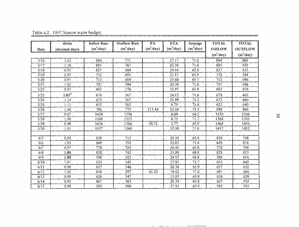
Table a.2. 1997 Season water budget.
dtime Inflow Rate Outflow Rate PA
Date (decimal days) (m3/day) (m3/day) (m3/day)
5116 1.03 884 771 5/17 1.10 885 767 5/18 0.95 827 560 5119 0.97 752 491 5120 0.91 712 604 5/21 1.02 707 594 5122 0.97 683 576
5123 1.03A 678 567 5124 1.14 672 567 5125 1.11 652 562 5/26 1.06 786 775 111.44 5127 0.67 1420 1296 5/28 1.00 1368 1323 5129 0.99 1438 1386 29.72 5/30 1.05 1457 1369
615 0.95 828 712 616 1.03 849 792 617 0.97 778 705 6/8 1.00 828 742 619 1.00 588 523
6110 1.01 635 542 6/11 0.98 637 546 6/12 1.02 630 597 61.29 6/13 0.99 626 547 6/14 0.95 607 505 6/15 0.98 585 500
ETA Seepage
(m3/day) (m3/day)
27.17 71.6 20.38 71.4 29.44 65 .8 27.17 65.9 25 .66 65.7 20.38 71.6 33.97 65 .9
24.15 71.6 21.89 71.3 6.79 71.4
22.64 71.5 6.04 64.5 0.75 71.7 3.77 65.9 12.08 71.6
20.38 65.8 12.83 71.6 26.42 65 .8 21.89 68.8 24.15 68.8 27.93 71.7 20.38 65.9 19.62 71.6 15.85 65.9 20.38 65.8 27.93 65.9
TOTAL
INFLOW
(m3/day)
884 885 827 752 712 707 683
678 672 652 898 1420 1368 1468 1457
828 849 778 828 588 635 637 691 626 607 585
TOTAL
OUTFLOW
(m3/day)
869 859 655 584 696 686 676
662 660 640 869 1366 1395 1456 1452
798 876 798 833 616 642 632 688 629 592 593
\.;.)
0\
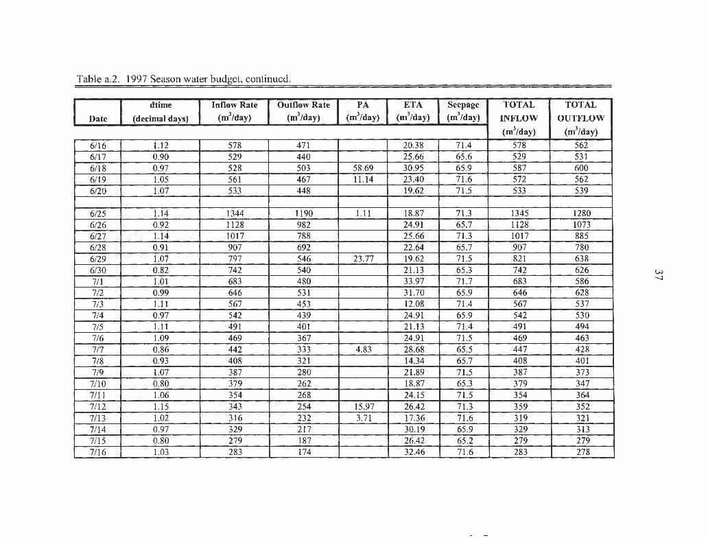
Table a.2. 1997 Season water budget, continued.
dtime Inflow Rate Outflow Rate PA
Date (decimal days) (m3/day) (m3/day) (m3/day)
6/16 1.12 578 471 6/17 0.90 529 440 6/18 0.97 528 503 58.69 6/19 1.05 561 467 11.14 6120 1.07 533 448
6125 1.14 1344 1190 1.11 6126 0.92 1128 982 6/27 1.14 1017 788 6/28 0.91 907 692 6129 1.07 797 546 23.77 6/30 0.82 742 540 7/1 1.01 683 480 7/2 0.99 646 531 7/3 1.11 567 453 7/4 0.97 542 439 7/5 1.11 491 401 7/6 1.09 469 367 7/7 0.86 442 333 4.83 7/8 0.93 408 321 7/9 1.07 387 280 7/10 0.80 379 262 7/11 1.06 354 268 7/12 1.15 343 254 15.97 7/13 1.02 316 232 3.71 7/14 0.97 329 217 7/15 0.80 279 187 7/16 1.03 283 174
ETA Seepage
(m3/day) (m3/day)
20.38 71.4 25.66 65.6 30.95 65.9 23.40 71.6 19.62 71.5
18.87 71.3 24.91 65.7 25.66 71.3 22.64 65.7 19.62 71.5 21.13 65.3 33.97 71.7 31 .70 65.9 12.08 71.4 24.91 65.9 21.13 71.4 24.91 71.5 28.68 65.5 14.34 65.7 21.89 71.5 18.87 65.3 24.15 71.5 26.42 71.3 17.36 71.6 30.19 65.9 26.42 65.2 32.46 71.6
TOTAL
INFLOW
(m3/day)
578 529 587 572 533
1345 1128 1017 907 821 742 683 646 567 542 491 469 447 408 387 379 354 359 319 329 279 283
TOTAL
OUTFLOW
(m3/day)
562 531 600 562 539
1280 1073 885 780 638 626 586 628 537 530 494 463 428 401 373 347 364 352 321 313 279 278
VJ -...)

Table a.2. 1997 Season water budget, continued.
dtime Inflow Rate Outflow Rate PA
Date (decimal days) (m3/day) (m3/day) (m3/day)
7/17 1.01 248 161 2.23
7/19 1.35 195 132 7/20 0.87 202 117 1.86 7/21 0.77 206 133 28.23 7/22 0.94 219 111 7/23 1.16 198 122 33.80
7126 0.96 539 387 7/27 1.10 394 274 10.77 7/28 0.91 333 229 7/29 1.04 307 189 7/30 1.19 282 279
8/3 1.01 225 113 8/4 1.00 174 69 8/5 1.06 165 90 8/6 1.33 158 65 8/7 0.68 153 60 8/8 0.94 129 38 8/9 1.11 126 40
8/10 1.26 97 31 61.29 8/11 0.82 127 54 8/12 0.88 99 60 31 .20 8/13 0.94 112 51 2.23 8/14 0.99 105 30 8/15 0.98 107 36
ETA Seepage
(m3/day) (m3/day)
23.40 71.7
31.70 70.9 20.38 65.5 12.83 65.1 14.34 65.8 17.36 71.3
25.66 65.8 22.64 71.4 15.85 65.7 19.62 71.6 10.57 71.2
10.57 71.7 20.38 68.8 26.42 71.5 15.10 71.0 22.64 64.6 22.64 65.8 22.64 71.4 17.36 71.1 2.26 65.3 3.02 65.6 9.06 65.8 15.85 65.9 19.62 65.9
TOTAL
INFLOW
(m3/day)
250
195 204 234 219 232
539 405 333 307 282
225 174 165 158 153 129 126 158 127 130 114 105 107
TOTAL
OUTFLOW
(m3/day)
256
234 202 211 191 211
478 368 310 280 361
195 158 188 151 147 126 134 120 122 129 125 111 121
w 00

Table a.2. 1997 Season water budget, continued.
dtime Inflow Rate Outflow Rate PA
Date (decimal days) (m3/day) (m3/day) (m3/day)
8/ 16 1.45 84 20 8/17 1.07 81 10 8/18 0.86 80 10 8/ 19 0.68 77 12 10.40
A Bold face indicates estimated time.
ETA Seepage
(m3/day) (m3/day)
18.87 70.8 18.12 71.5 12.83 65.5 7.55 64.6
TOTAL
INFLOW
(m3/day)
84 81 80 87
TOTAL
OUTFLOW
(m3/day)
110 100 88 84
w
'°

40
Table a.3. 1996 Season flowmeter measurements by flow regime.
Main Inflow Low Outflow Med Outflow High Outflow
DATE m3/day m3/day m3/day m3/day
1-Jul 900 30 170 559 2-Jul 1094 37 211 705 3-Jul 934 31 178 595 4-Jul 886 35 168 549 5-Jul 814 35 148 489 6-Jul 731 28 131 446 7-Jul 648 26 118 403 8-Jul 552 17 91 319 9-Jul 636 16 105 384 10-Jul 491 14 76 285 11-Jul 421 10 59 237
13-Jul 420 9 59 239 14-Jul 380 8 55 225 15-Jul 372 7 49 205 16-Jul 329 5 42 185
19-Jul 1888 122 401 928 20-Jul 1257 73 254 883 21-Jul 1041 60 215 679 22-Jul 879 43 170 556 23-Jul 754 36 141 483 24-Jul 686 25 119 421 25-Jul 558 17 89 338 26-Jul 484 14 75 292 27-Jul 424 14 64 251 28-Jul 457 43 98 302 29-Jul 433 15 66 256 30-Jul 419 13 60 245 31-Jul 346 7 45 197 1-Aug 320 6 41 184
4-Aug 255 3 26 148 5-Aug 736 60 164 485

41
Table a.3. 1996 Season flowmeter measurements by flow regime (continued).
Main Inflow Low Outflow Med Outflow High Outflow
DATE m3/day m3/day m3/day m3/day
11-Aug 320 12 46 196 12-Aug 288 8 33 161 13-Aug 263 7 27 142
16-Aug 193 1 13 97 17-Aug 192 1 14 95 18-Aug 161 0 10 86
22-Aug 287 7 38 168 23-Aug 278 7 33 147 24-Aug 235 3 19 120 25-Aug 200 1 16 106
28-Aug 691 29 127 424 29-Aug 529 20 89 326 30-Aug 435 14 66 261 31-Aug 359 10 51 214 1-Sep 319 8 41 180 2-Sep 276 6 32 149 3-Sep 239 4 22 127 4-Sep 210 3 17 108 5-Sep 205 2 13 97 6-Sep 165 1 9 79 7-Sep 154 0 9 76 8-Sep 161 4 18 91 9-Sep 161 3 11 80 10-Sep 155 1 7 68 11-Sep 145 0 6 63 12-Sep 122 0 5 57 13-Sep 161 0 7 66 14-Sep 113 0 4 43 15-Sep 108 0 4 43
18-Sep 98 0 3 34

42
Table a.3. 1996 Season flowmeter measurements by flow regime (continued).
Main Inflow Low Outflow Med Outflow High Outflow
DATE m3/day m3/day m3/day m3/day
19-Sep 112 0 3 32
23-Sep 88 0 6 39 24-Sep 116 0 4 35 25-Sep 108 0 3 35
28-Sep 900 54 163 572
2-0ct 496 19 73 295 3-0ct 418 19 57 253 4-0ct 440 15 61 258 5-0ct 419 14 56 245 6-0ct 398 17 51 230 7-0ct 363 14 48 218 8-0ct 363 13 44 211 9-0ct 353 12 45 210 10-0ct 341 12 38 182 11-0ct 355 11 40 214 12-0ct 275 IO 32 163 13-0ct 426 14 44 231 14-0ct 205 8 24 121 15-0ct 290 8 32 159 16-0ct 294 8 27 154 17-0ct 300 10 34 167 18-0ct 248 8 27 141 19-0ct 262 6 22 138 20-0ct 267 6 25 140 21-0ct 228 9 22 125
25-0ct 1363 92 284 859 26-0ct 1109 53 221 696 27-0ct 924 47 179 581
Average 441 17 69 259 Total Flow 38216 1459 5968 22493

43
Table a.4. 1997 Season flowmeter measurements by flow regime.
Main Inflow Low Outflow Med Outflow High Outflow
DATE m3/day m3/day m3/day m3/day
16-May 884 43 158 570 17-May 885 43 160 565 18-May 827 42 152 549 19-May 752 34 130 490 20-May 712 33 120 452 21 -May 707 35 116 442 22-May 683 28 113 435 23-May 678 30 111 426 24-May 672 34 114 419 25-May 652 32 112 418 26-May 786 69 173 533 27-May 1420 94 287 915 28-May 1368 99 289 935 29-May 1438 105 305 976 30-May 1457 99 298 970
5-Jun 828 40 142 531 6-Jun 849 47 163 581 7-Jun 778 41 143 521 8-Jun 828 41 148 553 9-Jun 588 28 101 394 10-Jun 635 28 105 409 11-Jun 637 30 104 412 12-Jun 630 44 128 424 13-Jun 626 31 107 409 14-Jun 607 27 96 383 15-Jun 585 25 102 372 16-Jun 578 25 78 368 17-Jun 529 18 88 334 18-Jun 528 35 106 362 19-Jun 561 16 91 360 20-Jun 533 23 85 340
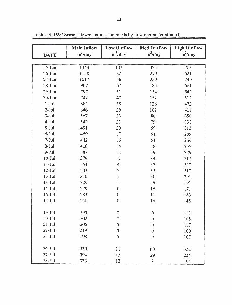
44
Table a.4. 1997 Season flowmeter measurements by flow regime (continued).
Main Inflow Low Outflow Med Outflow High Outflow
DATE m3/day m3/day m3/day m3/day
25-Jun 1344 103 324 763 26-Jun 1128 82 279 621 27-Jun 1017 66 229 740 28-Jun 907 67 184 661 29-Jun 797 31 154 542 30-Jun 742 47 152 512 1-Jul 683 38 128 472 2-Jul 646 29 102 401 3-Jul 567 23 80 350 4-Jul 542 23 79 338 5-Jul 491 20 69 312 6-Jul 469 17 61 289 7-Jul 442 16 51 266 8-Jul 408 16 48 257 9-Jul 387 12 39 229 10-Jul 379 12 34 217 11-Jul 354 4 37 227 12-Jul 343 2 35 217 13-Jul 316 1 30 201 14-Jul 329 1 25 191 15-Jul 279 0 16 171 16-Jul 283 0 11 163 17-Jul 248 0 16 145
19-Jul 195 0 0 123 20-Jul 202 0 0 108 21-Jul 206 5 0 117 22-Jul 219 3 0 100 23-Jul 198 5 0 107
26-Jul 539 21 60 322 27-Jul 394 13 29 224 28-Jul 333 12 8 194

45
Table a.4. 1997 Season flowmeter measurements by flow regime (continued).
Main Inflow Low Outflow Med Outflow High Outflow
DATE m3/day m3/day m3/day m3/day
29-Jul 307 7 6 165
30-Jul 282 7 3 249
3-Aug 225 2 0 103 4-Aug 174 1 0 61 5-Aug 165 0 0 86 6-Aug 158 0 0 62 7-Aug 153 0 0 57 8-Aug 129 0 0 36 9-Aug 126 0 0 38 10-Aug 97 0 0 30 11-Aug 127 0 0 51 12-Aug 99 0 0 54 13-Aug 112 0 0 47 14-Aug 105 0 0 28 15-Aug 107 0 0 34 16-Aug 84 0 0 19 17-Aug 81 0 0 10 18-Aug 80 0 0 10 19-Aug 77 0 0 12
Average 522 25 83 328 Total Flow 42314 2006 6712 26581

46
Table a.5. 1996 Flow ratios and error.
TOTAL TOTAL INFLOW OUTFLOW BUDGET PERCENT
DATE (m3/day) (m3/day) RATIO ERROR 711 900 854 0.95 5.1 7/2 1094 1039 0.95 5.0 7/3 934 888 0.95 5.0 7/4 886 839 0.95 5.3 715 814 761 0.93 6.5 7/6 731 701 0.96 4.1 7/7 648 626 0.97 3.4 7/8 552 519 0.94 6.0 719 636 586 0.92 7.9
7110 491 465 0.95 5.4 7/11 421 396 0.94 6.1 7/12 466 460 0.99 1.3 7/13 420 401 0.95 4.6 7/14 380 372 0.98 1.9 7/15 372 345 0.93 7.2 7/16 329 317 0.96 3.8
7/19 1888 1542 0.82 18.3 7/20 1260 1284 1.02 1.9 7/21 1041 1035 0.99 0.6 7/22 881 847 0.96 3.8 7/23 754 737 0.98 2.3 7/24 686 659 0.96 4.0 7/25 558 537 0.96 3.8 7/26 484 468 0.97 3.4 7/27 432 417 0.97 3.5 7/28 532 534 1.01 0.5 7/29 433 414 0.96 4.4 7/30 419 403 0.96 3.7 7/31 346 338 0.98 2.2 8/1 320 310 0.97 3.1
8/4 280 250 0.89 10.8 8/5 828 792 0.96 4.3
8/8 437 427 0.98 2.2 8/9 371 363 0.98 2.1 8/10 332 312 0.94 5.9 8/11 320 341 1.06 6.4 8/12 288 282 0.98 1.9 8/13 263 263 1.00 0.2

47
Table a.5. 1996 Flow ratios and error, continued.
TOTAL TOTAL INFLOW OUTFLOW BUDGET PERCENT
DATE (m3/day) (m3/day) RATIO ERROR 8/16 193 189 0.98 2.2 8/17 192 194 1.01 1.2 8/18 161 176 1.09 9.5
8/22 294 296 1.01 0.8 8/23 278 274 0.99 1.5 8/24 235 229 0.97 2.5 8/25 200 200 1.00 0.0
8/28 691 655 0.95 5.2 8/29 529 517 0.98 2.3 8/30 435 419 0.96 3.6 8/3 1 359 359 1.00 0.2 911 319 312 0.98 2.1 912 276 269 0.98 2.3 9/3 239 238 1.00 0.2 914 210 204 0.97 3.0 915 205 200 0.97 2.8 916 165 173 1.05 4.6 917 154 171 1.11 11.0 9/8 206 190 0.92 7.6 919 161 163 1.01 1.2 9/10 155 157 1.01 1.3 9/11 145 152 1.05 4.8 9112 122 146 1.19 19.5 9/13 161 142 0.88 11.9 9/14 113 126 1.12 11.7 9/15 108 136 1.26 25 .7
9/18 98 113 1.15 15.2 9119 112 116 1.04 3.5 9120 122 137 1.12 12.0 9/21 110 106 0.97 3.4 9122 90 111 1.23 22.9 9123 128 124 0.97 3.3 9/24 116 119 1.02 2.4 9/25 113 110 0.97 3.0
9/28 900 820 0.91 8.8
10/2 496 474 0.96 4.5 10/3 418 404 0.97 3.5
48
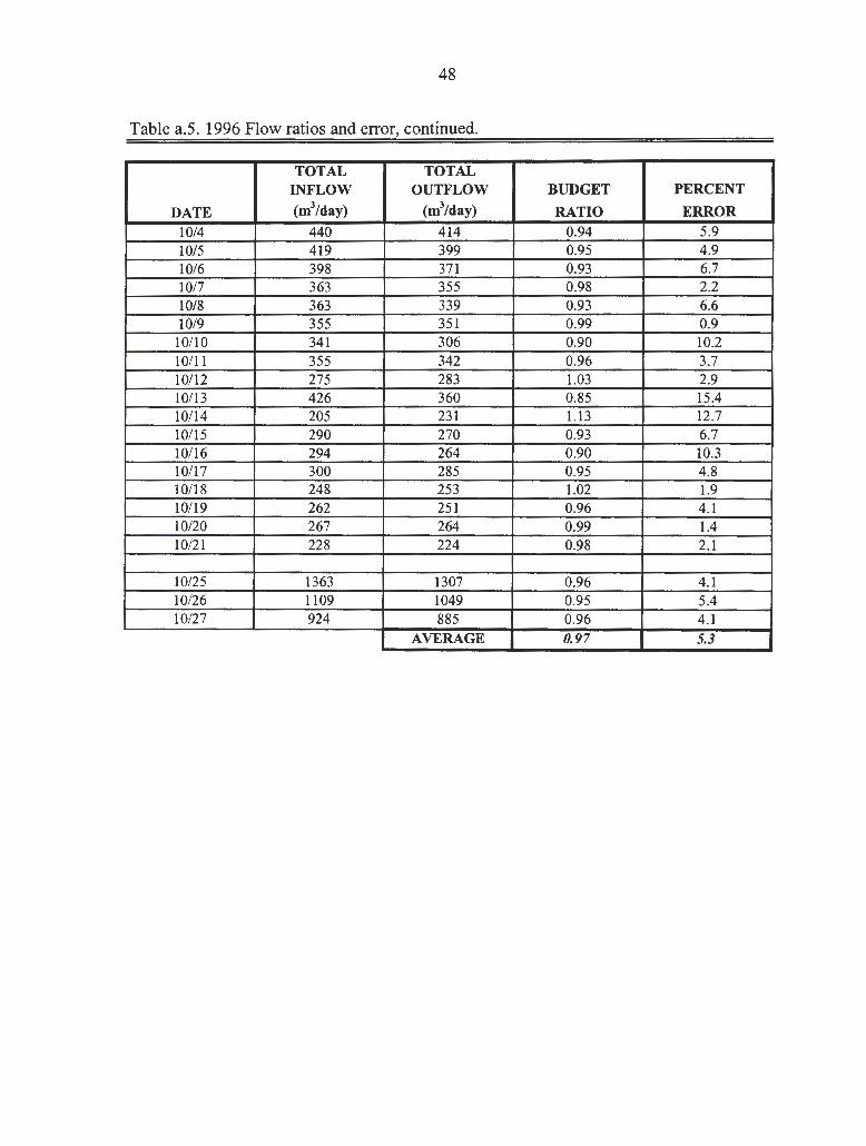
Table a.5. 1996 Flow ratios and error, continued.
TOTAL TOTAL INFLOW OUTFLOW BUDGET PERCENT
DATE (m3/day) (m3/day) RATIO ERROR 1014 440 414 0.94 5.9 1015 419 399 0.95 4.9 10/6 398 371 0.93 6.7 1017 363 355 0.98 2.2 10/8 363 339 0.93 6.6 10/9 355 351 0.99 0.9
10/10 341 306 0.90 10.2 10/11 355 342 0.96 3.7 10/12 275 283 1.03 2.9 10/13 426 360 0.85 15.4 10/14 205 231 1.13 12.7 10115 290 270 0.93 6.7 10/16 294 264 0.90 10.3 10/17 300 285 0.95 4.8 10/18 248 253 1.02 1.9 10/19 262 251 0.96 4.1 10/20 267 264 0.99 1.4 10/21 228 224 0.98 2.1
10/25 1363 1307 0.96 4.1 10/26 1109 1049 0.95 5.4 10/27 924 885 0.96 4.1
AVERAGE 0.97 5.3
49
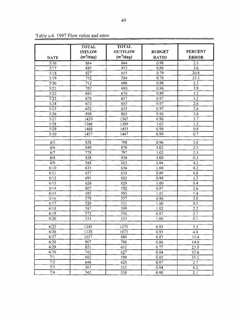
Table a.6. 1997 Flow ratios and error.
TOTAL TOTAL INFLOW OUTFLOW BUDGET PERCENT
DATE (m3/day) (m3/day) RATIO ERROR 5/16 884 864 0.98 2.3 5/17 885 853 0.96 3.6 5118 827 655 0.79 20.8 5/19 752 584 0.78 22.3 5120 712 696 0.98 2.3 5/21 707 680 0.96 3.9 5122 683 676 0.99 1.2 5/23 678 657 0.97 3.2 5/24 672 655 0.97 2.6 5125 652 635 0.97 2.6 5126 898 863 0.96 3.8 5/27 1420 1367 0.96 3.7 5/28 1368 1389 1.02 1.5
5129 1468 1455 0.99 0.8 5/30 1457 1447 0.99 0.7
615 828 798 0.96 3.6 616 849 870 1.02 2.5 617 778 797 1.03 2.5 6/8 828 830 1.00 0.3 619 588 613 1.04 4.3 6/10 635 636 1.00 0.2 6/11 637 632 0.99 0.8 6112 691 682 0.99 1.2 6/13 626 629 1.00 0.4 6/14 607 592 0.97 2.6 6115 585 593 1.01 1.4 6/16 578 557 0.96 3.8 6117 529 531 1.00 0.5 6118 587 599 1.02 2.2 6/19 572 556 0.97 2.7 6120 533 533 1.00 0.1
6125 1345 1275 0.95 5.2 6126 1128 1073 0.95 4.9 6/27 1017 880 0.87 13.4 6/28 907 780 0.86 14.0 6129 821 632 0.77 23.0 6130 742 627 0.84 15.6 7/1 683 580 0.85 15.1 7/2 646 628 0.97 2.7 7/3 567 531 0.94 6.2 7/4 542 530 0.98 2.1
50
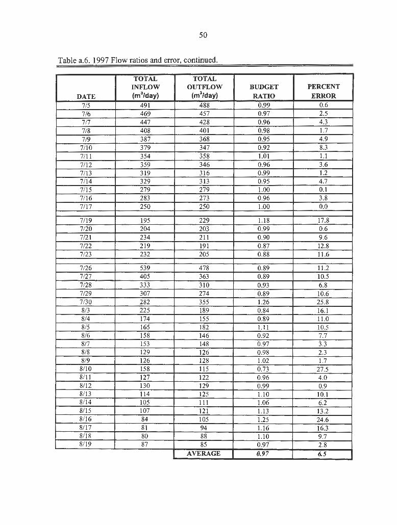
Table a.6. 1997 Flow ratios and error, continued.
TOTAL TOTAL INFLOW OUTFLOW BUDGET PERCENT
DATE (m3/day) (m3/day) RATIO ERROR 715 491 488 0.99 0.6 716 469 457 0.97 2.5 7/7 447 428 0.96 4.3 7/8 408 401 0.98 1.7 7/9 387 368 0.95 4.9 7/10 379 347 0.92 8.3 7/11 354 358 1.01 1.1 7112 359 346 0.96 3.6 7/13 319 316 0.99 1.2 7/14 329 313 0.95 4.7 7/15 279 279 1.00 0.1 7/16 283 273 0.96 3.8 7/17 250 250 1.00 0.0
7/19 195 229 1.18 17.8 7/20 204 203 0.99 0.6 7/21 234 211 0.90 9.6 7/22 219 191 0.87 12.8 7/23 232 205 0.88 11.6
7/26 539 478 0.89 11.2 7/27 405 363 0.89 10.5 7/28 333 310 0.93 6.8 7/29 307 274 0.89 10.6 7/30 282 355 1.26 25.8 8/3 225 189 0.84 16.1 8/4 174 155 0.89 11.0 8/5 165 182 1.11 10.5 8/6 158 146 0.92 7.7 8/7 153 148 0.97 3.3 8/8 129 126 0.98 2.3 8/9 126 128 1.02 1.7 8/10 158 115 0.73 27.5 8/11 127 122 0.96 4.0 8/12 130 129 0.99 0.9 8/13 114 125 1.10 10.1 8/14 105 111 1.06 6.2 8/15 107 121 1.13 13.2 8/16 84 105 1.25 24.6 8/17 81 94 1.16 16.3 8/18 80 88 1.10 9.7 8/19 87 85 0.97 2.8
AVERAGE 0.97 6.5
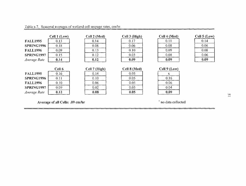
Table a. 7. Seasonal averages of wetland cell seepage rates, cm/hr.
Cell 1 (Low) Cell 2 (Med) Cell 3 (High) Cell 4 (Med) Cell 5 (Low) FALL1995 0.13 0.14 0.17 0.11 0.14 SPRING1996 0.18 0.08 0.06 0.08 0.06 FALL1996 0.09 0.13 0.10 0.09 0.08 SPRING1997 0.15 0.12 0.03 0.08 0.06 Average Rate 0.14 0.12 0.09 0.09 0.09
Cell 6 Cell 7 (High) Cell 8 (Med) Cell 9 (Low) FALL1995 0.16 0.14 0.05 x SPRING1996 0.11 0.10 0.05 0.16 FALL1996 0.10 0.06 0.05 0.06 SPRING1997 0.09 0.02 0.03 0.04 Average Rate 0.12 0.08 0.05 0.09
VI -Average of all Cells: .09 cm/hr x no data collected
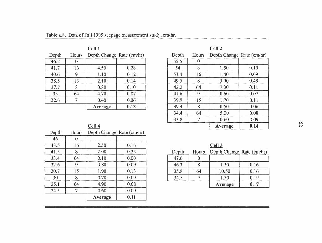
Table a.8. Data of Fall 1995 seepage measurement study, cm/hr.
Cell 1 Cell 2 Depth Hours Depth Change Rate (cm/hr) Depth Hours Depth Change Rate (cm/hr) - - -46.2 0 55.5 0 41.7 16 4.50 0.28 54 8 1.50 0.19 40.6 9 1.10 0.12 53.4 16 1.40 0.09 38.5 15 2.10 0.14 49.5 8 3.90 0.49 37.7 8 0.80 0.10 42.2 64 7.30 0.11 33 64 4.70 0.07 41.6 9 0.60 0.07
32.6 7 0.40 0.06 39.9 15 1.70 0.11 Average 0.13 39.4 8 0.50 0.06
34.4 64 5.00 0.08 33.8 7 0.60 0.09
Cell 4 Average 0.14 Depth Hours Depth Change Rate (cm/hr)
46 0 43.5 16 2.50 0.16 Cell 3 41.5 8 2.00 0.25 Depth Hours Depth Change Rate (cm/hr) 33.4 64 0.10 0.00 47.6 0 32.6 9 0.80 0.09 46.3 8 1.30 0.16 30.7 15 1.90 0.13 35.8 64 10.50 0.16 30 8 0.70 0.09 34.5 7 1.30 0.19
25.l 64 4.90 0.08 Average 0.17 24.5 7 0.60 0.09
Average 0.11
Vl N

Table a.8. Data of Fall 1995 seepage measurement study, cm/hr (continued).
Cell 5 Cell 6 Depth Hours Depth Change Rate (cm/hr) Depth Hours Depth Change Rate (cm/hr)
55.8 0 46.2 0 51.6 16 4.20 0.26 44 8 2.20 0.28
49.4 9 2.20 0.24 38.9 16 5.10 0.32
45.7 15 3.70 0.25 36.9 8 2.00 0.25 44 8 1.70 0.21 32.9 16 4.00 0.25
40.9 24 3.10 0.19 30.4 8 2.50 0.31
39.6 8 1.30 0.16 28.5 16 1.90 0.12
37.8 16 1.80 0.11 27 9 1.50 0.17 36.8 8 1.00 0.13 24.9 15 2.10 0.14
36.9 17 + 0.1 23.9 18 1.00 0.06 36.2 23 0.70 0.03 24.1 17 + 0.2 32.9 32 1.20 0.04 25.5 23 + 1.4 29.5 64 3.40 0.05 25.1 8 0.40 0.05 29 9 0.50 0.06 24.7 16 0.40 0.03
Average 0.14 22.8 8 1.90 0.24 20 64 2.80 0.04 20 9 0.00 0.00
Average 0.16
Vl w

Table a.8. Data of Fall 1995 seepage measurement study, cm/hr (continued).
Cell 7 Cell 8 Depth Hours Depth Change Rate (cm/hr) Depth Hours Depth Change Rate (cm/hr)
52 0 45.3 0 50.7 8 1.30 0.16 44.2 15 1.10 0.07 47.8 16 2.90 0.18 43.6 8 0.60 0.08 46.3 8 1.50 0.19 42.7 16 0.90 0.06 45 .5 25 0.80 0.03 42.7 8 0.00 0.00 43.5 23 2.00 0.09 42.4 16 0.30 0.02 42 8 1.50 0.19 42 8 0.40 0.05 41 16 1.00 0.06 43.5 16 + 1.5 38 8 3.00 0.38 43.8 23 + 0.3 31 64 7.00 0.11 43.4 8 0.40 0.05 30 9 1.00 0.11 42.8 16 0.60 0.04
28.l 15 1.90 0.13 41.3 8 1.50 0.19 27.6 8 0.50 0.06 38.6 64 2.70 0.04
Average 0.14 38.6 9 0.00 0.00 34.5 87 4.10 0.05 34.1 7 0.40 0.06
Average 0.05
I Average of all cells: 0.13 cm/hr ]
Vl .i::.
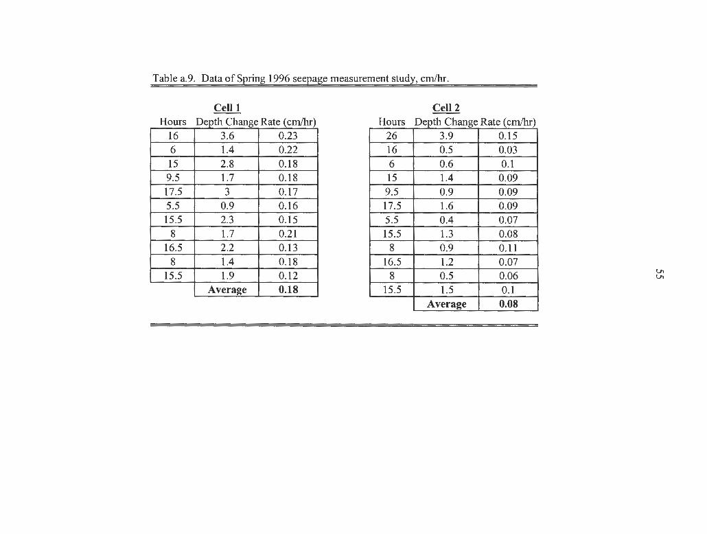
Table a.9. Data of Spring 1996 seepage measurement study, cm/hr.
Cell 1 Cell 2 Hours Depth Change Rate (cm/hr) Hours Depth Change Rate (cm/hr)
16 3.6 0.23 26 3.9 0.15 6 1.4 0.22 16 0.5 0.03 15 2.8 0.18 6 0.6 0.1 9.5 1.7 0.18 15 1.4 0.09 17.5 3 0.17 9.5 0.9 0.09 5.5 0.9 0.16 17.5 1.6 0.09 15.5 2.3 0.15 5.5 0.4 0.07
8 1.7 0.21 15.5 1.3 0.08 16.5 2.2 0.13 8 0.9 0.11
8 1.4 0.18 16.5 1.2 0.07 15.5 1.9 0.12 8 0.5 0.06
Average 0.18 15.5 1.5 0.1 Average 0.08
Vl Vl

Table a.9. Data of Spring 1996 seepage measurement study, cm/hr (continued).
Cell 3 Cell 4 Hours Depth Change Rate (cm/hr) - - Hours Depth Change Rate (cm/hr)
8 0.6 0.08 8 0.9 0.11 26 1.7 0.07 26 2.2 0.08 16 0.8 0.05 16 1.2 0.08 6 0.4 0.07 6 0.7 0.12 15 0.8 0.05 15 1.1 0.07 9.5 0.6 0.06 9.5 0.8 0.08 17.5 1 0.06 17.5 1.3 0.07 5.5 0.3 0.05 5.5 0.5 0.09 15.5 0.8 0.05 15.5 1.2 0.08
8 0.7 0.09 8 0.8 0.1 16.5 0.8 0.05 16.5 1.2 0.07
8 0.6 0.08 8 0.8 0.1 15.5 0.9 0.06 15.5 1 0.06
Average 0.06 Average 0.08
Vl O'I

Table a.9. Data of Spring 1996 seepage measurement study, cm/hr (continued).
Cell 5 Cell 6 Hours Depth Change Rate (cm/hr) Hours Depth Change Rate (cm/hr)
17 1.80 0.11 17 2.80 0.16 8 0.50 0.06 8 0.80 0.10
26 1.10 0.04 26 2.70 0.10 16 0.90 0.06 16 1.50 0.09 6 0.30 0.05 6 0.70 0.12 15 0.90 0.06 15 1.60 0.11 9.5 0.50 0.05 9.5 1.10 0.12 17.5 0.80 0.05 17.5 1.60 0.09 5.5 0.50 0.09 5.5 0.60 0.11 15.5 0.80 0.05 15.5 1.40 0.09
8 0.60 0.08 8 1.00 0.13 16.5 1.10 0.07 16.5 1.50 0.09
8 0.30 0.04 8 0.90 0.11 15.5 1.00 0.06 15.5 1.60 0.10
Average 0.06 Average 0.11
Vl -....)

Table a.9. Data of Spring 1996 seepage measurement study, cm/hr (continued).
Cell 7 Cell 8 Hours Depth Change Rate (cm/hr) Hours Depth Change Rate (cm/hr)
17 1.70 0.10 6 0.50 0.08 8 0.90 0.11 15 0.80 0.05
26 2.90 0.11 9.5 0.40 0.04 16 1.70 0.10 17.5 0.80 0.05 6 0.50 0.08 5.5 0.10 0.02 15 1.70 0.11 15.5 0.40 0.03 9.5 1.00 0.11 8 0.40 0.05 17.5 1.80 0.10 16.5 0.60 0.04 5.5 0.50 0.09 8 0.40 0.05 15.5 1.40 0.09 15.5 0.60 0.04
8 0.80 0.10 Average 0.05 16.5 1.50 0.09
8 0.70 0.09 15.5 1.60 0.10 Cell 9
Average 0.10 Hours Depth Change Rate (cm/hr) - -
17.5 1.60 0.09 8 1.00 0.13
16.5 3.00 0.18 8 1.40 0.18
15.5 2.10 0.14 I Average of all cells: 0.10 cm/hr I Average 0.05
Vl 00
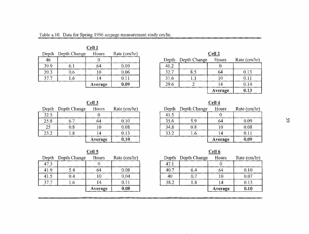
Table a.10. Data for Spring 1996 seepage measurement study cm/hr.
Cell 1 Depth Depth Change Hours Rate (cm/hr) Cell 2
46 0 Depth Depth Change Hours 39.9 6.1 64 0.10 41.2 0
39.3 0.6 10 0.06 32.7 8.5 64 37.7 1.6 14 0.11 31.6 1.1 10
Average 0.09 29.6 2 14 Average
Cell 3 Cell 4 Depth Depth Change Hours Rate (cm/hr) Depth Depth Change Hours 32.5 0 41.5 0 25 .8 6.7 64 0.10 35.6 5.9 64 25 0.8 10 0.08 34.8 0.8 10
23.2 1.8 14 0.13 33.2 1.6 14 Average 0.10 Average
Cell 5 Cell 6 Depth Depth Change Hours Rate (cm/hr) Depth Depth Change Hours 47.3 0 47.1 0 41.9 5.4 64 0.08 40.7 6.4 64 41.5 0.4 10 0.04 40 0.7 10 37.7 1.6 14 0.11 38.2 1.8 14
Average 0.08 Average
Rate (cm/hr)
0.13 0.11 0.14 0.13
Rate (cm/hr)
0.09 0.08 0.11 0.09
Rate (cm/hr)
0.10 0.07 0.13 0.10
Vl ID
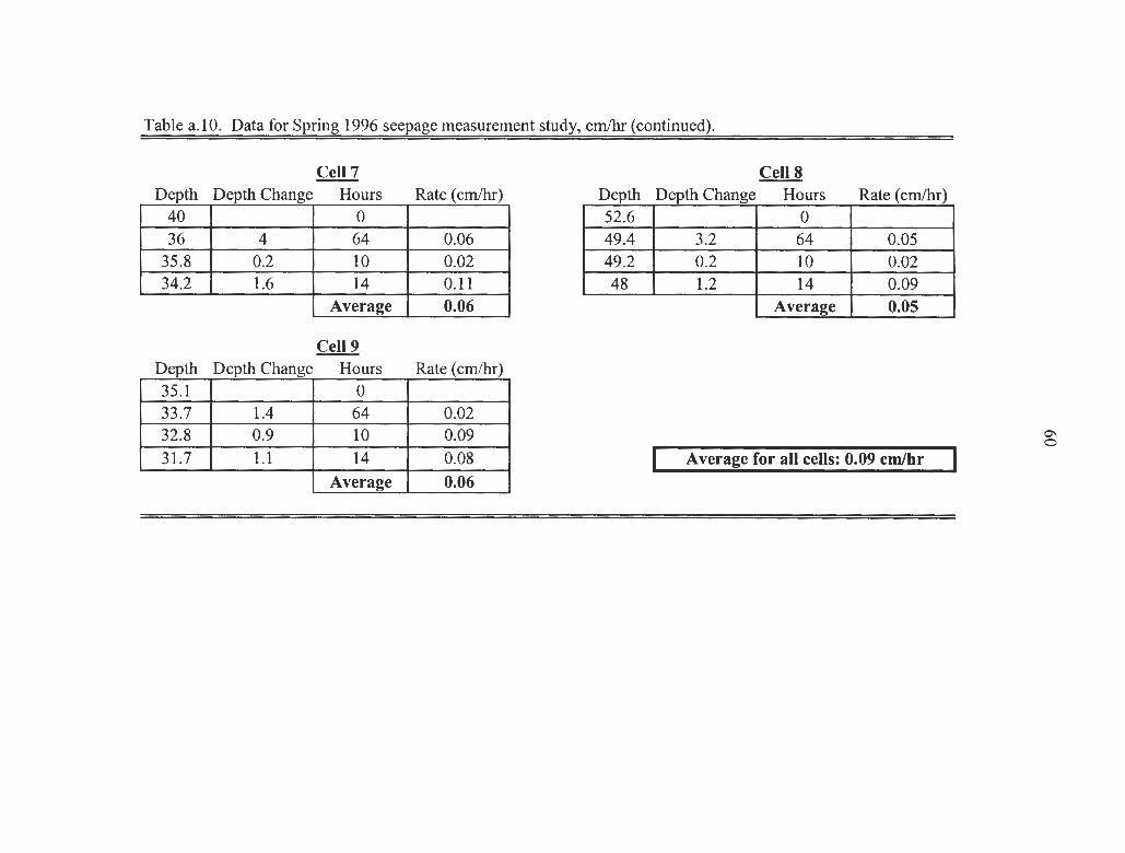
Table a. I 0. Data for Spring 1996 seepage measurement study, cm/hr (continued).
Cell 7 Cell 8 Depth Depth Change Hours Rate (cm/hr) Depth Depth Change Hours Rate (cm/hr)
40 0 52.6 0 36 4 64 0.06 49.4 3.2 64 0.05
35.8 0.2 10 0.02 49.2 0.2 10 0.02 34.2 1.6 14 0.11 48 1.2 14 0.09
Average 0.06 Average 0.05
Cell 9 Depth Depth Change Hours Rate (cm/hr) 35.1 0 33.7 1.4 64 0.02 32.8 0.9 10 0.09 31.7 1.1 14 0.08 I Average for all cells: 0.09 cm/hr I
Average 0.06
0\ 0

Table a.11. Data for Spring 1997 seepage measurement study, cm/hr.
Cell 1 Cell 2 Depth Depth Change Hours Rate (cm/hr) Depth Depth Change Hours Rate (cm/hr) 52.1 48.7 49.6 2.5 12.25 0.20 46.9 1.8 15.5 0.12 47.1 2.5 15.5 0.16 45 .6 1.3 9.75 0.13 45.5 1.6 9.75 0.16 44.4 1.2 10.25 0.12 43.7 1.8 10.25 0.18 43.2 1.2 7 0.17 42.6 1.1 7 0.16 41.1 2.1 18.5 0.11 39.8 2.8 18.5 0.15 39.8 1.3 9 0.14 38.4 1.4 9 0.16 38.5 1.3 14.5 0.09 36.6 1.8 14.5 0.12 37.6 0.9 9 0.10 35.5 1.1 9 0.12 36.1 1.5 14.25 0.11 33.7 1.8 14.25 0.13 35.4 0.7 5 0.14 0\
........
33.1 0.6 5 0.12 Average 0.12 Average 0.15
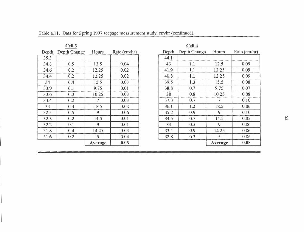
Table a.11. Data for Spring 1997 seepage measurement study, cm/hr (continued).
Cell 3 Cell 4 Depth Depth Change Hours Rate (cm/hr) Depth Depth Change Hours 35.3 44.1 34.8 0.5 12.5 0.04 43 1.1 12.5 34.6 0.2 12.25 0.02 41.9 1.1 12.25 34.4 0.2 12.25 0.02 40.8 1.1 12.25 34 0.4 15.5 0.03 39.5 1.3 15.5
33.9 0.1 9.75 0.01 38.8 0.7 9.75 33.6 0.3 10.25 0.03 38 0.8 10.25 33.4 0.2 7 0.03 37.3 0.7 7 33 0.4 18.5 0.02 36.1 1.2 18.5
32.5 0.5 9 0.06 35.2 0.9 9 32.3 0.2 14.5 0.01 34.5 0.7 14.5 32.2 0.1 9 0.01 34 0.5 9 31.8 0.4 14.25 0.03 33.1 0.9 14.25 31.6 0.2 5 0.04 32.8 0.3 5
Average 0.03 Average
Rate (cm/hr)
0.09 0.09 0.09 0.08 0.07 0.08 0.10 0.06 0.10 0.05 0.06 0.06 0.06 0.08
O'I N
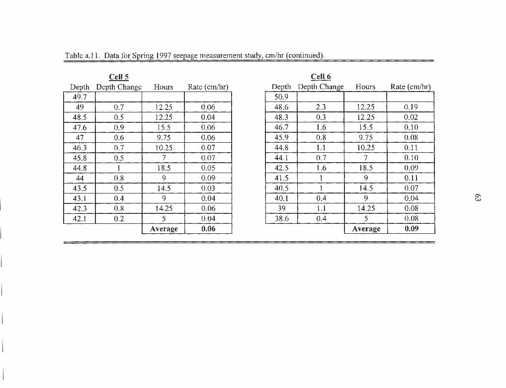
Table a.11. Data for Spring 1997 seepage measurement study, cm/hr (continued).
Cell 5 Cell 6 Depth Depth Change Hours Rate (cm/hr) Depth Depth Change Hours 49.7 50.9 49 0.7 12.25 0.06 48.6 2.3 12.25
48.5 0.5 12.25 0.04 48.3 0.3 12.25 47.6 0.9 15.5 0.06 46.7 1.6 15.5 47 0.6 9.75 0.06 45.9 0.8 9.75
46.3 0.7 10.25 0.07 44.8 1.1 10.25 45.8 0.5 7 0.07 44.1 0.7 7 44.8 1 18.5 0.05 42.5 1.6 18.5 44 0.8 9 0.09 41.5 1 9
43 .5 0.5 14.5 0.03 40.5 1 14.5 43 .1 0.4 9 0.04 40.1 0.4 9 42.3 0.8 14.25 0.06 39 1.1 14.25 42.l 0.2 5 0.04 38.6 0.4 5
Average 0.06 Average
Rate (cm/hr)
0.19 0.02 0.10 0.08 0.11 0.10 0.09 0.11 0.07 0.04 0.08 0.08 0.09
0\ w
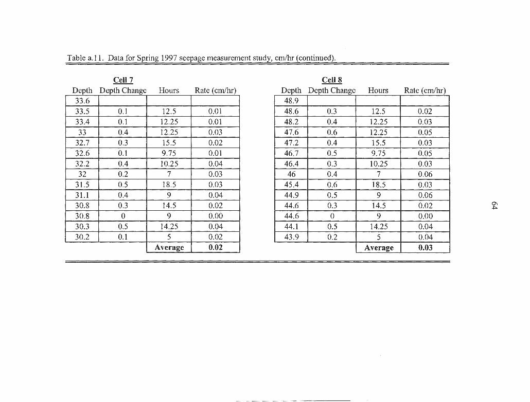
Table a.11. Data for Spring 1997 seepage measurement study, cm/hr (continued).
Cell 7 Cell 8 Depth Depth Change Hours Rate (cm/hr) Depth Depth Change Hours 33.6 48.9 33.5 0.1 12.5 0.01 48.6 0.3 12.5 33.4 0.1 12.25 0.01 48.2 0.4 12.25 33 0.4 12.25 0.03 47.6 0.6 12.25
32.7 0.3 15.5 0.02 47.2 0.4 15.5 32.6 0.1 9.75 0.01 46.7 0.5 9.75 32.2 0.4 10.25 0.04 46.4 0.3 10.25 32 0.2 7 0.03 46 0.4 7
31.5 0.5 18.5 0.03 45.4 0.6 18.5 31.1 0.4 9 0.04 44.9 0.5 9 30.8 0.3 14.5 0.02 44.6 0.3 14.5 30.8 0 9 0.00 44.6 0 9 30.3 0.5 14.25 0.04 44.1 0.5 14.25 30.2 0.1 5 0.02 43.9 0.2 5
Average 0.02 Average
Rate (cm/hr)
0.02 0.03 0.05 0.03 0.05 0.03 0.06 0.03 0.06 0.02 0.00 0.04 0.04 0.03
O'I ~
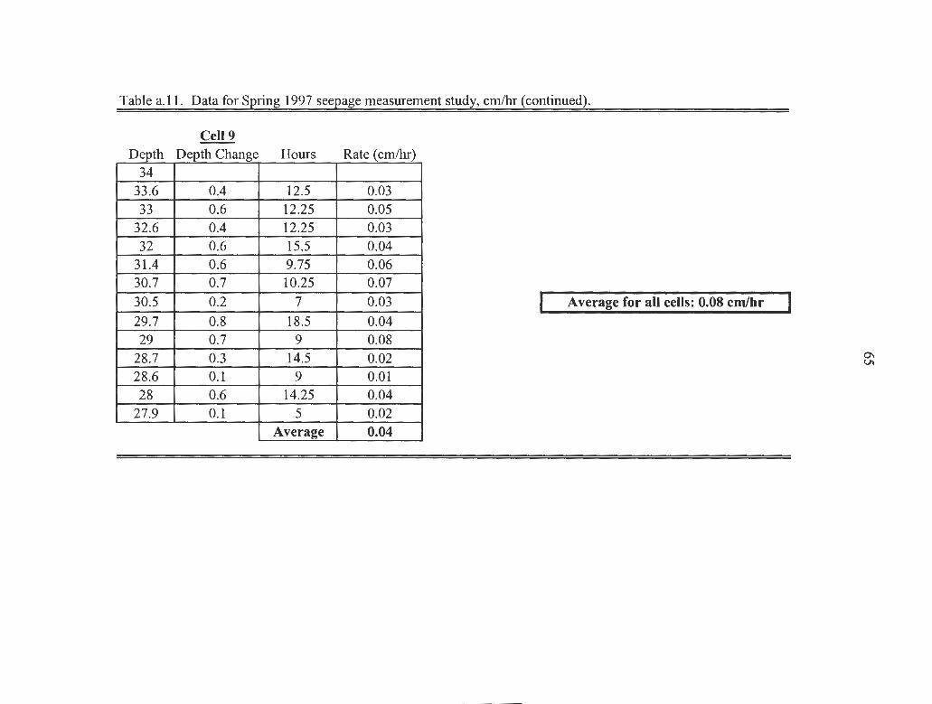
Table a.11. Data for Spring 1997 seepage measurement study, cm/hr (continued).
Cell 9 Depth Depth Change Hours - - -
Rate (cm/hr) 34
33.6 0.4 12.5 0.03 33 0.6 12.25 0.05
32.6 0.4 12.25 0.03 32 0.6 15.5 0.04
31.4 0.6 9.75 0.06 30.7 0.7 10.25 0.07 30.5 0.2 7 0.03 I Averagefor all cells: 0.08 cm/hr I 29.7 0.8 18.5 0.04 29 0.7 9 0.08
28.7 0.3 14.5 0.02 28.6 0.1 9 0.01 28 0.6 14.25 0.04
27.9 0.1 5 0.02 Average 0.04
0\ Vl

66
APPENDIXB
TRACER STUDY DATA
67
Table b.l. Wetland Cell 6 standards and fluorescence readings.
Hour 11 Hour 16.5 Standard Standard
Concentration Fluorescence Concentration Fluorescence (ppb) Reading (ppb) Readine
4.6 15 4.97 20 9.9 46 10.3 52
20.4 140 13.4 56 49.9 264 26.8 113 138.2 615 66.8 300 260.1 1155 102.3 450 426.4 1920 174.9 783
260.6 1182
Hour 34 Hour 61.5 Standard Standard
Concentration Fluorescence Concentration Fluorescence (ppb) Reading (ppb) Reading
2 74 2.74 83 5.96 155 5.58 163 12.66 294 11.54 304 27.2 680 24.89 625 59.4 1418 49.12 1212

Table b.2. Wetland Rh WT concentrations as derived from linear regression equations.
Sample Number
57 44 59 50 61 41 49 42 45 48 46 53 47 52 58 51 62 60 54 56
Hour 11 Fluorescence Concentration
Readin2 5 4
115 910 428 77 5
390 215 146 880
5 5 8
56 8 13
965 30
467
y = dye concentration, ppb x = fluorometer reading
(y = 0. 2223x) 1.11 0.89 25.56
202.29 95.14 17.12 1.11
86.70 47.79 32.46 195.62
1.11 1.11 1.78
12.45 1.78 2.89
214.52 6.67
103.81
Hour 16.5 Sample Fluorescence Number Readin2
86 487 85 339 65 456 64 632 72 6 75 496 79 100 70 310 73 89 81 53 77 48 80 92 71 13 66 234 69 680 74 440 76 263 84 397 68 347 82 160 63 227 78 316 67 297 83 23
Concentration (y = 0.2209x + 0.8932)
108.47 75.78 101.62 140.50 2.22
110.46 22.98 69.37 20.55 12.60 11.50 21.22 3.76 52.58 151.11 98.09 58.99 88.59 77.55 36.24 51.04 70.70 66.50 5.97
0\ 00

Table b.2. Wetland Rh WT concentrations as derived from linear regression equations (continued).
Sample Number
87 88 89 90 91 92 93 94 95 96 97 98 99 0 1 2 3 4 5 6 7 8 9 10
Hour 34 Fluorescence Concentration
Reading (y = 0.0422x - .6926) 1134 1235 750 1318 535 275 195 898 1522 1360 280 556 1436 590 597
2452 3083 1844 2311 1448 1868 1334 207
2268
y = dye concentration, ppb x = fluorometer reading
48.01 51.42 30.96 54.93 21.88 10.91 7.54
37.20 63.54 56.70 11.12 22.77 59.91 24.21 24.50 102.78 129.41 77.12 96.83 60.41 78.14 55.60 8.04
95.02
Hour 61.5 Sample Fluorescence Concentration Number Reading (y = 0.0413x - 0.9347)
71 644 25.66 75 582 23.10 66 288 10.96 72 445 17.44 64 671 26.78 74 530 20.95 73 1140 46.15 63 886 35.66 67 481 18.93 84 412 16.08 65 1187 48.09 61 790 31.69 78 373 14.47 79 700 27.98 68 643 25.62 70 635 25.29 76 918 36.98 81 543 21.49 77 646 25.75 80 234 8.73 62 515 20.33 63 990 39.95 69 759 30.41 82 785 31.49
O'\ \0

450
400
350
300
'""' .0 p.. p.. ';;' 250 0 ·.o o:s b i:: ~ 200 i:: 0 u
150
100
50
0
y = 0.2223x
R2 = 0.9986
--+- Standard
-Trendline
0 500 1000 1500 2000 2500
Fluorescence
Figure b.1. Standard curve and linear regression equation for rhodamine WT samples at hour 11.
-....) 0
,-.._ .D p. p. '-' i::: 0 -~
"' t: i::: II) u i::: 0 u
300
250
200
150 t 100
50
0 -
0 200 400
/
600 800
Fluorescence
y = 0.2209x + 0.8932 R2 = 0.9998
1000
-+- Standard
-Trendline
1200 1400
Figure b.2. Standard curve and linear regression equation for rhodamine WT samples at hour 16.5.
-....] ......

70
60
50
,-.._ .0 p.. 8 40 ~ 0
-~
~ g 30 0 u
20
10
--+-- Standard
-Trendline
0 +---~~~-1--~~~t--~~~1--~~--t~~~--t~~~-t-~~~-+~~~---1
0 200 400 600 800 1000 1200 1400 1600
Fluorescence
Figure b.3. Standard curve and linear regression equation for rhodamine WT samples at hour 34.
-.....} N

60
50
40 ~
.0 0..
i 30 + / -..] \.>.)
-+- Standard
-Trendline i:: 0 u i:: 0 u
20
10
O -+-~~~-----t-~~~~-+-~~~-----t-~~~~-+--~~~---t~~~~-t-~~~__,
0 200 400 600 800 1000 1200 1400
Fluorescence
Figure b.4. Standard curve and linear regression equation for rhodamine WT samples at hour 61.5.

74
APPENDIXC
RESIDENCE TIME DATA

75
Table c. l . 1996 Daily total flow rates and nominal residence time for each flow regime
High Flows Medium Flows Low Flows Flow Rate Residence Time Flow Rate Residence Time Flow Rate Residence Time
Date (ml/day) (days) (ml/day) (davs) (ml/day) (davs)
7/1 559 0.8 170 2.9 30 16.l 712 705 0.7 211 2.3 37 13. l 7/3 595 0.8 178 2.8 31 15.7 7/4 549 0.8 168 2.9 35 14.0 7/5 489 0.9 148 3.3 35 13.7 7/6 446 1.0 131 3.8 28 17.l 7/7 403 I.I 118 4.2 26 18.2 7/8 319 1.4 91 5.5 17 29.0 7/9 384 1.2 105 4.7 16 29.3 7/10 285 1.6 76 6.5 14 35.4 7/11 237 2.0 59 8.3 10 48.7 7/12 276 1.7 77 6.4 16 29.9 7/13 239 1.9 59 8.4 9 52.7 7/14 225 2.1 55 9.0 8 59.7 7/15 205 2.3 49 IO.I 7 70.5 7/16 185 2.5 42 11.7 5 94.9
7/19 928 0.5 401 1.2 122 3.9 7/20 883 0.5 254 1.9 73 6.6 7/21 679 0.7 215 2.3 60 8.0 7/22 556 0.8 170 2.9 43 I I.I 7/23 483 1.0 141 3.5 36 13.3 7/24 421 I.I 119 4.2 25 19.2 7/25 338 1.4 89 5.5 17 27.8 7126 292 1.6 75 6.6 14 33.8 7/27 251 1.8 64 7.7 14 34.6 7/28 302 1.5 98 5.0 43 11.3 7/29 256 1.8 66 7.5 15 31.5 7/30 245 1.9 60 8.3 13 37.8 7/31 197 2.3 45 11.0 7 65. l 8/1 184 2.5 41 12.0 6 87.l
814 148 3.1 26 19.3 3 145.8 815 485 1.0 164 3.0 60 8.1
8/8 262 1.8 67 7.3 14 33.8 8/9 216 2.1 51 9.7 8 57.3 8/10 188 2.5 37 13.5 6 84.5 8/ 11 196 2.4 46 10.9 12 38.9 8/12 161 2.9 33 14.9 8 59.8 8/13 142 3.2 27 18.3 7 69.9
8/16 97 4.8 13 36.7 I 719.5 8/17 95 4.9 14 34.7 I 389.5 8/18 86 5.4 10 51.8 0 1144.1
8/22 168 2.8 38 13.0 7 66.8 8/23 147 3.1 33 15.2 7 68.8 8/24 120 3.9 19 25.6 3 188.6 8/25 106 4.4 16 30.4 I 421.6
8/28 424 I.I 127 3.9 29 16.5 8129 326 1.4 89 5.5 20 24.3 8/30 261 1.8 66 7.5 14 33.9 8/31 214 2.2 51 9.7 10 46.9 911 180 2.6 41 12.l 8 60.9 9/2 149 3.1 32 15.5 6 86.4 9/3 127 3.7 22 22.2 4 137.4

76
Table c. l. 1996 Daily flow rates and nominal residence time for each flow regime, cont.
High Flow MediwnFlow Low Flow Flow Rate Residence Time Flow Rate Residence Time Flow Rate Residence Time
Date (m3/day) (davs) (m3/day) (davs) (m3/day) (da~ 914 108 4.3 17 29.0 3 167.3 915 97 4.8 13 37.7 2 308.0 916 79 5.8 9 52.4 I 471.3 917 76 6.1 9 56.l 0 1106.3 9/8 91 5.1 18 27.7 4 124.l 919 80 5.8 11 44.8 3 187.5 9/10 68 6.8 7 69.3 l 617.1 9/ 11 63 7.4 6 80.9 * * 9/12 57 8.1 5 92.5 * * 9/13 66 7.0 7 75.6 * * 9/14 43 10.7 4 113.2 * * 9115 43 10.7 4 120.5 * •
* • 9/18 34 13.8 3 150.5 • • 9/19 32 14.6 3 159.2 • * 9/20 46 IO.I 6 80.9 • • 9/21 31 14.7 2 235.3 • • 9/22 29 15.9 3 190.9 • • 9/23 39 12.0 6 88.2 • • 9/24 35 13.1 4 131.3 • • 9125 35 13.0 3 159.8 * *
9/28 572 0.8 163 3.0 54 8.9
10/2 295 1.6 73 6.8 19 24.9 10/3 253 1.8 57 8.7 19 26.0 10/4 258 1.8 61 8.1 15 32.l 10/5 245 1.9 56 8.9 14 33.4 10/6 230 2.0 51 9.7 17 28.9 1017 218 2.1 48 10.3 14 35.4 10/8 211 2.2 44 11.2 13 36.4 10/9 210 2.2 45 10.9 12 40.3
10/10 182 2.5 38 13.1 12 39.3 10/ 11 214 2.2 40 12.4 11 44.9 10/12 163 2.8 32 15.6 10 50.3 10/13 231 2.0 44 11.2 14 34.6 10/14 121 3.8 24 20.9 8 61.7 10115 159 2.9 32 15.5 8 61.2 10/16 154 3.0 27 18.1 8 57.9 10/17 167 2.8 34 14.7 10 49.5 10/18 141 3.3 27 18.4 8 64.1 10/19 138 3.4 22 22.7 6 84.5 10/20 140 3.3 25 20.2 6 83.5 10/21 125 3.7 22 22.0 9 53.5
10125 859 0.5 284 1.7 92 . 5.3 10126 696 0.7 221 2.2 53 9.1 10127 581 0.8 179 2.8 47 10.3
• Denotes no flow

77
Table c.2. 1997 Daily flow rates and nominal residence time for each flow regime.
High Flows Medium Flows Low Flows Flow Rate Residence Time Flow Rate Residence Time Flow Rate Residence Time
Date (m3/dav) (davs) (m3/dav) (davs) (m3/dav) (davs)
5/16 570 0.8 158 3.1 43 11.3 5/17 565 0.8 160 3.1 43 11.2 5/18 549 0.8 152 3.3 42 11.5 5/19 490 0.9 130 3.8 34 14.2 5120 452 1.0 120 4.1 33 14.7 5/21 442 1.0 116 4.3 35 13.6 5/22 435 1.1 113 4.4 28 17.2 5/23 426 1.1 111 4.5 30 16.0 5124 419 1.1 114 4.3 34 14.3 5125 418 1.1 112 4.4 32 15.0 5126 533 0.9 173 2.9 69 7.0 5/27 915 0.5 287 1.7 94 5.1 5/28 935 0.5 289 1.7 99 4.9 5129 976 0.5 305 1.6 105 4.6 5/30 970 0.5 298 1.7 99 4.9
615 531 0.9 142 3.5 40 12.2 6/6 581 0.8 163 3.0 47 10.2 617 521 0.9 143 3.5 41 11.8 6/8 553 0.8 148 3.3 41 11.8 619 394 1.2 101 4.9 28 17. l 6/10 409 1.1 105 4.7 28 17.3 6/11 412 1.1 104 4.7 30 16.2 6/12 424 1.1 128 3.9 44 10.9 6/13 409 1.1 107 4.6 31 15.6 6/14 383 1.2 96 5.2 27 18.0 6115 372 1.2 102 4.8 25 19.3 6/16 368 1.3 78 6.4 25 19.3 6/17 334 1.4 88 5.6 18 26.2 6/18 362 1.3 106 4.7 35 13.8 6119 360 1.3 91 5.5 16 29.7 6/20 340 1.4 85 5.8 23 21.1
6125 763 0.6 324 1.5 103 4.7 6/26 621 0.7 279 1.8 82 5.9 6/27 740 0.6 229 2.2 66 7.3 6/28 661 0.7 184 2.7 67 7.2 6/29 542 0.9 154 3.2 31 15.5 6/30 512 0.9 152 3.3 47 10.3 711 472 1.0 128 3.8 38 12.9 7/2 401 1.2 102 4.9 29 16.9 7/3 350 1.3 80 6.1 23 21.4 7/4 338 1.4 79 6.3 23 21.2 715 312 1.5 69 7.2 20 23.7 716 289 1.6 61 8.1 17 28.0 717 266 1.7 51 9.6 16 30.2 7/8 257 1.8 48 10.3 16 30.2 719 229 2.0 39 12.6 12 40.2 7/10 217 2.1 34 14.5 12 41.4 7/11 227 2.0 37 13.5 4 112.9 7/12 217 2.1 35 14.2 2 272.6 7/13 201 2.3 30 16.7 I 360.6 7/14 191 2.4 25 19.5 1 463.0 7/15 171 2.7 16 30.4 * * 7/16 163 2.8 11 44.5 * * 7/17 145 3.2 16 31.7 * *
7/19 123 3.8 * * * *
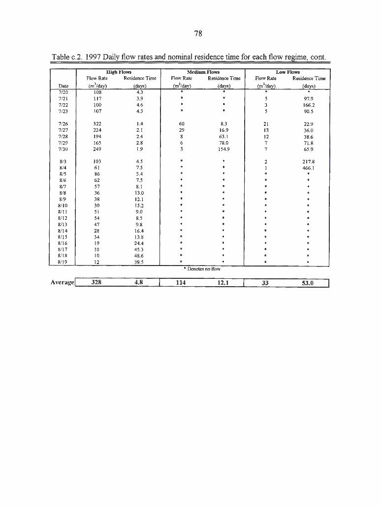
78
Table c.2. 1997 Daily flow rates and nominal residence time for each flow regime, cont.
High Flows Medium Flows Low Flows Flow Rate Residence Time Flow Rate Residence Time Flow Rate Residence Time
Date (m3/day) (days) (m3/day) (days) (m3/day) (days)
7/20 108 4.3 • • • • 7/21 117 3.9 • • 5 97.9 7/22 100 4.6 • • 3 166.2 7/23 107 4.3 • • 5 90.5
7/26 322 1.4 60 8.3 21 22.9 7/27 224 2.1 29 16.9 13 36.0 7/28 194 2.4 8 63. l 12 38.6 7/29 165 2.8 6 78.0 7 71.8 7/30 249 1.9 3 154.9 7 65.9
8/3 103 4.5 • • 2 217.8 8/4 61 7.5 • • 1 466.l 815 86 5.4 • • • • 8/6 62 7.5 • • • • 817 57 8.1 • • • • 8/8 36 13.0 • • • • 8/9 38 12.1 • • • • 8/10 30 15.2 • • • • 8/11 51 9.0 • • • • 8/12 54 8.5 • • • • 8/ 13 47 9.8 • • • • 8/14 28 16.4 • • • • 8/ 15 34 13.8 • • • • 8/16 19 24.4 • • • • 8/17 10 45.3 • • • • 8/18 10 48.6 • • • • 8/19 12 39.5 • • • •
• Denotes no flow
Average~'~~32_8~~~~-4-.8~~.._~_11_4~~~~1_2_.1~--''--~-3_3~~~__;5~3~.0;..._--1

,..... ;>, ~ -= -..... e .._, ~
~ it: = r;;
1000
900
800
700
600
500
400
300
200
100
1 .. .. , . . ~ # • .. . ..
a ,• . ~ ,
---Total Flow Rate
- - - - - -Residence Time
' . : .
:
I ' ... .. ~
. : . " . ... .. . . . . . . . . . . . . . . .. . .. . .. . ..
' .. . . -. . .
. .. ... .. . ' .
. .... -.. . ~·
18
16
14
12
";;'
~ -= 10 .._, e E= ~ ~
8 5 :s "' ~
6
4
2
0 0
August September October
1996
Figure c.1. Comparison of flow rates and nominal residence times for high flow cells totals during the 1996 season.
-.) \0

450
400 ---Total Flow Rate
- - - - - -Residence Time
350
300
.. .
. It I J
250
200
tl1 I,. ~
~ : : : : ;: 150 ~ ~ I I I I 11 "'O
"C 250 . " . " '-' ,.,,.......... I 11 I 1 1 Q.} a .... ,. e ~ : :: :; : E= ~ I :· :I: ~ =: 200 A . .: . ; . = 000 :. I I I I Q,.)
~ I .: •: I :s - . ' ·. . 100 I#>
~ : " :. : ~ .: ; : ! I
150 + \ I \ I : :; ' I
100 50
50
.. . ....... •' • L•I ---· . -·· • ~ 0 0 1----- --·
. •'
August September October
1996
Figure c.2. Comparison of flow rates and nominal residence times for medium flow cell totals during the 1996 season.
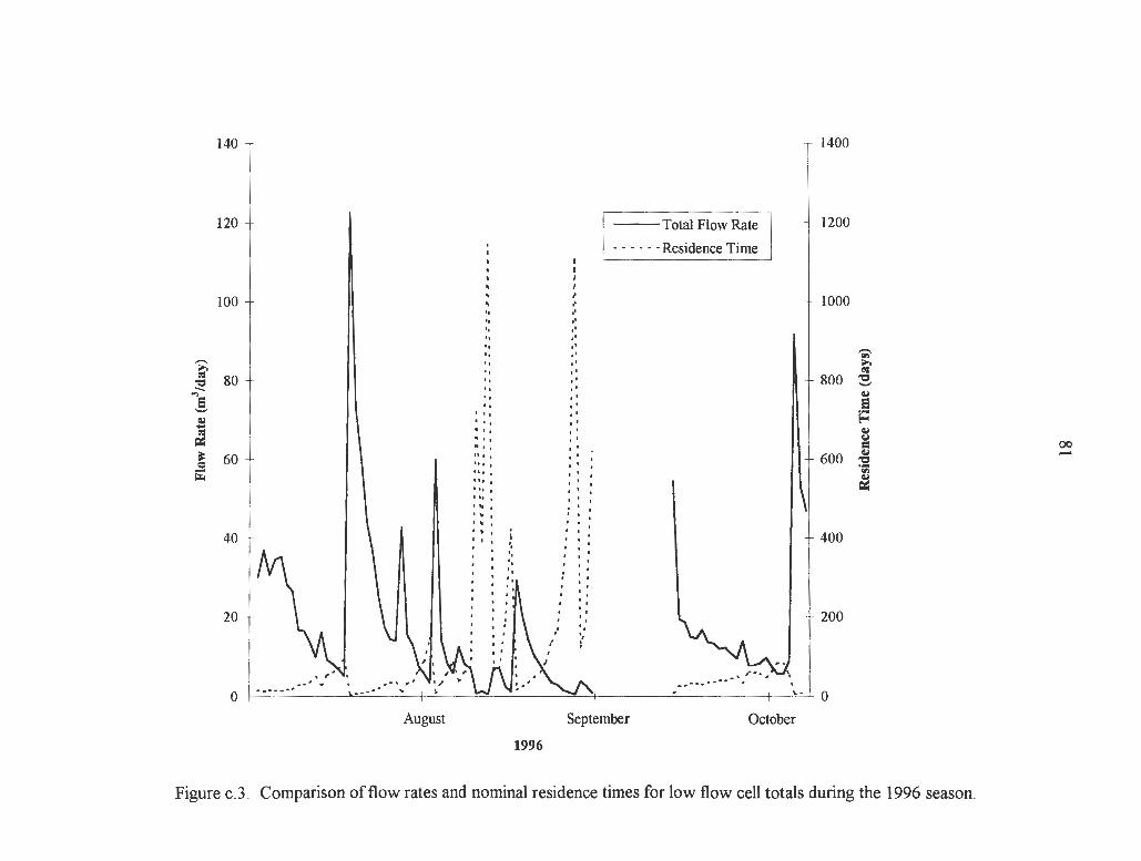
140 1400
120 + I I Total Flow Rate I + 1200
- - - -Residence Time
100 t II . Loo • I
'• •' '• •' '• •' '• •' '• •' '• ,. '";;'
,-.. .. •' ~ ~ .. , . C<:l 80 '• " 800 -= -= .._, .._ .. " QJ .., .. " e '• •' e .._, ... •' !=: QJ .. , .. ~ . '' .. QJ ... . . y ... . . = 00
~ 60 U1 I . ' . 600 QJ -I -= "1 I . ' . . ..
l\1 I ... "' ~ 111 I ... I ~ 111 I .. 111 I
'~ . . ' .. .. ' . '
40 t A - I \ ~ II . '. I . I I + 400 o I' . .. . ' •,
'• •,
. :~ . . . l I l 200
. . . . ' 20+ \ I \ II II . . . . . .
.... ,. -.... -...... 0
...... -...... ...... .. .. " ~- 0
August September October
1996
Figure c.3. Comparison of flow rates and nominal residence times for low flow cell totals during the 1996 season.
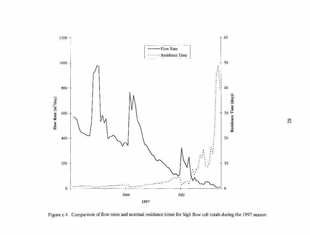
-.... co: "Cl --.., e .._, ~ ... ~
£
1200
1000
800
600
400
200
---Flow Rate
· · · · · · Residence Time
,, .. # '
' f
. . . . ... ... I •'
,. ,1 '. I¥ I I ..
:
60
50 . . . . . ' . ' . . . . . . . . 40
30
20
I
10
___ ............ .. 0 .... ··········-·------- - 0 ....................
June July
1997
-"' .... co:
"Cl .._, ~ e ~ ~ lo.I = ~
"Cl ·;;
~
Figure c.4. Comparison of flow rates and nominal residence times for high flow cell totals during the 1997 season.
00 N
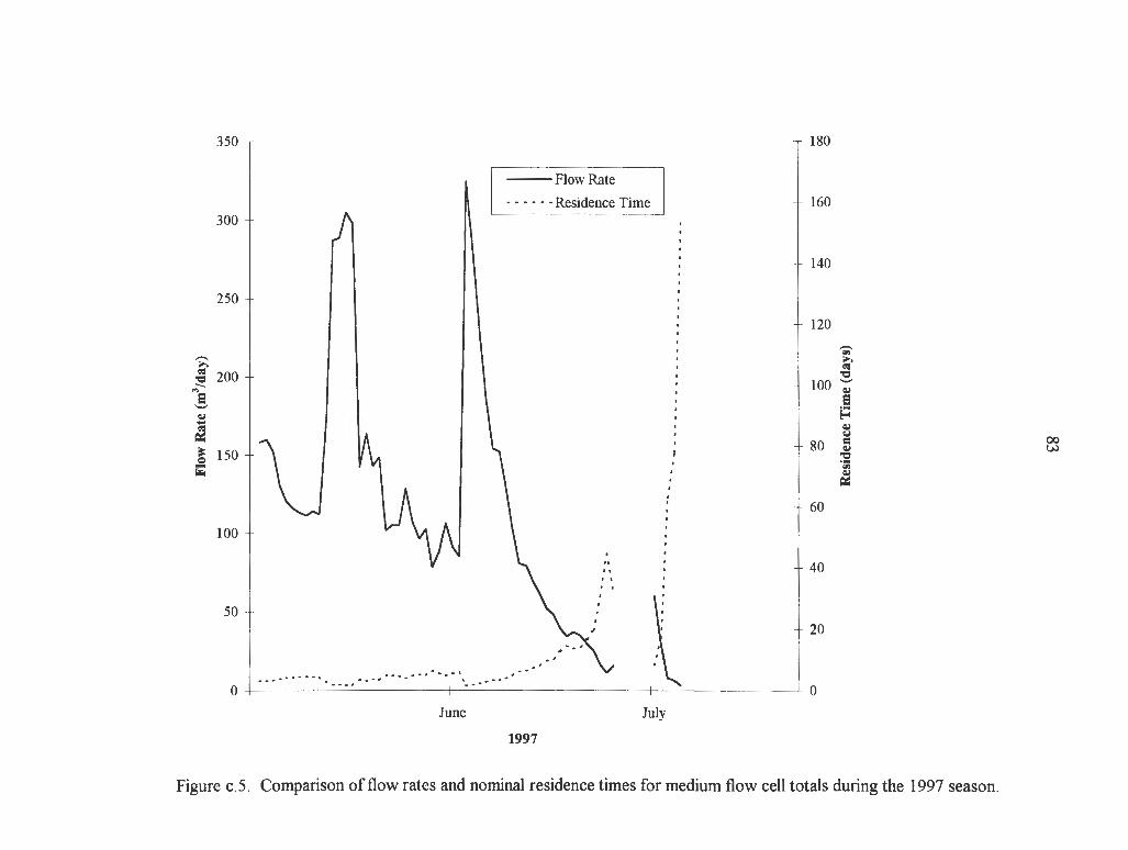
350 T T 180
Flow Rate
- - - - - -Residence Time I + 160 300
' ' ' ' 140 ' '
250 ' '
120
-;;-,-... ..... ' ..... ~ 200 ' elS
' 'Cl
-- ' 100 ';;' "' ' El .._, ' El ~
' ~ ' ~ ' ~
~ ' (j
\ ' 80 = 00 ~ 150 I ~ w Q
' :'5!
fi: "" ' ~ 60
100
40
50 20
0 - - - - - - - - - .• - - - • - - - . - - . - - . - • - - .. _ - - - - - - ~ 0
June July
1997
Figure c. 5. Comparison of flow rates and nominal residence times for medium flow cell totals during the 1997 season.
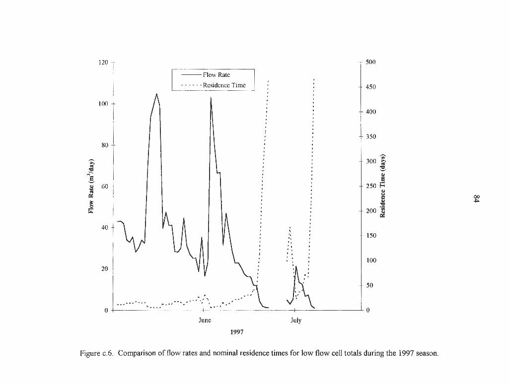
120 500
---Flow Rate
- - - - - -Residence Time 450
100 400
350 80
-~ -..... ~
"Cl
300 i;' "Cl .._, --..,
E! .._, ~ 60 ~ = j i;;i..
~
E! 250 E=
~ y
= 00 ~ .;:...
"Cl 200 ·;;
~ 40
I \ I I II I II I '• '•
150 '• '' '' '' '
I \I I J ~ ' ' 100 20
50
0 ... ~--·""· .--··,: ... •••I # I
0
June July
1997
Figure c.6. Comparison of flow rates and nominal residence times for low flow cell totals during the 1997 season.
85
REFERENCES CITED
Adamkus, V.W. 1976. The future ofnonpoint pollution control: A federal perspective. In: Procedures of the conference on nonpoint sources of water pollution problems, policies, and prospects. Purdue University, West Lafayette, Indiana.
Bowmer, K.H. 1987. Nutrient removal from effluents by an artificial wetland: Influence of rhizosphere aeration and preferential flow studied using bromide and dye tracers. Water Research, 21 :591-599.
Carey, A.E. 1991. Agriculture, agricultural chemicals, and water quality. pp. 78-85. In: Agriculture and the environment: The 1991 yearbook of agriculture. U.S. Government Printing Office, Washington, D.C ..
Cooper, AB. 1994. Coupling wetland treatment to land treatment: An innovative method for nitrogen stripping? Water Science Technology, 29 (4):141-149.
Crumpton, W.G., T.M. Isenhart, and S.W. Fisher. 1993 . Fate of non-point source nitrate loads in freshwater wetlands: Results from experimental wetland mesocosms. pp. 283-291. In: Constructed wetlands for water quality improvement. G.A. Moshiri (Ed.). Lewis Publishers. Chelsea, Michigan.
Dahl, T.E. 1990. Wetlands losses in the United States, 1780's to 1980's. U.S . Department of the Interior, Fish and Wildlife Service. Washington, D.C.
Feuerstein, D.W. and R.E. Selleck. 1963 . Fluorescent tracer for dispersion measurements. Proceedings of the American Society of Civil Engineering Journal of Sanitary Engineering Division. 89(SA4): 1-21.
Hammer, D.A., (editor) 1989. Constructedwetlandsforwastewater treatment. Municipal, industrial and agricultural. Lewis Publishers. Chelsea, Michigan.
Hammer, D.A. and R.K. Bastian. 1989. pp. 5-19. Wetlands ecosystems: natural water purifiers? In: Constructed wetlands for wastewater treatment. Municipal, industrial and agricultural. D.A. Hammer (Ed.). Lewis Publishers. Chelsea, Michigan.
Hammer, D.A. and R.L. Knight. 1994. Designing constructed wetlands for nitrogen removal. Water Science Technology, 29(4) :15-27.
Hershkowitz, J. 1986 Listowel Artificial Marsh Project Report. Ontario Ministry of the Environment, Water Resources Branch. Toronto. 251 pp.

86
Hey, D.L., K. Barrett, and C. Biegen. 1992. The Hydrology of Four Experimental Wetlands. Volume 2, Chapter 1. In: The Des Plaines River Wetlands Demonstration Project. Wetlands Research, Inc. Chicago, Illinois.
Hey, D.L., AL. Kenimer, and K.R. Barrett. 1994. Water quality improvement by four experimental wetlands. Ecological Engineering. 3(4):381-398.
Higgins, M.J., C.A. Rock, R. Bouchard, and B. Wengrezynek. 1993. Controlling agricultural runoff by use of constructed wetlands. In: Constructed Wetlands for water quality improvement. G.A. Moshiri (Ed.). Lewis Publishers. Boca Raton, Florida.
Kadlec, R.H. 1993. Hydrologic factors in wetland water treatment. pp. 21-40. In: Constructed wetlands for wastewater treatment. D.A. Hammer (Ed.). Lewis Publishers. Chelsea, Michigan.
Kadlec, R.H., W. Bastiaens, and D.T. Urban. 1993. Hydrological design of free water surface treatment wetlands. pp. 77-86. In: Constructed wetlands for water quality improvement. G.A. Moshiri (Ed.). Lewis Publishers. Boca Raton, Florida.
Kadlec. R.H. 1994. Detention and mixing in free water wetlands. Ecological Engineering, 3:345-380.
Kadlec, R.H. and R.L. Knight. 1996. Treatment wetlands. CRC Lewis Publishers. Boca Raton, Florida.
Knight, R.L. 1994. Treatment wetlands database now available. Water Environment Technology, 6 (2):31-33 .
Midwest Plan Service. 1993. Livestock Waste Facilities Handbook. Midwest Plan Service, Iowa State University, Ames, Iowa. 6.1.
Mitsch, W.J. and J.G. Gosselink. 1993. Wetlands. Van Nostrand Reinhold Company. New York.
Moshiri, G.A., (editor) 1994. Constructed wetlands for water quality improvement. Lewis Publishers. Boca Raton, Florida.
Novotny, V. and G. Chesters. 1981. Handbook ofnonpoint pollution sources and management. Van Nostrand Reinhold Company. New York.
Reed, S. C. 1991. Constructed wetlands for wastewater treatment. Biocycle, 3 2 ( 1) :44.
Smart, P.L. and I.M.S. Laidlaw. 1977. An evaluation of some fluorescent dyes for water tracing. Water Resources Research, 13 (1):15-33 .

87
TVA (Tennessee Valley Authority). 1990. Unpublished dye study results from September 1990 at Benton, Kentucky.
van der Valk, A.G. and R.W. Jolly. 1992. Recommendations for research to develop guidelines for the use of wetlands to control rural NPS pollution. Ecological Engineering, 1: 115-134.
Wetlands Research, Inc. (WRI). 1992. The Des Plaines River Wetlands Demonstration Project. Report to USEPA, July 1992, 7 Volumes, Wetlands Research, Inc. Chicago, Illinois.