Hydrologic Simulations of the Maquoketa River Watershed Using SWAT

Manoj Jha

Working Paper 09-WP 492 June 2009

Center for Agricultural and Rural Development Iowa State University

Ames, Iowa 50011-1070 www.card.iastate.edu

Manoj Jha is an associate scientist in the Center for Agricultural and Rural Development at Iowa State University. This paper is available online on the CARD Web site: www.card.iastate.edu. Permission is granted to excerpt or quote this information with appropriate attribution to the authors. Questions or comments about the contents of this paper should be directed to Manoj Jha, 560E Heady Hall, Iowa State University, Ames, Iowa 50011-1070; Ph: (515) 294-7695; Fax: (515) 294-6336; E-mail: manoj@iastate.edu. Iowa State University does not discriminate on the basis of race, color, age, religion, national origin, sexual orientation, gender identity, sex, marital status, disability, or status as a U.S. veteran. Inquiries can be directed to the Director of Equal Opportunity and Diversity, 3680 Beardshear Hall, (515) 294-7612.

Abstract

 

This paper describes the application of the Soil and Water Assessment Tool (SWAT)

model to the Maquoketa River watershed, located in northeast Iowa. The inputs to the model

were obtained from the Environmental Protection Agency’s geographic information/database

system called Better Assessment Science Integrating Point and Nonpoint Sources (BASINS).

Climatic data from six weather stations located in and around the watershed, and measured

streamflow data from a U.S. Geological Survey gage station at the watershed outlet were

used in the sensitivity analysis of SWAT model parameters as well as its calibration and

validation for watershed hydrology and streamflow. A sensitivity analysis was performed

using an influence coefficient method to evaluate surface runoff and baseflow variations in

response to changes in model input hydrologic parameters. The curve number, evaporation

compensation factor, and soil available water capacity were found to be the most sensitive

parameters among eight selected parameters when applying SWAT to the Maquoketa River

watershed. Model calibration, facilitated by the sensitivity analysis, was performed for the

period 1988 through 1993, and validation was performed for 1982 through 1987. The model

performance was evaluated by well-established statistical methods and was found to explain

at least 86% and 69% of the variability in the measured streamflow data for the calibration

and validation periods, respectively. This initial hydrologic modeling analysis will facilitate

future applications of SWAT to the Maquoketa River watershed for various watershed

analyses, including water quality.

Keywords: calibration and validation, hydrologic simulation, sensitivity analysis, SWAT.

1

1. Introduction

Hydrology is the main governing backbone of all kinds of water movement and hence of

water-related pollutants. Understanding the hydrology of a watershed and modeling different

hydrological processes within a watershed are therefore very important for assessing the

environmental and economical well-being of the watershed. Simulation models of watershed

hydrology and water quality are extensively used for water resources planning and

management. These models can offer a sound scientific framework for watershed analyses of

water movement and provide reliable information on the behavior of the system. New

developments in modeling systems have increasingly relied on geographic information

systems (GIS) that have made feasible large area simulation, and on database management

systems such as Microsoft Access to support modeling and analysis.

Several watershed-scale hydrologic and water quality models such as HSPF

(Hydrological Simulation Program - FORTRAN) (Johansen et al., 1984), HEC-HMS

(Hydrologic Modeling System) (USACE-HEC, 2002), CREAMS (Chemical, Runoff, and

Erosion from Agricultural Management Systems) (Knisel, 1980), EPIC (Erosion-Productivity

Impact Calculator) (Williams et al., 1984), AGNPS (Agricultural Non-Point Source) (Young

et al., 1989), and SWRRB (Simulator for Water Resources in Rural Basins) (Arnold et al.,

1990) have been developed for watershed analyses. While these models are very useful, they

are generally limited in several aspects of watershed modeling, such as inappropriate scale,

inability to perform continuous-time simulations, inadequate maximum number of

subwatersheds, and the inability to characterize the watershed in enough spatial detail (Saleh

et al., 2000). A relatively recent model developed by the U.S. Department of Agriculture

(USDA) called SWAT (Soil and Water Assessment Tool) (Arnold et al., 1998) has proven

2

very successful in the watershed assessment of hydrology and water quality. It has been used

extensively worldwide (Gassman et al., 2007) as evidenced by over 500 peer-reviewed

publications on the model (personal communication, Jeffery G. Arnold, USDA-ARS,

Temple, Texas). SWAT is a physically based model and offers continuous-time simulation, a

high level of spatial detail, an unlimited number of watershed subdivisions, efficient

computation, and the capability of simulating changes in land management. An early

application of the model by Arnold and Allen (1996) compared the results of SWAT to

historical streamflow and groundwater flow in three Illinois watersheds. Arnold and Allen

found that the model was able to simulate all the components of the hydrologic budget within

acceptable limits on both annual and monthly time steps. The Natural Resources

Conservation Service (NRCS) used the SWAT model in the 1997 Resource Conservation

Appraisal. The model was validated against measured streamflow and sediment loads across

the entire U.S. (Arnold et al., 1999). The effect of spatial aggregation on SWAT was

examined by FitzHugh and Mackay (2000) and Jha et al. (2004a). SWAT applications for

flow and/or pollutant loadings have compared favorably with measured data for a variety of

watershed scales (Srinivasan et al., 1998; Arnold et al., 1999; Saleh et al., 2000; Santhi et al.,

2001). The SWAT model was successfully applied to assess the impact of climate change in

hydrology of the Upper Mississippi River Basin (Jha et al., 2004b) and the Missouri River

Basin (Stone et al., 2001). SWAT has been chosen by the Environmental Protection Agency

to be one of the models of their Better Assessment Science Integrating Point and Nonpoint

Sources (BASINS) (Whittemore, 1998).

Besides successful application of physically based models, there are several issues that

question the model output such as uncertainty in input parameters, nonlinear relationships

3

between hydrologic input features and hydrologic response, and the required calibration of

numerous model parameters. These issues can be examined with sensitivity analyses of the

model parameters to identify sensitive parameters with respect to their impacts on model

outputs. Proper attention to the sensitive parameters may lead to a better understanding and

to better estimated values and thus to reduced uncertainty (Lenhart et al., 2002). Knowledge

of sensitive input parameters is beneficial for model development and leads to a model’s

successful application. Arnold et al. (2000) performed a sensitivity analysis of three

hydrologic input parameters of the SWAT model against surface runoff, baseflow, recharge,

and soil evapotranspiration on three different basins within the Upper Mississippi River

Basin. Spruill et al. (2000) selected fifteen hydrologic input variables of the SWAT model

and varied them individually within acceptable ranges to determine model sensitivity in daily

streamflow simulation. They found that the determination of accurate parameter values is

vital for producing simulated streamflow data in close agreement with measured streamflow

data. Two simple approaches of sensitivity analysis were compared by Lenhart et al. (2002)

using the SWAT model on an artificial catchment. In both approaches, one parameter was

varied at a time while holding the others fixed except that the way of defining the range of

variation was different: the first approach varied the parameters by a fixed percentage of the

initial value and the second approach varied the parameters by a fixed percentage of the valid

parameter range. Lenhart et al. found similar results for both approaches and suggested that

the parameter sensitivity may be determined without the results being influenced by the

chosen method. The paper identified several most sensitive hydrologic and plant-specific

parameters but emphasized that sensitivities can be different for a natural catchment because

of oversimplification of the processes in the chosen artificial catchment.

4

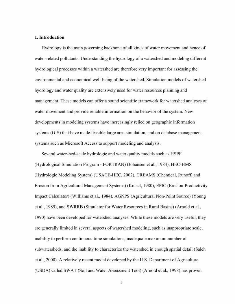
In this study, SWAT was applied to the Maquoketa River watershed (MRW), located in

northeast Iowa (Figure 1). The objectives of this study were to identify the SWAT’s

hydrologic sensitive parameters relative to the estimation of surface runoff and baseflow, and

to calibrate and validate the model for streamflow. The influence coefficient method was

used to examine surface runoff and baseflow responses to changes in model input

parameters. The parameters were ranked according to the magnitudes of response variable

sensitivity to each of the model parameters, which divide high and low sensitivities. The

SWAT model was calibrated by varying the values of sensitive parameters (as identified in

the sensitivity analysis) within their permissible values and then compared simulated

streamflow with the measured streamflow at the watershed outlet. This study will facilitate

future applications of the SWAT model to the MRW, which will support efforts to mitigate

water quality problems in the region.

2. Materials and methods

2.1 The SWAT model

The SWAT model is a long-term, continuous simulation watershed model. It operates on a

daily time step and is designed to predict the impact of management on water, sediment, and

agricultural chemical yields. The model is physically based, computationally efficient, and

capable of simulating a high level of spatial detail by allowing the division of watersheds into

smaller subwatersheds. SWAT models water flow, sediment transport, crop/vegetation

growth, and nutrient cycling. The model allows users to model watersheds with less

monitoring data and to assess predictive scenarios using alternative input data such as

climate, land-use practices, and land cover on water movement, nutrient cycling, water

5

quality, and other outputs. Major model components include weather, hydrology, soil

temperature, plant growth, nutrients, pesticides, and land management. Several model

components have been previously validated for a variety of watersheds.

In SWAT, a watershed is divided into multiple subwatersheds, which are then further

subdivided into Hydrologic Response Units (HRUs) that consist of homogeneous land use,

management, and soil characteristics. The HRUs represent percentages of the subwatershed

area and are not identified spatially within a SWAT simulation. The water balance of each

HRU in the watershed is represented by four storage volumes: snow, soil profile (0-2

meters), shallow aquifer (typically 2-20 meters), and deep aquifer (more than 20 meters). The

soil profile can be subdivided into multiple layers. Soil water processes include infiltration,

evaporation, plant uptake, lateral flow, and percolation to lower layers. Flow, sediment,

nutrient, and pesticide loadings from each HRU in a subwatershed are summed, and the

resulting loads are routed through channels, ponds, and/or reservoirs to the watershed outlet.

Detailed descriptions of the model and model components can be found in Arnold et al.

(1998) and Neitsch et al. (2002).

2.2 Maquoketa River watershed and SWAT input data

The Maquoketa River watershed (MRW) covers 4,867 km2 of predominantly agricultural

land in northeast Iowa (Figure 1). The MRW is one of 13 tributaries of the Mississippi River

that have been identified as contributing some of the highest levels of suspended sediments,

nitrogen, and phosphorus to the Mississippi stream system

(http://www.umesc.usgs.gov/data_library/sediment_nutrients/sediment_nutrient_page.html).

These pollution loads are attributed mainly to agricultural nonpoint sources and result in

6

degraded water quality within each watershed, in the Mississippi River, and ultimately in the

Gulf of Mexico.

Land use, soil, and topography data required for simulating the watershed were obtained

from the BASINS package version 3 (USEPA, 2001). Topographic information is provided

in BASINS in the form of Digital Elevation Model (DEM) data. The DEM data were used to

generate variations in subwatershed configurations such as subwatershed delineation, stream

network delineation, and slope and slope lengths using the ArcView interface for the SWAT

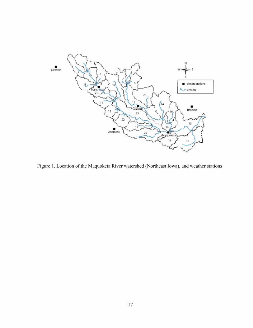
2000 model (AVSWAT) (Di Luzio et al., 2000). Land-use categories provided in BASINS

are relatively simplistic, including only one category for agricultural land (defined as

“Agricultural Land-Generic” or AGRL). Agricultural lands cover almost 90% of the MRW;

the remaining area is mostly forest (Figure 2). The soil data available in BASINS comes from

the State Soil Geographic (STATSGO) database (USDA, 1994), which contains soil maps at

a 1:250,000 scale. Each STATSGO map unit is linked to the Soil Interpretations Record

attribute database that provides the proportionate extent of the component soils and soil layer

properties. The STATSGO soil map units and associated layer data were used to characterize

the simulated soils for the SWAT analyses.

The daily climate inputs consist of precipitation, maximum and minimum temperatures,

solar radiation, wind speed, and relative humidity. In case of missing observed data or the

absence of complete data, the weather generator within SWAT uses its statistical database to

generate representative daily values for the missing variables for each subwatershed.

Historical daily precipitation and daily maximum and minimum temperatures were obtained

from the Iowa weather database (www.mesonet.agron.iastate.edu) for the six climate stations

located in or near the watershed (see Figure 1). The management operations required for the

7

HRUs were defaulted by AVSWAT and consisted simply of planting, harvesting, and

automatic fertilizer applications for the agricultural HRUs.

2.3 Sensitivity Analysis

The influence coefficient method is one of the most common methods for computing

sensitivity coefficients in surface and ground water problems (Helsel and Hirsch, 1992). The

method evaluates the sensitivity by changing each of the independent variables, one at a time.

A sensitivity coefficient represents the change of a response variable that is caused by a unit

change of an explanatory variable, while holding the rest of the parameters constant:

( ) ( )i

NiNii

PPPPPFPPPPPF

PF

Δ−Δ+

=ΔΔ ,....,...,,,....,...,, 2121 (1)

where F is the response variable, P is the independent parameter, and N is the number of

parameters considered. The sensitivity coefficients can be positive or negative. A negative

coefficient indicates an inversely proportional relation between a response variable and an

explanatory parameter.

To meaningfully compare different sensitivities, the sensitivity coefficient was normalized

by reference values, which represent the ranges of each pair of dependent variable and

independent parameter. The normalized sensitivity coefficient is called the sensitivity index

and is given as (Gu and Li, 2002):

8

PF

FP

sm

mi Δ

Δ= (2)

where si is the sensitivity index, and Fm and Pm are the mean of lowest and highest values of

the selected range for the explanatory parameter and the response variable, respectively. A

higher absolute value of sensitivity index indicates higher sensitivity and a negative sign

shows inverse proportionality.

2.4 Simulation Approach

The AVSWAT model (ArcView interface of the SWAT model) was used in the

watershed delineation process, which includes processing of DEM data for stream network

delineation followed by subwatershed delineation. A total of 25 subwatersheds were

delineated for the entire MRW (see Figure 1). The subwatersheds were then further

subdivided into HRUs that were created for each unique combination of land use and soil.

Recommended thresholds of 10% for land cover and 5% for the soil area were applied to

limit the number of HRUs in each subwatershed.

After the model setup, SWAT was executed with the following simulations options: (1)

the Runoff Curve Number method for estimating surface runoff from precipitation, (2) the

Hargreaves method for estimating potential evapotranspiration generation, and (3) the

variable-storage method to simulate channel water routing. A simulation period of 1988

through 1993 was selected for the sensitivity analysis. Several model runs were executed for

each input parameter with a range of values, keeping simulation options and other

parameters’ values constant. The sensitivity index was calculated for each parameter from

9

the average annual values for surface runoff and baseflow separately. The analysis provided

information on the most to least sensitive parameters for flow response of the watershed.

Facilitated from the sensitivity analysis, the model was calibrated for the same period

against the measured streamflow data at the U.S. Geological Survey (USGS) stream gage

(Station # 05418500). The model was then validated for the period 1982 through 1987. Two

statistical approaches were used to evaluate the model performance: coefficient of

determination (R2) and Nash-Sutcliffe simulation efficiency (E). The R2 value is an indicator

of the strength of relationship between the observed and simulated values; and, E indicates

how well the plot of observed versus simulated value fits the 1:1 line. If the R2 value is close

to zero and the E value is less than or close to zero, the model prediction is considered

unacceptable. If the values approach one, the model predictions become perfect.

3. Results and discussion

3.1 Sensitivity results

Based on personal experience with the model and an extensive literature review of the

SWAT model application such as in Spruill et al. (2000), Santhi et al. (2001), and Lenhart et

al. (2002), a total of eight model input parameters were selected for sensitivity analysis. The

parameters were curve number (CN), soil evaporation compensation factor (ESCO), plant

uptake compensation factor (EPCO), soil available water capacity (SOL_AWC), baseflow

alpha factor (ALPHA_BF), groundwater revap coefficient (GW_RAVAP), and deep aquifer

percolation coefficient (RECHRG_DP). Table 1 lists the model parameters along with their

initial estimates and acceptable ranges. Details on the model parameters and their functions

can be found in Neitsch et al. (2002). The initial estimate value of a model parameter is the

10

average and most applicable value for that particular parameter and is defaulted by the model

interface. Most of the model inputs in the SWAT model are physically based (that is, based

on readily available information) except for a few important variables such as runoff curve

number, evaporation coefficients, and others that are not well defined physically. These

parameters, therefore, must be constrained by their applicability limits.

In the sensitivity analysis, surface runoff and baseflow were treated as the response or

dependent variables, while model parameters were the explanatory or independent variables.

The sensitivity coefficients and indices were examined to characterize surface runoff and

baseflow under different parameter ranges. Table 2 summarizes the sensitivity coefficients

and sensitivity indices of all parameters corresponding to the changes in surface runoff and

baseflow volumes in response to changes in the model parameter. In general, the higher the

absolute values of the sensitivity index, the higher the sensitivity of the corresponding

parameter. A negative sign indicates an inverse relationship between the parameter and

response variable. Results in Table 2 indicate that the surface runoff is sensitive, from most

to least, to CN, ESCO, SOL_AWC, and EPCO for the selected variation range, while

baseflow is sensitive, from most to least, to CN, ESCO, SOL_AWC, RECHRG_DP,

GW_REVAP, ALPHA_BF, and GW_DELAY. Surface runoff was found to be not sensitive

at all for ALPHA_BF, GW_REVAP, GW_DELAY, and RECHARG_DP, while baseflow

was found to be sensitive for all the parameters selected for the study.

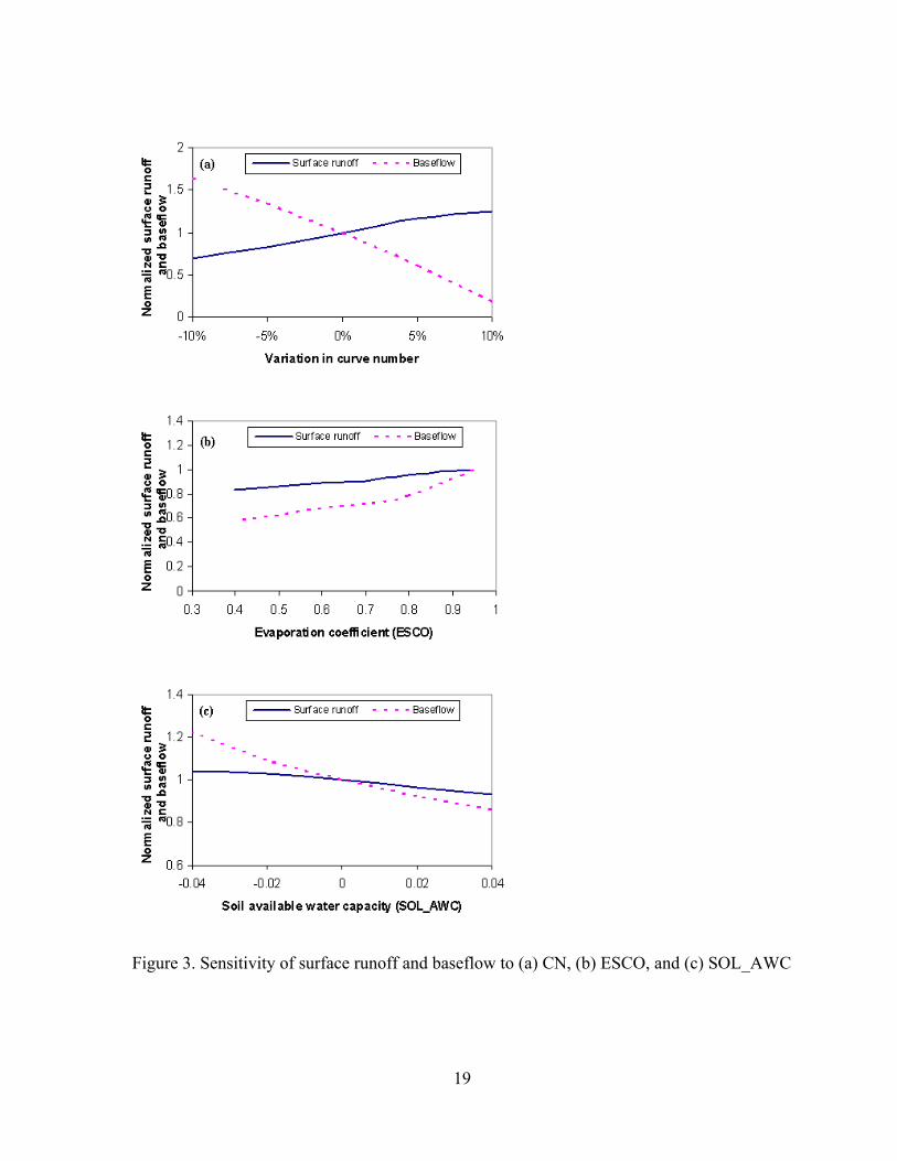
The top three most influencing parameters were CN, ESCO, and SOL_AWC. A further

detailed sensitivity analysis was performed for these three parameters. CN was found to be

extremely sensitive parameter for flow. CN is a dimensionless number that is related to land

use and soil type. Figure 3(a) shows the response of surface runoff and baseflow when CN

11

was changed from -10% to +10%. Larger CN values resulted in increased surface runoff and

at the same time decreased infiltration. Baseflow is inversely proportional to CN. The second

most sensitive parameter, ESCO, was found to have more impact on baseflow than on

surface runoff (Figure 3b). ESCO adjusts the depth distribution for evaporation from the soil

to account for the effect of capillary action, crusting, and cracking. Decreasing ESCO allows

lower soil layers to compensate for a water deficit in upper layers and causes higher soil

evapotranspiration, which in turn reduces both surface runoff and baseflow. Figure 3c shows

the sensitivity of the model to SOL_AWC. Increasing SOL_AWC was found to lead to

higher soil water capacity, which increased both surface runoff and baseflow. Conversely,

decreasing soil water capacity resulted in higher water availability for surface runoff and

baseflow.

3.2 Calibration and validation

The SWAT model was calibrated and validated for streamflow using the measured data

at USGS gage station 05418500 (Maquoketa River near Maquoketa, Iowa). The measured

data was divided into two parts: 1988 to 1993 for calibration and 1982 to 1987 for validation.

The calibration period includes wide variation of climatic conditions of wet, dry, and normal

years. During the calibration process, the model’s input parameters were adjusted, as guided

by the sensitivity analysis, to match the observed and simulated streamflows. Table 3 lists the

final calibrated values of the model variables. A time-series plot of the measured and

simulated monthly streamflows (Figure 4) shows that the magnitude and trend in the

simulated monthly flows closely followed the measured data most of the time. The measured

and simulated average monthly flow volumes were 22.28 and 24.08 mm, respectively. The

12

statistical evaluation yielded an R2 value of 0.86 and an E value of 0.85, indicating a strong

correlation between the measured and predicted flows.

Flow validation was conducted using the streamflow data for the period 1982 to 1987. In

the validation process, the model was run with input parameters set during the calibration

process without any change. Figure 5 shows the time-series plot of monthly measured and

simulated monthly streamflows and indicates an acceptable correspondence of simulated

streamflows with the measured values. The measured and simulated average monthly flow

volumes for the validation period were 23.40 and 23.44 mm, respectively. The R2 and E

values between the measured and simulated streamflows were 0.69 and 0.61, respectively.

Overall, it can be concluded that the model was able to predict streamflow with reasonable

accuracy.

4. Conclusion

Information about a model’s sensitivity to some input parameters benefits model

development and leads to the model’s successful application. This study identified which

input hydrologic parameters the SWAT model is most sensitive to using the influence

coefficient method, as determined in an application to the Maquoketa River watershed.

Surface runoff was found to be sensitive, from most to least, to CN, ESCO, SOL_AWC, and

EPCO for the selected variation range, while baseflow was found to be sensitive, from most

to least, to CN, ESCO, SOL_AWC, RECHRG_DP, GW_REVAP, ALPHA_BF, and

GW_DELAY. Surface runoff was found to be not sensitive at all to ALPHA_BF,

GW_REVAP, GW_DELAY, and RECHARG_DP, while baseflow was found to be sensitive

to all the parameters chosen in this study. Model sensitivities to the three most influencing

13

parameters for both surface runoff and baseflow—CN, ESCO, and SOL_AWC—were

further evaluated. Sensitivity analysis provides good insight into the model input parameters

and demonstrates that the model is able to simulate hydrological processes very well.

Based on the assessment of model parameters to which the model is most to least

sensitive, SWAT was calibrated and validated for streamflow at the watershed outlet. The

calibration process used measured data for the period 1988-1993 and yielded a strong

correlation (R2 = 0.86 and E = 0.85) between measured and simulated flow volumes. Model

validation was performed for the period 1982-1987 and generated an R2 value of 0.69 and E

value of 0.61. This study indicates that the SWAT model can be an effective tool for

accurately simulating the hydrology of the Maquoketa River watershed. Accurate flow

simulations are required to accurately predict sediment loads and chemical concentrations,

and to simulate various scenarios related to cropping and alternative management to mitigate

water quality problems in the region.

14

References

Arnold, J.G., Allen, P.M., 1996. Simulating hydrologic budgets for three Illinois watersheds. Journal of Hydrology 176, 57-77.

Arnold, J.G., Muttiah, R.S., Srinivasan, R., Allen, P.M., 2000. Regional estimation of base

flow and groundwater recharge in the Upper Mississippi River Basin. Journal of Hydrology 227, 21-40.

Arnold, J.G., Srinivasan, R., Muttiah, R.S., Allen, P.M., Walker, C., 1999. Continental scale

simulation of the hydrologic balance. Journal of American Water Resources Association 35(5), 1037-1052.

Arnold, J.G., Srinivasan, R., Muttiah, R.S., Williams, J.R., 1998. Large area hydrologic

modeling and assessment Part I: Model development. Journal of American Water Resources Association 34(1), 73-89.

Arnold, J.G., Williams, J.R., Nicks, A.D., Sammons, N.B., 1990. SWRRB: A basin scale

simulation model for soil and water resources management. Texas A & M University Press, College Station, Texas.

Di Luzio, M., Srinivasan, R., Arnold, J.G., Neitsch, S.L., 2000. Soil and Water Assessment

Tool: ArcView GIS Interface Manual, Version 2000. Texas Water Resources Institute TR-193, GSWRL 02-03, BRC 02-07, 345 pages.

FitzHugh, T.W., Mackay, D.S., 2000. Impacts of input parameter spatial aggregation on an

agricultural nonpoint source pollution model. Journal of Hydrology 236(1-2), 35-53. Gassman, P.W., Reyes, M., Green, C.H., Arnold, J.G., 2007. The Soil and Water Assessment

Tool: Historical development, applications, and future directions. Transactions of the ASABE 50(4), 1211-1250.

Gu, R., Li, Y., 2002. River temperature sensitivity to hydraulic and meteorological

parameters. Journal of Environmental Management 66(1), 43-56. Helsel, D.R., Hirsch, R.M., 1992. Statistical Methods in Water Resources. Elsevier, New

York. Jha, M., Gassman, P.W., Secchi, S., Gu, R., Arnold, J.G., 2004a. Effect of watershed

subdivision on SWAT flow, sediment, and nutrient predictions. Journal of American Water Resources Association 40(3), 811-825.

Jha, M., Pan, Z., Takle, E.S., Gu, R., 2004b. Impacts of climate change on streamflow in the

Upper Mississippi River Basin: A regional climate model perspective. Journal of Geophysical Research 109:D09105.

15

Johansen, N.B., Imhoff, J.C., Kittle, J.L., Donigian, A.S., 1984. Hydrologic simulation

program - FORTRAN (HSPF): User’s Manual for release 8, EPA-600/3-84-066, Athens, GA, U.S. Environmental Protection Agency.

Knisel, W.G., ed., 1980. CREAMS: A Field-Scale Model for Chemicals, Runoff, and

Erosion from Agricultural Management Systems. Conservation Research Report No. 26, Washington, D.C.: USA-SEA.

Lenhart, T., Eckhardt, K., Fohrer, N., Frede, H.-G., 2002. Comparison of two different

approaches of sensitivity analysis. Physics and Chemistry of the Earth 27, 645-654. Neitsch, S.L., Arnold, J.G., Kiniry, J.R., Williams, J.R, 2002. Soil and Water Assessment

Tool Theoretical Documentation, Version 2000 (Draft). Blackland Research Center, Texas Agricultural Experiment Station, Temple, Texas.

Saleh, A., Arnold, J.G., Gassman, P.W., Hauck, L.M., Rosenthal, W.D., Williams, J.R.,

McFarland, A.M.S., 2000. Application of SWAT for the Upper North Bosque River watershed. Transactions of the ASAE 43(5), 1077-1087.

Santhi, C., Arnold, J.G., Williams, J.R., Dugas, W.A., Srinivasan, R., Hauck, L.M., 2001.

Validation of the SWAT Model on a large river basin with point and nonpoint sources. Journal of American Water Resources Association 37(5), 1169-1188.

Spruill, C.A., Workman, S.R., Taraba, J.L., 2000. Simulation of daily and monthly stream

discharge from small watershed using the SWAT Model. Transactions of the ASAE 43(6), 1431-1439.

Srinivasan, R., Ramanarayanan, T.S., Arnold, J.G., and Bednarz, S.T., 1998. Large area

hydrologic modeling and assessment, Part II: Model application. Journal of American Water Resources Association 34(1), 91-102.

Stone, M.C., Hotchkiss, R.H., Hubbard, C.M., Fontaine, T.A., Mearns, L.O., Arnold, J.G.,

2001. Impacts of climate change on Missouri River basin water yield. Journal of American Water Resources Association 37(5), 1119-1130.

U.S. Army Corps of Engineers Hydrologic Engineering Center (USACE-HEC), 2002. HEC-

HMS Hydrologic Modeling System user’s manual, USACE-HEC, Davis, Calif. U.S. Department of Agriculture (USDA), 1994. State Soil Geographic (STATSGO) Data

Base: Data Use Information. Misc. Publication Number 1492, Natural Resource Cons. Service. National Soil Survey Center, Lincoln, Nebraska.

16

U.S. Environmental Protection Agency (USEPA), 2001. BASINS 3.0: Better Assessment Science Integrating Point and Nonpoint Sources. U.S. Environmental Protection Agency, Office of Water, Office of Science and Technology, Washington, D.C.

Whittemore, R.C., 1998. The BASINS Model. Water Environment and Technology 10:57-

61. Williams, J.R., Jones, C.A., Dyke, P.T., 1984. A modeling approach to determining the

relationship between erosion and soil productivity. Transactions of the ASAE 27, 129-144.

Young, R.A., Onstad, C.A., Bosch, D.D., Anderson, W.P., 1989. AGNPS: A non-point

source pollution model for evaluating agricultural watersheds. Journal of Soil and Water Conservation 44(2), 168-173.

17

Figure 1. Location of the Maquoketa River watershed (Northeast Iowa), and weather stations

 

18

Figure 2. Land use categories in Maquoketa River watershed

19

Figure 3. Sensitivity of surface runoff and baseflow to (a) CN, (b) ESCO, and (c) SOL_AWC

20

Figure 4. Monthly time series of predicted and measured streamflow at USGS gauge

05418500 (watershed outlet) for the 1988-93 calibration period

21

Figure 5. Monthly time series of predicted and measured streamflow at USGS gauge

05418500 (watershed outlet) for the 1982-87 validation period

22

Table 1. Parameter ranges and initial values used in the sensitivity analysis

Model parameter* Variable name Range Model initial

estimates

Curve Number (for AGRL) CN 69-85 77

Soil evaporation compensation factor ESCO 0.75-0.95 0.95

Plant uptake compensation factor EPCO 0.01-1 1.0

Soil available water capacity (mm) SOL_AWC ±0.04 -

Baseflow alpha factor ALPHA_BF 0.05-0.8 0.048

Groundwater revap coefficient GW_REVAP 0.02-0.2 0.02

Groundwater delay time (day) GW_DELAY 0-100 31

Deep aquifer percolation fraction RECHRG_DP 0-1 0.05

*Detailed descriptions are given in the SWAT theoretical documentation (Neitsch et al.,

2002).

23

Table 2. Sensitivity indices of model parameters

Parameter Initial value

Parameter Response variable (Surface Runoff) Response variable (Baseflow)

P1 P2 ΔP Mean (Pm) F1 F2 ΔF Mean

Fm PF

ΔΔ

PF

FP

m

m

ΔΔ F1 F2 ΔF Mean

Fm PF

ΔΔ

PF

FP

m

m

ΔΔ

CN 77 85 69 16 77 310 173 137 241 8.57 2.73 21 181 -160 101 -10.0 -7.63

ESCO 0.95 0.5 1 0.5 0.75 214 249 -34 231 -68.9 -0.22 69 110 -41 90 -82.2 -0.69

EPCO 1 0.01 1 0.99 0.505 264 249 15 256 15.09 0.03 124 110 14 117 14.1 0.06

SOL_AWC 0.04 -0.04 0.08 0.04 232 259 -27 246 -336 -0.05 95 135 -40 115 -503 -0.17

ALPHA_BF 0.048 0.048 0.8 0.75 0.424 249 249 0 249 0 0 110 114 -4 112 -4.7 -0.02

GW_REVAP 0.02 0.02 0.2 0.18 0.11 249 249 0 249 0 0 110 95 15 102 85.6 0.09

GW_DELAY 31 0 100 100 50 249 249 0 249 0 0 108 106 1 108 0.0 0.01

RECHARG_DP 0.05 0 1 1 0.5 249 249 0 249 0 0 113 91 22 102 22.3 0.11

24

Table 3. Final calibrated values of SWAT parameters for Maquoketa River watershed

Parameter Value

CN (for AGRL only) 72

ESCO 0.85

SOL_AWC -0.04

GW_REVAP 0.15

GW_DELAY 50

RECHRG_DP 0.5