Hydrologic Modeling of the Court Creek Watershed calibration and verification runs demonstrated that...

Contract Report 2000-04

Hydrologic Modeling of the Court Creek Watershed

byDeva K. Borah and Maitreyee Bera

Prepared for theIllinois Department of Natural Resources

March 2000

Illinois State Water SurveyWatershed Science SectionChampaign, Illinois

A Division of the Illinois Department of Natural Resources

Hydrologic Modeling of the Court Creek Watershed

by

Deva K. Borah and Maitreyee Bera

Illinois State Water SurveyWatershed Science Section

2204 Griffith DriveChampaign, Illinois 61820-7495

A Division of the Office of Scientific Research and AnalysisIllinois Department of Natural Resources

Prepared for theIllinois Department of Natural Resources

Watershed Management SectionOffice of Resource Conservation

524 South Second StreetSpringfield, Illinois 62701

IDNR Contract Number: G99C0230

March 2000

ISSN 0733-3927

This report was printed on recycled and recyclable papers.

ii

Executive Summary

Flooding, upland soil and streambank erosion, sedimentation, and contaminationof drinking water from agricultural chemicals (nutrients and pesticides/herbicides) arecritical environmental problems in Illinois. Upland soil erosion causes loss of fertile soil,streambank erosion causes loss of valuable riparian lands, and both contribute largequantities of sediment (soil and rock particles) in the water flowing through streams andrivers, which causes turbidity in sensitive biological resource areas and fills water supplyand recreational lakes and reservoirs. Most of these physical damages occur duringsevere storm and flood events. Eroded soil and sediment also carry chemicals that pollutewater bodies and stream/reservoir beds.

Court Creek and its 97-square-mile watershed in Knox County, Illinois,experience problems with flooding and excessive streambank erosion. Several fish killsreported in the streams of this watershed were due to agricultural pollution. Because ofthese problems, the Court Creek watershed was selected as one of the pilot watersheds inthe Illinois multi-agency Pilot Watershed Program (PWP). The watershed is located inenvironmentally sensitive areas of the Illinois River basin; therefore, it is also part of theIllinois Conservation Reserve Enhancement Program (CREP).

Understanding and addressing the complex watershed processes of hydrology,soil erosion, transport of sediment and contaminants, and associated problems have beena century old challenge for scientists and engineers. Mathematical computer modelssimulating these processes are becoming inexpensive tools to analyze these complexprocesses, understand the problems, and find solutions through land-use changes and bestmanagement practices (BMPs). Effects of land-use changes and BMPs are analyzed byincorporating these into the model inputs. The models help in evaluating and selectingfrom alternative land-use and BMP scenarios that may help reduce damaging effects offlooding, soil and streambank erosion, sedimentation (sediment deposition), andcontamination to the drinking water supplies and other valuable water resources.

A computer model of the Court Creek watershed is under development at theIllinois State Water Survey (ISWS) using the Dynamic Watershed Simulation Model(DWSM) to help achieve the restoration goals set in the Illinois PWP and CREP bydirecting restoration programs in the selection and placement of BMPs. The current studyis part of this effort. The DWSM uses physically based governing equations to simulatepropagation of flood waves, entrainment and transport of sediment, and commonly usedagricultural chemicals for agricultural and rural watersheds. The model has three majorcomponents: (1) hydrology, (2) soil erosion and sediment transport, and (3) nutrient andpesticide transport. The hydrologic model of the Court Creek watershed was developedusing the hydrologic component of the DWSM, which is the basic (foundation)component simulating rainfall-runoff on overland areas, and propagation of flood wavesthrough an overland-stream-reservoir network of the watershed. A new routine wasintroduced into the model to allow simulation of spatially varying rainfall eventsassociated mainly with moving storms and localized thunderstorms. The model wascalibrated and verified using three rainfall-runoff events monitored by the ISWS.

iii

The calibration and verification runs demonstrated that the model wasrepresentative of the Court Creek watershed by simulating major hydrologic processesand generating hydrographs with characteristics similar to the observed hydrographs atthe monitoring stations. Therefore, model performance was promising consideringwatershed size, complexities of the processes being simulated, limitations of availabledata for model inputs, and model limitations. The model provides an inexpensive tool forpreliminary investigations of the watershed for illustrating the major hydrologicprocesses and their dynamic interactions within the watershed, and for solving some ofthe associated problems using alternative land use and BMPs, evaluated throughincorporating these into the model inputs.

The model was used to compare flow predictions based on spatially distributedand average rainfall inputs and no difference was found because of a fairly uniformrainfall pattern for the simulated storm. However, the routine will be useful forsimulating moving storms and localized thunderstorms. A test to examine effects ofdifferent watershed subdivisions with overland and channel segments found no differencein model predictions. This was because of the dynamic routing schemes in the modelwhere dynamic behaviors were preserved irrespective of the sizes and lengths of thedivided segments. Although finer subdivision does not add accuracy to the outflows, itallows investigations of spatially distributed runoff characteristics and distinguishes theseamong smaller areas, which helps in prioritizing areas for proper attention andrestoration.

The calibrated and verified model was used to simulate four synthetic (design)storms to analyze and understand the major dynamic processes in the watershed. Detailedsummaries of results from these model runs are presented. These summary results wereused to rank overland segments based on unit-width peak flows, which indicatedpotential flow strengths that may damage the landscape, and were based on runoffvolumes that indicate potential flood-causing runoff amounts. Stream channel andreservoir segments also were ranked based on peak flows and indicate potential fordamages to the streams. Maps were generated showing these runoff potentials ofoverland areas. These results may be useful in identifying and selecting critical overlandareas and stream channels for implementation of necessary BMPs to control damagingeffects of runoff water.

The model also was used to evaluate and quantify effects of the two major lakesin the watershed in reducing downstream flood flows and demonstrating model ability toevaluate detention basins. The model was run for one of the design storms with andwithout the lakes. The results showed significant reduction of peak flows and delaying oftheir occurrences immediately downstream. These effects become less pronouncedfurther downstream.

This report presents and discusses results from the above applications of theDWSM hydrology to the Court Creek watershed along with descriptions of the

iv

watershed, formulations of the hydrology component of the DWSM, limitations of themodel and available data affecting predictions, and recommendations for future work.

Efforts are currently under way at the ISWS to add subsurface and tile flowroutines to the DWSM that would improve model predictions and their correspondencewith observed data. It is recommended that stream cross-sectional measurements be madeat representative sections of all major streams in the Court Creek watershed and thatstream flow monitoring be continued or established at least at outlets of major tributariesand upper and lower Court Creek. A minimum of four equally spaced raingage stationsare recommended for recording continuous rainfall.

v

vi

CONTENTS

Page

Introduction 1 Acknowledgments 5

Court Creek Watershed and Its Investigations 6

The Hydrologic Component of DWSM 9

Modeling the Court Creek Watershed 15 Simulation of April 1, 1983, Storm: Model Calibration 16 Simulation of December 24, 1982, Storm: Model Verification 18 Simulation of December 2, 1982, Storm: Model Verification 19 Effect of Spatially Distributed Rainfall Data 21 Simulations of Design Storms 21 Runoff Potentials in Overland Areas, Streams, and Reservoirs 24 Impacts of Detention Basins 33 Effect of Different Watershed Subdivisions 36

Conclusions 39

References 41

Appendix A. Hydrology Formulations Used in the Dynamic Watershed Simulation Model 45

Appendix B. Model Results for Design Storms 51

vii

LIST OF FIGURES

Page

1. Location, topography, and major physical features of the Court Creek watershed 3

2. Major streams, reservoirs, streamgages, and raingages in the Court Creek watershed 7

3. Numbering of model segments in the Court Creek watershed 10

4. Dynamic Watershed Simulation Model approximations of overland and channel segments 11

5. Dynamic Watershed Simulation Model overland and channel flow approximations 12

6. Flow diagram of Dynamic Watershed Simulation Model hydrologic simulation 13

7. Comparisons of predicted and observed water discharges in the Court Creek watershed resulting from the (a) April 1, 1983, storm: model calibration and the (b) December 24, 1982, storm: model verification 17

8. Comparisons of predicted and observed water discharges in the Court Creek watershed resulting from the (a) December 2, 1982, storm: model verification and the (b) April 1, 1983, storm showing effect of distributed and averaged rainfall 20

9. Comparisons of predicted water discharges in the Court Creek watershed resulting from design storms in western Illinois and Soil Conservation Service rainfall distributions: (a) Middle Creek, North Creek, and outflow from 1-year, 24-hour rainfall; (b) outflows from 2-year, 6-hour; 10-year, 6-hour; 1-year, 24-hour; and 2-year, 24-hour rainfall 23

10. Runoff potentials of overland areas in Court Creek watershed based on unit-width peak flows 27

11. Runoff potentials of overland areas in Court Creek watershed based on runoff volumes 31

viii

LIST OF FIGURES (concluded)

Page

12. Comparisons of water discharges in Court Creek watershed resulting from a 1-year, 24-hour rainfall in western Illinois and Soil Conservation Service rainfall distribution showing impact of lakes: (a) inflows to and outflows from Rice Lake, (b) inflows to and outflows from Spoon Valley Lake, and (c) watershed outflows with and without Spoon Valley Lake 35

13. Coarse model divisions of the Court Creek watershed 37

14. Comparisons of predicted and observed outflows from the Court Creek watershed for the April 1, 1983, storm showing effect of fine and coarse divisions of the watershed 38

ix

TABLES

Page

1. Ranking of Overland Segments of Court Creek Watershed Based on Unit-Width Peak Flows in Descending Order Resulting from Design Storms 25

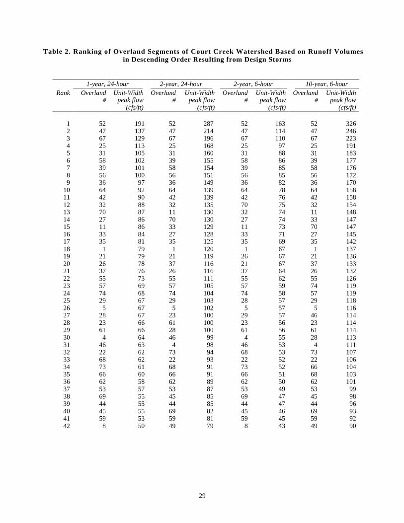
2. Ranking of Overland Segments of Court Creek Watershed Based on Runoff Volumes in Descending Order Resulting from Design Storms 29

3. Ranking of Stream and Reservoir Segments of Court Creek Watershed Based on Peak Flows in Descending Order Resulting from Design Storms 34

Introduction

Flooding, upland soil and stream bank erosion, sedimentation, and contaminationof drinking water from agricultural chemicals (nutrients and pesticides/herbicides) arecritical environmental problems in Illinois (Roseboom et al., 1982a; Fitzpatrick et al.,1985, 1987; Demissie et al., 1988, 1992, 1996; Mitchell et al., 1994; Keefer et al., 1996;Goolsby et al., 1999). Upland soil erosion causes loss of fertile soil, streambank erosioncauses loss of valuable riparian lands, and both contribute large quantities of sediment(soil and rock particles) to the water flowing through streams and rivers causing turbidityin sensitive biological resource areas and filling water supply and recreational lakes andreservoirs. A few examples of serious lake sedimentation in Illinois are Lake Decatur(Fitzpatrick et al., 1987), Lake Springfield (Fitzpatrick et al., 1985), and Peoria Lake(Demissie et al., 1988). Most of these physical damages occur during severe storm andflood events. Eroded soil and sediment also carry chemicals that pollute water bodies andstream/reservoir beds.

Court Creek and its watershed in Knox County, Illinois, experience problems withflooding and excessive streambank erosion (Roseboom et al., 1982a). Several fish kills,including an extensive fish kill in 1981, reported in the streams of this watershed weredue to agricultural pollution. Because of these problems in this 97-square-mile watershed(Figure 1), the Court Creek watershed was selected as one of the pilot watersheds inIllinois. The watershed, located in environmentally sensitive areas of the Illinois Riverbasin, is also part of the Illinois Conservation Reserve Enhancement Program (CREP).

The Pilot Watershed Program (PWP), established in 1998, is an interagency effortto promote coordination between government agencies and local communities, and toimplement watershed science principles and good management practices on fourwatersheds in Illinois. Program goals are to understand watershed processes and developland-use management tools that reduce soil and streambank erosion, improve waterquality in streams and lakes, and increase the abundance of a variety of aquatic andterrestrial species. Participating agencies include: Illinois Department of NaturalResources (IDNR), Illinois Department of Agriculture (IDOA), Illinois EnvironmentalProtection Agency (IEPA), U.S. Department of Agriculture (USDA) Natural ResourcesConservation Service (NRCS), Association of Illinois Soil and Water ConservationDistricts (AISWCD), and Farm Service Agency (FSA). The four pilot watersheds areCourt Creek, Hurricane Creek, Sugar Creek, and Big Creek located in the Spoon,Embarras, Kaskaskia, and Cache River basins, respectively. The PWP is described brieflyin a document circulated jointly by the participating agencies (IDOA et al., 1998).

The CREP, a state and federal partnership program, was launched in 1998 topromote cleaner land and waters along the Illinois River (Thomas, 1998). Goals of thisprogram are to reduce sedimentation and nutrients in the Illinois River by 20 and 10percent, respectively; increase populations of waterfowl, shorebirds, nongame grasslandbirds, and threatened/endangered species by 15 percent; and increase the native fish andmussel population in the lower reaches of the Illinois River by 10 percent. The CREP is

1

part of a much older and bigger federal program called the Conservation ReserveProgram (CRP), which was designed to remove environmentally sensitive farmlandsfrom production. The Illinois CREP expands on CRP through a partnership with the stateand provides additional incentives for landowners to voluntarily enter into an agreementto extend the CRP contract. The program focuses on the Illinois River from Meredosia toStarved Rock, plus tributaries to the river, including the Spoon, Mackinaw, Vermilion,Kankakee, lower Fox, and lower Sangamon Rivers. Court Creek, a tributary to the SpoonRiver, is part of the program. The FSA manages the federal part of the program. TheIDNR has the primary responsibility for administering the fiscal portion of the state partof the program and works with other federal and state agencies, including IDOA, IEPA,and local Soil and Water Conservation Districts, in implementing the program.

Understanding and addressing the complex processes of hydrology, soil erosion,transport of sediment and contaminants, and associated problems have been a century oldchallenge for scientists and engineers, especially due to the spatial and temporalvariability of those processes within a watershed. Mathematical (computer) modelssimulating these processes are becoming inexpensive tools to analyze those complexprocesses, understand the problems, and find solutions through land-use changes and bestmanagement practices (BMPs). Effects of land-use changes and BMPs are analyzed byincorporating these into the model inputs. The models help in evaluating and selectingfrom alternative land-use and BMP scenarios, implementation of which may help reducedamaging effects of flooding, soil and streambank erosion, sedimentation (sedimentdeposition), and contamination to the drinking water supplies and other valuable waterresources.

A dynamic watershed simulation model (DWSM) is being developed at theIllinois State Water Survey (ISWS) (Borah et al., 1998, 1999a, b) using physically basedgoverning equations to simulate propagation of flood waves, entrainment and transport ofsediment, and commonly used agricultural chemicals for agricultural and ruralwatersheds. The model has three major components: (1) hydrology, (2) soil erosion andsediment transport, and (3) nutrient and pesticide transport. Formulations and proceduresof these components are adopted from earlier work of the first author (Borah, 1989a, b;Ashraf and Borah, 1992). Each of these model components has efficient routing schemesbased on approximate analytical solutions of the physically based governing equations,and preserving the dynamic behaviors of the water, sediment, and accompanyingchemical movements. The model has been tested on the 925-square-mile UpperSangamon River basin in east central Illinois, draining into Lake Decatur, usingmonitored data (Borah et al., 1998, 1999a, b).

A computer model of the Court Creek watershed is under development at theISWS using its DWSM to help achieve the restoration goals set in the Illinois PWP andCREP, i.e., to guide restoration programs in the selection and placement of BMPs. Thecurrent study is part of this effort. The hydrologic model of the watershed is developedusing the hydrologic component of the DWSM, which is the basic (foundation)component simulating storm water rainfall-runoff on overland areas and propagation offlood waves through an overland-stream-reservoir network of the watershed.

2

Figure 1. Location, topography, and major physical featuresof the Court Creek watershed

3

Extensive hydrologic, land-use, water quality, and biological data were collectedon the Court Creek watershed by the ISWS during 1980-l988 (Roseboom et al., 1982a, b,1986, 1990). These data were used to develop the basic model inputs. Using the rainfall-runoff data of three monitored storms, the model was calibrated and verified and thenused to simulate four synthetic or design storms. The results were used to determinerunoff potentials of overland, stream channel, and reservoir segments. One storm wasused to evaluate impacts of the two existing lakes and demonstrate use of detention pondsas a BMP for reducing downstream flood flows that may have impacts on flood damagesand streambank erosion.

This report presents and discusses results from the applications of the DWSM tothe Court Creek watershed, descriptions of the watershed, formulations of the hydrologycomponent of DWSM, limitations of the model and the available data affectingpredictions, and recommendations for future work.

Acknowledgments

The authors acknowledge the financial support from IDNR to conduct this study.They sincerely appreciate the support, cooperation, and enthusiasm from DouglasAusten, head of the Watershed Management Section, Office of Resource Conservation,IDNR; David Day; and their colleagues while initiating the study as well as during thecourse of the study.

Partial funding was from the Illinois Council on Food and Agricultural Research(C-FAR) Water Quality Strategic Research Initiative (WQ-SRI) Program. The authorsthank Mark Godsil, chairman of the Court Creek Watershed Planning Committee, andJames Westervelt, coordinator of the C-FAR WQ-SRI modeling program for theirinterest, enthusiasm, and encouragement. The findings and recommendations in thisreport are not necessarily those of the funding agencies or of the Illinois State WaterSurvey.

The authors wish to express their sincere appreciation to Donald Roseboom ofISWS for his generous support to this study by giving the authors a comprehensive fieldtour of the Court Creek watershed, providing them with published reports, storm rainfalland flow data, and valuable guidance during the study.

The authors thank ISWS Chief Derek Winstanley and Watershed Science Sectionhead Nani Bhowmik (former) and Manoutchehr Heidari (interim) for their support andpermission to use ISWS resources in initiating, expanding, and completing this basic partof the Court Creek watershed modeling study. They specially thank Chief Winstanley forhis critical and useful comments on the report. They also thank Kathleen Brown for herassistance in preparing the Geographic Information System maps and Renjie Xia andSusan Shaw for critically reviewing the report. Eva Kingston and Agnes Dillon edited thereport, and Linda Hascall reviewed and formatted the graphics.

5

Court Creek Watershed and Its Investigations

The Court Creek watershed is located in Knox County, east of Galesburg, Illinois.Figure 1 shows the boundaries, topography, and major physical features of this 97-square-mile (251-square-kilometer or 62,000-acre) watershed, drawn based on U.S.Geological Survey 7.5-Minute Series Topographic Quadrangle maps. The watershed liesalmost entirely within the four townships of Knox, Sparta, Copley, and Persifer. CourtCreek flows along the southern boundary of the watershed for 14.5 miles beforedischarging into the Spoon River, a western tributary of the Illinois River, at Dahinda.Three major tributaries, Middle Creek, North Creek, and Sugar Creek, enter Court Creekfrom the north. Strip mining created numerous small lakes over a 3,400-acre area in theupper Sugar Creek basin. Directly below the strip-mined lands, a 512-acre Spoon ValleyLake impounds the waters of Sugar Creek for the Oak Run housing development. Theonly other lake in the watershed is Rice Lake, a 30-acre impoundment on the upper endof Court Creek.

Roseboom et al. (1982a, b, 1986, 1990) collected extensive hydrologic, land-use,and water quality data on the Court Creek watershed during 1980-1988. Land use in thewatershed is predominately agriculture with row crop fields occurring on 49 percent ofthe watershed. More than 70 percent of the row crop acreage is corn. Pastures, woodedpastures, and strip-mine pastures are on 29 percent of the watershed. Animal feedlotsoccur on 0.3 percent of the watershed and contain the majority of the 60,000 livestockpresent in the watershed. Fifteen of the 93 feedlots in the watershed are total confinementsites. Urban areas in the watershed include Galesburg and a portion of Knoxville (Figure1). The watershed has two county landfills.

Thirty-nine percent of the land in the Court Creek watershed has slopes greaterthan a 15 percent grade. These lands are normally in pasture, wooded pasture, strip-minepasture, and woods. Less than 6 percent of the watershed has slopes between 6 and 15percent. More than 50 percent of the watershed has slopes less than a 6 percent grade.Watershed areas with less than a 6 percent slope have been used for row crop agricultureand residential housing.

Roseboom et al. (1982a) reported detailed physical, soil, land-use, hydrologic,and hydraulic characteristics and data of the Court Creek watershed and its streams. Ninemajor bank erosion sites along Court Creek were examined, and soil composition of thebanks and some chemical characteristics were analyzed. Bank erosion sites along NorthCreek also were identified and analyzed. Extensive monitoring stations were establishedto monitor rainfall (13 stations), flow (9 stations), and water quality parameters (9primary and 7 supplemental stations). Figure 2 shows some of the stream and all theraingage stations. Data from these stations were used in the modeling study. In the firstmonitoring investigation of Roseboom et al. (1982a), monitoring was conducted during1980-1982. In a separate report, Roseboom et al. (1982b) reported all the monitored dataon rainfall, flow, water quality, and fish survey. The investigators reported a pesticidefish kill in the Spoon Valley Lake in 1981.

6

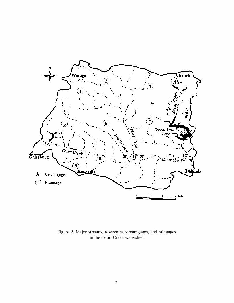
Figure 2. Major streams, reservoirs, streamgages, and raingagesin the Court Creek watershed

7

In a subsequent investigation, Roseboom et al. (1986) studied the influences ofland uses and stream modifications on water quality in the streams of the Court Creekwatershed. Additional data on rainfall, flow, sediment, water quality, and streambankerosion were collected during December 1982-April 1983 storms.

Roseboom et al. (1990) conducted another monitoring study during the droughtyears of 1987 and 1988. Data collected during 1986 also were reported. Water qualityparameters of both nutrient and pesticides were collected during baseflow and stormrunoff conditions. Contributions from row crops and feedlots were investigated.

Enormous hydrologic, hydraulic, water quality, and biological (fisheries) datawere collected on the Court Creek watershed. Due to its geographical location and theavailable data, this watershed was selected as one of the four pilot watersheds in Illinois,and played a key role in the interagency PWP and CREP, which were supported byConservation 2000 funds. The watershed has a standing committee, the Court CreekWatershed Planning Committee (CCWPC), with high local interest.

Extensive investigations and future research planning are underway on the CourtCreek and other pilot watersheds. State staff, state and university researchers, and localwatershed representatives have been meeting regularly to discuss the status of watershedscience, watershed assessment, future research, support, and coordination on the pilotwatersheds (Austen and Hogan, 1999a, b). Emphasis was given to improvedcommunication between landowners, agency staff, and researchers toward the commongoal of restoring watersheds. These efforts have generated several research projects byuniversity and state researchers, planning grants to the local watershed groups, activewatershed planning committees, and considerable interest in watershed issues. The CourtCreek modeling study presented in this report is part of these efforts.

8

The Hydrologic Component of DWSM

The driving force of DWSM comes from a dynamic hydrologic model in whichhydrologic processes are simulated for a given rainfall event, and time and space varyingflow depths and flow rates of surface runoff are computed. These processes are simulatedby dividing the watershed into subwatersheds, specifically, into one-dimensionaloverland, channel, and reservoir flow elements or segments (Figure 3). The Court Creekwatershed was divided into 78 overland, 39 channel, and 2 reservoir segments, which areidentified by numbers: 1-78 (overland), 79-117 (channel), and 118-119 (reservoir). Thesedivisions take into account the nonuniformities in topographic, soil, and land-usecharacteristics, which are treated as being uniform within each of the segments.

The overland segments are represented by rectangular areas with representativelength, slope, width, soil, cover, and roughness. The channels are described byrepresentative cross-sectional shape, slope, length, and roughness. The reservoirs arerepresented by stage-storage-discharge relations. Figure 4 shows model approximationsof six overland segments (1-6) contributing to three channel segments (79-81). Areas ofthe overland and lengths of the channel segments are measured in the dividedtopographic map (Figure 3). Width (W in Figure 4) of a model overland (1) is equal tothe length of the receiving channel (79). Length (L) of the model overland (1) iscomputed by dividing its area by the length of the receiving channel (79).

The overland segments are the primary sources of runoff (flowing water) in whichrainfall turns into runoff after losses first to interception at canopies and ground covers,then to infiltration through the soil matrix and depression storage on the ground surface.The rainfall available for runoff is referred to as rainfall excess. Two overland segmentscontribute to one channel segment laterally from each side of the channel as shown inFigure 5. The excess rainfall is routed over the overland segments beginning at theirupstream edges (ridges), in which flows are zeros, up to their downstream edges,coinciding with the receiving channel banks. Because the physical and meteorologicalcharacteristics of an overland segment are assumed uniform, routing of excess rainfallover only a unit width resulting in “flow per unit width” of the segment is required. Theunit-width flow is uniform along the overland width and discharges uniformly along thechannel length. Figure 5 will be discussed further along with introduction of the variablesin Appendix A and the overland and channel flow routing scheme. The channels carry thereceiving water downstream of the watershed and ultimately to the watershed outlet.During its journey, the runoff water may be intercepted by lakes or reservoirs, whichrelease it again to downstream channels at reduced rates after temporary storage.

Figure 6 shows the general computational operations of the DWSM-hydrologiccomponent in the form of a flow diagram. Rates of rainfall excess on the overlandelements are computed from a given breakpoint rainfall record (rainfall recorded atdifferent times during a storm) using two alternative algorithms. The method used in thisstudy is the Soil Conservation Service (SCS) runoff curve number method described in

9

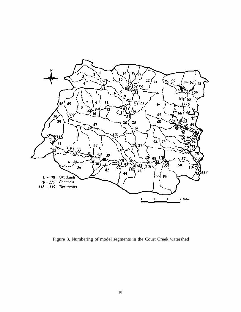
Figure 3. Numbering of model segments in the Court Creek watershed

10

Figure 4. Dynamic Watershed Simulation Model approximationsof overland and channel segments

11

Figure 5. Dynamic Watershed Simulation Model overlandand channel flow approximations

12

INPUT

l Overland Datal Channel Datal Reservoir Datal Computational Sequencel Precipitation Data

OVERLAND RESERVOIRFlow Unit

?

l Time varyingrainfall excessby SCS curve numberor interception-infiltration method

l Flow routing byanalytical and shock-fitting solutionsof kinematic waveequations

l Overflow Hydrograph

CHANNEL

Inflow hydrographsl

from upstreamchannelsLateral inflowl

hydrographs fromadjacent overlandsFlow routing byl

analytical and shock-fitting solutionsof kinematic waveequationsOutflow Hydrographl

l Inflow hydrographsfrom upstreamand adjacentchannels

l Contribution fromdirect rainfall

l Flow routing byPULS method

l Outflow Hydrograph

NOLast Unit

?

YES

OUTPUT:Outflow Hydrographs

Figure 6. Flow diagram of Dynamic Watershed Simulation Modelhydrologic simulation

13

Appendix A. The other alternative method is an interception-infiltration scheme based onSimons et al. (1975) and Smith and Parlange (1978), and presented in Borah et al. (1981,1998, 1999a). The water reaching the channels is routed through the channel-reservoirsystem. The kinematic wave-based routing scheme, described in Appendix A, is used toroute water over the overland and through the channel segments. The standard storage-indication method, also described in Appendix A, is used to route floodwater throughreservoirs.

While routing water from upstream to downstream of the watershed, gravity flowlogic is used to determine the computational sequence, starting from the uppermostoverland and ending in a channel or a reservoir segment at the watershed outlet. Anefficient sequencing scheme is used, in which the outflow hydrograph from a flowsegment is stored until it is used as inflow while routing through the followingdownstream segment. Once a hydrograph is used, it is erased to make the storage spaceavailable for a hydrograph of another segment. The procedure is described in Borah et al.(1981).

A new routine is introduced into the DWSM to account for spatial rainfalldistribution within a watershed. This allows simulation of a moving storm across awatershed and simulation of localized thunderstorms falling on single or multipleportions of the watershed. The procedure simply assigns different breakpoint rainfallrecords for each overland segment. Breakpoint rainfall records from all the raingagestations within the watershed are entered in arrays. Another array assigns a raingage to itscontributing overlands, which is determined using the Thiessen Polygon method(Thiessen, 1911). All the overland segments within a polygon are assigned to theraingage corresponding to the polygon. While simulating an overland segment, the modelautomatically reads the breakpoint rainfall record assigned to that overland.

Special situations are dealt with individually. For simplicity, an overland areacrossing polygon boundaries is assigned to the raingage station having a larger area of theoverland in the corresponding polygon. For an overland covering more than one polygonor raingage, the rainfall depths are averaged and lumped into one raingage as a recordfrom one station.

In this study, the 97-square-mile Court Creek watershed had breakpoint rainfallrecords at 13 raingage stations (Figure 2) evenly distributed within the watershed andprovided a perfect example to test and make use of this new routine.

14

Modeling the Court Creek Watershed

The Court Creek watershed was divided into 78 overland, 39 channel, and 2reservoir segments (Figure 3). These segments were identified with numbers: 1-78(overlands), 79-117 (channels), and 118-119 (reservoirs). Areas of the overland andlengths of the channel segments were measured from Figure 3. As Figures 4 and 5illustrate, overlands are considered as rectangular areas, and two rectangular overlandscontribute laterally to one channel from each side of the channel. Width of an overland isequal to the length of the receiving channel. Lengths of overland segments werecomputed by dividing the overland areas by lengths of the receiving channels. Channelcross-sectional measurements made by Roseboom et al. (1982a) were used to developrelationships of wetted perimeter versus cross-sectional area (Appendix A).

Representative slopes of the overlands and the channels were determined basedon the topographic maps and values given by Roseboom et al. (1982a). Representativevalues of Manning’s roughness factor for the overlands and the channels were assumedbased on land-use information given in Roseboom et al. (1982a) and recommendations inChow (1959). Representative curve numbers for the overlands were taken fromRoseboom et al. (1986) who estimated, based on soil cover complexes of the overlandareas and annual average antecedent moisture (rainfall), a condition called antecedentmoisture condition (AMC) II (SCS, 1972). The curve numbers and Manning’s roughnessfactors obtained from the above sources were used as initial estimates and were adjustedduring model calibration (discussed below).

Reservoirs 118 and 119 (Figure 3) are Rice Lake and Spoon Valley Lake,respectively. Stage-storage-discharge relations (tables) for these two lakes were obtainedfrom the National Dam Safety Program Inspection Reports of the Department of theArmy (1978, 1979).

Computational sequence of all the overland, channel, and reservoir segments fromupstream to downstream of the watershed and a data management array were preparedusing the procedure outlined in Borah et al. (1981).

Roseboom et al. (1986) recorded three storms, which occurred on December 2and 24, 1982, and April 1, 1983. Continuous rainfall records (charts) for all the threestorms at 13 stations (Figure 2) were obtained from Roseboom (personal communication,April 17, 1999). Flow records at three gaging stations near the outlets of North Creek,Middle Creek, and Court Creek (Figure 2) also were obtained from Roseboom (personalcommunication, June 15, 1999 and October 12, 1999). Flow records at the Court Creek orwatershed outlet were available for all three storms. Flow records at the outlet of NorthCreek were available for the December 24, 1982, and April 1, 1983, storms. Flow recordsat the outlet of Middle Creek were available only for the April 1, 1983, storm. In otherwords, flows at all three stations were recorded during the April 1, 1983, storm.Therefore, the April 1, 1983, storm was selected to calibrate the model, and the remainingtwo storms were selected to verify it.

15

Simulation of April 1, 1983, Storm: Model Calibration

The intense rainfall for the April 1, 1983, storm began at 11:00 a.m. on that day.After raining for approximately 20 hours, rainfall ended at 7:00 a.m. the next day (April2, 1983) at 12 stations (2-13, Figure 2). Records at station 1 were found erroneous and,therefore, were not used in the simulation. Rainfall depths varied from 2.28 inches atstation 13, located at the western part of the watershed near Rice Lake, to 3.80 inches atstation 3, located at the mid-northern portion of the watershed. The average depth ofrainfall in the 12 stations was 2.74 inches. Breakpoint rainfall records from each of the 12stations were assigned to overland areas according to the areas of influence given byRoseboom et al. (1982a), which was based on Thiessen Polygon method. Figure 7ashows the time-varying average rainfall intensities from these 12 stations and thepredicted and observed hydrographs discussed below. Note that the predictedhydrographs were based on the distributed rainfall records at the 12 stations.

With a computational time step of 15 minutes, the hydrologic component ofDWSM was run for the above rainfall event. Predicted hydrographs at the threemonitored stations were compared with the monitored hydrographs. The curve numbersand the Manning’s roughness factors were slightly adjusted to improve comparisons ofthe hydrographs. These comparisons are shown in Figure 7a; the comparisons appearbetter for smaller drainage areas. The Middle Creek, which has a drainage area of 10square miles, shows better predictions than North Creek, which has a drainage area of 30square miles. Predictions of North Creek are better than predicted outflows at thewatershed outlet on Court Creek, draining 97 square miles. The model is predicting therecession portions of the hydrographs better than the rising parts. Major discrepancies areseen in predicting the rising parts of the hydrographs. There could be many reasons forsuch discrepancies. In this first attempt of modeling the dynamic behaviors of hydrologicprocesses in the Court Creek watershed, predicting as close as shown in Figure 7a ispromising considering the size of the watershed, complexities of the processes beingsimulated, and limitations of the available data for preparation of the model inputs.

Weaknesses of the model and lack of detailed and accurate physical data in modelinput are considered as the major reasons for the above discrepancies. Major weaknessesof this and many other hydrologic models are assumption of initial dry conditions in thestream channels with no subsurface flows and the model’s inability to simulatesubsurface and tile flows and backwater effects. The Court Creek watershed is large andhas an extensive tile drainage system; this may be a major contribution of subsurface andtile flow to the resultant hydrographs. Backwater from the Spoon River, where CourtCreek empties, may have an impact on the outflows measured at the Court Creekstreamgage near Dahinda (Figure 2).

Model performance depends on accuracy of the input data derived based onmeasurements of physical characteristics of the watershed and monitoring of the

16

Figure 7. Comparisons of predicted and observed water discharges in the Court Creekwatershed resulting from the (a) April 1, 1983, storm: model calibration

and the (b) December 24, 1982, storm: model verification

17

hydrological and meteorological conditions of the simulated storms. The data used in thismodeling study were collected and measured nearly two decades ago using oldertechniques for different objectives, not necessarily for modeling. For example, runoffmeasurements were made at discrete time intervals. Due to lack of sufficient data, manyof the model inputs were approximated. An example is wetted perimeter versus cross-sectional area relationships from a few stream cross-sectional measurements. Anotherexample is lack of dam operation records of the two lakes, especially the Spoon ValleyLake, which has a major impact on the discharges through the Court Creek gage stationnear the watershed outlet at Dahinda (Figure 2). In the absence of such records, the modelassumes initially full lakes and no operation of the gates. Therefore, it is not surprising tosee major discrepancies in model predictions and observations of the watershed outflows(Figure 7a).

In spite of the weaknesses of the model and discrepancies in its predictions, thecurrent DWSM is simulating the major hydrologic processes and predicting thehydrographs close enough for preliminary investigations of the watershed. More streamcross-sectional data, continuous flow measurements at more upstream sections of thestreams, and dam operation records of the Spoon Valley and Rice Lakes would improvecalibration of the model, model parameters, and the predictions.

Simulation of December 24, 1982, Storm: Model Verification

The December 24, 1982, storm was one of the storms used to verify the modelcalibrated with the April 1, 1983, storm. All the input data and model parameters werekept constant with the calibrated values except the rainfall intensities; rainfall intensitiesfor the December 24 storm were used instead. Rainfall data at all 13 stations (Figure 2)were available for this storm, and all were used in the simulations. Although this stormwas considered a 29-hour storm beginning at 7:00 p.m. on December 24, 1982 (Figure7b) and ending at 12:00 a.m. (midnight) on December 25, the intense portion of the stormwas only during the last nine hours beginning at 3:00 p.m. on December 25 (20 hourslater). Figure 7b shows the hyetograph of average rainfall intensities and the predictedand observed hydrographs for this storm. Rainfall during this storm was fairly uniformthroughout the watershed with rainfall depths of 1.56-2.32 inches at nine stations exceptthe western boundary where the remaining four stations recorded rainfall depths of 0.89-1.12 inches. The average rainfall depth for this storm was 1.60 inches.

Figure 7b shows the predicted hydrographs from the Middle, North, and CourtCreeks. Observed flows were available only from the North and Court Creeks, which areplotted in Figure 7b to compare with the predictions. As shown in Figure 7b, thepredicted hydrograph from the North Creek matched almost perfectly with the observedflows. However, discrepancies were noticed on the comparison of the predictedhydrograph at the Court Creek station (near the watershed outlet) with the observedflows. Again, lack of base flow and backwater simulations in the model and absence of

18

the Spoon Valley Dam operation records may be the primary reasons for thesediscrepancies.

Simulation of December 2, 1982, Storm: Model Verification

The December 2, 1982, storm was the second storm used to verify the model. Allthe input data and model parameters were kept constant with the calibrated values exceptthe rainfall intensities; rainfall intensities for the December 2 storm were used instead.Rainfall data at all 13 stations (Figure 2) were available for this storm, and all data wereused in the simulations. Rainfall depths recorded at the 13 stations were fairly uniformand ranged from 2.76-4.30 inches with an average depth of 3.23 inches. This was themost intense storm among the three recorded storms; average rainfall depths for the othertwo storms were 2.74 and 1.60 inches, respectively, for the April 1, 1983, and December24, 1982, storms. As shown in Figure 8a, the average rainfall intensities fluctuatedfrequently during the 20-hour rainfall period beginning at 1:00 a.m. on December 2,1982; highest was 0.72 inches per hour at the beginning of the storm and from 0.4 tomore than 0.5 inches per hour several times during the storm. For comparison, the April1, 1983, storm also lasted for 20 hours, but the intensities were fairly uniform, about 0.15inches per hour with a maximum of 0.2 inches per hour (Figure 7a). Therefore, theDecember 2, 1982, storm was the most intense storm among the three historical stormsmodeled in this study.

Figure 8a shows the predicted hydrographs from the Middle, North, and CourtCreeks with Court Creek as outflow. Observed flows were available only from the CourtCreek station (near the watershed outlet) and are plotted in Figure 8a to compare with thepredictions. As shown in Figure 8a, major discrepancies were noticed during high flows.The rising and recession portions of the hydrographs matched reasonably well. Thepredicted peak flow is nearly 9000 cubic feet per second (cfs), and the observed flow wasclose to 3000 cfs, which is slightly lower than the less intense storm of April 1, 1983(Figure 7a). For such an intense storm, extensive overbank flows and significantbackwater effect from the Spoon River are expected. The current model has nocapabilities to simulate these complex processes. The model assumes all the watercontained inside the channels and, as a result, grossly overpredicted the peak flow.Backwater from the Spoon River could drastically slow down the flow at the Court Creekgage, significantly reducing its measured flows. This is a perfect example of complexitiesof the dynamic processes in a watershed and the challenges to model them.

Although the model produced mixed results in the calibration and verificationruns, it demonstrated that the model was able to simulate the major hydrologic processesin the watershed, and generate reasonable hydrographs with limitations on intensities ofthe storms. Therefore, the model provides an inexpensive tool for preliminaryinvestigations of the watershed, an understanding of some of the dominant hydrologicprocesses and their dynamic interactions within the watershed, and helps to solve some ofthe associated problems through evaluations of alternative land use and BMPs,accomplished by incorporating those into the model inputs.

19

Figure 8. Comparisons of predicted and observed water discharges in the Court Creekwatershed resulting from the (a) December 2, 1982, storm: model verification and

the (b) April 1, 1983, storm showing effect of distributed and averaged rainfall

20

Effect of Spatially Distributed Rainfall Data

Better model predictions are expected with spatially distributed rainfall data asrainfall varies spatially across a watershed. The predictions for the three monitoredstorms (Figures 7a, 7b, and 8a) were made using spatially distributed rainfall records atthe 13 raingage stations (Figure 2). It would be interesting to know the effect of usingsuch spatially distributed rainfall records in the model as opposed to average values of thebreakpoint rainfall recorded at those stations. Although all three monitored storms werefairly uniform throughout the watershed, ranges of rainfall depths during the storms April1, 1983, December 24, 1982, and December 2, 1982, were 2.28-3.80, 1.56-2.32, and2.76-4.30 inches, respectively. Both the first and third storms had similar rainfall ranges,which were higher than the second one. The model did not perform well for the thirdstorm due to its high intensities; therefore, the first storm was selected for thisinvestigation.

A test run was made for the April 1, 1983, storm, with rainfall intensitiesaveraged from rainfall recorded at the 12 raingage stations. The resultant hydrograph atthe Court Creek gage near the watershed outlet was compared with the hydrographpreviously predicted using the distributed records in Figure 8b. As seen in Figure 8b, thepredicted hydrographs are similar, with minor differences. These differences are notpronounced because of fairly uniform rainfall over the watershed. Except for the threenorthern stations, the remaining nine stations’ rainfall depths were 2.28-2.87 inches; fiveof them were less than 2.50 inches. With variable rainfall patterns associated withlocalized thunderstorms, the results from spatially distributed and averaged rainfall wouldbe much different, and the model is capable of accounting for the spatial distributions andproducing sensible results.

Simulations of Design Storms

Design (synthetic) storms provide a systematic and consistent way of analyzingand comparing flows and hydrographs at different stations under different managementscenarios, and thus help understand the dynamic hydrologic processes in the watershedand evaluate BMPs. Management scenarios and BMPs are evaluated throughincorporating those into the model inputs. Four design storms were selected to analyzethe dynamic hydrologic processes in the Court Creek watershed; one of these also wasused to evaluate the effects of the Rice and Spoon Valley Lakes on downstream flowsand flooding described later. These storms were 1-year, 24-hour; 2-year, 24-hour; 2-year,6-hour; and 10-year, 6-hour. As per Huff and Angel (1989), expected rainfall depths forthese design storms in western Illinois are: 2.79, 3.45, 2.58, and 3.70 inches, respectively.Hyetographs of time-varying rainfall intensities for these synthetic storms weredeveloped based on SCS (1972, 1986) rainfall distributions.

Using the hyetographs (rainfall intensities) and assuming uniformly distributedrainfall over the entire watershed, the model was run for each of these four synthetic

21

storms. Detailed summaries of results from these model runs are presented in AppendixB. Tables B1, B3, B5, and B7 present some basic information (drainage areas, curvenumbers, and rainfall depths) and results (rainfall excess, runoff volumes, unit-widthpeak flows, and width-integrated peak flows) for each overland segment (1-78, Figure 3)for each of the synthetic storms. As discussed earlier and shown in Figure 5, the unit-width peak flow is the peak flow over a unit width of an overland segment beforedischarging into the receiving channel. This flow is assumed uniform across the width ofthe overland or length of the channel. Therefore, the width-integrated peak flow iscomputed by multiplying the unit-width peak flow with the overland width or the channellength. Tables B2, B4, B6, and B8 list drainage areas, runoff volumes, and peak flows foreach of the 39 channel (79-117) and 2 reservoir (118 and 119) segments for eachsynthetic storm. These results could be useful in understanding the dynamic hydrologicbehavior of the watershed, in identifying critical overland areas and stream channels thatproduce higher runoff volumes and peak flows, and to consider necessary BMPs, such asdetention basins and stream stabilization measures, in the high-risk overland areas andstream channels for minimizing damaging effects.

In addition to producing the above result summaries, the model generatedhydrographs at the downstream ends of the 39 channel and 2 reservoir segments. Figure9a shows hydrographs at the Middle, North, and Court (outlet) Creeks resulting from the1-year, 24-hour storm and the hyetograph (rainfall intensities) of this storm based on SCSrainfall distribution. These results show the hydrographs from different subwatersheds incomparison to the outflow hydrograph from the entire watershed resulting from the samestorm. The Middle Creek, North Creek, and Court Creek drain 10, 30, and 97 squaremiles, respectively. The peak flows and runoff volumes reflect the size of the drainagebasins. Timing of the peak flow reflects the gradient and length of the flow path. TheMiddle and North Creeks show peak flows occurring at the same time, 14 hours and 45minutes from the beginning of this 1-year, 24-hour storm; the peak flow at the CourtCreek watershed outlet occurred at 15 hours, 30 minutes, assuming no backwater fromthe Spoon River. Thus the peak flow at the watershed outlet is a 45-minutes delay fromthe peak flows at the two tributaries for a 1-year, 24-hour storm distributed according tothe SCS rainfall distribution.

Figure 9b shows hydrographs at the Court Creek outlet from the four storms,reflective of the dynamic hydrologic processes in the watershed for different rainfallevents with different frequencies and durations. The rainfall distribution has a majorimpact on the hydrograph shape as well as the peak and timing of the peak flow. The SCSrainfall distributions used here were designed in such a way that the rainfall depthexpected for a certain frequency and duration would produce the maximum peak flow ifthe duration was equal to the time of concentration. The time of concentration is definedas the time required by a drop of water to travel from the uppermost point of the drainagebasin to its outlet. The time of concentration for the Court Creek watershed was estimatedat 9-12 hours using the Kirpich (1940) and SCS (1972) empirical formulas. Location ofthe peak rainfall intensities within the distribution is critical (Borah, 1995). As shown inFigure 9a, the peak rainfall intensities are about 12 hours for the 24-hour distribution.,

22

Figure 9. Comparisons of predicted water discharges in the Court Creek watershedresulting from design storms in western Illinois and Soil Conservation Service

rainfall distributions: (a) Middle Creek, North Creek, and outflowfrom l-year, 24-hour rainfall; (b) outflows from 2-year, 6-hour;

10-year, 6-hour; l-year, 24-hour; and 2-year, 24-hour rainfall

23

Similarly, the peak intensities for the 6-hour distribution are about 3 hours. Therefore, the6-hour storms produced quicker responses than the 24-hour storms (Figure 9b).

The peak flows of 10-year, 6-hour; 2-year, 6-hour; 2-year, 24-hour; and 1-year,24-hour storms are 18,000, 7,300, 12,800, and 6,800 cfs, respectively, occurring at 5.75,6.75, 15.00, and 15.50 hours, respectively. Rainfall depths for these storms are,respectively, 3.70, 2.58, 3.45, and 2.79 inches. Peak flows from intense storms appear tocome earlier than peak flows from less intense storms. The 18,000 cfs of peak flowresulting from the 10-year, 6-hour storm passed the outlet 45 minutes earlier than the7,300 cfs of peak flow resulting from the 2-year, 6-hour storm. Similarly, the 12,800 cfspeak flow resulting from the 2-year, 24-hour storm passed the outlet 30 minutes earlierthan the 6800 cfs peak flow resulting from the 1-year, 24-hour storm.

Peak flow magnitude generally appears to be related directly to rainfall depth,which may change depending on rainfall duration. In the above example, the rainfalldepths of 3.70 and 3.45 inches produced peak outflows of 18,000 and 12,800 cfsresulting, respectively, from the 10-year, 6-hour and 2-year, 24-hour storms. However,the 2.79 and 2.58 inches of rainfall produced 6,800 and 7,300 cfs of peak outflowsresulting, respectively, from the 1-year, 24-hour and 2-year, 6-hour storms. These resultsshow that the 6-hour storms produced higher peak flows than the 24-hour storms forsimilar rainfall depths. The 6-hour duration is closer to the estimated time ofconcentration of 9-12 hours in the Court Creek watershed than the 24-hour duration.

Runoff Potentials in Overland Areas, Streams, and Reservoirs

The summary results from the simulations of design storms presented inAppendix B were used to rank overland segments based on unit-width peak flows andrunoff volumes. Table 1 presents ranking of overland segments based on unit-width peakflows. Unit-width peak flow (Figure 5) from an overland segment indicates potentialstrength of the flow that may cause damage to the landscape, such as soil erosion. Basedon Table 1, Figure 10 was prepared to show the watershed and color coded high,moderate, and low runoff potentials of the overland areas. The top one-third of theoverland segments in Table 1 were considered as the high runoff potential, the middleone-third were considered moderate, and the lower one-third were considered low.However, due to different duration and intensities of the design storms and different timeof concentrations of the different sized overland segments, ranking of segments was notconsistent among the storms. Some segments were crossing the above potentialboundaries. For those undefined segments, ranking based on runoff volumes (Table 2)was used to determine their potentials (Figure 10).

Table 2 presents ranking of overland segments based on runoff volumes andindicates potential flood-causing runoff amounts. The rankings are mostly consistentamong the storms because speed of the water is not a factor. Based on Table 2, Figure 11was prepared to show the watershed and color coded high, moderate, and low potentialsof runoff volumes in the overland areas. The top one-third of the overland segments in

24

25

Table 1. Ranking of Overland Segments of Court Creek Watershed Based on Unit-Width Peak Flows in Descending Order Resulting from Design Storms

1-year, 24-hour

2-year, 24-hour

2-year, 6-hour

10-year, 6-hour Rank Overland

# Unit-Width

peak flow (cfs/ft)

Overland #

Unit-Width peak flow

(cfs/ft)

Overland #


(cfs/ft)

Overland #


(cfs/ft)

1 52 0.038 52 0.069 52 0.048 52 0.115 2 65 0.031 53 0.058 25 0.031 37 0.090 3 25 0.029 65 0.057 37 0.029 9 0.077 4 53 0.028 57 0.056 9 0.026 25 0.077 5 57 0.028 25 0.055 31 0.026 31 0.065 6 69 0.027 32 0.050 32 0.026 64 0.064 7 32 0.026 37 0.048 64 0.026 67 0.063 8 37 0.026 18 0.047 67 0.026 32 0.062 9 18 0.025 35 0.047 26 0.024 39 0.062

10 68 0.025 44 0.047 39 0.024 44 0.059 11 6 0.024 67 0.047 53 0.024 65 0.058 12 35 0.024 68 0.046 44 0.023 26 0.057 13 51 0.024 69 0.046 33 0.022 53 0.057 14 67 0.024 23 0.045 58 0.021 33 0.055 15 9 0.023 51 0.045 65 0.021 57 0.053 16 23 0.023 58 0.045 63 0.020 58 0.053 17 26 0.023 70 0.045 72 0.020 35 0.051 18 44 0.023 26 0.043 10 0.019 72 0.051 19 3 0.022 28 0.043 57 0.019 61 0.049 20 10 0.022 9 0.042 61 0.019 10 0.048 21 27 0.022 10 0.042 66 0.019 11 0.047 22 28 0.022 31 0.042 70 0.019 18 0.047 23 58 0.022 61 0.042 11 0.018 23 0.047 24 63 0.022 3 0.041 23 0.018 42 0.047 25 70 0.022 6 0.041 27 0.018 66 0.047 26 1 0.021 27 0.041 35 0.018 68 0.047 27 31 0.021 39 0.041 42 0.018 56 0.045 28 39 0.021 1 0.040 36 0.017 63 0.045 29 61 0.021 19 0.039 56 0.017 27 0.043 30 64 0.021 45 0.039 62 0.017 70 0.043 31 17 0.020 56 0.039 68 0.017 1 0.042 32 62 0.020 63 0.039 18 0.016 28 0.042 33 4 0.019 42 0.038 38 0.016 38 0.042 34 11 0.019 55 0.038 47 0.016 36 0.041 35 14 0.019 62 0.038 69 0.016 62 0.041 36 24 0.019 64 0.038 1 0.015 55 0.040 37 42 0.019 72 0.038 5 0.015 69 0.040 38 45 0.019 5 0.037 28 0.015 47 0.039 39 55 0.019 11 0.037 75 0.015 75 0.039 40 56 0.019 17 0.037 4 0.014 45 0.038

26

Table 1. (Concluded)

1-year, 24-hour

2-year, 24-hour

2-year, 6-hour


# Unit-Width

peak flow (cfs/ft)

Overland #


(cfs/ft)

Overland #


(cfs/ft)

Overland #


(cfs/ft)

41 72 0.019 4 0.036 8 0.014 17 0.037 42 5 0.018 14 0.036 21 0.014 21 0.037 43 12 0.018 12 0.035 55 0.014 5 0.035 44 13 0.018 13 0.035 59 0.014 8 0.035 45 19 0.018 24 0.035 3 0.013 14 0.035 46 30 0.018 30 0.035 15 0.013 30 0.035 47 33 0.018 33 0.035 16 0.013 3 0.034 48 66 0.018 38 0.035 17 0.013 4 0.034 49 75 0.018 66 0.035 22 0.013 59 0.034 50 2 0.017 15 0.033 29 0.013 12 0.033 51 36 0.017 54 0.033 6 0.012 16 0.033 52 38 0.017 73 0.033 7 0.012 29 0.033 53 54 0.017 2 0.032 12 0.012 22 0.032 54 59 0.017 16 0.032 14 0.012 15 0.031 55 73 0.017 21 0.032 30 0.012 46 0.031 56 15 0.016 36 0.032 45 0.012 73 0.030 57 16 0.016 60 0.032 46 0.012 24 0.029 58 21 0.016 75 0.032 2 0.011 2 0.028 59 60 0.016 22 0.031 19 0.011 7 0.028 60 8 0.015 59 0.031 24 0.011 19 0.028 61 22 0.015 8 0.030 49 0.011 51 0.028 62 34 0.015 47 0.030 51 0.011 13 0.027 63 47 0.015 7 0.029 73 0.011 43 0.027 64 7 0.014 43 0.028 13 0.010 49 0.027 65 40 0.014 34 0.027 60 0.010 74 0.026 66 43 0.014 50 0.027 71 0.010 6 0.025 67 71 0.014 74 0.027 74 0.010 60 0.025 68 74 0.014 78 0.027 43 0.009 71 0.025 69 78 0.014 29 0.026 54 0.009 54 0.023 70 20 0.013 46 0.026 78 0.008 41 0.022 71 29 0.013 71 0.026 34 0.007 50 0.022 72 50 0.013 49 0.025 41 0.007 78 0.022 73 46 0.012 48 0.023 48 0.007 48 0.020 74 49 0.012 40 0.022 50 0.007 34 0.017 75 41 0.011 41 0.022 20 0.006 40 0.014 76 48 0.011 20 0.018 40 0.004 20 0.012 77 76 0.009 77 0.014 76 0.004 77 0.009 78 77 0.009 76 0.013 77 0.004 76 0.008

Figure 10. Runoff potentials of overland areas in Court Creek watershedbased on unit-width peak flows

27

29

Table 2. Ranking of Overland Segments of Court Creek Watershed Based on Runoff Volumes in Descending Order Resulting from Design Storms

1-year, 24-hour 2-year, 24-hour 2-year, 6-hour 10-year, 6-hour Rank Overland

# Unit-Width

peak flow (cfs/ft)

Overland #


(cfs/ft)

Overland #


(cfs/ft)

Overland #


(cfs/ft)

1 52 191 52 287 52 163 52 326 2 47 137 47 214 47 114 47 246 3 67 129 67 196 67 110 67 223 4 25 113 25 168 25 97 25 191 5 31 105 31 160 31 88 31 183 6 58 102 39 155 58 86 39 177 7 39 101 58 154 39 85 58 176 8 56 100 56 151 56 85 56 172 9 36 97 36 149 36 82 36 170

10 64 92 64 139 64 78 64 158 11 42 90 42 139 42 76 42 158 12 32 88 32 135 70 75 32 154 13 70 87 11 130 32 74 11 148 14 27 86 70 130 27 74 33 147 15 11 86 33 129 11 73 70 147 16 33 84 27 128 33 71 27 145 17 35 81 35 125 35 69 35 142 18 1 79 1 120 1 67 1 137 19 21 79 21 119 26 67 21 136 20 26 78 37 116 21 67 37 133 21 37 76 26 116 37 64 26 132 22 55 73 55 111 55 62 55 126 23 57 69 57 105 57 59 74 119 24 74 68 74 104 74 58 57 119 25 29 67 29 103 28 57 29 118 26 5 67 5 102 5 57 5 116 27 28 67 23 100 29 57 46 114 28 23 66 61 100 23 56 23 114 29 61 66 28 100 61 56 61 114 30 4 64 46 99 4 55 28 113 31 46 63 4 98 46 53 4 111 32 22 62 73 94 68 53 73 107 33 68 62 22 93 22 52 22 106 34 73 61 68 91 73 52 66 104 35 66 60 66 91 66 51 68 103 36 62 58 62 89 62 50 62 101 37 53 57 53 87 53 49 53 99 38 69 55 45 85 69 47 45 98 39 44 55 44 85 44 47 44 96 40 45 55 69 82 45 46 69 93 41 59 53 59 81 59 45 59 92 42 8 50 49 79 8 43 49 90

30

Table 2. (Concluded)

1-year, 24-hour

2-year, 24-hour

2-year, 6-hour


# Unit-Width

peak flow (cfs/ft)

Overland #


(cfs/ft)

Overland #


(cfs/ft)

Overland #


(cfs/ft)

43 49 50 8 76 49 42 8 87 44 3 48 30 74 3 41 30 85 45 30 48 3 73 30 41 3 84 46 65 48 65 71 65 41 63 80 47 63 47 63 71 63 39 65 80 48 9 46 9 70 9 39 9 80 49 2 45 2 68 2 38 2 77 50 15 44 15 67 15 37 15 76 51 18 42 48 64 18 36 48 74 52 16 41 18 64 16 35 18 73 53 48 41 16 62 7 35 16 71 54 7 41 7 62 48 34 7 70 55 12 40 12 61 12 34 12 69 56 72 35 72 54 72 29 72 61 57 24 32 24 49 24 27 24 56 58 6 32 6 48 6 27 6 55 59 17 31 17 48 17 27 17 54 60 75 30 75 46 75 25 75 53 61 41 28 41 43 41 24 41 49 62 50 25 50 39 50 21 50 45 63 60 22 60 34 60 19 60 39 64 38 20 38 30 38 17 38 34 65 78 17 78 26 78 14 78 29 66 43 16 43 24 43 13 43 28 67 10 15 10 23 10 13 10 27 68 51 15 51 22 51 13 51 25 69 14 13 14 20 14 11 14 22 70 54 13 54 19 54 11 54 22 71 71 12 71 19 71 10 71 22 72 34 12 34 18 34 10 34 21 73 40 9 40 14 40 8 40 16 74 13 9 13 14 13 8 13 16 75 19 7 19 11 19 6 19 13 76 77 6 77 9 77 5 77 10 77 76 4 76 6 76 3 76 7 78 20 3 20 5 20 3 20 5

Figure 11. Runoff potentials of overland areas in Court Creek watershedbased on runoff volumes

31

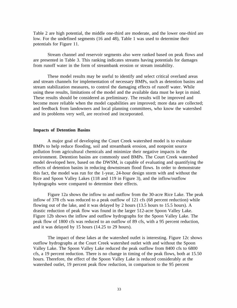
Table 2 are high potential, the middle one-third are moderate, and the lower one-third arelow. For the undefined segments (16 and 48), Table 1 was used to determine theirpotentials for Figure 11.

Stream channel and reservoir segments also were ranked based on peak flows andare presented in Table 3. This ranking indicates streams having potentials for damagesfrom runoff water in the form of streambank erosion or stream instability.

These model results may be useful to identify and select critical overland areasand stream channels for implementation of necessary BMPs, such as detention basins andstream stabilization measures, to control the damaging effects of runoff water. Whileusing these results, limitations of the model and the available data must be kept in mind.These results should be considered as preliminary. The results will be improved andbecome more reliable when the model capabilities are improved; more data are collected;and feedback from landowners and local planning committees, who know the watershedand its problems very well, are received and incorporated.

Impacts of Detention Basins

A major goal of developing the Court Creek watershed model is to evaluateBMPs to help reduce flooding, soil and streambank erosion, and nonpoint sourcepollution from agricultural chemicals and minimize their negative impacts in theenvironment. Detention basins are commonly used BMPs. The Court Creek watershedmodel developed here, based on the DWSM, is capable of evaluating and quantifying theeffects of detention basins in reducing downstream flood flows. In order to demonstratethis fact, the model was run for the 1-year, 24-hour design storm with and without theRice and Spoon Valley Lakes (118 and 119 in Figure 3), and the inflow/outflowhydrographs were compared to determine their effects.

Figure 12a shows the inflow to and outflow from the 30-acre Rice Lake. The peakinflow of 378 cfs was reduced to a peak outflow of 121 cfs (68 percent reduction) whileflowing out of the lake, and it was delayed by 2 hours (13.5 hours to 15.5 hours). Adrastic reduction of peak flow was found in the larger 512-acre Spoon Valley Lake.Figure 12b shows the inflow and outflow hydrographs for the Spoon Valley Lake. Thepeak flow of 1800 cfs was reduced to an outflow of 89 cfs, with a 95 percent reduction,and it was delayed by 15 hours (14.25 to 29 hours).

The impact of these lakes at the watershed outlet is interesting. Figure 12c showsoutflow hydrographs at the Court Creek watershed outlet with and without the SpoonValley Lake. The Spoon Valley Lake reduced the peak outflow from 8400 cfs to 6800cfs, a 19 percent reduction. There is no change in timing of the peak flows, both at 15.50hours. Therefore, the effect of the Spoon Valley Lake is reduced considerably at thewatershed outlet, 19 percent peak flow reduction, in comparison to the 95 percent

33

34

Table 3. Ranking of Stream and Reservoir Segments of Court Creek Watershed Based on Peak Flows in Descending Order Resulting from Design Storms

1-year, 24-hour

2-year, 24-hour

2-year, 6-hour


# Unit-Width

peak flow (cfs/ft)

Overland #


(cfs/ft)

Overland #


(cfs/ft)

Overland #


(cfs/ft)

1 117 6802 117 12823 117 7291 117 17983 2 107 6544 107 12352 107 6951 107 17097 3 105 6300 105 12064 105 6464 105 15932 4 92 3654 92 6922 92 3492 92 8194 5 91 3611 91 6634 91 3215 91 7881 6 104 2767 104 5533 104 3051 104 7876 7 85 1985 85 3760 113 1853 100 4612 8 113 1798 113 3374 100 1784 113 4437 9 100 1670 100 3226 85 1754 85 4218

10 81 1340 98 2632 98 1438 98 3680 11 98 1307 81 2514 97 1211 97 3088 12 90 1195 111 2272 111 1095 111 2669 13 111 1177 90 2230 81 1054 90 2635 14 97 1085 97 2204 90 1042 81 2621 15 110 942 110 1783 103 889 103 2358 16 103 880 103 1739 110 826 110 2049 17 102 796 102 1571 102 760 102 2014 18 84 789 84 1527 95 733 95 1792 19 116 727 88 1504 84 699 84 1734 20 88 717 116 1290 116 607 88 1520 21 95 662 106 1273 94 525 116 1474 22 106 589 95 1233 88 516 106 1346 23 80 576 96 1082 106 506 94 1263 24 112 574 112 1036 112 487 96 1227 25 115 564 115 1023 96 458 112 1150 26 79 544 79 1011 115 408 115 1103 27 96 539 80 985 79 400 79 1066 28 94 491 94 907 80 382 80 946 29 89 427 101 890 89 371 101 922 30 83 426 83 829 83 364 89 919 31 87 415 109 809 109 359 83 917 32 109 413 89 801 101 325 109 907 33 101 403 87 769 99 321 99 817 34 93 378 93 739 93 303 93 801 35 86 356 99 708 82 284 87 776 36 99 342 86 696 86 278 82 708 37 82 334 82 651 87 270 86 686 38 108 287 108 632 108 225 108 590 39 118 121 114 235 118 138 118 360 40 114 118 118 204 114 126 114 304 41 119 88 119 161 119 78 119 214

Figure 12. Comparisons of water discharges in Court Creek watershed resulting froma l-year, 24-hour rainfall in western Illinois and Soil Conservation Service

rainfall distribution showing impact of lakes: (a) inflows to and outflows fromRice Lake, (b) inflows to and outflows from Spoon Valley Lake, and

(c) watershed outflows with and without Spoon Valley Lake

35

reduction immediately downstream of the lake. Impact of the smaller (30-acre) Rice Lakeon the Court Creek watershed outlet, located nearly 14 miles downstream of the lake, isexpected to be negligible.

Effect of Different Watershed Subdivisions

The model runs were made based on division of the Court Creek watershed into78 overland, 39 channel, and 2 reservoir segments (Figure 3). This division helps ininvestigating runoff characteristics in each of the segments and discerns one from theother based on runoff volume and peak flow or unit-width peak flow. If a project requiresfiner resolution, the watershed could be divided into more overland and channel segmentswith smaller areas and lengths, which will require more data processing. However, if theproject does not require as many spatially distributed runoff characteristics, only theoutflows from the watershed and each of the tributaries, it would be efficient to usecoarser division with less overland and channel segments and minimize time and effort indata processing. The question is, how accurate would the model results be? To answerthis question, a coarser division of the Court Creek watershed (Figure 13) is used to runthe DWSM-hydrology. In this division, the watershed was divided into 24 overland (1-24), 12 channel (25-36), and one reservoir (37) segments. Model parameters for thesecoarse segments were derived by averaging parameters of the fine segments (Figure 3)within each of the coarse segments.

The model was run for the April 1, 1983, storm using both subdivisions,respective parameters, and average rainfall intensities derived from rainfall records overthe 12 raingage stations discussed earlier. Predicted outflow hydrographs from both thecoarse and fine divisions are shown in Figure 14 along with the observed outflows andaverage rainfall intensities used in the model runs. Hydrographs from both thesubdivisions are almost the same (Figure 14). Such a match is due to the consistencies ofthe parameters. Parameters of the coarse divisions are averages of the respective finedivisions, and the dynamic routing scheme of the model preserving the dynamicbehaviors of the water flow irrespective of the segment size and length. Therefore, finerdivisions do not necessarily add accuracy to the outflows of larger drainage areas.However, finer divisions allow investigations of spatial distribution of runoffcharacteristics (volume and peak flow) and distinguish these characteristics amongsmaller areas within the watershed. Such results are important to identify problem areas,prioritize them, and find solutions.

36

Figure 13. Coarse model divisions of the Court Creek watershed

37

Figure 14. Comparisons of predicted and observed outflows from the Court Creekwatershed for the April 1, 1983, storm showing effect

of fine and coarse divisions of the watershed

38

Conclusions

A hydrologic model of the Court Creek watershed was developed using thehydrologic component of the DWSM to simulate storm water rainfall-runoff on overlandareas and propagation of flood waves through the overland-stream-reservoir network ofthe watershed. A new routine was introduced into the model to allow simulation ofspatially distributed rainfall events, which is especially useful for moving storms andlocalized thunderstorms. The model was calibrated and verified using three rainfall-runoff events monitored by the ISWS. The calibration and verification produced mixedresults.

The Court Creek watershed is large and has a tile drainage system; this may causea significant amount of subsurface and tile flow to the resultant hydrographs at themonitoring stations. Intense storms cause over bank channel flows and change thedynamics of flood propagation and flows through the monitoring stations. In addition,backwater from the Spoon River, where Court Creek empties, may have an impact on theCourt Creek flows measured at the watershed outlet. The model’s inability to simulatesubsurface, tile, over bank channel flow, and backwater effects are some of the reasonsfor discrepancies in the calibration and verification runs.

Model results depend on accuracy of the input data derived from measurements ofthe physical characteristics of the watershed and monitored hydrological andmeteorological data. Data used in this modeling study were based on limited datameasured and monitored nearly two decades ago for different objectives, not necessarilyfor modeling; therefore, approximations were made in many of the model inputs. Morestream cross-sectional measurements, up-to-date land-use information, dam operationrecords of the two major lakes, and more flow monitoring in the upstream sections of thestreams would improve calibration and verification of the model as well as accuratelyrepresent the watershed.

In spite of its mixed performance, the model demonstrated that it was able torepresent the watershed in simulating its major hydrologic processes and generatinghydrographs that have similar characteristics as the observed hydrographs at themonitoring stations, with limitations on intensities of the storms. Therefore, in this firstattempt of modeling the dynamic behaviors of hydrologic processes in the Court Creekwatershed, the model performance is promising considering the size of the watershed,complexities of the processes being simulated, limitations of available data for the modelinputs, and limitations of the model. This model provides an inexpensive tool to conductpreliminary investigations of the watershed, understand the major hydrologic processesand their dynamic interactions within the watershed, and help solve some of theassociated problems using alternative land use and BMPs, evaluated throughincorporating these into the model inputs.

The model was used to compare model predictions of water discharges based onspatially distributed rainfall inputs and average rainfall input. No differences were foundbecause of a fairly uniform rainfall pattern for the monitored storm simulated. However,

39

the routine will be useful for simulating moving storms and localized thunderstorms. Atest was made to examine effects of different subdivisions. No differences in modelpredictions were found because of the dynamic routing schemes in the model for whichdynamic behaviors were preserved irrespective of the size and length of the segments.Although finer subdivision does not add accuracy to the outflows, it allows investigationsof spatially distributed runoff characteristics and distinguishes these among smaller areasto help prioritize the areas for proper attention.

The calibrated and verified model was used to simulate four synthetic (design)storms to analyze and understand the major dynamic processes in the watershed. Detailedsummaries of results from these model runs are presented. These summary results wereused to rank overland segments based on unit-width peak flows (indicating potential flowstrengths that may damage the landscape) and runoff volumes (indicating potential flood-causing runoff amounts). Stream channel and reservoir segments also were ranked basedon peak flows (indicating potentials for damages to the streams). Maps were generated toshow runoff potentials of overland areas. These results may be useful to identify,prioritize, and select critical overland areas and stream channels for the implementationof necessary BMPs to control damaging effects of runoff water.

The model also was used to evaluate and quantify effects of Rice Lake and SpoonValley Lake, in reducing downstream flood flows and to demonstrate the model’s abilityto evaluate detention basins. The model was run for one of the design storms with andwithout the lakes. The results showed significant reduction (68-95 percent) of peak flowsand delayed their occurrence (up to 15 hours) immediately downstream. The effects werereduced further downstream.

Limitations of the model and the available data must be kept in mind. Theseresults should be considered preliminary. As the model capabilities are improved, moredata are collected, and feedback from the landowner and local planning committees arereceived and incorporated, the results will be improved and become more reliable.Partnership with the Court Creek Watershed Planning Committee, which knows thecharacteristics, problems, and behaviors of the watershed on a daily basis, is extremelyimportant to reflect on the assumptions in model formulations and data preparation.

Efforts are currently under way at the ISWS to add subsurface and tile flowroutines to the DWSM. It is recommended that stream cross-sectional measurements bemade at representative sections of all the major streams in the Court Creek watershed.Stream flow monitoring needs to be continued or established at least at the outlets ofmajor tributaries, including Middle Creek, North Creek, Sugar Creek, and upper CourtCreek upstream of its confluence with the Middle Creek. Monitoring definitely needs tobe continued on Court Creek at the watershed outlet. The last station needs to be far awayfrom the influence of backwater from the Spoon River. It is recommended for continuousrainfall records that a minimum of four raingage stations be spaced equally in thisapproximately square-sized watershed. Approximate locations of these raingages couldbe upstream of North Creek, upstream of Sugar Creek, upstream of Court Creek, anddownstream of Court Creek.

40

References

Ashraf, M.S., and D.K. Borah. 1992. Modeling Pollutant Transport in Runoff andSediment. Transactions of the ASAE 35(6):1789-1797.

Austen, D.J., and A.M. Hogan. 1999a. Pilot Watershed Program Retreat, January 7,1999, Holiday Inn, Urbana, IL. Summary and personal communication, February1, 1999, Illinois Department of Natural Resources-Watershed ManagementSection, Springfield, IL.

Austen, D.J., and A.M. Hogan. 1999b. Pilot Watershed Program Workshop, March 5,1999, Northfield Center, Springfield IL. Proceedings and personalcommunication, March 18, 1999, Illinois Department of Natural Resources-Watershed Management Section, Springfield, IL.

Borah, D.K. 1989a. Runoff Simulation Model for Small Watersheds. Transactions of theASAE 3 2(3):881-886.

Borah, D.K. 1989b. Sediment Discharge Model for Small Watersheds. Transactions ofthe ASAE 32(3):874-880.

Borah, D.K. 1995. Storm Water Management and Flood Forecasting Using WatershedModel RUNOFF. Proceedings of the Water Resources Engineering Conference,August 14-18, 1995, San Antonio, TX, ASCE, pp. 1615-1619.

Borah, D.K., C.V. Alonso, and S.N. Prasad. 1981. Stream Channel Stability, Appendix I.Single Event Numerical Model for Routing Water and Sediment on SmallCatchments. USDA Sedimentation Laboratory, Oxford, MS.

Borah, D.K., M. Bera, S. Shaw, and L. Keefer. 1999a. Dynamic Modeling andMonitoring of Water, Sediment, Nutrients, and Pesticides in AgriculturalWatersheds during Storm Events. Illinois State Water Survey Contract Report655.

Borah, D.K., M. Bera, S. Shaw, L. Keefer, and M. Demissie. 1999b. Dynamic Modelingof Sediment, Nutrient, and Pesticide Transport in Agricultural Watersheds duringSevere Storm Events. Proceedings, Ninth Annual Conference, IllinoisGroundwater Consortium, April 1, 1999, Carbondale, IL, pp. 24-38.

Borah, D.K., M. Demissie, L. Keefer, M. Bera, and S. Shaw. 1998. Dynamic Modeling ofSediment, Nutrient, and Pesticide Transport in Agricultural Watersheds duringSevere Storm Events. Proceedings, Eighth Annual Conference, IllinoisGroundwater Consortium, April 1-2, 1998, Makanda, IL, pp. 128-150.

41

Borah, D.K., S.N. Prasad, and C.V. Alonso. 1980. Kinematic Wave RoutingIncorporating Shock Fitting. Water Resources Research 16(3):529-541.

Chow, V.T. 1959. Open-Channel Hydraulics. McGraw-Hill Book Company, New York.

Demissie, M., L. Keefer, D. Borah, V. Knapp, S. Shaw, K, Nichols, and D. Mayer.1996. Watershed Monitoring and Land Use Evaluation for the Lake DecaturWatershed. Illinois State Water Survey Miscellaneous Publication 169.

Demissie, M., L. Keefer, and R. Xia. 1992. Erosion and Sedimentation in the IllinoisRiver Basin. ILENR/RE-WR-92/04. Illinois Department of Energy and NaturalResources, Springfield, IL.

Demissie, M., T. W. Soong, and N.G. Bhowmik. 1988. Hydraulic Investigation for theConstruction of Artificial Islands in Peoria Lake. ILENR/RE-WR-88/15 andIllinois State Water Survey Contract Report 447. Illinois Department of Energyand Natural Resources, Springfield, IL.

Department of the Army. 1978. Illinois River Basin: ILNONAME Dam 405, SpoonLake, Knox County, Illinois, Inventory Number 00422: Inspection Report,National Dam Safety Program. Department of the Army, Chicago District, U.S.Army Corps of Engineers, Chicago, IL.

Department of the Army. 1979. Illinois River Basin: Lake Rice Dam, Knox County,Illinois, Inventory Number 00421: Inspection Report, National Dam SafetyProgram. Department of the Army, Chicago District, U.S. Army Corps ofEngineers, Chicago, IL.

Fitzpatrick, W.P., W.C. Bogner, and N.G. Bhowmik. 1985. Sedimentation Investigationof Lake Springfield, Springfield, Illinois. Illinois State Water Survey ContractReport 363.

Fitzpatrick, W.P., W.C. Bogner, and N.G. Bhowmik. 1987. Sedimentation andHydrologic Processes in Lake Decatur and Its Watershed. Illinois State WaterSurvey Report of Investigation 107.

Goolsby, D.A., W.A. Battaglin, G.B. Lawrence, R.S. Artz, B.T. Aulenbach, R.P. Hooper,D.R. Keeney, and G.J. Stensland. 1999. Flux and Sources of Nutrients in theMississippi-Atchafalaya River Basin. Task Group 3 Report, Gulf of MexicoHypoxia Assessment. White House Committee on Environment and NaturalResources, Washington, DC.

Huff, F.A., and J.R. Angel. 1989. Frequency Distributions and HydroclimaticCharacteristics of Heavy Rainstorms in Illinois. Illinois State Water SurveyBulletin 70.

42

Illinois Department of Agriculture, Natural Resources Conservation Service, Associationof Illinois Soil and Water Conservation Districts, Farm Service Agency, IllinoisEnvironmental Protection Agency, and Illinois Department of Natural Resources(D.J. Austen, IDNR, coordinator). 1998. The Pilot Watershed Program:Watershed Management, Monitoring and Assessment. IDNR-WatershedManagement Section, Springfield, IL, July 2, 1998.

Keefer, L., M. Demissie, D. Mayer, K. Nichols, and S. Shaw. 1996. WatershedMonitoring and Land Use Evaluation for the Vermilion River Watershed. IllinoisState Water Survey Miscellaneous Publication 176.

Kirpich, P.Z. 1940. Time of concentration of small agricultural watersheds. CivilEngineering 10(6):362.

Lighthill, M.J., and C.B. Whitham. 1955. On Kinematic Waves, 1, Flood Movement inLong Rivers. Proceedings of the Royal Society, London, Ser. A(229):281-316.

Mitchell, J.K., A.S. Felsot, and M.C. Hirschi. 1994. Agricultural practices for waterquality improvement. Proceedings, Fourth Annual Conference, IllinoisGroundwater Consortium, March 23-24, 1994, Makanda, IL, pp. 13-24.

Roseboom, D., R.L. Evans, J. Erickson, and L.G. Brooks. 1982a. An Inventory of CourtCreek Watershed Characteristics that May Relate to Water Quality in theWatershed. Illinois State Water Survey Contract Report 322.

Roseboom, D., R.L. Evans, J. Erickson, and L.G. Brooks. 1982b. Appendices for anInventory of Court Creek Watershed Characteristics that May Relate to WaterQuality in the Watershed. Illinois State Water Survey Contract Report 322A.

Roseboom, D., R.L. Evans, J. Erickson, L.G. Brooks, and D. Shackleford. 1986. TheInfluences of Land Uses and Stream Modifications on Water Quality in theStreams of the Court Creek Watershed. ILENR/RE-WR-86/16, IllinoisDepartment of Energy and Natural Resources, Springfield, IL.

Roseboom, D., T. Hill, J. Rodsater, and A. Felsot. 1990. Stream Yields from AgriculturalChemicals and Feedlot Runoff from an Illinois Watershed. ILENR/RE-WR-90/11,Illinois Department of Energy and Natural Resources, Springfield, IL.

Simons, D.B., R.M. Li, and M.A. Stevens. 1975. Development of Models for PredictingWater and Sediment Routing and Yield from Storms on Small Watersheds.Colorado State University, Fort Collins, CO.

Smith, R.E., and J.Y. Parlange. 1978. A Parameter-efficient Hydrologic InfiltrationModel. Water Resources Research 14(3):533-538.

Soil Conservation Service. 1972. Hydrology. Section 4. In National EngineeringHandbook. SCS, Washington, DC.

43

Soil Conservation Service. 1986. Urban Hydrology for Small Watersheds. TR 55. NTIS,U.S. Department of Commerce, Springfield, VA.

Thiessen, A.H. 1911. Precipitation Averages for Large Areas. Monthly Weather Review39:1082-1084.

Thomas, G. 1998. Enhancing the River. Outdoor Illinois VI(12):2-5.

44

Appendix A.

Hydrology FormulationsUsed in the Dynamic Watershed Simulation Model

45

Rainfall Excess by SCS Runoff Curve Number

The Soil Conservation Service or SCS (1972) runoff curve number method is thesimpler of the two alternative methods used to compute rainfall excess. In this method,estimation of only one parameter, the curve number, for each overland is required.Rainfall excess is computed using the following relations:

(1)

(2)

in which, Qr = direct runoff or rainfall excess (millimeters or mm), P = accumulatedrainfall (mm), and CN = curve number representing runoff potential of a surface (values2-100). Curve number for each overland is estimated based on its soil type, land use,management practices, and antecedent moisture conditions. Accumulated rainfall excessat each breakpoint time interval is computed using these two equations, estimated CN,and the accumulated rainfall at the breakpoint. Increments of rainfall excess during thebreakpoint time intervals are computed by subtracting each accumulated rainfall excessfrom its successive value. Rainfall intensities are computed by dividing the rainfallexcess increments by the corresponding time intervals.

Water Routing through Overland and Channel

The water routing algorithm for both overland and channel flow elements is basedon the kinematic wave approximations (Lighthill and Whitham, 1955) of the Saint-Venant or shallow water wave equations governing unsteady free surface flow. Thegoverning equations are:

(3)

(4)

in which A = flow cross-sectional area, Q = flow rate of water discharge, q = rate oflateral inflow per unit length, t = time, x = downslope position, = kinematic waveparameter, and m = kinematic wave exponent. These equations were written for achannel, and Figure 5 shows the physical interpretations of A, Q, and q. These equationsalso are used for overlands simply by substituting A, Q, and q with flow depth, rate ofwater discharge per unit width, and rate of rainfall excess, respectively. This substitutionis possible because of routing over a unit width of overland as shown in Figure 5 anddiscussed earlier. The kinematic wave parameter and the exponent m are assumed

46

independent of time and piecewise uniform in space (constant within each flow element),and are expressed as:

(5)

(6)

(7)

in which S = longitudinal bed slope of the flow element, n = Manning’s roughnesscoefficient, P = wetted perimeter of the flow element, and a and b = coefficient andexponent, respectively, in wetted perimeter versus flow area relation. For the unit widthof overland, a = 1.0 and b = 0.0. For a channel, a and b are estimated from cross-sectionalmeasurements. The lateral inflow q is assumed piecewise uniform in space and piecewiseconstant in time (constant over a time interval).

Equations 3 and 4 were solved analytically by the method of characteristics, andthe solutions were expressed in the following discretized form (Borah et al., 1980):

(8)

(9)

in which i = subscript representing a discrete point along the x-axis, j = subscriptrepresenting a discrete point along the t-axis, t j = time increment, and x i = spaceincrement, as shown in Figure Al. Figure Al illustrates the water-routing algorithm. Aconstant computational time interval is chosen. The initial flow condition is assumeduniform within the flow elements. Routing is carried out by tracing characteristics andshock paths, starting with the characteristic C0, in the x-t domain. A characteristic istraced starting from the t-axis (x=0) and continued until it intersects the downstream endof the flow element by using the above analytical solution (Equations 8 and 9) andEquation 4. Equation 8 is used to compute A i,j and Equation 4 to compute Qi,j. Equation 9is used to solve for x i which is added to x i-1 to compute a new coordinate (xi ,tj) of thecharacteristic. When there is no lateral inflow (qj = 0), the flow values A and Q remainunchanged along the characteristic, and the space increment is computed as

Because the initial flow condition is assumed uniform, all the characteristicsemanating from the x-axis (t=0) are parallel to C0 and the outflow conditions at times t ,1

t2, t3 , . . . are equal to those computed at the points 1, 2, 3, . . . on C0 (Figure A1). Afterthe initial characteristic C0, the characteristics are traced one from each time intervalemanating from the mid points. Before tracing a characteristic, it is necessary to check ashock-forming condition in which two characteristics meet and the solution fails. Thecondition is:

47

Figure A1. Tracing characteristics and shock paths in kinematic wave routing(after Borah et al., 1980)

48

(10)

If this condition is satisfied, a shock wave (discontinuous water surface or abruptflow depth) is introduced at time tj-1. The shock wave is a discontinuity in which theinitial flow values ahead and behind the shock are A0,j-1 =A0,j-1 and A0,j-1 =A0 , j ,

a b

respectively. The superscripts a and b indicate conditions ahead and behind the shock.The shock path is traced by updating the flow values ahead and behind the shock at theend of each time interval using Equations 8 and 4, and computing the correspondingspace increment using the following expression given by Borah et al. (1980):

(11)

Similar to the characteristics, the procedure of tracing shock path continues untilthe shock intersects the downstream boundary. A single outflow value at the arriving timeinterval is computed by averaging the flow depths or flow areas ahead and behind theshock and converting this to flow using Equation 4. When qj=0, the flow values aheadand behind the shock remain unchanged and the space increment is computed as

Introduction of the shock wave and routing it with the above procedure is calledthe “approximate shock-fitting solution” (Borah et al., 1980). Equations 4, 8, and 9constitute the analytical solution, and Equations 4, 8, and 11 constitute the approximateshock-fitting solution.

The discharges existing on all the characteristics and shock paths at the time ofarrival at the downstream boundary define an outflow distribution. Flow values atintermediate time intervals are computed by linear interpolation. Flow values areaveraged when characteristics and/or shock paths arrive downstream during the sametime interval.

Advantages of this water routing scheme, based on the analytical and approximateshock-fitting solutions of the kinematic wave equations over finite difference numericalsolutions, were demonstrated in Borah et al. (1980).

Water Routing through a Reservoir

Water routing through a reservoir is performed using the storage-indicationmethod (Soil Conservation Service, 1972). The method assumes a level water surfacewithin the reservoir, invariable storage-discharge relation, and steady-state flow duringsmall time intervals. The method is based on the continuity equation, and may beexpressed in the following discretized form:

49

(12)

in which S = reservoir storage, O = outflow rate, I = inflow rate, t = time, and t = timeinterval. Initially, the depth of water (or elevation of the water surface) in the reservoirand the outflow from the reservoir are known. The inflow hydrograph is known orestimated. Therefore, the terms in the right-hand side of Equation 12 also are known. Theoutflows, and thus the outflow hydrograph, are computed by repeatedly using Equation12 and the storage-discharge relation for the reservoir.

50

Appendix B.

Model Results for Design Storms

51

Table B1. Predicted Runoff Volumes and Peak Flows in Overland Segments of Court Creek WatershedResulting from the 1-year, 24-hour Storm in Western Illinois with SCS Rainfall Distribution

Overland#

Overlandarea

(acres)

Overlandarea(mi2)

Curvenumber

Rainfall(in)

Rainfallexcess

(in)

Runoffvolume(ac-ft)

Unit-Widthpeak flow

(cfs/ft)

Width Integratedpeak flow

(cfs)

1 1087 1.7 76 2.79 0.88 79 0.021 3742 613 1.0 76 2.79 0.88 45 0.017 3033 663 1.1 76 2.79 0.88 48 0.022 3754 883 1.4 76 2.79 0.88 64 0.019 3225 922 1.5 76 2.79 0.88 67 0.018 2796 436 0.7 76 2.79 0.88 32 0.024 3767 559 0.9 76 2.79 0.88 41 0.014 1678 689 1.1 76 2.79 0.88 50 0.015 1819 632 1.0 76 2.79 0.88 46 0.023 60

10 211 0.3 76 2.79 0.88 15 0.022 5911 1176 1.9 76 2.79 0.88 86 0.019 26212 547 0.9 76 2.79 0.88 40 0.018 24413 125 0.2 76 2.79 0.88 9 0.018 7314 177 0.3 76 2.79 0.88 13 0.019 7715 601 1.0 76 2.79 0.88 44 0.016 18116 564 0.9 76 2.79 0.88 41 0.016 18617 429 0.7 76 2.79 0.88 31 0.020 20218 578 0.9 76 2.79 0.88 42 0.025 25219 101 0.2 76 2.79 0.88 7 0.018 6720 42 0.1 76 2.79 0.88 3 0.013 4621 1077 1.7 76 2.79 0.88 79 0.016 27822 843 1.3 76 2.79 0.88 62 0.015 26123 904 1.4 76 2.79 0.88 66 0.023 29924 443 0.7 76 2.79 0.88 32 0.019 24425 1385 2.2 78 2.79 0.98 113 0.029 26326 956 1.5 78 2.79 0.98 78 0.023 20927 1053 1.7 78 2.79 0.98 86 0.022 39128 819 1.3 78 2.79 0.98 67 0.022 39829 980 1.6 75 2.79 0.83 67 0.013 20330 703 1.1 75 2.79 0.83 48 0.018 28331 1519 2.4 75 2.79 0.83 105 0.021 20432 1281 2.0 75 2.79 0.83 88 0.026 24633 1224 2.0 75 2.79 0.83 84 0.018 16634 174 0.3 75 2.79 0.83 12 0.015 13635 1181 1.9 75 2.79 0.83 81 0.024 38236 1409 2.3 75 2.79 0.83 97 0.017 26737 1102 1.8 75 2.79 0.83 76 0.026 9838 285 0.5 75 2.79 0.83 20 0.017 6639 1466 2.3 75 2.79 0.83 101 0.021 21840 137 0.2 75 2.79 0.83 9 0.014 14641 406 0.6 75 2.79 0.83 28 0.011 16442 1314 2.1 75 2.79 0.83 90 0.019 273

52

Table B1. (Concluded)

Overland#

Overlandarea

(acres)

Overlandarea(mi2)

Curvenumber

Rainfall(in)

Rainfallexcess

(in)

Runoffvolume(ac-ft)

Unit-Widthpeak flow

(cfs/ft)


(cfs)

43 232 0.4 75 2.79 0.83 16 0.014 9944 801 1.3 75 2.79 0.83 55 0.023 16345 895 1.4 73 2.79 0.73 55 0.019 32146 1041 1.7 73 2.79 0.73 63 0.012 21047 2241 3.6 73 2.79 0.73 137 0.015 37748 675 1.1 73 2.79 0.73 41 0.011 27849 824 1.3 73 2.79 0.73 50 0.012 18550 413 0.7 73 2.79 0.73 25 0.013 19551 193 0.3 77 2.79 0.93 15 0.024 19552 2472 4.0 77 2.79 0.93 191 0.038 30553 787 1.3 76 2.79 0.88 57 0.028 23054 175 0.3 76 2.79 0.88 13 0.017 13755 999 1.6 76 2.79 0.88 73 0.019 33456 1367 2.2 76 2.79 0.88 100 0.019 33957 945 1.5 76 2.79 0.88 69 0.028 43858 1394 2.2 76 2.79 0.88 102 0.022 34459 728 1.2 76 2.79 0.88 53 0.017 20860 308 0.5 76 2.79 0.88 22 0.016 20061 901 1.4 76 2.79 0.88 66 0.021 23362 800 1.3 76 2.79 0.88 58 0.020 22463 637 1.0 76 2.79 0.88 47 0.022 15864 1257 2.0 76 2.79 0.88 92 0.021 15165 583 0.9 78 2.79 0.98 48 0.031 28066 824 1.3 76 2.79 0.88 60 0.018 16467 1769 2.8 76 2.79 0.88 129 0.024 34668 752 1.2 78 2.79 0.98 62 0.025 36069 676 1.1 78 2.79 0.98 55 0.027 40870 1068 1.7 78 2.79 0.98 87 0.022 34071 179 0.3 75 2.79 0.83 12 0.014 6472 507 0.8 75 2.79 0.83 35 0.019 8773 886 1.4 75 2.79 0.83 61 0.017 40874 990 1.6 75 2.79 0.83 68 0.014 33475 438 0.7 75 2.79 0.83 30 0.018 11576 56 0.1 75 2.79 0.83 4 0.009 5877 82 0.1 75 2.79 0.83 6 0.009 8678 243 0.4 75 2.79 0.83 17 0.014 129

53

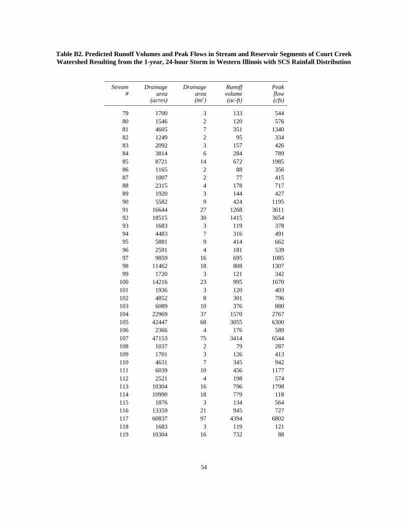
Table B2. Predicted Runoff Volumes and Peak Flows in Stream and Reservoir Segments of Court CreekWatershed Resulting from the 1-year, 24-hour Storm in Western Illinois with SCS Rainfall Distribution

Stream#

Drainagearea

(acres)

Drainagearea(mi2)

Runoffvolume(ac-ft)

Peakflow(cfs)

79 1700 3 133 54480 1546 2 120 57681 4605 7 351 134082 1249 2 95 33483 2092 3 157 42684 3814 6 284 78985 8721 14 672 198586 1165 2 88 35687 1007 2 77 41588 2315 4 178 71789 1920 3 144 42790 5582 9 424 119591 16644 27 1268 361192 18515 30 1415 365493 1683 3 119 37894 4483 7 316 49195 5881 9 414 66296 2591 4 181 53997 9859 16 695 108598 11462 18 808 130799 1720 3 121 342

100 14216 23 995 1670101 1936 3 120 403102 4852 8 301 796103 6089 10 376 880104 22969 37 1570 2767105 42447 68 3055 6300106 2366 4 176 589107 47153 75 3414 6544108 1037 2 79 287109 1701 3 126 413110 4631 7 345 942111 6039 10 456 1177112 2521 4 198 574113 10304 16 796 1798114 10990 18 779 118115 1876 3 134 564116 13359 21 945 727117 60837 97 4394 6802118 1683 3 119 121119 10304 16 732 88

54

Table B3. Predicted Runoff Volumes and Peak Flows in Overland Segments of Court Creek WatershedResulting from the 2-year, 24-hour Storm in Western Illinois with SCS Rainfall Distribution

Overland#

Overlandarea

(acres)

Overlandarea(mi2)

Curvenumber

Rainfall(in)

Rainfallexcess

(in)

Runoffvolume(ac-ft)

Unit-Widthpeak flow

(cfs/ft)


(cfs)

1 1087 1.7 76 3.45 1.33 120 0.040 7242 613 1.0 76 3.45 1.33 68 0.032 5753 663 1.1 76 3.45 1.33 73 0.041 6974 883 1.4 76 3.45 1.33 98 0.036 6105 922 1.5 76 3.45 1.33 102 0.037 5746 436 0.7 76 3.45 1.33 48 0.041 6357 559 0.9 76 3.45 1.33 62 0.029 3448 689 1.1 76 3.45 1.33 76 0.030 3589 632 1.0 76 3.45 1.33 70 0.042 112

10 211 0.3 76 3.45 1.33 23 0.042 11111 1176 1.9 76 3.45 1.33 130 0.037 51812 547 0.9 76 3.45 1.33 61 0.035 48113 125 0.2 76 3.45 1.33 14 0.035 14214 177 0.3 76 3.45 1.33 20 0.036 14515 601 1.0 76 3.45 1.33 67 0.033 37416 564 0.9 76 3.45 1.33 62 0.032 36417 429 0.7 76 3.45 1.33 48 0.037 38018 578 0.9 76 3.45 1.33 64 0.047 47819 101 0.2 76 3.45 1.33 11 0.039 14120 42 0.1 76 3.45 1.33 5 0.018 6721 1077 1.7 76 3.45 1.33 119 0.032 55122 843 1.3 76 3.45 1.33 93 0.031 53623 904 1.4 76 3.45 1.33 100 0.045 58424 443 0.7 76 3.45 1.33 49 0.035 45225 1385 2.2 78 3.45 1.46 168 0.055 50026 956 1.5 78 3.45 1.46 116 0.043 38627 1053 1.7 78 3.45 1.46 128 0.041 73528 819 1.3 78 3.45 1.46 100 0.043 76229 980 1.6 75 3.45 1.27 103 0.026 40830 703 1.1 75 3.45 1.27 74 0.035 54431 1519 2.4 75 3.45 1.27 160 0.042 40332 1281 2.0 75 3.45 1.27 135 0.050 48133 1224 2.0 75 3.45 1.27 129 0.035 32334 174 0.3 75 3.45 1.27 18 0.027 24435 1181 1.9 75 3.45 1.27 125 0.047 74636 1409 2.3 75 3.45 1.27 149 0.032 51837 1102 1.8 75 3.45 1.27 116 0.048 18338 285 0.5 75 3.45 1.27 30 0.035 13539 1466 2.3 75 3.45 1.27 155 0.041 42440 137 0.2 75 3.45 1.27 14 0.022 22541 406 0.6 75 3.45 1.27 43 0.022 32742 1314 2.1 75 3.45 1.27 139 0.038 550

55


Overland#

Overlandarea

(acres)

Overlandarea(mi2)

Curvenumber

Rainfall(in)

Rainfallexcess

(in)

Runoffvolume(ac-ft)

Unit-Widthpeak flow

(cfs/ft)


(cfs)

43 232 0.4 75 3.45 1.27 24 0.028 19944 801 1.3 75 3.45 1.27 85 0.047 33145 895 1.4 73 3.45 1.15 85 0.039 66546 1041 1.7 73 3.45 1.15 99 0.026 44347 2241 3.6 73 3.45 1.15 214 0.030 74748 675 1.1 73 3.45 1.15 64 0.023 57149 824 1.3 73 3.45 1.15 79 0.025 36950 413 0.7 73 3.45 1.15 39 0.027 41251 193 0.3 77 3.45 1.39 22 0.045 36252 2472 4.0 77 3.45 1.39 287 0.069 56353 787 1.3 76 3.45 1.33 87 0.058 47354 175 0.3 76 3.45 1.33 19 0.033 26555 999 1.6 76 3.45 1.33 111 0.038 67456 1367 2.2 76 3.45 1.33 151 0.039 68857 945 1.5 76 3.45 1.33 105 0.056 87158 1394 2.2 76 3.45 1.33 154 0.045 69859 728 1.2 76 3.45 1.33 81 0.031 39060 308 0.5 76 3.45 1.33 34 0.032 39461 901 1.4 76 3.45 1.33 100 0.042 46362 800 1.3 76 3.45 1.33 89 0.038 41763 637 1.0 76 3.45 1.33 71 0.039 28364 1257 2.0 76 3.45 1.33 139 0.038 28265 583 0.9 78 3.45 1.46 71 0.057 50966 824 1.3 76 3.45 1.33 91 0.035 30967 1769 2.8 76 3.45 1.33 196 0.047 66368 752 1.2 78 3.45 1.46 91 0.046 65469 676 1.1 78 3.45 1.46 82 0.046 71070 1068 1.7 78 3.45 1.46 130 0.045 68371 179 0.3 75 3.45 1.27 19 0.026 12372 507 0.8 75 3.45 1.27 54 0.038 17773 886 1.4 75 3.45 1.27 94 0.033 79274 990 1.6 75 3.45 1.27 104 0.027 64675 438 0.7 75 3.45 1.27 46 0.032 21176 56 0.1 75 3.45 1.27 6 0.013 8777 82 0.1 75 3.45 1.27 9 0.014 13178 243 0.4 75 3.45 1.27 26 0.027 257

56

57

Table B4. Predicted Runoff Volumes and Peak Flows in Stream and Reservoir Segments of Court Creek Watershed Resulting from the 2-year, 24-hour Storm in Western Illinois with SCS Rainfall Distribution

Stream #

Drainage area

(acres)

Drainage area (mi2)

Runoff volume (ac-ft)

Peak flow (cfs)

79 1700 3 197 1011 80 1546 2 183 985 81 4605 7 541 2514 82 1249 2 146 651 83 2092 3 240 829 84 3814 6 443 1527 85 8721 14 1019 3760 86 1165 2 138 696 87 1007 2 123 769 88 2315 4 283 1504 89 1920 3 223 801 90 5582 9 654 2230 91 16644 27 1969 6634 92 18515 30 2189 6922 93 1683 3 185 739 94 4483 7 485 907 95 5881 9 632 1233 96 2591 4 285 1082 97 9859 16 1074 2204 98 11462 18 1254 2632 99 1720 3 191 708

100 14216 23 1544 3226 101 1936 3 195 890 102 4852 8 474 1571 103 6089 10 594 1739 104 22969 37 2459 5533 105 42447 68 4827 12064 106 2366 4 279 1273 107 47153 75 5331 12352 108 1037 2 126 632 109 1701 3 194 809 110 4631 7 526 1783 111 6039 10 689 2272 112 2521 4 300 1036 113 10304 16 1193 3374 114 10990 18 1176 235 115 1876 3 204 1023 116 13359 21 1421 1290 117 60837 97 6741 12823 118 1683 3 185 204 119 10304 16 1102 161

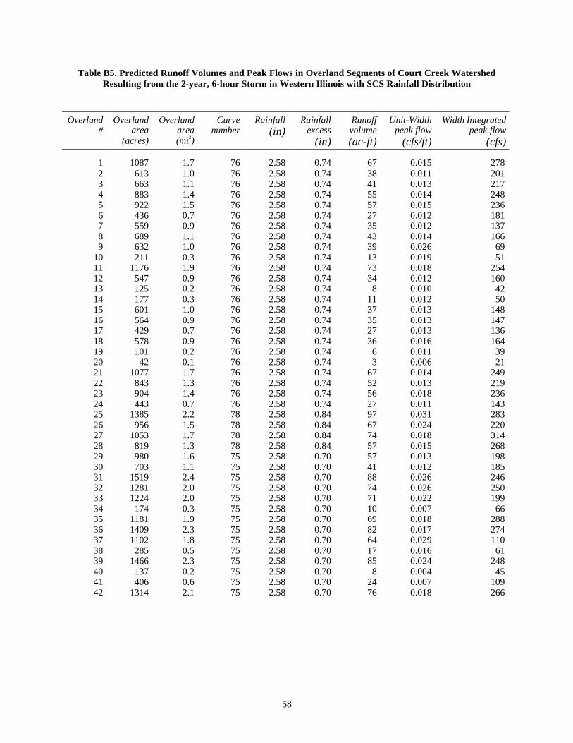
58

Table B5. Predicted Runoff Volumes and Peak Flows in Overland Segments of Court Creek Watershed Resulting from the 2-year, 6-hour Storm in Western Illinois with SCS Rainfall Distribution

Overland #

Overland area

(acres)

Overland area (mi2)

Curve number

Rainfall (in)

Rainfall excess

(in)



(cfs/ft)

Width Integrated peak flow

(cfs)

1 1087 1.7 76 2.58 0.74 67 0.015 278 2 613 1.0 76 2.58 0.74 38 0.011 201 3 663 1.1 76 2.58 0.74 41 0.013 217 4 883 1.4 76 2.58 0.74 55 0.014 248 5 922 1.5 76 2.58 0.74 57 0.015 236 6 436 0.7 76 2.58 0.74 27 0.012 181 7 559 0.9 76 2.58 0.74 35 0.012 137 8 689 1.1 76 2.58 0.74 43 0.014 166 9 632 1.0 76 2.58 0.74 39 0.026 69

10 211 0.3 76 2.58 0.74 13 0.019 51 11 1176 1.9 76 2.58 0.74 73 0.018 254 12 547 0.9 76 2.58 0.74 34 0.012 160 13 125 0.2 76 2.58 0.74 8 0.010 42 14 177 0.3 76 2.58 0.74 11 0.012 50 15 601 1.0 76 2.58 0.74 37 0.013 148 16 564 0.9 76 2.58 0.74 35 0.013 147 17 429 0.7 76 2.58 0.74 27 0.013 136 18 578 0.9 76 2.58 0.74 36 0.016 164 19 101 0.2 76 2.58 0.74 6 0.011 39 20 42 0.1 76 2.58 0.74 3 0.006 21 21 1077 1.7 76 2.58 0.74 67 0.014 249 22 843 1.3 76 2.58 0.74 52 0.013 219 23 904 1.4 76 2.58 0.74 56 0.018 236 24 443 0.7 76 2.58 0.74 27 0.011 143 25 1385 2.2 78 2.58 0.84 97 0.031 283 26 956 1.5 78 2.58 0.84 67 0.024 220 27 1053 1.7 78 2.58 0.84 74 0.018 314 28 819 1.3 78 2.58 0.84 57 0.015 268 29 980 1.6 75 2.58 0.70 57 0.013 198 30 703 1.1 75 2.58 0.70 41 0.012 185 31 1519 2.4 75 2.58 0.70 88 0.026 246 32 1281 2.0 75 2.58 0.70 74 0.026 250 33 1224 2.0 75 2.58 0.70 71 0.022 199 34 174 0.3 75 2.58 0.70 10 0.007 66 35 1181 1.9 75 2.58 0.70 69 0.018 288 36 1409 2.3 75 2.58 0.70 82 0.017 274 37 1102 1.8 75 2.58 0.70 64 0.029 110 38 285 0.5 75 2.58 0.70 17 0.016 61 39 1466 2.3 75 2.58 0.70 85 0.024 248 40 137 0.2 75 2.58 0.70 8 0.004 45 41 406 0.6 75 2.58 0.70 24 0.007 109 42 1314 2.1 75 2.58 0.70 76 0.018 266

59


Overland #

Overland area

(acres)

Overland area (mi2)

Curve number

Rainfall (in)

Rainfall excess

(in)



(cfs/ft)


(cfs)

43 232 0.4 75 2.58 0.70 13 0.009 64 44 801 1.3 75 2.58 0.70 47 0.023 160 45 895 1.4 73 2.58 0.61 46 0.012 208 46 1041 1.7 73 2.58 0.61 53 0.012 195 47 2241 3.6 73 2.58 0.61 114 0.016 386 48 675 1.1 73 2.58 0.61 34 0.007 167 49 824 1.3 73 2.58 0.61 42 0.011 160 50 413 0.7 73 2.58 0.61 21 0.007 111 51 193 0.3 77 2.58 0.79 13 0.011 90 52 2472 4.0 77 2.58 0.79 163 0.048 392 53 787 1.3 76 2.58 0.74 49 0.024 191 54 175 0.3 76 2.58 0.74 11 0.009 70 55 999 1.6 76 2.58 0.74 62 0.014 257 56 1367 2.2 76 2.58 0.74 85 0.017 311 57 945 1.5 76 2.58 0.74 59 0.019 296 58 1394 2.2 76 2.58 0.74 86 0.021 317 59 728 1.2 76 2.58 0.74 45 0.014 175 60 308 0.5 76 2.58 0.74 19 0.010 119 61 901 1.4 76 2.58 0.74 56 0.019 208 62 800 1.3 76 2.58 0.74 50 0.017 191 63 637 1.0 76 2.58 0.74 39 0.020 148 64 1257 2.0 76 2.58 0.74 78 0.026 190 65 583 0.9 78 2.58 0.84 41 0.021 186 66 824 1.3 76 2.58 0.74 51 0.019 172 67 1769 2.8 76 2.58 0.74 110 0.026 366 68 752 1.2 78 2.58 0.84 53 0.017 239 69 676 1.1 78 2.58 0.84 47 0.016 244 70 1068 1.7 78 2.58 0.84 75 0.019 289 71 179 0.3 75 2.58 0.70 10 0.010 46 72 507 0.8 75 2.58 0.70 29 0.020 93 73 886 1.4 75 2.58 0.70 52 0.011 254 74 990 1.6 75 2.58 0.70 58 0.010 246 75 438 0.7 75 2.58 0.70 25 0.015 97 76 56 0.1 75 2.58 0.70 3 0.004 26 77 82 0.1 75 2.58 0.70 5 0.004 39 78 243 0.4 75 2.58 0.70 14 0.008 76

60


Stream # Drainage area

(acres)

Drainage area (mi2)

Runoff volum

(ac-ft)

Peak flow (cfs)

79 1700 3 109 400 80 1546 2 97 382 81 4605 7 290 1054 82 1249 2 79 284 83 2092 3 131 364 84 3814 6 239 699 85 8721 14 558 1754 86 1165 2 73 278 87 1007 2 63 270 88 2315 4 144 516 89 1920 3 120 371 90 5582 9 351 1042 91 16644 27 1063 3215 92 18515 30 1187 3492 93 1683 3 99 303 94 4483 7 264 525 95 5881 9 346 733 96 2591 4 152 458 97 9859 16 583 1211 98 11462 18 672 1438 99 1720 3 101 321

100 14216 23 831 1784 101 1936 3 100 325 102 4852 8 249 760 103 6089 10 313 889 104 22969 37 1311 3051 105 42447 68 2568 6464 106 2366 4 148 506 107 47153 75 2879 6951 108 1037 2 66 225 109 1701 3 107 359 110 4631 7 290 826 111 6039 10 386 1095 112 2521 4 164 487 113 10304 16 674 1853 114 10990 18 665 126 115 1876 3 112 408 116 13359 21 803 607 117 60837 97 3683 7291 118 1683 3 99 138 119 10304 16 626 78

61

Table B7. Predicted Runoff Volumes and Peak Flows in Overland Segments of Court Creek Watershed Resulting from the 10-year, 6-hour Storm in Western Illinois with SCS Rainfall Distribution

Overland #

Overland area

(acres)

Overland area (mi2)

Curve number

Rainfall (in)

Rainfall excess

(in)



(cfs/ft)


(cfs)

1 1087 1.7 76 3.70 1.51 137 0.042 759 2 613 1.0 76 3.70 1.51 77 0.028 509 3 663 1.1 76 3.70 1.51 84 0.034 578 4 883 1.4 76 3.70 1.51 111 0.034 583 5 922 1.5 76 3.70 1.51 116 0.035 547 6 436 0.7 76 3.70 1.51 55 0.025 396 7 559 0.9 76 3.70 1.51 70 0.028 330 8 689 1.1 76 3.70 1.51 87 0.035 418 9 632 1.0 76 3.70 1.51 80 0.077 204

10 211 0.3 76 3.70 1.51 27 0.048 129 11 1176 1.9 76 3.70 1.51 148 0.047 649 12 547 0.9 76 3.70 1.51 69 0.033 464 13 125 0.2 76 3.70 1.51 16 0.027 111 14 177 0.3 76 3.70 1.51 22 0.035 145 15 601 1.0 76 3.70 1.51 76 0.031 356 16 564 0.9 76 3.70 1.51 71 0.033 382 17 429 0.7 76 3.70 1.51 54 0.037 375 18 578 0.9 76 3.70 1.51 73 0.047 475 19 101 0.2 76 3.70 1.51 13 0.028 102 20 42 0.1 76 3.70 1.51 5 0.012 43 21 1077 1.7 76 3.70 1.51 136 0.037 647 22 843 1.3 76 3.70 1.51 106 0.032 564 23 904 1.4 76 3.70 1.51 114 0.047 612 24 443 0.7 76 3.70 1.51 56 0.029 381 25 1385 2.2 78 3.70 1.65 191 0.077 698 26 956 1.5 78 3.70 1.65 132 0.057 513 27 1053 1.7 78 3.70 1.65 145 0.043 773 28 819 1.3 78 3.70 1.65 113 0.042 750 29 980 1.6 75 3.70 1.45 118 0.033 514 30 703 1.1 75 3.70 1.45 85 0.035 547 31 1519 2.4 75 3.70 1.45 183 0.065 626 32 1281 2.0 75 3.70 1.45 154 0.062 593 33 1224 2.0 75 3.70 1.45 147 0.055 506 34 174 0.3 75 3.70 1.45 21 0.017 152 35 1181 1.9 75 3.70 1.45 142 0.051 810 36 1409 2.3 75 3.70 1.45 170 0.041 649 37 1102 1.8 75 3.70 1.45 133 0.090 341 38 285 0.5 75 3.70 1.45 34 0.042 160 39 1466 2.3 75 3.70 1.45 177 0.062 643 40 137 0.2 75 3.70 1.45 16 0.014 143 41 406 0.6 75 3.70 1.45 49 0.022 321 42 1314 2.1 75 3.70 1.45 158 0.047 690

62


Overland #

Overland area

(acres)

Overland area (mi2)

Curve number

Rainfall (in)

Rainfall excess

(in)



(cfs/ft)


(cfs)

43 232 0.4 75 3.70 1.45 28 0.027 189 44 801 1.3 75 3.70 1.45 96 0.059 415 45 895 1.4 73 3.70 1.32 98 0.038 642 46 1041 1.7 73 3.70 1.32 114 0.031 529 47 2241 3.6 73 3.70 1.32 246 0.039 958 48 675 1.1 73 3.70 1.32 74 0.020 493 49 824 1.3 73 3.70 1.32 90 0.027 410 50 413 0.7 73 3.70 1.32 45 0.022 324 51 193 0.3 77 3.70 1.58 25 0.028 231 52 2472 4.0 77 3.70 1.58 326 0.115 937 53 787 1.3 76 3.70 1.51 99 0.057 460 54 175 0.3 76 3.70 1.51 22 0.023 187 55 999 1.6 76 3.70 1.51 126 0.040 704 56 1367 2.2 76 3.70 1.51 172 0.045 806 57 945 1.5 76 3.70 1.51 119 0.053 819 58 1394 2.2 76 3.70 1.51 176 0.053 820 59 728 1.2 76 3.70 1.51 92 0.034 420 60 308 0.5 76 3.70 1.51 39 0.025 311 61 901 1.4 76 3.70 1.51 114 0.049 542 62 800 1.3 76 3.70 1.51 101 0.041 456 63 637 1.0 76 3.70 1.51 80 0.045 332 64 1257 2.0 76 3.70 1.51 158 0.064 467 65 583 0.9 78 3.70 1.65 80 0.058 517 66 824 1.3 76 3.70 1.51 104 0.047 418 67 1769 2.8 76 3.70 1.51 223 0.063 888 68 752 1.2 78 3.70 1.65 103 0.047 666 69 676 1.1 78 3.70 1.65 93 0.040 618 70 1068 1.7 78 3.70 1.65 147 0.043 666 71 179 0.3 75 3.70 1.45 22 0.025 116 72 507 0.8 75 3.70 1.45 61 0.051 240 73 886 1.4 75 3.70 1.45 107 0.030 702 74 990 1.6 75 3.70 1.45 119 0.026 621 75 438 0.7 75 3.70 1.45 53 0.039 257 76 56 0.1 75 3.70 1.45 7 0.008 55 77 82 0.1 75 3.70 1.45 10 0.009 83 78 243 0.4 75 3.70 1.45 29 0.022 207

63


Stream #

Drainage area

(acres)

Drainage area (mi2)


Peak flow (cfs)

79 1700 3 223 1066 80 1546 2 197 946 81 4605 7 583 2621 82 1249 2 160 708 83 2092 3 269 917 84 3814 6 493 1734 85 8721 14 1107 4218 86 1165 2 149 686 87 1007 2 136 776 88 2315 4 309 1520 89 1920 3 246 919 90 5582 9 719 2635 91 16644 27 2166 7881 92 18515 30 2433 8194 93 1683 3 205 801 94 4483 7 546 1263 95 5881 9 721 1792 96 2591 4 321 1227 97 9859 16 1235 3088 98 11462 18 1431 3680 99 1720 3 212 817

100 14216 23 1746 4612 101 1936 3 219 922 102 4852 8 536 2014 103 6089 10 679 2358 104 22969 37 2790 7876 105 42447 68 5449 15932 106 2366 4 310 1346 107 47153 75 5968 17097 108 1037 2 137 590 109 1701 3 215 907 110 4631 7 589 2049 111 6039 10 770 2669 112 2521 4 334 1150 113 10304 16 1338 4437 114 10990 18 1333 304 115 1876 3 227 1103 116 13359 21 1605 1474 117 60837 97 7422 17983 118 1683 3 205 360 119 10304 16 1253 214

Hydrologic Modeling of the Court Creek Watershed calibration and verification runs demonstrated that...

Documents

Transcript of Hydrologic Modeling of the Court Creek Watershed calibration and verification runs demonstrated that...