HYDROGEOLOGIC CHARACTERIZATION AND TEST WELL FEASIBILITY ...

HYDROGEOLOGIC CHARACTERIZATION AND TEST WELL FEASIBILITY ANALYSIS

for SAN LUCAS COUNTY WATER DISTRICT

MONTEREY COUNTY

Prepared for: MONTEREY COUNTY RESOURCE MANAGEMENT AGENCY

REDEVELOPMENT AND HOUSING OFFICE

Prepared by: Pueblo Water Resources, Inc.

Gus Yates, P.G., C.Hg., Consulting Hydrologist Martin Feeney, P.G., C.Hg., Consulting Hydrogeologist

September 2010

September 2010 Project No. 09-0061

09-0061 san lucas hydro characterization and feasibility analysis rpt sept 2010

- i -

Gus Yates, P.G., C.Hg., Consulting HydrologistMartin Feeney, P.G., C.Hg., Consulting Hydrogeologist

TABLE OF CONTENTS

Page

INTRODUCTION .......................................................................................................... 1

FINDINGS..................................................................................................................... 2

Location and Geologic Setting .......................................................................... 2 SLCWD Water System and Historical Production............................................. 3 Groundwater Levels .......................................................................................... 4 Groundwater Quality ......................................................................................... 5 Patterns and Trends in TDS Concentration ...................................................... 5 Patterns and Trends in Ionic Composition ........................................................ 6 Stable Isotope Composition .............................................................................. 8 Land Use and Irrigation..................................................................................... 8

CONCLUSIONS AND RECOMMENDATIONS............................................................. 9

Conclusions Regarding Source of Salinity ........................................................ 9 Options for Improving Water Quality ................................................................. 11 Recommendations ............................................................................................ 12

REFERENCES CITED.................................................................................................. 13

FIGURES

1 Map of the San Lucas Area 2 Surficial Geology of the San Lucas Area 3a Cross Section SW-NE from Springer (2002) 3b Cross Section NW-SE from Springer (2002) 4 Groundwater Production by San Lucas County Water District, 1998-2008 5 Locations of Wells with Water Level Measurement Records 6 Hydrographs of Water Levels in Wells in the San Lucas Area 7 Map of Water Quality Wells and TDS Concentrations 8 Chemographs of Total Dissolved Solids Concentrations in Wells in the San Lucas Area 9 Annual Discharge in the Salinas River near Bradley, Water Years 1950-2009 10 Tri-linear (Piper) Plot of Groundwater Quality in the San Lucas Area 11 Map of Groundwater Quality Composition in the San Lucas Area 12 Box-plots of Total Dissolved Solids Concentration in Water Quality Groups 13 Composition of Groundwater at SLCWD Well #2 and Nearby Water Table Auger Holes 14 Deuterium and O-18 Composition of Water Samples in the San Lucas Area 15a Aerial Photograph of the Floodplain Area near SLCWD Well #2, May 10, 1994 15b Aerial Photograph of the Floodplain Area near SLCWD Well #2, August 30, 2004 15c Aerial Photograph of the Floodplain Area near SLCWD Well #2, August 30, 2006 15d Aerial Photograph of the Floodplain Area near SLCWD Well #2, July 30, 2007 15e Aerial Photograph of the Floodplain Area near SLCWD Well #2, May 25, 2009


C:\DOCUMENTS AND SETTINGS\MICHAEL BURKE\MY DOCUMENTS\PROJECT FILES\SAN LUCAS\09-0061 SAN LUCAS HYDRO CHARACTERIZATION AND FEASIBILITY ANALYSIS RPT SEPT 2010.DOC

- 1 -


INTRODUCTION

San Lucas is a community of approximately 400 residents located near the upper end of the Salinas Valley, between King City and San Ardo. The community water system is supplied by a well (SLCWD Well #2) located in agricultural land about 1.2 miles south of town, on the floodplain of the Salinas river. Water quality in the well met primary drinking water standards from the time it was drilled in 1981 until 2007, when the dissolved solids (TDS) concentration in the well water began rising rapidly. However, iron and particularly manganese have been high ever since the well was drilled, and the water is presently treated at the wellhead to remove those constituents. The objective of the present study is to identify the cause of the increase in TDS and recommend a corresponding corrective strategy. Tracing the source of the salt requires an understanding of the vertical and horizontal distribution of salinity within the groundwater system and the relation of salinity to geologic formations and current processes such as river recharge, groundwater pumping, and irrigation return flow. This memorandum systematically evaluates the following potential causes for the change in salinity SLCWD Well #2:

o A change in the condition of the well itself, such as leaks caused by corrosion that allow poor-quality shallow groundwater to enter the casing

o The abrupt arrival of poor-quality groundwater that has been gradually moving toward the well location for many years.

o A change in regional groundwater levels and gradients that has caused poor-quality groundwater from a nearby part of the basin to enter the capture zone of the well.

o A change in the flow regime of the Salinas River that diminishes the amount of river recharge.

o A change in the amount or quality if groundwater recharge near Well #2 due to a change in overlying land use.

o A change in pumping at nearby irrigation wells that has intercepted the former flow of Salinas River recharge to Well #2.

Data collected for this analysis includes general mineral and stable isotope samples from the Salinas River, a well near SLCWD Well #2, an irrigation well at San Lucas School (SL-33 in Figure 1), and two holes hand-augered to the water table near Well #2. Because historical trends are of central importance, the study relies heavily on data presented in previous studies of groundwater and water supply in the San Lucas area, including EMCON Associates (1986) and especially TRAK Environmental Group (TRAK, 2002). Additional historical data were obtained from files at SLCWD and the Monterey County Environmental Health Division. The EMCON report focused on nitrate contamination of groundwater beneath the town due to the high concentration of septic systems and numerous old domestic wells constructed without seals. That investigation eventually led to the construction of a sewer system and centralized



- 2 -


wastewater treatment plant. The objective of the TRAK study was similar to the objective of the present study: to investigate hydrogeological conditions in the vicinity of San Lucas and determine whether other locations or aquifer intervals could potentially provide improved water quality for the municipal supply. At the time of that study, however, the principal water quality concerns were high iron and manganese; TDS was still lower than the drinking water standard.

FINDINGS

Location and Geologic Setting

San Lucas is located on an old terrace of the Salinas River, on the northeastern edge of the Salinas Valley groundwater basin. Figure 1 shows the location of San Lucas and surrounding features, including SLCWD’s primary supply well (SLCWD-2) and standby well (SLCWD-1) and major irrigation wells in the vicinity. The groundwater basin coincides approximately with the valley floor. The principal basin fill deposits (Paso Robles Formation and younger alluvium) extend laterally to toe of the hillsides adjacent to each side of the basin. Geologically, the basin is a structural trough, or syncline filled with fluvial and alluvial deposits ranging in age from Pliocene to Recent. Figure 2 shows a map of surficial geology in the San Lucas area based largely on work by Tom Dibblee. Previous geologic maps and studies of the basin include Durham (1963) and Dibblee (1971a, b, c and d). Geologic nomenclature differs among those studies, particularly regarding the name of the unit that forms the base of the basin. Durham classified it as an unnamed Pliocene marine formation, parts of which had been included in the Poncho Rico, Santa Margarita and Monterey Formations by previous investigators. Dibblee mapped the unit exposed broadly in the hills northeast of San Lucas as a marine mudstone member of the Poncho Rico Formation. The GIS compilation of geologic mapping completed by Monterey County (Rosenberg, 2001) follows Dibblee’s work, so his nomenclature is used here. The marine origin of the formation results in groundwater that is high in dissolved solids. The Paso Robles Formation comprises the bulk of the basin fill deposits. It pinches out against the underlying Pancho Rico Formation along the northeastern edge of the basin, where stream dissection has left it as a thin cap on hills and ridges. Its maximum thickness near the center of the valley is approximately 1,200 feet (Durham, 1963). The Paso Robles Formation is a heterogeneous mixture of discontinuous layers and lenses of sand, silt, clay and gravel deposited during the Pliocene and Pleistocene ages under continental (nonmarine) conditions. The Paso Robles is overlain by fluvial deposits of varying ages associated with the Salinas River. Along the edges of the valley are older terraces that form flat areas overlooking the current floodplain of the river. The town of San Lucas is situated on one of the terraces. Eolian (sand dune) deposits are present on top of the terraces in several locations between San Lucas



- 3 -


and King City, including a 1,400-acre area immediately adjacent to and extending northwest from San Lucas. Floodplain deposits form flat areas at low elevation adjacent to the river channel, including the 1,300-acre tract of cropland surrounding Well #2. The river flows along a broad, shallow channel containing sand and gravel materials that are actively scoured and redeposited during flood events. The channel, floodplain and terrace deposits have a combined thickness of up to approximately 200 feet near the center of the valley. Figure 3 shows geologic cross sections near San Lucas developed for a previous investigation (TRAK, 2002). The floodplain where Well #2 is located contains a continuous surficial sandy layer 25-40 feet thick. This relatively coarse-textured layer facilitates strong hydraulic coupling between the river and adjacent groundwater system. Although Durham (1963) mapped alluvial deposits near the cross section locations as about 200 feet thick, the transition from alluvium to Paso Robles Formation is not obvious in the TRAK cross sections. All of the floodplain wells for which well logs are available are screened at depths less than 200 feet and are presumably pumping primarily from the alluvial deposits. Toward the edges of the valley, wells of similar depth probably extract water increasingly from the Paso Robles and possibly Poncho Rico Formations. Driller’s logs for four other wells in the floodplain area are available. They were all drilled in 1974 for Las Colinas Vineyards and are referred to as wells #1, #6, #8, and "domestic". All four wells are 90-100 feet deep and have 40 feet of screen. Two of the logs included a 10-foot clay interval; otherwise all of the materials encountered were top soil, sand, gravel and some large rocks. The similarity of geology and well construction among these four wells suggests that they are probably representative of the remaining irrigation wells.

SLCWD Water System and Historical Production

SLCWD operates two wells, both located in the floodplain between the Salinas River and the elevated terrace on which the town is located (see Figure 1). SLCWD Well #1 is nominally a standby well but has not been used in years (William Marcum, personal communication, 6/22/10). It was drilled in November 1980 near a bend in the Lockwood-San Lucas Road, approximately 100 feet east of State Highway 101. The log encountered coarse, sandy materials from 0-20 feet and from 71-160 feet. The intervening interval contained “shale” and “blue clay and sand”. A resistivity log shows the upper contact between coarse and fine materials to be sharp, whereas the lower contact is transitional between 90 and 110 feet below ground surface. The well is screened from 90-140 feet and has a surface seal extending to 80 feet. A pump test in 1991 listed a flow rate of 136 gpm with 10 feet of drawdown. SLCWD Well #2 is the primary supply well for San Lucas. It was drilled in May 1981 near the center of a 1,300-acre floodplain agricultural area 1.2 miles south of San Lucas. Previous studies do not indicate why it was considered necessary to drill a second supply well only 6 months after completing Well #1. The driller’s log for Well #2 reported sandy materials from 0-30 feet and 37-73 feet below ground surface. The intervening 7 feet contained clay. The well is



- 4 -


screened from 35-70 feet and has a surface seal extending to 35 feet. A pump test in 1991 reported a pumping rate of 115 gpm with a drawdown of 2.9 feet. Water from Well #2 is chlorinated at the well site and also treated to remove manganese, which has consistently exceeded the secondary drinking water standard. The water is pumped to a 300,000 gallon storage tank located near town and from there into the distribution system. The tank was installed in 2006, along with new water mains. The municipal wastewater treatment plant, storage ponds and sprayfield disposal areas are located approximately 1 mile east of San Lucas near Highway 198, in an area that is not upgradient of SLCWD Well #2. Figure 4 shows monthly and annual groundwater production by SLCWD during 1998-2008. Annual production has remained fairly stable at an average of 55 acre-feet per year (ac-ft/yr). Groundwater production is greater in summer because of residential landscape irrigation. A curve separation analysis (assuming February water use is 100% indoor use and that indoor use is constant year-round) indicated that 73% of annual groundwater production is used indoors. The large turf area at San Lucas School is irrigated by a separate on-site well (well SL-33 in Figure 1).

Groundwater Levels

Patterns and trends in groundwater levels were explored by compiling and plotting water level data obtained from Monterey County Water Resources Agency (MCWRA). Figure 5 shows the locations of fourteen wells between King City and San Ardo with more than 30 years of data, including measurements within the past 15 years. Figure 6 shows hydrographs of water levels at those wells, which reveal several patterns. First, water levels are remarkably stable because a flow of 200-600 cfs is maintained in the Salinas River throughout the summer of most years by releases from Nacimiento and San Antonio Reservoirs. The typical seasonal fluctuation in groundwater levels is less than 10 feet. Downstream of San Lucas (wells in township 20, with well numbers beginning “20S”) up to 15 feet of drawdown was experienced around 1990, after several years of drought. Water levels in the San Lucas-San Ardo area (township 21) did not even experience this small drought decline. At well 21S/9E-16E01, near SLCWD Well #2, water levels remained within a 4-foot interval throughout 1980-2009. The hydrographs also show that the depth to water near SLCWD #2 is quite shallow, only 8-12 feet below ground surface. This is consistent with two holes hand-augered to the water table near Well #2 in November, 2009. The depth to water in the holes was 7-10 feet below the ground surface, with the shallower water table in the hole closer to the river.



- 5 -


Groundwater Quality

Water quality monitoring is not as systematic as monitoring of groundwater levels. The number of constituents analyzed, the frequency of sampling and the total number of samples collected vary widely from well to well. However, available data are sufficient to characterize historical patterns in TDS concentration and ionic composition of groundwater.

Patterns and Trends in TDS Concentration

Figure 7 shows locations of 34 wells between King City and San Ardo with at least one measurement of total dissolved solids. The wells are labeled with the last part of the state well number, and the symbol colors indicate the most recent measured TDS concentration1. There appears to be a slight correlation between TDS and distance from the river. Wells with low TDS tend to be near the river; wells with high TDS tend to be close to the edge of the valley. The map oversimplifies the TDS distribution on the floodplain where SLCWD Well #1 and Well #2 are located. Irrigation throughout the floodplain is supplied primarily by the five wells on the levee at the southern end of the floodplain (irrigation wells AL-1 thorugh AL-5 in Figure 1). A single measurement of electrical conductivity at an irrigation sprinkler in October 2009 was 700 µS/cm, which corresponds to a TDS concentration of approximately 455 mg/L. The water cannot be traced to a particular well, because water from all of the wells is comingled in storage basins before being pumped into the irrigation distribution system. Given the shallow depths and proximity of the wells to each other, their water qualities are probably similar. The five wells are 600-1,100 feet from the present low-flow channel of the Salinas River (less than 200 feet during high flows) at an outside bend in the river. They appear to function as an infiltration gallery that induces percolation of large amounts of high-quality river water.

Figure 8 shows time series plots of TDS concentration at 24 wells in the San Lucas region that have at least three data points over a period of at least 8 years. The plots reveal historical trends toward increasing TDS in about half of the wells. These wells are located throughout the study area with no obvious geographic pattern. The increasing trend is most apparent during 1988-1994 and could be related to decreased river recharge toward the end of the 1987-1992 drought. Figure 9 shows annual discharge in the Salinas River at the nearest gage upstream of San Lucas (near Bradley) during water years 1951-2009. Flows have been regulated by Nacimiento and San Antonio Reservoirs since 1967, resulting in a typical annual discharge of slightly over 200,000 AFY and much higher discharge in occasional wet years. During the 1987-1992 drought, however, releases averaged only 67% of the long-term median, and were only 3% of the median in 1990. The drought coincided with the onset of TDS increases at many wells and suggests that river recharge usually dilutes ambient groundwater

1 The most recent measurement that did not appear anomalous was selected from TDS time series plots. Only wells with data more recent than 1984 were included. Most of the selected values were from the 1990s.



- 6 -


derived from rainfall/irrigation recharge or inflow from upland areas. Unfortunately, 1994 is toward the end of the period of record for many wells; data for 1995-2009 are much more sparse. It is not clear whether the increasing trends continued at many wells or were reversed by relatively wet conditions in the mid-late 1990s.

TheTDS trends at SLCWD #2 (see plot included in Figure 8) was irregularly upward during 1982-1998, steadily downward during 1999-2004 and very steeply upward during 2007-2010. The start of the recent upward trend coincided with the conversion of cropland on the floodplain from nonirrigated vineyard to irrigated truck crops. In addition to an increase in irrigation pumping, the land was extensively graded during the conversion (Susan Madson, personal communication, August 2009). Historical satellite images documenting the conversion are discussed presented below under "Land Use". The timing of the recent TDS trend strongly suggests that it was caused by the land use conversion. This still leaves two potential mechanisms of water quality degradation. The first is downward percolation of irrigation return flow that is high in TDS due to evaporative concentration during irrigation and crop evapotranspiration. The second is that increased pumping at the irrigation wells altered groundwater flow patterns in the floodplain area such that poor quality groundwater moved into the area surrounding SLCWD Well #2. The quality of groundwater at the water table reflects the quality of recent recharge from rainfall and irrigation return flow. Groundwater TDS at the water table near well SLCWD #2 appears to be slightly higher in general than at the depth of the well screen (24-59 feet below the water table). The water table samples from the two auger holes in November 2009 had TDS concentrations of 1,598 and 1,902 mg/L. The TDS concentration in SLCWD Well #2 was 1,448 mg/L (January 2008) and in a nearby domestic well was 1,660 mg/L (November 2009). Thus, shallow groundwater entering the casing through a corrosion hole near the water table could theoretically cause the observed TDS concentrations in the well, provided the hole was large and the difference in water level across the casing wall was large (both circumstances are fairly unlikely). Thus, the TDS data do not definitively point to one or the other mechanism for irrigation-related increase in TDS in Well #2. However, the ionic composition of well water and shallow groundwater can indicated which of these two mechanisms is more likely.

Patterns and Trends in Ionic Composition

The two most likely potential sources of the high-TDS groundwater in Well #2 are deep percolation of irrigation return flow and migration of poor quality groundwater from the Poncho Rico Formation, which underlies the hills adjacent to the northeastern edge of the Salinas Valley Basin. It was anticipated that the change in TDS would be accompanied by a change in ionic composition, so the proportions of major ions in groundwater from wells at various depths and



- 7 -


locations were compared. The change in composition at SLCWD Well #2 was similarly evaluated. The proportions of the major ions in groundwater samples from the San Lucas region reveals two primary water quality types, with intermediate compositions in many wells reflecting a mixture of those two end members. One end member is water in the Salinas River, which provides sufficient recharge to dominate water quality in wells near the river. The other end member appears to be groundwater in geologic formations that border the northeastern edge of the basin, principally the Poncho Rico Formation. For this discussion, groundwater of that type is referred to as "Poncho Rico" groundwater. The two types are distinguishable on the basis of TDS, ionic composition and stable isotopes. Water in the Salinas River near Bradley has a TDS concentration of 200-500 mg/L, with the higher values occurring during certain low-flow periods and the lower values occurring during high flows and some low-flow periods. When wells were sampled for this project in November 2008, Salinas River water had a TDS concentration of 256 mg/L. The sample collected from the San Lucas School irrigation well (SL-33) in November 2009 is the sample that most closely represents Poncho Rico groundwater. It had a TDS concentration of 1,956 mg/L. Piper plots are the standard method for displaying major-ion compositions of different types of water. Figure 10 is a Piper plot of water from 29 wells in the San Lucas region, plus the Salinas River. The water quality spans a spectrum between Salinas River type water and Poncho Rico type water, with intermediate compositions presumably reflecting mixtures of those two types. Six groups of samples were identified based on the bicarbonate percentage of the anion composition. The bicarbonate-sulfate ratio accounts for most of the variation in composition among the samples. The groups ranged from Salinas river water (group 1: 60-75% bicarbonate) to Poncho Rico groundwater (group 7: 15-25% bicarbonate). The purpose of dividing the continuum of compositions into groups was to allow the groups to be plotted on a map for spatial analysis. The composition of groundwater varies with distance from the river, as would be expected from the hypothesized sources of the two water quality types. Figure 11 shows a map of groundwater quality composition based on the water quality groups. Like the map of groundwater TDS (Figure 7), wells in group 2 (closest to river water composition) tend to be near the river, and wells in group 6 (close to Poncho Rico Formation composition) tend to be far from the river. The correlation of ionic composition and TDS is confirmed in Figure 12, which shows boxplots of TDS concentration for the six water quality groups. TDS concentration increases fairly uniformly from group 2 to group 6, concurrent with the shift from bicarbonate to sulfate anionic composition.



- 8 -


The evolution of ionic composition in Well #2 is displayed in Figure 13, which shows a Piper plot of historical data for Well #2 and for water table samples obtained from the nearby hand-augered holes. The trend in Well #2 water away from the Salinas River water composition and toward the Poncho Rico composition might have started before the land use conversion. However, the most recent sample—collected after TDS began rising rapidly—was clearly closer to the Poncho Rico composition than the Salinas River composition. In contrast, the two water table samples from the auger holes are closer to the Salinas River composition than groundwater currently pumped by well SLCWD #2. This indicates that deep percolation of rainfall and irrigation water has a composition similar to that of the irrigation water but distinct from water in Well #2. This demonstrates that recently recharged groundwater from the water table is not the source of high salinity in Well #2.

Stable Isotope Composition

Stable isotopes of hydrogen and oxygen were measured in six samples collected in the San Lucas area in November 2009. A plot of δ2H versus δ18O is shown in Figure 14. The results further confirm the conceptual model of mixing between Salinas River water and Poncho Rico groundwater, which appear as the two endpoints of the data arrayed on the plot (sites 3 and 6). Groundwater from well SLCWD Well #2 and a domestic well located 100 feet away (sites 1 and 4) had identical isotopic compositions that plotted slightly more than one-third of the way between the Poncho Rico and Salinas River compositions. Water table samples from the two auger holes near Well #2 (points 2 and 5) plotted midway between the Well #2 and Salinas River samples, as expected for an irrigation source similar in composition to Salinas River water. The water table samples are also shifted slightly to the right of the line connecting the other points, consistent with partial evaporation of applied irrigation water.

Land Use and Irrigation

Approximately 900 acres of the 1,300-acre floodplain area surrounding SLCWD Well #2 was converted from non-irrigated, decadent vineyard to irrigated truck crops during 2006-2007. The conversion reportedly involved extensive land grading and importation of topsoil (Susan Madson, personal communication, August 2009). The change in land use is clearly evident in the series of satellite images shown in Figures 15a through 15e. The photographs are from 1994, 2004, 2006, 2007 and 2009. Although direct measurements of agricultural water use on the floodplain are not available, the change in land use was certainly accompanied by a large increase in agricultural pumping. Although the floodplain was presumably irrigated in the 1970s—or the irrigation wells would not have been installed—the vineyards were reportedly not irrigated for a number of years prior to the land use conversion in 2006. The sparse canopy evident in the 1994 through 2006 aerial photographs supports that assertion. Sprinkler irrigation of truck crops in the upper Salinas



- 9 -


Valley typically uses about 3.7 feet of applied water per year1. On 900 acres of cropland, this would amount to approximately 3,300 acre-feet of pumping per year, which is 60 times more groundwater than is pumped by SLCWD Well #2. Most of the agricultural pumping appears to be from the five irrigation wells along the levee at the south end of the floodplain area (wells AL-1 through AL-5 in Figure 1). Two of the five irrigation wells along the dirt road between SLCWD Well #2 and the Salinas River appear to be operational. A third (the one across the road from Well #2) has been converted to domestic use, and its annual production is probably negligible. Groundwater is pumped into the three storage ponds visible in the aerial photographs (Figure 15), and from there into the irrigation distribution system.

CONCLUSIONS AND RECOMMENDATIONS

Conclusions Regarding Source of Salinity

The most likely explanation for the increase in TDS concentration at SLCWD Well #2 is that the increase in agricultural pumping associated with the conversion to irrigated truck crops altered groundwater flow patterns such that Poncho Rico groundwater began displacing Salinas River groundwater in the vicinity of Well #2. Specifically, groundwater derived from Salinas River percolation formerly flowed in a down-valley direction beneath the west-central part of the floodplain, restricting the relatively small amount of groundwater inflow from the Poncho Rico Formation to the eastern edge of the floodplain. The five irrigation wells along the levee now intercept most of the Salinas River underflow, causing Poncho Rico groundwater to migrate farther into the central part of the floodplain where Well #2 is located. Evidence that supports this conclusion or weighs against alternative causes of the salinity increase include:

• Regional groundwater levels are very stable, and operation of Nacimiento and San Antonio Reservoirs has not changed. Therefore, neither of those factors could have caused the abrupt upward trend in TDS concentration at Well #2.

• A corrosion hole in the well casing that allows poor quality groundwater at the water table to cascade down into the well cannot be ruled out but is considered unlikely because:

o The vertical difference in potentiometric head (water level) between the water table and the well screen appears to be small, and the vertical distance between

1 Assuming: 1) sequential cropping of truck crops with crop coefficients averaged for area and growth stage averaged of 0.90 during May-September, 0.60 in October, and half of April ET met by rainfall. 2) CIMIS ETo for King City = 52.7 in/yr and 42.3 in during April-October. 3) Irrigation efficiency per application using linear sprinklers = 80%



- 10 -


the water table and the top of the well screen is only 24 feet. Although that depth interval contains a 7-foot clay layer according to the driller’s log, it is still a short vertical distance to support a large gradient in TDS.

o The amount of flow through a corrosion hole into the well would have to be very large in order to substantially raise the TDS of all the water pumped during a pumping cycle. A small trickle of inflow would only raise the average TDS during the pumping cycle slightly. Given that the TDS of the well water is almost as high as at the water table, nearly all of the pumped water would have to have entered the well through the corrosion hole, which is unlikely.

o A domestic well only 100 feet from Well #2 that is probably screened at a similar depth has a slightly higher TDS concentration than in Well #2. If casing damage were the cause of high TDS, both wells would have to have similar casing damage, which is improbable.

• The shift in ionic composition of groundwater in Well #2 appears to have been gradual, which is somewhat inconsistent with the sudden increase in TDS. However, recent trends in ionic composition are not as well defined because there are fewer measurements of ionic composition than TDS.

• Downward percolation of high-TDS groundwater from the water table water to the depth of the well screen through the aquifer (as opposed to through a corrosion hole in the well casing) is also unlikely because the ionic composition of water from Well #2 has been shifting away from the composition at the water table rather than toward it.

Other conclusions regarding groundwater conditions near SLCWD Well #2 include:

• Groundwater in the San Lucas area falls along a spectrum of ionic composition between endpoints corresponding to Salinas River water and what is probably Poncho Rico Formation groundwater flowing from the hills adjacent to the northeastern edge of the basin.

• The variation in ionic composition correlates with TDS concentration. • Stable isotope data also support the hypothesis of simple mixing between two endpoints. • Percolation from the Salinas River probably creates a corridor of low-TDS groundwater

along the river channel. Maps of TDS and ionic composition in wells support this hypothesis only slightly. The fairly continuous range of TDS concentration and ionic composition suggests that mixing creates gradual transitions in groundwater quality.

• Increases in TDS at well SLCWD #2 in the early 1990s were probably related to decreased Salinas River flow and percolation toward the end of the 1987-1992 drought. Similar temporary increases in salinity occurred at numerous wells in the region.



- 11 -


Options for Improving Water Quality

Assuming the above interpretation of groundwater conditions and the cause of high TDS in Well #2 are correct, several options could potentially improve the quality of the SLCWD water supply. These are described below in descending order of preference, with an explanation of advantages and disadvantages.

Option 1: Drill a New Well Closer to the River. A new well closer to the Salinas River could potentially tap high-quality river underflow while remaining far enough from the river to avoid the requirements of the Surface Water Treatment Rule. A promising location is directly toward the river from Well #2 by a distance of approximately 1,800 feet. The new location would be between the levee and the westernmost irrigation well (well AR-4 in Figure 1). A new pipeline along the dirt farm road would connect the new well to the fenced enclosure at Well #2, where existing chlorination and iron-manganese removal equipment would treat the water before it is sent to town. The two active irrigation wells along the dirt road would tend to pull Salinas River percolation eastward past the proposed new well location. A 6-inch well with plastic casing would probably be sufficient to produce the 55 gallons per minute presently produced by Well #2.

An advantage of this option is that it appears to have a high probability of success of meeting the water quality objectives at a relatively low cost. Also, Well #2 is nearly 30 years old and may need replacing within the next 10-20 years anyway. Power poles already extend down the dirt road almost to the proposed well site. The main drawbacks to this option are that it would require the purchase of a new easement and well parcel and that 1,800 feet of connecting pipeline would need to be installed. In addition, there is some risk that groundwater quality at the proposed site might not be as good as expected.

Option 2: Drill a Deeper Well Next to Well #2. There is probably sufficient space within the fenced enclosure at Well #2 to install a new well. The new well would be drilled deeper in hopes of encountering higher quality water at greater depth in the alluvium or Paso Robles Formation.

The advantage of this option is that it avoids the need for a new parcel and connecting pipeline. The principal disadvantage is that no data are available indicating that groundwater quality improves with depth.



- 12 -


Option 3: Treat the Water from Well #2. Small "package plants" are available for on-site water treatment. Under this option, a package plant capable of lowering the TDS of water produced by Well #2 would be installed at the site of Well #2 or somewhere else along the pipeline from Well #2 to the storage tank in town. Reduction in TDS would require ultrafiltration and/or reverse osmosis, both of which produce a reject brine. Obtaining a permit to dispose of reject brines is a major obstacle for many demineralization projects. In this case, for example, the brine could potentially be sent to the community wastewater treatment plant. However, the Regional Water Quality Control Board would have to revise the waste discharge requirements to allow discharge of much saltier effluent, which could violate the basin plan.

The principal advantage of this option is the high reliability of success, provided that brine disposal can be arranged. The principal disadvantage is that captial and operating costs are both high.

Recommendations

Our recommendations for Phase II of this project are as follows:

1. Collect samples of water from SLCWD Well #2 and one or more of the irrigation wells along the levee to update the status of water quality in Well #2 and further verify the conceptual model of groundwater quality and flow in the floodplain area. Analyze the samples for general mineral composition, iron, manganese, nitrogen and stable isotopes of hydrogen and oxygen.

2. Inspect Well #2 by pulling out the pump and completing a television survey of the casing. This would resolve the small lingering uncertainty regarding the depth and construction of the well (which in some previous reports was confused with Well #1 closer to town). The survey would also reveal the condition of the well casing and indicate how urgently the well needs to be replaced.

3. Drill a test well along the dirt road west of Well #2 at a location at least 200 feet from the levee but still between the levee and the nearest irrigation well (well AR-4). California regulations do not specify a fixed setback distance that separates ambient groundwater from "groundwater under the direct influence of surface water". The determination is made after a well has been completed on the basis of monitoring data for temperature, turbidity, conductivity and pH, and whether fluctuations in those parameters correlate with rainfall or streamflow events (Water Code §64651.50). Our preliminary estimate is that 200 feet would be a sufficient distance from the river for a well with a 50-foot sanitary seal in the hydrogeologic setting found along the Salinas River floodplain to fall outside the surface water treatment rule. If the test well is constructed to municipal supply well standards (in this case, with a 50-foot surface seal and capable of producing 55 gpm), then it could be put into service following one year of water quality monitoring to confirm that groundwater is not under the direct influence of surface water.



- 13 -


References Cited

Dibblee, T.W., Jr. 1971a. Geologic map of the King City quadrangle, California. Open-File Map 71-87. U.S. Geological Survey, Menlo Park, CA.

________________. 1971b. Bedrock and surficial geology in parts of the Thompson Canyon,

San Lucas, Espinosa Canyon, and Cosio Knob 7.5-minute quadrangles. ________________. 1971c. Geologic map of the San Ardo quadrangle. Open-File Map 71-87.

U.S. Geological Survey, Menlo Park, CA. ________________. 1971d. Bedrock and surficial geology in parts of the Lonoak and

Hepsedam Peak 7.5-minute quadrangles. Durham, D.L. 1963. Geology of the Reliz Canyon, Thompson Canyon, and San Lucas

Quadrangles, Monterey County, California. Geological Survey Bulletin 1141-Q. U.S. Geological Survey, Washington, D.C.

EMCON Associates. December 19, 1986. San Lucas Water District pollution study, Monterey

County, California. San Jose, CA. Prepared for Monterey County Department of Health, Salinas, CA.

Rosenberg, L.I. 2001. Geologic database for Monterey County. Templeton, CA. Prepared for

Monterey County general plan update, Salinas, CA. http://www.co.monterey.ca.us/gpu Trak Environmental Group, Inc. July 15, 2002. Hydrogeologic investigation and water quality

evaluation in the San Lucas area, Monterey County, California. Ventura, CA. Prepared for Springer & Anderson, Inc., Escondido, CA.


FIGURES

!.!.

!. !.!.!.!.

"/

"/

!.

’198

t101

Cattleman

Road

Oasis Rd

Salinas

River

AL-1AL-2AL-4

AL-5

AR-4AR-5

SL-33

SLCWD-1

SLCWD-2

Figure 1. Map of the San Lucas Area

R. 8 E R. 9 ET.

21

S

±0 10.5

Miles

"/

!.

Municipal well

Irrigation well

San Lucas

[

[

Wild

KCAC

Cat-1

SL-33

06C01

36R01

07E01

25Q01

16C01

08Q0208Q03

05R03

05C02

08F01

24L0124Q0122J01

16E0116E02

23G01

15H03

07F01

06B01

17K03

08M01

34G01

24J02

08D50

15J01

SL-LacSLCWD-1

SLCWD-2

San Lucas

King City

Figure 2. Surficial Geology of the San Lucas Area

±0 2 4 61

Miles

Legend

Cross section location

Stream channel deposits

Floodplain deposits

Terrace deposits

Eolian deposits

Paso Robles Formation

Older rocks

Source: Digital compilation of geologic mapping prepared by L. Rosenberg for Monterey County General Plan Update (2001)

SW

NENW

SE

NW SE

JAN FEB MAR APR MAY JUN JUL AUG SEP OCT NOV DEC YEAR

1998 4.4 3.9 3.3 4.2 5.2 5.5 6.1 6.2 5.1 5.0 4.8 3.9 57.62000 3.6 3.6 4.4 4.7 6.6 6.9 8.1 6.7 4.8 5.1 6.1 4.7 65.32004 4.0 3.8 4.2 4.0 4.7 5.0 5.6 6.0 5.5 6.0 4.9 4.2 57.92005 3.8 4.6 4.2 4.4 4.6 4.8 5.4 5.2 5.1 4.8 4.8 4.4 56.12006a 6.0 6.0 6.0 6.0 6.0 6.0 6.0 6.0 4.1 5.2 4.3 2.4 63.62007 2.0 2.4 5.0 3.7 4.8 4.3 5.9 6.4 4.1 4.6 3.5 3.3 50.02008 4.1 1.9 2.9 4.3 3.7 3.6 5.8 4.3 3.5 3.9 2.6 3.6 44.0

Average 3.6 3.4 4.0 4.2 4.9 5.0 6.1 5.8 4.7 4.9 4.4 4.0 55.2Notes:a Italic font indicates January-August total divided uniformly among those months in 2006. That year omitted from monthly averages.

Figure 4. Groundwater Production by San Lucas County Water District, 1998-2008

Average Monthly Production

0

1

2

3

4

5

6

7

JAN

FEB

MA

R

APR

MA

Y

JUN

JUL

AU

G

SEP

OC

T

NO

V

DEC

Prod

uctio

n (a

cre-

feet

)

Annual Production

010203040506070

1998

1999

2000

2001

2002

2003

2004

2005

2006

2007

2008

Clalendar Year

Prod

uctio

n (a

cre-

feet

)

Mis

sing

Dat

a

Missing Data

6/24/2010 SLCWD_Production.xls

[

[

9M1

5R36K1

7F1

5C1

25Q1

16C1

17Q1

24L1

16E1

23G1

15H3

16B1

34G1

San Lucas

King City

Figure 5. Locations of Wells with Water Level Measurement Records

R. 8 E R. 9 ET.

20

ST.

21

S ±0 2 4 61

Miles

Legend

Water level measurement well. Label is last part of state well number.

Geology

River channel deposits

Fluvial deposits

Paso Robles Fornation

Older rocks

!(

34G1

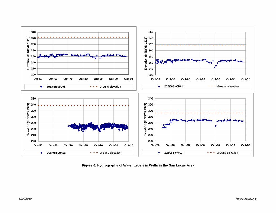
Figure 6. Hydrographs of Water Levels in Wells in the San Lucas Area

200

220

240

260

280

300

320

340

Oct-50 Oct-60 Oct-70 Oct-80 Oct-90 Oct-00 Oct-10

Elev

atio

n (ft

NG

VD 1

929)

'20S/08E-05C01' Ground elevation

220

240

260

280

300

320

340

360


Elev

atio

n (ft

NG

VD 1

929)

'20S/08E-05R03' Ground elevation

220

240

260

280

300

320

340

360


Elev

atio

n (ft

NG

VD 1

929)

'20S/08E-06K01' Ground elevation

200

220

240

260

280

300

320

340

Oct-50 Oct-60 Oct-70 Oct-80 Oct-90 Oct-00 Oct-10El

evat

ion

(ft N

GVD

192

9)

'20S/08E-07F01' Ground elevation

6/24/2010 Hydrographs.xls

Figure 6 — continued

180

200

220

240

260

280

300

320


Elev

atio

n (ft

NG

VD 1

929)

'20S/08E-09M01' Ground elevation

200

220

240

260

280

300

320

340


Elev

atio

n (ft

NG

VD 1

929)

'20S/08E-15H03' Ground elevation

200

220

240

260

280

300

320

340


Elev

atio

n (ft

NG

VD 1

929)

'20S/08E-16C01' Ground elevation

220

240

260

280

300

320

340

360


evat

ion

(ft N

GVD

192

9)

'20S/08E-25Q01' Ground elevation



300

320

340

360

380

400

420

440

460


Elev

atio

n (ft

NG

VD 1

929)

'20S/08E-34G01' Ground elevation

240

260

280

300

320

340

360

380


Elev

atio

n (ft

NG

VD 1

929)

'21S/09E-16B01' Ground elevation

240

260

280

300

320

340

360

380


Elev

atio

n (ft

NG

VD 1

929)

'21S/09E-16E01' Ground elevation

Closest well to SLCWD #2

320

340

360

380

400

420

440

460


evat

ion

(ft N

GVD

192

9)

'21S/09E-17Q01' Ground elevation



260

280

300

320

340

360

380

400


Elev

atio

n (ft

NG

VD 1

929)

'21S/09E-23G01' Ground elevation

300

320

340

360

380

400

420

440


Elev

atio

n (ft

NG

VD 1

929)

'21S/09E-24L01' Ground elevation


[

[

Wild

KCAC

Cat-1

SL-33

06C01

36R01

07E01

25Q01

16C01

08Q0208Q03

05R03

05C02

08F01

24L0124Q0122J01

16E0116E02

23G01

15H03

07F01

06B01

17K03

08M01

34G01

24J02

08D50

15J01

SL-LacSLCWD-1

SLCWD-2

San Lucas

King City

Figure 7. Map of Water Quality Wells and TDS Concentrations

R. 8 E R. 9 ET.

20

ST.

21

S ±0 2 4 61

Miles

Legend

Water level measurement well. Label is last part of state well number.

TDS concentration (mg/L)

0 - 600

600 - 1200

1200 - 1800

1600 - 2400

>2400

River channel deposits

Fluvial deposits

Paso Robles Fornation

Older rocks

!(

34G1

!(

!(

!(

!(

!(

Figure 8. Chemographs of Total Dissolved Solids Concentration in Wells in the San Lucas Area, 1970-2009

20S08E-05C02

0

500

1,000

1,500

2,000

2,500

3,000

3,500

Oct-70 Oct-74 Oct-78 Oct-82 Oct-86 Oct-90 Oct-94 Oct-98 Oct-02 Oct-06 Oct-10

Dis

solv

ed S

olid

s (m

g/L)

20S08E-05R03

0

500

1,000

1,500

2,000

2,500

3,000

3,500


Dis

solv

ed S

olid

s (m

g/L)

20S08E-08C01

0

500

1,000

1,500

2,000

2,500

3,000

3,500

Oct-70 Oct-74 Oct-78 Oct-82 Oct-86 Oct-90 Oct-94 Oct-98 Oct-02 Oct-06 Oct-10D

isso

lved

Sol

ids

(mg/

L)

20S08E-06B01

0

500

1,000

1,500

2,000

2,500

3,000

3,500


Dis

solv

ed S

olid

s (m

g/L)

6/25/2010 WQconvertOut.xls

Figure 8 C continued

20S08E-07E01

0

500

1,000

1,500

2,000

2,500

3,000

3,500


Dis

solv

ed S

olid

s (m

g/L)

20S08E-08C02

0

500

1,000

1,500

2,000

2,500

3,000

3,500


Dis

solv

ed S

olid

s (m

g/L)

20S08E-08D50

0

500

1,000

1,500

2,000

2,500

3,000

3,500


Dis

solv

ed S

olid

s (m

g/L)

20S08E-08F01

0

500

1,000

1,500

2,000

2,500

3,000

3,500


isso

lved

Sol

ids

(mg/

L)



20S08E-08M01

0

500

1,000

1,500

2,000

2,500

3,000

3,500


Dis

solv

ed S

olid

s (m

g/L)

20S08E-08Q02

0

500

1,000

1,500

2,000

2,500

3,000

3,500


Dis

solv

ed S

olid

s (m

g/L)

20S08E-08Q03

0

500

1,000

1,500

2,000

2,500

3,000

3,500


Dis

solv

ed S

olid

s (m

g/L)

20S08E-15H03

0

500

1,000

1,500

2,000

2,500

3,000

3,500


isso

lved

Sol

ids

(mg/

L)



20S08E-16C01

0

500

1,000

1,500

2,000

2,500

3,000

3,500


Dis

solv

ed S

olid

s (m

g/L)

20S08E-17K03

0

500

1,000

1,500

2,000

2,500

3,000

3,500


Dis

solv

ed S

olid

s (m

g/L)

20S08E-25Q01

0

500

1,000

1,500

2,000

2,500

3,000

3,500


Dis

solv

ed S

olid

s (m

g/L)

20S08E-34G01

0

500

1,000

1,500

2,000

2,500

3,000

3,500


isso

lved

Sol

ids

(mg/

L)



20S08E-36R01

0

500

1,000

1,500

2,000

2,500

3,000

3,500


Dis

solv

ed S

olid

s (m

g/L)

21S08E-15J01

0

500

1,000

1,500

2,000

2,500

3,000

3,500


Dis

solv

ed S

olid

s (m

g/L)

21S09E-06C01

0

500

1,000

1,500

2,000

2,500

3,000

3,500


Dis

solv

ed S

olid

s (m

g/L)

21S09E-16E02

0

500

1,000

1,500

2,000

2,500

3,000

3,500


isso

lved

Sol

ids

(mg/

L)



21S09E-22J01

0

500

1,000

1,500

2,000

2,500

3,000

3,500


Dis

solv

ed S

olid

s (m

g/L)

21S09E-23G01

0

500

1,000

1,500

2,000

2,500

3,000

3,500


Dis

solv

ed S

olid

s (m

g/L)

21S/09E-24L1 and 24Q1

0

500

1,000

1,500

2,000

2,500

3,000

3,500


isso

lved

Sol

ids

(mg/

L)

21S09E-17H1 (SLCWD #2)

0

500

1,000

1,500

2,000

2,500

3,000

3,500


Dis

solv

ed S

olid

s (m

g/L) SLCWD Well #2


200,000

400,000

600,000

800,000

1,000,000

1,200,000

1,400,000

1,600,000An

nual

Dis

char

ge (a

cre-

feet

)

8/26/2010 ^SR_nr_Bradley_5010.xls

Figure 9. Annual Discharge in the Salinas River near Bradley, water years 1950-2009

0

200,000

400,000

600,000

800,000

1,000,000

1,200,000

1,400,000

1,600,000

1951

1953

1955

1957

1959

1961

1963

1965

1967

1969

1971

1973

1975

1977

1979

1981

1983

1985

1987

1989

1991

1993

1995

1997

1999

2001

2003

2005

2007

2009

Annu

al D

isch

arge

(acr

e-fe

et)

Water Year

8/26/2010 ^SR_nr_Bradley_5010.xls

Figure 10. Trilinear (Piper) Plot of Groundwater Quality in the San Lucas Area

[

[San Lucas

King City

Figure 11. Map of Groundwater Quality Composition in the San Lucas Area

R. 8 E R. 9 ET.

20

ST.

21

S ±0 2 4 61

Miles

Legend

Water Quality Composition

Group 2

Group 3

Group 4

Group 5

Group 6

Surficial Geology River channel deposits

Fluvial deposits

Paso Robles Formation

Older rocks

!(

!(

!(

!(

!(

0

500

1000

1500

2000

2500

3000

3500

A B C D EWater Quality Group

SalinasRiver

Poncho RicoFormation

Figure 12. Boxplots of Total Dissolved Solids Concentration in Water Quality Groups

2 3 4 5 6

1981-19981999-20052006-2009

\

SLCWD Well #2

Auger holes

2009

\

\

\\\\

Figure 13. Composition of Groundwater at SLCWD Well #2 and Nearby Water Table Auger Holes

Figure 14. Deuterium and O-18 Composition of Water Samples in the San Lucas Area

-80

-70

-60

-50

-40

-30

-20

-10

0

-10 -8 -6 -4 -2 0Delta O-18

Del

ta D 1 and 4

3

52

6

Site Descriptions1 Ag well near SLCWD #22 Water table next to SLCWD #23 Salinas River4 SLCWD #25 Water table between SLCWD #2 and Salinas River6 San Lucas School irrigation well

Global meteoric water line

6/25/2010 Isotope_samples.xls

Figure 15a. Aerial Photograph of the Floodplain Area near Well SLCWD #2, May 10, 1994

SLCWD #2

San Lucas

Figure 15b. Aerial Photograph of the Floodplain Area near Well SLCWD #2, August 30, 2004

SLCWD #2

San Lucas

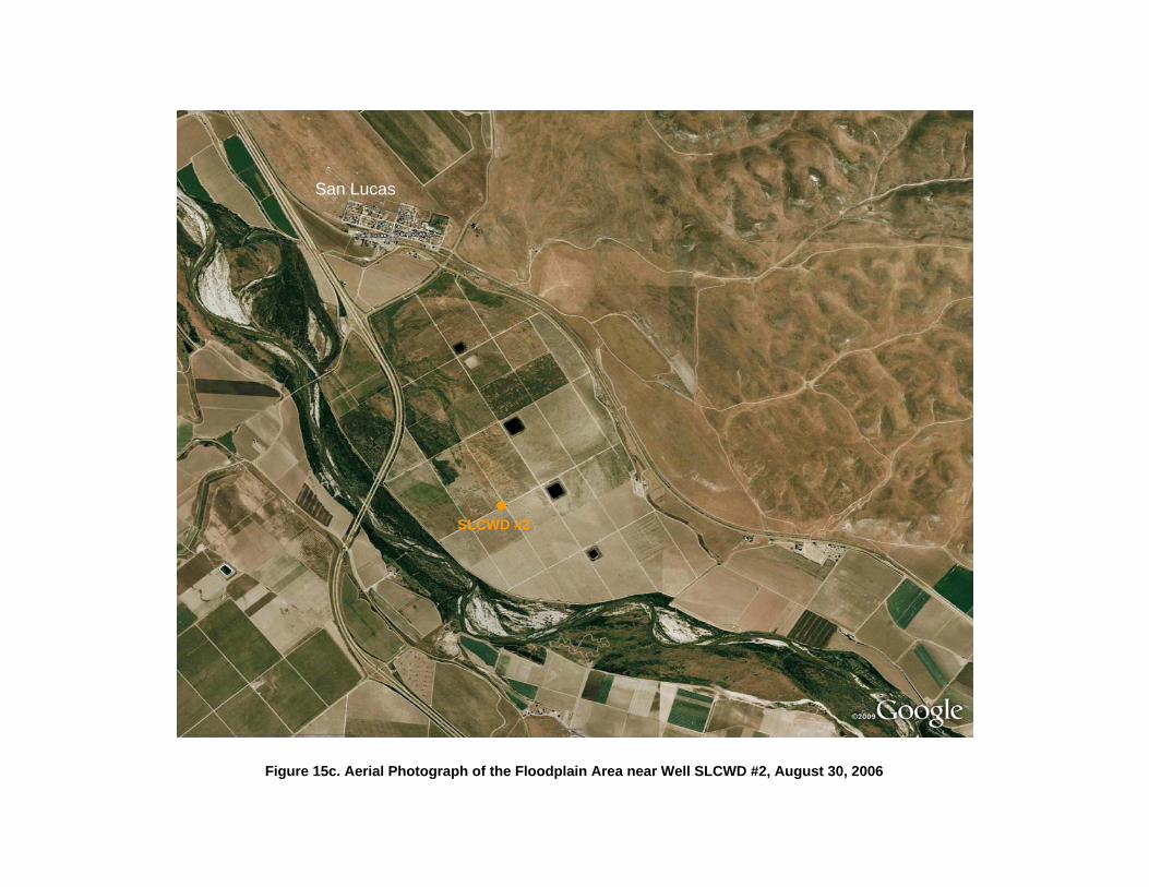
Figure 15c. Aerial Photograph of the Floodplain Area near Well SLCWD #2, August 30, 2006

SLCWD #2

San Lucas

Figure 15d. Aerial Photograph of the Floodplain Area near Well SLCWD #2, July 30, 2007

SLCWD #2

San Lucas

Figure 15e. Aerial Photograph of the Floodplain Area near Well SLCWD #2, May 25, 2009

SLCWD #2

San Lucas

HYDROGEOLOGIC CHARACTERIZATION AND TEST WELL FEASIBILITY ...

Documents

Transcript of HYDROGEOLOGIC CHARACTERIZATION AND TEST WELL FEASIBILITY ...