
Hydrogen Gas Retention and Release from WTP Vessels ... · Hydrogen Gas Retention and Release from...
240
PNNL-24255 WTP-RPT-238 Rev. 0 Prepared for the U.S. Department of Energy under Contract DE-AC05-76RL01830 Hydrogen Gas Retention and Release from WTP Vessels: Summary of Preliminary Studies July 2015 PA Gauglitz GK Boeringa JR Bontha WC Buchmiller RC Daniel CA Burns LA Mahoney J Chun SD Rassat NK Karri BE Wells H Li J Bao DN Tran
Transcript of Hydrogen Gas Retention and Release from WTP Vessels ... · Hydrogen Gas Retention and Release from...

PNNL-24255 WTP-RPT-238 Rev. 0
Prepared for the U.S. Department of Energy under Contract DE-AC05-76RL01830
Hydrogen Gas Retention and Release from WTP Vessels: Summary of Preliminary Studies
July 2015
PA Gauglitz GK Boeringa
JR Bontha WC Buchmiller
RC Daniel CA Burns
LA Mahoney J Chun
SD Rassat NK Karri
BE Wells H Li
J Bao DN Tran
DISCLAIMER
This report was prepared as an account of work sponsored by an agency of the
United States Government. Neither the United States Government nor any agency
thereof, nor Battelle Memorial Institute, nor any of their employees, makes any
warranty, express or implied, or assumes any legal liability or responsibility for
the accuracy, completeness, or usefulness of any information, apparatus,
product, or process disclosed for any uses other than those related to WTP for DOE,
or represents that its use would not infringe privately owned rights. Reference
herein to any specific commercial product, process, or service by trade name,
trademark, manufacturer, or otherwise does not necessarily constitute or imply its
endorsement, recommendation, or favoring by the United States Government or any
agency thereof, or Battelle Memorial Institute. The views and opinions of authors
expressed herein do not necessarily state or reflect those of the United States
Government or any agency thereof.
PACIFIC NORTHWEST NATIONAL LABORATORY
operated by
BATTELLE for the
UNITED STATES DEPARTMENT OF ENERGY
under Contract DE-AC05-76RL01830
Printed in the United States of America
Available to DOE and DOE contractors from the Office of Scientific and Technical Information,
P.O. Box 62, Oak Ridge, TN 37831-0062; ph: (865) 576-8401 fax: (865) 576-5728
email: reports@adonis,osti.gov
Available to the public from the National Technical Information Service 5301 Shawnee Rd., Alexandria, VA 22312
ph: (800) 553-NTIS (6847) email: [email protected] <http://www.ntis.gov/about/form.aspx>
This document was printed on recycled paper.
(9/2003)
PNNL-24255
WTP-RPT-238 Rev. 0
Hydrogen Gas Retention and Release from WTP Vessels: Summary of Preliminary Studies
PA Gauglitz GK Boeringa
JR Bontha WC Buchmiller
RC Daniel CA Burns
LA Mahoney J Chun
SD Rassat NK Karri
BE Wells H Li
J Bao DN Tran
July 2015
Test Specification: NA
Work Authorization: WA-50
Test Plan: NA
Test Exceptions: NA
Prepared for
the U.S. Department of Energy
under Contract DE-AC05-76RL01830
Pacific Northwest National Laboratory
Richland, Washington 99352


iii
Summary
The Hanford Waste Treatment and Immobilization Plant (WTP) is currently being designed and
constructed to pretreat and vitrify a large portion of the waste in the 177 underground waste storage tanks
at the Hanford Site. A number of technical issues related to the design of the pretreatment facility (PTF)
of the WTP have been identified. These issues must be resolved prior to the U.S. Department of Energy
(DOE) Office of River Protection (ORP) reaching a decision to proceed with engineering, procurement,
and construction activities for the PTF. One of the issues is Technical Issue T1 - Hydrogen Gas Release
from Vessels (hereafter referred to as T1). The focus of T1 is identifying controls for hydrogen release
and completing any testing required to close the technical issue.
In advance of selecting specific controls for hydrogen gas safety, a number of preliminary technical
studies were initiated to support anticipated future testing and to improve the understanding of hydrogen
gas generation, retention, and release within PTF vessels. These activities supported the development of a
plan defining an overall strategy and approach for addressing T1 and achieving technical endpoints
identified for T1. Preliminary studies also supported the development of a test plan for conducting testing
and analysis to support closing T1. Both of these plans were developed in advance of selecting specific
controls, and in the course of working on T1 it was decided that the testing and analysis identified in the
test plan were not immediately needed. However, planning activities and preliminary studies led to
significant technical progress in a number of areas. This report summarizes the progress to date from the
preliminary technical studies. The technical results in this report should not be used for WTP design or
safety and hazards analyses and technical results are marked with the following statement: “Preliminary
Technical Results for Planning – Not to be used for WTP Design or Safety Analyses.”
S.1 Objectives
The overall objective of the preliminary studies discussed in this report was to prepare for developing
detailed technical plans for addressing key issues for closing T1 and the preliminary studies and plans
assumed pulse jet mixer (PJM) mixing was the active method for releasing hydrogen gas. The key
technical questions that were the focus of future testing and analysis being supported by the preliminary
studies included the following:
What is an appropriate mixing metric/requirement that corresponds to adequate gas release and can
this requirement be used as an alternative to conducting gas release testing?
Do the simulants used in previous gas release testing adequately represent actual waste at plant
conditions and what is the most suitable simulant for any planned gas release testing?
What is the quantity of hydrogen that could be retained and released during normal, abnormal, and
post-design-basis event operations for a range of imperfect mixing conditions (i.e., how much margin
is allowed in targeting complete bottom clearing and complete vessel motion)?
What is the quantity of hydrogen that can be retained and released in low-solids vessels?
What is the margin in the current hydrogen generation rate estimates?
Specific test and analysis objectives were identified for each of these questions and subsequently
documented in a test plan; however, no technical activities were completed under the test plan for
addressing these technical questions.
iv
S.2 Results and Performance Against Success Criteria
Success criteria were developed for each testing and analysis objective and documented in the project test
plan; however, no technical activities were completed on the objectives under the test plan. Accordingly,
no results are available to compare against the success criteria.
S.3 Quality Requirements
The Pacific Northwest National Laboratory (PNNL) Quality Assurance (QA) Program is based upon the
requirements as defined in DOE Order 414.1D, Quality Assurance and Title 10 of the Code of Federal
Regulations (CFR) Part 830, Energy/Nuclear Safety Management, Subpart A -- Quality Assurance
Requirements (a.k.a. the Quality Rule). PNNL has chosen to implement the following consensus
standards in a graded approach:
ASME NQA-1-2000, Quality Assurance Requirements for Nuclear Facility Applications, Part 1,
Requirements for Quality Assurance Programs for Nuclear Facilities
ASME NQA-1-2000, Part II, Subpart 2.7, Quality Assurance Requirements for Computer Software
for Nuclear Facility Applications
ASME NQA-1-2000, Part IV, Subpart 4.2, Graded Approach Application of Quality Assurance
Requirements for Research and Development.
The procedures necessary to implement the requirements are documented through PNNL’s “How Do
I…?” (HDI), a standards-based system for managing the delivery of laboratory-level policies,
requirements, and procedures.
The work described in this report was conducted under the current QA program document revision
previously submitted to Bechtel National, Inc. (BNI): Quality Assurance Manual QA-WTPSP-0002
Rev 1.1; Quality Assurance Plan QA-WTPSP-0001 Rev 2.0; Quality Assurance Requirements Matrix
(QARM) QA-WTPSP-0003 Rev 2.0. The QA plan for the Waste Treatment Plant Support Project
(WTPSP) implements the requirements of ASME NQA 1 2000, Part 1: Requirements for Quality
Assurance Programs for Nuclear Facilities, presented in two parts. Part 1 of the QA Manual describes the
graded approach developed by applying NQA 1 2000, Subpart 4.2, Guidance on Graded Application of
Quality Assurance (QA) for Nuclear-Related Research and Development to the requirements based on the
type of work scope the WTPSP is facing. Part 2 of the QA Manual lists all of the NQA-1-2000
requirements that the project is implementing for the different technology levels of Research and
Development (R&D) work. Applicable requirements are clearly listed for each technology level.
The WTPSP uses a graded approach for the application of QA controls such that the level of analysis,
extent of documentation, and degree of rigor of process control are applied commensurate with their
significance, importance to safety, life cycle state of work, or programmatic mission. The work described
in this report has been completed at the QA technology level of Basic Research, which is the lowest QA
technology level. This level was selected because the purpose of the preliminary studies was to support
planning. The technical results in this report should not be used for WTP design or safety and hazards
analyses and technical results are marked with the following statement: “Preliminary Technical Results
for Planning – Not to be used for WTP Design or Safety Analyses.”
v
S.4 Simulant Use
A range of simulants were used for the preliminary studies. The simulants were selected to evaluate their
potential use in future testing and no efforts were made to match their properties to actual waste.
S.5 Summary of Preliminary Results
Technical results were analyzed and progress was made toward developing technical approaches for
addressing each key technical question (see Section S.1). Summaries of these results are presented below.
As noted in Section S.3, these results are “Preliminary Technical Results for Planning – Not to be used for
WTP Design or Safety Analyses.”
Develop Mixing Metric/Requirement (MR) for Gas Release and Demonstrate in Small-Scale Testing
Velocity Sensor Evaluation – Two different velocity sensors were evaluated to determine their ability
to quantify the motion of clay slurries having Bingham yield stress in the target range of 6 to 30 Pa
with the ultimate objective of being able to correlate gas release to the motion of a non-Newtonian
yield-stress fluid near the surface of a PJM mixed vessel. The first sensor, a Met-Flow Ultrasonic
Velocity Profiler (UVP) Model: UVP-DUO with a 2 MHz transducer (both from Met-Flow SA), was
found to be more sensitive to fluid motion and had fewer issues with solids build up because the
measuring range extended beyond the stagnant region of yield stress fluid that occurs near the sensor
surface. The second sensor was a Valeport 802 2-Axis Electromagnetic (EM) current meter (Seafloor
Systems). Although it was sensitive to fluid motion, its response became unreliable after a stagnant
region of solids built up in the measuring volume near the sensor surface. Further, based on limited
preliminary studies, the UVP-DUOOU/2 MHz transducer combination appeared to be more suitable
for correlating gas release with fluid motion. However, tests were not completed to determine if a
clear correlation exists between fluid motion, as measured by the sensor, and gas release.
Radio-Frequency Identification (RFID) Tag Development and Evaluation – A method was developed
to make buoyant RFID beads of approximately 1 cm in diameter and with a range of densities. The
density was adjusted from about 0.6 to 1.2 g/mL to allow the beads, which are thought to be larger
than typical retained gas bubbles, to have buoyant motion that more closely mimics the motion of
smaller, but lower density, gas bubbles. Tag release tests conducted in a small mechanically agitated
vessel indicated that, within the range tested, the onset of tag release was not a function of tag density.
Results indicated that once surface shear was observed the beads would release to the surface. Tests
were not completed to determine a preferred RFID tag density that would give a clear correlation
between tag release and gas release when the slurry is sheared.
PJM Test Stand for Evaluating Gas Release Metrics – A 42 in. diameter clear acrylic vessel with a
nearly elliptical bottom was selected as an appropriate vessel size for conducting PJM tests with gas
release together with flow sensor measurements and RFID beads. A vendor fabricated the vessel, but
no testing was conducted.
Evaluate Flammable Gas Consequence of Imperfect Mixing
Regions of imperfect mixing are identified as dead zones where the absence of fluid motion allows
hydrogen gas to be retained and potentially spontaneously released when the gas retention becomes
sufficiently large. Preliminary calculations of the buoyant motion of dead zones in un-sheared
non-Newtonian yield-stress fluid provided insight into the approximate effects of potential behavior.
Preliminary results included estimating the allowable dead zone size where releases will not exceed
25 percent of the lower flammability limit (LFL) for hydrogen in vessel headspaces. Different
modeling approaches were compared and the comparison showed significant uncertainties in these

vi
approaches. In addition, preliminary estimates were compared to preliminary test data. Given the
range of possible behavior, reasonably accurate estimates for gas releases will need specific test data
for the scenarios and conditions representative of Hanford waste. Hanford waste exhibits a wide
range of behaviors significant to gas retention and release, and the effect of PTF treatment processes
on these behaviors is not well understood. Thus, a robust mixing system will likely be required to
keep dead zones and the potential gas inventory sufficiently small during normal operations.
Simulant Selection for Quantifying Gas Release in Testing and Comparison to Actual Waste Behavior
A concept was developed for a bench-scale apparatus for comparing gas release behavior of different
simulants under controlled shearing. The intent of the apparatus was that it could also be adapted for
testing small samples of actual waste in a hot cell using remote manipulators. The conceptual
apparatus was not fabricated and, thus, not used in testing. As part of the preliminary planning, an
actual waste sample was selected for testing (i.e., AY-102) and a technical justification prepared for
the use of this sample in gas release testing.
Previous studies have shown different gas release behavior for simulants composed of different clay
materials, specifically materials with different proportions of kaolin and bentonite clays. Previous
work has also shown that the generation rate of oxygen bubbles from the decomposition of hydrogen
peroxide depends on the proportions of kaolin and bentonite and on the pH of the slurry. To support
the selection of a simulant for future gas release testing, Bingham parameters, shear strength (vane
method), gas generation rate with hydrogen peroxide, and settling behavior were evaluated for a
number of clay slurries with proportions of kaolin and bentonite varying from 80 weight percent
(wt%) kaolin and 20 wt% bentonite (80:20 K:B) to 100:0 K:B. For these simulant development and
characterization activities, the magnitude of the Bingham parameters was varied over a range by
adjusting the weight fraction of the clay in water-based slurries. Correlations developed from this
work were used to specify simulant recipes to target properties for use in preliminary gas release
testing.
Experimental Investigations of Bubble Cascade, Buoyant Displacement, Dead Zone, and Induced Gas
Releases from Non-Newtonian Simulants and Settling Solids Layers
Spontaneous Bubble Cascade (BC) Gas Releases – A review and summary of existing BC release
data was completed. This summary includes documentation of a BC gas release event in a PJM test
system that was conducted as part of a previous study but never reported. A comparison of the data
shows similarity in behavior from the different studies in which somewhat different simulants and test
conditions were used. The summary shows very few test data exist for materials with rheology in the
expected range for WTP non-Newtonian slurries (Bingham yield stress between 6 and 30 Pa and
consistency between 6 and 30 cP), particularly at the low end.
Spontaneous and Induced Gas Releases from Non-Newtonian Simulants – A conceptual approach
was developed for conducting tests to evaluate the onset of dead zone motion and the quantity of gas
released from a hypothetical dead zone. A single preliminary experiment was conducted where an
annular region at the bottom of a test vessel (simulated dead zone) included hydrogen peroxide to
generate retained gas bubbles over a period of about 25 hours. The preliminary results estimated the
retained gas fraction at the onset of motion, which occurred after ~15 hours, and the fraction of
retained gas that was released. Tests were also conducted to evaluate gas retention and release in
non-Newtonian slurries when only a single gas sparger placed near the bottom of the vessel was
operated at low-flow rate. Test observations suggested that gas was released near the sparger, where
injected gas moved vertically through the slurry in a “region of bubbles”, and that the removal of in
situ generated gas induced a slow motion away from the sparger due to the buoyancy difference
between the region where in situ gas was removed by sparging and the region that had higher retained
vii
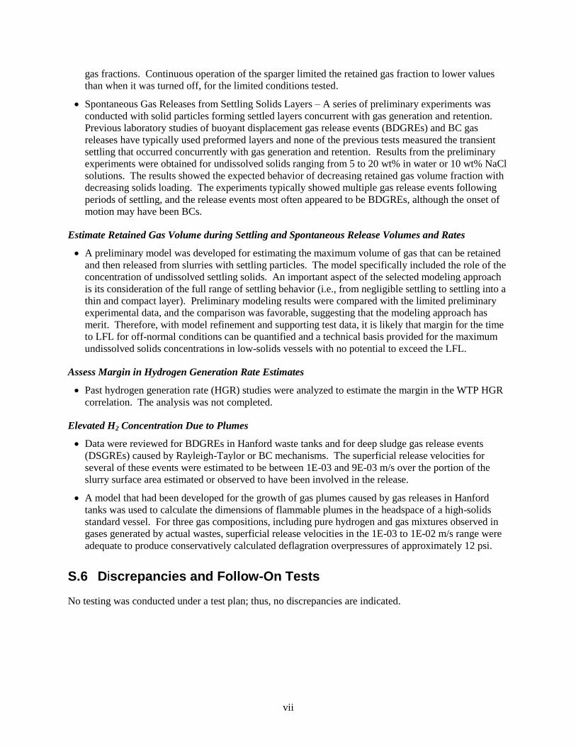
gas fractions. Continuous operation of the sparger limited the retained gas fraction to lower values
than when it was turned off, for the limited conditions tested.
Spontaneous Gas Releases from Settling Solids Layers – A series of preliminary experiments was
conducted with solid particles forming settled layers concurrent with gas generation and retention.
Previous laboratory studies of buoyant displacement gas release events (BDGREs) and BC gas
releases have typically used preformed layers and none of the previous tests measured the transient
settling that occurred concurrently with gas generation and retention. Results from the preliminary
experiments were obtained for undissolved solids ranging from 5 to 20 wt% in water or 10 wt% NaCl
solutions. The results showed the expected behavior of decreasing retained gas volume fraction with
decreasing solids loading. The experiments typically showed multiple gas release events following
periods of settling, and the release events most often appeared to be BDGREs, although the onset of
motion may have been BCs.
Estimate Retained Gas Volume during Settling and Spontaneous Release Volumes and Rates
A preliminary model was developed for estimating the maximum volume of gas that can be retained
and then released from slurries with settling particles. The model specifically included the role of the
concentration of undissolved settling solids. An important aspect of the selected modeling approach
is its consideration of the full range of settling behavior (i.e., from negligible settling to settling into a
thin and compact layer). Preliminary modeling results were compared with the limited preliminary
experimental data, and the comparison was favorable, suggesting that the modeling approach has
merit. Therefore, with model refinement and supporting test data, it is likely that margin for the time
to LFL for off-normal conditions can be quantified and a technical basis provided for the maximum
undissolved solids concentrations in low-solids vessels with no potential to exceed the LFL.
Assess Margin in Hydrogen Generation Rate Estimates
Past hydrogen generation rate (HGR) studies were analyzed to estimate the margin in the WTP HGR
correlation. The analysis was not completed.
Elevated H2 Concentration Due to Plumes
Data were reviewed for BDGREs in Hanford waste tanks and for deep sludge gas release events
(DSGREs) caused by Rayleigh-Taylor or BC mechanisms. The superficial release velocities for
several of these events were estimated to be between 1E-03 and 9E-03 m/s over the portion of the
slurry surface area estimated or observed to have been involved in the release.
A model that had been developed for the growth of gas plumes caused by gas releases in Hanford
tanks was used to calculate the dimensions of flammable plumes in the headspace of a high-solids
standard vessel. For three gas compositions, including pure hydrogen and gas mixtures observed in
gases generated by actual wastes, superficial release velocities in the 1E-03 to 1E-02 m/s range were
adequate to produce conservatively calculated deflagration overpressures of approximately 12 psi.
S.6 Discrepancies and Follow-On Tests
No testing was conducted under a test plan; thus, no discrepancies are indicated.


ix
Acknowledgments
The authors would like to thank Phil Schonewill for his careful technical review and Sam Bryan, Don
Camaioni, Bojana Ginovska-Pangovska, Rich Pires, Kurt Recknagle, and Sarah Suffield for their
technical contributions to the initial project planning and preliminary progress reported here. We would
also like to thank Kirsten Meier for her guidance on Quality Assurance matters, Mike Parker for his
helpful editing, and Chrissy Charron and Mona Champion for their overall administrative support.
Funding for this effort was provided by both the U.S. Department of Energy’s Hanford Waste Treatment
and Immobilization Plant Project and the U.S. Department of Energy’s Office of River Protection.

xi
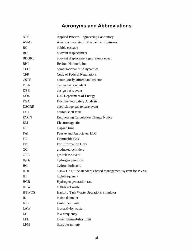
Acronyms and Abbreviations
APEL Applied Process Engineering Laboratory
ASME American Society of Mechanical Engineers
BC bubble cascade
BD buoyant displacement
BDGRE buoyant displacement gas release event
BNI Bechtel National, Inc.
CFD computational fluid dynamics
CFR Code of Federal Regulations
CSTR continuously stirred tank reactor
DBA design basis accident
DBE design basis event
DOE U.S. Department of Energy
DSA Documented Safety Analysis
DSGRE deep-sludge gas release event
DST double-shell tank
ECCN Engineering Calculation Change Notice
EM Electromagnetic
ET elapsed time
FAI Fauske and Associates, LLC
FG Flammable Gas
FIO For Information Only
GC graduated cylinders
GRE gas release event
H2O2 hydrogen peroxide
HCl hydrochloric acid
HDI “How Do I,” the standards-based management system for PNNL
HF high-frequency
HGR Hydrogen generation rate
HLW high-level waste
HTWOS Hanford Task Waste Operations Simulator
ID inside diameter
K:B kaolin:bentonite
LAW low-activity waste
LF low-frequency
LFL lower flammability limit
LPM liters per minute
xii
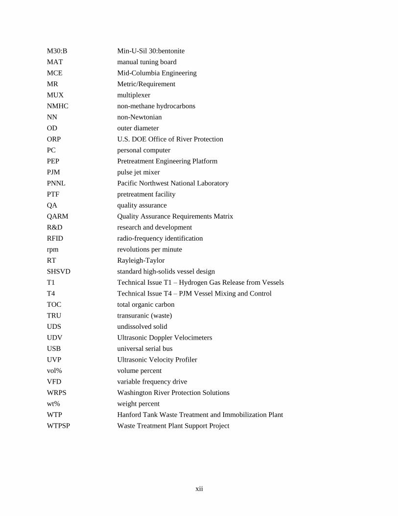
M30:B Min-U-Sil 30:bentonite
MAT manual tuning board
MCE Mid-Columbia Engineering
MR Metric/Requirement
MUX multiplexer
NMHC non-methane hydrocarbons
NN non-Newtonian
OD outer diameter
ORP U.S. DOE Office of River Protection
PC personal computer
PEP Pretreatment Engineering Platform
PJM pulse jet mixer
PNNL Pacific Northwest National Laboratory
PTF pretreatment facility
QA quality assurance
QARM Quality Assurance Requirements Matrix
R&D research and development
RFID radio-frequency identification
rpm revolutions per minute
RT Rayleigh-Taylor
SHSVD standard high-solids vessel design
T1 Technical Issue T1 – Hydrogen Gas Release from Vessels
T4 Technical Issue T4 – PJM Vessel Mixing and Control
TOC total organic carbon
TRU transuranic (waste)
UDS undissolved solid
UDV Ultrasonic Doppler Velocimeters
USB universal serial bus
UVP Ultrasonic Velocity Profiler
vol% volume percent
VFD variable frequency drive
WRPS Washington River Protection Solutions
wt% weight percent
WTP Hanford Tank Waste Treatment and Immobilization Plant
WTPSP Waste Treatment Plant Support Project
xiii
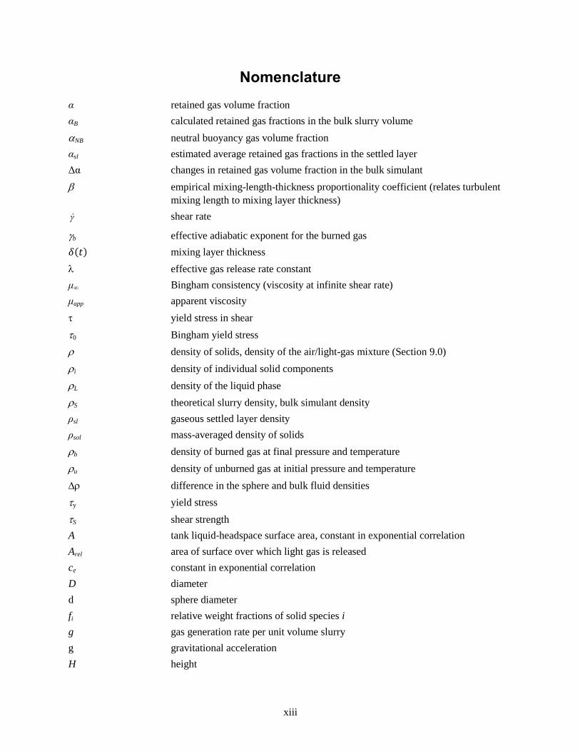
Nomenclature
α retained gas volume fraction
αB calculated retained gas fractions in the bulk slurry volume
NB neutral buoyancy gas volume fraction
αsl estimated average retained gas fractions in the settled layer
Δα changes in retained gas volume fraction in the bulk simulant
empirical mixing-length-thickness proportionality coefficient (relates turbulent
mixing length to mixing layer thickness)
shear rate
b effective adiabatic exponent for the burned gas
𝛿(𝑡) mixing layer thickness
effective gas release rate constant
μ∞ Bingham consistency (viscosity at infinite shear rate)
μapp apparent viscosity
yield stress in shear
0 Bingham yield stress
density of solids, density of the air/light-gas mixture (Section 9.0)
i density of individual solid components
L density of the liquid phase
S theoretical slurry density, bulk simulant density
ρsl gaseous settled layer density
ρsol mass-averaged density of solids
b density of burned gas at final pressure and temperature
u density of unburned gas at initial pressure and temperature
difference in the sphere and bulk fluid densities
y yield stress
S shear strength
A tank liquid-headspace surface area, constant in exponential correlation
Arel area of surface over which light gas is released
ce constant in exponential correlation
D diameter
d sphere diameter
fi relative weight fractions of solid species i
g gas generation rate per unit volume slurry
g gravitational acceleration
H height
xiv
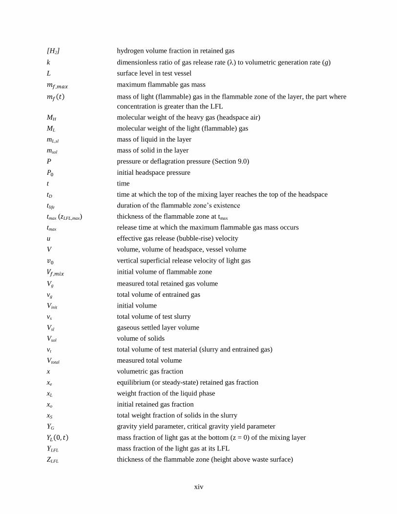
[H2] hydrogen volume fraction in retained gas
k dimensionless ratio of gas release rate () to volumetric generation rate (g)
L surface level in test vessel
𝑚𝑓,𝑚𝑎𝑥 maximum flammable gas mass
𝑚𝑓(𝑡) mass of light (flammable) gas in the flammable zone of the layer, the part where
concentration is greater than the LFL
MH molecular weight of the heavy gas (headspace air)
ML molecular weight of the light (flammable) gas
mL,sl mass of liquid in the layer
msol mass of solid in the layer
P pressure or deflagration pressure (Section 9.0)
𝑃0 initial headspace pressure
t time
tD time at which the top of the mixing layer reaches the top of the headspace
tlife duration of the flammable zone’s existence
tmax (zLFL,max) thickness of the flammable zone at tmax
tmax release time at which the maximum flammable gas mass occurs
u effective gas release (bubble-rise) velocity
V volume, volume of headspace, vessel volume
𝑣0 vertical superficial release velocity of light gas
𝑉𝑓,𝑚𝑖𝑥 initial volume of flammable zone
Vg measured total retained gas volume
vg total volume of entrained gas
Vinit initial volume
vs total volume of test slurry
Vsl gaseous settled layer volume
Vsol volume of solids
vt total volume of test material (slurry and entrained gas)
Vtotal measured total volume
x volumetric gas fraction
xe equilibrium (or steady-state) retained gas fraction
xL weight fraction of the liquid phase
xo initial retained gas fraction
xS total weight fraction of solids in the slurry
YG gravity yield parameter, critical gravity yield parameter
𝑌𝐿(0, 𝑡) mass fraction of light gas at the bottom (z = 0) of the mixing layer
YLFL mass fraction of the light gas at its LFL
ZLFL thickness of the flammable zone (height above waste surface)

xv
Subscripts
b bubble
DZ dead zone
W waste
HS headspace

xvii
Contents
Summary ...................................................................................................................................................... iii
Acknowledgments ........................................................................................................................................ ix
Acronyms and Abbreviations ...................................................................................................................... xi
Nomenclature ............................................................................................................................................. xiii
Subscripts .................................................................................................................................................... xv
1.0 Introduction ...................................................................................................................................... 1.1
1.1 Objectives ............................................................................................................................... 1.1
1.2 Background on Gas Retention and Release in Vessels Using Pulse Jet Mixing .................... 1.2
2.0 Quality Assurance ............................................................................................................................ 2.1
3.0 Develop Mixing Metric/Requirement (MR) for Gas Release and Demonstrate in Small-
Scale Testing .................................................................................................................................... 3.1
3.1 Objectives and Success Criteria ............................................................................................. 3.1
3.2 Technical Approach ............................................................................................................... 3.2
3.3 RFID Tag Development ......................................................................................................... 3.4
3.3.1 Types of RFID Beads ................................................................................................ 3.4
3.3.2 RFID Bead Fabrication Methods .............................................................................. 3.6
3.3.3 RFID Bead Fabrication Results ................................................................................. 3.9
3.3.4 Scalability of the RFID Setup to 16-ft ..................................................................... 3.12
3.3.5 Summary of RFID Tag Development Accomplishments to Date ........................... 3.13
3.4 Flow Sensors ........................................................................................................................ 3.13
3.4.1 Met-Flow UVP ........................................................................................................ 3.13
3.4.2 Valeport EM Sensors............................................................................................... 3.14
3.5 Bench-Scale Evaluation ....................................................................................................... 3.14
3.5.1 Shakedown Tests ..................................................................................................... 3.19
3.5.2 Flow Instrument Tests ............................................................................................. 3.21
3.5.3 Refined Test Procedure ........................................................................................... 3.27
3.5.4 Preliminary Bench-Scale Tests ............................................................................... 3.28
3.5.5 Summary of Key Observations and Recommendations .......................................... 3.30
3.6 Conclusions .......................................................................................................................... 3.31
4.0 Evaluate Flammable Gas Consequence of Imperfect Mixing ......................................................... 4.1
4.1 Objectives ............................................................................................................................... 4.2
4.2 Spontaneous Releases from Regions of Imperfect Mixing .................................................... 4.2
4.3 Preliminary Modeling Approach, Results, and Comparison to Test Data ............................. 4.5
5.0 Simulant Selection for Quantifying Gas Release in Testing and Comparison to Actual
Waste Behavior ................................................................................................................................ 5.1
5.1 Test Objectives and Success Criteria ..................................................................................... 5.1
5.2 Technical Approach ............................................................................................................... 5.2

xviii
5.3 Actual Waste Testing Recommendations ............................................................................... 5.4
5.4 Models for Interpreting Gas Release Rates and Steady-State Holdup ................................... 5.6
5.5 Preliminary Development and Characterization of Non-Newtonian Simulants for Gas
Release Studies ..................................................................................................................... 5.10
5.5.1 Simulant Preparation ............................................................................................... 5.10
5.5.2 Simulant Characterization ....................................................................................... 5.13
5.5.3 Non-Newtonian Simulant Properties ....................................................................... 5.16
6.0 Experimental Investigations of Bubble Cascade, Buoyant Displacement, Dead Zone, and
Induced Gas Releases from Non-Newtonian Simulants and Settling Solids Layers ....................... 6.1
6.1 Spontaneous Bubble-Cascade Gas Releases .......................................................................... 6.1
6.1.1 Objective and Success Criteria .................................................................................. 6.1
6.1.2 Technical Approach .................................................................................................. 6.2
6.1.3 Background ............................................................................................................... 6.2
6.1.4 Historical Bubble-Cascade Data ............................................................................... 6.3
6.2 Experimental Methods and Systems for Gas Release Investigations ................................... 6.10
6.2.1 Test Facilities and Equipment ................................................................................. 6.10
6.2.2 Conducting Tests ..................................................................................................... 6.13
6.2.3 Data Analysis .......................................................................................................... 6.14
6.3 Spontaneous and Induced Gas Releases from Non-Newtonian Simulants .......................... 6.16
6.3.1 Objectives and Success Criteria .............................................................................. 6.16
6.3.2 Test Overview ......................................................................................................... 6.17
6.3.3 Gas Release from a Dead Zone ............................................................................... 6.19
6.3.4 Induced Gas Release Using a Single Air Sparger ................................................... 6.22
6.3.5 Induced Gas Release Using Mechanical Agitators ................................................. 6.27
6.4 Spontaneous Gas Releases from Settling Solids Layers ...................................................... 6.28
6.4.1 Objectives and Success Criteria .............................................................................. 6.28
6.4.2 Results for Gas Retention and Releases with Settling Layers ................................. 6.29
7.0 Estimate Retained Gas Volume During Settling and Spontaneous Release Volumes and
Rates ................................................................................................................................................. 7.1
7.1 Objectives ............................................................................................................................... 7.1
7.2 Preliminary Modeling Approach, Results, and Comparison to Test Data ............................. 7.2
8.0 Assess Margin in Hydrogen Generation Rate Estimates.................................................................. 8.1
8.1 Objectives ............................................................................................................................... 8.1
8.2 Technical Approach and Progress .......................................................................................... 8.2
9.0 Elevated H2 Concentration Due to Plumes....................................................................................... 9.1
9.1 Objectives ............................................................................................................................... 9.1
9.2 Technical Approach ............................................................................................................... 9.1
9.3 Transient Global Release Mixed-Layer Model ...................................................................... 9.2
9.4 Steady-State Local-Release Plume Model ............................................................................. 9.4
xix
9.5 Questions About the Model Assumptions .............................................................................. 9.5
9.5.1 Headspace Aspect Ratio ............................................................................................ 9.5
9.5.2 Existing Headspace Convection, Free or Forced ...................................................... 9.6
9.5.3 Denser-Than-Air Gas Releases ................................................................................. 9.6
9.6 Inputs ...................................................................................................................................... 9.6
9.6.1 Release Velocity ........................................................................................................ 9.6
9.6.2 Release-Gas Properties .............................................................................................. 9.8
9.7 Results .................................................................................................................................... 9.9
10.0 Conclusions .................................................................................................................................... 10.1
11.0 References ...................................................................................................................................... 11.1
Appendix A – Specification Sheets for Flow Sensors .............................................................................. A.1
Appendix B – Draft Notes for 6/27/14 Meeting ........................................................................................B.1
Appendix C – Evaluation of Shape Effect for the Buoyant Motion of Dead Zones in Non-
Newtonian Yield-Stress Slurries ......................................................................................................C.1
Appendix D – Non-Newtonian Simulant Properties ................................................................................. D.1
Appendix E – Proposed 23 in. Diameter Vessel Design ............................................................................ E.1
Appendix F – A Summary of Settling and Rheology Model Work ........................................................... F.1
xx
Figures
1.1. Conceptual waste configurations for a range of settling behavior and rheology ............................. 1.3
1.2. PJM mixing and gas release mechanisms from surface of vessel and dead zone with no gas
release .............................................................................................................................................. 1.3
3.1. Conceptual apparatus with controlled shearing for correlating bubble release with flow
sensor and RFID bead response ....................................................................................................... 3.3
3.2. Conceptual PJM mixed vessel for correlating bubble release with flow sensor and RFID
bead response ................................................................................................................................... 3.4
3.3. Photos of investigated LF and HF tags and their antennas .............................................................. 3.5
3.4. Illustration of the LF and HF RFID beads ....................................................................................... 3.6
3.5. Silicone rubber mold used for making RFID beads ......................................................................... 3.7
3.6. Photo of a RFID bead developed for this study ............................................................................. 3.10
3.7. Illustration of the read range of the RFID beads ............................................................................ 3.10
3.8. Illustration of a moving RFID tag in the electromagnetic field of a reader's antenna ................... 3.12
3.9. Proposed system configuration for a 16 ft diameter tank............................................................... 3.13
3.10. Bench-scale test stand used for mixing metric development ......................................................... 3.15
3.11. RFID components: (a) LF RFID beads of different densities, (b) LF RFID reader and
display meter .................................................................................................................................. 3.16
3.12. (a) Two-axis EM flow sensor, (b) 2 MHz UVP transducer ........................................................... 3.17
3.13. Representative location of RFID beads in the bench-scale test tank ............................................. 3.18
3.14. X-axis velocity in the tank measured by Valeport EM flow sensor ............................................... 3.22
3.15. Y-axis velocity in the tank measured by Valeport EM flow sensor ............................................... 3.23
3.16. Magnified x-axis (circumferential) velocity in the tank measured by Valeport EM flow
sensor ............................................................................................................................................. 3.23
3.17. Magnified y-axis velocity in the tank measured by Valeport EM flow sensor .............................. 3.24
3.18. UVP firmware settings used in the instrument test ........................................................................ 3.25
3.19. Typical velocity profile output from UVP ..................................................................................... 3.25
3.20. Average velocity profiles from UVP at different mixing speeds ................................................... 3.26
3.21. Location of RFID beads in the bench-scale test tank ..................................................................... 3.28
3.22. Variation of average mixing speed with slurry Bingham yield stress for tag rise ......................... 3.29
4.1. The BDGRE process in Hanford DSTs ........................................................................................... 4.3
4.2. Evolution of an RT instability of a less-dense waste layer, due to retained gas bubbles,
rising in a more-dense layer, and subsequent gas release event scenarios ....................................... 4.4
4.3. Depiction of dead zones, shown as white regions, between PJMs on the vessel bottom for
the scenario of buoyant motion of lower dead zones. ...................................................................... 4.7
4.4. Dead zones on vessel bottom post-experiment during simulant removal ........................................ 4.8
4.5. Retained gas volume fraction in dead zone for motion and total dead zone fraction of waste
volume as functions of the diameter of each single dead zone ........................................................ 4.9
4.6. Bulk gas volume fraction and minimum allowable VHS/VW for 12.5 percent of the LFL as
functions of the dead zone diameter............................................................................................... 4.10
xxi
5.1. Conceptual gas release test apparatus for simulant screening efforts .............................................. 5.3
5.2. Sample calculations for gas release in the absence of generation .................................................... 5.8
5.3. Sample calculations for gas release with generation. ....................................................................... 5.9
5.4. Kaolin simulant shear strength vs. solids correlations ................................................................... 5.17
5.5. Comparison of rheological properties of kaolin:bentonite simulants of varying clay
proportions and solids content. ...................................................................................................... 5.21
5.6. Comparison of rheological property ratios of K:B simulants of varying clay proportions and
solids content as a function of shear strength ................................................................................. 5.22
5.7. Rheogram in the 0 to 1000 s-1
shear rate range for a 43 wt% kaolin slurry comparing
Bingham model fitting of the second up ramp and down ramp ..................................................... 5.24
5.8. Rheogram in the 0 to 250 s-1
shear rate range for a 43 wt% kaolin slurry comparing
Bingham model fitting of the second up ramp and down ramp ..................................................... 5.25
5.9. Estimated apparent viscosity at 30 Pa yield stress for various K:B simulants formulations as
a function of applied shear rate based on rheogram fits of: (a) upper – up-ramp data and (b)
lower – down-ramp data ................................................................................................................ 5.27
5.10. Ratio of rheogram up-ramp- to down-ramp-based estimates of apparent viscosity at 30 Pa
yield stress for various K:B simulants formulations as a function of applied shear rate ............... 5.28
5.11. Estimated apparent viscosity at 15 Pa shear strength for various simulant formulations as a
function of applied shear rate based on rheogram down-ramp fits ................................................ 5.29
5.12. Gas generation rates of various kaolin:bentonite simulant formulations using 0.2 wt% H2O2 ...... 5.32
5.13. Settling of various “weak” non-Newtonian kaolin:bentonite simulant formulations .................... 5.34
6.1. Depiction of one larger bubble inducing the motion of multiple bubbles in a BC or simply
moving past other bubbles ............................................................................................................... 6.3
6.2. Gas retention and spontaneous bubble-cascade gas release in ~7 Pa yield stress slurry from
data collected after completion of the APEL 4PJM 2/19/04 gas holdup test ................................... 6.5
6.3. Time sequence of images surrounding the spontaneous BC event that followed the APEL
4-PJM 2/19/04 gas holdup test ......................................................................................................... 6.6
6.4. Gas fraction at onset of bubble-cascade release ............................................................................... 6.9
6.5. Fraction of gas inventory released by bubble cascade ..................................................................... 6.9
6.6. Schematic drawing of a generalized spontaneous gas release test setup. ...................................... 6.11
6.7. Schematic drawings of “batwing” dead zones of three sizes formed between PJM regions
of influence and the partial-height annular gas-generating dead zone used in Test FG 23-03 ...... 6.19
6.8. Top view and side view images at various stages of a dead zone test in the 23 in. vessel ............ 6.21
6.9. Bulk average and dead zone specific retained gas volume fractions vs. time for dead zone
test FG 23-03 .................................................................................................................................. 6.22
6.10. Depiction of bubble motion and recirculating flow observed in air-sparger-induced gas
release tests. ................................................................................................................................... 6.23
6.11. Retained gas volume fraction vs. time in air-sparger-induced gas release Test FG 23-02
compared to a parallel test of retention of the same batch of 38 wt% kaolin simulant in a
graduated cylinder .......................................................................................................................... 6.25
6.12. Retained gas volume fractions in 45.2 wt% 90:10 M30:B simulant as a function time using
air sparger flow rates of 2 LPM (Test FG 23-01) and 10 LPM (Test FG 23-01) ........................... 6.25
xxii
6.13. Comparison of retained gas volume fractions in air-sparger-induced gas release tests at
10 LPM using three simulant types ................................................................................................ 6.27
6.14. Time sequence of images before the first large gas release event from a settled layer of
(10-wt%) kaolin in water in a 1 L graduated cylinder ................................................................... 6.30
6.15. Time sequence of images during and shortly after the first large gas release event from a
settled layer of (10 wt%) kaolin in water in a 1 L graduated cylinder ........................................... 6.31
6.16. In situ settling with gas retention and release for 10 wt% kaolin in water in a 1 L graduated
cylinder .......................................................................................................................................... 6.32
7.1. Homogenous UDS mass fraction in settled layer, 5 wt% initial UDS example .............................. 7.3
7.2. Calculated Hanford sediment UDS mass fraction ........................................................................... 7.3
7.3. Slurry yield stress in shear as a function of UDS mass fraction ...................................................... 7.4
7.4. Yield stress in shear of settled layer, 5 wt% initial UDS example ................................................... 7.4
7.5. Effects of waste strength on gas retention in simulated and actual wastes ...................................... 7.6
7.6. (a) neutral buoyant gas fraction and (b) maximum gas fraction of settled layer, 5 wt% initial
UDS example ................................................................................................................................... 7.6
7.7. Limiting gas fraction of settled layer, 5 wt% initial UDS example. ................................................ 7.7
7.8. Conservative gas fraction in VHS/VW = 1 headspace, 5 wt% initial UDS example ........................... 7.8
7.9. Neutral buoyant gas fraction released into a VHS/VW = 1 headspace, 5 wt% initial UDS
example ............................................................................................................................................ 7.9
7.10. Conservative gas fraction in VHS/VW = 1 headspace, AZ-101 correlation ........................................ 7.9
7.11. Conservative gas fraction in VHS/VW = 0.15 headspace, AZ-101 correlation ................................. 7.10
7.12. Yield stress in shear of settled layer, AZ-101 correlation .............................................................. 7.11
7.13. Yield stress in shear of settled layer, T-204 correlation ................................................................. 7.11
7.14. Conservative gas fraction in VHS/VW = 1 headspace, T-204 correlation ......................................... 7.12
7.15. Conservative gas fraction in VHS/VW = 0.15 headspace, T-204 correlation .................................... 7.12
7.16. Comparison of preliminary model and test results ........................................................................ 7.13
9.1. Transient global release model ........................................................................................................ 9.2
9.2. Steady-state local release model ...................................................................................................... 9.4
xxiii
Tables
3.1. Planned test conditions and simulants.............................................................................................. 3.2
3.2. Specifications of the LF and HF tags used in this study .................................................................. 3.6
3.3 Combination of components for each target density for the HF tags ............................................... 3.8
3.4. Summary of results from shakedown tests 3 to 7 using tags of 0.6, 0.8, 1.0 and 1.1 densities ..... 3.20
3.5. Summary of results from preliminary tests with 37, 32, 27, and 20 Pa Bingham yield stress
simulants ........................................................................................................................................ 3.29
4.1. Dead zone scenarios resulting from imperfect mixing during normal operations ........................... 4.5
5.1. Targeted range of simulant and test parameters for gas release rate and holdup evaluations .......... 5.4
5.2. Properties of kaolin:bentonite simulants used in gas generation rate tests .................................... 5.31
5.3. Gravity settling of “weak” kaolin:bentonite simulants .................................................................. 5.35
6.1. Data from bubble-cascade tests with simulants ............................................................................... 6.8
6.2. Matrix of spontaneous and induced gas release tests with simulant properties ............................. 6.18
6.3. Summary of initial gas release events from in situ settled layers of solids .................................... 6.36
8.1. Assumptions related to HGR and time-to-LFL calculations in original and revised
documents ........................................................................................................................................ 8.4
9.1. Properties of released gases ............................................................................................................. 9.9
9.2. Global plume characteristics at the time when the maximum mass of flammable gas is
present ............................................................................................................................................ 9.10


1.1
1.0 Introduction
The Hanford Waste Treatment and Immobilization Plant (WTP) is currently being designed and
constructed to pretreat and vitrify a large portion of the waste in the 177 underground waste storage tanks
at the Hanford Site. A number of technical issues related to the design of the pretreatment facility (PTF)
component of the WTP have been identified.1 These issues must be resolved prior to the U.S. Department
of Energy (DOE) Office of River Protection (ORP) reaching a decision to proceed with engineering,
procurement, and construction activities of the PTF.
One of the issues is Technical Issue T1 - Hydrogen Gas Release from Vessels (hereafter referred to as
T1). Through radiolytic and thermolytic reactions, Hanford tank wastes generate and retain hydrogen
(and other gases) and controls are needed to manage the potential for flammable conditions to exist within
the PTF vessels and the potential for hydrogen combustion events to release radionuclides. The focus of
T1 is identifying controls for hydrogen release and completing any testing required to close the technical
issue.
In advance of selecting specific controls for hydrogen gas safety, a number of preliminary technical
studies were initiated to support anticipated future testing and to improve the understanding of hydrogen
gas generation, retention, and release within PTF vessels. These activities supported the development of a
plan (Allen 2014) defining an overall strategy and approach to addressing T1 that summarizes the scope,
approach, and logic for addressing the hydrogen release issue and achieving the endpoints identified for
T1. In addition, the preliminary studies supported the development of a test plan for conducting testing
and analysis to support closing T1.2
Both of these plans were developed in advance of selecting specific controls, and in the course of working
on T1 it was decided that the testing and analysis identified in the test plan2 were not immediately needed.
However, planning activities and preliminary studies led to significant technical progress in a number of
areas. This report summarizes the progress to date from the preliminary technical studies. The technical
results in this report should not be used for WTP design or safety and hazards analyses and technical
results are marked with the following statement: “Preliminary Technical Results for Planning – Not to be
used for WTP Design or Safety Analyses.”
1.1 Objectives
The overall objective of the preliminary studies discussed in this report was to prepare for developing
detailed technical plans for addressing key issues for closing T1. Allen (2014) identified the following
five key technical questions that are the focus of these preliminary studies:
1. What is an appropriate mixing metric/requirement that corresponds to adequate gas release and can
this requirement be used as an alternative to conducting gas release testing?
2. Do the simulants used in previous gas release testing adequately represent actual waste at plant
conditions and what is the most suitable simulant for any planned gas release testing?
1 Technical Issue Resolution Endpoints are identified in a May 6, 2014 U.S. Department of Energy (DOE) Office of
River Protection letter (4-WTP-0069) from GF Champlain and WF Hamel to M McCullough (BNI), entitled
“Direction to Plan for the Authorization to Proceed with Pretreatment Facility Engineering, Procurement and
Construction Activities (BNI project record CCN 268648). 2 Gauglitz PA. 2015. Test Plan for Hydrogen Gas Release from Vessels Technical Issue Support. TP-WTPSP-140,
Rev. 0, Pacific Northwest National Laboratory, Richland, Washington.

1.2
3. What is the quantity of hydrogen that could be retained and released during normal, abnormal, and
post-design basis event (DBE) operations for a range of imperfect mixing conditions (i.e., how much
margin is allowed in targeting complete bottom clearing and complete vessel motion)?
4. What is the quantity of hydrogen that can be retained and released in low-solids vessels?
5. What is the margin in the current hydrogen generation rate (HGR) estimates?
Specific test and analysis objectives identified for these questions are discussed at the beginning of each
section below.
1.2 Background on Gas Retention and Release in Vessels Using Pulse Jet Mixing
For gas release by waste agitation due to mixing, the previous study by Gauglitz et al. (2009) asserted that
for bubbles retained by capillary forces, which is the expected gas retention mechanism for bubbles
retained in settled layers of larger non-cohesive particles, simply mobilizing the settled particles will
initiate bubble rise and adequate gas release. Accordingly, for gas release from non-cohesive waste
materials, it is sufficient to demonstrate that a mixing system causes waste mobilization; no uncertainty
would remain regarding the degree of mixing or mobilization needed for adequate gas release. In
contrast, for bubbles retained by the strength or yield stress of the waste, which is the expected retention
mechanism for cohesive materials and/or non-Newtonian slurries, mobilizing the waste should initiate
bubble buoyant rise; however, the magnitude and duration of shearing needed to provide adequate gas
release are not known and were previously identified as key technical uncertainties (Gauglitz et al. 2009).
Accordingly, the preliminary studies and technical objectives discussed in this report are focused on
non-Newtonian slurries with an appropriate range of Bingham yield stress and consistency.
The current upper and lower rheological limits for non-Newtonian slurries are 30 Pa/30 cP and 6 Pa/6 cP
(Papp 2010; Gimpel 2010).1 Slurries with Bingham yield stress below 6 Pa are also expected (Gimpel
2010); thus, preliminary and planned future testing includes slurries with Bingham yield stresses between
6 Pa and zero. Figure 1.1 shows a conceptual summary of potential waste configurations during normal
operations and for a range of setting scenarios that may occur during periods of no pulse jet mixing (PJM)
agitation (e.g., off-normal events and design basis accidents [DBAs]). Depending on waste properties,
settling behavior, and duration without PJM agitation, settling may range from negligible to settling into
thin and compact layers. Scenarios 1 thought 4 in Figure 1.1 depict specific examples of this range of
behavior. When settling occurs, the solids fraction within the settled layer increases as the layer become
thinner. The rheological parameters also increase. Depending on the initial rheology prior to settling,
slurries can be expected settle into beds that exceed the 30 Pa/30 cP rheology limit (Gauglitz et al. 2009).
Some preliminary tests and modeling include target rheology above the 30 Pa/30 cP limit.
Gauglitz et al. (2009) summarized previous studies of PJM mixing for releasing gas from non-Newtonian
slurries and the fundamental mechanisms of bubble release. Previous PJM studies on gas release showed
that simulants that easily retain gas bubbles when stationary will release these bubbles when sheared
(Stewart et al. 2006a, 2006b, 2007; Bontha et al. 2005; Russell et al. 2005). Figure 1.2 shows the
conceptual configuration of a non-Newtonian slurry during PJM operation and also depicts the key
mechanisms for gas release from a PJM mixed vessel. Regions without mobilization are dead zones
where generated gas can be retained. In the region where the non-Newtonian material is mobilized,
bubbles can be transported with the bulk motion of the fluid and have a steady-state holdup that is a
balance between the rates of gas generation and release. For bubbles near the surface of the vessel and in
1 In this report, the rheological limits are referred to as 30 Pa/30 cP and 6 Pa/6 cP. The first number is the Bingham
yield stress and the second number is the Bingham consistency (sometimes called plastic viscosity).

1.3
a region where the Bingham slurry is sheared, the bubbles will rise relative to the slurry and can reach the
fluid surface where the bubble can rupture and release its gas. Bubbles can also release gas without rising
through the Bingham slurry simply by being exposed to the surface of the vessel by the bulk fluid motion
and then rupturing. The overall gas release rate, and thus the steady-state holdup of gas, is a combination
of convection of bubbly slurry to vessel surface, or near the surface, and then the motion of individual
bubbles to the surface and bubble rupture.
Figure 1.1. Conceptual waste configurations for a range of settling behavior and rheology
Figure 1.2. PJM mixing and gas release mechanisms from surface of vessel and dead zone with no gas
release

1.4
For non-Newtonian slurries that achieve the rheological limits of 30 Pa/30 cP and 6 Pa/6 cP, previous
simulant development efforts have identified non-hazardous mixtures of kaolin and bentonite clay in
water, with clay proportions of 80 wt% kaolin and 20 wt% bentonite (80:20 K:B), as a suitable simulant
for PJM testing (Poloski et al. 2004). A wide range of Bingham rheological parameters can be obtained
by varying the total clay fraction in water and this simulant is an initial choice for non-hazardous,
non-Newtonian slurry simulants for gas retention and release testing. The 80:20 K:B simulant has been
used in a variety of PJM studies (e.g., Bamberger et al. 2005; Russell et al. 2005) and spray-release
studies (e.g., Schonewill et al. 2013; Daniel et al. 2013). Based on previous simulant development studies
(e.g., Poloski et al. 2004), EPK kaolin (pulverized grade, Edgar Minerals, Inc.) and Big Horn bentonite
(CH-200 powdered grade, WYO-BEN, Inc.) are the preliminary selection for materials for blending with
Richland city water for the non-Newtonian clay slurries. Target rheologies will be obtained by adjusting
the total clay concentration. In addition, previous studies (e.g., Daniel et al. 2014) have shown that gas
release behavior is different in kaolin and bentonite slurries; thus, preliminary studies reported here
considered alternatives to 80:20 K:B for gas release testing.
Following a discussion in Section 2.0 of the QA program and requirements, individual Sections 3.0
through 9.0 summarize preliminary progress on addressing the questions presented in Section 1.1. This is
followed by conclusions in Section 10.0.

2.1
2.0 Quality Assurance
The Pacific Northwest National Laboratory (PNNL) Quality Assurance (QA) Program is based upon
requirements defined in the DOE Order 414.1D, Quality Assurance and Title 10 of the Code of Federal
Regulations (CFR) Part 830, Energy/Nuclear Safety Management, Subpart A -- Quality Assurance
Requirements (a.k.a. the Quality Rule). PNNL has chosen to implement the following consensus
standards in a graded approach:
ASME NQA-1-2000, Quality Assurance Requirements for Nuclear Facility Applications, Part 1,
Requirements for Quality Assurance Programs for Nuclear Facilities
ASME NQA-1-2000, Part II, Subpart 2.7, Quality Assurance Requirements for Computer Software
for Nuclear Facility Applications
ASME NQA-1-2000, Part IV, Subpart 4.2, Graded Approach Application of Quality Assurance
Requirements for Research and Development.
The procedures necessary to implement the requirements are documented through PNNL’s “How Do
I…?” (HDI), a standards-based system for managing the delivery of laboratory-level policies,
requirements, and procedures.
The work described in this report was conducted under the current QA program document revision
previously submitted to Bechtel National, Inc. (BNI): Quality Assurance Manual QA-WTPSP-0002
Rev 1.1; Quality Assurance Plan QA-WTPSP-0001 Rev 2.0; Quality Assurance Requirements Matrix
(QARM) QA-WTPSP-0003 Rev 2.0. The QA plan for the Waste Treatment Plant Support Project
(WTPSP) implements the requirements of ASME NQA 1 2000, Part 1: Requirements for Quality
Assurance Programs for Nuclear Facilities, presented in two parts. Part 1 of the QA Manual describes the
graded approach developed by applying NQA 1 2000, Subpart 4.2, Guidance on Graded Application of
Quality Assurance (QA) for Nuclear-Related Research and Development to the requirements based on the
type of work scope the WTPSP is facing. Part 2 of the QA Manual lists all of the NQA-1-2000
requirements that the project is implementing for the different technology levels of Research and
Development (R&D) work. Applicable requirements are clearly listed for each technology level.
The WTPSP uses a graded approach for the application of QA controls such that the level of analysis,
extent of documentation, and degree of rigor of process control are applied commensurate with their
significance, importance to safety, life cycle state of work, or programmatic mission. The work described
in this report has been completed at the QA technology level of Basic Research, which is the lowest QA
technology level. This level was selected because the purpose of the preliminary studies was to support
planning. The technical results in this report should not be used for WTP design or safety and hazards
analyses and technical results are marked with the following statement: “Preliminary Technical Results
for Planning – Not to be used for WTP Design or Safety Analyses.”

3.1
3.0 Develop Mixing Metric/Requirement (MR) for Gas Release and Demonstrate in Small-Scale Testing
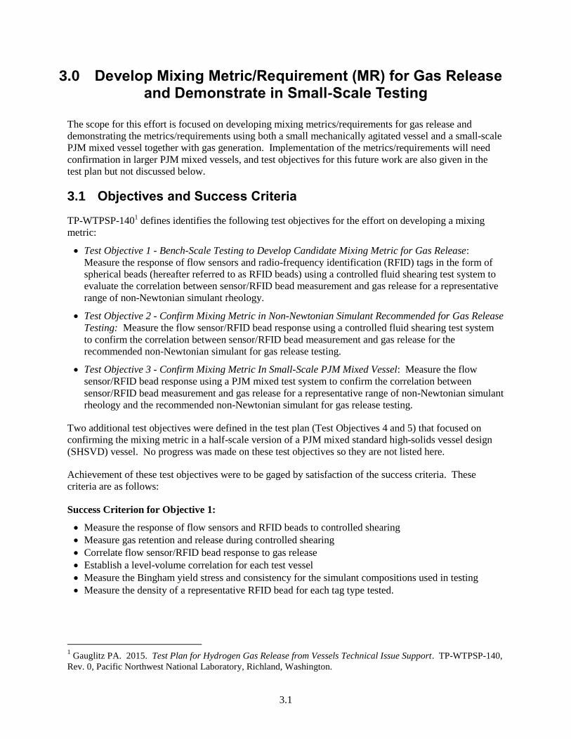
The scope for this effort is focused on developing mixing metrics/requirements for gas release and
demonstrating the metrics/requirements using both a small mechanically agitated vessel and a small-scale
PJM mixed vessel together with gas generation. Implementation of the metrics/requirements will need
confirmation in larger PJM mixed vessels, and test objectives for this future work are also given in the
test plan but not discussed below.
3.1 Objectives and Success Criteria
TP-WTPSP-1401 defines identifies the following test objectives for the effort on developing a mixing
metric:
Test Objective 1 - Bench-Scale Testing to Develop Candidate Mixing Metric for Gas Release:
Measure the response of flow sensors and radio-frequency identification (RFID) tags in the form of
spherical beads (hereafter referred to as RFID beads) using a controlled fluid shearing test system to
evaluate the correlation between sensor/RFID bead measurement and gas release for a representative
range of non-Newtonian simulant rheology.
Test Objective 2 - Confirm Mixing Metric in Non-Newtonian Simulant Recommended for Gas Release
Testing: Measure the flow sensor/RFID bead response using a controlled fluid shearing test system
to confirm the correlation between sensor/RFID bead measurement and gas release for the
recommended non-Newtonian simulant for gas release testing.
Test Objective 3 - Confirm Mixing Metric In Small-Scale PJM Mixed Vessel: Measure the flow
sensor/RFID bead response using a PJM mixed test system to confirm the correlation between
sensor/RFID bead measurement and gas release for a representative range of non-Newtonian simulant
rheology and the recommended non-Newtonian simulant for gas release testing.
Two additional test objectives were defined in the test plan (Test Objectives 4 and 5) that focused on
confirming the mixing metric in a half-scale version of a PJM mixed standard high-solids vessel design
(SHSVD) vessel. No progress was made on these test objectives so they are not listed here.
Achievement of these test objectives were to be gaged by satisfaction of the success criteria. These
criteria are as follows:
Success Criterion for Objective 1:
Measure the response of flow sensors and RFID beads to controlled shearing
Measure gas retention and release during controlled shearing
Correlate flow sensor/RFID bead response to gas release
Establish a level-volume correlation for each test vessel
Measure the Bingham yield stress and consistency for the simulant compositions used in testing
Measure the density of a representative RFID bead for each tag type tested.
1 Gauglitz PA. 2015. Test Plan for Hydrogen Gas Release from Vessels Technical Issue Support. TP-WTPSP-140,
Rev. 0, Pacific Northwest National Laboratory, Richland, Washington.
3.2
Success Criterion for Objective 2:
Measure the response of flow sensors and RFID beads to controlled shearing
Measure gas retention and release during controlled shearing
Confirm correlation of flow sensor/RFID bead response to gas release
Measure the Bingham yield stress and consistency for the simulant compositions used in testing
Measure density of representative RFID bead for each tag type tested.
Success Criterion for Objective 3:
Measure the response of flow sensors and RFID beads in a small-scale PJM mixed vessel
Measure gas retention and release during PJM mixing
Confirm correlation of flow sensor/RFID bead response to gas release
Establish a level-volume correlation for test vessel
Measure the Bingham yield stress and consistency for the simulant compositions used in testing
Measure density of representative RFID bead for each tag type tested
Quantify degradation of RFID beads during PJM operation.
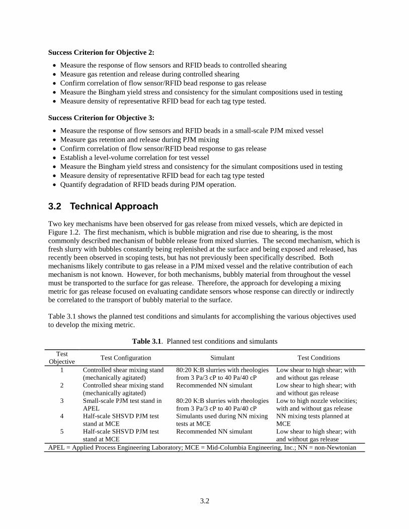
3.2 Technical Approach
Two key mechanisms have been observed for gas release from mixed vessels, which are depicted in
Figure 1.2. The first mechanism, which is bubble migration and rise due to shearing, is the most
commonly described mechanism of bubble release from mixed slurries. The second mechanism, which is
fresh slurry with bubbles constantly being replenished at the surface and being exposed and released, has
recently been observed in scoping tests, but has not previously been specifically described. Both
mechanisms likely contribute to gas release in a PJM mixed vessel and the relative contribution of each
mechanism is not known. However, for both mechanisms, bubbly material from throughout the vessel
must be transported to the surface for gas release. Therefore, the approach for developing a mixing
metric for gas release focused on evaluating candidate sensors whose response can directly or indirectly
be correlated to the transport of bubbly material to the surface.
Table 3.1 shows the planned test conditions and simulants for accomplishing the various objectives used
to develop the mixing metric.
Table 3.1. Planned test conditions and simulants
Test
Objective Test Configuration Simulant Test Conditions
1 Controlled shear mixing stand
(mechanically agitated)
80:20 K:B slurries with rheologies
from 3 Pa/3 cP to 40 Pa/40 cP
Low shear to high shear; with
and without gas release
2 Controlled shear mixing stand
(mechanically agitated)
Recommended NN simulant Low shear to high shear; with
and without gas release
3 Small-scale PJM test stand in
APEL
80:20 K:B slurries with rheologies
from 3 Pa/3 cP to 40 Pa/40 cP
Low to high nozzle velocities;
with and without gas release
4 Half-scale SHSVD PJM test
stand at MCE
Simulants used during NN mixing
tests at MCE
NN mixing tests planned at
MCE
5 Half-scale SHSVD PJM test
stand at MCE
Recommended NN simulant Low shear to high shear; with
and without gas release
APEL = Applied Process Engineering Laboratory; MCE = Mid-Columbia Engineering, Inc.; NN = non-Newtonian

3.3
The initial step in developing a mixing metric for gas release is to evaluate candidate sensors in a test
system with controlled shearing. Figure 3.1 shows a conceptual apparatus for developing a mixing metric
for gas release where controlled shearing is applied to a non-Newtonian slurry simulant. Sensors (e.g.,
flow, shear, and RFID beads) will be evaluated at various conditions of shear and fluid rheological
properties to determine whether their response can be correlated to gas release. Testing will be done with
and without gas release. Although only a single simulant was used in the preliminary studies reported
here, the plan was to use a range of simulants including the simulant being developed for gas release
testing (Section 5.0).
Figure 3.1. Conceptual apparatus with controlled shearing for correlating bubble release with flow
sensor and RFID bead response
Once a mixing metric is developed, the performance of the metric was planned to be demonstrated with
gas release in a small-scale PJM mixed vessel. Figure 3.2 shows a conceptual PJM mixed vessel for
evaluating two flow sensors (Met-Flow UVP-DUO and Valeport Electromagnetic (EM) sensors), and the
RFID beads.
Preliminary scoping work was done on evaluating RFID beads and flow sensors to assess their
applicability to meeting the goals of Test Objectives 1 and 2. Specifically, two types of RFID beads were
evaluated and two types of flow sensors (Met-Flow Ultrasonic Velocity Profiler [UVP] and Valeport
Electro Magnetic) were tested. The following sections present the accomplishments to date. As
mentioned previously, all work was preliminary and not performed according to any approved test plans,
test procedures, or test instructions and is For Information Only (FIO).

3.4
Figure 3.2. Conceptual PJM mixed vessel for correlating bubble release with flow sensor and RFID bead
response
3.3 RFID Tag Development
The driver behind using RFID beads for gas release testing is that their size and density can be tuned to
provide direct indication of the transport of gas bubbles to the surface. Because of the size limitation of
the RFID beads (typically no smaller than ~ 9 mm), the density of the tags was the key variable
manipulated to represent the rise velocities of ~3 mm gas bubbles (assumed bubble size) through a ~30 Pa
non-Newtonian fluids, provided that the material is sheared sufficiently to allow bubbles to rise. This
section presents the approach used to produce RFID embedded beads of different tag types and bead
densities. This section also presents the quantities of the various components required for implementation
of RFID beads in the 16 ft vessel. The evaluation of RFID beads is presented in Section 3.5.
3.3.1 Types of RFID Beads
RFID beads can either be active or passive. Active RFID beads contain an internal battery enabling them
to actively transmit signals. They are generally larger than passive RFID beads because they require
space for an internal power source. Passive RFID beads do not have an internal power source; they
contain a microchip and an antenna. As the name implies, passive RFID beads do not actively transmit
radio-frequency signals. Instead, they are powered by the electromagnetic waves emitted by the reader as
they enter the reader’s interrogation zone. The microchip inside the tag activates upon detecting an
interrogating signal from the reader and transmits a signal. Due to their small tag size (~9 mm), passive
RFID beads were selected for this work.
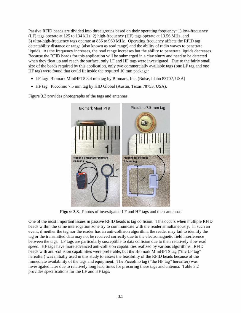
3.5
Passive RFID beads are divided into three groups based on their operating frequency: 1) low-frequency
(LF) tags operate at 125 to 134 kHz; 2) high-frequency (HF) tags operate at 13.56 MHz, and
3) ultra-high-frequency tags operate at 856 to 960 MHz. Operating frequency affects the RFID tag
detectability distance or range (also known as read range) and the ability of radio waves to penetrate
liquids. As the frequency increases, the read range increases but the ability to penetrate liquids decreases.
Because the RFID beads for this application will be submerged in a clay slurry and need to be detected
when they float up and reach the surface, only LF and HF tags were investigated. Due to the fairly small
size of the beads required by this application, only two commercially available tags (one LF tag and one
HF tag) were found that could fit inside the required 10 mm package:
LF tag: Biomark MiniHPT8 8.4 mm tag by Biomark, Inc. (Boise, Idaho 83702, USA)
HF tag: Piccolino 7.5 mm tag by HID Global (Austin, Texas 78753, USA).
Figure 3.3 provides photographs of the tags and antennas.
Figure 3.3. Photos of investigated LF and HF tags and their antennas
One of the most important issues in passive RFID beads is tag collision. This occurs when multiple RFID
beads within the same interrogation zone try to communicate with the reader simultaneously. In such an
event, if neither the tag nor the reader has an anti-collision algorithm, the reader may fail to identify the
tag or the transmitted data may not be received correctly due to the electromagnetic field interference
between the tags. LF tags are particularly susceptible to data collision due to their relatively slow read
speed. HF tags have more advanced anti-collision capabilities realized by various algorithms. RFID
beads with anti-collision capabilities were preferable, but the Biomark MiniHPT8 tag (“the LF tag”
hereafter) was initially used in this study to assess the feasibility of the RFID beads because of the
immediate availability of the tags and equipment. The Piccolino tag (“the HF tag” hereafter) was
investigated later due to relatively long lead times for procuring these tags and antenna. Table 3.2
provides specifications for the LF and HF tags.
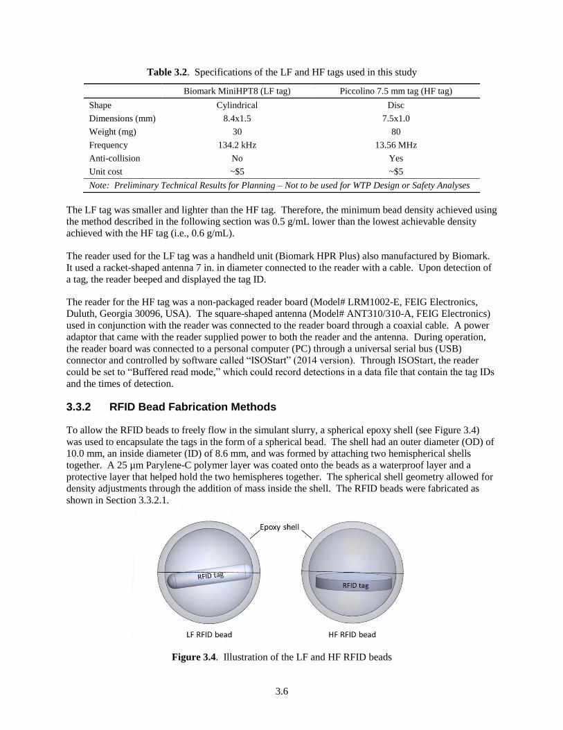
3.6
Table 3.2. Specifications of the LF and HF tags used in this study
Biomark MiniHPT8 (LF tag) Piccolino 7.5 mm tag (HF tag)
Shape Cylindrical Disc
Dimensions (mm) 8.4x1.5 7.5x1.0
Weight (mg) 30 80
Frequency 134.2 kHz 13.56 MHz
Anti-collision No Yes
Unit cost ~$5 ~$5
Note: Preliminary Technical Results for Planning – Not to be used for WTP Design or Safety Analyses
The LF tag was smaller and lighter than the HF tag. Therefore, the minimum bead density achieved using
the method described in the following section was 0.5 g/mL lower than the lowest achievable density
achieved with the HF tag (i.e., 0.6 g/mL).
The reader used for the LF tag was a handheld unit (Biomark HPR Plus) also manufactured by Biomark.
It used a racket-shaped antenna 7 in. in diameter connected to the reader with a cable. Upon detection of
a tag, the reader beeped and displayed the tag ID.
The reader for the HF tag was a non-packaged reader board (Model# LRM1002-E, FEIG Electronics,
Duluth, Georgia 30096, USA). The square-shaped antenna (Model# ANT310/310-A, FEIG Electronics)
used in conjunction with the reader was connected to the reader board through a coaxial cable. A power
adaptor that came with the reader supplied power to both the reader and the antenna. During operation,
the reader board was connected to a personal computer (PC) through a universal serial bus (USB)
connector and controlled by software called “ISOStart” (2014 version). Through ISOStart, the reader
could be set to “Buffered read mode,” which could record detections in a data file that contain the tag IDs
and the times of detection.
3.3.2 RFID Bead Fabrication Methods
To allow the RFID beads to freely flow in the simulant slurry, a spherical epoxy shell (see Figure 3.4)
was used to encapsulate the tags in the form of a spherical bead. The shell had an outer diameter (OD) of
10.0 mm, an inside diameter (ID) of 8.6 mm, and was formed by attaching two hemispherical shells
together. A 25 µm Parylene-C polymer layer was coated onto the beads as a waterproof layer and a
protective layer that helped hold the two hemispheres together. The spherical shell geometry allowed for
density adjustments through the addition of mass inside the shell. The RFID beads were fabricated as
shown in Section 3.3.2.1.
Figure 3.4. Illustration of the LF and HF RFID beads

3.7
3.3.2.1 Fabrication of the Hemispherical Shells
The hemispherical shells were fabricated using a silicone rubber mold (Figure 3.5). The mold consisted
of a top half (“Half A”) that had domes with a diameter of 8.6 mm and a bottom half (“Half B”) that had
hemispherical cavities with a diameter of 10.0 mm. The process used was:
1. The silicone mold was made from the XIAMETER® RTV-4230-E silicone rubber. Prior to use, a thin
layer of Dow-Corning 20 xylene solution (“DC20” hereafter; DC20:Xylene = 1:5 in weight) was
brushed onto all surfaces of the mold that would be in contact with the epoxy, as the release agent for
the epoxy.
2. The epoxy used was 3M Scotchcast Electrical Resin 5 (“3M epoxy” hereafter). This was a two-part
epoxy that required thorough mixing of the “Part A” and “Part B” at a 2:1 weight ratio prior to use.
After mixing the two parts, the epoxy was degassed in a vacuum oven for 10 minutes to eliminate
entrained air. The cavities in Half B of the mold were then filled with the degassed epoxy.
3. Half A was carefully lowered onto the bottom half with the domes aligned with the cavities. Four
alignment pins were used at the four corners of the mold to help the two halves stay aligned.
4. The mold was placed in an oven set to 160°F to cure the epoxy. During curing, a metal weight
(i.e., approximately 1 kg) was placed on top of the mold to eliminate any possible gap between the
two halves.
5. The mold was removed from the oven approximately 1 hour later. The hemispherical shells were
removed from the mold after the mold had been cooled to room temperature.
6. The hemispherical shells were then polished using a Dremel polish tool to remove the excess epoxy
hanging on the edge of the shell. The nominal weight of the hemispherical shell was 0.11 g.
Figure 3.5. Silicone rubber mold used for making RFID beads
3.3.2.2 Adjusting Bead Density
The specified densities of the final RFID beads were achieved by adding corresponding excess weight of
epoxy into the shell prior to gluing the two halves together. If the calculated amount of the excess epoxy
was more than what was needed to fill the hemispherical shell, the hemispherical shell became a solid
hemisphere. The solid hemispheres (either with or without the RFID tag inside) were made using the
Half B of the mold and an aluminum plate as the covering lid. Based on each target density,
combinations of five components were used to achieve the target weights for each target density as shown
in Table 3.3 for the HF tags. The target weights correspond to a 10.3 mm sphere, which is the equivalent
diameter that matches the estimated volume of the slightly non-spherical beads.
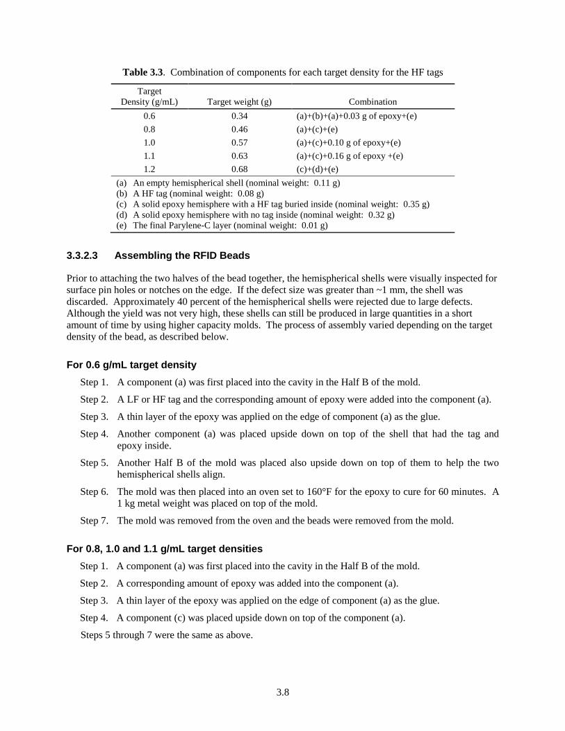
3.8
Table 3.3. Combination of components for each target density for the HF tags
Target
Density (g/mL) Target weight (g) Combination
0.6 0.34 (a)+(b)+(a)+0.03 g of epoxy+(e)
0.8 0.46 (a)+(c)+(e)
1.0 0.57 (a)+(c)+0.10 g of epoxy+(e)
1.1 0.63 (a)+(c)+0.16 g of epoxy +(e)
1.2 0.68 (c)+(d)+(e)
(a) An empty hemispherical shell (nominal weight: 0.11 g)
(b) A HF tag (nominal weight: 0.08 g)
(c) A solid epoxy hemisphere with a HF tag buried inside (nominal weight: 0.35 g)
(d) A solid epoxy hemisphere with no tag inside (nominal weight: 0.32 g)
(e) The final Parylene-C layer (nominal weight: 0.01 g)
3.3.2.3 Assembling the RFID Beads
Prior to attaching the two halves of the bead together, the hemispherical shells were visually inspected for
surface pin holes or notches on the edge. If the defect size was greater than ~1 mm, the shell was
discarded. Approximately 40 percent of the hemispherical shells were rejected due to large defects.
Although the yield was not very high, these shells can still be produced in large quantities in a short
amount of time by using higher capacity molds. The process of assembly varied depending on the target
density of the bead, as described below.
For 0.6 g/mL target density
Step 1. A component (a) was first placed into the cavity in the Half B of the mold.
Step 2. A LF or HF tag and the corresponding amount of epoxy were added into the component (a).
Step 3. A thin layer of the epoxy was applied on the edge of component (a) as the glue.
Step 4. Another component (a) was placed upside down on top of the shell that had the tag and
epoxy inside.
Step 5. Another Half B of the mold was placed also upside down on top of them to help the two
hemispherical shells align.
Step 6. The mold was then placed into an oven set to 160°F for the epoxy to cure for 60 minutes. A
1 kg metal weight was placed on top of the mold.
Step 7. The mold was removed from the oven and the beads were removed from the mold.
For 0.8, 1.0 and 1.1 g/mL target densities
Step 1. A component (a) was first placed into the cavity in the Half B of the mold.
Step 2. A corresponding amount of epoxy was added into the component (a).
Step 3. A thin layer of the epoxy was applied on the edge of component (a) as the glue.
Step 4. A component (c) was placed upside down on top of the component (a).
Steps 5 through 7 were the same as above.

3.9
For 1.2 g/mL target density
Step 1. A component (d) was first placed into the cavity in the Half B of the mold.
Step 2. A thin layer of epoxy was applied on the flat top surface of the component (d) as the glue.
Step 3. A component (c) was placed upside down on top of the component (d).
Step 4. No step 4.
Steps 5 through 7 were the same as above.
3.3.2.4 Pinhole Check Bead Patching
After the two hemispheres were attached, the beads were checked under a microscope for pinholes on the
surface and seam. When a small pinhole was found, scotch tape was used to cover the pinhole and a thin
layer of hot-melt glue was applied over the tape to keep it in place. It was determined that without the
tape, neither the epoxy nor hot-melt glue was effective at covering the pinholes. Their surface tension
tended to draw them into the bead when applied without the tape.
3.3.2.5 Parylene-C Waterproof Coating
After the beads were visually inspected for pinholes and patched (as necessary), they were coated with a
25 µm Parylene-C layer. Parylene-C is a waterproof polymer often used by industries for moisture
resistance. In this case, Parylene-C also served as a packaging layer to enclose the RFID beads and make
them less susceptible to cracking at the jointing edge.
3.3.3 RFID Bead Fabrication Results
Figure 3.6 is photograph of the RFID bead fabricated using the methods described previously. These
beads were found to have a 10.6 mm diameter (instead of 10.0 mm) in the direction normal to the planar
direction of the mold; most likely due to the manufacturing tolerance of the 3D printer used to fabricate
the mold. The bead diameter in the planar direction was 9.9 to 10.1 mm, much closer to the nominal
value. The 0.6 mm error in the diameter was taken into consideration when calculating the required tag
weight for each target density. The volume was calculated by considering the shape of the tag as a
combination of a perfect sphere (10.0 mm in diameter) and a circular disc (10.0 mm in diameter and
0.6 mm thick).
For RFID beads of a given target density, the variation in weight was found to be about ± 0.02 g, which
translated into a density uncertainty of 3 to 6 percent.
As a quality control step, the RFID beads were placed into a pressurized water tank at 2 atm (gauge) for
10 minutes. The 2 atm pressure was the estimated maximum pressure the beads would experience when
tested in the actual slurry vessel. The weights of the RFID beads were recorded before and after the test.
After the test, beads with a weight increase greater than 0.01 g were rejected. Experiments showed that
the beads were sufficiently durable to survive under that pressure. However, approximately 10 to 20
percent of the beads could fail this test due to small leaks that were too small to be detected during visual
inspection under a microscope.
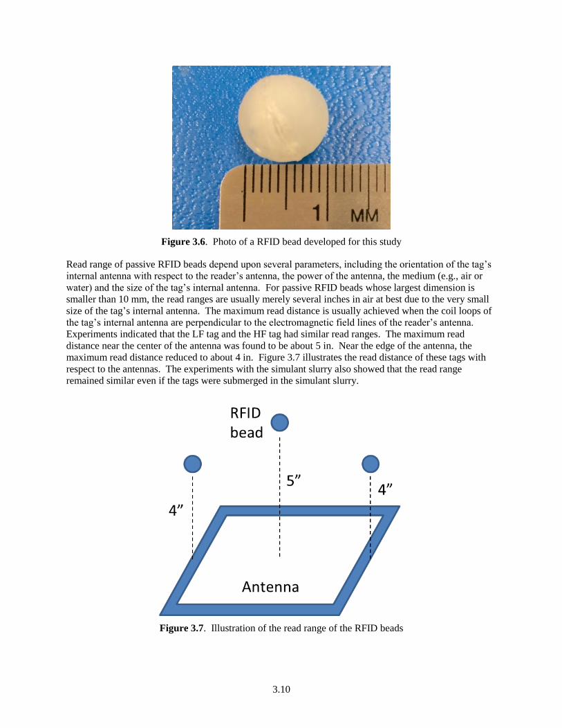
3.10
Figure 3.6. Photo of a RFID bead developed for this study
Read range of passive RFID beads depend upon several parameters, including the orientation of the tag’s
internal antenna with respect to the reader’s antenna, the power of the antenna, the medium (e.g., air or
water) and the size of the tag’s internal antenna. For passive RFID beads whose largest dimension is
smaller than 10 mm, the read ranges are usually merely several inches in air at best due to the very small
size of the tag’s internal antenna. The maximum read distance is usually achieved when the coil loops of
the tag’s internal antenna are perpendicular to the electromagnetic field lines of the reader’s antenna.
Experiments indicated that the LF tag and the HF tag had similar read ranges. The maximum read
distance near the center of the antenna was found to be about 5 in. Near the edge of the antenna, the
maximum read distance reduced to about 4 in. Figure 3.7 illustrates the read distance of these tags with
respect to the antennas. The experiments with the simulant slurry also showed that the read range
remained similar even if the tags were submerged in the simulant slurry.
Figure 3.7. Illustration of the read range of the RFID beads

3.11
Experiments using the both LF and HF beads were performed in a small 2 ft deep vessel. During the
experiments, the respective antennas were positioned approximately 3 in. above the surface of the slurry
with the planes of the antenna loops parallel to the slurry surface. Both types of RFID beads were
detected when they rose near the surface. HF bead detection was much more consistent than LF bead
detection, likely because the internal antenna in the LF tag was much smaller than that in the HF tag.
Another advantage of the HF tag found during the experiments was that the software (i.e., ISOStart 2014
Version) could display and record the detection of tags with the corresponding time stamp. This allowed
for recording the average time taken for a particular bead to finish a traveling cycle between the top and
bottom of the vessel.
Experiments confirmed that LF tags are more prone to tag collision than HF tags due to their slower read
speed. When two or more of the LF tags were placed in the proximity of the racket antenna of the HPR
Plus reader, in most cases, no tags were detected. Occasionally, one tag was still detected by the reader—
probably because the coil orientations of the other tags’ internal antennas, with respect to the reader’s
antenna, were less ideal compared to the one detected. Because of the severe tag collision issue, LF tags
are not recommended for this application.
The HF tags were much less susceptible to tag collision because of their anti-collision capability.
However, all RFID beads have signal collision issues to a certain degree when multiple RFID beads are
present in the read zone of a same antenna. In the case of HF tags, because of the much faster read speed
(tens of milliseconds per tag) compared to that of LF tags (~0.5 s), HF readers can implement a so-called
“anti-collision” algorithm to interrogate tags one at a time. When multiple HF tags respond to the same
reader, because this process happens so quickly, it would appear to the user as if they are all read at once.
Because all the tags still respond to the reader individually, all anti-collision algorithms still have a limit
of maximum number of tags that can be detected “simultaneously.” This was also observed in these
experiments. Under ideal conditions (i.e., all the tags sitting stationary on a bench-top with their internal
antenna loops parallel to the antenna loop of the reader) the LRM1002-E reader was able to detect, at
most, about 40 tags “simultaneously.” This maximum number of detected tags was limited by the
anti-collision algorithm built into the tags and the processing capability of the microchip in the reader.
When the tags are in motion, which is the case for this RFID bead application, anti-collision algorithms
function less effectively. As described in Section 3.3.1, a passive RFID tag is energized through the
electromagnetic field of the reader’s antenna. The energy it receives is determined by 1) the distance
between the tag and the reader’s antenna and 2) the relative orientation of the tag’s internal antenna with
respect to the reader’s antenna. In this application, because of the very small size of the internal antenna,
the amount of energy the tag received was fairly sensitive to those two parameters. The electromagnetic
field lines of a reader’s antenna are illustrated in Figure 3.8. As a tag moves across the antenna field,
either one or both of those two parameters are constantly changing, which increase the time needed for
the reader to identify the tag. If the tag is near the boundary of the maximum read range, at certain
locations, it may not receive sufficient energy to reply back to the reader. As a result, depending on the
velocity at which the tags are moving, the maximum number of the tags that can be detected is smaller
than in the case of stationary tags. Preliminary experiments for this situation were performed in the lab
by letting the HF RFID beads free fall through the antenna loop of the ANT310/310-A antenna. The tag
velocity was converted from the vertical distance between the antenna and initial position of the tags. It
was found that at a velocity of 4 to 8 ft/s, the maximum number of tags detected was eight. Evidently, at
a given velocity, the number of tags detected is inconsistent due to the random nature of the orientation of
each tag’s internal antenna.
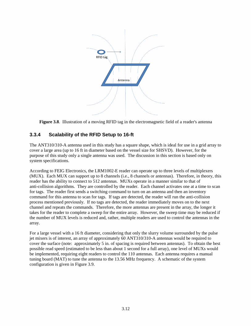
3.12
Figure 3.8. Illustration of a moving RFID tag in the electromagnetic field of a reader's antenna
3.3.4 Scalability of the RFID Setup to 16-ft
The ANT310/310-A antenna used in this study has a square shape, which is ideal for use in a grid array to
cover a large area (up to 16 ft in diameter based on the vessel size for SHSVD). However, for the
purpose of this study only a single antenna was used. The discussion in this section is based only on
system specifications.
According to FEIG Electronics, the LRM1002-E reader can operate up to three levels of multiplexers
(MUX). Each MUX can support up to 8 channels (i.e., 8 channels or antennas). Therefore, in theory, this
reader has the ability to connect to 512 antennas. MUXs operate in a manner similar to that of
anti-collision algorithms. They are controlled by the reader. Each channel activates one at a time to scan
for tags. The reader first sends a switching command to turn on an antenna and then an inventory
command for this antenna to scan for tags. If tags are detected, the reader will run the anti-collision
process mentioned previously. If no tags are detected, the reader immediately moves on to the next
channel and repeats the commands. Therefore, the more antennas are present in the array, the longer it
takes for the reader to complete a sweep for the entire array. However, the sweep time may be reduced if
the number of MUX levels is reduced and, rather, multiple readers are used to control the antennas in the
array.
For a large vessel with a 16 ft diameter, considering that only the slurry volume surrounded by the pulse
jet mixers is of interest, an array of approximately 60 ANT310/310-A antennas would be required to
cover the surface (note: approximately 5 in. of spacing is required between antennas). To obtain the best
possible read speed (estimated to be less than about 1 second for a full array), one level of MUXs would
be implemented, requiring eight readers to control the 110 antennas. Each antenna requires a manual
tuning board (MAT) to tune the antenna to the 13.56 MHz frequency. A schematic of the system
configuration is given in Figure 3.9.
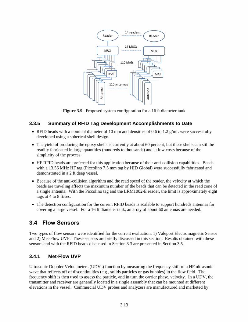
3.13
Figure 3.9. Proposed system configuration for a 16 ft diameter tank
3.3.5 Summary of RFID Tag Development Accomplishments to Date
RFID beads with a nominal diameter of 10 mm and densities of 0.6 to 1.2 g/mL were successfully
developed using a spherical shell design.
The yield of producing the epoxy shells is currently at about 60 percent, but these shells can still be
readily fabricated in large quantities (hundreds to thousands) and at low costs because of the
simplicity of the process.
HF RFID beads are preferred for this application because of their anti-collision capabilities. Beads
with a 13.56 MHz HF tag (Piccolino 7.5 mm tag by HID Global) were successfully fabricated and
demonstrated in a 2 ft deep vessel.
Because of the anti-collision algorithm and the read speed of the reader, the velocity at which the
beads are traveling affects the maximum number of the beads that can be detected in the read zone of
a single antenna. With the Piccolino tag and the LRM1002-E reader, the limit is approximately eight
tags at 4 to 8 ft/sec.
The detection configuration for the current RFID beads is scalable to support hundreds antennas for
covering a large vessel. For a 16 ft diameter tank, an array of about 60 antennas are needed.
3.4 Flow Sensors
Two types of flow sensors were identified for the current evaluation: 1) Valeport Electromagnetic Sensor
and 2) Met-Flow UVP. These sensors are briefly discussed in this section. Results obtained with these
sensors and with the RFID beads discussed in Section 3.3 are presented in Section 3.5.
3.4.1 Met-Flow UVP
Ultrasonic Doppler Velocimeters (UDVs) function by measuring the frequency shift of a HF ultrasonic
wave that reflects off of discontinuities (e.g., solids particles or gas bubbles) in the flow field. The
frequency shift is then used to assess the particle, and in turn the carrier phase, velocity. In a UDV, the
transmitter and receiver are generally located in a single assembly that can be mounted at different
elevations in the vessel. Commercial UDV probes and analyzers are manufactured and marketed by
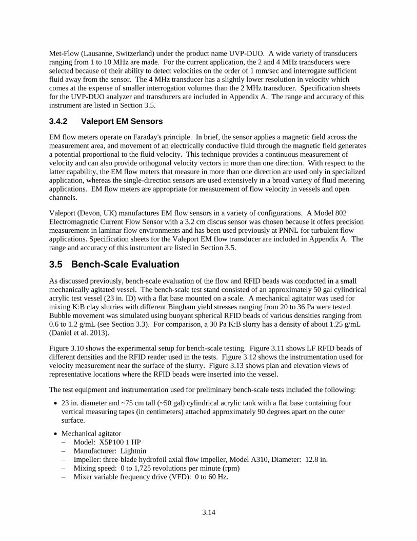
3.14
Met-Flow (Lausanne, Switzerland) under the product name UVP-DUO. A wide variety of transducers
ranging from 1 to 10 MHz are made. For the current application, the 2 and 4 MHz transducers were
selected because of their ability to detect velocities on the order of 1 mm/sec and interrogate sufficient
fluid away from the sensor. The 4 MHz transducer has a slightly lower resolution in velocity which
comes at the expense of smaller interrogation volumes than the 2 MHz transducer. Specification sheets
for the UVP-DUO analyzer and transducers are included in Appendix A. The range and accuracy of this
instrument are listed in Section 3.5.
3.4.2 Valeport EM Sensors
EM flow meters operate on Faraday's principle. In brief, the sensor applies a magnetic field across the
measurement area, and movement of an electrically conductive fluid through the magnetic field generates
a potential proportional to the fluid velocity. This technique provides a continuous measurement of
velocity and can also provide orthogonal velocity vectors in more than one direction. With respect to the
latter capability, the EM flow meters that measure in more than one direction are used only in specialized
application, whereas the single-direction sensors are used extensively in a broad variety of fluid metering
applications. EM flow meters are appropriate for measurement of flow velocity in vessels and open
channels.
Valeport (Devon, UK) manufactures EM flow sensors in a variety of configurations. A Model 802
Electromagnetic Current Flow Sensor with a 3.2 cm discus sensor was chosen because it offers precision
measurement in laminar flow environments and has been used previously at PNNL for turbulent flow
applications. Specification sheets for the Valeport EM flow transducer are included in Appendix A. The
range and accuracy of this instrument are listed in Section 3.5.
3.5 Bench-Scale Evaluation
As discussed previously, bench-scale evaluation of the flow and RFID beads was conducted in a small
mechanically agitated vessel. The bench-scale test stand consisted of an approximately 50 gal cylindrical
acrylic test vessel (23 in. ID) with a flat base mounted on a scale. A mechanical agitator was used for
mixing K:B clay slurries with different Bingham yield stresses ranging from 20 to 36 Pa were tested.
Bubble movement was simulated using buoyant spherical RFID beads of various densities ranging from
0.6 to 1.2 g/mL (see Section 3.3). For comparison, a 30 Pa K:B slurry has a density of about 1.25 g/mL
(Daniel et al. 2013).
Figure 3.10 shows the experimental setup for bench-scale testing. Figure 3.11 shows LF RFID beads of
different densities and the RFID reader used in the tests. Figure 3.12 shows the instrumentation used for
velocity measurement near the surface of the slurry. Figure 3.13 shows plan and elevation views of
representative locations where the RFID beads were inserted into the vessel.
The test equipment and instrumentation used for preliminary bench-scale tests included the following:
23 in. diameter and ~75 cm tall (~50 gal) cylindrical acrylic tank with a flat base containing four
vertical measuring tapes (in centimeters) attached approximately 90 degrees apart on the outer
surface.
Mechanical agitator
– Model: X5P100 1 HP
– Manufacturer: Lightnin
– Impeller: three-blade hydrofoil axial flow impeller, Model A310, Diameter: 12.8 in.
– Mixing speed: 0 to 1,725 revolutions per minute (rpm)
– Mixer variable frequency drive (VFD): 0 to 60 Hz.
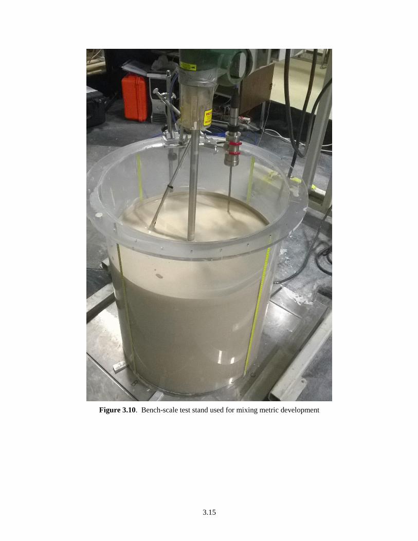
3.15
Figure 3.10. Bench-scale test stand used for mixing metric development
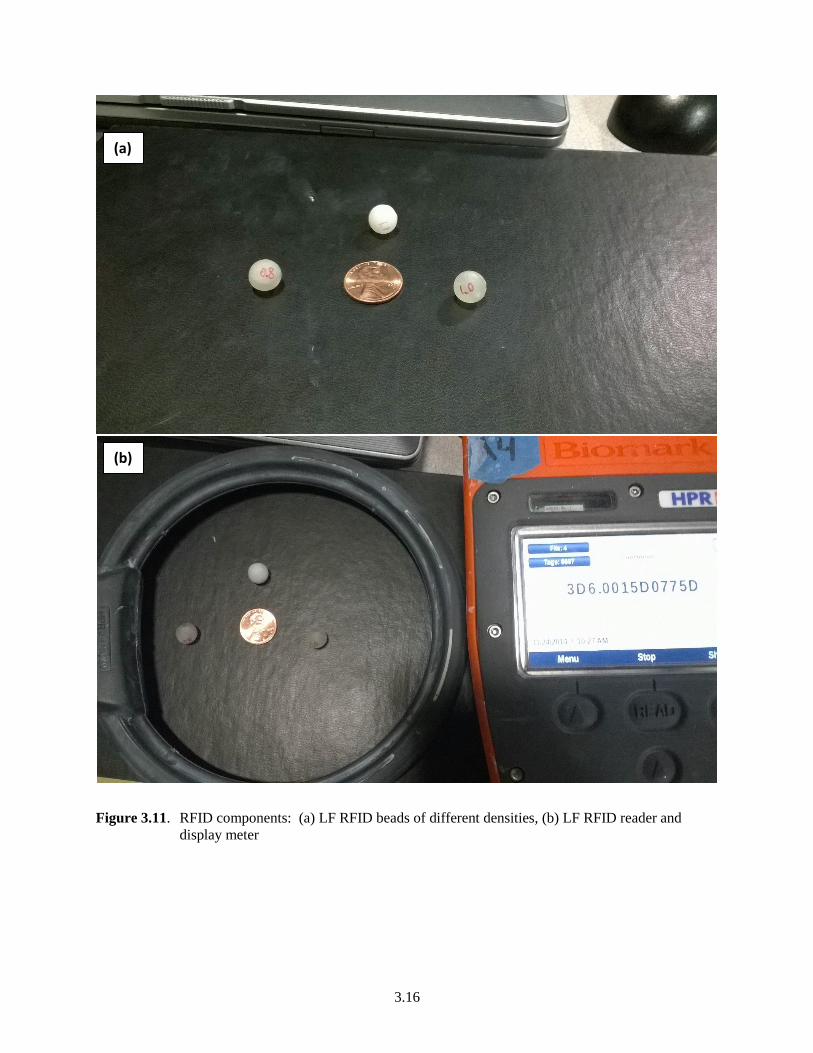
3.16
Figure 3.11. RFID components: (a) LF RFID beads of different densities, (b) LF RFID reader and
display meter
(a)
(b)
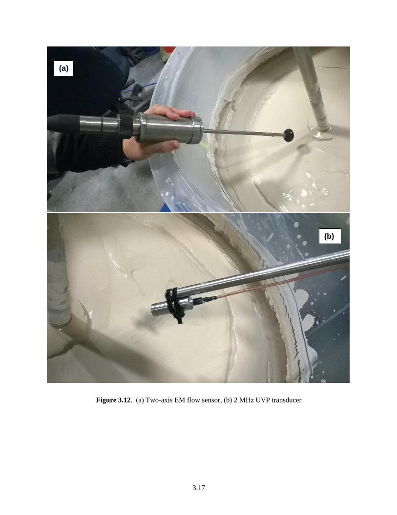
3.17
Figure 3.12. (a) Two-axis EM flow sensor, (b) 2 MHz UVP transducer
(a)
(b)
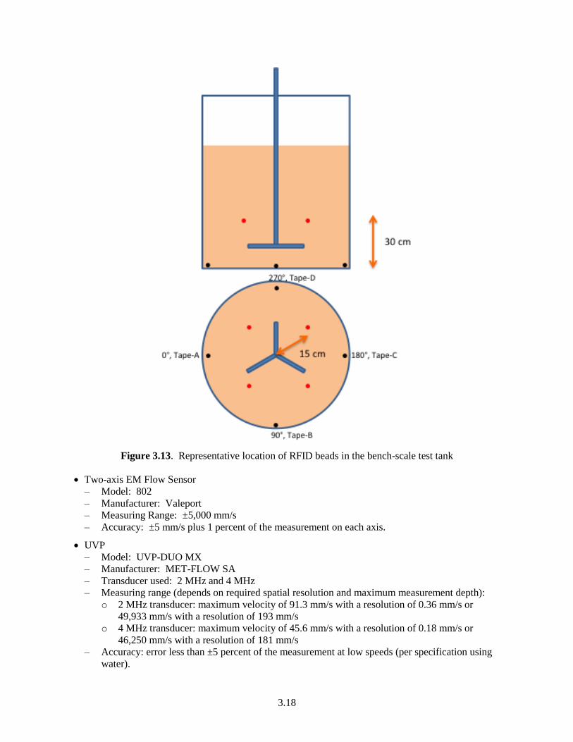
3.18
Figure 3.13. Representative location of RFID beads in the bench-scale test tank
Two-axis EM Flow Sensor
– Model: 802
– Manufacturer: Valeport
– Measuring Range: ±5,000 mm/s
– Accuracy: ±5 mm/s plus 1 percent of the measurement on each axis.
UVP
– Model: UVP-DUO MX
– Manufacturer: MET-FLOW SA
– Transducer used: 2 MHz and 4 MHz
– Measuring range (depends on required spatial resolution and maximum measurement depth):
o 2 MHz transducer: maximum velocity of 91.3 mm/s with a resolution of 0.36 mm/s or
49,933 mm/s with a resolution of 193 mm/s
o 4 MHz transducer: maximum velocity of 45.6 mm/s with a resolution of 0.18 mm/s or
46,250 mm/s with a resolution of 181 mm/s
– Accuracy: error less than ±5 percent of the measurement at low speeds (per specification using
water).

3.19
RFID beads (using LF and HF RFID beads) of different densities (0.6 to 1.2 g/mL).
RFID readers to detect the LF and HF tags that reach the slurry surface.
3.5.1 Shakedown Tests
A few shakedown tests were conducted to determine whether surface motion during gas release
corresponds to RFID tag release, velocity instrument sensitivities for measuring flow, and the adequacy of
operational procedure. Several key observations from the shakedown tests enabled refinement of the test
procedure for later tests. These shakedown tests are discussed below.
3.5.1.1 Shakedown Test 1 – Using RFID Beads a Surrogate Gas Bubbles
The first shakedown test was conducted using ~32 wt%, 80:20 K:B clay of ~20 Pa Bingham yield stress
using the test stand discussed previously (see Figure 3.10). During this test, the mechanical agitator was
arranged such that the impeller was approximately 6 in. above the bottom of the tank. The slurry was
prepared in a separate vessel and transferred into the test tank until the level was approximately 6 in.
above the top of the impeller. At this point, four RFID beads with a density of approximately 0.6 g/mL
were placed at a radial position of about 15 cm (on surface) and the remaining slurry from the drum was
pumped into the test tank. The elevation of these tags was approximately 30 cm above the vessel floor.
The final level of the tank was approximately 52 cm from the vessel floor. A surface scan after all the
slurry was transferred to the test vessel indicated that the tags managed to rise to the surface as the slurry
was being pumped into the vessel. The tags were manually inserted back in to the tank at 30 cm from the
vessel floor. Later tests used a long-handled sieve to insert RFID beads in the tank at a desired level.
The test was started with a mixing speed of 5 Hz (144 rpm), and was later increased to 15 Hz (431 rpm)
and then to 30 Hz (862 rpm). The slurry was mixed for 15 minutes at each mixing speed and the surface
was frequently scanned for the beads during mixing. The agitator was stopped before each speed change.
No tags were detected until the mixing speed was >30 Hz. When the agitator was stopped and started at
45 Hz (1,294 rpm) all four tags were detected at the surface within 1 minute of mixing. This narrowed
the mixing speed for gas release (i.e., tag rise) to the 30 to 45 Hz range for the slurry used.
The run was repeated after reinserting all the four tags at 30 cm level (e.g., ≈12 in. from the bottom) and
starting the mixing at 33 Hz (949 rpm). After 10 minutes, the mixing speed was increased to 34 Hz and
then, after 10 more minutes, to 35 Hz (1,006 rpm). At this speed all four tags were detected at the surface
within 2 to 3 minutes of mixing.
3.5.1.2 Shakedown Test 2: With Hydrogen Peroxide Addition
To assess how the release of tags with the mixer speeds identified in Shakedown Test 1 corresponds to
actual gas release, Shakedown Test 2, a mixing test using the test material from Test 1 with hydrogen
peroxide (H2O2) injection, was conducted. The test was started with mixing the slurry at a high speed
(50 Hz [1,437 rpm]) for nearly 2 hours. After approximately 2 hours, the mixer was stopped and slurry
samples were collected for rheology characterization. Mixing was restarted at 40 Hz (1,150 rpm) and
approximately 1 L of 3 percent peroxide solution was added to the slurry while mixing. The amount of
peroxide added resulted in approximately 0.1 wt% H2O2 in the batch. Significant gas bubble generation
(O2) was observed during the blending of the peroxide and the slurry. After 15 minutes, the mixer was
stopped and eight RFID beads of ~0.6 g/mL density were inserted in to the slurry: four tags at the bottom
corner (i.e., near the tapes shown in Figure 3.13) and four tags nearly 6 in. above the agitator at the tank’s
mid-radius. While waiting for sufficient gas to build up in the vessel without mixing, all eight tags were
detected at the surface. It was unclear if peroxide-generated bubbles rising to the surface assisted the

3.20
RFID beads in finding a sheared path for rising to the surface or if other mechanisms, such as bubble
growth and attachment on the tag surface (resulting in increased buoyancy) assisted the tags to rise. Thus,
the speed test was not conducted with active peroxide in the tank, as it would be unclear whether shearing
due to the release of the gas bubbles or due to mixing caused the tags to rise. For the same
aforementioned reason, tests with peroxide addition were not planned for later tests until the release of the
RFID beads of different densities due to mixer speed was first established.
3.5.1.3 Shakedown Tests 3-7: With RFID Beads of Various Densities
The clay slurry used in the peroxide shakedown test above was used later for Shakedown Tests 3 through
7 in which RFID beads of densities of approximately 0.6, 0.8, 1.0, and 1.1 g/mL, respectively, were
tested. Peroxide added in shakedown test 2 (see Section 3.5.1.2) diluted the slurry and reduced the
rheology of the simulant, and the simulant Bingham yield stress during tests 3-7 was ~15 Pa. In addition
to finding the optimal mixing velocity at which the tags rise to the surface, these tests also focused on
identification of issues with the procedure for final bench-scale tests. Each test was conducted using four
tags of a specific density placed at about midway between the wall and the agitator shaft at a level nearly
6 in. above the agitator. Later, the test was repeated with the same tags placed at the bottom corner of the
tank near tapes A, B, C, and D shown in Figure 3.10. Visual observations from tank walls indicated
limited or no motion of slurry in the top half of the vessel near the walls. Hence, it was decided that
future experiments should use tags at these locations. Table 3.4 summarizes the results from Shakedown
Tests 3 through 7. Table 3.4 shows that RFID beads, irrespective of their density and placement location,
rose to the surface at about 33 Hz (949 rpm) mixing speed. This is of significance because it indicates for
the range of tags, and hence bubble rise-velocities studied, gas bubbles would release irrespective of their
rise velocity (or size). Moreover, in such a scenario, the optimal mixing speed (shear or flow) needs to be
correlated with only the Bingham yield stress of the slurries as the tag densities did not show major
influence on the mixing speed at which tags rise to the surface. Note: care should be taken extrapolating
this result to bubbles with much smaller rise velocities than those investigated with the RFID beads.
Table 3.4. Summary of results from shakedown tests 3 to 7 using tags of 0.6, 0.8, 1.0 and 1.1 densities
Tags Placement
Location
Mixing speed in Hz (rpm)(b)
at which RFID beads floated to the surface
8(a)
tags of
0.6 g/mL
4 tags of
0.8 g/mL
4 tags of
1.0 g/mL
4 Tags of
1.1 g/mL
4 tags of 0.6
g/mL (Repeat)
6 in. above agitator 30 (862)
33 (949) 33 (949) 32.5(934) -
At bottom corners 33 (949) 33 (949) 33 (949) 33 (949)
(a) Four tags above agitator at midway between the wall and the agitator shaft and four at the bottom corners
near tapes A, B, C, and D shown in Figure 3.13.
(b) 1 Hz = 28.75 rpm
Note: Preliminary Technical Results for Planning – Not to be used for WTP Design or Safety Analyses
3.5.1.4 Observations and Notes from Shakedown Tests
Several observations were made regarding tag behavior and the experimental procedure during these
shakedown tests.
Often the tags inserted in the slurry (using a long-handled sieve) showed up at the surface right after
the placement via the shear path created while withdrawing the sieve. It is necessary to wait for some
time after tags insertion before starting the mixer.
The number of tags inserted appeared to influence the mixing speed at which tags rose to the surface
and the slurry’s surface motion. When more tags were inserted, surface motion seemed to occur at

3.21
lower velocities. To minimize this effect in the later tests with various tag densities, the same number
of tags (when available) were used at similar locations in the tank.
In some cases the tags broke into two hemispherical shells where they were bonded and never showed
up at the surface as the antennas inside are not buoyant.
The LF RFID scanner has a small detection range (i.e., within the 5 in. diameter shown in Figure 3.7).
Hence frequent visual surface scanning was necessary. There was a significant chance that tags could
rise in different, un-scanned locations.
A 1 to 2 in.-thick foam layer of slurry always appeared at the surface while mixing for more than
1 hour (this occurred both with and without gas generation by H2O2 decomposition). This stagnant
layer at the surface affected the recording ability of instruments (e.g., two-axis EM meter as it
measured flow past the sensor). It was unclear if this layer was low-density slurry with bubbles
(foam) or low-density particles in the K:B slurry rising to the surface.
The tags were often detected at the surface whenever the surface motion was just enough to shear and
break the foamy layer formed at the surface.
Estimation of starting speed of the agitator was necessary for reducing the testing duration. The
starting speeds were estimated prior to the tests by changing the mixing speed until slight surface
motion appeared.
The test using eight 0.6 g/mL density tags resulted in lower mixing speed for release (30 Hz
[862 rpm]) compared to other tests using four tags where the tags, irrespective of density, surfaced at
33 Hz (949 rpm). It was unclear if the shear paths created during the insertion of tags using a long-
handled sieve influenced the results.
Clay was observed to behave differently at a particular mixing speed. Sometimes the surface mixed
and rotated at 32 Hz (920 rpm) and other times the surface remained still at 33 Hz (949 rpm). This
could be a result of break time (i.e., no mixing) between the tags insertion and the beginning of tests.
Later tests were conducted with a break time of 1 hour.
3.5.2 Flow Instrument Tests
The work conducted during the shakedown phase also evaluated the Valeport Series 800 two-axis EM
(Model 802) and the Met-Flow UVP-DUO flow sensors. While both the instruments have reasonable
resolution to capture surface velocities corresponding to tag rise, a few issues were encountered while
using the Valeport EM velocity probe.
3.5.2.1 Valeport EM Flow Sensor
Model 802 uses Faraday principle to measure the flow past the sensor in two orthogonal axes. The
magnetic field is generated within the sensors by a coil, and the electronics detect the signal generated
across two pairs of electrodes for velocity components along the two axes. Model 802 has
user-configurable data acquisition rates of 1, 2, 4, 8, or 16 Hz of which 4 Hz recording was chosen for
testing.
During testing, Model 802 (shown in Figure 3.12a) was clamped to the side wall of the tank such that the
probe was vertical and the sensing portion of the probe was immersed to a depth of 1 to 2 in. from the
slurry surface. The sensor y-axis, indicated by a painted red dot, was pointed toward the center of the
tank (i.e., toward agitator’s shaft). In this configuration the y-velocity indicates flow in radial direction
and x-velocity indicates the flow in circumferential direction. Because the flow into the sensor is
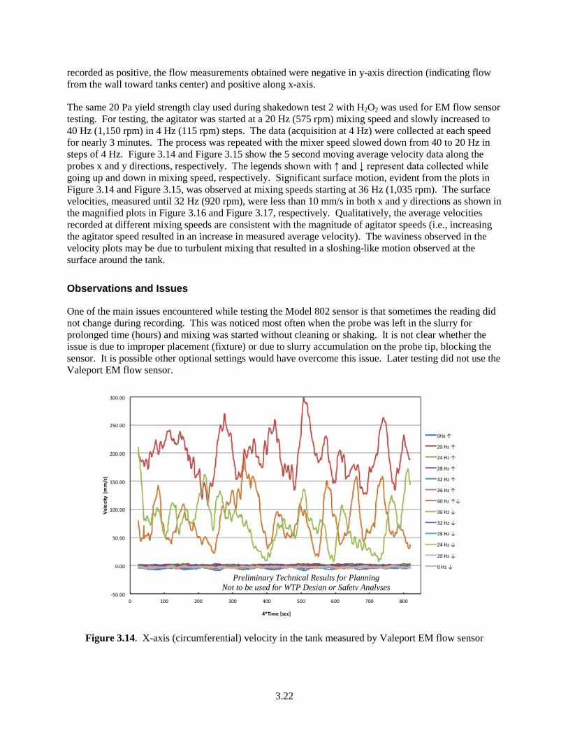
3.22
recorded as positive, the flow measurements obtained were negative in y-axis direction (indicating flow
from the wall toward tanks center) and positive along x-axis.
The same 20 Pa yield strength clay used during shakedown test 2 with H2O2 was used for EM flow sensor
testing. For testing, the agitator was started at a 20 Hz (575 rpm) mixing speed and slowly increased to
40 Hz (1,150 rpm) in 4 Hz (115 rpm) steps. The data (acquisition at 4 Hz) were collected at each speed
for nearly 3 minutes. The process was repeated with the mixer speed slowed down from 40 to 20 Hz in
steps of 4 Hz. Figure 3.14 and Figure 3.15 show the 5 second moving average velocity data along the
probes x and y directions, respectively. The legends shown with ↑ and ↓ represent data collected while
going up and down in mixing speed, respectively. Significant surface motion, evident from the plots in
Figure 3.14 and Figure 3.15, was observed at mixing speeds starting at 36 Hz (1,035 rpm). The surface
velocities, measured until 32 Hz (920 rpm), were less than 10 mm/s in both x and y directions as shown in
the magnified plots in Figure 3.16 and Figure 3.17, respectively. Qualitatively, the average velocities
recorded at different mixing speeds are consistent with the magnitude of agitator speeds (i.e., increasing
the agitator speed resulted in an increase in measured average velocity). The waviness observed in the
velocity plots may be due to turbulent mixing that resulted in a sloshing-like motion observed at the
surface around the tank.
Observations and Issues
One of the main issues encountered while testing the Model 802 sensor is that sometimes the reading did
not change during recording. This was noticed most often when the probe was left in the slurry for
prolonged time (hours) and mixing was started without cleaning or shaking. It is not clear whether the
issue is due to improper placement (fixture) or due to slurry accumulation on the probe tip, blocking the
sensor. It is possible other optional settings would have overcome this issue. Later testing did not use the
Valeport EM flow sensor.
Figure 3.14. X-axis (circumferential) velocity in the tank measured by Valeport EM flow sensor
Preliminary Technical Results for Planning
Not to be used for WTP Design or Safety Analyses

3.23
Figure 3.15. Y-axis (radial) velocity in the tank measured by Valeport EM flow sensor
Figure 3.16. Magnified x-axis (circumferential) velocity in the tank measured by Valeport EM flow
sensor (zoomed in view of Figure 3.14)
Preliminary Technical Results for Planning
Not to be used for WTP Design or Safety Analyses
Preliminary Technical Results for Planning
Not to be used for WTP Design or Safety Analyses
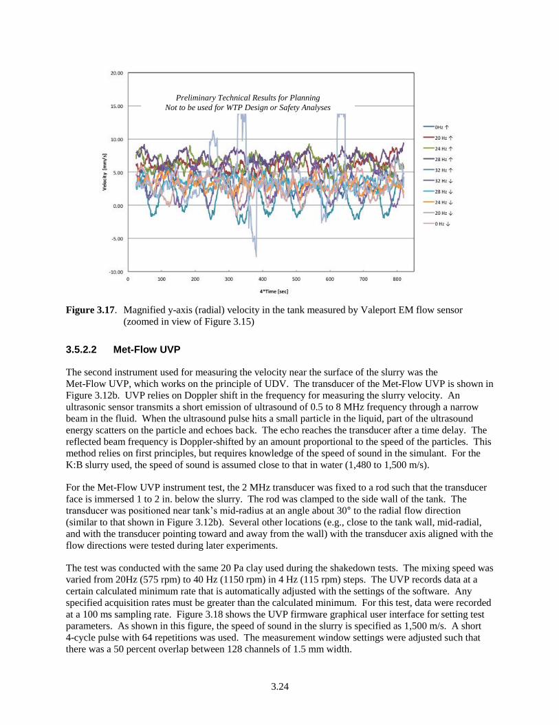
3.24
Figure 3.17. Magnified y-axis (radial) velocity in the tank measured by Valeport EM flow sensor
(zoomed in view of Figure 3.15)
3.5.2.2 Met-Flow UVP
The second instrument used for measuring the velocity near the surface of the slurry was the
Met-Flow UVP, which works on the principle of UDV. The transducer of the Met-Flow UVP is shown in
Figure 3.12b. UVP relies on Doppler shift in the frequency for measuring the slurry velocity. An
ultrasonic sensor transmits a short emission of ultrasound of 0.5 to 8 MHz frequency through a narrow
beam in the fluid. When the ultrasound pulse hits a small particle in the liquid, part of the ultrasound
energy scatters on the particle and echoes back. The echo reaches the transducer after a time delay. The
reflected beam frequency is Doppler-shifted by an amount proportional to the speed of the particles. This
method relies on first principles, but requires knowledge of the speed of sound in the simulant. For the
K:B slurry used, the speed of sound is assumed close to that in water (1,480 to 1,500 m/s).
For the Met-Flow UVP instrument test, the 2 MHz transducer was fixed to a rod such that the transducer
face is immersed 1 to 2 in. below the slurry. The rod was clamped to the side wall of the tank. The
transducer was positioned near tank’s mid-radius at an angle about 30° to the radial flow direction
(similar to that shown in Figure 3.12b). Several other locations (e.g., close to the tank wall, mid-radial,
and with the transducer pointing toward and away from the wall) with the transducer axis aligned with the
flow directions were tested during later experiments.
The test was conducted with the same 20 Pa clay used during the shakedown tests. The mixing speed was
varied from 20Hz (575 rpm) to 40 Hz (1150 rpm) in 4 Hz (115 rpm) steps. The UVP records data at a
certain calculated minimum rate that is automatically adjusted with the settings of the software. Any
specified acquisition rates must be greater than the calculated minimum. For this test, data were recorded
at a 100 ms sampling rate. Figure 3.18 shows the UVP firmware graphical user interface for setting test
parameters. As shown in this figure, the speed of sound in the slurry is specified as 1,500 m/s. A short
4-cycle pulse with 64 repetitions was used. The measurement window settings were adjusted such that
there was a 50 percent overlap between 128 channels of 1.5 mm width.
Preliminary Technical Results for Planning
Not to be used for WTP Design or Safety Analyses

3.25
Figure 3.18. UVP firmware settings used in the instrument test
Figure 3.19 shows typical velocity profile output from the UVP at the 40 Hz mixing speed (note that
velocity towards the sensor is reported using negative values). Figure 3.20 shows valid data profiles from
the 32 Hz (920 rpm), 38 Hz (1,092 rpm), and 40 Hz (150 rpm) mixing speeds. It is evident from this
figure that the velocity profiles are consistent with the agitator speed settings and the velocity
measurements are comparable in magnitude to measurements from Valeport EM flow sensor.
Figure 3.19. Typical velocity profile output from UVP (profile shown is for 40 Hz mixing speed)
-1000
-800
-600
-400
-200
0
200
0 10 20 30 40 50 60 70
Ve
loci
ty [
mm
/s]
Distance from Sensor Face [mm]
Average Velocity (Green dots) with RMS Bands (Vertical lines)
Preliminary Technical Results for Planning
Not to be used for WTP Design or Safety Analyses

3.26
-450
-350
-250
-150
-50
0 5 10 15 20 25 30 35
Ve
loci
ty [
mm
/s]
Distance from Sensor Face [mm]
Average Velocity Profiles From UVP
0 Hz [Mixer Stopped]
32 Hz [920 RPM]
38 Hz [1092 RPM]
40 Hz (1150 RPM)
Figure 3.20. Average velocity profiles from UVP at different mixing speeds
Observations and Issues
Several issues were encountered while testing the Met-Flow UVP in the mixing tank.
The UVP firmware settings require the input for angle between the flow direction and transducer axis.
This was approximately input as 30° from visual estimation as no custom built fixture was used in the
test.
The transducer was approximately placed at the tanks mid-radius and not in the plane of either the
circumferential or radial velocity. This location was not ideal as the 3-D flow due to the mechanical
agitator may significantly influence the velocity components in radial and circumferential directions.
Placing the transducer radial to the surface and facing the center of the vessel appeared to provide
information sensitive to the surface motion at which tags were detected.
Placing the transducer vertically at the surface, midway between the wall and the mixer shaft showed
net (upward) movement as the tags were released.
Placing the transducer vertically at the surface, near the vessel wall and facing the bottom of vessel
did not indicate vertical flow at the mixer speed at which the tags surfaced. Also, no measurable net
vertical movement was detected 1 in. from the wall.
The UVP transducer requires a sturdy fixture such that its position remains the same throughout the
testing. This is also necessary for repeatability. The tests conducted used a rod clamped to the side
walls of the tank, which may not be ideal.
The settings were adjusted until the % valid samples displayed by the UVP firmware was >90
percent. However it was not clear whether the settings used for the 2 MHz transducer are ideal.
Preliminary Technical Results for Planning
Not to be used for WTP Design or Safety Analyses

3.27
At this point, we have not established a correlation between gas release and the spatial
location/resolution of the velocity measurement. The correlation will change with the location and
orientation of the transducer.
3.5.3 Refined Test Procedure (based on observations from the shakedown tests)
Based on observations from the shakedown tests, the following test procedure was followed in the later
series of experiments.
1. Mix the slurry thoroughly at a high speed (45 to 50 Hz) for at least 1 hour prior to starting any test.
2. Stop mixing and insert the RFID beads at the desired locations. Eight tags placed at the locations
shown in Figure 3.21 were found to be ideal for the bench-scale tank:
a. Four tags all the way down near bottom corners at 0°, 90°, 180° and 270° locations
b. Two tags at a level 5 to 6 in. above the agitator near tanks mid-radius at 45° and 225° locations
c. Two tags at a level 5 to 6 in. above the agitator and close to the walls at 135° and 315° locations.
3. Wait for at least 1 hour after tag insertion before starting the agitator.
4. Scan the surface for tags before beginning the test. In addition, scan for the tags at their original
placement locations through walls to confirm that they did not move due to buoyancy.
5. Start mixing at a speed slightly lower than preliminary trials that showed any surface motion.
6. Mix for at least 30 to 45 minute before changing the mixing speed. Scan the surface frequently
during mixing.
7. Increase the mixing speed in steps of 1 or 0.5 Hz (to reduce the testing time, consider shorter mixing
periods between speed changes for small increments).
8. When surface motion starts, scan frequently near the tanks center (close to the agitator shaft).
9. When a tag is detected, continue mixing. The tags detected earlier at the surface may get sucked back
in to the slurry and rise again. Continue testing (stepping up agitator speed after 30 to 45 min) until
all tags are detected at surface at least once at a particular speed.
10. When all tags have been detected at the surface, stop testing.
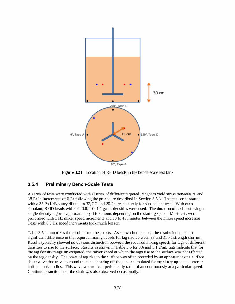
3.28
Figure 3.21. Location of RFID beads in the bench-scale test tank
3.5.4 Preliminary Bench-Scale Tests
A series of tests were conducted with slurries of different targeted Bingham yield stress between 20 and
38 Pa in increments of 6 Pa following the procedure described in Section 3.5.3. The test series started
with a 37 Pa K:B slurry diluted to 32, 27, and 20 Pa, respectively for subsequent tests. With each
simulant, RFID beads with 0.6, 0.8, 1.0, 1.1 g/mL densities were used. The duration of each test using a
single-density tag was approximately 4 to 6 hours depending on the starting speed. Most tests were
performed with 1 Hz mixer speed increments and 30 to 45 minutes between the mixer speed increases.
Tests with 0.5 Hz speed increments took much longer.
Table 3.5 summarizes the results from these tests. As shown in this table, the results indicated no
significant difference in the required mixing speeds for tag rise between 38 and 31 Pa strength slurries.
Results typically showed no obvious distinction between the required mixing speeds for tags of different
densities to rise to the surface. Results as shown in Table 3.5 for 0.6 and 1.1 g/mL tags indicate that for
the tag density range investigated, the mixer speed at which the tags rise to the surface was not affected
by the tag density. The onset of tag rise to the surface was often preceded by an appearance of a surface
shear wave that travels around the tank shearing off the top accumulated foamy slurry up to a quarter or
half the tanks radius. This wave was noticed periodically rather than continuously at a particular speed.
Continuous suction near the shaft was also observed occasionally.
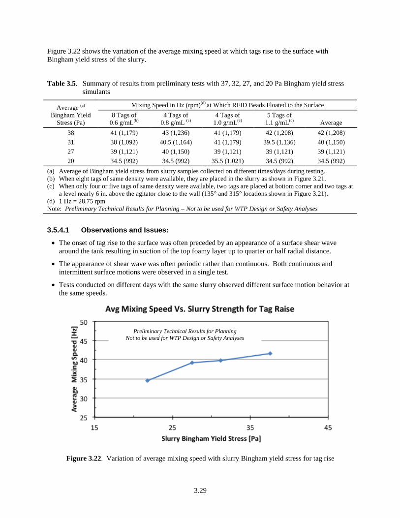
3.29
Figure 3.22 shows the variation of the average mixing speed at which tags rise to the surface with
Bingham yield stress of the slurry.
Table 3.5. Summary of results from preliminary tests with 37, 32, 27, and 20 Pa Bingham yield stress
simulants
Average (a)
Bingham Yield
Stress (Pa)
Mixing Speed in Hz (rpm)(d)
at Which RFID Beads Floated to the Surface
8 Tags of
0.6 g/mL(b)
4 Tags of
0.8 g/mL (c)
4 Tags of
1.0 g/mL(c)
5 Tags of
1.1 g/mL(c)
Average
38 41 (1,179) 43 (1,236) 41 (1,179) 42 (1,208) 42 (1,208)
31 38 (1,092) 40.5 (1,164) 41 (1,179) 39.5 (1,136) 40 (1,150)
27 39 (1,121) 40 (1,150) 39 (1,121) 39 (1,121) 39 (1,121)
20 34.5 (992) 34.5 (992) 35.5 (1,021) 34.5 (992) 34.5 (992)
(a) Average of Bingham yield stress from slurry samples collected on different times/days during testing.
(b) When eight tags of same density were available, they are placed in the slurry as shown in Figure 3.21.
(c) When only four or five tags of same density were available, two tags are placed at bottom corner and two tags at
a level nearly 6 in. above the agitator close to the wall (135° and 315° locations shown in Figure 3.21).
(d) 1 Hz = 28.75 rpm
Note: Preliminary Technical Results for Planning – Not to be used for WTP Design or Safety Analyses
3.5.4.1 Observations and Issues:
The onset of tag rise to the surface was often preceded by an appearance of a surface shear wave
around the tank resulting in suction of the top foamy layer up to quarter or half radial distance.
The appearance of shear wave was often periodic rather than continuous. Both continuous and
intermittent surface motions were observed in a single test.
Tests conducted on different days with the same slurry observed different surface motion behavior at
the same speeds.
Figure 3.22. Variation of average mixing speed with slurry Bingham yield stress for tag rise
Preliminary Technical Results for Planning
Not to be used for WTP Design or Safety Analyses
3.30
3.5.5 Summary of Key Observations and Recommendations
The following list summarizes key observations made during the tests described in this section and makes
recommendations for future testing:
The shakedown tests conducted with 20 Pa Bingham yield stress slurry and the preliminary
bench-scale tests performed with 20 to 37 Pa Bingham yield stress slurries did not show the influence
of the tags specific gravity on the required mixing speed for their rise to the surface. This result
indicates that a tag’s buoyancy is not a dominant factor for its rise to the surface, for the range of tag
density studied.
Irrespective of the specific gravity and placement location, the RFID beads often rose to the surface
whenever the mixing speed was sufficient to shear the surface layer and generate surface motion. The
mixing speed at which surface motion occurred appeared to be dependent on the Bingham yield stress
of the slurry used in the tests.
Locating tags in tests conducted with LF RFID beads and a LF reader proved to be labor intensive.
Unless the surface was continuously monitored at the right locations, there was a high probability of
missing the tags. Continuously monitoring the entire surface was not possible with the scanning
instrument setup employed in the tests.
At the end preliminary bench-scale experiments, trial tests were conducted with HF RFID beads and
an HF reader mounted on the tank at a distance 1 to 2 in. from the surface. The reader successfully
detected the tags when they reached the surface while mixing. Using HF tags and an HF reader
removes the need for manual scanning and may significantly reduce testing duration. Thus, HF tags
and an HF reader are recommending for future testing.
Bubble generation due to peroxide assisted the tags in rising to the surface during Shakedown Test 2.
To minimize the influence of sheared paths during tag insertions, tags should be inserted right after a
thorough-mixing period and with sufficient break time (about 1 hour) prior to beginning speed tests.
The number of tags inserted appeared to influence the mixing speed at which tags rose to the surface
and the slurry’s surface motion. When more tags were inserted, surface motion appeared at lower
velocities. To minimize this effect, the same number of tags should be used at the same locations in
all tests.
Significant evaporation was observed when slurry in the tank was left overnight. Thus, tags of
different densities should be tested on the same day. To avoid the effect of change in slurry
characteristics with evaporation, water should be added to make up for evaporation when tests are
carried out over several days.
Consistent wait times should be provided between the tag insertions and start of mixing.
The Valeport EM flow sensor did not record data when slurry built up on the sensor or during
non-mixing periods between the tests. However, it was not tested rigorously and all optional settings
were not explored during this work.
The fixture used for the Met-Flow UVP was not ideal and may not produce repeatable results.
Custom build fixtures at desired locations in the tank are recommended for future testing.
The Met-Flow UVP placed radially at the surface and facing the center of the vessel appeared to
provide information sensitive to the surface motion at which tags were detected.
The Met-Flow UVP placed vertically at surface (i.e., close to the wall) and facing the bottom of
vessel did not show indicate vertical flow at the mixer speed at which the tags surfaced. No
measurable net vertical movement was detected 1 in. from the wall.

3.31
The Met-Flow UVP placed vertically, midway between the wall and the mixer shaft showed net
(upward) movement as the tags were released.
Low velocities are measured near the Met-Flow UVP probe tip (about 5 mm and less), irrespective of
probe orientation or mixer speed. The extent to which these dead zones are flow dead zones (i.e., due
to the intrusiveness of the probe) or measurement dead zones (i.e., due to being in the ultrasonic near-
field) is unknown.
3.6 Conclusions
Significant progress has been made in the evaluation of RFID beads and flow sensors for the development
of the mixing metric for gas release. Shakedown tests and preliminary bench-scale tests supported the
hypothesis that surface motion typically exists at the onset of tags rise and, therefore, gas release. The
radial component of velocity at the surface appeared to be dominant in agitator mixing. The tests
attempted to find a correlation between the mixing speeds for tag rise, the specific gravity of tags, and the
Bingham yield stress of the slurry. For the range of RFID bead (representing the buoyancies of different
size bubbles) densities evaluated, the mixing speed at which the tags were released was not influenced by
the bead density. The Bingham yield stress of slurry was found to be the dominant factor for the mixing
speed at which tags rise. Results and observations presented in this section are applicable only to the
bench-scale test stands using agitator mixing employed in this effort. The applicability of these
observations to PJM mixing in actual test stands was not studied. Additional tests and engineering is
needed to apply the experimental methods and instrumentation used in this effort to PJM systems.

4.1
4.0 Evaluate Flammable Gas Consequence of Imperfect Mixing
The scope for this task was to evaluate the flammable gas consequences of imperfect mixing during
normal operations in WTP process vessels. WTP vessels are mixed to blend process fluids, suspend
solids, and release retained gases (24590-WTP-ES-ENG-09-001, Rev. 2). As required by the Basis of
Design (24590-WTP-DB-ENG-01-001, Rev. 2):
“Vessels shall provide for safe receipt, mixing, and transfer of waste as appropriate
for the particular waste properties contained in that vessel. Vessels shall be capable
of purging hydrogen in a fashion that precludes buildup of hydrogen to
concentrations above that specified in the authorization basis for the respective WTP
facility. Cooling and or heating are required based on the particular waste properties
contained in a particular vessel and to achieve required processing conditions.”
Vessel functions and mixing criteria/requirements were developed based on the functional requirements
of the vessels listed in the contract, system descriptions, operations requirements document and other
technical baseline documents. Specific to gas release, 24590-WTP-ES-ENG-09-001, Rev. 2 defines
Criteria 8:
Criteria 8 - Mix to Release Gas - (Safety related requirement)
Defines the degree of mixing (degree of solids mobilization) required to release
flammable gas that is retained in settled solids layers or non-Newtonian fluid.
This results in the functional requirement:
The PJM mixing system shall mobilize solids to release gas.
Specific to normal operations, 24590-WTP-ES-ENG-09-001, Rev. 2 states that PJM mixing is credited
for the release of hydrogen, so the frequency of operation shall be such that the quantity of hydrogen in
the waste will not exceed 1 percent in the headspace (i.e., 25 percent of the lower flammability limit
[LFL] for hydrogen) if released instantaneously.
Based on these requirements, there is a maximum allowable un-mixed region (i.e., dead zone) resulting
from imperfect mixing, such that gas release from this region will not exceed 25 percent of the LFL for
hydrogen in the vessel headspace if the retained hydrogen were released instantaneously. Therefore, this
task investigates the maximum allowable un-mixed region relative to the as-characterized physiochemical
properties of Hanford waste (i.e., as-existing and blended and treated) along with new understandings of
gas retention and release characteristics from the task described in Section 6.0.
Section 4.2 summarizes the possible spontaneous gas release mechanisms initially considered in the
evaluation. Section 4.3 presents the preliminary modeling approach, initial model evaluations, and a
comparison to preliminary test results (Section 6.3.3). The objective and success criteria that were
developed as part of the planning for this effort are given in the following section.
4.2
4.1 Objectives
TP-WTPSP-1401 identifies the following test objective for the effort on the HGR margin:
Test/Analysis Objective 9 - Evaluate Flammable Gas Consequences of Imperfect Mixing: By analysis,
evaluate the flammable gas consequences of imperfect mixing during normal operations in WTP process
vessels to provide estimates of the maximum allowable un-mixed region, which is the margin in
demonstrating 100 percent vessel motion for gas release, such that gas release from this region will not
exceed 25 percent of the LFL for hydrogen in the vessel headspace if the retained hydrogen were released
spontaneously.
The following criteria were to be used to assess the successful completion of this test/analysis objective:
calculate the maximum allowable un-mixed region (dead zone) using physicochemical properties of
Hanford waste for buoyant motion and bubble cascade (BC) releases
assess effect of PTF processing on estimates of allowed un-mixed region
include new data on BC and buoyant motion of dead zones in estimates of allowed un-mixed regions
confirm estimates of dead zone gas retention and motion by comparing with applicable experimental
results.
4.2 Spontaneous Releases from Regions of Imperfect Mixing
Hanford waste exhibits a wide range of behaviors significant to gas retention and release. Spontaneous
gas releases from dead zones in imperfectly mixed WTP process vessels are possible via the observed
significant spontaneous gas release mechanisms in Hanford waste tanks—buoyant displacement gas
release events (BDGREs). Additional postulated significant spontaneous gas release mechanisms include
BCs and the buoyant motion of dead zones in non-Newtonian yield-stress slurries.
BDGREs have been observed in six Hanford double-shell tanks (DSTs) with supernatant liquid
overlaying sediment (Hedengren et al. 2000). Some BDGREs have resulted in gas releases of sufficient
volume to exceed the LFL in the tank headspace (Meyer and Stewart 2001). Meyer and Stewart (2001)
describe BDGREs as a portion, or "gob," of the sediment layer accumulating gas until it becomes
sufficiently buoyant to overcome its weight and the yield stress of the surrounding material restraining it.
At that point it breaks away and rises through the supernatant layer. The stored gas bubbles expand as the
gob rises, failing the surrounding material, so a fraction of the gas is released from the gob into the
headspace. After releasing a portion of its gas, the remaining gob material is no longer buoyant and sinks
back to the bottom of the tank. This buoyant displacement (BD) gas release process is illustrated in
Figure 4.1. Note that the gobs depicted in the figure are staggered for clarity only; based on temperature
profiles, the actual process is believed to occur more or less vertically.
The Hanford waste tanks with observed BDGREs have sediments with yield stress in shear on the order
of 100 to a few hundred pascals, and small-scale experiments have shown BDGREs in sediments on the
order of 10 Pa (Meyer et al. 1997). Based on more than 60 years of process data, Meacham et al. (2014)
argue that the BDGRE phenomena does not occur for wastes with sufficiently high shear strength. For
weaker materials, including the sediments in BDGRE tanks, the phenomena of BC gas release has also
been observed experimentally as described in detail in Section 6.1. Figure 6.1 in that section depicts a BC
event.
1 Gauglitz PA. 2015. Test Plan for Hydrogen Gas Release from Vessels Technical Issue Support.
TP-WTPSP-140, Rev. 0. Pacific Northwest National Laboratory.
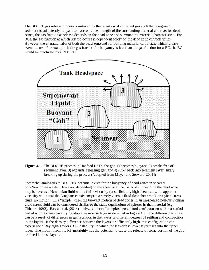
4.3
The BDGRE gas release process is initiated by the retention of sufficient gas such that a region of
sediment is sufficiently buoyant to overcome the strength of the surrounding material and rise; for dead
zones, the gas fraction at release depends on the dead zone and surrounding material characteristics. For
BCs, the gas fraction at which release occurs is dependent solely on the dead zone characteristics.
However, the characteristics of both the dead zone and surrounding material can dictate which release
event occurs. For example, if the gas fraction for buoyancy is less than the gas fraction for a BC, the BC
would be precluded by a BDGRE.
Figure 4.1. The BDGRE process in Hanford DSTs: the gob 1) becomes buoyant, 2) breaks free of
sediment layer, 3) expands, releasing gas, and 4) sinks back into sediment layer (likely
breaking up during the process) (adopted from Meyer and Stewart [2001])
Somewhat analogous to BDGREs, potential exists for the buoyancy of dead zones in sheared
non-Newtonian waste. However, depending on the shear rate, the material surrounding the dead zone
may behave as a Newtonian fluid with a finite viscosity (at sufficiently high shear rates, the apparent
viscosity will equal the Bingham consistency), extremely viscous fluid (low shear rate), or a yield stress
fluid (no motion). In a “simple” case, the buoyant motion of dead zones in an un-sheared non-Newtonian
yield-stress fluid can be considered similar to the static equilibrium of spheres in that material (e.g.,
Chhabra 1992). Rassat et al. (2014) analyzes a more “complex” postulated configuration within a settled
bed of a more-dense layer lying atop a less-dense layer as depicted in Figure 4.2. The different densities
can be a result of differences in gas retention in the layers or different degrees of settling and compaction
in the layers. If the density difference between the layers is sufficiently high, this configuration can
experience a Rayleigh-Taylor (RT) instability, in which the less-dense lower layer rises into the upper
layer. The motion from the RT instability has the potential to cause the release of some portion of the gas
retained in these layers.

4.4
The liquid layers shown in Figure 4.2 make this example representative of the off-normal cases (i.e.,
Cases 2, 3, and 4) shown in Figure 1.1. A scenario could also be postulated for the normal Newtonian
condition of Figure 1.1 wherein imperfect mixing of subsequent batches could potentially result in a
more-dense layer lying atop a less-dense layer. If no supernatant liquid layer were present in the
examples shown in Figure 4.2, those examples would be representative of imperfect mixing in normal
non-Newtonian or the off-normal scenario (i.e., Case 1 in Figure 1.1). Without buoyancy in the
supernatant liquid layer (or with no supernatant layer), Rassat et al. (2014) shows “negligible gas release
events” and “small gas release events” as the result of in-sediment buoyant motion. A “potentially large
gas release events” results from buoyant motion in the supernatant liquid (i.e., a BDGRE).
Figure 4.2. Evolution of an RT instability of a less-dense waste layer, due to retained gas bubbles
(depicted as blue spheres), rising in a more-dense layer, and subsequent gas release event
(GRE) scenarios (adopted from Rassat et al. 2014)
The described spontaneous gas release mechanisms are referenced to the conditions depicted in
Figure 1.1. With imperfect mixing during normal operations, BDGREs are most probable for the
Newtonian conditions, and BCs can occur in both the non-Newtonian and Newtonian conditions
depending on the yield stress of the undisturbed region. The buoyant motion of dead zones can occur in
both conditions as described above. For the off-normal scenario cases shown in Figure 1.1, BDGREs can
occur for Cases 2 through 4. BCs can occur in Cases 1, 2, and 3, but may be precluded by the waste yield
stress for Case 4. The buoyant motion of a dead zone can occur in any case.
The scope of this task was to evaluate the flammable gas consequences of imperfect mixing during
normal operations in WTP process vessels. As described, the spontaneous gas release mechanisms
depend on waste configuration. Various dead zone scenarios possible during normal operation were
identified at a June 27, 2014 meeting as documented in Appendix B. The preliminary identified scenarios
are listed in Table 4.1 together with the potential spontaneous gas release mechanism(s). BCs are
indicated as the most common possible spontaneous release mechanism. As described in Section 6.1,
limited data are available for understanding this mechanism. Likewise, data addressing the phenomena of
4.5
buoyant dead zone motion specific to the described scenarios is limited and an approach for developing
experimental data and a better understanding of dead zone motion is described in Section 6.3.
Table 4.1. Dead zone scenarios resulting from imperfect mixing during normal operations
Dead Zone Scenario
Possible Spontaneous Gas
Release Mechanism
Buoyant motion of lower dead zone BDGRE, BC
Dead zone above PJMs BC
Thin zone on vessel walls (and other structure surfaces) BDGRE, BC
Upper dead zone in non-Newtonian vessel (e.g., more peripheral of PJMs) BC
Floating crusts in PJM vessels BC
4.3 Preliminary Modeling Approach, Results, and Comparison to Test Data
The initial bounding calculation for the flammable gas consequences of imperfect mixing during normal
operations in WTP process vessels to determine the maximum allowable un-mixed region was a simple
volume comparison. Specifically, if the maximum measured Hanford waste retained gas fraction
contained the maximum measured Hanford fraction of hydrogen in the retained gas, what is the maximum
allowable un-mixed region such that the instantaneous release of 100 percent of this gas would not exceed
25 percent of the LFL of hydrogen in the tank headspace? This maximum allowable un-mixed region
relative to the waste volume can be expressed, in percent, as
100
P
P
VH
V005.0
V
V
HS
DZ
W2
HS
W
DZ
4.1
where V = volume
P = pressure
DZ = dead zone
W = waste
HS = headspace
α = retained gas volume fraction
[H2] = hydrogen volume fraction in retained gas.
Mahoney and Stewart (2002) specify that pure hydrogen in air has an LFL of 4 volume percent (vol%).
The 0.005 VHS term represents 50 percent of 25 percent of the LFL of hydrogen (i.e., 12.5 percent of the
LFL of hydrogen) as 24590-WTP-M4C-V11T-00011 assumes that sufficient headspace purge is operated
to maintain the vessel headspace at or below 12.5 percent of the LFL of hydrogen. Therefore, the
maximum allowable hydrogen volume in the waste is the same, 12.5 percent, to remain below 25 percent
LFL in the headspace.
The maximum measured Hanford waste retained gas volume fraction, taken from Gauglitz et al. (1996), is
0.54. Retained gas composition measurements are available for only a limited set of the Hanford salt
slurry waste tanks (Mahoney et al. 2000). Wells et al. (2013) combined these data with uncertainties to
define a distribution. The data range from 0.03 to 1 hydrogen volume fraction and a roughly bimodal
distribution is indicated with generalized modes at approximately 0.30 and 0.65. The maximum fraction
of 1 is used here. With a negligible pressure ratio and equal headspace and waste volumes, the maximum

4.6
allowable un-mixed region relative to the waste volume is approximately 1 percent. Reduction of the
headspace volume to a representative WTP process vessel minimum of VHS/VW of 0.15 (e.g.,
24590-WTP-M4C-V11T-00011) reduces the ratio to approximately 0.1 percent.
Besides the remarkably small allowable dead zone volume, a fundamental issue with this simple
bounding approach is the physical plausibility of retaining 50 percent gas in a dead zone of the WTP
process vessel waste conditions during normal operations. Therefore, preliminary modeling focused on
the buoyant motion of dead zones in an un-sheared, non-Newtonian yield-stress fluid, specifically relative
to the static equilibrium of spheres in that material.
Appendix B of Gauglitz et al. (2009) compares the literature basis of the static equilibrium and motion of
spheres in non-Newtonian fluids to available data from Hanford tank waste. A dimensionless parameter
YG, the critical gravity yield number (Attapatu et al. 1995; Chhabra 1992), is defined by equating the
buoyant weight of a sphere to the vertical component of the yield stress (in shear) acting over the surface
of the sphere, or
gdYG
4.2
where
= yield stress in shear
g = gravitational acceleration
d = sphere diameter
= difference in the sphere and bulk fluid densities.
The most probable value for YG may be given by Attapatu et al. (1995), which reports that the available
experimental data indicate YG is approximately 0.061. Gauglitz et al. (2009) concluded that this value is
plausible in comparison to actual waste data. Note that Rassat et al. (2014) uses a similar
non-dimensional group to define the onset of an RT instability for the waste configuration with a more-
dense settled bed layer lying atop a less-dense layer.
With Eq. 4.2, the physical plausibility of having a dead zone with a gas fraction of 0.54 for the bounding
calculation can be evaluated for the specific condition represented and a more representative maximum
allowable un-mixed region (dead zone) relative to the waste volume can be defined. The dead zone
scenario most applicable to this condition is the buoyant motion of the lower dead zone (see Table 4.1).
For this analysis, the density of the gas-free dead zone and the surrounding material are assumed to be
equal at s, so of Eq. 4.2 can be rewritten as s. Therefore, from Eq. 4.2, the retained gas fraction
at which the dead zone will move and as a result potentially release its gas is decreased for
larger-diameter dead zones. In the buoyant motion of lower dead zone scenario, the most probable
location of the dead zones on the tank bottom is along the vessel wall between the PJMs as depicted in
Figure 4.3. For the example six PJM system, there are therefore six potential dead zones as shown by the
white regions in Figure 4.3 corresponding to locations of the lowest applied wall stress. This dispersion
of the dead zone volume into separate regions is conservative as described; smaller diameter dead zones
will have larger retained gas fractions at the onset of motion.
An example of experimental evidence of potential bottom dead zone shape is provided in Figure 4.4. The
image in Figure 4.4 was taken during simulant removal at the completion of gas release testing with a
non-Newtonian (3 to 30 Pa Bingham yield stress) chemical waste simulant (Stewart et al. 2007).
Although the PJM array and nozzle orientation are different than the computational fluid dynamic (CFD)
example of Figure 4.3, the implication of “bat wing” shapes between the PJMs along the vessel wall is
evident. The vertical white tubes are air spargers.

4.7
Figure 4.3. Depiction of dead zones, shown as white regions, between PJMs on the vessel bottom for the
scenario of buoyant motion of lower dead zones. Calculations of the wall shear stress in a
16 ft diameter, six PJM vessel were performed using a commercial CFD code (Star-CCM+
Version 8.06.007, CD-Adapco).1
The Basis of Design (24590-WTP-DB-ENG-01-001), which defines the design requirements and design
codes and standards that will serve as the basis for the continued design of the WTP, specifies that
the WTP will use process controls to condition the slurry viscosity and shear strength for leached,
washed, and concentrated waste to be within the range of 6 cP and 6 Pa to 30 cP and 30 Pa as the
lower and upper bounds, respectively.
1 Recknagle KP and MJ Minette. January 28, 2015. Flow Field Comparison of PJM-Mixed Vessels Relative to Gas
Release. PNNL-SA-107799.

4.8
Figure 4.4. Dead zones on vessel bottom post-experiment during simulant removal (Stewart et al. 2007)
The preliminary analysis used the conservative limit of 30 Pa for the yield stress in shear (maximum
retained gas fraction, Eq. 4.2; thus, minimum dead zone volume), 6 spherical dead zones, and a
representative material density of 1.4 g/mL. A 16 ft diameter (D) vessel was evaluated with a waste
volume equal to 3D
4
. The resultant gas fraction in a dead zone for motion, together with the total dead
zone fraction of waste volume, is shown in Figure 4.5. Clearly, the bounding calculation using a gas
volume fraction of 0.54 resulting in a 1 percent waste-volume dead zone limit (see earlier discussion in
this section for the basis of this bounding estimate) at equal headspace and waste volumes (denoted by the
vertical orange dashed line in the figure), over-represents the gas fraction at which the dead zone would
have buoyant motion. Specifically, Figure 4.5 shows the calculated void fraction for the onset of motion
of approximately 0.05 gas volume fraction at the conditions of 1 percent dead zone volume fraction (at a
dead zone diameter of about 0.7 m).
The bulk gas volume fraction, the dead zone gas volume fraction relative to the total waste volume, is
shown in Figure 4.6. This gas volume fraction can be directly related to the minimum allowable head
space volume, shown in Figure 4.6 as the fraction VHS/VW, at the conditions when 100 percent
simultaneous release from all six dead zones gives 12.5 percent of the LFL. The approximate 0.05 gas
volume fraction example given previously (dead zone diameter of about 0.7 m) has a minimum allowable
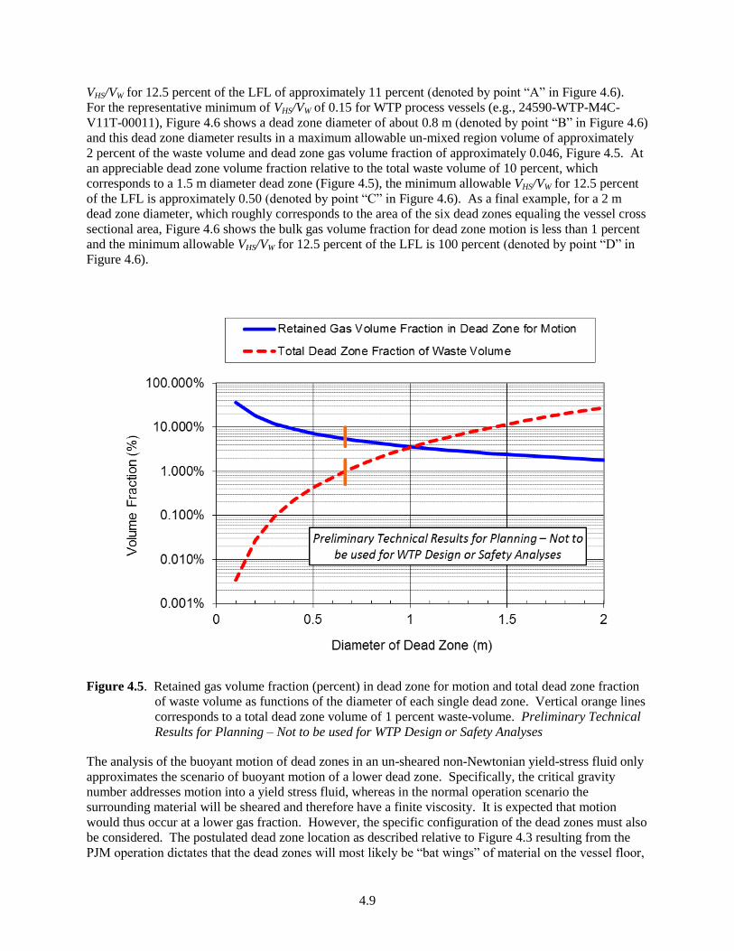
4.9
VHS/VW for 12.5 percent of the LFL of approximately 11 percent (denoted by point “A” in Figure 4.6).
For the representative minimum of VHS/VW of 0.15 for WTP process vessels (e.g., 24590-WTP-M4C-
V11T-00011), Figure 4.6 shows a dead zone diameter of about 0.8 m (denoted by point “B” in Figure 4.6)
and this dead zone diameter results in a maximum allowable un-mixed region volume of approximately
2 percent of the waste volume and dead zone gas volume fraction of approximately 0.046, Figure 4.5. At
an appreciable dead zone volume fraction relative to the total waste volume of 10 percent, which
corresponds to a 1.5 m diameter dead zone (Figure 4.5), the minimum allowable VHS/VW for 12.5 percent
of the LFL is approximately 0.50 (denoted by point “C” in Figure 4.6). As a final example, for a 2 m
dead zone diameter, which roughly corresponds to the area of the six dead zones equaling the vessel cross
sectional area, Figure 4.6 shows the bulk gas volume fraction for dead zone motion is less than 1 percent
and the minimum allowable VHS/VW for 12.5 percent of the LFL is 100 percent (denoted by point “D” in
Figure 4.6).
Figure 4.5. Retained gas volume fraction (percent) in dead zone for motion and total dead zone fraction
of waste volume as functions of the diameter of each single dead zone. Vertical orange lines
corresponds to a total dead zone volume of 1 percent waste-volume. Preliminary Technical
Results for Planning – Not to be used for WTP Design or Safety Analyses
The analysis of the buoyant motion of dead zones in an un-sheared non-Newtonian yield-stress fluid only
approximates the scenario of buoyant motion of a lower dead zone. Specifically, the critical gravity
number addresses motion into a yield stress fluid, whereas in the normal operation scenario the
surrounding material will be sheared and therefore have a finite viscosity. It is expected that motion
would thus occur at a lower gas fraction. However, the specific configuration of the dead zones must also
be considered. The postulated dead zone location as described relative to Figure 4.3 resulting from the
PJM operation dictates that the dead zones will most likely be “bat wings” of material on the vessel floor,
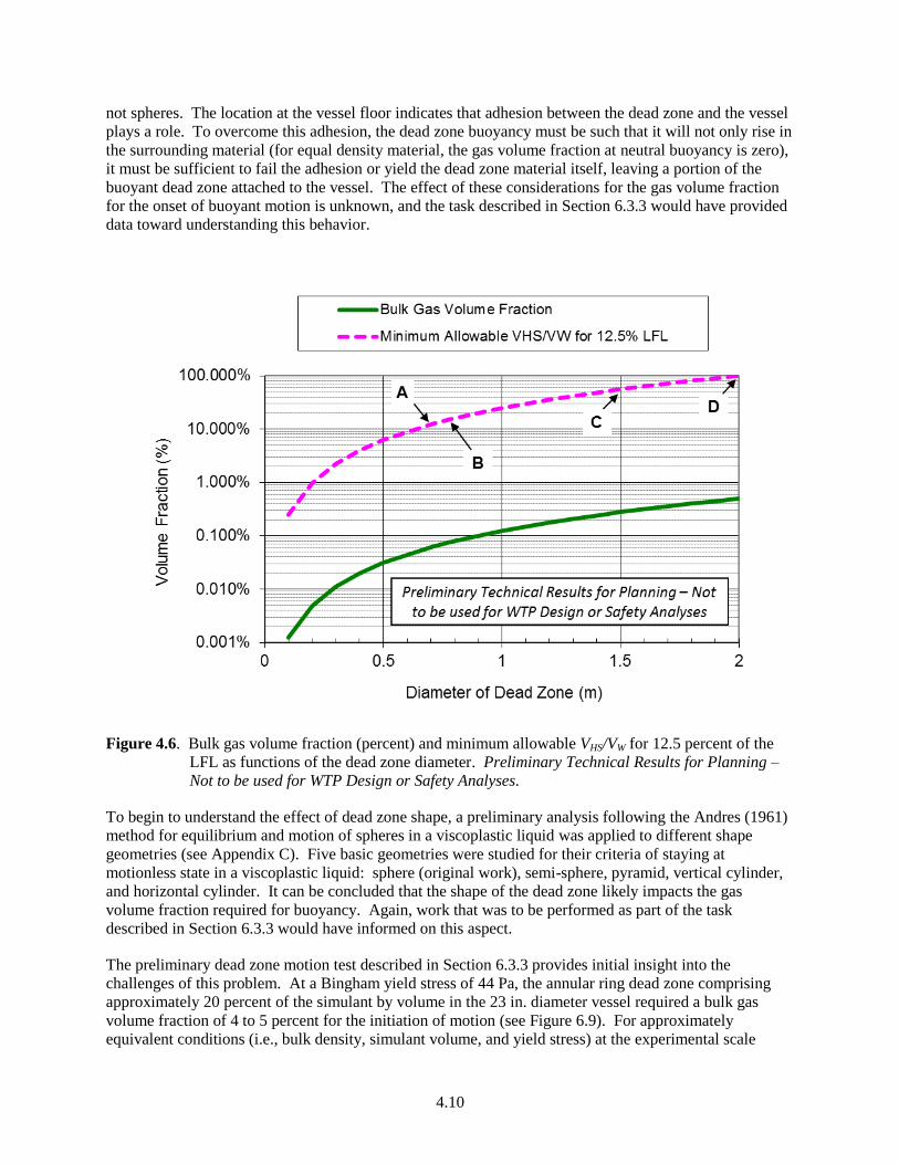
4.10
not spheres. The location at the vessel floor indicates that adhesion between the dead zone and the vessel
plays a role. To overcome this adhesion, the dead zone buoyancy must be such that it will not only rise in
the surrounding material (for equal density material, the gas volume fraction at neutral buoyancy is zero),
it must be sufficient to fail the adhesion or yield the dead zone material itself, leaving a portion of the
buoyant dead zone attached to the vessel. The effect of these considerations for the gas volume fraction
for the onset of buoyant motion is unknown, and the task described in Section 6.3.3 would have provided
data toward understanding this behavior.
Figure 4.6. Bulk gas volume fraction (percent) and minimum allowable VHS/VW for 12.5 percent of the
LFL as functions of the dead zone diameter. Preliminary Technical Results for Planning –
Not to be used for WTP Design or Safety Analyses.
To begin to understand the effect of dead zone shape, a preliminary analysis following the Andres (1961)
method for equilibrium and motion of spheres in a viscoplastic liquid was applied to different shape
geometries (see Appendix C). Five basic geometries were studied for their criteria of staying at
motionless state in a viscoplastic liquid: sphere (original work), semi-sphere, pyramid, vertical cylinder,
and horizontal cylinder. It can be concluded that the shape of the dead zone likely impacts the gas
volume fraction required for buoyancy. Again, work that was to be performed as part of the task
described in Section 6.3.3 would have informed on this aspect.
The preliminary dead zone motion test described in Section 6.3.3 provides initial insight into the
challenges of this problem. At a Bingham yield stress of 44 Pa, the annular ring dead zone comprising
approximately 20 percent of the simulant by volume in the 23 in. diameter vessel required a bulk gas
volume fraction of 4 to 5 percent for the initiation of motion (see Figure 6.9). For approximately
equivalent conditions (i.e., bulk density, simulant volume, and yield stress) at the experimental scale
4.11
where the annular dead zone volume with the gas volume at the time of the GRE (19 percent) is equated
to a sphere diameter, the required gas volume fraction calculated via Eq. 4.2 is approximately 0.14, which
corresponds to a bulk gas volume fraction of approximately 3 percent. These calculated results for a
different geometry are comparable with the experimental result. At the 16 ft tank diameter example
however, the required gas volume fraction is calculated to be approximately 0.02 (bulk gas volume
fraction of approximately 0.4 percent). The disparity in the calculations for the different scales (with both
the 23 in. and 16 ft diameter vessels having 20 percent of their volume as a sphere) results directly from
the functionality of the critical gravity yield number. From Eq. 4.2, the retained gas fraction at which
the dead zone will move is decreased for larger-diameter dead zones.
These preliminary calculations, both the bounding calculation and analysis of the buoyant motion of dead
zones in an un-sheared non-Newtonian yield-stress fluid, provide approximate effects of potential
behaviors. As demonstrated by comparison to the preliminary test data, significant uncertainties exist in
the approaches—which were to be addressed via testing. Accurate, non-bounding estimates of the
maximum allowable un-mixed or dead zone region such that gas release from this region will not exceed
25 percent of the LFL for hydrogen in the vessel headspace if the retained hydrogen were released
spontaneously requires specific test data for the scenarios at conditions representing the Hanford waste.
The Hanford waste exhibits a wide range of behaviors significant to gas retention and release, and the
effect of treatment processes on these behaviors is not well understood. A robust mixing system is thus
likely required to maintain the specified gas inventory during normal operations.

5.1
5.0 Simulant Selection for Quantifying Gas Release in Testing and Comparison to Actual Waste Behavior
Tank waste simulants, typically physical simulants that replicate target physical properties have been used
as non-radiological stand-in materials to enable evaluation of gas retention and release mechanics at
engineering scales. However, little is known about the gas retention and release in actual sludge material,
especially for events either initiated by or occurring under shear. The issue of non-radiological simulant
relevance (with respect to gas release studies) was recently raised as part of plans to resolve T1 (Allen
2014). In particular, the T1 resolution plan poses the following two questions:
Do the simulants used in previous gas release testing adequately represent actual waste at plant
conditions?
What is the most suitable simulant for any planned gas release testing?
Simulant selection activities were intended to address the representativeness of simulants for gas release
testing and to recommend a simulant for experimental testing supporting T1 resolution (as well as
resolution of other technical issues). This section summarizes simulant selection efforts to date and
provides a description of the program approach for evaluating simulants, preliminary findings, and the
results of scoping tests performed in support of simulant recommendation development. The objectives
and success criteria developed as part of the planning for this effort are given in the following section.
5.1 Test Objectives and Success Criteria
TP-WTPSP-1401 identifies the following test objective for the effort on resolving T1 simulant needs:
Test Objective 6 – Gas Release Simulant Recommendation: Recommend components and one or
more recipes for a physical simulant for gas release testing being conducted to resolve Technical
Issue T4 – PJM Vessel Mixing and Control (T4) and related T1 studies.
Test Objective 7 – Technical Basis for Selected Simulant: Provide a basis for why each physical
simulant recommended is suitable for gas release testing, the basis for why it can be considered
representative of actual waste, where it can be applied, and any potential limitations.
Test Objective 8 – Comparison to Actual Waste Behavior: If sufficient data exist to compare
simulant gas retention and release behavior to that of actual waste, provide a basis for why the
recommended physical simulant is representative of or provides a conservative analogue of actual
waste gas retention and release behavior.
Achievement of these test objectives were to be gaged by satisfaction of the success criteria. These
criteria are as follows:
Success Criterion for Objective 6:
One or more simulant recipes have been recommended for large-scale gas release testing to resolve
T4 and T1.
1 Gauglitz PA. 2015. Test Plan for Hydrogen Gas Release from Vessels Technical Issue Support. TP-WTPSP-
140, Rev. 0, Pacific Northwest National Laboratory.

5.2
Success Criteria for Objective 7:
A literature review of gas retention and release behavior in mixed systems has been conducted and
provides sufficient observational evidence or experimental metrics on which to develop physical
simulants that are “suitable” for scaled gas retention and release testing.
The gas retention and release behavior of physical simulant recipes (primarily non-Newtonian
clay-in-water slurries and select chemical simulants) considered has been evaluated and quantified.
Simulant recipes showing suitable gas retention and release have been down-selected for additional
testing.
For the set of down-selected simulant recipes, the gas release behavior has been evaluated at different
scales for suitability.
For the set of down-selected simulant recipes, key physical properties (e.g., density, rheology, and gas
release proclivity) have been measured and their stability (e.g., with respect to shear, exposure to air,
and drying) has been established.
Success Criterion for Objective 8:
Actual waste gas retention and release data have been evaluated and, if suitable data exist, compared
to that of the recommended simulant recipe(s).
5.2 Technical Approach
The overall focus of simulant selection testing is to recommend one or more simulant recipes for
large-scale gas release tests addressing T1 and T4 resolution. The proposed approach is to review the
literature and build a database of historical GREs observed in the tanks and previous flammable gas
release studies involving physical simulants and actual waste samples. This database was to be
accompanied by available waste physical properties data. The gas release and physical property database
will form the basis for developing physical simulants using non-hazardous materials including, but not
necessarily limited to, mixtures of kaolin and bentonite clay powders in water. Physical simulant recipes
were planned to be selected such that the final simulant targets physical properties (e.g., bulk density,
yield stress, and consistency) suitable for gas release testing and appropriately representative of actual
waste feeds and processed slurries. To achieve physical property targets, soluble salts may be added to
the liquid phase. However, use of salts for the baseline simulant recipe will be avoided if possible as salts
can interfere with some of the instruments (i.e., conductivity probes and level sensors) used in PJM
testing.
While simulant selection efforts will evaluate and document the physical properties of waste simulants,
the ultimate goal of testing is to provide a simulant with gas release behavior conservatively
representative of actual waste. To this end, simulant selection efforts will evaluate the rate and magnitude
of gas generation, retention, and release resulting from mixing down-selected simulant recipes with H2O2
solution. Although H2O2 decomposition is the primary candidate for gas generation methods, other
methods (e.g., air entrainment and reactive powder addition) may be considered.
Figure 5.1 shows the conceptual test apparatus for gas generation and release testing. The apparatus
consists of two vessels: 1) a sealed slurry reservoir and 2) a gas capture vessel. The slurry reservoir
allows for an overhead mixer and impeller, which can be used to mix the slurry or effect shear-induced
release of gas from the slurry. H2O2 is pumped into the test slurry at a location near the mixing impeller
to maximize dispersion of the H2O2, using a syringe pump. Two modes of operation are proposed to
assess gas release of down-selected simulants:
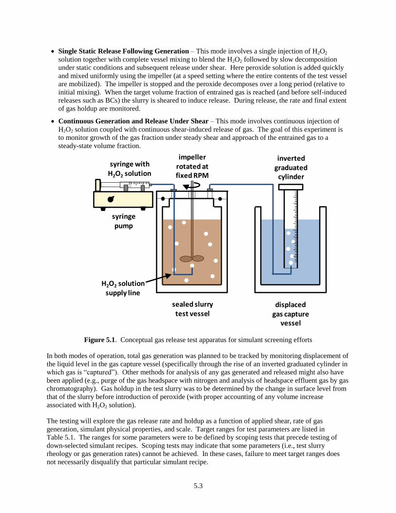
5.3
Single Static Release Following Generation – This mode involves a single injection of H2O2
solution together with complete vessel mixing to blend the H2O2 followed by slow decomposition
under static conditions and subsequent release under shear. Here peroxide solution is added quickly
and mixed uniformly using the impeller (at a speed setting where the entire contents of the test vessel
are mobilized). The impeller is stopped and the peroxide decomposes over a long period (relative to
initial mixing). When the target volume fraction of entrained gas is reached (and before self-induced
releases such as BCs) the slurry is sheared to induce release. During release, the rate and final extent
of gas holdup are monitored.
Continuous Generation and Release Under Shear – This mode involves continuous injection of
H2O2 solution coupled with continuous shear-induced release of gas. The goal of this experiment is
to monitor growth of the gas fraction under steady shear and approach of the entrained gas to a
steady-state volume fraction.
Figure 5.1. Conceptual gas release test apparatus for simulant screening efforts
In both modes of operation, total gas generation was planned to be tracked by monitoring displacement of
the liquid level in the gas capture vessel (specifically through the rise of an inverted graduated cylinder in
which gas is “captured”). Other methods for analysis of any gas generated and released might also have
been applied (e.g., purge of the gas headspace with nitrogen and analysis of headspace effluent gas by gas
chromatography). Gas holdup in the test slurry was to be determined by the change in surface level from
that of the slurry before introduction of peroxide (with proper accounting of any volume increase
associated with H2O2 solution).
The testing will explore the gas release rate and holdup as a function of applied shear, rate of gas
generation, simulant physical properties, and scale. Target ranges for test parameters are listed in
Table 5.1. The ranges for some parameters were to be defined by scoping tests that precede testing of
down-selected simulant recipes. Scoping tests may indicate that some parameters (i.e., test slurry
rheology or gas generation rates) cannot be achieved. In these cases, failure to meet target ranges does
not necessarily disqualify that particular simulant recipe.
sealed slurry test vessel
displaced gas capture
vessel
inverted graduated
cylinder
impeller rotated at fixed RPM
syringe pump
syringe with H2O2 solution
H2O2 solution supply line
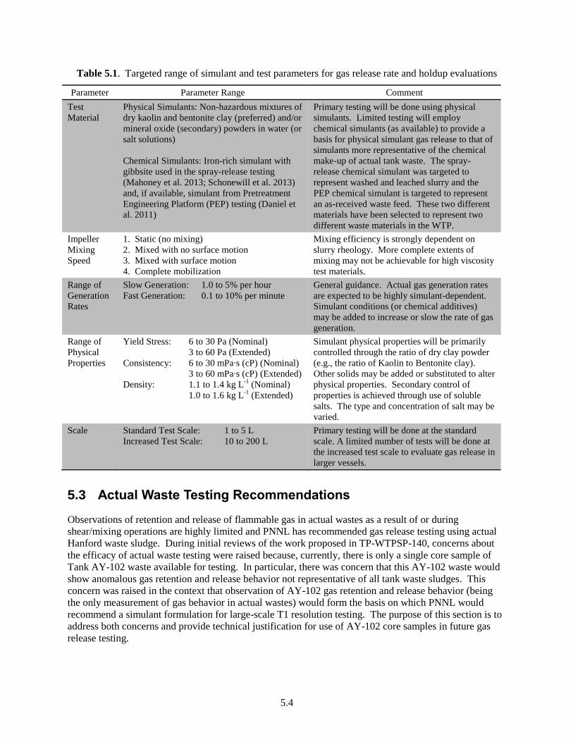
5.4
Table 5.1. Targeted range of simulant and test parameters for gas release rate and holdup evaluations
Parameter Parameter Range Comment
Test
Material
Physical Simulants: Non-hazardous mixtures of
dry kaolin and bentonite clay (preferred) and/or
mineral oxide (secondary) powders in water (or
salt solutions)
Chemical Simulants: Iron-rich simulant with
gibbsite used in the spray-release testing
(Mahoney et al. 2013; Schonewill et al. 2013)
and, if available, simulant from Pretreatment
Engineering Platform (PEP) testing (Daniel et
al. 2011)
Primary testing will be done using physical
simulants. Limited testing will employ
chemical simulants (as available) to provide a
basis for physical simulant gas release to that of
simulants more representative of the chemical
make-up of actual tank waste. The spray-
release chemical simulant was targeted to
represent washed and leached slurry and the
PEP chemical simulant is targeted to represent
an as-received waste feed. These two different
materials have been selected to represent two
different waste materials in the WTP.
Impeller
Mixing
Speed
1. Static (no mixing)
2. Mixed with no surface motion
3. Mixed with surface motion
4. Complete mobilization
Mixing efficiency is strongly dependent on
slurry rheology. More complete extents of
mixing may not be achievable for high viscosity
test materials.
Range of
Generation
Rates
Slow Generation: 1.0 to 5% per hour
Fast Generation: 0.1 to 10% per minute
General guidance. Actual gas generation rates
are expected to be highly simulant-dependent.
Simulant conditions (or chemical additives)
may be added to increase or slow the rate of gas
generation.
Range of
Physical
Properties
Yield Stress: 6 to 30 Pa (Nominal)
3 to 60 Pa (Extended)
Consistency: 6 to 30 mPa∙s (cP) (Nominal)
3 to 60 mPa∙s (cP) (Extended)
Density: 1.1 to 1.4 kg L-1
(Nominal)
1.0 to 1.6 kg L-1
(Extended)
Simulant physical properties will be primarily
controlled through the ratio of dry clay powder
(e.g., the ratio of Kaolin to Bentonite clay).
Other solids may be added or substituted to alter
physical properties. Secondary control of
properties is achieved through use of soluble
salts. The type and concentration of salt may be
varied.
Scale Standard Test Scale: 1 to 5 L
Increased Test Scale: 10 to 200 L
Primary testing will be done at the standard
scale. A limited number of tests will be done at
the increased test scale to evaluate gas release in
larger vessels.
5.3 Actual Waste Testing Recommendations
Observations of retention and release of flammable gas in actual wastes as a result of or during
shear/mixing operations are highly limited and PNNL has recommended gas release testing using actual
Hanford waste sludge. During initial reviews of the work proposed in TP-WTPSP-140, concerns about
the efficacy of actual waste testing were raised because, currently, there is only a single core sample of
Tank AY-102 waste available for testing. In particular, there was concern that this AY-102 waste would
show anomalous gas retention and release behavior not representative of all tank waste sludges. This
concern was raised in the context that observation of AY-102 gas retention and release behavior (being
the only measurement of gas behavior in actual wastes) would form the basis on which PNNL would
recommend a simulant formulation for large-scale T1 resolution testing. The purpose of this section is to
address both concerns and provide technical justification for use of AY-102 core samples in future gas
release testing.
5.5
Waste in Tank AY-102 is composed of a small amount of original sludge waste (types BL and PL2) and a
significant fraction of waste transferred from Tank C-106 (types AR, CWP1, BL, TBP, and unidentified)
(Reynolds 1997; Carothers 1998; WRPS 2009).1 The blend of materials in AY-102 does not match that
of any other sludge in the tank farms and is not representative of any waste grouping. Despite the atypical
make-up of Tank AY-102 contents, PNNL has proposed bench-scale gas retention and release testing of
core sludge retrieved from Tank AY-102. The core material is of interest for testing for several reasons:
Waste in Tank AY-102 is sludge and is therefore relevant because tank waste sludge is the target of
study for T1 simulant development and testing (as opposed to saltcake wastes where WTP-relevant
hydrogen flammability issues can be resolved through dilution prior to transfer).
No direct laboratory experiments using Hanford actual waste evaluate the ability of mixing (i.e.,
shearing) to release gas; therefore, testing AY-102 waste would provide new and valuable
information useful for simulant development and evaluation.
AY-102 waste was originally scheduled for waste feed delivery with no further blending. WTP
would have directly processed this waste without modification. Its gas retention and release behavior
could therefore be directly applicable to WTP processing operations handling this waste stream.
Study of AY-102 waste could provide useful and directly applicable information.
Washington River Protection Solutions (WRPS) has used AY-102 gas retention and release behavior
as part of the basis for gaging gas release from Hanford waste sludge waste. AY-102 behavior
formed part of the technical basis for the recent modification to the flammable-gas portion of the
Documented Safety Analysis (DSA) for Hanford tank farm operations (see Meacham et al. 2014).
The DSA modification is limited to sludge waste that exhibits the following specific process data:
– has no evidence of large spontaneous GREs
– has reached a balance between gas retention and release at a retained gas content of about 8 vol%
or less
– has rapid gas transport
– exhibits rapid settling to a configuration similar to that of the source tank.
AY-102 is the only Hanford waste tank with process data demonstrating all four of these characteristics.
To restate, AY-102 waste is the only Hanford waste tank with process data that demonstrates all four of
the requirements for sludge waste gas retention and release behavior in the DSA for Hanford tank farm
operations.
In stating these reasons, it is understood that AY-102 gas retention and release behavior may not be
representative of other Hanford wastes. Indeed, no single gas retention and release behavior is expected
to fully describe the potential range of behaviors possible in Hanford waste sludges. WRPS has evaluated
gas retention in tank waste sludges and saltcakes for management and mitigation of hydrogen issues when
storing the wastes in the tank farms (Meacham et al. 2014). WRPS has identified a broad range of
behaviors, including distinct gas retention behaviors for sludge and saltcake slurries, variation in the
maximum fraction of gas retained (for both sludge and saltcake slurry waste classes), and differences in
the ease in which gas can be released upon mixing and transfer of the waste material. It is therefore
unlikely that that all Hanford wastes will show a single gas retention and release behavior under mixing
conditions and that any tank will be representative of the spectrum of release behaviors.
The approach for addressing the T1 issue, at the time that work was suspended, was to focus on
identifying a single simulant for scaled gas release and retention testing (although the potential for
1 Definitions for waste types BL, PL2, AR, CWP1, and TBP may be found in Appendix B of Wells et al. (2007).

5.6
multiple simulant recommendations has not been ruled out). The basis for simulant selection would be
developed under simulant selection testing activities, which were expected to rely, in part, on information
gained from testing of actual waste as to the reasonableness of the simulant(s) selected for scaled testing.
The selected simulant should capture the mechanics of gas retention and release in actual wastes. As
stated above, no well-defined or controlled experiments are documented in which actual wastes were
allowed to grow bubbles and then be sheared to effect release of those bubbles. Thus, any simulants
developed will have no experimental basis on which to compare the range of release behaviors shown by
those simulant systems to actual waste.
Recent gas release studies, undertaken jointly by WRPS and PNNL to support DSA modifications to
address the deep sludge gas release event (DSGRE) release scenario, used process knowledge of waste
behavior in the Hanford tank farms to underpin expectations of gas retention and release under static
conditions. Thus, the DSGRE issue could be resolved simply by evaluating whether gas retention
mechanisms change when storing quantities of sludge at depths that exceeded the historical operating
ranges. In contrast, the WTP does not have any operating history to use as a technical basis for
quantifying gas retention and release in actual wastes during PJM mixing operations and upset conditions.
PNNL continues to recommend AY-102 waste testing, but not to defensibly establish gas retention and
release behavior in actual wastes in WTP vessels. Instead, AY-102 waste testing will provide
observational evidence to establish the reasonableness of the simulant selected relative to other simulants
and the AY-102 sample. For example, testing may find that AY-102 falls within the gas release
behaviors (quantified by both the rate and extent of release of entrained bubbles) of both existing and
newly developed gas release simulants. This would provide a basis on which simulant selection could be
gaged, as researchers could quantify the deviation of the simulant from the single observation of actual
waste release behavior relative to the full spectrum of release behaviors observed in testing. On the other
hand, if gas release in actual waste showed an extent and rate of release that fell outside of the ranges
shown by existing simulants, then it demonstrates weakness in the current simulant recommendations
(including alternate recommendations that could be made).
Overall, the purpose of testing actual waste was not to validate the use of AY-102 waste such that test
results can be extended to other wastes. The purpose is to show that the current range of simulant
considered for scaled gas release testing represents any waste behavior and to provide a metric (albeit a
single metric) against which the selected simulant can be considered and the need for simulant
refinement.
5.4 Models for Interpreting Gas Release Rates and Steady-State Holdup
Basic expressions for interpreting steady-state holdup were developed as part of scoping efforts
evaluating experimental means of interpreting simulant selection experimental gas release data that would
be generated using the test apparatus presented in Section 5.2. These expressions assume a uniform gas
fraction throughout the test material that is unaffected by the variation in hydrostatic pressure from the
bottom of the test container to the test material-air interface. The total volume of test material (vt) is that
of the test slurry (vs) and of any entrained gas (vg)
𝑣𝑡 = 𝑣𝑠 + 𝑣𝑔 5.1
The volumetric gas fraction (x) is then defined as:
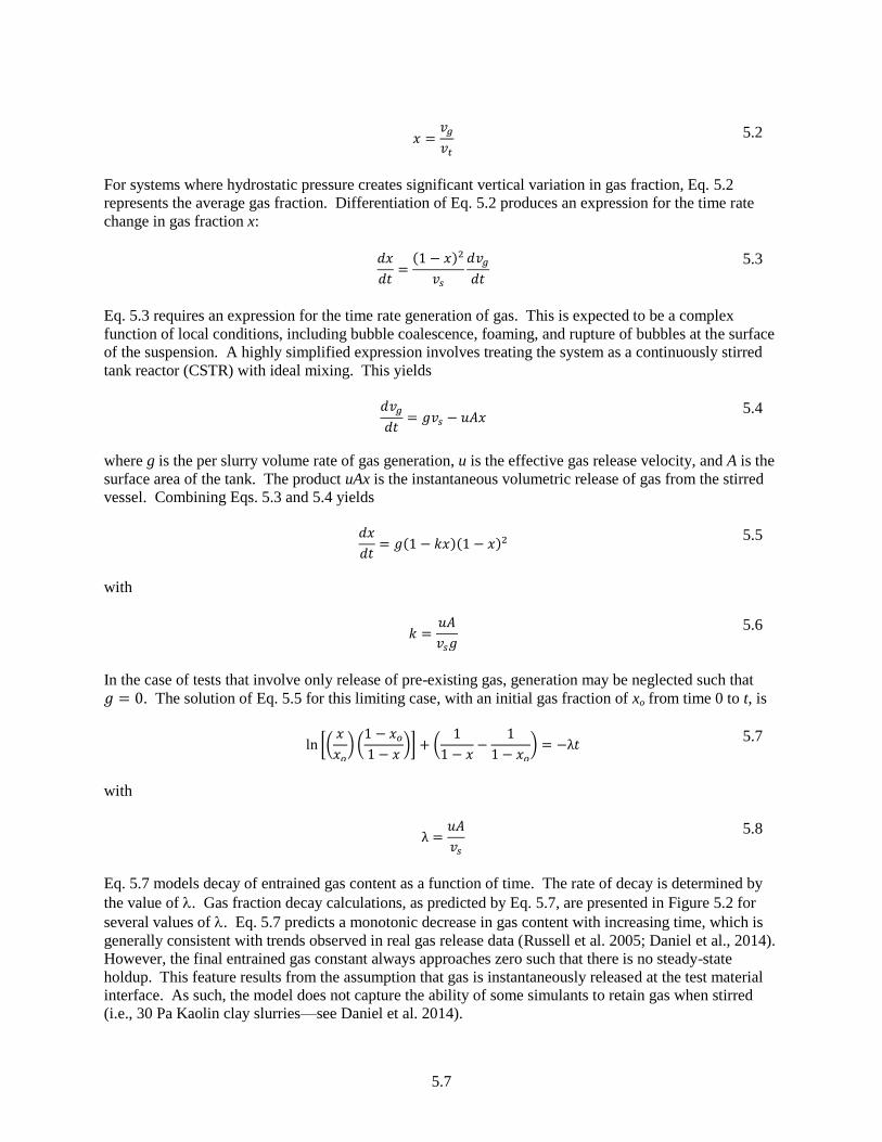
5.7
𝑥 =𝑣𝑔
𝑣𝑡
5.2
For systems where hydrostatic pressure creates significant vertical variation in gas fraction, Eq. 5.2
represents the average gas fraction. Differentiation of Eq. 5.2 produces an expression for the time rate
change in gas fraction x:
𝑑𝑥
𝑑𝑡=
(1 − 𝑥)2
𝑣𝑠
𝑑𝑣𝑔
𝑑𝑡
5.3
Eq. 5.3 requires an expression for the time rate generation of gas. This is expected to be a complex
function of local conditions, including bubble coalescence, foaming, and rupture of bubbles at the surface
of the suspension. A highly simplified expression involves treating the system as a continuously stirred
tank reactor (CSTR) with ideal mixing. This yields
𝑑𝑣𝑔
𝑑𝑡= 𝑔𝑣𝑠 − 𝑢𝐴𝑥
5.4
where g is the per slurry volume rate of gas generation, u is the effective gas release velocity, and A is the
surface area of the tank. The product uAx is the instantaneous volumetric release of gas from the stirred
vessel. Combining Eqs. 5.3 and 5.4 yields
𝑑𝑥
𝑑𝑡= 𝑔(1 − 𝑘𝑥)(1 − 𝑥)2
5.5
with
𝑘 =
𝑢𝐴
𝑣𝑠𝑔
5.6
In the case of tests that involve only release of pre-existing gas, generation may be neglected such that
𝑔 = 0. The solution of Eq. 5.5 for this limiting case, with an initial gas fraction of xo from time 0 to t, is
ln [(
𝑥
𝑥𝑜
) (1 − 𝑥𝑜
1 − 𝑥)] + (
1
1 − 𝑥−
1
1 − 𝑥𝑜
) = −λ𝑡 5.7
with
λ =
𝑢𝐴
𝑣𝑠
5.8
Eq. 5.7 models decay of entrained gas content as a function of time. The rate of decay is determined by
the value of . Gas fraction decay calculations, as predicted by Eq. 5.7, are presented in Figure 5.2 for
several values of . Eq. 5.7 predicts a monotonic decrease in gas content with increasing time, which is
generally consistent with trends observed in real gas release data (Russell et al. 2005; Daniel et al., 2014).
However, the final entrained gas constant always approaches zero such that there is no steady-state
holdup. This feature results from the assumption that gas is instantaneously released at the test material
interface. As such, the model does not capture the ability of some simulants to retain gas when stirred
(i.e., 30 Pa Kaolin clay slurries—see Daniel et al. 2014).

5.8
Figure 5.2. Sample calculations for gas release in the absence of generation. Calculations are based on
Eq. 5.7 with an initial entrained gas fraction (xo) of 0.3 and three values of (0.5, 1, and
2 min-1
). Note: This figure presents preliminary technical results for planning that should
not be used for WTP Design or Safety Analyses.
The general solution of Eq. 5.5, including gas generation, is given by
𝑘
(1 − 𝑘)2𝑙𝑛 [(
1 − 𝑥
1 − 𝑥𝑜
) (1 − 𝑘𝑥𝑜
1 − 𝑘𝑥)] + (
1
1 − 𝑘) (
1
1 − 𝑥−
1
1 − 𝑥𝑜
) = 𝑔𝑡 5.9
for 𝑘 ≠ 1 and
1
(1 − 𝑥)2−
1
(1 − 𝑥𝑜)2= 2𝑔𝑡
5.10
when 𝑘 = 1. Eqs. 5.9 and 5.10 predict the time rate change in the gas content during mixing. Gas
content can either monotonically increase or decrease depending on where the initial gas concentration
falls relative to its equilibrium value. At long times, the gas content approaches its equilibrium (or
steady-state) value (xe) where the rate of generation matches the rate of release. Here
𝑥𝑒 =
1
𝑘=
𝑔
𝜆
5.11
where 0 ≤ 𝑥𝑒 ≤ 1. Figure 5.3 shows the evolution of retained gas fraction as a function of time for
model systems with different xe (i.e., 0.1, 0.3, and 0.5). In physical terms, increased xe corresponds to
increased generation rate relative to the release rate. It should be noted that the steady-state holdup, per
Eq. 5.11, is expressed purely in terms of the generation rate (g) and the effective release rate (). This
means that, if the assumptions of this simple model hold, then steady-state holdup will be a linear
function of the generation rate, and can be calculated from experiments that assess only (i.e., static tests
where there is no generation).
0.00
0.05
0.10
0.15
0.20
0.25
0.30
0.35
0 5 10 15
Gas
Fra
ctio
n
Time (min)
= 2 min-1
= 1 min-1
= 0.5 min-1
Preliminary Technical Results for PlanningNot to be used for WTP Design or Safety Analyses

5.9
Figure 5.3. Sample calculations for gas release with generation. Calculations are based on Eq. 5.11 with
no initial entrained gas (xo = 0) and three equilibrium gas hold-up values (xe) of 0.1, 0.3, and
0.5. Note: This figure presents preliminary technical results for planning that should not be
used for WTP Design or Safety Analyses.
The model described on the previous pages, along with its governing equations, represents a simple first
order approximation for treating gas release. It captures basic features of transient gas generation, release,
and holdup. However, several important features expected in gas release behavior are not captured or
have been neglected, including the following:
the pressure dependence of gas fraction (increased hydrostatic head reduces gas fraction at increased
depth in the slurry)
the presence of transient flows, such as those encountered in systems mixed with PJMs, is not
captured but could be with a oscillatory release velocity (u)
model does not allow for peak holdup (i.e., a maximum in the retained gas fraction with time) nor
does it allow for non-zero steady-state holdup in the absence of gas generation
model assumes a constant gas release rate that is independent of retained gas fraction, though it is
plausible that the gas release rate may become smaller with decreasing gas fraction. Understanding
this dependence will likely be important for using static release test data (no generation during the
release) to predict steady-state hold up.
although captured implicitly in the release velocity (u), the model does not explicitly include fluid
physical properties (e.g., density, fluid yield stress, or fluid viscosity) that affect the rate of gas
release. This prevents application of modeling results to different fluids and different mixing
conditions.
In functional terms, the model is similar to a gas release model previously derived in Russell et al. (2005).
With respect to this previously derived model, the current model neglects effects of pressure (captured in
the prior model) but allows for analysis of release conditions with large entrained gas fractions (x > 0.1).
0.00
0.10
0.20
0.30
0.40
0.50
0.60
0 1 2 3 4 5
Gas
Fra
ctio
n
Time (min)
xe = 0.5
xe = 0.3
xe = 0.1
= 1 min-1 (for all)
Preliminary Technical Results for PlanningNot to be used for WTP Design or Safety Analyses

5.10
5.5 Preliminary Development and Characterization of Non-Newtonian Simulants for Gas Release Studies
The emphasis of this section is on non-Newtonian slurry simulants for gas retention and release tests
where there is no separation of solids from the liquid phase (no settling). The techniques discussed in this
section are also applicable, in general, to the relatively low-solids content simulants used in the settling
with gas retention and release studies that are described in more detail in Section 6.4.
One concept for comparing the gas release behaviors of various simulants is discussed previously in
Section 5.2 (see Figure 5.1). Another proposed method for comparatively evaluating gas retention and
release characteristics was tested on a preliminary basis. These preliminary tests, which used an air
sparger at low-flow rate in a 23 in. diameter vessel to induce gas release from a relatively large volume of
simulant, are discussed in Section 6.3. Section 6.3 also discusses a preliminary dead zone gas release test.
In support of these tests and the simulant selection activity in general, a number of non-Newtonian
simulants were prepared from kaolin and bentonite clays in varying proportions and in a range of solids
contents to target properties outlined in Table 5.1 of Section 5.2. Expecting that gas release
characteristics are a strong function of non-Newtonian rheological properties (e.g., shear strength, yield
stress, and consistency), these properties were measured and are compared extensively in Section 5.5.3.
For a small subset of non-Newtonian simulant samples, gas generation rate and settling were also
evaluated, and the results are discussed briefly (also in Section 5.5.3). First, simulant preparation
(Section 5.5.1) and characterization (Section 5.5.2) methods are described.
5.5.1 Simulant Preparation
Batches of simulant for characterization and/or preliminary gas release testing were prepared using
pre-defined recipes. For example, for simulant development and characterization, the solids content
would be varied with the goal of bracketing the range of properties of interest (e.g., shear strength or yield
stress). This provided information necessary to develop simple correlations from which recipes could be
defined to target specific simulant properties for other testing. This section summarizes the simulant
materials, the elements of a simulant recipe, and the standard methods of batch preparation (e.g., blending
and mixing) used to prepare both small quantities for simulant development and characterization and
larger volumes for gas release and mixing tests.
Acidified (pH-adjusted) 90:10 Min-U-Sil 30:Bentonite (M30:B) was used in limited testing described in
this report. M30:B simulant materials, recipes, and preparation methods were those used by Rassat et al.
(2014). Simulant development and characterization activities focused on K:B clay slurries.
5.5.1.1 Simulant Materials
The following materials were used in simulant preparation:
Kaolin (K) – EPK Pulverized kaolin clay from Edgar Minerals, Inc. (Edgar, Florida). The clay was
packaged as a dry powder in 50 lb bags, and used as-received (as-is). The expected moisture content
is ≤2 wt% based on previous analyses (e.g., Powell et al. 2014).
Bentonite (B) – Big Horn
BH 200 bentonite, previously sold as CH 200, supplied by Wyo-Ben, Inc.
Bentonite was packaged as a dry powder in 50 lb bags, and used as-received. Based on product
literature, the expected moisture content is 6 to 10 wt% and the specific gravity is 2.55.1
1 A May 2013 Rev. of a Technical Data Sheet for this grade of bentonite shows the noted typical moisture content
and a specific gravity of 2.55 ± 0.1.
5.11
Min-U-Sil
30 (M30) – Fine-ground crystalline silica produced by Brenntag Specialties, Inc. and
distributed by U.S. Silica. M30 was packaged as a dry powder in 50 lb bags, and used as-received.
Based on product literature, the expected moisture content is ≤0.5 wt% and the specific gravity is
2.65.1
Water – Richland City tap water was used as-is for simulant preparation unless otherwise noted.
Hydrochloric Acid (HCl) – 2.0 M HCl in water was used as-received in the preparation of a limited
number of slurry batches.2
Sodium chloride – Lab-grade or store-bought (e.g., Kosher) salt was dissolved in water prior to
addition of clay components. Typically, a 10 wt% solution having a handbook (CRC 2011) density
of 1.071 g/mL was used.
Hydrogen peroxide (H2O2) – Nominally 3 and 6 wt% H2O2 in water was supplied by Ricca Chemical
Company.3 The higher concentration solution was used primarily in some of the larger settling with
gas retention and release tests (Section 6.4).
Dye – A dye (e.g., blue) was added in low concentration to a portion of the simulant used in a dead
zone test (Section 6.3) to distinguish the dead zone from the bulk of the simulant. The dye was
dissolved in a small volume of water before mixing it in to the previously prepared stock slurry
simulant.
5.5.1.2 Simulant Recipes
Although simulant “formulation” and “recipe” are used somewhat interchangeably, they are formally
distinguished as follows. Simulant formulation defines the type of simulant in terms of the solid species
used, the relative weight fractions of the solid components (e.g., 80 percent kaolin and 20 percent
bentonite in 80:20 K:B) and any special modifications such as the use of NaCl solution instead of water
or acidification for pH adjustment. Unless otherwise noted, all simulant formulations were mixtures of
solids in unmodified tap water. Conversely, a recipe is the formulation and total concentration of solids.
Even more specifically, a recipe gives the type/grade/concentration and mass of each simulant component
needed to produce a target volume of simulant.
In gas release tests, a target final simulant solids concentration after H2O2 addition was specified.
Therefore, an initial pre-H2O2 slurry recipe at a higher solids concentration was developed anticipating the
amount of H2O2 that would be added. The higher concentration slurry was typically sampled for
characterization to extend the property vs. solids correlations. Small water-dilution samples with a water
mass proportionate to the amount of H2O2 to be added were, in many cases, also prepared from the test
stock slurry and characterized to obtain property information at the final simulant solids concentration.
1 An M30 Product Data Sheet issued October 2007 and revised December 2011 shows that it is typically 99.5
percent SiO2 and has a median particle size of 8.2 µm and a (particle) specific gravity of 2.65. 2 Because the HCl is used for gross adjustment of pH to approximate target values and not for analytical purposes, it
is not necessary to know the precise concentration (e.g., ±5% is acceptable). Label concentration of newly
purchased stock is sufficient. 3 The 4 L jugs of the nominally 3 wt% peroxide solution indicate that it has a Certified Traceable to NIST Standard
Reference Material Manufacturing Specification of 3.3 ± 0.1 wt% H2O2 (Cat. No. 3819-1) and that acetanilide is
used in small concentration as a stabilizer. Labels on the 20 L containers of 6 wt% solution, which we had no
previous experience using, did not provide information on concentration tolerances or stabilizers (if any). In any
case, certification of the concentration was not required for this testing.

5.12
5.5.1.3 Simulant Preparation
The preparation of simulant from defined recipes was similar for small and large batches except for the
containers and mixing equipment used. The differences are discussed below, following a summary of the
generally applicable steps.
The typical simulant batch preparation steps were:
1. Target simulant component masses were specified in recipes.
2. Actual masses of all components used in the batch were weighed and recorded, along with the
component concentrations and identifiers (e.g., lot numbers), where applicable.
3. If salt solution was used as the liquid phase, the salt was pre-dissolved in the specified amount of
water.
4. If more than one solids component (e.g., kaolin and bentonite) was used, the weighed solid materials
were premixed dry either by shaking (e.g., in a plastic container with a lid such as a 5 gal bucket) or
using mechanical agitators (e.g., the double-auger mixers described later in this section).
5. Solids were added slowly to the specified quantity of water (or salt solution, if applicable, but without
HCl and/or H2O2, if any) while operating the mechanical mixer. Mechanical mixing was typically
supplemented with manual mixing steps using spatulas and/or paddles to scrape the container walls
and corners. Depending on solids content, solids addition and mixing to a visually uniform
consistency typically took 5 to 10 minutes for ~15 L and smaller batches and up to a 30 minutes, but
typically less, for larger batches (e.g., ~140 L). For some batches, a standard or specified mixing time
after solids incorporation was used.
6. Once the water and solids were thoroughly mixed, mixing ceased and the hydration (or
“pre-hydration” for cases where acid was added) period started.
7. The prescribed amount of acid, if any, was added to the pre-hydrated slurry after a nominal pre-
hydration period of typically 4 ± 1 hour (following the practice of Rassat et al. (2014) for
90:10 M30:B simulant). The pre-hydrated slurry was remixed mechanically and the HCl solution was
added slowly while mixing. This step typically took 10 minutes or less.
8. The thoroughly mixed slurry was allowed to hydrate/equilibrate (with optional intermittent remixing)
for a specified duration. Batches were typically, but not always, allowed to hydrate overnight before
use in gas release testing. In general, a similar hydration period was used for simulant development
and characterization batches, but in a number of cases shorter and longer hydration periods were used
to assess possible effects of aging on properties.
9. After the prescribed hydration time and in preparation for acquisition of samples or the start of a test,
the batch was remixed. Depending on the batch size and consistency, this was typically done for 2 to
5 minutes using the original mixing method. Smaller batches (e.g., ≤1.5 L) of low-strength simulant
were sometimes remixed by hand.
10. Just prior to the start of a gas release test, the (portion of) slurry in which gas was to be generated was
remixed and the pre-weighed H2O2 solution was added while mechanically mixing, noting the time
that addition started. The slurry was mixed with H2O2 for ~5 minutes (or less in small batches), being
thorough while avoiding entrainment of air bubbles. To further reduce the amount of entrained air,
final mixing was done by hand with spatulas and/or paddles to dislodge larger bubbles.
As noted above, the primary difference in preparation of large (up to ~140 L), intermediate (e.g., 15 L)
and small (1 to 1.8 L) batches of simulant was the equipment used for mixing. Appropriately sized
cylindrical polymer tanks/drums were used for both dry blending, if any, and slurry mixing of large
5.13
batches. A double-auger mixer (i.e., Northern Industrial Tools Double Auger Mortar Mixer; 2 speed,
800 rpm maximum; 22 in. long shaft with ~6 in. long mixer paddle) was used for the slurry mixing steps
of large batches. For intermediate-sized batches prepared in 5 gal buckets, only one of the two included
mixing paddles was used (i.e., effectively a single-auger mixer, but the term “double-auger” is commonly
retained). Alternatively, a paint-mixer paddle mounted in a battery-powered drill motor was used to mix
5 gal bucket batches or larger batches of low-solids slurry. The smallest batches were prepared using a
KitchenAid® stand mixer with the supplied steel bowl and mixing paddle. Its adjustable speed control
was usually set to ~“2” and typically run for ~10 minutes after solids were well incorporated at Speed
~”1.”
5.5.2 Simulant Characterization
Section 5.5.2.1 describes the analytical methods used for characterization of simulant physical and
chemical properties; Section 5.5.2.2 provides an outline of methods used for analysis and interpretation of
simulant property data.
5.5.2.1 Analytical Methods
The key properties of slurry simulants used in preliminary tests were characterized following the
RPL-COLLOID-02 procedure.1 The following methods were selectively applied to determine the
physical (i.e., density and rheology) and chemical (i.e., pH) properties of ~500 mL (typical) samples of
slurry simulants. Slurry batches were generally allowed to hydrate for a minimum of 4 hours after
preparation, and often overnight, before rheological properties were measured.
Density – The bulk simulant density, S, was determined by measuring the mass and volume of a
sample placed in commercial off-the-shelf 500 mL or 1 L graduated cylinder. Masses were obtained
using balances having ±0.1 g or greater precision (e.g., Sartorius model CP 34001 S). The
measurement method and equipment were selected to give a standard density measurement accuracy
of ±2 percent (and typically less than ±1 percent).
pH – The pH of slurries and supernatant liquids was measured using a pH meter that was
user-calibrated to ±0.1 pH unit (or less) and performance-checked using certified pH buffer solutions.
The pH electrode was directly immersed in the liquid or freshly mixed slurry.
Shear Strength – The shear strength, S, was determined by the shear vane method using a Thermo
Fisher Scientific HAAKE Viscotester 550. Using the instrument in a rotational viscometer
configuration with certified viscosity standards, the performance was checked to be within
±10 percent accuracy. For shear strength measurements, the instrument torque resolution
(uncertainty) was ±0.5 percent of the 30 mN·m range. The shear vane used has a cross-pattern
(viewed from the end) and is 16 mm diameter 32 mm height. It was set to rotational rate of 0.3 rpm
for measurements. Shear strength was determined from the peak torque recorded by the instrument
software and the vane geometry. The shear strength was measured on thoroughly mixed samples that
were typically allowed to stand undisturbed for ~1 hour. Replicate measurements, if any, were made
1 The analytical simulant characterization data were obtained following the guidelines of the most current version of
RPL-COLLOID-02 by RC Daniel, “Measurement of Physical and Rheological Properties of Solutions, Slurries, and
Sludges.” The current Revision Number is 2, effective March 11, 2011. When fully implemented under a
governing QA program at the Applied Research (or higher) grade, data obtained under RPL-COLLOID-02 and
documented and reviewed following applicable QA Procedures can be NQA-1 qualified. However, the simulants
discussed in this report were prepared and characterized at the Basic Research level, and the data are, therefore, FIO.
5.14
in undisturbed material located at least 2 vane diameters away from other measurement locations. In
some noted cases, slurry was allowed to stand undisturbed for some duration other than ~1 hour prior
to measurement.
Rheology – Non-Newtonian simulant rheology was further characterized by obtaining rheograms
using an Anton-Paar Physica MCR301 rotational viscometer using a concentric cylinder sample
geometry. The instrument performance was verified to be within ±10 percent accuracy using certified
viscosity standards. Using software provided with the instrument, the data were fit to a two-
parameter Bingham plastic model (e.g., defined by a yield stress, 0, and a consistency [viscosity at
infinite shear rate], μ∞). Samples were premixed by hand just prior to loading the sample cell and
were pre-sheared by the instrument for 3 minutes at a shear rate of 250 s-1
immediately before
recording the rheograms. Typically, two consecutive rheograms (i.e., runs) were obtained by ramping
the shear rate up and down in the range of 0 to 1000 s-1
in each cycle, and Bingham model parameters
(see Section 5.5.2.2) were determined by using the rheometer software to fit a line to the data of the
second down ramp in the range of 200 to 800 s-1
.1 Bingham parameters were determined from second
up-ramp data for comparison to the down-ramp results in some noted cases (Section 5.5.3.2).
Selected analyses above were most often applied to as-prepared simulant samples. In some cases, small
portions of slurry batches were diluted with water and thoroughly mixed2 to achieve a target solids
concentration (xS) for additional analyses. This approach was used, for example, to generate small
water-dilution samples having the same final solids content as the large slurry batch following the
addition of H2O2. Creating these water-dilution samples with a proportionate amount of water overcomes
analytical challenges due to extended generation and retention of oxygen gas associated with H2O2
decomposition in the actual test batch.
The density method noted above is also applicable to settling studies in non-Newtonian and low-solids
simulant samples (Section 5.5.3.4 and Section 6.4, respectively) and graduated cylinder gas retention and
release experiments (e.g., Section 5.5.3.3). Along with simulant composition information and (initial)
mass, tracking overall and settled-solids layer (if any) volumes vs. time allows for the determination of
changes in bulk density and/or settled layer density and estimate retained gas volumes. Mass loss due to
release of oxygen bubbles generated from H2O2 decomposition, if any, is negligible. Changes in mass
due to evaporation over the course of the reported tests were not typically measured and were assumed to
be negligible for the purpose of these preliminary assessments.
5.5.2.2 Methods of Simulant Property Data Analysis and Interpretation
Slurry density, shear strength, and rheology (e.g., Bingham model parameters) are a function of the
simulant composition and the solids concentration. Methods of correlating and interpreting the
relationship between these properties and total solids content are described below.
Theoretical Density
Analogous to methods used previously for clay simulants, a theoretical slurry density (S) can be
estimated from the relative weight fractions (fi) of solid species i, the total weight fraction of solids in the
slurry (xS), and the solid and liquid component densities (obtained from references)
1 Alternate total shear rate and fitting ranges were applied in a limited number of noted cases.
2 Small, beaker-sized samples were typically mixed by hand with a spatula. For dilution of larger quantities of
slurry, a mechanical mixing method applicable to the size of the batch was used (see Section 5.5.1).
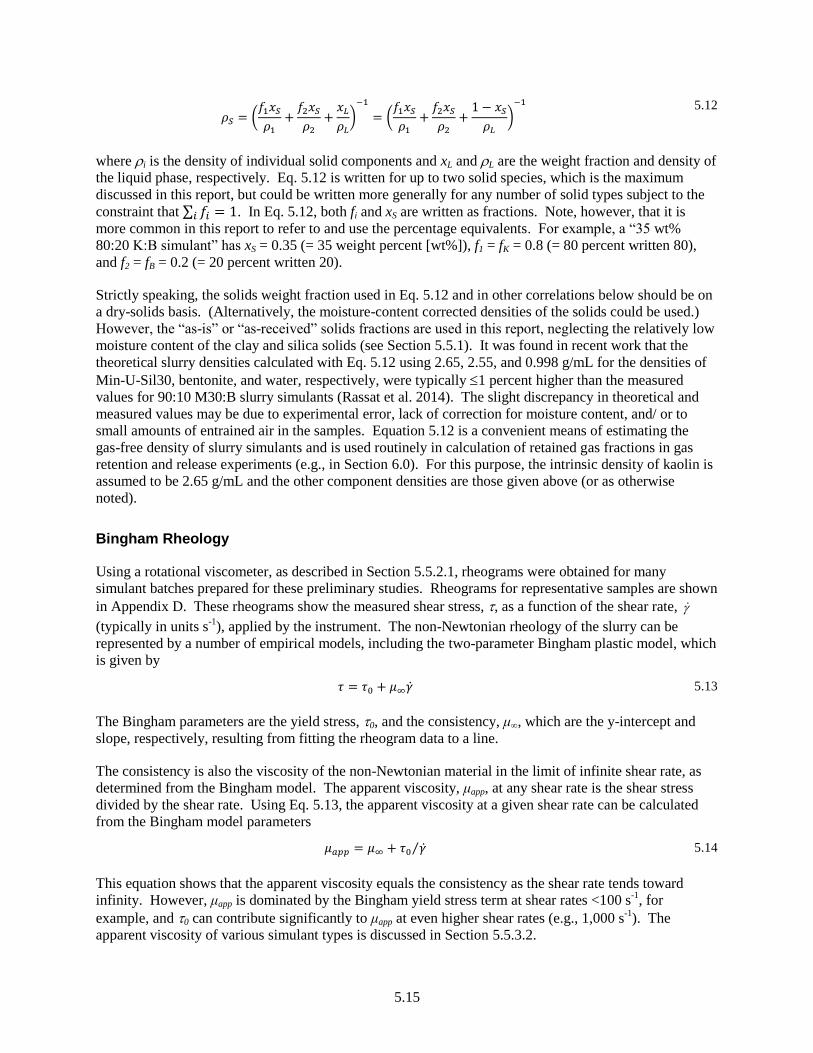
5.15
𝜌𝑆 = (
𝑓1𝑥𝑆
𝜌1
+𝑓2𝑥𝑆
𝜌2
+𝑥𝐿
𝜌𝐿
)−1
= (𝑓1𝑥𝑆
𝜌1
+𝑓2𝑥𝑆
𝜌2
+1 − 𝑥𝑆
𝜌𝐿
)−1
5.12
where i is the density of individual solid components and xL and L are the weight fraction and density of
the liquid phase, respectively. Eq. 5.12 is written for up to two solid species, which is the maximum
discussed in this report, but could be written more generally for any number of solid types subject to the
constraint that ∑ 𝑓𝑖𝑖 = 1. In Eq. 5.12, both fi and xS are written as fractions. Note, however, that it is
more common in this report to refer to and use the percentage equivalents. For example, a “35 wt%
80:20 K:B simulant” has xS = 0.35 (= 35 weight percent [wt%]), f1 = fK = 0.8 (= 80 percent written 80),
and f2 = fB = 0.2 (= 20 percent written 20).
Strictly speaking, the solids weight fraction used in Eq. 5.12 and in other correlations below should be on
a dry-solids basis. (Alternatively, the moisture-content corrected densities of the solids could be used.)
However, the “as-is” or “as-received” solids fractions are used in this report, neglecting the relatively low
moisture content of the clay and silica solids (see Section 5.5.1). It was found in recent work that the
theoretical slurry densities calculated with Eq. 5.12 using 2.65, 2.55, and 0.998 g/mL for the densities of
Min-U-Sil30, bentonite, and water, respectively, were typically 1 percent higher than the measured
values for 90:10 M30:B slurry simulants (Rassat et al. 2014). The slight discrepancy in theoretical and
measured values may be due to experimental error, lack of correction for moisture content, and/ or to
small amounts of entrained air in the samples. Equation 5.12 is a convenient means of estimating the
gas-free density of slurry simulants and is used routinely in calculation of retained gas fractions in gas
retention and release experiments (e.g., in Section 6.0). For this purpose, the intrinsic density of kaolin is
assumed to be 2.65 g/mL and the other component densities are those given above (or as otherwise
noted).
Bingham Rheology
Using a rotational viscometer, as described in Section 5.5.2.1, rheograms were obtained for many
simulant batches prepared for these preliminary studies. Rheograms for representative samples are shown
in Appendix D. These rheograms show the measured shear stress, , as a function of the shear rate,
(typically in units s-1
), applied by the instrument. The non-Newtonian rheology of the slurry can be
represented by a number of empirical models, including the two-parameter Bingham plastic model, which
is given by
𝜏 = 𝜏0 + 𝜇∞�̇� 5.13
The Bingham parameters are the yield stress, 0, and the consistency, μ∞, which are the y-intercept and
slope, respectively, resulting from fitting the rheogram data to a line.
The consistency is also the viscosity of the non-Newtonian material in the limit of infinite shear rate, as
determined from the Bingham model. The apparent viscosity, μapp, at any shear rate is the shear stress
divided by the shear rate. Using Eq. 5.13, the apparent viscosity at a given shear rate can be calculated
from the Bingham model parameters
𝜇𝑎𝑝𝑝 = 𝜇∞ + 𝜏0 �̇�⁄ 5.14
This equation shows that the apparent viscosity equals the consistency as the shear rate tends toward
infinity. However, μapp is dominated by the Bingham yield stress term at shear rates <100 s-1
, for
example, and 0 can contribute significantly to μapp at even higher shear rates (e.g., 1,000 s-1
). The
apparent viscosity of various simulant types is discussed in Section 5.5.3.2.

5.16
Correlations for Rheological Properties and Solids Content
As shown in the next section (Section 5.5.3), slurry simulant shear strength, Bingham yield stress, and
Bingham consistency can each be well correlated to solids content by fitting respective data to
exponential functions of the form
𝑦 = 𝐴𝑒𝑐𝑒𝑥𝑆 5.15
where the solids fraction xS is typically expressed in weight % and A and ce are the fit pre-exponential and
exponential constants, respectively. Such correlations allow interpolation or extrapolation to target
parameter values for determining simulant recipes (e.g., solids content) or for comparison of different
simulant types at a standard basis, for example. This approach is used in Section 5.5.3.2 to compare the
apparent viscosity of simulants at constant yield stress (15 or 30 Pa) as follows: a) using previously
determined exponential fit constants for 0 vs. solids content, Eq. 5.15 is inverted and solved for xS at the
target yield stress; b) xS is then used along with previously determined exponential fit constants for μ∞ vs.
solids content to determine the corresponding consistency; and c) finally, the specified 0 and solved for
μ∞ are used in Eq. 5.14 to determine μapp as a function of shear rate.
5.5.3 Non-Newtonian Simulant Properties (Non-Settling)
In an effort to identify non-Newtonian simulants exhibiting a range of gas release behavior for use in
preliminary gas release studies, several K:B clay simulant formulations were evaluated. For each
simulant type (e.g., K:B weight ratio), at least two batches at different solids concentration were prepared
and characterized to better be able to target physical properties of simulants and provide specific recipes
for gas release studies. This section summarizes the key properties of the K:B simulants and, in some
cases, compares them to other simulants reported in the literature. The rheology of K:B simulants is
emphasized, starting with a discussion of the shear strength of 100 percent kaolin slurry and shifting to a
more general discussion and comparison of rheological characteristics of the various simulant
formulations. The use of pH adjustment in 80:20 K:B simulant to reduce the gas generation rate resulting
from hydrogen peroxide decomposition is then briefly demonstrated. Finally, a limited evaluation of
settling characteristics of some (preferably) “non-settling” non-Newtonian K:B simulants is touched on.
5.5.3.1 Kaolin Simulant Shear Strength
In preparation for a kaolin simulant gas release test discussed in Section 6.3, three 1 L KitchenAid
batches of kaolin in water simulant in the range of 35 to 43 wt% solids were made1 and shear strengths
were measured. This was done to develop a τS vs. xS correlation using the stock of kaolin on-hand,
especially for relatively weak formulations (e.g., ≤ 30 Pa yield stress and/or shear strength) for which
limited data exist, and because of known variability in shear strength correlations for EPK kaolin (e.g.,
Burns et al. 2010). The new small-batch correlation indicated that ~43 wt% kaolin was necessary to
reach the target shear strength of ~20 Pa. Subsequent preparation of ~120 L of 48.9 wt% kaolin slurry
and a water-dilution sample from it at the final 43 wt% solids target showed that the shear strength was
about twice that expected (i.e., ~40 Pa). A second water-dilution sample at 39 wt% solids hit the target
20 Pa shear strength and was eventually used in 23 in. vessel testing.
1 Unless otherwise noted, the default standard mixing protocol in the KitchenAid mixer was ~10 minutes at a
relatively low speed following completion of solids addition to water. In the kaolin-water batches discussed in this
section, the default was Speed 1. Due in part to the results of this section, the higher, but still relatively low, Speed
2 was chosen as the standard for later studies of kaolin:bentonite slurry batch properties (e.g., Section 5.5.3.2).
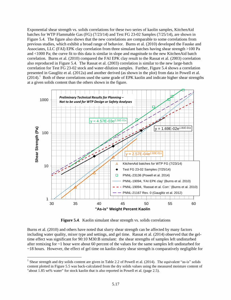
5.17
Exponential shear strength vs. solids correlations for these two series of kaolin samples, KitchenAid
batches for WTP Flammable Gas (FG) (7/23/14) and Test FG 23-02 Samples (7/25/14), are shown in
Figure 5.4. The figure also shows that the new correlations are comparable to some correlations from
previous studies, which exhibit a broad range of behavior. Burns et al. (2010) developed the Fauske and
Associates, LLC (FAI) EPK clay correlation from three simulant batches having shear strength >100 Pa
and <1000 Pa; the curve fit to this data is similar in slope and magnitude to the new KitchenAid batch
correlation. Burns et al. (2010) compared the FAI EPK clay result to the Rassat et al. (2003) correlation
also reproduced in Figure 5.4. The Rassat et al. (2003) correlation is similar to the new large-batch
correlation for Test FG 23-02 stock and water-dilution samples. Further, Figure 5.4 shows a correlation
presented in Gauglitz et al. (2012a) and another derived (as shown in the plot) from data in Powell et al.
(2014).1 Both of these correlations used the same grade of EPK kaolin and indicate higher shear strengths
at a given solids content than the others shown in the figure.
Figure 5.4. Kaolin simulant shear strength vs. solids correlations
Burns et al. (2010) and others have noted that slurry shear strength can be affected by many factors
including water quality, mixer type and settings, and gel time. Rassat et al. (2014) observed that the gel-
time effect was significant for 90:10 M30:B simulant: the shear strengths of samples left undisturbed
after remixing for ~1 hour were about 60 percent of the values for the same samples left undisturbed for
~18 hours. However, the effect of gel time on kaolin slurry shear strength is comparatively negligible for
1 Shear strength and dry solids content are given in Table 2.2 of Powell et al. (2014). The equivalent “as-is” solids
content plotted in Figure 5.5 was back-calculated from the dry solids values using the measured moisture content of
"about 1.85 wt% water" for stock kaolin that is also reported in Powell et al. (page 2.5).
y = 2.57E-04e2.60E-01x
y = 1.69E-02e1.81E-01x
y = 4.57E-03e2.26E-01x
1
10
100
1000
30 35 40 45 50 55 60
Sh
ea
r S
tren
gth
(P
a)
"As-is" Weight Percent Kaolin
KitchenAid batches for WTP FG (7/23/14)
Test FG 23-02 Samples (7/25/14)
PNNL-23136 (Powell et al. 2014)
PNNL-19094, 'FAI EPK clay' (Burns et al. 2010)
PNNL-19094, 'Rassat et al. Corr.' (Burns et al. 2010)
PNNL-21167 Rev. 0 (Gauglitz et al. 2012)
Preliminary Technical Results for Planning –Not to be used for WTP Design or Safety Analyses
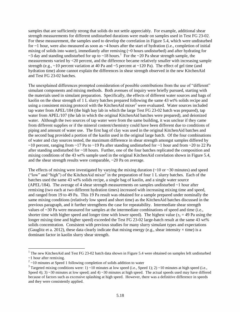
5.18
samples that are sufficiently strong that solids do not settle appreciably. For example, additional shear
strength measurements for different undisturbed durations were made on samples used in Test FG 23-02.
For these measurement, the samples used to develop the correlation in Figure 5.4, which were undisturbed
for ~1 hour, were also measured as soon as ~4 hours after the start of hydration (i.e., completion of initial
mixing of solids into water), immediately after remixing (~0 hours undisturbed) and after hydrating for
~3 day and standing undisturbed for up to ~18 hours.1 For the ~20 Pa shear strength sample, the
measurements varied by <20 percent, and the difference became relatively smaller with increasing sample
strength (e.g., ~10 percent variation at 40 Pa and ~5 percent at ~120 Pa). The effect of gel time (and
hydration time) alone cannot explain the differences in shear strength observed in the new KitchenAid
and Test FG 23-02 batches.
The unexplained differences prompted consideration of possible contributions from the use of “different”
simulant components and mixing methods. Both avenues of inquiry were briefly pursued, starting with
the materials used in simulant preparation. Specifically, the effects of different water sources and bags of
kaolin on the shear strength of 1 L slurry batches prepared following the same 43 wt% solids recipe and
using a consistent mixing protocol with the KitchenAid mixer2 were evaluated. Water sources included
tap water from APEL/184 (the high bay lab in which the large Test FG 23-02 batch was prepared), tap
water from APEL/107 (the lab in which the original KitchenAid batches were prepared), and deionized
water. Although the two sources of tap water were from the same building, it was unclear if they came
from different supplies or if the mineral content/chemistry could have been different due to conditions of
piping and amount of water use. The first bag of clay was used in the original KitchenAid batches and
the second bag provided a portion of the kaolin used in the original large batch. Of the four combinations
of water and clay sources tested, the maximum difference in shear strength amongst samples differed by
~10 percent, ranging from ~17 Pa to ~19 Pa after standing undisturbed for ~1 hour and from ~20 to 22 Pa
after standing undisturbed for ~18 hours. Further, one of the four batches replicated the composition and
mixing conditions of the 43 wt% sample used in the original KitchenAid correlation shown in Figure 5.4,
and the shear strength results were comparable, ~20 Pa on average.
The effects of mixing were investigated by varying the mixing duration (~10 or ~30 minutes) and speed
(“low” and “high”) of the KitchenAid mixer3 in the preparation of four 1 L slurry batches. Each of the
batches used the same 43 wt% solids recipe, a single bag of kaolin, and a single water source
(APEL/184). The average of 4 shear strength measurements on samples undisturbed ~1 hour after
remixing (two each at two different hydration times) increased with increasing mixing time and speed,
and ranged from 19 to 49 Pa. This 19 Pa result was obtained for a sample prepared under nominally the
same mixing conditions (relatively low speed and short time) as the KitchenAid batches discussed in the
previous paragraph, and it further strengthens the case for repeatability. Intermediate shear strength
values of ~30 Pa were measured for samples at the intermediate combinations of speed and time (i.e.,
shorter time with higher speed and longer time with lower speed). The highest value (τS = 49 Pa using the
longer mixing time and higher speed) exceeded the Test FG 23-02 large-batch result at the same 43 wt%
solids concentration. Consistent with previous studies for many slurry simulant types and expectations
(Gauglitz et a. 2012), these data clearly indicate that mixing energy (e.g., shear intensity × time) is a
dominant factor in kaolin slurry shear strength.
1 The new KitchenAid and Test FG 23-02 batch data shown in Figure 5.4 were obtained on samples left undisturbed
~1 hour after remixing. 2 ~10 minutes at Speed 1 following completion of solids addition to water
3 Targeted mixing conditions were: 1) ~10 minutes at low speed (i.e., Speed 1); 2) ~10 minutes at high speed (i.e.,
Speed 4); 3) ~30 minutes at low speed; and 4) ~30 minutes at high speed. The actual speeds used may have differed
because of factors such as excessive splashing at high speed. However, there was a definitive difference in speeds
and they were consistently applied.

5.19
5.5.3.2 Rheology of Kaolin:Bentonite Simulants
Available shear strength and Bingham parameter data along with formulation information are tabulated in
Appendix D for the non-Newtonian simulants discussed in Section 5.5.3 and for simulants used in
preliminary spontaneous and induced gas release tests (Section 6.3).
This section addresses initial non-Newtonian simulant development and characterization activities that
were completed in support of preliminary and anticipated gas retention and release studies. In limited
bench-scale testing to compare the gas release behavior of a few simulant types to that of Hanford
241-SY-101 DST waste (in historic video), Rassat et al. (2014) observed notable differences in the gas
release characteristics of pure bentonite, pure kaolin, and 90:10 Min-U-Sil30:bentonite slurry simulants,
with a tendency for gas to be less readily released from kaolin slurry. As noted in Section 5.2, 80:20 K:B
simulants have often been used in WTP-related gas retention and release testing. In keeping with the
historic use of K:B simulants in WTP gas release testing and in the interest of identifying a conservative1
but representative simulant that also satisfies targets and requirements shown in Table 5.1 (Section 5.2),
K:B simulants with solids ratios in the range of 80:20 to 100:0 (pure kaolin) were investigated. Bentonite
fractions > 20 percent result in simulants that tend to be too low in density and generate gas too quickly
via H2O2 decomposition.
Pure kaolin slurry (100:0 K:B) represents one potential extreme in gas release characteristics, which are
expected to be a function of rheological properties. The rheology of the kaolin slurry samples prepared in
the mixing study described in the last paragraph of Section 5.5.3.1 (and tabulated in Appendix D) was
unexpected in the following ways. First, for four batches that were expected to have nearly identical
properties based on their identical recipes (i.e., 43 wt% kaolin), the shear strength varied by a factor of
approximately 2.5 (τS = 19 to 49 Pa) while the Bingham yield stress and consistency were essentially
constant: τ0 ranged from 230 to 239 Pa and μ∞ ranged from 75 to 83 mPa·s (cP). This may not be overly
surprising considering that all samples were equally pre-sheared in the viscometer prior to obtaining
rheograms. It is possible that this further shearing in the viscometer sample cell was sufficient to give
equivalent slurry structure and physical properties while the subsamples for shear strength measurements
had different shear histories. The fact that the rheological properties of kaolin slurry are a function of
shear history is a topic of further discussion below.
Another noteworthy finding for the 100 percent kaolin simulants is that the yield stress, determined by a
dynamic method on continuously sheared samples, significantly exceeded the shear strength of samples
that were held static (undisturbed) and allowed to develop structure for ~1 hour or more. The ratio of
“strength” terms τ0/τS ranged from ~5 to >10 (or equivalently, τS/τ0 = 0.08 to 0.21, shear strength < yield
stress) for the kaolin mixing study samples. Again, this may be indicative of shearing effects in the
viscometer being more dominant than in initial mixing. A somewhat concerning aspect of these results is
that to achieve target yield stresses of 3 to 30 Pa, the kaolin solids content would be sufficiently low that
settling of solids could be significant, which is undesirable in non-Newtonian simulant testing, and the
shear strength would be exceedingly weak.
It is common in WTP vernacular to refer to 80:20 K:B formulations as “30/30” or “6/6”, indicating that
the magnitudes of the yield stress in Pa and the consistency in cP are equal. Similarly, see the equal
magnitude bounding targets of yield stress and consistency in Table 5.1 in Section 5.2. In addition,
1 In this context, conservative generally means that it is harder to release gas from the simulant. For example, higher
gas holdup in a continually mixed system would be expected with a conservative simulant. On the other hand, if
one were attempting to bound maximum gas release rates in an off-normal event by measurement (rather than
assume instantaneous, for example), a simulant that retained significant quantities of gas and released it readily once
disturbed would be conservative.

5.20
80:20 K:B simulant is typically treated as having shear strength greater than the yield stress by about a
factor of 2 (e.g., τS/τ0 = 60 Pa/30 Pa = 2). These expected rheological characteristics trace back to early
selection and use of a simulant for WTP PJM mixing studies (e.g., Poloski et al. 2004). As noted
previously, 100:0 K:B slurry does not meet these typical rheological property relationships, having shear
strength significantly lower than the yield stress and yield stress greater in magnitude than the consistency
by about a factor of 3 (e.g., ~230 Pa/~80 cP). Attempts were made to move the rheological characteristics
of pure kaolin toward the “norm” by adding bentonite, which is known to achieve relatively high
(cohesive) strength at low-solids concentration. Bentonite addition was also considered to have other
potential benefits, including decreasing the tendency for gravity settling of weak kaolin slurries and
increasing gas generation rates with H2O2, which tend to be slow (from an experimental perspective) with
kaolin alone. Newly tested formulations included 98:2 K:B, 95:5 K:B, and 90:10 K:B.
Two to three 1.5 L batches of each simulant composition at varying solids concentrations were prepared
using the KitchenAid mixer.1 The goal was to define simulant recipes that would be in the ~3 to ~30 Pa
strength range (either τS or τ0), but this was done without the foreknowledge of strength-to-solids
correlations so the target was often missed for these preliminary tests. Figure 5.5 shows in individual
plots the shear strength and Bingham yield stress and consistency (from standard rheogram down-ramp
fits) as a function of solids content for 80:20 to 100:0 K:B in water simulants. Each data set includes
exponential trend lines that are extrapolated beyond the range of data to facilitate comparison of the
various simulant types at constant property values. The coefficients of the exponential curve fits (see
Eq. 5.15 in Section 5.5.2.2) are tabulated in Appendix D for reference. The data shown in Figure 5.5 are
from KitchenAid batches except for 100 percent kaolin, which was taken from samples of large batches
and for which both shear strength and Bingham parameter data over a range of solids content were
available. The shear strength from the highest kaolin solids sample (48.9 wt%) is shared with Figure 5.4
(Section 5.5.3.1); however, the additional lower-solids data in Figure 5.5 was obtained from samples of a
second large batch. Although it was demonstrated in the previous section that the mixing method has an
effect on kaolin slurry shear strength, it is worthwhile to include 100:0 K:B data in the current analysis for
comparison. The overall, generalized trend is for decreasing solids content with increasing bentonite
fraction to achieve a given constant property value of τS, τ0, or μ∞, as expected. However, the trend is not
universal, and is particularly apparent for the 98:2 K:B and 100:0 K:B formulations when compared to
formulations with higher bentonite content. Given the limited data (e.g., only two batches of 98:2 K:B), it
remains unclear whether the deviation from the general trend is actual or anomalous (e.g., due to
batch-to-batch variation and/or differences in mixing methods).
Figure 5.5 also includes data for an 80:20 K:B simulant adjusted to pH 4 to 5 with hydrochloric acid and
95:5 K:B slurry prepared in 10 wt% NaCl/water solution instead of pure water. The former was done
primarily to reduce the gas generation rate compared to standard 80:20 K:B (see Section 5.5.3.3). The
95:5 K:B in salt formulation was investigated as a possible means to increase the overall simulant density
and increase the supernatant liquid density should solids separation occur (or an equivalent supernatant
layer be intentionally added in gas retention and release testing). Compared to their respective standard
formulations in water, both modified forms consistently show increased rheological property values for a
given solids content. In both cases, this may be attributed to increased cohesive interactions of clay
particles, though the specific mechanism has not been determined.
For the purpose of comparing shear strength to yield stress and yield stress to consistency of each
simulant type, it is useful to look directly at ratio data than to determine it from the individual property
plots in Figure 5.5. Thus, Figure 5.6 provides the ratio data for τS/τ0 and τ0/μ∞ as a function of shear
strength. Yield stress could similarly be used for the x-axis values, at the expense of widening the data
1 A standard mixing protocol of ~10 minutes at Speed 2 following completion of solids addition to water at Speed 1
was adopted for these “later” batches (compared to the “earlier” kaolin-water batches discussed in Section 5.5.3.1).
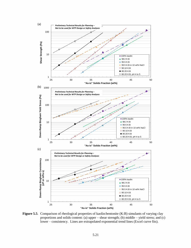
5.21
Figure 5.5. Comparison of rheological properties of kaolin:bentonite (K:B) simulants of varying clay
proportions and solids content: (a) upper – shear strength; (b) middle – yield stress; and (c)
lower – consistency. Lines are extrapolated exponential trend lines (Excel curve fits).
1
10
100
25 30 35 40 45 50
Sh
ea
r S
tren
gth
(P
a)
"As-is" Solids Fraction (wt%)
100% kaolin
98:2 K:B
95:5 K:B
95:5 K:B in 10 wt% NaCl
90:10 K:B
80:20 K:B
80:20 K:B, pH 4 to 5
Preliminary Technical Results for Planning –Not to be used for WTP Design or Safety Analyses
(a)
1
10
100
1000
25 30 35 40 45 50
Do
wn
-Ra
mp
Bin
gh
am
Yie
ld S
res
s (
Pa
)
"As-is" Solids Fraction (wt%)
100% kaolin
98:2 K:B
95:5 K:B
95:5 K:B in 10 wt% NaCl
90:10 K:B
80:20 K:B
80:20 K:B, pH 4 to 5
Preliminary Technical Results for Planning –Not to be used for WTP Design or Safety Analyses
(b)
1
10
100
25 30 35 40 45 50
Do
wn
-Ra
mp
Bin
gh
am
Co
ns
iste
nc
y(c
P o
r m
Pa
·s)
"As-is" Solids Fraction (wt%)
100% kaolin
98:2 K:B
95:5 K:B
95:5 K:B in 10 wt% NaCl
90:10 K:B
80:20 K:B
80:20 K:B, pH 4 to 5
Preliminary Technical Results for Planning –Not to be used for WTP Design or Safety Analyses
(c)

5.22
Figure 5.6. Comparison of rheological property ratios of K:B simulants of varying clay proportions and
solids content as a function of shear strength: (a) upper – shear strength/yield stress and
(b) lower – yield stress/consistency
0
0.2
0.4
0.6
0.8
1
1.2
1.4
1.6
1.8
2
0 20 40 60 80 100 120
Sh
ea
r S
tren
gth
/ Y
ield
Str
es
s
Shear Strength (Pa)
100% kaolin
98:2 K:B
95:5 K:B
95:5 K:B in 10 wt% NaCl
90:10 K:B
80:20 K:B
80:20 K:B, pH 4 to 5
Preliminary Technical Results for Planning –Not to be used for WTP Design or Safety Analyses
(a)
0
0.5
1
1.5
2
2.5
3
3.5
4
0 20 40 60 80 100 120
Yie
ld S
tres
s / C
on
sis
ten
cy
(Pa
/mP
a·s
or
Pa
/cP
)
Shear Strength (Pa)
100% kaolin
98:2 K:B
95:5 K:B
95:5 K:B in 10 wt% NaCl
90:10 K:B
80:20 K:B
80:20 K:B, pH 4 to 5
Preliminary Technical Results for Planning –Not to be used for WTP Design or Safety Analyses
(b)
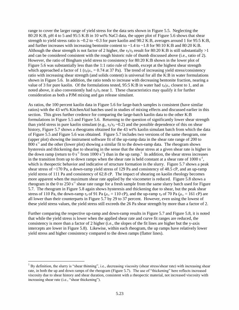
5.23
range to cover the larger range of yield stress for the data sets shown in Figure 5.5. Neglecting the
80:20 K:B, pH 4 to 5 and 95:5 K:B in 10 wt% NaCl data, the upper plot of Figure 5.6 shows that shear
strength to yield stress ratio is ~0.2 to ~0.3 for pure kaolin and 98:2 K:B, averages around 1 for 95:5 K:B,
and further increases with increasing bentonite content to ~1.4 to ~1.8 for 90:10 K:B and 80:20 K:B.
Although the shear strength is not factor of 2 higher, the τS/τ0 result for 80:20 K:B is still substantially >1
and can be considered consistent with the rough historic rule of thumb discussed above (i.e., ratio of 2).
However, the ratio of Bingham yield stress to consistency for 80:20 K:B shown in the lower plot of
Figure 5.6 was substantially less than the 1:1 ratio rule of thumb, except at the highest shear strength
which approached a factor of 1 (τ0/μ∞ = 0.74 at 37 Pa). The trend of increasing yield stress/consistency
ratio with increasing shear strength (and solids content) is universal for all the K:B in water formulations
shown in Figure 5.6. In addition, the ratio tends to increase with decreasing bentonite fraction, nearing a
value of 3 for pure kaolin. Of the formulations tested, 95:5 K:B in water had τ0/μ∞ closest to 1, and as
noted above, it also conveniently had τS/τ0 near 1. These characteristics may qualify it for further
consideration as both a PJM mixing and gas release simulant.
As ratios, the 100 percent kaolin data in Figure 5.6 for large-batch samples is consistent (have similar
ratios) with the 43 wt% KitchenAid batches used in studies of mixing effects and discussed earlier in this
section. This gives further credence for comparing the large-batch kaolin data to the other K:B
formulations in Figure 5.5 and Figure 5.6. Returning to the question of significantly lower shear strength
than yield stress in pure kaolin simulant (e.g., τS/τ0 ~0.2) and the possible dependence of this on shear
history, Figure 5.7 shows a rheograms obtained for the 43 wt% kaolin simulant batch from which the data
of Figure 5.5 and Figure 5.6 was obtained. Figure 5.7 includes two versions of the same rheogram, one
(upper plot) showing the instrument software fit of the up-ramp data in the shear rate range of 200 to
800 s-1
and the other (lower plot) showing a similar fit to the down-ramp data. The rheogram shows
hysteresis and thickening due to shearing in the sense that the shear stress at a given shear rate is higher in
the down ramp (return to 0 s-1
from 1000 s-1
) than in the up ramp.1 In addition, the shear stress increases
in the transition from up to down ramps when the shear rate is held constant at a shear rate of 1000 s-1
,
which is rheopectic behavior and indicative of structure formation in the slurry. Figure 5.7 shows a peak
shear stress of ~170 Pa, a down-ramp yield stress of 129 Pa and consistency of 48.5 cP, and an up-ramp
yield stress of 111 Pa and consistency of 62.8 cP. The impact of shearing on kaolin rheology becomes
more apparent when the maximum shear rate applied by the viscometer is reduced. Figure 5.8 shows a
rheogram in the 0 to 250 s-1
shear rate range for a fresh sample from the same slurry batch used for Figure
5.7. The rheogram in Figure 5.8 again shows hysteresis and thickening due to shear, but the peak shear
stress of 110 Pa, the down-ramp τ0 of 91 Pa (μ∞ = 110 cP), and the up-ramp τ0 of 70 Pa (μ∞ = 161 cP) are
all lower than their counterparts in Figure 5.7 by 29 to 37 percent. However, even using the lowest of
these yield stress values, the yield stress still exceeds the 26 Pa shear strength by more than a factor of 2.
Further comparing the respective up-ramp and down-ramp results in Figure 5.7 and Figure 5.8, it is noted
that while the yield stress is lower when the applied shear rate and curve fit ranges are reduced, the
consistency is more than a factor of 2 higher (i.e., the slopes of the fit lines are higher but the y-axis
intercepts are lower in Figure 5.8). Likewise, within each rheogram, the up ramps have relatively lower
yield stress and higher consistency compared to the down ramps (flatter lines).
1 By definition, the slurry is “shear thinning”, i.e., decreasing viscosity (shear stress/shear rate) with increasing shear
rate, in both the up and down ramps of the rheogram (Figure 5.7). The use of “thickening” here reflects increased
viscosity due to shear history and shear duration, consistent with a rheopectic material, not increased viscosity with
increasing shear rate (i.e., “shear thickening”).
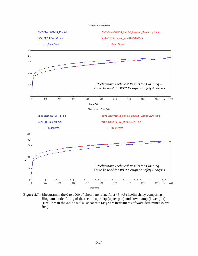
5.24
Figure 5.7. Rheogram in the 0 to 1000 s-1
shear rate range for a 43 wt% kaolin slurry comparing
Bingham model fitting of the second up ramp (upper plot) and down ramp (lower plot).
(Red lines in the 200 to 800 s-1
shear rate range are instrument software determined curve
fits.)
0
50
100
150
200
Pa
0 100 200 300 400 500 600 700 800 900 1,0001/s
Shear Rate .
Shear Stress vs Shear Rate
23-03-Stock-081414_Run 2-2
CC27-SN13634; d=0 mm
Shear Stress
23-03-Stock-081414_Run 2-2_Bingham_Second Up Ramp
tau0 = 110.85 Pa; eta_inf = 0.062784 Pa·s
Shear Stress
0
50
100
150
200
Pa
0 100 200 300 400 500 600 700 800 900 1,0001/s
Shear Rate .
Shear Stress vs Shear Rate
23-03-Stock-081414_Run 2-2
CC27-SN13634; d=0 mm
Shear Stress
23-03-Stock-081414_Run 2-2_Bingham_Second Down Ramp
tau0 = 129.04 Pa; eta_inf = 0.048479 Pa·s
Shear Stress
Preliminary Technical Results for Planning –
Not to be used for WTP Design or Safety Analyses
Preliminary Technical Results for Planning –
Not to be used for WTP Design or Safety Analyses
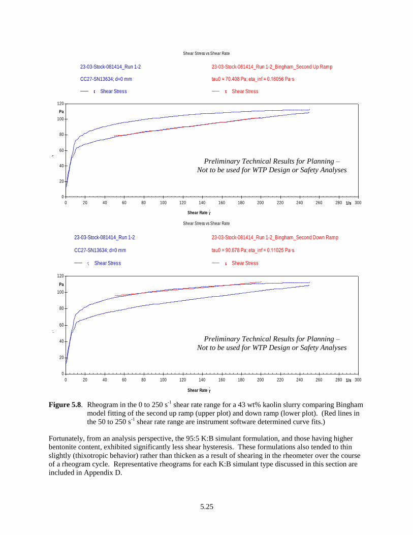
5.25
Figure 5.8. Rheogram in the 0 to 250 s-1
shear rate range for a 43 wt% kaolin slurry comparing Bingham
model fitting of the second up ramp (upper plot) and down ramp (lower plot). (Red lines in
the 50 to 250 s-1
shear rate range are instrument software determined curve fits.)
Fortunately, from an analysis perspective, the 95:5 K:B simulant formulation, and those having higher
bentonite content, exhibited significantly less shear hysteresis. These formulations also tended to thin
slightly (thixotropic behavior) rather than thicken as a result of shearing in the rheometer over the course
of a rheogram cycle. Representative rheograms for each K:B simulant type discussed in this section are
included in Appendix D.
0
20
40
60
80
100
120
Pa
0 20 40 60 80 100 120 140 160 180 200 220 240 260 280 3001/s
Shear Rate .
Shear Stress vs Shear Rate
23-03-Stock-081414_Run 1-2
CC27-SN13634; d=0 mm
Shear Stress
23-03-Stock-081414_Run 1-2_Bingham_Second Up Ramp
tau0 = 70.408 Pa; eta_inf = 0.16056 Pa·s
Shear Stress
0
20
40
60
80
100
120
Pa
0 20 40 60 80 100 120 140 160 180 200 220 240 260 280 3001/s
Shear Rate .
Shear Stress vs Shear Rate
23-03-Stock-081414_Run 1-2
CC27-SN13634; d=0 mm
Shear Stress
23-03-Stock-081414_Run 1-2_Bingham_Second Down Ramp
tau0 = 90.678 Pa; eta_inf = 0.11025 Pa·s
Shear Stress
Preliminary Technical Results for Planning –
Not to be used for WTP Design or Safety Analyses
Preliminary Technical Results for Planning –
Not to be used for WTP Design or Safety Analyses

5.26
Although Bingham yield stress and consistency are typically treated independently for defining simulant
property targets, it is the combination of the two parameters that may be most pertinent for defining the
overall characteristics of merit for mixing and/or gas release studies. Using the Bingham plastic model,
yield stress and consistency together define the shear stress (Eq. 5.13) and the effective (or apparent)
viscosity (Eq. 5.14) as they vary with shear rate. Using the method outlined in Section 5.5.2.2 and
the exponential curve fits for τ0 and μ∞ as a function of weight percent solids (see Figure 5.5 and
Appendix D), the consistency at constant yield stresses of 30 Pa and 15 Pa were determined for each K:B
simulant formulation. Subsequently, the apparent viscosity at τ0 = 30 Pa or 15 Pa as a function of applied
shear rate was estimated using Eq. 5.14. Figure 5.9 shows the calculated μapp values in the shear rate
range of 100 to 10,000 s-1
using up-ramp (upper plot) and down-ramp (lower plot) Bingham parameter
fits. Each plot shows decreasing effective viscosity with increasing shear rate and a transition from yield-
stress dominated effect at lower shear rate to consistency-governed μapp at higher shear rate. At 100 s-1
shear rate, for example, the apparent viscosity is given approximately by the ratio τ0/ (300 cP) for all
simulant types shown in Figure 5.9. At ≥10,000 s-1
shear rate, μapp asymptotically approaches μ∞. From a
waste (simulant) transport perspective, in which shear rate may vary cyclically (e.g., PJM operations1)
and by location in a process vessel, it is noteworthy in Figure 5.9 that μapp decreases by about an order of
magnitude from a nearly constant value of ~300 cP at relatively low shear rate for all the simulant types
to 16 cP ≤ μapp ≤ 41 cP at 10,000 s-1
. The latter is comparable to the range of Bingham consistencies for
τ0 = 30 Pa (~10 cP < μ∞ < 40 cP).
Figure 5.9 shows that the apparent viscosity at each shear rate for K:B in water formulations follows the
trend: 100 percent kaolin < 98:2 K:B < 95:5 K:B < 90:10 K:B < 80:20 K:B. This ordering is opposite
that for the yield stress-to-consistency ratio shown in the lower plot of Figure 5.6, or alternatively, is the
same as that for the inverted ratio μ∞/τ0. The latter reflects decreasing Bingham consistency at constant
yield stress (e.g., 30 Pa) with increasing kaolin fraction. The behavior of 80:20 K:B adjusted to pH 4 to 5
in Figure 5.9 is more similar to 100 percent kaolin and 98:2 K:B than it is to 80:20 K:B in water, which is
again consistent with yield stress-to-consistency ratio data in Figure 5.6. Likewise, the 95:5 K:B in
10 wt% NaCl recipe had even higher τ0/μ∞ than 100 percent kaolin and would have lower apparent
viscosity as a function of shear rate than kaolin if it were plotted in Figure 5.9. The shear rate dependence
of apparent viscosity for the 90:10 M30:B, pH 4 to 5 formulation that was developed as a Hanford tank
waste simulant for the study of RT instability gas releases (Rassat et al. 2014) is shown in Figure 5.9
(lower plot) for comparison.2 The results are nearly identical to those for the 80:20 K:B in water recipe.
The progression of decreasing μapp with decreasing bentonite content for K:B/water recipes holds for both
the down-ramp and up-ramp analyses depicted in Figure 5.9. However, the spread of the up-ramp data is
slightly less than that for the down-ramp results. For example, the consistency values (μ∞ ≈ μapp at
10,000 s-1
) at τ0 = 30 Pa using down-ramp data range from 16 to 39 cP for 100 percent kaolin and 80:20
K:B in water, respectively, and the range is 22 to 37 cP for the same materials in the up-ramp analysis.
The relative apparent viscosity, up ramp/down ramp, derived from the data in Figure 5.9 is shown in
Figure 5.10 for the various K:B formulations. It shows maximum variability at high shear rate,
approaching the up- to down-ramp ratio of μ∞. The greatest ratio shown in Figure 5.10 (1.35 at
10,000 s-1
) is for 100 percent kaolin, which demonstrated the greatest hysteresis in rheograms obtained for
the various K:B formulations. The positive ratio reflects the impact of up- and down-ramp fitting on
Bingham consistency. As noted in the discussion around Figure 5.7 and Figure 5.8, the observed
1 A For-Information-Only numerical simulation of a pulse jet operating at a drive velocity of 12 m/s in a proposed
WTP vessel design using simulated waste of 1.2 g/mL density and 30 cP (Newtonian) viscosity indicated a peak
wall (vessel bottom head) shear rate of ~40,000 s-1
. (Email communication from Kurt Recknagle on June 1, 2015.) 2 The analysis used exponential correlations for Bingham yield stress and consistency as a function of solids content
that are given in Section 7.1.3 and shown in Figure 7.5 of Rassat et al. (2014). Only standard down-ramp rheology
data are presented there and used here.
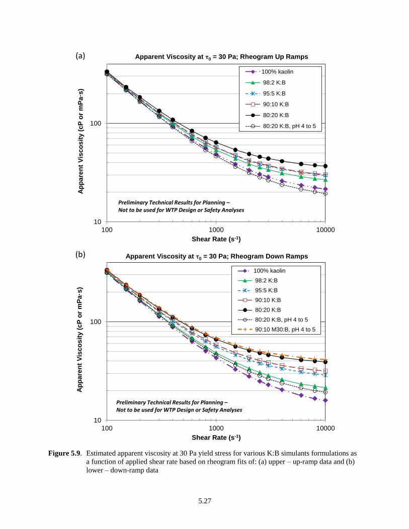
5.27
Figure 5.9. Estimated apparent viscosity at 30 Pa yield stress for various K:B simulants formulations as
a function of applied shear rate based on rheogram fits of: (a) upper – up-ramp data and (b)
lower – down-ramp data
10
100
100 1000 10000
Ap
pa
ren
t V
isc
os
ity (
cP
or
mP
a·s
)
Shear Rate (s-1)
Apparent Viscosity at τ0 = 30 Pa; Rheogram Up Ramps
100% kaolin
98:2 K:B
95:5 K:B
90:10 K:B
80:20 K:B
80:20 K:B, pH 4 to 5
Preliminary Technical Results for Planning –Not to be used for WTP Design or Safety Analyses
(a)
10
100
100 1000 10000
Ap
pa
ren
t V
isc
os
ity (
cP
or
mP
a·s
)
Shear Rate (s-1)
Apparent Viscosity at τ0 = 30 Pa; Rheogram Down Ramps
100% kaolin
98:2 K:B
95:5 K:B
90:10 K:B
80:20 K:B
80:20 K:B, pH 4 to 5
90:10 M30:B, pH 4 to 5
Preliminary Technical Results for Planning –Not to be used for WTP Design or Safety Analyses
(b)

5.28
thickening (rheopectic) behavior of kaolin results in relatively higher consistency and lower yield stress in
fitting the rheogram up ramp compared to the down ramp. The lowest apparent viscosity ratio in
Figure 5.10 is 0.94 for 80:20 K:B in water, and the result being slightly <1 is attributed to the modest
thinning (thixotropic) behavior noted in discussion above.
Figure 5.10. Ratio of rheogram up-ramp- to down-ramp-based estimates of apparent viscosity at 30 Pa
yield stress for various K:B simulants formulations as a function of applied shear rate
Results that trend similar to those shown in Figure 5.9 and Figure 5.10 are obtained if the analysis is
repeated for a Bingham yield stress of 15 Pa (or other τ0 < 30 Pa). If, however, the analysis is repeated
using constant shear strength instead of yield stress as a basis,1 the results differ measurably though the
difference is affected to some degree by the uncertainty in the correlations used to make this comparison.
Figure 5.11 shows such an analysis for τS = 15 Pa using only the rheogram down-ramp fits. Compared to
Figure 5.9 (lower plot), the most obvious differences exhibited in Figure 5.11 are: a) higher, rather than
lower, apparent viscosity for formulations having greater kaolin content and b) substantial spread in the
range of μapp values at lower shear rate. The latter is due primarily to not fixing the yield stress, which
substantially governs the apparent viscosity at low shear rate. Figure 5.11 shows that 100 percent kaolin
has an estimated μapp of ~620 Pa at 100 s-1
, which is ~5 times higher than for 80:20 K:B in water. This is
consistent with the upper plot of Figure 5.6 which shows a similar relationship in the ratio of yield
stresses at 15 Pa shear strength (plotted there inversely as τ0/τS). Although not as readily discerned, data
in Figure 5.6 shows that μ∞ is relatively constant, compared to τ0, for the various K:B in water
formulations at τS = 15 Pa. This is reflected in μapp at 10,000 s-1
, or similarly μ∞, differing by less than a
factor of 1.6 for these recipes (Figure 5.11). However, it can be shown using the data in Figure 5.6 that
1 The methodology is analogous to that described in Section 5.5.2.2 and used for the constant yield stress analysis
except that exponential correlations for shear strength vs. weight percent solids are inverted to determine the solids
content at the target τS (e.g., 15 Pa). Subsequently, xS is used to calculate τ0 and μ∞, and in turn, μapp.
0.9
1
1.1
1.2
1.3
1.4
10 100 1000 10000
Ap
pare
nt
Vis
co
sit
y R
ati
o (
Up
/Do
wn
Ram
ps)
Shear Rate (s-1)
Apparent Viscosity Ratio for τ0 = 30 Pa
100% kaolin
98:2 K:B
95:5 K:B
90:10 K:B
80:20 K:B
80:20 K:B, pH 4 to 5
Preliminary Technical Results for Planning –Not to be used for WTP Design or Safety Analyses
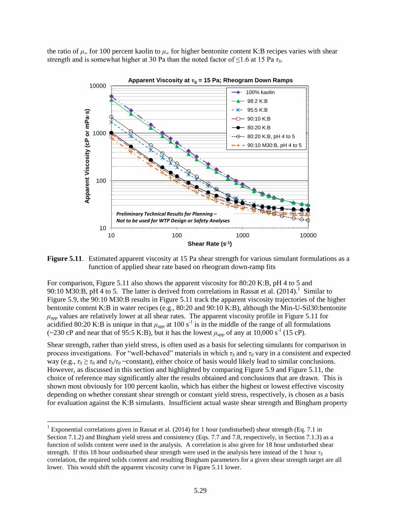
5.29
the ratio of μ∞ for 100 percent kaolin to μ∞ for higher bentonite content K:B recipes varies with shear
strength and is somewhat higher at 30 Pa than the noted factor of ≤1.6 at 15 Pa τS.
Figure 5.11. Estimated apparent viscosity at 15 Pa shear strength for various simulant formulations as a
function of applied shear rate based on rheogram down-ramp fits
For comparison, Figure 5.11 also shows the apparent viscosity for 80:20 K:B, pH 4 to 5 and
90:10 M30:B, pH 4 to 5. The latter is derived from correlations in Rassat et al. (2014).1 Similar to
Figure 5.9, the 90:10 M30:B results in Figure 5.11 track the apparent viscosity trajectories of the higher
bentonite content K:B in water recipes (e.g., 80:20 and 90:10 K:B), although the Min-U-Sil30:bentonite
μapp values are relatively lower at all shear rates. The apparent viscosity profile in Figure 5.11 for
acidified 80:20 K:B is unique in that μapp at 100 s-1
is in the middle of the range of all formulations
(~230 cP and near that of 95:5 K:B), but it has the lowest μapp of any at 10,000 s-1
(15 cP).
Shear strength, rather than yield stress, is often used as a basis for selecting simulants for comparison in
process investigations. For “well-behaved” materials in which τS and τ0 vary in a consistent and expected
way (e.g., τS ≥ τ0 and τS/τ0 ~constant), either choice of basis would likely lead to similar conclusions.
However, as discussed in this section and highlighted by comparing Figure 5.9 and Figure 5.11, the
choice of reference may significantly alter the results obtained and conclusions that are drawn. This is
shown most obviously for 100 percent kaolin, which has either the highest or lowest effective viscosity
depending on whether constant shear strength or constant yield stress, respectively, is chosen as a basis
for evaluation against the K:B simulants. Insufficient actual waste shear strength and Bingham property
1 Exponential correlations given in Rassat et al. (2014) for 1 hour (undisturbed) shear strength (Eq. 7.1 in
Section 7.1.2) and Bingham yield stress and consistency (Eqs. 7.7 and 7.8, respectively, in Section 7.1.3) as a
function of solids content were used in the analysis. A correlation is also given for 18 hour undisturbed shear
strength. If this 18 hour undisturbed shear strength were used in the analysis here instead of the 1 hour τS
correlation, the required solids content and resulting Bingham parameters for a given shear strength target are all
lower. This would shift the apparent viscosity curve in Figure 5.11 lower.
10
100
1000
10000
10 100 1000 10000
Ap
pa
ren
t V
isc
os
ity (
cP
or
mP
a·s
)
Shear Rate (s-1)
Apparent Viscosity at τS = 15 Pa; Rheogram Down Ramps
100% kaolin
98:2 K:B
95:5 K:B
90:10 K:B
80:20 K:B
80:20 K:B, pH 4 to 5
90:10 M30:B, pH 4 to 5
Preliminary Technical Results for Planning –Not to be used for WTP Design or Safety Analyses

5.30
data (e.g., as a function of solids content and strength) was found to interpolate or extrapolate to a
constant shear strength (or yield stress) for comparison to the simulant analysis completed in this section.
5.5.3.3 Gas Generation Rate in Kaolin:Bentonite Simulants
Gas generation rate may be a factor in the characteristics of gas release from simulants. Therefore, to put
different simulant formulations on the same footing in this regard so that other factors may be investigated,
information is needed on variation in gas generation rate with simulant type and how to control or adjust it.
Controlling the rate, or understanding it at least, is also important for reasons of experimental practicality.
For example, in experiments where H2O2 is used to generate oxygen bubbles and all of it is added to the
batch ex situ before the start of a test, rather than continuously during the test, it is preferable that the initial
gas generation rate be relatively low so significant quantities of gas are not produced (and retained) while
the test vessel is loaded. This would be a consideration for emplacing a gas-generating dead zone in
predominantly non-gas-generating simulant (see Section 6.3.3), the process of which may be longer than a
typical vessel filling operation. Rassat et al. (2014) considered this in the development of a 90:10 M30:B
simulant for RT instability gas release tests. They demonstrated in FIO tests that the gas generation rate
increased with the amount (concentration) of H2O2 added, as expected, and that acidification of the
simulant to between pH 4 and 5 reduced the initial rate of O2 production by more than a factor of 5.1 The
latter is due, at least in part, to known stabilization of H2O2 (solution) at pH < 5.
Five gas generation rate tests were completed in 500 mL and 1 L graduated cylinders using 98:2, 95:5,
90:10, and 80:20 K:B in water simulants and a sample of acidified 80:20 K:B. The pre-H2O2 slurry
samples for each were taken from KitchenAid batches that had been prepared for additional
characterization (e.g., rheology discussed in the previous section). Because the batches were
dual-purpose and were not prepared after correlations of rheological properties had been developed, they
did not have consistent physical properties (e.g., yield stress). However, the target initial concentration of
H2O2 in the slurry was held constant at 0.20 wt%. Table 5.2 summarizes simulant recipe and property
information for the samples used in the gas generation rate tests. Properties shown include the theoretical
gas-free slurry density (see Section 5.5.2.2) and (gas-free) rheological properties estimated from
exponential correlations discussed in Section 5.5.3.2 and tabulated in Appendix D using the post-
H2O2-addition solids content shown in Table 5.2.
Figure 5.12 shows the gas generation rates of the samples as measured over ~2 days or more (upper) and
the “initial” rate in the first 5 hours (lower). The amount of gas generated is quantified in terms of the
retained gas volume fraction, α, which is the ratio of retained gas volume to total gaseous slurry volume
(measured directly from the graduated cylinder). The gas volume as a function of time was determined as
the difference of the measured total volume and the gas-free initial slurry volume, which was calculated
as the product of the theoretical gas-free slurry density and the mass of slurry added to the cylinder.
Elapsed time (ET) 0 is defined as the time that the graduated cylinder was filled (to ~50 percent volume)
and a first level measurement was made, which was typically ~10 minutes or less after the start of the
addition of H2O2 solution to and hand-mixing of the slurry for ~1 to 3 minutes. Non-zero gas fractions at
ET 0 in Figure 5.12 reflect initially retained gas in the slurry resulting from generation and/or entrainment
before and during the fill process and uncertainty in the calculation of the gas-free initial volume. Strictly
speaking, the figure shows the rate of gas retention and not gas generation. They are essentially equal in
the absence of release events and neglecting the small amount of gas generated from the near-surface
layer. There was no visual evidence of substantive gas releases during the period of data acquisition;
however, not all tests were monitored continuously (i.e., no video in several tests). The smooth trajectory
of the data sets in the first ~5 hours, in which the tests were monitored more frequently, further suggests
that no episodic releases occurred and that nearly 100 percent of the generated gas was retained.
1 See Figure 5.1 in Section 5.1.2 of Rassat et al. (2014).

5.31
Although their rheological properties differ significantly (Table 5.2), the 80:20 K:B samples were
identical in composition except for acidification of the “80:20 K:B, pH 4 to 5” formulation. Therefore,
differences in gas generation rate shown in Figure 5.12 are attributed to pH effects. At ~1.2 hours, the
retained gas fraction in the unmodified slurry (pH 6.6 to 6.9 typical, pre-H2O2) was twice that of the slurry
adjusted to pH 4.3 to 4.6 (e.g., α = 0.20 vs. 0.10). In absolute terms, such as the volume of gas generated
for the nominally equal initial volumes of slurry, the generation rate of the higher-pH simulant was about
4-times faster in this time period on average.1 Figure 5.12 also shows that less total gas was generated in
the low-pH sample, as determined by the maximum, and apparently steady, α values at long time. Based
on the amount of H2O2 added, the theoretical maximum gas fraction (assuming 100 percent retention) for
all the tests shown is in the range 0.46 to 0.49. Therefore, it appears that the yield of gas in the 80:20 K:B
sample that was not acidified was near 100 percent.
Table 5.2. Properties of kaolin:bentonite (K:B) simulants used in gas generation rate tests
Simulant
Type
Source
Batch
I.D.
Weight Fractions in Slurry
(wt%)
H2O2
Conc.(b)
(M)
Gas-Free
ρS(c)
(g/mL) ~pH(d)
Est. Rheological
Properties(a)
Total
Solids
(xS)
K/B
Solids H2O2
τS
(Pa)
τ0
(Pa)
μ∞
(cP)
98:2 K:B 102014D 41.3 40.5/0.8 0.20 0.100 1.344 5.2 14 48 25
95:5 K:B 102014B 40.4 38.4/2.0 0.20 0.098 1.333 6.1 14 15 20
90:10 K:B 102014A 37.6 33.8/3.8 0.20 0.094 1.302 6.7 20 12 21
80:20 K:B 090914A 29.1 23.3/5.8 0.20 0.083 1.218 6.6-6.9 6 4 16
80:20 K:B,
pH 4 to 5 090914B 29.1 23.3/5.8 0.20 0.083 1.218 4.3-4.5 26 36 19
Preliminary Technical Results for Planning – Not to be used for WTP Design or Safety Analyses
(a) Shear strength and Bingham yield stress and consistency (down-ramp fits) were estimated for the tabulated
post-H2O2 addition total solids content (xS) using the exponential correlations shown graphically in Figure 5.5
of Section 5.5.3.2 and summarized numerically in Appendix D.
(b) Calculated molar (M, mol/L) concentration of H2O2 in the liquid phase of the slurry.
(c) The theoretical gas-free slurry density is calculated using Eq. 5.12 in Section 5.5.2.2.
(d) The reported approximate pH values are for samples of the same formulation but without H2O2 added, and in
some cases the samples were at different solids concentrations than shown tabulated here. In addition, the
time between batch or sample preparation and the pH measurement differed for some samples. However, the
pH of acidified slurry (and others that are not pH adjusted) tends to be stabile after equilibrating a day or
longer. The reported pH for “80:20 K:B, pH 4 to 5” was taken more than 24 hours after preparation.
Similarly, Figure 5.12 shows that the gas yield was about 100 percent for 90:10 K:B, but that it decreased
progressively with decreasing bentonite fraction in the 95:5 K:B and 98:2 K:B simulants. The gas
generation rates followed the same trend for these 3 samples, i.e., increasing rate (and total production)
with increasing bentonite content. The generation rate in the 90:10 K:B slurry was higher even though
the molar concentration of H2O2 in the liquid phase shown in Table 5.2 was about 4 to 6 percent less than
1 In this case, the difference in generation rates is also approximated by the ratio of the change in α in the time
period, noting that α at ET 0 differed for the two tests. More generally: in absolute terms, the volume of gas
generated in a time period is referenced to the initial volume (or mass) of gas-free slurry, whereas in the calculation
of α, the reference volume in the denominator also includes the volume of gas generated (i.e., α = volume of gas
generated /[initial volume of gas-free slurry + volume of gas generated]). The absolute and relative measures differ
exactly by a factor of 2 when the volume of gas generated is equal to the initial slurry volume (100 percent change),
for which α = 0.5 (50 vol%; if all generated gas is retained in the slurry). On the other hand, the ratio of absolute
and relative measures approaches 1 for α near 0.
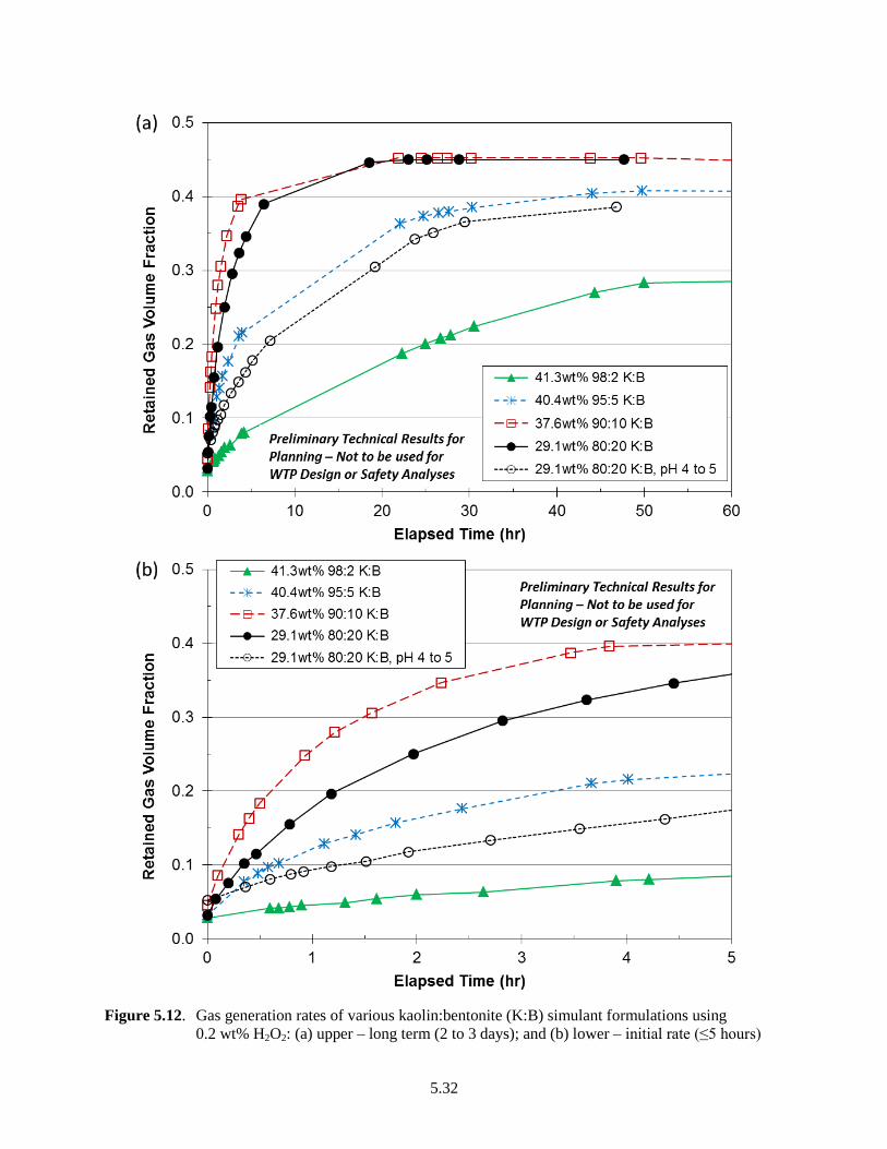
5.32
Figure 5.12. Gas generation rates of various kaolin:bentonite (K:B) simulant formulations using
0.2 wt% H2O2: (a) upper – long term (2 to 3 days); and (b) lower – initial rate (≤5 hours)

5.33
the 95:5 K:B and 98:2 K:B slurries, respectively.1 The reduced generation rate with increasing kaolin
fraction in this series of samples may correlate with decreasing pH. The pH values measured on pre-H2O2
samples of the same formulation (if not the same batch) were 6.7, 6.1, and 5.2 for 90:10 K:B, 95:5 K:B,
and 98:2 K:B, respectively. Additional data taken on samples after H2O2 addition and reaction showed
that the pH was 0.2 to 0.8 units lower. This may be due in part to the slight acidity of the H2O2 solution
(e.g., pH ~5). It should also be noted that the pH of 100 percent kaolin slurry is typically ~4.5.
Therefore, the higher pH of K:B simulants are due to the alkalinity of bentonite.
The differences in generation rate of 90:10 K:B and 80:20 K:B in water simulants shown in Figure 5.12
do not appear to be due to pH effects (i.e., both were in the pH 6.6 to 6.9 range). The higher generation
rate in 90:10 K:B may be associated with the molar concentration of H2O2, which was 13 percent higher,
although it had less bentonite than the 80:20 K:B sample (3.8 wt% compared to 5.8 wt%). However, it
cannot be determined conclusively from all the data presented whether the bentonite content was a factor
in gas generation rate in addition to H2O2 concentration and (its effect on) pH. This might be answered
by an experiment that is the converse of acidifying 80:20 K:B to slow it down, e.g., increasing the pH of
initially low-pH high-kaolin content slurries. Such an experiment was not attempted in these preliminary
gas generation rate studies. Reaction rates and gas yields are anticipated to increase at higher pH even if
the bentonite fraction is less than 10 wt%.
5.5.3.4 Settling in Low Yield Stress Non-Newtonian Kaolin:Bentonite Simulants
Stability against significant settling of solids and formation of free-liquid layers is another consideration
for non-Newtonian simulants, especially for materials at the lower bound of Bingham yield stress (e.g., τ0
≤6 Pa). Gravity settling was briefly investigated for the weakest of the 98:2 K:B, 95:5 K:B, and
90:10 K:B recipes that had nominally been prepared for rheological characterization. Mixed samples
were added to 500 mL graduated cylinders to near capacity (492 to 498 mL), corresponding to a height 2
of ~30 cm, and allowed to stand undisturbed on a lab bench. The surface level, i.e., total volume, and
settled-solids/supernatant liquid interface volume were tracked for ~3 weeks. It was initially anticipated
that the parallel tests would be run for only a day or two, so steps to mitigate evaporative losses were
minimal (e.g., only loosely covered). The total volume decreased by approximately 3 percent over the
course of the study due to evaporation.3 To correct for evaporation effects, the initial total volume was
used as the reference for determining the volume fractions of supernatant liquid and the settled solids
layer as a function of time. It was further assumed that the small change in height and liquid head had
negligible impact on the degree of settling.
Figure 5.13 and Table 5.3 show that the volume fraction of supernatant liquid increased both with time
and increasing fraction of kaolin. After a week to 10 days, the separated liquid was ~2 to 3 vol% for
90:10 K:B, 4 to 5 vol% for 95:5 K:B, and ~5 to 6 vol% for 98:2 K:B. As noted in Table 5.3, the
measured shear strength and yield stress were 7 Pa and 20 Pa, respectively, for the 98:2 K:B batch,
whereas both strength measurements were ≤~2 Pa for the 95:5 K:B and 90:10 K:B. Therefore, the
relatively greater settling of the 98:2 K:B simulant is attributed to its high kaolin fraction and not
differences in strength. Note also that the total solids content of the 95:5 K:B (33 wt% solids) and
90:10 K:B (31 wt% solids) recipes were lower than for the 98:2 K:B (38 wt% solids). The reduced
1 Differences in H2O2 molar concentration in the liquid phase for constant weight percent concentration (e.g.,
0.20 wt% of the slurry) arise from different total solids fractions in and corresponding densities of the slurries. 2 The reported height is from post-test measurements of representative 500-mL graduated cylinders found in the lab:
one was 27 cm and another brand was 30 cm. 3 The evaporative loss is based on difference of the initial and final surface level measurements and confirmed by
mass loss estimates, where the initial mass was calculated from initial volume and theoretical density and the final
mass was measured.

5.34
settling of the former two at lower-solids content and strength is likely attributed to differences in
morphology of the bentonite and kaolin particles and the associated cohesive nature of bentonite.
Figure 5.13. Settling of various “weak” non-Newtonian kaolin:bentonite (K:B) simulant formulations
Kaolin and 80:20 K:B simulants were developed for use in testing prospective transuranic (TRU) waste
processing systems (Rassat et al. 2003). Using actual waste sample measurements as reference,
100 percent kaolin recipes were selected to have characteristic gravity settling behavior, and 80:20 K:B
simulant was chosen for representative centrifugal dewatering and transport properties (e.g., rheology).
Select gravity settling results from the earlier study (labeled with the report number PNNL-14333 for
Rassat et al. [2003]) are shown in Table 5.3 and Figure 5.13 for comparison to the presently evaluated
K:B formulations. 40 wt% kaolin exhibited equal or greater settling than 38 wt% 98:2 K:B in both the
reported “scoping” and “validation” tests.1 Figure 5.13 shows that greater settling, up to ~14 vol%
supernatant liquid in ~7.5 days, was observed in the scoping test; other than the noted use of different
bags of clay, the difference in these test results is not discussed in the report. Regardless, the trend of
1 Both centrifugal dewatering and gravity settling tests reported in Rassat et al. (2003) used 50-mL graduated plastic
centrifuge tubes, which typically are less than half the height of a filled 500-mL graduated cylinder (e.g., <12 cm
from bottom to rim for Corning® 50-mL cone bottom centrifuge tubes). It is reported that ~35 mL and ~50 mL of
slurry were used in “scoping” and “validation” tests, respectively. Different bags and lot numbers of bentonite were
used in the two test types; it was postulated, but could not be confirmed, that the two bags of kaolin came from the
same lot. The bentonite and kaolin were the same grades and came from the same suppliers as those of the present
study.
0
2
4
6
8
10
12
14
0 5 10 15 20 25
Su
pern
ata
nt
Liq
uid
Vo
lum
e F
rac
tio
n (
vo
l%)
Elapsed Time (d)
38.0 wt% 98:2 K:B
33.0wt% 95:5 K:B
31.0wt% 90:10 K:B
21wt% 80:20 K:B (PNNL-14333)
40wt% kaolin (PNNL-14333 Validation)
40wt% kaolin (PNNL-14333 Scoping)
Preliminary Technical Results for Planning –Not to be used for WTP Design or Safety Analyses
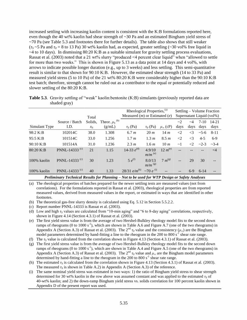
5.35
increased settling with increasing kaolin content is consistent with the K:B formulations reported here,
even though the 40 wt% kaolin had shear strength of ~30 Pa and an estimated Bingham yield stress of
~70 Pa (see Table 5.3 and footnotes there for further details). The table also shows that still weaker
(τS ~5 Pa and τ0 = 8 to 13 Pa) 30 wt% kaolin had, as expected, greater settling (~30 vol% free liquid in
~4 to 10 days). In dismissing 80:20 K:B as a suitable simulant for gravity settling process evaluations,
Rassat et al. (2003) noted that a 21 wt% slurry “produced <4 percent clear liquid” when “allowed to settle
for more than two weeks.” This is shown in Figure 5.13 as a data point at 14 days and 4 vol%, with
arrows to indicate possible longer duration (e.g., up to 3 weeks) and less settling. This semi-quantitative
result is similar to that shown for 90:10 K:B. However, the estimated shear strength (14 to 33 Pa) and
measured yield stress (5 to 10 Pa) of the 21 wt% 80:20 K:B were considerably higher than the 90:10 K:B
test batch; therefore, strength cannot be ruled out as a contributor to the equal or potentially reduced and
slower settling of the 80:20 K:B.
Table 5.3. Gravity settling of “weak” kaolin:bentonite (K:B) simulants (previously reported data are
shaded gray)
Simulant Type
Source / Batch
I.D.
Total
Solids,
xS
Theor. ρS (b)
(g/mL)
Rheological Properties,(a)
Measured (m) or Estimated (e)
Settling – Volume Fraction
Supernatant Liquid (vol%)
τS (Pa) τ0 (Pa) μ∞ (cP)
~2
days
~4
days
7-10
days
14-21
days
98:2 K:B 102014C 38.0 1.308 6.7 m 20 m 14 m <2 <3 ~5-6 8-11
95:5 K:B 101514C 33.0 1.256 1.7 m 1.3 m 8.5 m <2 <3 4-5 6-9
90:10 K:B 101514A 31.0 1.236 2.3 m 1.6 m 10 m ~1 <2 ~2-3 ~3-4
80:20 K:B PNNL-14333 (c)
21 1.15 14-33 e(d)
4.9/10
m/m (e)
12 m(e)
-- -- -- <4
100% kaolin PNNL-14333 (c)
30 1.23 5 e(f)
8.0/13
m/m (g)
7 m(g)
-- 29 30 --
100% kaolin PNNL-14333 (c)
40 1.33 28/31 e/m(h)
~70 e (i)
-- -- 6-9 6-14 --
Preliminary Technical Results for Planning – Not to be used for WTP Design or Safety Analyses
(a) The rheological properties of batches prepared for the newer settling tests are measured values (not from
correlations). For the formulations reported in Rassat et al. (2003), rheological properties are from reported
measured values, derived from measured values in the report, or estimated in ways that are identified in other
footnotes.
(b) The theoretical gas-free slurry density is calculated using Eq. 5.12 in Section 5.5.2.2.
(c) Report number PNNL-14333 is Rassat et al. (2003).
(d) Low and high τS values are calculated from “10-min aging” and “6 to 8-day aging” correlations, respectively,
shown in Figure 4.14 (Section 4.3.1) of Rassat et al. (2003).
(e) The first yield stress value is from the average of two Hershel-Bulkley rheology model fits to the second down
ramps of rheograms (0 to 1000 s-1
), which are shown in Table A.6 and Figure A.7 (one of the two rheograms) in
Appendix A (Section A.3) of Rassat et al. (2003). The 2nd
τ0 value and the consistency (μ∞) are the Bingham
model parameters determined by hand-fitting a line to the rheogram in the 200 to 800 s-1
shear rate range.
(f) The τS value is calculated from the correlation shown in Figure 4.13 (Section 4.3.1) of Rassat et al. (2003).
(g) The first yield stress value is from the average of two Hershel-Bulkley rheology model fits to the second down
ramps of rheograms (0 to 1000 s-1
), which are shown in Table A.4 and Figure A.5 (one of the two rheograms) in
Appendix A (Section A.3) of Rassat et al. (2003). The 2nd
τ0 value and μ∞ are the Bingham model parameters
determined by hand-fitting a line to the rheogram in the 200 to 800 s-1
shear rate range.
(h) The estimated τS is calculated from the correlation shown in Figure 4.13 (Section 4.3.1) of Rassat et al. (2003).
The measured τS is shown in Table A.2) in Appendix A (Section A.3) of the reference.
(i) The same nominal yield stress was estimated in two ways: 1) the ratio of Bingham yield stress to shear strength
determined for 30 wt% kaolin in the row above was assumed constant and was applied to the estimated τS of
40-wt% kaolin; and 2) the down-ramp Bingham yield stress vs. solids correlation for 100 percent kaolin shown in
Appendix D of the present report was used.

5.36
It should be noted that 80:20 K:B correlations given in Rassat et al. (2003) result in much higher
shear strength for a specified solids content than those discussed in Section 5.5.3.2 and tabulated in
Appendix D. For example, the correlations in Appendix D give τS and τ0 <1 Pa for 21 wt% 80:20 K:B.
However, as shown in Figure 5.4 (Section 5.5.3.1), the ‘Rassat et al. Corr.’ (reproduced in Burns et al.
2010 from Rassat et al. 2003) for 100 percent kaolin is very similar to the new correlation developed from
the Test FG 23-02 large-batch samples. All together, these data suggest that the characteristics of the
bentonite used 10+ years ago were somehow different, although variance in mixing methods, sample
aging, and other factors cannot be ruled out.

6.1
6.0 Experimental Investigations of Bubble Cascade, Buoyant Displacement, Dead Zone, and Induced Gas Releases from
Non-Newtonian Simulants and Settling Solids Layers
Scenarios leading to potentially large spontaneous BC and BD gas releases in WTP process vessels are a
focal point of this report and planned work. This section describes preliminary experimental
investigations of spontaneous and induced gas releases that were completed in 1 L graduated cylinders
and 10 and 23 in. diameter flat-bottom vessels. Additionally, the results of previous studies of and
available data for BC gas releases from relatively weak waste (simulants) are summarized in Section 6.1.
The general approach, methods, and systems used in the new experimental investigations are outlined in
Section 6.2. Non-Newtonian simulants of the types described in Section 5.5 were used in a dead zone
spontaneous gas release test and tests of gas release induced by a single air-sparger or a mechanical
agitator. The additional test-specific experimental equipment and techniques used in these
non-Newtonian simulant tests and the test results are discussed in Section 6.3. The results of
experimental studies of gas retention in and releases from settled layers formed in situ from relatively
low-solids slurries are covered in Section 6.4. Originally planned objectives and success criteria are
included in the relevant sections.
6.1 Spontaneous Bubble-Cascade Gas Releases
Bubbles of hydrogen-containing gas are known to be generated and retained by radioactive waste slurries,
and this retention of hydrogen gas is a pervasive safety hazard that must be managed at many facilities in
the DOE complex. Spontaneous and rapid releases of retained hydrogen bubbles and potential flammable
conditions are primary concerns for nuclear safety accident analysis. Previous studies have identified the
BC gas release mechanism as significant when vessels and tanks contain relatively weak slurries with
shear strengths between a few and a hundred pascals. Radioactive waste slurries with shear strengths in
this range are expected in process vessels at the WTP, in blended waste feed for the WTP that will be
staged in Hanford waste tanks or in a potential future waste blending facility, and in waste storage tanks
at the Savannah River Site.
The overall objective of this proposed study was to quantify the conditions at the onset of the BC gas
releases and to measure the fraction of the inventory released and the rate of release. The objective and
success criteria that were developed as part of the planning for this effort are given in the following
section.
6.1.1 Objective and Success Criteria
TP-WTPSP-1401 identifies the following test objective for the effort on BC gas releases:
Test Objective 11 - Bubble-Cascade Release: Measure the retained gas fraction in slurry simulants at
the onset of spontaneous BC gas releases in the absence of a (or with a thin) supernatant liquid layer
for a range of simulant waste physical properties (e.g., shear strength and Bingham yield stress) that
are representative of those anticipated for WTP waste streams. Assess the role of simulant selection,
vessel diameter, vessel geometry, and presence of a supernatant layer on the onset of BC releases.
1 Gauglitz PA. 2015. Test Plan for Hydrogen Gas Release from Vessels Technical Issue Support. TP-WTPSP-
140, Rev. 0, Pacific Northwest National Laboratory.

6.2
Achievement of this test objective was to be gaged by satisfaction of the success criteria. These criteria
are as follows:
Establish a level-volume correlation for each test vessel
Measure retained gas fraction as a function of time through the BC release
Measure the shear strength, Bingham yield stress and consistency for the non-Newtonian simulant
compositions used in gas release testing
Obtain BC results for two or more physical simulants that are targeted to demonstrate a range of gas
release behavior
Compare BC release behavior in nominally 23 in. and 43 in. diameter vessels and in 23 in. vessels
having flat- and semi-elliptical-bottoms to confirm that the BC gas fraction is effectively
characteristic of the material, not the vessel geometry
Confirm BC release behavior with a thick supernatant layer for one example when a BC occurs at a
gas fraction below neutral buoyancy in the supernatant.
6.1.2 Technical Approach
The planned approach for studying BC was to conduct baseline (no mixing) BC release tests with a single
gas-generating slurry layer (and, possibly, a relatively thin supernatant liquid layer to improve the
accuracy of level measurements and quantification of retained gas volumes). Test parameters that were
chosen to vary during testing were simulant type and strength (for a given vessel configuration and slurry
depth), vessel diameter and bottom type and slurry depth (for a single simulant), and supernatant layer
thickness (to establish that buoyant displacement was not a factor). Where practicable, test conditions
were to parallel those used in dead zone tests.
At the time the flammable-gas testing tasks were shut down, BC testing had not been initiated. As a
consequence, this section discusses only the background of BC studies (Section 6.1.3) and the available
historical BC data (Section 6.1.4).
6.1.3 Background
The retention and release of hydrogen gas from radioactive waste slurries in process vessels and tanks is a
safety hazard that must be managed at many facilities in the DOE complex. The key scenario for nuclear
safety accident analysis is a spontaneous and rapid release of retained hydrogen bubbles that creates
flammable conditions in a process tank or vessel. Estimating the gas release quantity and the duration of
the release are important for the accident analysis.
Previous studies have identified the BC gas release mechanism as a significant mechanism for large and
rapid releases when vessels and tanks containing relatively weak slurries with shear strengths between a
few and a hundred pascals release. This mechanism is known to be important for WTP (Sherwood 2008)
and waste storage in large underground tanks (Hester 2003). The BC mechanism was first observed by
Gauglitz et al. (1996) and results showed that the onset of a BC depended on the strength of the bubbly
material and the vessel diameter. The description “bubble cascade” was first used by Stewart et al.
(1996), which also discussed the importance of this mechanism to Hanford single-shell tanks.
Figure 6.1 depicts both a BC and a situation where a BC does not occur. A BC is initiated when a
retained bubble that was initially stagnant in a waste slurry with a yield stress begins to rise, and its
motion interacts with bubbles in its path, shears adjacent waste, and enables a second bubble to begin
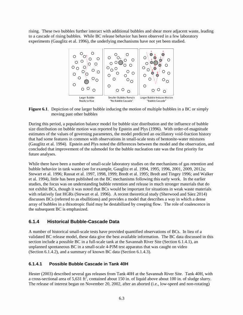
6.3
rising. These two bubbles further interact with additional bubbles and shear more adjacent waste, leading
to a cascade of rising bubbles. While BC release behavior has been observed in a few laboratory
experiments (Gauglitz et al. 1996), the underlying mechanisms have not yet been studied.
Figure 6.1. Depiction of one larger bubble inducing the motion of multiple bubbles in a BC or simply
moving past other bubbles
During this period, a population balance model for bubble size distribution and the influence of bubble
size distribution on bubble motion was reported by Epstein and Plys (1996). With order-of-magnitude
estimates of the values of governing parameters, the model predicted an oscillatory void-fraction history
that had some features in common with observations in small-scale tests of bentonite-water mixtures
(Gauglitz et al. 1994). Epstein and Plys noted the differences between the model and the observation, and
concluded that improvement of the submodel for the bubble nucleation rate was the first priority for
future analyses.
While there have been a number of small-scale laboratory studies on the mechanisms of gas retention and
bubble behavior in tank waste (see for example, Gauglitz et al. 1994, 1995, 1996, 2001, 2009, 2012a;
Stewart et al. 1996; Rassat et al. 1997, 1998, 1999; Bredt et al. 1995; Bredt and Tingey 1996; and Walker
et al. 1994), little has been published on the BC mechanisms following this early work. In the earlier
studies, the focus was on understanding bubble retention and release in much stronger materials that do
not exhibit BCs, though it was noted that BCs would be important for situations in weak waste materials
with relatively fast HGRs (Stewart et al. 1996). A recent theoretical study (Sherwood and Sáez 2014)
discusses BCs (referred to as ebullitions) and provides a model that describes a way in which a dense
array of bubbles in a thixotropic fluid may be destabilized by creeping flow. The role of coalescence in
the subsequent BC is emphasized.
6.1.4 Historical Bubble-Cascade Data
A number of historical small-scale tests have provided quantified observations of BCs. In lieu of a
validated BC release model, these data give the best available information. The BC data discussed in this
section include a possible BC in a full-scale tank at the Savannah River Site (Section 6.1.4.1), an
unplanned spontaneous BC in a small-scale 4-PJM test apparatus that was caught on video
(Section 6.1.4.2), and a summary of known BC data (Section 6.1.4.3).
6.1.4.1 Possible Bubble Cascade in Tank 40H
Hester (2003) described several gas releases from Tank 40H at the Savannah River Site. Tank 40H, with
a cross-sectional area of 5,631 ft2, contained about 150 in. of liquid above about 100 in. of sludge slurry.
The release of interest began on November 20, 2002, after an aborted (i.e., low-speed and non-rotating)
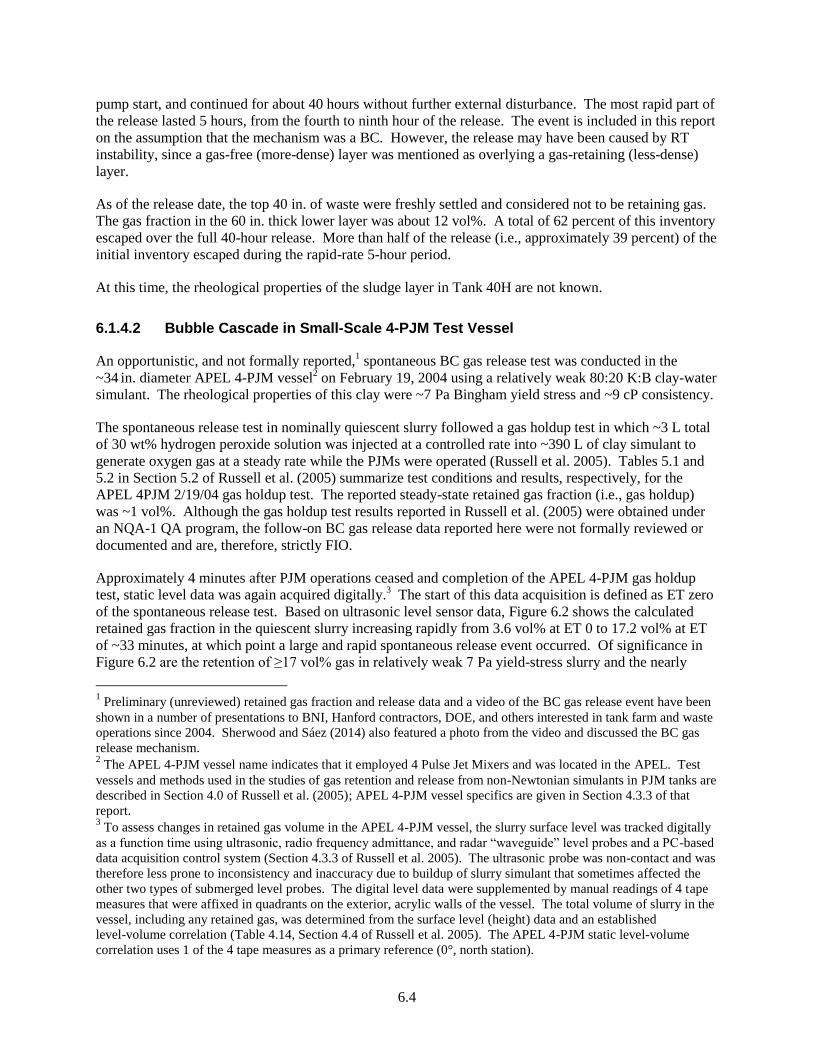
6.4
pump start, and continued for about 40 hours without further external disturbance. The most rapid part of
the release lasted 5 hours, from the fourth to ninth hour of the release. The event is included in this report
on the assumption that the mechanism was a BC. However, the release may have been caused by RT
instability, since a gas-free (more-dense) layer was mentioned as overlying a gas-retaining (less-dense)
layer.
As of the release date, the top 40 in. of waste were freshly settled and considered not to be retaining gas.
The gas fraction in the 60 in. thick lower layer was about 12 vol%. A total of 62 percent of this inventory
escaped over the full 40-hour release. More than half of the release (i.e., approximately 39 percent) of the
initial inventory escaped during the rapid-rate 5-hour period.
At this time, the rheological properties of the sludge layer in Tank 40H are not known.
6.1.4.2 Bubble Cascade in Small-Scale 4-PJM Test Vessel
An opportunistic, and not formally reported,1 spontaneous BC gas release test was conducted in the
~34 in. diameter APEL 4-PJM vessel
2 on February 19, 2004 using a relatively weak 80:20 K:B clay-water
simulant. The rheological properties of this clay were ~7 Pa Bingham yield stress and ~9 cP consistency.
The spontaneous release test in nominally quiescent slurry followed a gas holdup test in which ~3 L total
of 30 wt% hydrogen peroxide solution was injected at a controlled rate into ~390 L of clay simulant to
generate oxygen gas at a steady rate while the PJMs were operated (Russell et al. 2005). Tables 5.1 and
5.2 in Section 5.2 of Russell et al. (2005) summarize test conditions and results, respectively, for the
APEL 4PJM 2/19/04 gas holdup test. The reported steady-state retained gas fraction (i.e., gas holdup)
was ~1 vol%. Although the gas holdup test results reported in Russell et al. (2005) were obtained under
an NQA-1 QA program, the follow-on BC gas release data reported here were not formally reviewed or
documented and are, therefore, strictly FIO.
Approximately 4 minutes after PJM operations ceased and completion of the APEL 4-PJM gas holdup
test, static level data was again acquired digitally.3 The start of this data acquisition is defined as ET zero
of the spontaneous release test. Based on ultrasonic level sensor data, Figure 6.2 shows the calculated
retained gas fraction in the quiescent slurry increasing rapidly from 3.6 vol% at ET 0 to 17.2 vol% at ET
of ~33 minutes, at which point a large and rapid spontaneous release event occurred. Of significance in
Figure 6.2 are the retention of ≥17 vol% gas in relatively weak 7 Pa yield-stress slurry and the nearly
1 Preliminary (unreviewed) retained gas fraction and release data and a video of the BC gas release event have been
shown in a number of presentations to BNI, Hanford contractors, DOE, and others interested in tank farm and waste
operations since 2004. Sherwood and Sáez (2014) also featured a photo from the video and discussed the BC gas
release mechanism. 2 The APEL 4-PJM vessel name indicates that it employed 4 Pulse Jet Mixers and was located in the APEL. Test
vessels and methods used in the studies of gas retention and release from non-Newtonian simulants in PJM tanks are
described in Section 4.0 of Russell et al. (2005); APEL 4-PJM vessel specifics are given in Section 4.3.3 of that
report. 3 To assess changes in retained gas volume in the APEL 4-PJM vessel, the slurry surface level was tracked digitally
as a function time using ultrasonic, radio frequency admittance, and radar “waveguide” level probes and a PC-based
data acquisition control system (Section 4.3.3 of Russell et al. 2005). The ultrasonic probe was non-contact and was
therefore less prone to inconsistency and inaccuracy due to buildup of slurry simulant that sometimes affected the
other two types of submerged level probes. The digital level data were supplemented by manual readings of 4 tape
measures that were affixed in quadrants on the exterior, acrylic walls of the vessel. The total volume of slurry in the
vessel, including any retained gas, was determined from the surface level (height) data and an established
level-volume correlation (Table 4.14, Section 4.4 of Russell et al. 2005). The APEL 4-PJM static level-volume
correlation uses 1 of the 4 tape measures as a primary reference (0°, north station).
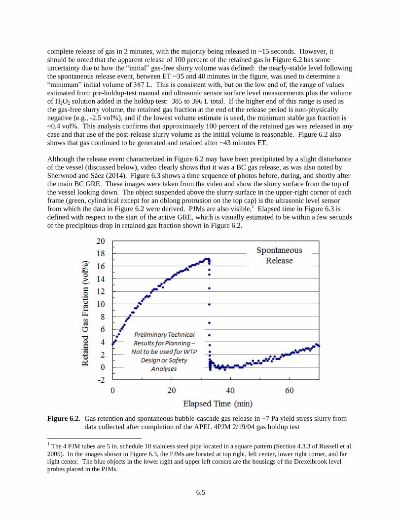
6.5
complete release of gas in 2 minutes, with the majority being released in ~15 seconds. However, it
should be noted that the apparent release of 100 percent of the retained gas in Figure 6.2 has some
uncertainty due to how the “initial” gas-free slurry volume was defined: the nearly-stable level following
the spontaneous release event, between ET ~35 and 40 minutes in the figure, was used to determine a
“minimum” initial volume of 387 L. This is consistent with, but on the low end of, the range of values
estimated from pre-holdup-test manual and ultrasonic sensor surface level measurements plus the volume
of H2O2 solution added in the holdup test: 385 to 396 L total. If the higher end of this range is used as
the gas-free slurry volume, the retained gas fraction at the end of the release period is non-physically
negative (e.g., -2.5 vol%), and if the lowest volume estimate is used, the minimum stable gas fraction is
~0.4 vol%. This analysis confirms that approximately 100 percent of the retained gas was released in any
case and that use of the post-release slurry volume as the initial volume is reasonable. Figure 6.2 also
shows that gas continued to be generated and retained after ~43 minutes ET.
Although the release event characterized in Figure 6.2 may have been precipitated by a slight disturbance
of the vessel (discussed below), video clearly shows that it was a BC gas release, as was also noted by
Sherwood and Sáez (2014). Figure 6.3 shows a time sequence of photos before, during, and shortly after
the main BC GRE. These images were taken from the video and show the slurry surface from the top of
the vessel looking down. The object suspended above the slurry surface in the upper-right corner of each
frame (green, cylindrical except for an oblong protrusion on the top cap) is the ultrasonic level sensor
from which the data in Figure 6.2 were derived. PJMs are also visible.1 Elapsed time in Figure 6.3 is
defined with respect to the start of the active GRE, which is visually estimated to be within a few seconds
of the precipitous drop in retained gas fraction shown in Figure 6.2.
Figure 6.2. Gas retention and spontaneous bubble-cascade gas release in ~7 Pa yield stress slurry from
data collected after completion of the APEL 4PJM 2/19/04 gas holdup test
1 The 4 PJM tubes are 5 in. schedule 10 stainless steel pipe located in a square pattern (Section 4.3.3 of Russell et al.
2005). In the images shown in Figure 6.3, the PJMs are located at top right, left center, lower right corner, and far
right center. The blue objects in the lower right and upper left corners are the housings of the Drexelbrook level
probes placed in the PJMs.
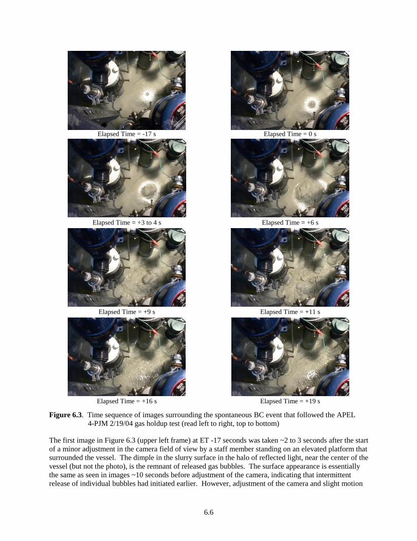
6.6
Elapsed Time = -17 s
Elapsed Time = 0 s
Elapsed Time = +3 to 4 s
Elapsed Time = +6 s
Elapsed Time = +9 s
Elapsed Time = +11 s
Elapsed Time = +16 s
Elapsed Time = +19 s
Figure 6.3. Time sequence of images surrounding the spontaneous BC event that followed the APEL
4-PJM 2/19/04 gas holdup test (read left to right, top to bottom)
The first image in Figure 6.3 (upper left frame) at ET -17 seconds was taken ~2 to 3 seconds after the start
of a minor adjustment in the camera field of view by a staff member standing on an elevated platform that
surrounded the vessel. The dimple in the slurry surface in the halo of reflected light, near the center of the
vessel (but not the photo), is the remnant of released gas bubbles. The surface appearance is essentially
the same as seen in images ~10 seconds before adjustment of the camera, indicating that intermittent
release of individual bubbles had initiated earlier. However, adjustment of the camera and slight motion
6.7
(jiggling) of the scaffolding structure, which ended at ET ~-2 seconds, may have triggered the larger
release event from the “ripe” gaseous slurry.
At ET 0 (upper-right frame in Figure 6.3), a ~3 to 5 cm diameter bubble is seen cresting at the slurry
surface. A bubble of this size is indicative of coalescence, because individual bubbles ~1.0 cm, and
possibly as small as 0.3 cm, should rise freely in ~7 Pa yield stress slurry (e.g., according to Eq. (4.2.9) in
Section 4.2.3 of Stewart et al. 1996).1 The photo at ET +3 to 4 seconds (2
nd row, left frame in Figure 6.3)
shows a cluster of large bubbles, now covering ≥ 10 cm diameter of the surface (by comparison to the
PJM tubes fabricated of 5 in. pipe). Images at +6, +9, and +11 seconds show the further cascade of
bubbles, as evidenced by the spread of bubbles across the surface and triggered by earlier motion that was
restricted to the center of the vessel at ET ≤ 0 seconds. By ET +16 seconds (lower left frame in
Figure 6.3), the majority of the gas release was visually complete, but slurry motion across the surface
continued. At ET +19 seconds (lower right frame) and later, surface motion stopped and bubbles in the
light froth layer popped sporadically. Coupled with the general decrease in level, surface motion and gas
release activity shown in Figure 6.3 likely contribute to the structure of the GRE depicted in Figure 6.2
(e.g., the negative peak in gas release near ET 33.1 minutes, -0.4 vol% gas fraction).
6.1.4.3 Summary of Bubble-Cascade Data
BCs have been observed fortuitously, as described in Section 6.1.4.2, and deliberately, in historical
experiments aimed at producing spontaneous releases that did not depend on the overall layer buoyancy
(Gauglitz et al. 1996; Rassat et al. 2014). The mechanism for these releases appeared to be BC.
The BC experiments used a cylindrical vessel containing a layer of simulant, consisting partly or
completely of clay, in which gas was generated by chemical reaction. The simulant layer had either no
supernatant liquid above it (Gauglitz et al. 1996) or a supernatant layer that was thin compared to the
solids layer (Rassat et al. 2014). The rheological properties of the simulant were measured from samples,
and the gas fraction history was calculated from measurements of the increase and decrease in the
elevation of the surface as gas was retained or released. Data were recorded during the experiments and
subsequently, based on videotaped observations. Table 6.1 lists the data obtained.
Figure 6.4 and Figure 6.5 show the gas fraction in the simulant at the time when the first release began
and the fraction of the inventory released (as calculated from the pre- and post-release surface levels).
Each curve or set of points is for a different vessel diameter and simulant. The plots relate the fraction
(on the y-axis) to the simulant shear strength, or to its yield stress (if shown in red) on the x-axis. A red
arrow, placed on the single point that was based on Bingham yield stress rather than shear strength,
indicates an approximate shear strength (in units of Pa) that is about two times the measured yield
strength, as suggested by Russell et al. (2005).
1 According to the relationship Db < τy/ρsgYG, where g is the acceleration of gravity, spherical bubbles of diameter Db
and smaller should be stable (remain motionless) in a quiescent non-Newtonian slurry having strength τy and
gas-free density ρs. Stewart et al. (1996) note that critical gravity-yield number, YG, is typically in the range 0.1 to
0.2 and is dependent on whether τy is defined as the Bingham yield stress or the shear strength from a vane
measurement (note that more recent evaluations use YG of ~ 0.06 [see discussion of Eq 4.2]). Using these values of
YG, and assuming a slurry density of 1,150 kg/m3 and a yield stress of 7 Pa, gives a stable bubble diameter ranging
from 0.3 to 0.6 cm. (The density is chosen to be less than the 1,180 kg/m3 given in Section 3.1 of Russell et al.
(2005) for a 27 wt% solids batch of slurry having 20 Pa yield stress. Without readily available information on the
solids content or slurry density used in the APEL 4-PJM 02/19/04 test, a lower density is assumed; for reference,
1,150 kg/m3 is the theoretical density of 21 wt% 80:20 K:B solids in water.)

6.8
Table 6.1. Data from bubble-cascade tests with simulants
Shear
Strength
(Pa)
Vessel
Diameter
(cm)
Gas
Fraction
Before
Release
Fraction
Of
Inventory
Released
Release As
Percent Of
Gas-Free
Slurry
Volume
Reference And
Simulant
1.3 2.54 0.01 n/a n/a Gauglitz et al. (1996);
bentonite 3.4 2.54 0.095 0.67 7
6.4 2.54 0.20 0.90 23
31 2.54 0.40 0.32 22
67 2.54 0.35 0.14 48
67 15.24 0.45 0.82 67
67 30.48 0.47 0.82 73
7(a)
86.36 0.17 0.98 20 Section 6.1.4.2;
80:20 kaolin:bentonite
16 58.42 0.30 0.99 43 Rassat et al. (2014);
90:10 Min-U-
Sil:bentonite 26 58.42 0.29 0.96 39
34 58.42 0.31 0.88 40
50 58.42 0.29 0.76 31
87 58.42 0.23 0.41 13
33 177.8 0.28 0.91 36
49 177.8 0.27 0.80 30
87 177.8 0.24 0.67 21
(a) This measurement value is the Bingham yield stress, not the shear strength. As
discussed in the text, the shear strength was probably about two times the yield stress.
Note: Preliminary Technical Results for Planning – Not to be used for WTP Design or
Safety Analyses
The widest range of simulant strengths that showed BCs, 1.3 to 67 Pa bentonite, was tested in a 2.54 cm
tube. Figure 6.4 shows that in this narrow container, the maximum onset gas fraction was about 0.4,
which was seen at a shear strength of 31 Pa (Gauglitz et al. 1996). The actual maximum may have been
at an non-measured shear strength between 31 and 67 Pa, but at 67 Pa the onset gas fraction was
definitely lower than at 31 Pa. The next higher shear strength that was tested in the 2.54 cm tube, 147 Pa,
showed a leveling-off of the gas fraction with no sudden release evident.
For the 67 Pa bentonite in wider containers, 15 and 30 cm, the gas fractions at the onset of BC were
higher—0.45 and 0.47—than at the 2.54 cm diameter. However, a similar range of shear strengths for a
different simulant in larger-diameter vessels (Rassat et al. 2014) gave lower gas fractions at onset—0.23
to 0.31. For this simulant and range of shear strengths, there was little difference between the onset
fractions for 58 and 178 cm diameters.
In the containers with 15 cm and 30 cm diameter, 200 Pa bentonite showed little evidence of BC releases.
Two tests with 200 Pa bentonite in a 15 cm container gave small releases, 10 percent or less of the
inventory. The same 200 Pa simulant in a 91 cm diameter container showed no sign of spontaneous
release. In this test, once the gas volume fraction reached about 49 percent, gas was released (perhaps
through small cracks) at the same rate at which it was generated, causing the gas fraction to remain
constant.

6.9
Figure 6.4. Gas fraction at onset of bubble-cascade release
Figure 6.5 shows the fraction of inventory released by the BCs in the historical tests. In general,
fractional releases 0.8 or higher were found for shear strengths of 50 Pa or less, but release fractions were
typically greater than 0.4. Some tendency for the fractional release to increase with vessel diameter can
be seen, but this trend is not consistent over all data sets; the nature of the simulant seems to have some
effect.
The release volume can also be expressed in terms of a fraction of the gas-free slurry volume, which may
be useful in some cases. As shown in Table 6.1, gas releases that were 20 to 40 percent of the gas-free
slurry volume were common for the larger vessel diameters (i.e., 58 to 178 cm).
Figure 6.5. Fraction of gas inventory released by bubble cascade

6.10
6.2 Experimental Methods and Systems for Gas Release Investigations
This section summarizes the experimental methods and systems used in the spontaneous and induced gas
release tests discussed in Section 6.3 and in the investigation of spontaneous gas releases from settling
solids layers (Section 6.4). Refer to Section 5.5.1 for a discussion of simulant materials and preparation
methods and Section 5.5.2 for information on methods used to characterize simulant physical and
chemical (e.g., pH) properties.
The spontaneous gas release tests are conceptually simple, as depicted schematically in Figure 6.6. Tests
are conducted in a cylindrical, open-topped, clear-plastic test vessel (or graduated cylinder) that is
(typically) placed on a scale to record the mass of simulant added and liquid lost due to evaporation, if
significant. For simplicity in this overview discussion, Figure 6.6 shows a generalized simulant
configuration consisting of a dead zone within a slurry layer and a supernatant liquid layer. In general,
for all test types, the simulant filling process is as follows: a non-Newtonian sediment (slurry) layer or
region containing a gas-generating component (e.g., H2O2 to generate oxygen gas) is added; simulant
having no gas-generating components, if any (e.g., in dead zone tests), is carefully added in regions
adjacent to/surrounding the gas-generating sediment; and supernatant liquid (e.g., water), if any, is added
on top of the uppermost sediment. In tests having both gas-generating and non-generating slurries, one of
these simulants is dyed to aid in observation of slurry motion. Gas bubbles generated and retained in the
slurry as a test progresses in time cause the overall simulant level to increase. Instability resulting from
retention of sufficient gas may lead to a spontaneous BC gas release, or the reduction in the bulk density
of the gas-retaining slurry may be sufficient for the sediment to become buoyant in the surrounding or
adjacent simulant (e.g., a BD). If motion of slurry causes gas bubbles to be released, the overall simulant
level will decrease. A number of measuring tapes are attached to the vessel to track changes in simulant
level and retained gas volume during the course of a test. Test progress will be continuously recorded
using digital video cameras. One camera (e.g., Camera 1 in Figure 6.6), will be dedicated to recording
surface level changes and the other cameras will provide more macroscopic views of motion along the
side of the vessel (Camera 2) and at the top surface (Camera 3). Level-volume correlations have been, or
will be, established for each test vessel used in spontaneous gas release tests to determine volume changes
from level changes.
The specific test facilities and equipment (Section 6.2.1), the typical steps taken in conducting a test
(Section 6.2.2), and methods of data analysis (Section 6.2.3) are described briefly below.
6.2.1 Test Facilities and Equipment
The following laboratories, test vessels, and other measuring and test equipment were used in the gas
release tests.
6.2.1.1 Laboratories
Tests were conducted in APEL. Rheometers and other analytical instrumentation used to evaluate
simulant batch properties (Section 5.5.2) were located in APEL 111. Graduated cylinder and 10 in. vessel
tests were routinely run in APEL 107, which, like APEL 111, is a standard laboratory. The 23 in. vessel
tests were conducted in in the APEL 184 high bay space. Although climate controlled to varying degrees,
each of these spaces is subject to seasonal and sometimes daily temperature fluctuations. So that
temperature was not a variable, any graduated cylinder gas generation (retention) rate tests that were run
in parallel with larger vessel tests were conducted in the same laboratory (e.g., Section 6.3.4). Other than
in the simulant characterization laboratory, temperatures were not routinely measured or recorded for
these preliminary tests.

6.11
Figure 6.6. Schematic drawing of a generalized spontaneous gas release test setup. Note that Camera 1
(of 3), zoomed in on Measuring Tape A (of 3), is used for primary surface level
measurements. (Note that the simulant configuration is conceptual. Also note that the
number of measuring tapes in the figure and the positioning of cameras with respect to the
tapes may be different than on the actual test vessels.).
6.2.1.2 Test Vessels
The nominally 10 and 23 in. ID vessels were the same ones used by Rassat et al. (2014) in RT instability
gas release tests. In the previous work, rulers were affixed to the outer wall of each of these acrylic,
flat-bottom vessels. Using an incremental water addition/mass measurement method, Rassat et al. (2014)
established the following level-volume correlations for the primary ruler on each vessel:
10 in. vessel: V = 0.5123L + 0.005
23 in. vessel: V = 2.7324L + 0.305
where V is volume contained in liters and L is the recorded surface level at the measuring tape in
centimeters. Non-zero intercepts account for offsets in the rulers from the bottom of the vessel and other
non-uniformities near the bottom. The average (effective) vessel diameters (D) were also determined
from the analyses: “10-in.,” D = 10.055 in. and “23 in.,” D = 23.22 in.
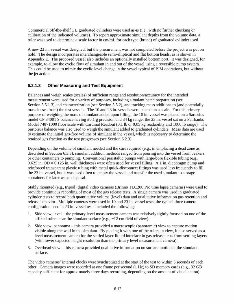
6.12
Commercial off-the-shelf 1 L graduated cylinders were used as-is (i.e., with no further checking or
calibration of the indicated volumes). To report approximate simulant depths from the volume data, a
ruler was used to determine a scale factor in cm/mL for each type (brand) of graduated cylinder used.
A new 23 in. vessel was designed, but the procurement was not completed before the project was put on
hold. The design incorporates interchangeable semi-elliptical and flat bottom heads, as is shown in
Appendix E. The proposed vessel also includes an optionally installed bottom port. It was designed, for
example, to allow the cyclic flow of simulant in and out of the vessel using a reversible pump system.
This could be used to mimic the cyclic level change in the vessel typical of PJM operations, but without
the jet action.
6.2.1.3 Other Measuring and Test Equipment
Balances and weigh scales (scales) of sufficient range and resolution/accuracy for the intended
measurement were used for a variety of purposes, including simulant batch preparation (see
Section 5.5.1.3) and characterization (see Section 5.5.2), and tracking mass additions to (and potentially
mass losses from) the test vessels. The 10 and 23 in. vessels were placed on a scale. For this primary
purpose of weighing the mass of simulant added upon filling, the 10 in. vessel was placed on a Sartorius
model CP 34001 S balance having ±0.1 g precision and 34 kg range; the 23 in. vessel sat on a Fairbanks
Model 748×1000 floor scale with Cardinal Readout (0.1 lb or 0.05 kg readability and 1000 lb range). The
Sartorius balance was also used to weigh the simulant added to graduated cylinders. Mass data are used
to estimate the initial gas-free volume of simulant in the vessel, which is necessary to determine the
retained gas fraction as the test progresses (see Section 6.2.3).
Depending on the volume of simulant needed and the care required (e.g., in emplacing a dead zone as
described in Section 6.3.3), simulant addition methods ranged from pouring into the vessel from beakers
or other containers to pumping. Conventional peristaltic pumps with large-bore flexible tubing (e.g.,
0.625 in. OD × 0.125 in. wall thickness) were often used for vessel filling. A 1 in. diaphragm pump and
reinforced transparent plastic tubing with metal quick-disconnect fittings was used less frequently to fill
the 23 in. vessel, but it was used often to empty the vessel and transfer the used simulant to storage
containers for later waste disposal.
Stably mounted (e.g., tripod) digital video cameras (Brinno TLC200 Pro time lapse cameras) were used to
provide continuous recording of most of the gas release tests. A single camera was used in graduated
cylinder tests to record both quantitative volume (level) data and qualitative information gas retention and
release behavior. Multiple cameras were used in 10 and 23 in. vessel tests; the typical three camera
configuration used in 23 in. vessel tests included the following:
1. Side view, level – the primary level measurement camera was relatively tightly focused on one of the
affixed rulers near the simulant surface (e.g., ~12 cm field of view).
2. Side view, panorama – this camera provided a macroscopic (panoramic) view to capture motion
visible along the wall in the simulant. By placing it with one of the rulers in view, it also served as a
level measurement camera for the settled layer-liquid interface in gas release tests from settling layers
(with lower expected height resolution than the primary level measurement camera).
3. Overhead view – this camera provided qualitative information on surface motion at the simulant
surface.
The video cameras’ internal clocks were synchronized at the start of the test to within 5 seconds of each
other. Camera images were recorded at one frame per second (1 Hz) to SD memory cards (e.g., 32 GB
capacity sufficient for approximately three days recording, depending on the amount of visual action).

6.13
Data on memory cards were uploaded to a personal computer for processing, including preparation of
videos to show events of interest and review of individual frames for surface level vs. time data.
Additional equipment and specialized methods used in testing are described along with results in the
following sections: dead zone test in Section 6.3.3; air-sparger induced gas release tests in Section 6.3.4;
and mechanical agitator-induced gas release tests in Section 6.3.5.
6.2.2 Conducting Tests
This section provides information on the generally applicable approach and methods used in conducting
the spontaneous and induced gas release tests. The tests were similar in most ways and identical in others
(e.g., test vessels and equipment) to RT instability and single simulant layer BC tests conducted by Rassat
et al. (2014). Test instructions, datasheets, and procedures used in that work were informally adapted for
use in the gas release testing reported here.
The test purpose and general planning/scheduling information were communicated by the cognizant
scientist to the test crew either verbally or in writing (e.g., e-mail). Along with a unique test (and/or
simulant batch) I.D. simulant recipes, sample collection and analysis requirements, and simulant filling
targets (i.e., mass, level, and/or volume) were also provided. Data and other test information were
recorded on test-specific bench or data sheets or in Laboratory Record Books, noting the date and time
where relevant. The following are representative test steps and summarize data that were acquired.
Preparatory steps, where applicable, were completed prior to starting the test. These included the
following:
Using the provided recipe, simulant was prepared as described in Section 5.5.1. Depending on
simulant type and other schedule requirements, simulant was typically prepared the day before
testing. Any H2O2 called for in the recipe was withheld until immediately before starting the test (see
below).
Camera clocks and other reference time-pieces were synchronized to within 5 seconds or less
(typically to within 1 to 2 seconds).
The time-lapse cameras were prepared, including labeling and installing memory cards and locating
cameras in final (or near final) positions.
The cleaned and dried vessel was placed on the scale (balance) in a repeatable, earth-level position.
(Optionally, the vessel tare weight was obtained and recorded.)
The scale was tared (zeroed) with the vessel in place in preparation for slurry filling.
Once these steps were completed, vessel filling proceeded as follows:
In some tests, one or more of the cameras were turned on to record the filling process.
H2O2 addition – H2O2 was added and mixed in the container of gas-generating slurry (typically ex
situ). In one settling with gas release test (FG 10-12 in Section 6.4.2), the 10 in. vessel was pre-filled
with slurry following the mass measurement requirements of the vessel filling step below and H2O2
solution was added and mixed in place using a mechanical agitator. (Note that ~80 percent of the
slurry in the dead zone test was non-gas-generating and did not have H2O2 added to it.)
Vessel filling for gas-generating slurry – As soon as practical after H2O2 addition was completed,
slurry was transferred into the vessel to a specified target mass (i.e., gas-free volume equivalent) or to
a target level or volume (e.g., in a graduated cylinder). For the strengths of materials used in these
6.14
tests, the slurry was sufficiently self-leveling that mechanical means were not necessary to flatten and
smooth the surface. Where beneficial and practical, small amounts of simulant smeared or splashed
on the vessel wall above the fill level were removed (e.g., using a spatula and/or a damp towel).
Whether filled to a target mass or volume, the “final” post-cleanup mass of simulant added to the
vessel was measured and recorded. In addition, the start and stop times of the slurry addition were
noted. The fill process typically took ~10 to 15 minutes in the 10 and 23 in. vessels and less in the
graduated cylinders.
Vessel filling for the dead zone test – The steps above for H2O2 addition and filling the gas-generating
slurry are, in general, applicable to dead zone tests. However, because the geometry of the
gas-generating dead zone (e.g., an annular region) was formed during the filling process, the dead
zone slurry and the non-gas-generating bulk slurry had to be added incrementally. In preparation for
filling, the container of non-gas-generating slurry was mixed (e.g., before H2O2 was added to the
other container of slurry). As soon as practical after H2O2 addition was completed, each slurry type
was transferred into the vessel in steps. The mass added in each step was documented so that the
cumulative mass of each type of slurry could be determined and the individual targets met. Because
of the added complexity in defining the dead zone, as well as lack of experience, the fill process in the
23 in. vessel took considerably longer (e.g., ~1 hour) than for bulk addition of gas-generating slurry
only. A more detailed description of the vessel filling process for the dead zone test is provided in
Section 6.3.3.
Initial surface levels – In all test types, the slurry surface level was measured as soon as practical after
the filling process was complete. Typically, the level at each ruler on the 10 and 23 in. vessels was
recorded. The initial volume was recorded instead of level in graduated cylinder tests.
Effectively, the test started once the filling process was finished. Test progress was monitored and tests
were completed as follows:
Cameras – If not done so already, cameras were adjusted to their final positions and recording was
started. The cameras were operated throughout the test, except when stopped to (rarely) adjust the
camera, or to check remaining storage capacity of or switch out memory cards.
Staff operations – One or more staff monitored the test progress intermittently, recording the surface
level/time and other observations (e.g., slurry-liquid interface level and information on visible
bubbles). Around-the-clock staff coverage of the experiments was not used, because the cameras
monitored test progress continuously.
Duration and completion –Test completion was typically defined by the time of the first
instability/GRE, if known, plus an additional period (e.g., 8 hours or more) to track potential
follow-on gas-release events. The duration of an experiment varied due to numerous factors such as
the gas generation rate and the retained gas fraction at the point of the GRE. The cameras were
normally left on until the memory cards were full (~3 days), at which point gas generation had slowed
or stopped due to depleted H2O2.
Cleanup – At the completion of a test, the vessel contents were emptied into a large volume plastic
storage tote (or 5 gal buckets, for smaller quantities) for future waste disposal, and the vessel was
cleaned with water.
6.2.3 Data Analysis
Both qualitative and quantitative data were acquired in the spontaneous and induced gas release tests.
Qualitative data of interest include the nature and extent of slurry motion during an instability/GRE and
6.15
the characteristics/mechanisms of gas release (e.g., BC or BD). The qualitative data were visual,
observed directly by staff and/or recorded by video cameras.
Surface level (or volume) vs. time data were used to quantify changes in the volume of retained gas in
periods of gas retention and resulting from gas releases. Using the level data in conjunction with the
initial fill data, the gas volume changes can be expressed in terms of changes in retained gas volume
fraction in the bulk simulant, Δα. Initial fill data were also used to estimate the initial gas volume
retained in the slurry upon completion of filling, which allowed estimation of the absolute retained gas
volume and volume fraction, α (i.e., gas volume/gaseous slurry volume), as a function of time. These
were the primary quantitative data derived from test measurements. In addition, the bulk retained gas
volume determined as above could be used to estimate α in a dead zone (see Section 6.3.3) or a settled
layer (see Section 6.4.2), assuming that all gas was retained in the specific region. Measurements of the
settled layer level (or equivalent volume) were also required to estimate the settled layer-specific α.
Similarly, the initial dead zone volume, which could be estimated from fill mass and slurry density, was
needed to calculate the dead zone-specific α.
More specific information on data sources, quantification, and use follow. The discussion is written
primarily for 10 and 23 in. vessels, for which volumes are calculated from measured levels. The process
is equally applicable to graduated cylinder tests except that volumes are measured directly and conversion
from level data is not required (and ignored in the following).
Camera level data – Individual frame images obtained from the primary level measurement camera
recordings were the main source of level vs. time data. Staff reviewed video footage and recorded the
data electronically (e.g., in a Microsoft Excel® spreadsheet) for subsequent gas fraction calculations.
The frequency of recorded level data was commensurate with the rate of change of level and/or
interest in events. Level was measured to the nearest 1 mm (the ruler resolution), or 0.5 mm if
discernable, for 10 and 23 in. vessels or interpolated to the nearest 1 mL for graduated cylinders
(10 mL scale increments).
Other level data – Level measurements logged by staff during the test were used to supplement the
camera data. The manual observations also provided in-process α estimates before camera data were
available.
Bulk simulant and settled layer volumes – These were measured directly from graduated cylinders.
For the 10 and 23 in. vessels, the level-volume correlations given in Section 6.2.1 were applied to the
surface level data to determine the bulk simulant volume, including any retained gas, and to the
settled layer level data (if any) for its gaseous volume.
Initial gas-free slurry volume – The initial gas-free slurry volume was estimated as the product of the
mass of simulant added to the vessel and the theoretical gas-free slurry density calculated using
Eq. 5.12 in Section 5.5.2.2. Alternatively, gas-free slurry densities measured on slurry samples at the
same solids concentration, but without H2O2, could be used, if available. These data were not
routinely collected in these preliminary studies, and, therefore, theoretical density was used for
consistency.
Initial gas volume – The initial volume of gas at the completion of filling and first level
measurements was calculated as the difference of the initial bulk simulant volume, calculated from
the measured initial surface level, and the initial gas-free slurry volume.
Total retained gas volume as a function of time – Most directly, the total retained gas volume at any
time was calculated as the difference of the bulk simulant volume, calculated from the level data, and
the estimated initial gas-free slurry volume. An equivalent alternative is to separately determine the
change in bulk slurry volume from the initial measured bulk value (calculated from the initial surface
level) and sum it with the estimated initial gas volume.
6.16
Retained gas volume fraction, α – The retained gas volume fraction is defined as α = Vg/(Vg + VS),
where Vg is the gas volume and VS is the gas-free slurry (simulant) volume. If the bulk average α is to
be determined, the denominator is the gaseous bulk slurry volume (at any time) calculated from the
surface level. Similarly, if the settled layer α is to be determined, the denominator is the gaseous
settled layer volume calculated from the settled layer-liquid interface level. For the dead
zone-specific α, VS is the initial volume of the gas-free dead zone.
Uncertainty – No formal uncertainty analysis was completed for these preliminary studies. At a bare
minimum, it can be determined from the level or volume resolution (readability) of the vessels. For
example, in the 23 in. vessel at the 0.8 H/D fill level that was typically used (~47 cm), the uncertainty
in calculated volume for a 1 mm level measurement resolution is 0.2 percent. Even neglecting
necessary corrections and other contributors to uncertainty, this is an overly optimistic estimate
because of difficulty in accurately reading surface levels in many cases. For example, in
non-Newtonian simulant tests, the surface was generally flat, but not likely uniform to the nearest
1 mm (depending on slurry strength), and a “film” of simulant sometimes developed along the wall at
the surface and hindered level measurement. In similar experiments in the 23 in. vessel, but using a
layer of relatively easy-to-read supernatant water atop a (thinner) layer of slurry simulant, Rassat et
al. (2014) estimated representative uncertainties in α of 1 to 2 vol%. Their gas fraction estimates
included corrections for other sources of error and uncertainty including: initial mass measurements
and evaporative losses; slurry density measurements; and parallax (and refraction) error associated
with the use of a video camera that was not always level with (centered on) the varying surface level
being evaluated. However, their base level measurement uncertainty was higher because the test
vessel was nominally filled to only 0.34 instead of 0.8 H/D. All things considered, an uncertainty in α
of ~2 vol% may be appropriate for the test results reported here.
6.3 Spontaneous and Induced Gas Releases from Non-Newtonian Simulants
Section 6.3.2 provides a test matrix for and an overview of the spontaneous and induced gas release tests
that were completed using non-settling non-Newtonian simulants. These preliminary investigations
included a dead zone spontaneous gas release test (Section 6.3.3) and tests of gas release induced by a
single air sparger (Section 6.3.4) and a mechanical agitator (Section 6.3.5). Objectives and success
criteria that were developed as part of the planning for this effort are given in the following section. In
addition to the objectives noted below, Test Objective 11 in Section 6.1.1 for BC gas releases is also
applicable.
6.3.1 Objectives and Success Criteria
TP-WTPSP-1401 identifies the following test objectives for the effort on quantifying spontaneous gas
releases:
Test Objective 10 - Dead Zone Motion: Quantify and visually characterize gas retention and release
associated with gas retained in un-mixed or imperfectly mixed dead zones of varying shape, volume,
and location in nominally 23 in. and 43 in. diameter vessels using physical simulants for which
spontaneous BC gas releases have been evaluated independently. Assess the effect of mixing and/or
bulk fluid motion, ranging from quiescent to operating PJMs in the 43 in. vessel, on dead zone gas
retention and release behavior for select simulants and dead zone configurations to demonstrate that
measurements in quiescent systems conservatively bound the dead zone gas release hazard.
1 Gauglitz PA. 2015. Test Plan for Hydrogen Gas Release from Vessels Technical Issue Support.
TP-WTPSP-140, Rev. 0, Pacific Northwest National Laboratory.
6.17
Test Objective 12 - Buoyant Displacement Gas Release Events: Measure the retained gas fraction in
non-Newtonian slurry simulant at the onset of spontaneous BDGREs in the presence of a relatively
thick supernatant liquid layer for a range of simulant rheology (e.g., shear strength and Bingham yield
stress) that is representative of those anticipated for WTP waste streams. Also investigate the effect
of sediment layer depth to evaluate existing theory on how the gas fraction at the onset of a BDGRE
may exceed neutral buoyancy depending on the strength and thickness of the sediment layer.
The following criteria were to be used to assess the successful completion of Test Objective 10:
measure retained gas fraction as a function of time through the onset of dead zone motion
measure the shear strength and Bingham yield stress and consistency for the non-Newtonian simulant
compositions used in dead zone motion testing
establish a level-volume correlation for each test vessel.
The following criteria were to be used to assess the successful completing of Test Objective 12:
measure retained gas fraction as a function of time through the BDGRE
for each BDGRE test, determine the theoretical neutral buoyancy gas fraction and compare to the
measured gas fraction to assess how much the gas fraction exceeds neutral buoyancy
measure the shear strength and Bingham yield stress and consistency for the non-Newtonian simulant
compositions used in gas release testing
establish a level-volume correlation for each test vessel.
6.3.2 Test Overview
As suggested by Objective 10 above, plans called for dead zone gas release tests in non-Newtonian
simulants using dead zones of varying shape, volume, and location in multiple vessels, both under
quiescent conditions and with mixing. The quiescent dead zone test discussed in the following section
was the only spontaneous gas release test conducted using non-settling non-Newtonian simulant in the
preliminary studies covered by this report. (Spontaneous gas releases from settling layers of low-solids
simulants are discussed in Section 6.4.) The dead zone test was successful with respect to success criteria
for Objective 10. However, interpretation of the results is limited to some extent because the supporting
baseline BD tests (Objective 12 in Section 6.3.1) and BC tests (Objective 11 in Section 6.1.1), in
particular, had not been initiated at the time the flammable-gas testing tasks were shut down.
Early in project planning, induced gas release testing in 10 and 23 in. vessels, such as that presented here,
was considered a possible means to evaluate and compare head-to-head the gas release behavior of
various simulants. This relatively large-scale approach of simulant evaluation leading to simulant
selection is not specifically identified in the objectives and success criteria in the previous section,
because alternate methods (e.g., those proposed in Section 5.2 and depicted schematically in Figure 5.1)
were chosen and included in test plan. That approach uses much smaller volumes of simulant, making it
more amenable to use with actual waste for direct comparison of gas release behavior. The induced gas
release tests described in this section fall in the category “Single Static Release Following Generation”
defined in Section 5.2, as opposed to “Continuous Generation and Release Under Shear.” The shakedown
gas release test that was conducted as part of early mixing metric/requirement studies (see
Section 3.5.1.2) also used the single bulk H2O2 addition method and the same 23 in. vessel as the
air-sparger-induced gas release tests described below (Section 6.3.4), but used mechanical agitation to
induce release. This is analogous to the shaft mixer tests completed in the 10 in. vessel that are discussed
briefly in Section 6.3.5.
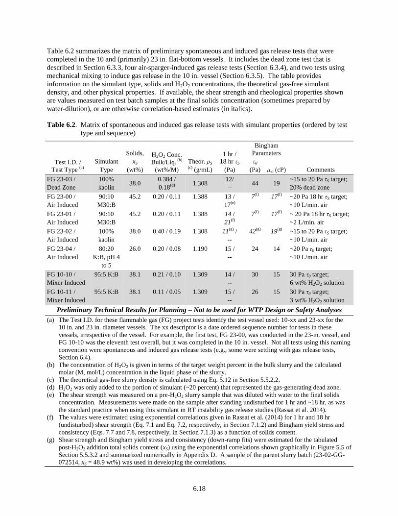
6.18
Table 6.2 summarizes the matrix of preliminary spontaneous and induced gas release tests that were
completed in the 10 and (primarily) 23 in. flat-bottom vessels. It includes the dead zone test that is
described in Section 6.3.3, four air-sparger-induced gas release tests (Section 6.3.4), and two tests using
mechanical mixing to induce gas release in the 10 in. vessel (Section 6.3.5). The table provides
information on the simulant type, solids and H2O2 concentrations, the theoretical gas-free simulant
density, and other physical properties. If available, the shear strength and rheological properties shown
are values measured on test batch samples at the final solids concentration (sometimes prepared by
water-dilution), or are otherwise correlation-based estimates (in italics).
Table 6.2. Matrix of spontaneous and induced gas release tests with simulant properties (ordered by test
type and sequence)
Test I.D. /
Test Type (a)
Simulant
Type
Solids,
xS
(wt%)
H2O2 Conc.
Bulk/Liq. (b)
(wt%/M)
Theor. ρS (c)
(g/mL)
1 hr /
18 hr τS
(Pa)
Bingham
Parameters
Comments
τ0
(Pa) μ∞ (cP)
FG 23-03 /
Dead Zone
100%
kaolin 38.0
0.384 /
0.18(d)
1.308
12/
-- 44 19
~15 to 20 Pa τS target;
20% dead zone
FG 23-00 /
Air Induced
90:10
M30:B
45.2 0.20 / 0.11 1.388 13 /
17(e)
7(f)
17(f)
~20 Pa 18 hr τS target;
~10 L/min. air
FG 23-01 /
Air Induced
90:10
M30:B
45.2 0.20 / 0.11 1.388 14 /
21(f)
7(f)
17(f)
~ 20 Pa 18 hr τS target;
~2 L/min. air
FG 23-02 /
Air Induced
100%
kaolin
38.0 0.40 / 0.19 1.308 11(g)
/
--
42(g)
19(g)
~15 to 20 Pa τS target;
~10 L/min. air
FG 23-04 /
Air Induced
80:20
K:B, pH 4
to 5
26.0 0.20 / 0.08 1.190 15 /
--
24 14 ~20 Pa τ0 target;
~10 L/min. air
FG 10-10 /
Mixer Induced
95:5 K:B 38.1 0.21 / 0.10 1.309 14 /
--
30 15 30 Pa τ0 target;
6 wt% H2O2 solution
FG 10-11 /
Mixer Induced
95:5 K:B 38.1 0.11 / 0.05 1.309 15 /
--
26 15 30 Pa τ0 target;
3 wt% H2O2 solution
Preliminary Technical Results for Planning – Not to be used for WTP Design or Safety Analyses
(a) The Test I.D. for these flammable gas (FG) project tests identify the test vessel used: 10-xx and 23-xx for the
10 in. and 23 in. diameter vessels. The xx descriptor is a date ordered sequence number for tests in these
vessels, irrespective of the vessel. For example, the first test, FG 23-00, was conducted in the 23-in. vessel, and
FG 10-10 was the eleventh test overall, but it was completed in the 10 in. vessel. Not all tests using this naming
convention were spontaneous and induced gas release tests (e.g., some were settling with gas release tests,
Section 6.4).
(b) The concentration of H2O2 is given in terms of the target weight percent in the bulk slurry and the calculated
molar (M, mol/L) concentration in the liquid phase of the slurry.
(c) The theoretical gas-free slurry density is calculated using Eq. 5.12 in Section 5.5.2.2.
(d) H2O2 was only added to the portion of simulant (~20 percent) that represented the gas-generating dead zone.
(e) The shear strength was measured on a pre-H2O2 slurry sample that was diluted with water to the final solids
concentration. Measurements were made on the sample after standing undisturbed for 1 hr and ~18 hr, as was
the standard practice when using this simulant in RT instability gas release studies (Rassat et al. 2014).
(f) The values were estimated using exponential correlations given in Rassat et al. (2014) for 1 hr and 18 hr
(undisturbed) shear strength (Eq. 7.1 and Eq. 7.2, respectively, in Section 7.1.2) and Bingham yield stress and
consistency (Eqs. 7.7 and 7.8, respectively, in Section 7.1.3) as a function of solids content.
(g) Shear strength and Bingham yield stress and consistency (down-ramp fits) were estimated for the tabulated
post-H2O2 addition total solids content (xS) using the exponential correlations shown graphically in Figure 5.5 of
Section 5.5.3.2 and summarized numerically in Appendix D. A sample of the parent slurry batch (23-02-GG-
072514, xS = 48.9 wt%) was used in developing the correlations.

6.19
6.3.3 Gas Release from a Dead Zone
The possible locations, shapes, sizes, and strengths of dead zones in WTP process vessels are numerous.
Figure 6.7 (left) is a schematic representation of postulated “batwing” dead zones of three different sizes
forming at the bottom of a vessel between PJM regions of influence. Another possible scenario is for
dead zones forming in the shadow of PJMs, between the PJM bodies and the vessel wall. Figure 6.7
(right) shows a highly-simplified dead zone experimental concept used in Test FG 23-03: it is a
partial-height annular gas-generating dead zone of ~20 percent of the initial slurry volume with an overall
fill height of ~0.8 height-to-diameter (H/D) ratio in a 23 in. diameter vessel.
Figure 6.7. Schematic drawings of (left) “batwing” dead zones of three sizes formed between PJM
regions of influence and (right) the partial-height annular gas-generating dead zone used in
Test FG 23-03
In this first dead zone test, as is depicted in the schematic drawing, the dead zone slurry was dyed blue
and contained H2O2 to generate gas bubbles. The dead zone was surrounded by un-dyed
non-gas-generating slurry of nominally the same composition, gas-free density, and strength
(τS = 12 Pa and τ0 = 44 Pa; see Table 6.2). A 5 gal plastic bucket (~10.5 to 11 in. [~27 to 28 cm]
diameter) with the bottom cutoff was used as a jig to setup the annular dead zone geometry, as follows. A
layer of duct tape was wrapped around the bottom perimeter of the bucket leaving a narrow strip
unattached at the bottom. The bucket was then set, approximately centered, on the bottom of the vessel,
using the tape to help hold it loosely in place (for ease in removing it later). The tape also acted
somewhat as a gasket in minimizing the radial flow of slurry under the bucket during loading. H2O2 was
added to the dead zone slurry stock within minutes of starting the fill process. To help further minimize
slurry flow under the bucket, the addition of non-gas-generating slurry inside and gas-generating slurry
outside the bucket was staggered to reduce the differential head. After the target mass of dead zone slurry
was added in the annular region (using a handheld scoop and a peristaltic pump), filling the non-dead
zone slurry continued with the bucket in place in both the center and on top of the dyed dead zone slurry
in the annulus. Care was taken to try to maintain a flat (horizontal) interface between the dyed and
un-dyed slurry, but the slurry was too weak to do this cleanly, which was indicated by the spread of a film
of dyed slurry up the wall above the initial fill height. After the dead zone was completely covered by a
layer of un-dyed slurry of at least 2 cm, the bucket was removed by pulling it straight up. The remainder
Gas Release
from
Dead Zones

6.20
of the non-gas-generating slurry was then added by mass,1 initial slurry levels were recorded, and the test
was underway. Changes in slurry level were recorded continually by a video camera to determine
retained gas fractions and assess the size of any spontaneous GREs.
It was expected that gas would be retained in the initially neutrally buoyant dead zone slurry until either
the gas fraction was sufficiently high to overcome the strength of the surrounding non-dead zone slurry
and allow it to rise buoyantly in bulk (e.g., gaseous slurry “gobs”) or until the gas fraction necessary for
the onset of a spontaneous BC from the dead zone slurry was reached (see Section 6.1.4.3). Additional
video cameras were used to provide qualitative information to help evaluate if gas retention and release
from the dead zone followed this anticipated physical behavior. Figure 6.8 shows a time sequence of top
and side view video still images (photos) for the dead zone test. Images are shown for 1 second before
any observed motion, ~2 seconds after motion was detected at the side of the vessel, and ~17 seconds
following the start of the event and after motion and gas release essentially stopped (visually). Before
motion was observed (left-side images in Figure 6.8), the top surface of un-dyed slurry was flat and
showed no evidence of dead zone migration or gas release (e.g., no dyed slurry or pock marks). Except
for some increase in level due to gas retention, the pre-event side view image appears much the same as it
did at the start of the test. The irregularity of the dead zone /bulk slurry interface is primarily (if not
entirely) due to distortion from the filling process, as discussed above. The middle images of Figure 6.8
show the rapid transition from the quiescent pre-event state to a highly energetic (appearing) state of
significant buoyant motion. Both the top and side view photos show an up-well of dyed slurry, which is
apparent in a single large (~half the vessel diameter) bubble/slurry mass cresting at the surface. The
middle side view image in Figure 6.8 also shows streaking of dyed clay at the wall near the surface and a
slight decrease in level of the dead zone/bulk slurry interface (right side of photo); however the shape and
height of the interface is largely unchanged on the left side. A few smaller up-well releases were
observed at the surface for another ~10 seconds in an area surrounding the initial epicenter. The right-
hand images in Figure 6.8 show the “final” result of the GRE. More than half the surface was covered
with dyed dead zone slurry, which was carried in and spread away from upwell regions. In addition, dyed
slurry extended higher up the vessel wall from the bottom (right side of image on the lower right)
compared to earlier times, which may indicate that more-dense bulk slurry replaced and pushed up
remaining gas-containing dead zone slurry near the bottom of the vessel.
Although visually dramatic, the buoyant motion of the dead zone did not result in significant quantities of
released gas. Figure 6.9 shows the retained gas volume fraction as function of time starting from
completion of the slurry filling process. The gas fraction was determined from changes in surface level,
which reflects gas retained on average by the bulk of the slurry. The figure shows both the bulk average α
and the calculated gas fraction in the dead zone, assuming that all the generated gas was retained in the
volume of initially gas-free dead zone, which was 20 percent of the total. The GRE, identified by a
vertical line and labeled as an instability event in Figure 6.9, occurred after 15 hours at a bulk average α
of 4.6 vol% and a dead zone-specific α of 19 vol%. It is estimated that only 9 percent of the retained gas
was released in the GRE (a 2 mm drop in the ~48 cm level). After the GRE, gas continued to be
generated and retained, reaching a maximum bulk α of 5.2 vol% (21 vol% as dead zone-specific) at
~23 hours, after which α leveled out and slowly decayed. It is unknown whether gas continued to be
generated after the peak α was reached. Stoichiometrically, sufficient H2O2 was added to achieve
>60 vol% α in the dead zone; however as noted in Section 5.5.3.3, kaolin and high kaolin fraction K:B
slurries (e.g., 98:2 K:B) have been shown to generate significantly less than the theoretical amount of
oxygen. Also note that the construct of a dead zone-specific α becomes non-physical after the GRE,
because the dead zone and bulk slurries are blended to some extent.
1 Because of unanticipated losses in readying a diaphragm pump that was not used, insufficient non-gas-generating
slurry was available to meet the exact target mass. The final mass ratio was 79.4 percent bulk to 20.6 percent dead
zone, minimally different than the target 80/20 split.
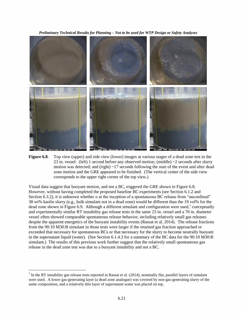
6.21
Preliminary Technical Results for Planning – Not to be used for WTP Design or Safety Analyses
Figure 6.8. Top view (upper) and side view (lower) images at various stages of a dead zone test in the
23 in. vessel: (left) 1 second before any observed motion; (middle) ~2 seconds after slurry
motion was detected; and (right) ~17 seconds following the start of the event and after dead
zone motion and the GRE appeared to be finished. (The vertical center of the side view
corresponds to the upper right corner of the top view.)
Visual data suggest that buoyant motion, and not a BC, triggered the GRE shown in Figure 6.8.
However, without having completed the proposed baseline BC experiments (see Section 6.1.2 and
Section 6.3.2), it is unknown whether α at the inception of a spontaneous BC release from “unconfined”
38 wt% kaolin slurry (e.g., bulk simulant not in a dead zone) would be different than the 19 vol% for the
dead zone shown in Figure 6.9. Although a different simulant and configuration were used,1 conceptually
and experimentally similar RT instability gas release tests in the same 23 in. vessel and a 70 in. diameter
vessel often showed comparable spontaneous release behavior, including relatively small gas releases
despite the apparent energetics of the buoyant instability events (Rassat et al. 2014). The release fractions
from the 90:10 M30:B simulant in those tests were larger if the retained gas fraction approached or
exceeded that necessary for spontaneous BCs or that necessary for the slurry to become neutrally buoyant
in the supernatant liquid (water). (See Section 6.1.4.3 for a summary of the BC data for the 90:10 M30:B
simulant.) The results of this previous work further suggest that the relatively small spontaneous gas
release in the dead zone test was due to a buoyant instability and not a BC.
1 In the RT instability gas release tests reported in Rassat et al. (2014), nominally flat, parallel layers of simulant
were used. A lower gas-generating layer (a dead zone analogue) was covered by non-gas-generating slurry of the
same composition, and a relatively thin layer of supernatant water was placed on top.
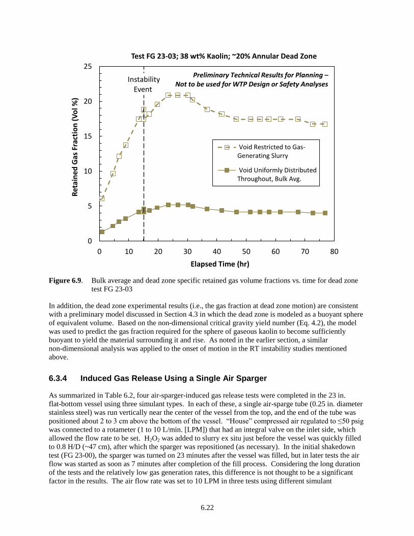
6.22
Figure 6.9. Bulk average and dead zone specific retained gas volume fractions vs. time for dead zone
test FG 23-03
In addition, the dead zone experimental results (i.e., the gas fraction at dead zone motion) are consistent
with a preliminary model discussed in Section 4.3 in which the dead zone is modeled as a buoyant sphere
of equivalent volume. Based on the non-dimensional critical gravity yield number (Eq. 4.2), the model
was used to predict the gas fraction required for the sphere of gaseous kaolin to become sufficiently
buoyant to yield the material surrounding it and rise. As noted in the earlier section, a similar
non-dimensional analysis was applied to the onset of motion in the RT instability studies mentioned
above.
6.3.4 Induced Gas Release Using a Single Air Sparger
As summarized in Table 6.2, four air-sparger-induced gas release tests were completed in the 23 in.
flat-bottom vessel using three simulant types. In each of these, a single air-sparge tube (0.25 in. diameter
stainless steel) was run vertically near the center of the vessel from the top, and the end of the tube was
positioned about 2 to 3 cm above the bottom of the vessel. “House” compressed air regulated to ≤50 psig
was connected to a rotameter (1 to 10 L/min. [LPM]) that had an integral valve on the inlet side, which
allowed the flow rate to be set. H2O2 was added to slurry ex situ just before the vessel was quickly filled
to 0.8 H/D (~47 cm), after which the sparger was repositioned (as necessary). In the initial shakedown
test (FG 23-00), the sparger was turned on 23 minutes after the vessel was filled, but in later tests the air
flow was started as soon as 7 minutes after completion of the fill process. Considering the long duration
of the tests and the relatively low gas generation rates, this difference is not thought to be a significant
factor in the results. The air flow rate was set to 10 LPM in three tests using different simulant
Instability Event
0
5
10
15
20
25
0 10 20 30 40 50 60 70 80
Ret
ain
ed G
as F
ract
ion
(V
ol %
)
Elapsed Time (hr)
Test FG 23-03; 38 wt% Kaolin; ~20% Annular Dead Zone
Void Restricted to Gas-Generating Slurry
Void Uniformly DistributedThroughout, Bulk Avg.
Preliminary Technical Results for Planning –Not to be used for WTP Design or Safety Analyses
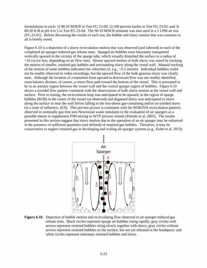
6.23
formulations in each: 1) 90:10 M30:B in Test FG 23-00; 2) 100 percent kaolin in Test FG 23-02; and 3)
80:20 K:B at pH 4 to 5 in Test FG 23-04. The 90:10 M30:B simulant was also used in a 2 LPM air test
(FG 23-01). Before discussing the results of each test, the bubble and slurry motion that was common to
all is briefly noted.
Figure 6.10 is a depiction of a slurry recirculation motion that was observed (and inferred) in each of the
completed air-sparger-induced gas release tests. Sparged air bubbles were buoyantly transported
vertically upward in the vicinity of the sparge tube, which visually disturbed the surface in a radius of
~10 cm (or less, depending on air flow rate). Slower upward motion of bulk slurry was noted by tracking
the motion of smaller, retained gas bubbles and surrounding slurry along the vessel wall. Manual tracking
of the motion of some bubbles indicated rise velocities of, e.g., ~0.5 cm/min. Individual bubbles could
not be readily observed in video recordings, but the upward flow of the bulk gaseous slurry was clearly
seen. Although the location of a transition from upward to downward flow was not readily identified,
mass balance dictates, of course, a return flow path toward the bottom of the vessel. This is presumed to
be in an annular region between the vessel wall and the central sparger region of bubbles. Figure 6.10
shows a toroidal flow pattern consistent with the observations of bulk slurry motion at the vessel wall and
surface. Prior to testing, the recirculation loop was anticipated to be upward, in the region of sparge
bubbles (ROB) in the center of the vessel (as observed) and degassed slurry was anticipated to move
along the surface to near the wall before falling in the less-dense gas-containing and/or un-yielded slurry
(in a zone of influence, ZOI). This pre-test picture is consistent with the ROB/ZOI recirculation patterns
observed in nominally gas-free non-Newtonian waste simulants in the evaluation of air spargers as a
possible means to supplement PJM mixing in WTP process vessels (Poloski et al. 2005). The results
presented in this section suggest that slurry motion due to the operation of an air sparger may be enhanced
in the presence of sufficient quantities (not defined) of retained gas bubbles. Therefore, it may be
conservative to neglect retained gas in developing and scaling air-sparger systems (e.g., Kuhn et al. 2013).
Figure 6.10. Depiction of bubble motion and recirculating flow observed in air-sparger-induced gas
release tests. Black circles represent sparge air bubbles rising rapidly; gray circles with
arrows represent retained bubbles rising slowly together with slurry; gray circles without
arrows represent retained bubbles on the surface, but not yet released to the headspace; and
white circles represent stationary retained bubbles and slurry.
Air
Sparger

6.24
In the experiments that were conducted, there were transient effects in the air-sparger-induced gas release
process. With reference to the well-established recirculation flow patterns depicted in Figure 6.10, the
transient behavior could potentially be interpreted as follows. At early times with lower retained gas
fractions and less of the non-Newtonian slurry yielded, the upward vertical flow would be more restricted
to the sparged center region of the vessel. As more gas was retained and more slurry was yielded (e.g., by
sparger action on bubbly slurry having decreased yield stress with increasing α), the flow patterns would
extend radially outward and progressively include more slurry in the bottom “corner” of the vessel. At the
same time, increased gas retention would make the slurry more buoyant and upward flow along the wall
would increase. Starting from relatively low gas fractions, this process would tend to control the release
rate and prevent large spontaneous releases. This was observed in the experiments described below.
Figure 6.11 shows the retained gas volume fraction in 38 wt% kaolin slurry as a function of time in
Test FG 23-02. For comparison to the air-sparger-induced gas release test, a 1 L graduated cylinder was
filled with a portion of the simulant that was added to the 23 in. vessel. The gas retention profile for the
parallel graduated cylinder test is also shown in Figure 6.11. Based on comparison of these data, the
initial growth rate was not significantly affected by operation of the sparger at an air flow rate of 10 LPM
– although data are sparse for the manually observed graduated cylinder test, the retained gas fractions in
the two vessels appear to track each for the first ~9 hours. Beyond that, the rate of increase in retention
slowed in the 23 in. vessel. It reached a maximum α of 12 vol% shown by the 14 and 21 hour data in
Figure 6.11, after which the retained gas fraction (holdup) slowly decreased, presumably due to operation
of the sparger. As indicated by a vertical line in the figure, the sparger was turned off at 39 hours. It
cannot be determined conclusively that the increase in α at 39 hours is due solely to turning the sparger
off. It is possible that a local minimum in α (e.g., 8 vol%) had been reached and that the level would have
increased even if the sparger had been left on (i.e., turning off the sparger may have coincided with the
minimum). Additional testing with continual operation of the sparger is needed to determine if the
retention profile is cyclic or whether the gas holdup reaches a minimum and holds constant for extended
periods. The limited growth after the sparger was turned off and the steady level after 52 hours is likely
due to the decreased concentration and then complete consumption of the H2O2.
Figure 6.12 shows the retained gas volume fractions in 45.2 wt% 90:10 M30:B simulant, from two
separate batches, as a function time using air sparger flow rates of 2 LPM (Test FG 23-01) and 10 LPM
(Test FG 23-00).1 The H2O2 concentration was 0.20 wt% in both tests, and this is reflected in the
consistent gas generation rates that are inferred from the overlapping retention profiles in Figure 6.12 for
the first hour of the tests. With essentially equal gas generation rates, differences in gas retention and
release behavior shown in the figure can be attributed to differences in operation of the sparger. At
10 LPM air, the peak sparger-on α was ~8 vol% at 2 hours elapsed time, and at 2 LPM air, α peaked at
12 vol% after ~4 hours. In both cases, the retained gas fraction decreased continually and relatively slowly
while the sparger was run for 20 hours. The minimum α values near that point in time were ~3 and
~6 vol% at the higher and lower sparge rates, respectively. As was the case with the kaolin test discussed
above, it cannot be determined whether the retained gas fraction had reached a steady state at the time the
sparger was turned off in the 90:10 M30:B tests shown in Figure 6.12. However, operation of the sparger
appeared to suppress both the peak retention and the rate of subsequent gas release. The latter is discerned
from Figure 6.12 by comparing retention and release behavior in the sparger-on periods to the nearly
instantaneous “secondary” GREs that occurred with the sparger off (e.g., at about 29 and 33 hours).
1 At 23 minutes into Test FG 23-00, the sparger was turned on at 5 LPM before increasing the flow rate to 10 LPM
45 minutes into the test. In Test FG 23-01, the sparger was set to 2 LPM after 16 minutes and held constant.
Turning the sparger on to 10 LPM sooner in Test FG 23-00 may have further limited the peak gas fraction compared
to the 2 LPM air test.

6.25
Figure 6.11. Retained gas volume fraction vs. time in air-sparger-induced gas release Test FG 23-02
compared to a parallel test of retention of the same batch of 38 wt% kaolin simulant in a
graduated cylinder. (The graduated cylinder data point at 60 hours is not connected by a
line so that the gas release is not portrayed, unknowingly, as a slow process, which would
not be expected.)
Figure 6.12. Retained gas volume fractions in 45.2 wt% 90:10 M30:B simulant as a function time using
air sparger flow rates of 2 LPM (Test FG 23-01) and 10 LPM (Test FG 23-01)
Sparger Off
0
10
20
30
40
50
0 10 20 30 40 50 60 70
Ret
ain
ed
Gas
Fra
ctio
n (
Vo
l %)
Elapsed Time (hr)
Test FG 23-02
Graduated Cylinder, Parallel Test
Preliminary Technical Results for Planning – Not to be used for WTP Design or Safety Analyses
Sparger Off
0
5
10
15
20
0 10 20 30 40 50 60
Ret
ain
ed
Gas
Fra
ctio
n (
Vo
l %)
Elapsed Time (hr)
Test FG 23-00, 10 LPM air
Test FG 23-01, 2 LPM air
Preliminary Technical Results for Planning – Not to be used for WTP Design or Safety Analyses
6.26
The results of previous spontaneous BC gas release tests using the same 90:10 M30:B simulant are
summarized in Section 6.4. The data included there are for the peak retention preceding first spontaneous
GREs, which were larger, both in quantity retained and released, than secondary events (Rassat et al.
2014). For example, Table 6.1 shows that spontaneous BCs occurred at α of about 30 vol% and that
>95 percent of the retained gas was released (almost instantaneously) for 90:10 M30:B simulant having
estimated shear strength of 16 and 26 Pa at the time of the GRE. Compared to this earlier work, the
greater secondary retention and larger releases shown in Figure 6.12 after the sparger was turned off (after
20 hours in each test) provides further evidence that operation of the sparger both limited the peak gas
holdup and dampened the release rate. In summary, the data suggest that continuous operation of air
spargers, even at relatively low flow rates, may be effective in helping to mitigate large spontaneous gas
releases; however, this behavior is probably specific to the relatively uniform non-Newtonian slurry
evaluated in these tests.
Figure 6.13 compares retained gas volume fractions in 10 LPM air sparger tests using three simulant
types. Results for 38 wt% kaolin (Test FG 23-02) are reproduced from Figure 6.11. Likewise, results for
45.2 wt% 90:10 M30:B (Test FG 23-00) from Figure 6.12 are shown again in Figure 6.13. New data are
included for 26 wt% 80:20 K:B at pH 4 to 5 (Test FG 23-04). Consistent with the tests discussed earlier,
gas retention in Test FG 23-04 increased from the start even with the sparger on, reaching an initial peak
α of ~7 vol% in about 4 hours before decaying slowly to 3.5 vol% over 44 hours when the sparger was
turned off. The results are also similar in that the retained gas fraction increased immediately after
turning off the sparger (which occurred at different times in the three tests). In all cases, this was an
indicator that lower α values at longer times did not result from a lack of gas generation due to complete
consumption of H2O2. The differences in peak gas retention and release behavior shown in Figure 6.13
may be a function of the physical properties of the simulants. As shown in Table 6.2, the 1 hour shear
strengths1 and the Bingham consistencies of these simulants were measured or estimated to vary over
fairly narrow ranges (τS = 11 to 15 Pa and μ∞ = 14 to 19 cP). However, the range of yield stresses was
much larger at 7 to 42 Pa (i.e., 7 Pa for the 90:10 M30:B, 24 Pa for the 80:20 K:B at pH 4 to 5, and 42 Pa
for the pure kaolin). In the periods that the sparger was on, kaolin had the highest retained gas fraction at
~12 vol% while the other two peaked in the ~7 to 8 vol% range. The high value for kaolin might be
explained by its high yield stress, but the relatively low result for 80:20 K:B at pH 4 to 5 is not.
Given that the recirculation flow depicted in Figure 6.10 is buoyancy driven, slurry density is also likely
to play a role in the trends shown in Figure 6.13. For example, comparing the pH adjusted 80:20 K:B
(ρS = 1.19 g/mL, τ0 = 24 Pa) to the 90:10 M30:B (ρS = 1.39 g/mL, τ0 = 7 Pa), the higher yield stress of the
first, which would tend to restrict fluid motion, may be compensated for by its relatively low density,
which makes it more buoyant at lower retained gas fractions.
Differences in gas retention and release behavior shown in Figure 6.13 may also arise from differences in
gas generation rates in the three simulants. These differences are apparent in the first few hours of each
test. As noted in the discussion of Figure 6.11, the initial growth rate in the kaolin test (at least) was not
diminished by operation of the sparger. The results in Figure 6.13 indicate that the gas generation rate
was fastest in 90:10 M30:B and slowest in kaolin, with pH adjusted 80:20 K:B falling in the middle. This
was true even though the concentration of H2O2 was twice as high in the kaolin test (see Table 6.2) and
the 80:20 K:B was acidified to retard its generation rate (see Section 5.5.3.3). Because the peak retained
gas fractions with the sparger turned on were similar for the 90:10 M30:B and the 80:20 K:B, despite the
faster generation rate in the 90:10 M30:B, the higher initial maximum α in kaolin cannot be attributed to
its relatively slow gas generation alone.
1 For the portions of the induced gas release experiments in which the spargers were on and (at least some) slurry
was motion, the 1 hour undisturbed τS is more relevant than the 18 hour undisturbed result. This distinction is most
significant for 90:10 M30:B simulant, which shows considerable time dependence in τS (Rassat et al. 2014).

6.27
Figure 6.13. Comparison of retained gas volume fractions in air-sparger-induced gas release tests at
10 LPM using three simulant types
Data for Test FG 23-04 in Figure 6.13, which was started on a Friday and run over the weekend, are
sparse for long periods after the initial peak in α, because a film of simulant was left on the wall as the
level receded and made reading the level difficult. The data at 27 and 44 hours were taken after carefully
scraping the wall with a spatula in the immediate vicinity of the level measurement ruler and camera. The
film buildup was worse for the pH adjusted 80:20 K:B than for the other two simulant types used in the
sparger tests, but it was only an issue when the level was decreasing. This difficulty was also noted in
tests using 95:5 K:B discussed in the next section.
6.3.5 Induced Gas Release Using Mechanical Agitators
As noted in Section 6.3.2, induced gas release testing in 10 and 23 in. vessels was considered a possible
means for a head-to-head comparison of the gas release behavior of various simulant types or varying
simulant properties. This section briefly outlines two preliminary mechanical-agitator induced gas release
tests that were completed in the 10 in. vessel with the primary purpose of evaluating the potential utility
of such an approach. Gas generation rate was the only intended variable in the tests. To minimize
variability in simulant batch preparation and simulant rheological properties, a double-batch of 95:5 K:B
simulant stock was prepared for use in both tests. In addition, the same mass fraction of H2O2 solution
was added to obtain to the final solids concentration (i.e., 38.1 wt% as shown in Table 6.2). Only the
concentration of the H2O2 stock was varied, with the intended result of affecting gas generation rate
through a ~two-fold difference in the final concentration of H2O2 in the slurry: nominally 6 wt% H2O2
solution was used in Test FG 10-10 for a target 0.21 wt% H2O2 in the slurry and 3.3 wt% H2O2 solution
was used in Test FG 10-11 for a target 0.11 wt% H2O2 in the slurry.
Sparger Off23-00 Sparger Off
23-02
Sparger Off23-04
0
5
10
15
20
0 10 20 30 40 50 60
Ret
ain
ed
Gas
Fra
ctio
n (
Vo
l %)
Elapsed Time (hr)
FG 23-00: 45.2 wt% 90:10 M30:B
FG 23-02: 38 wt% Kaolin
FG 23-04: 26 wt% 80:20 K:B, pH 4 to 5
Preliminary Technical Results for Planning –Not to be used for WTP Design or Safety Analyses
6.28
Immediately following addition of H2O2 to approximately half of the stock slurry, the 10 in. vessel was
filled to a target 1.0 H/D fill level (~25 cm). A shaft mixer with a ~8 cm diameter trefoil-geometry
impeller (oriented for down-flow) was located ~2 to 3 cm above the bottom of and centered in the vessel.
As soon as practical after filling the vessel (5 to 7 minutes in the two tests), the mixer was started at
~500 rpm. This speed was determined in preliminary tests with available gas-free 80:20 K:B slurry
(similar to that used in the test discussed in Section 3.5.1.2) to induce minimal surface motion and only in
the vicinity of the mixer shaft. In the gas release tests, gas bubbles (some >1 cm diameter) were released
near the mixer shaft almost immediately after turning on the motor. Surface motion was initially confined
to near the mixer shaft, but over time, the surface motion spread radially outward. In Test FG 10-10, very
slow surface motion was seen almost to the wall, and in Test FG 10-11, the motion substantially stopped
~4 to 5 cm away from the wall. In both cases, the surface became highly irregular (i.e., “cracked” and
non-flat) and pock-marked from released bubbles and the level was significantly depressed (e.g., ~1 cm or
more) toward the center of the vessel where slurry was yielded. These factors and associated buildup of
clay along the wall rendered quantification essentially useless, especially from the perspective of a 1 mm
level measurement resolution goal. This experimental challenge might be overcome by inclusion of a
relatively thin (e.g., 3 to 5 cm) layer of supernatant liquid. However, possible incorporation of the liquid
in the slurry would also negate the goal of testing at fixed rheological properties.
One L graduated cylinder gas generation (gas retention) rate tests were run in parallel with the 10 in. vessel
tests, in similar fashion to that depicted in and discussed with Figure 6.11. The manual level observation
data indicate that the gas generation rates over the first 2 hours, at least, were inexplicably higher for the
slurry having the lower concentration of H2O2. While an experimental error may have occurred, care was
taken to use the correct H2O2 stock solutions and recorded lot numbers indicate those solutions were
correct. As noted in the simulant materials discussion in Section 5.5.1.1, we had no previous experience
using the 6 wt% H2O2 solution before this project, and it is unknown if it contained additives that would
stabilize and retard gas generation. Further investigation is warranted before using it in a quantitative way.
6.4 Spontaneous Gas Releases from Settling Solids Layers
Retention and release during settling is preliminarily addressed in this report through both analyses and
supporting testing. Results of baseline BC and BD spontaneous gas release tests outlined as objectives in
Section 6.3.1 would provide information to compare to, and possibly refine, the models for gas release
behavior from settled beds (see Section 7.0). These baseline BC and BD tests differ from the tests
described in this section because the baseline tests would establish settled solids layers as the initial
condition in experiments. The tests described in this section are intended to confirm that similar gas
release behavior is observed from settled layers when these layers are formed in situ. The results of these
tests are also more directly comparable to some model calculations (Section 7.2). In the following
sections, the objective and success criteria developed as part of the planning for the experimental effort
are given before describing the settling with gas release tests.
6.4.1 Objectives and Success Criteria
TP-WTPSP-1401 identifies the following test objective for the effort on quantifying spontaneous gas
releases from settling solids layers:
Test Objective 16 – Demonstrate Gas Retention and Release during Settling: Demonstrate gas
retention and release from a settling (in situ settled) bed of simulant solids representing a post-DBE
scenario in WTP low-solids vessels for comparison to model predictions. Conduct experiments using
1 Gauglitz PA. 2015. Test Plan for Hydrogen Gas Release from Vessels Technical Issue Support. TP-WTPSP-
140, Rev. 0, Pacific Northwest National Laboratory.

6.29
a range of initial simulant solids concentrations and nominally similar gas generation rates. For at
least one solids concentration, evaluate the effect of gas generation rate and, separately, use an
alternate supernatant liquid having a different density.
The following criteria were to be used to assess the successful completion of this test/analysis objective:
establish a level-volume correlation for each test vessel
measure retained bulk (based on overall slurry volume, not settled layer) gas fraction as a function of
time for one or more spontaneous releases for each test condition
measure Bingham yield stress and consistency for the bulk average simulant compositions used in the
settling/gas release testing.
6.4.2 Results for Gas Retention and Releases with Settling Layers
For gas retention and release evaluations, it is helpful to quantify gas retention in terms of the bulk
average gas fraction in the total waste volume. This is equivalent to determining the overall change in
level (volume) of simulant in experiments, and modeling results (see Section 7.0) can be presented in this
form for comparison with test results. In addition to visual observations, the mechanism of a GRE in an
experiment (e.g., BC or BD) can be assessed by attempting to quantify the gas fraction and density of the
settled bed. Doing so is dependent on the ability to distinguish a settled solids/liquid interface with a high
degree of confidence and that the majority of the solids are in the gas-containing settled bed. The
mechanism of gas release from settling solids layers, especially the initial release events in experiments,
may be a function of the relative rates of settling and gas generation and retention. BC releases at a low
retained gas fraction are more likely to occur from relatively weak, less-compact solids layers, which may
be favored by faster gas generation (and retention) at a constant settling rate. On the other hand, the
neutral buoyancy gas fraction necessary for a BD gas release is also reduced for less-compact, less-dense
settled beds.
A limited number of experiments were planned to demonstrate gas retention and release from settling (in
situ settled) beds of simulant solids. Varied parameters and proposed ranges included initial simulant
solids concentration (e.g., 2 to 20 wt%), gas generation rate, and supernatant liquid density (e.g., 1.0 to
1.2 g/mL). A narrower range of parameters was used in preliminary tests that were conducted in 1 L
graduated cylinders and 10 and 23 in. diameter flat-bottom vessels. The experimental systems and
methods outlined in Section 6.2 and the simulant preparation and characterization methods described in
Section 5.5 are, in general, applicable here. In all these tests, H2O2 solution1 was mixed in previously
prepared slurry ex situ just before filling the test vessel (while mixing of the stock continued). The
pre-H2O2 slurry solids concentration and the amount of H2O2 were defined such that target solids and
H2O2 concentrations were obtained for testing. The mass of slurry added to the vessel and the initial fill
level were recorded, giving information on initial measured density for comparison to the theoretical
gas-free volume. The tests were video recorded for later analysis of level data and to provide visual
information on the settling and gas release processes.
1 To minimize the volume of H2O2 solution required in 10 and 23 in. vessel tests, 6 wt% H2O2 stock was used
instead of the more typical 3.3 wt% solution that was used in the 1 L graduated cylinder tests. It is unknown if there
were other differences, for example, in H2O2 solution stabilizers added by the manufacturer (see Section 5.5.1.1), or
whether such differences would affect the settling with gas release test results. This is noted, in part, because of the
unexplained behavior in the gas release tests mentioned briefly in Section 6.3.5.
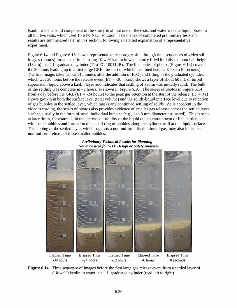
6.30
Kaolin was the solid component of the slurry in all but one of the tests, and water was the liquid phase in
all but two tests, which used 10 wt% NaCl solution. The matrix of completed preliminary tests and
results are summarized later in this section, following a detailed explanation of a representative
experiment.
Figure 6.14 and Figure 6.15 show a representative test progression through time sequences of video still
images (photos) for an experiment using 10 wt% kaolin in water slurry filled initially to about half height
(18 cm) in a 1 L graduated cylinder (Test FG 100114B). The first series of photos (Figure 6.14) covers
the 30 hours leading up to a first large GRE, the start of which is defined here as ET zero (0 seconds).
The first image, taken about 14 minutes after the addition of H2O2 and filling of the graduated cylinder,
which was 30 hours before the release event (ET = -30 hours), shows a layer of about 60 mL of turbid
supernatant liquid above a kaolin layer and indicates that settling of kaolin was initially rapid. The bulk
of the settling was complete in ~2 hours, as shown in Figure 6.16. The series of photos in Figure 6.14
from a day before the GRE (ET = -24 hours) to the peak gas retention at the start of the release (ET = 0 s)
shows growth in both the surface level (total volume) and the solids-liquid interface level due to retention
of gas bubbles in the settled layer, which masks any continued settling of solids. As is apparent in the
video recording, the series of photos also provides evidence of smaller gas releases across the settled layer
surface, usually in the form of small individual bubbles (e.g., 1 to 3 mm diameter estimated). This is seen
at later times, for example, in the increased turbidity of the liquid due to entrainment of fine particulate
with some bubbles and formation of a small ring of bubbles along the cylinder wall at the liquid surface.
The sloping of the settled layer, which suggests a non-uniform distribution of gas, may also indicate a
non-uniform release of these smaller bubbles.
Preliminary Technical Results for Planning –
Not to be used for WTP Design or Safety Analyses
Elapsed Time
-30 hours
Elapsed Time
-24 hours
Elapsed Time
-12 hours
Elapsed Time
-6 hours
Elapsed Time
0 seconds
Figure 6.14. Time sequence of images before the first large gas release event from a settled layer of
(10-wt%) kaolin in water in a 1 L graduated cylinder (read left to right)
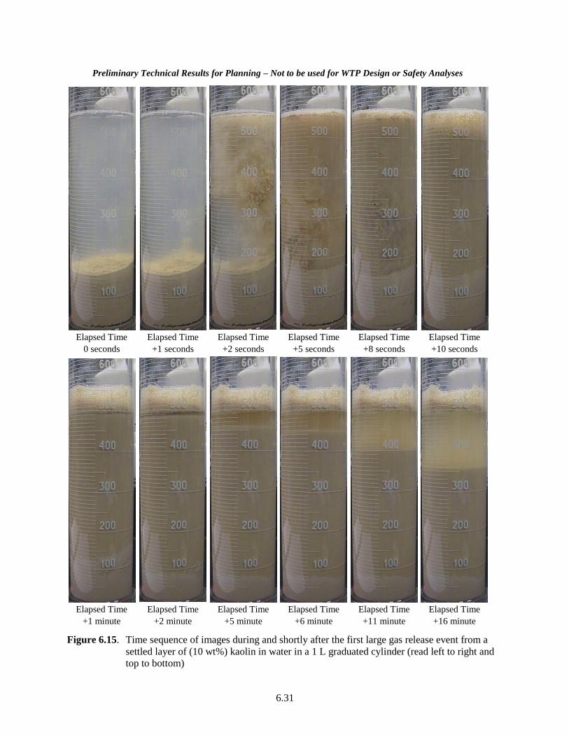
6.31
Preliminary Technical Results for Planning – Not to be used for WTP Design or Safety Analyses
Elapsed Time
0 seconds
Elapsed Time
+1 seconds
Elapsed Time
+2 seconds
Elapsed Time
+5 seconds
Elapsed Time
+8 seconds
Elapsed Time
+10 seconds
Elapsed Time
+1 minute
Elapsed Time
+2 minute
Elapsed Time
+5 minute
Elapsed Time
+6 minute
Elapsed Time
+11 minute
Elapsed Time
+16 minute
Figure 6.15. Time sequence of images during and shortly after the first large gas release event from a
settled layer of (10 wt%) kaolin in water in a 1 L graduated cylinder (read left to right and
top to bottom)
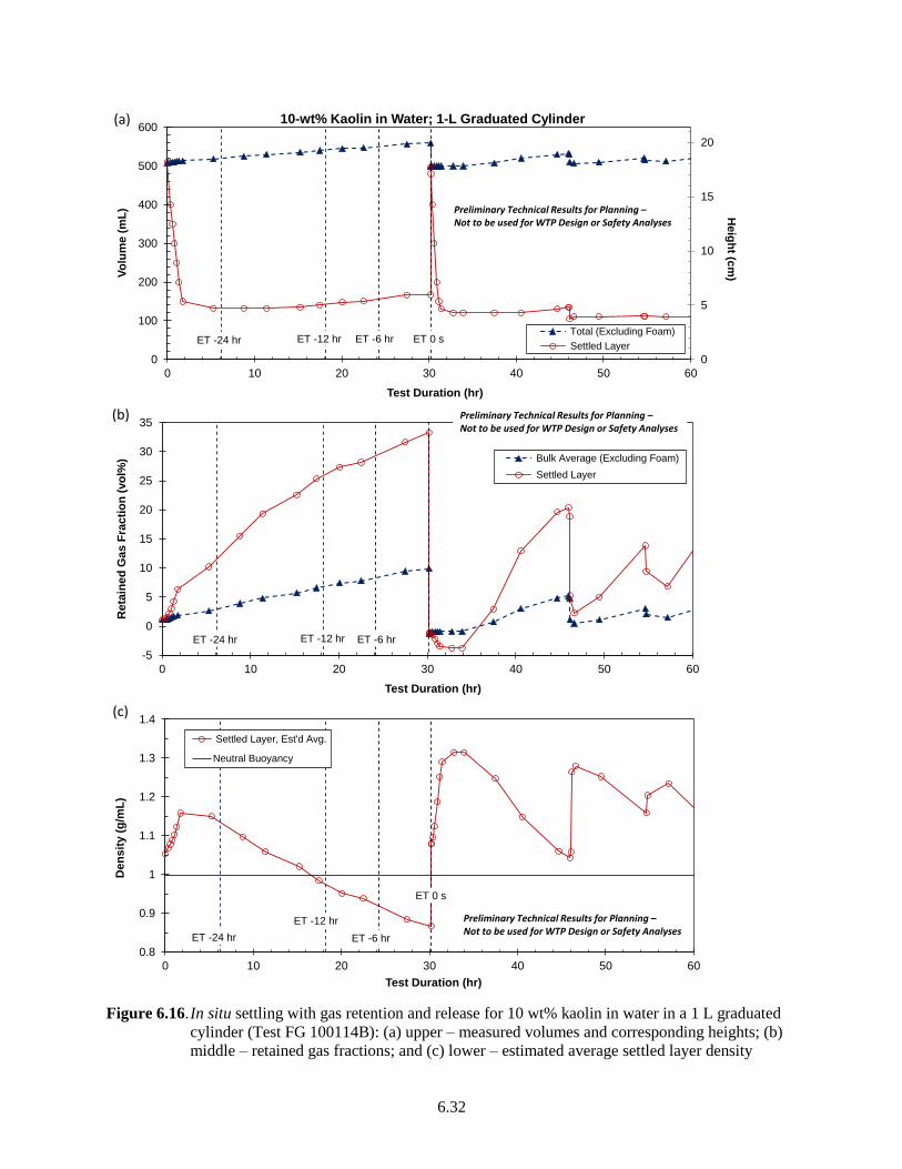
6.32
Figure 6.16. In situ settling with gas retention and release for 10 wt% kaolin in water in a 1 L graduated
cylinder (Test FG 100114B): (a) upper – measured volumes and corresponding heights; (b)
middle – retained gas fractions; and (c) lower – estimated average settled layer density
ET 0 sET -6 hrET -12 hrET -24 hr
0
5
10
15
20
0
100
200
300
400
500
600
0 10 20 30 40 50 60
He
igh
t (cm
)Vo
lum
e (
mL
)
Test Duration (hr)
10-wt% Kaolin in Water; 1-L Graduated Cylinder
Total (Excluding Foam)
Settled Layer
Preliminary Technical Results for Planning –Not to be used for WTP Design or Safety Analyses
(a)
ET -6 hrET -12 hrET -24 hr
-5
0
5
10
15
20
25
30
35
0 10 20 30 40 50 60
Reta
ine
d G
as
Fra
cti
on
(vo
l%)
Test Duration (hr)
Bulk Average (Excluding Foam)
Settled Layer
Preliminary Technical Results for Planning –Not to be used for WTP Design or Safety Analyses
(b)
ET 0 s
ET -6 hr
ET -12 hr
ET -24 hr
0.8
0.9
1
1.1
1.2
1.3
1.4
0 10 20 30 40 50 60
Den
sit
y (
g/m
L)
Test Duration (hr)
Settled Layer, Est'd Avg.
Neutral Buoyancy
Preliminary Technical Results for Planning –Not to be used for WTP Design or Safety Analyses
(c)

6.33
The upper series of photos in Figure 6.15 shows the large gas release event, which was substantially
complete in 10 seconds, and the lower sequence of images shows partial re-settling in the first 16 minutes
after the GRE. At ET = +1 second, a few bubbles are visible in the water, emanating from the upper-half
of the settled layer. In the few seconds following, a plume of solids is visible in the liquid, first starting in
the path of the initial bubbles and then fully encompassing the settled layer (e.g., images at ET = +2 and
+5 seconds). While release of some individual bubbles can be seen (more readily in the video), the
release event is overall characterized as a buoyant displacement (i.e., BDGRE), because the initial
retained gas fraction exceeded that for the settled layer to be neutrally buoyant in the water and, in part,
due to the visual information. For example, in addition to the obvious plume of solids, there are some
small floating “gobs” of gaseous solids visible in the darker near-surface areas of the photos at ET = +5
and +8 seconds. The extent of the engagement of the settled layer in the GRE is hidden by a residual
“coating” of solids along the wall, which still appears to be ≥150 mL at ET = +10 seconds and >~120 mL
at ET = +1 minute. However, sloughing of solids from the wall and filling of the core is evident in the
decrease in volume of this band of residual solids to ≤80 mL at ET = +5 to +16 minutes.
The extent of the release is also blurred by the foam / froth layer on top. The presence of a substantial
layer of foam (>50 mL) becomes more apparent at ET = +10 seconds and is readily seen at ET = +1
minute in the developing liquid layer between ~490 and 500 mL. Although not thought to be
quantitatively significant in terms of the mass (and gas-free volume) of solids and water held up in the
foam, the foam distorts the liquid surface and makes reading the total volume (minus foam) difficult.
Both factors contribute to apparent, but unrealistic, negative gas fractions in the period following the large
GRE.
Derived from still images such as those shown in Figure 6.14 and Figure 6.15, Figure 6.16 shows
quantitative results over the course of 2.5 days of the ~3 day test. The upper plot shows the surface level
and the estimated solids-liquid interface level in terms of directly measured volumes (the raw data) and
the corresponding heights calculated from a measured height/volume factor. Vertical lines in the plots
indicate elapsed time relative to the first large GRE and correspond to photos in Figure 6.14. The y-axis
in Figure 6.16 represents a vertical line at essentially ET = -30 hours, for comparison to the sequence of
photos, and no additional vertical line was added for this point in time. The middle plot shows the
calculated retained gas fractions in the bulk slurry volume (αB) and the estimated average in the settled
layer (αsl). The overall αB is the retained gas volume, Vg, divided by the measured total volume, Vtotal,
where Vg is the change in volume from the initial gas-free volume1 (Vg = Vtotal - Vinit). The average gas
fraction in the settled layer, where all the gas is retained, is Vg divided by the gaseous settled layer
volume, Vsl. The latter, more so than Vtotal, is an approximate value because of non-uniformity in the
surface level of the settled layer as shown in Figure 6.14, for example. This and previously noted
challenges in reading the total volume after the large GRE due to foam (Figure 6.15) contribute to
irregular, negative gas fraction data in Figure 6.16 at 30+ hours into the test (ET > 0 seconds).
The lower plot of Figure 6.16 shows the variation of estimated average density of the settled layer during
the test in comparison to the density at neutral buoyancy (e.g., the density of water). Neglecting the mass
of retained gas, the gaseous settled layer density, ρsl, is approximated as the sum of masses of solids (msol)
and liquid in the layer (mL,sl) divided by the volume of the layer:
𝜌𝑠𝑙 =
𝑚𝑠𝑜𝑙 + 𝑚𝐿,𝑠𝑙
𝑉𝑠𝑙
=𝑚𝑠𝑜𝑙 + (𝑉𝑠𝑙 − 𝑉𝑠𝑜𝑙 − 𝑉𝑔) 𝜌𝐿⁄
𝑉𝑠𝑙
=𝑚𝑠𝑜𝑙 + (𝑉𝑠𝑙 −
𝑚𝑠𝑜𝑙𝜌𝑠𝑜𝑙
⁄ − 𝑉𝑔) 𝜌𝐿⁄
𝑉𝑠𝑙
6.1
1 The initial gas-free volume was calculated from the mass of slurry added and the theoretical slurry density
(Eq. 5.12 in Section 5.5.2.2).

6.34
where the volume of solids, Vsol, is written in terms of the mass-averaged density of solids, ρsol, in the
right-hand form of the equation. It was assumed that all solids in the vessel were in the settled (or
settling) layer, and msol in Eq. 6.1 is the product of the mass of slurry added to the vessel and the solids
mass fraction xS. At the time of the large release event in Figure 6.16, ρsl was 0.87 g/mL and the settled
layer was super-buoyant relative to the supernatant water (gas fraction greater than neutral buoyancy).
While there was likely a gradient in the retained gas, solid, and liquid fractions in the settled layer, the
low average density supports the conclusion drawn from the visual data that gas was released in a
BDRGE.
The behavior after the large BDGRE depicted in Figure 6.16 is representative of most other settling with
gas retention and release tests that were conducted. These characteristics include multiple cycles of
settling, retention, and release in which: a) the settled layer often reached higher density than the initial
cycle (e.g., up to 1.31 g/mL in the test shown); the minimum densities were higher and the peak gas
fractions were lower before secondary releases; and secondary gas releases were often smaller and/or less
complete. Secondary releases in some tests may have been BDGREs even if the average ρsl was greater
than ρL. This could occur, for example, if a fraction of the gaseous settled layer was not involved in a first
GRE and it continued to retain gas and became buoyant in a subsequent release event. If not BDGREs,
larger primary and secondary gas releases typically exhibited characteristics of bubble cascades
(Section 6.1).
Test conditions and results of the preliminary settling with gas retention and release experiments in 1 L
graduated cylinders and 10 in. and 23 in. diameter vessels are summarized in Table 6.3 (these results are
also compared to model predictions in Figure 7.16). The Bingham rheology of pre-H2O2 slurry was
measured on samples from a number of the tests, and the results are tabulated in Appendix D.1 Kaolin
was the exclusive solid component used in the tests except for a 1 L graduated cylinder experiment with
10 wt% 90:10 M30:B in water simulant (Test FG 111414A). After two initial 1 L cylinder
“demonstration” tests using 20 wt% kaolin in water (Tests FG 092414A and FG 092414B), the
subsequent tests used solids contents of either 5 wt% or 10 wt%. In higher density liquid such as the
10 wt% NaCl solution used in two 1 L cylinder tests (Tests FG 101314A and FG 101314B), the volume
fraction of solids at a given weight fraction is slightly higher than in lower density liquid (e.g.,
≤10 percent more solids by volume in the NaCl solution than in water). The primary results shown in
Table 6.3 are the estimated peak retained gas fractions in the bulk slurry and in the settled layer
immediately preceding the first large GREs. The gas fractions in these events were typically, but not
always, larger than for secondary release events. The table also shows the initial gas-free bulk slurry
density, the liquid density, and the minimum settled layer density at the GRE estimated using Eq. 6.1.
Comparison of the latter two provides an indication whether the gas release was a BDGRE or by some
other spontaneous release mechanism such as BC. In all but a few of the tests, ρsl was within 0.01 g/mL
of, or less than, ρL suggesting that BD was the predominant release mechanism. In Section 7.2, bulk
average gas fraction data in Table 6.3 are compared to model predictions for peak gas retention associated
with BDGREs from settling beds of solids in low-solids vessels.
Two tests, in which settling and/or gas release behavior were different, clearly did not exhibit global
BDGREs in the first spontaneous GREs. One of these was the 1 L cylinder test using 10 wt%
90:10 M30:B slurry in water (ρsl = 1.08 g/mL at the GRE). Overall, the solids did not appear to settle as
readily as kaolin and the gas generation rate seemed considerably faster. The latter was perhaps due to
the bentonite content (see Section 5.5.3.3), even though the H2O2 concentration in the test (0.16 M) was
1 Bingham parameters are provided in Table D.1 of Appendix D for pre-H2O2 addition samples from the following
tests shown in Table 6.3: FG 092414A, FG 092414A, 23-05, 23-08, FG 101314A, and FG 101314B. Note that the
solids contents of the pre-H2O2 rheology samples were higher than used in their respective settling tests, and,
therefore, the tabulated results only provide upper bounds on the Bingham yield stress and consistency.
6.35
approximately half that in most of the kaolin tests (0.29 M). The nearly immediate and continuous stream
of round bubbles and smaller particle sizes of the solids compared to kaolin both likely contributed to
diminished settling and a very murky “liquid” phase. This made visual characterization of the larger
release event difficult. The GRE appeared to initiate with, and was primarily defined by, the release of a
relatively large bubble (e.g., ~1 cm); however it could not be determined if an associated BC or a
localized BD occurred. Smaller round bubbles (e.g., roughly 1 to 2 mm) continued to be retained in
settled material toward the bottom of the vessel, suggesting that the release event was restricted to
(possibly) less-densely packed and weaker material above. The 10 wt% kaolin in water test in the 10 in.
vessel was also atypical (Test FG 10-12; ρsl = 1.12 g/mL at the GRE), which is suspected to be due to
addition of small amounts of 2 M HCl to the liquid phase to reduce pH to 3-4. This was done in an
attempt to enhance flocculation of the kaolin and improve clarity of the liquid phase to improve
observations of gas release behavior. The effects of NaCl concentration and pH on the settling behavior
of kaolin in water are discussed, for example, in Nasser and James (2006). The reduced pH may have
impacted flocculation and the structure of the settled bed, but improvement in visibility was not sufficient
(if any) to see the liquid-settled layer interface during the GRE. The effect of the pH adjustment on the
gas generation rate in the test was indeterminate, although it was expected to be lower (Section 5.5.3.3).
However, the elapsed time after filling the vessel to the first GRE was <7 hours, compared to ~30 hours
for the 10 wt% kaolin in water graduated cylinder test shown in Figure 6.16. This is consistent with the
GRE occurring at a lower retained gas fraction and higher average settled layer density in Test FG 10-12.
These data highlight the need for additional testing to better understand the roles of settling and gas
generation rates and settled layer structure on gas release behavior.
Although no attempt has been made here to draw conclusions about the effect of initial slurry depth or fill
H/D ratio, these data are included in Table 6.3 for reference. The table also shows the molar
concentration of H2O2 in the liquid phase. It was held constant (0.29 M) in all but the 90:10 M30:B test
discussed above and one of the initial pair of tests using 20 wt% kaolin, from which the target
concentration was selected for most other preliminary tests. Again, the data are too limited to provide
insight into the possible effects of gas generation rate.
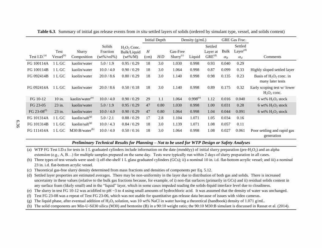
6.3
6
Table 6.3. Summary of initial gas release events from in situ settled layers of solids (ordered by simulant type, vessel, and solids content)
Test I.D.(a)
Test
Vessel(b)
Slurry
Composition
Solids
Fraction
(wt%/vol%)
H2O2 Conc.
Bulk/Liquid
(wt%/M)
Initial Depth Density (g/mL) GRE Gas Frac.
Comments
H
(cm) H/D
Gas-Free
Slurry(c)
Liquid
Settled
Layer at
GRE(d)
Bulk
B
Settled
Layer(d)
sl
FG 100114A 1 L GC kaolin/water 5.0 / 1.9 0.95 / 0.29 18 3.0 1.030 0.998 0.93 0.040 0.29
FG 100114B 1 L GC kaolin/water 10.0 / 4.0 0.90 / 0.29 18 3.0 1.064 0.998 0.87 0.099 0.33 Highly sloped settled layer
FG 092414B 1 L GC kaolin/water 20.0 / 8.6 0.80 / 0.29 18 3.0 1.140 0.998 0.98 0.135 0.23 Basis of H2O2 conc. in
many later tests
FG 092414A 1 L GC kaolin/water 20.0 / 8.6 0.50 / 0.18 18 3.0 1.140 0.998 0.89 0.175 0.32 Early scoping test w/ lower
H2O2 conc.
FG 10-12 10 in. kaolin/water(e)
10.0 / 4.0 0.90 / 0.29 29 1.1 1.064 0.998(e)
1.12 0.016 0.040 6 wt% H2O2 stock
FG 23-05 23 in. kaolin/water 5.0 / 1.9 0.95 / 0.29 47 0.80 1.030 0.998 1.00 0.031 0.28 6 wt% H2O2 stock
FG 23-08(f)
23 in. kaolin/water 10.0 / 4.0 0.90 / 0.29 47 0.80 1.064 0.998 1.04 0.044 0.091 6 wt% H2O2 stock
FG 101314A 1 L GC kaolin/salt(g)
5.0 / 2.1 0.88 / 0.29 17 2.8 1.104 1.071 1.05 0.034 0.16
FG 101314B 1 L GC kaolin/salt(g)
10.0 / 4.3 0.84 / 0.29 18 3.0 1.139 1.071 1.08 0.057 0.11
FG 111414A 1 L GC M30:B/water(h)
10.0 / 4.0 0.50 / 0.16 18 3.0 1.064 0.998 1.08 0.027 0.061 Poor settling and rapid gas
generation
Preliminary Technical Results for Planning – Not to be used for WTP Design or Safety Analyses
(a) WTP FG Test I.D.s for tests in 1 L graduated cylinders include information on the date (mmddyy) of initial slurry preparation (pre-H2O2) and an alpha
extension (e.g., A, B…) for multiple samples prepared on the same day. Tests were typically run within 2 days of slurry preparation in all cases.
(b) Three types of test vessels were used: i) off-the-shelf 1 L glass graduated cylinders (GCs); ii) a nominal 10 in. i.d. flat-bottom acrylic vessel; and iii) a nominal
23 in. i.d. flat-bottom acrylic vessel.
(c) Theoretical gas-free slurry density determined from mass fractions and densities of components per Eq. 5.12.
(d) Settled layer properties are estimated averages. There may be non-uniformity in the layer due to distribution of both gas and solids. There is increased
uncertainty in these values (relative to the bulk gas fractions because, for example, of i) non-flat surfaces (primarily in GCs) and ii) residual solids content in
any surface foam (likely small) and in the “liquid” layer, which in some cases impeded reading the solids-liquid interface level due to cloudiness.
(e) The slurry in test FG 10-12 was acidified to pH ~3 to 4 using small amounts of hydrochloric acid. It was assumed that the density of water was unchanged.
(f) Test FG 23-08 was a repeat of Test FG 23-06, which was not usable for quantitative gas release data because of issues with video cameras.
(g) The liquid phase, after eventual addition of H2O2 solution, was 10 wt% NaCl in water having a theoretical (handbook) density of 1.071 g/mL.
(h) The solid components are Min-U-Sil30 silica (M30) and bentonite (B) in a 90:10 weight ratio; the 90:10 M30:B simulant is discussed in Rassat et al. (2014).
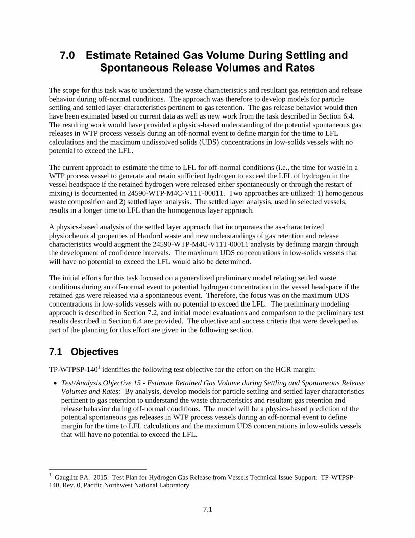
7.1
7.0 Estimate Retained Gas Volume During Settling and Spontaneous Release Volumes and Rates
The scope for this task was to understand the waste characteristics and resultant gas retention and release
behavior during off-normal conditions. The approach was therefore to develop models for particle
settling and settled layer characteristics pertinent to gas retention. The gas release behavior would then
have been estimated based on current data as well as new work from the task described in Section 6.4.
The resulting work would have provided a physics-based understanding of the potential spontaneous gas
releases in WTP process vessels during an off-normal event to define margin for the time to LFL
calculations and the maximum undissolved solids (UDS) concentrations in low-solids vessels with no
potential to exceed the LFL.
The current approach to estimate the time to LFL for off-normal conditions (i.e., the time for waste in a
WTP process vessel to generate and retain sufficient hydrogen to exceed the LFL of hydrogen in the
vessel headspace if the retained hydrogen were released either spontaneously or through the restart of
mixing) is documented in 24590-WTP-M4C-V11T-00011. Two approaches are utilized: 1) homogenous
waste composition and 2) settled layer analysis. The settled layer analysis, used in selected vessels,
results in a longer time to LFL than the homogenous layer approach.
A physics-based analysis of the settled layer approach that incorporates the as-characterized
physiochemical properties of Hanford waste and new understandings of gas retention and release
characteristics would augment the 24590-WTP-M4C-V11T-00011 analysis by defining margin through
the development of confidence intervals. The maximum UDS concentrations in low-solids vessels that
will have no potential to exceed the LFL would also be determined.
The initial efforts for this task focused on a generalized preliminary model relating settled waste
conditions during an off-normal event to potential hydrogen concentration in the vessel headspace if the
retained gas were released via a spontaneous event. Therefore, the focus was on the maximum UDS
concentrations in low-solids vessels with no potential to exceed the LFL. The preliminary modeling
approach is described in Section 7.2, and initial model evaluations and comparison to the preliminary test
results described in Section 6.4 are provided. The objective and success criteria that were developed as
part of the planning for this effort are given in the following section.
7.1 Objectives
TP-WTPSP-1401 identifies the following test objective for the effort on the HGR margin:
Test/Analysis Objective 15 - Estimate Retained Gas Volume during Settling and Spontaneous Release
Volumes and Rates: By analysis, develop models for particle settling and settled layer characteristics
pertinent to gas retention to understand the waste characteristics and resultant gas retention and
release behavior during off-normal conditions. The model will be a physics-based prediction of the
potential spontaneous gas releases in WTP process vessels during an off-normal event to define
margin for the time to LFL calculations and the maximum UDS concentrations in low-solids vessels
that will have no potential to exceed the LFL.
1 Gauglitz PA. 2015. Test Plan for Hydrogen Gas Release from Vessels Technical Issue Support. TP-WTPSP-
140, Rev. 0, Pacific Northwest National Laboratory.
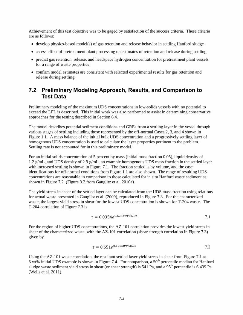
7.2
Achievement of this test objective was to be gaged by satisfaction of the success criteria. These criteria
are as follows:
develop physics-based model(s) of gas retention and release behavior in settling Hanford sludge
assess effect of pretreatment plant processing on estimates of retention and release during settling
predict gas retention, release, and headspace hydrogen concentration for pretreatment plant vessels
for a range of waste properties
confirm model estimates are consistent with selected experimental results for gas retention and
release during settling.
7.2 Preliminary Modeling Approach, Results, and Comparison to Test Data
Preliminary modeling of the maximum UDS concentrations in low-solids vessels with no potential to
exceed the LFL is described. This initial work was also performed to assist in determining conservative
approaches for the testing described in Section 6.4.
The model describes potential sediment conditions and GREs from a settling layer in the vessel through
various stages of settling including those represented by the off-normal Cases 2, 3, and 4 shown in
Figure 1.1. A mass balance of the initial bulk UDS concentration and a progressively settling layer of
homogenous UDS concentration is used to calculate the layer properties pertinent to the problem.
Settling rate is not accounted for in this preliminary model.
For an initial solids concentration of 5 percent by mass (initial mass fraction 0.05), liquid density of
1.2 g/mL, and UDS density of 2.9 g/mL, an example homogenous UDS mass fraction in the settled layer
with increased settling is shown in Figure 7.1. The fraction settled is by volume, and the case
identifications for off-normal conditions from Figure 1.1 are also shown. The range of resulting UDS
concentrations are reasonable in comparison to those calculated for in situ Hanford waste sediment as
shown in Figure 7.2 (Figure 3.2 from Gauglitz et al. 2010a).
The yield stress in shear of the settled layer can be calculated from the UDS mass fraction using relations
for actual waste presented in Gauglitz et al. (2009), reproduced in Figure 7.3. For the characterized
waste, the largest yield stress in shear for the lowest UDS concentration is shown for T-204 waste. The
T-204 correlation of Figure 7.3 is
𝜏 = 0.0354𝑒0.6233𝑤𝑡%𝑈𝐷𝑆 7.1
For the region of higher UDS concentrations, the AZ-101 correlation provides the lowest yield stress in
shear of the characterized waste, with the AZ-101 correlation (shear strength correlation in Figure 7.3)
given by
𝜏 = 0.651𝑒0.1756𝑤𝑡%𝑈𝐷𝑆 7.2
Using the AZ-101 waste correlation, the resultant settled layer yield stress in shear from Figure 7.1 at
5 wt% initial UDS example is shown in Figure 7.4. For comparison, a 50th percentile median for Hanford
sludge waste sediment yield stress in shear (or shear strength) is 541 Pa, and a 95th percentile is 6,439 Pa
(Wells et al. 2011).
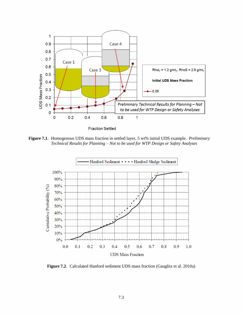
7.3
Figure 7.1. Homogenous UDS mass fraction in settled layer, 5 wt% initial UDS example. Preliminary
Technical Results for Planning – Not to be used for WTP Design or Safety Analyses
Figure 7.2. Calculated Hanford sediment UDS mass fraction (Gauglitz et al. 2010a)

7.4
Figure 7.3. Slurry yield stress in shear as a function of UDS mass fraction (Wt.% UDS) (Gauglitz et al.
2009)
Figure 7.4. Yield stress in shear of settled layer, 5 wt% initial UDS example. Preliminary Technical
Results for Planning – Not to be used for WTP Design or Safety Analyses
7.5
For Figure 7.4, the settled layer condition at a given fraction settled is independent of prior conditions;
thus, as previously specified, settling and compaction rates are not accounted for, nor is the effect of
developing rheology on that settling. In addition, the potential increase of the yield stress in shear with
time, at a specific UDS fraction, is also not addressed (e.g., Wells et al. 2011). A discussion of the
preliminary development of settling and rheological models to address these behaviors is provided in
Appendix F.
The retention of generated gas in a time-varying settled solids layer is dependent on many different
physicochemical processes including the rate of settling, the rate of aggregation, compaction and the
settled layer rheology with time. These processes are typically coupled with each other and, more
importantly, dependent on the underlying physiochemical properties of the waste. In addition to
neglecting the effects of time on the settled layer condition for the preliminary modeling, the gas
generation rate and resultant accumulation are also not modeled for this initial evaluation. With these
assumptions, two conditions are represented for the gas fraction that may be retained within the settled
layer with respect to spontaneous gas releases. First, approximating the BDGRE spontaneous gas releases
described in Section 4.2, the gas volume fraction is limited by neutral buoyancy. Neutral buoyancy, NB,
can be expressed with the supernatant liquid layer density, L, and the settled layer density ρ as
𝛼𝑁𝐵 = 1 −𝜌𝐿
𝜌
7.3
In actuality, the gas fraction required for a BDGRE is likely greater than neutral buoyancy as the buoyant
material must overcome the strength of the surrounding material or attachment to vessel floor and walls,
as described in Section 4.0. Meyer et al. (1997), which defined this increased gas fraction as the critical
gas fraction, developed an expression relating the upward force due to buoyancy and the restraining force
due to the yield stress in the material. That expression is not employed in this preliminary modeling as
there are limited data to establish the applicability of the relation to the waste conditions of interest.
However, Eq. 7.3 may under-represent the retained gas fraction at which a BDGRE may occur.
The second modeled gas fraction limit represents BC spontaneous releases (see Section 6.1) and is taken
from a curve representing the bentonite clay data of Gauglitz et al. (1996) shown in Table 6.1. This
maximum gas fraction as a function of waste strength (yield stress in shear) is shown in Figure 7.5, which
is reproduced from Rassat et al. (1998). Also included in the figure are actual laboratory waste gas
fraction measurements and a pictorial characterization of the retained gas bubble morphology (i.e., the
blue shapes at the bottom of the figure). For reference, the slit, or crack, shapes depicted for ~ 1,000 Pa
are the focus of the conclusions of Meacham et al. (2014), which argues that the BDGRE phenomena
does not occur for wastes with sufficiently high shear strength.
The neutral buoyant gas fraction and maximum gas fraction (representation of Figure 7.5 dashed line) for
the 5 wt% UDS example are shown in Figure 7.6. For the conditions with a smaller fraction settled, the
maximum gas fraction is less than the neutral buoyant gas fraction. Physically this implies that a BC will
occur prior to a BDGRE. As the fraction settled increases, the relation switches, so BDRGEs are
indicated to occur prior to sufficient gas fraction for a BC to occur. This behavior is depicted in
Figure 7.7 where the two curves with different symbol and color distinguish the mechanism that should
occur. At the example conditions, BCs occur up to 20 percent by volume, with BDGREs occurring
subsequently.
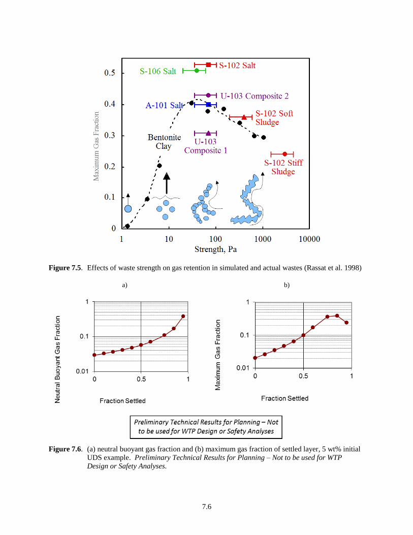
7.6
Figure 7.5. Effects of waste strength on gas retention in simulated and actual wastes (Rassat et al. 1998)
a)
b)
Figure 7.6. (a) neutral buoyant gas fraction and (b) maximum gas fraction of settled layer, 5 wt% initial
UDS example. Preliminary Technical Results for Planning – Not to be used for WTP
Design or Safety Analyses.
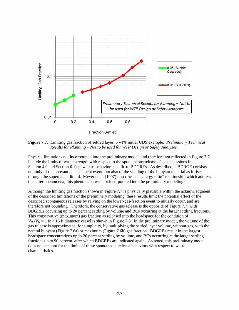
7.7
Figure 7.7. Limiting gas fraction of settled layer, 5 wt% initial UDS example. Preliminary Technical
Results for Planning – Not to be used for WTP Design or Safety Analyses.
Physical limitations not incorporated into the preliminary model, and therefore not reflected in Figure 7.7,
include the limits of waste strength with respect to the spontaneous releases (see discussions in
Section 4.0 and Section 6.1) as well as behavior specific to BDGREs. As described, a BDRGE consists
not only of the buoyant displacement event, but also of the yielding of the buoyant material as it rises
through the supernatant liquid. Meyer et al. (1997) describes an “energy ratio” relationship which address
the latter phenomena; this phenomena was not incorporated into the preliminary modeling.
Although the limiting gas fraction shown in Figure 7.7 is physically plausible within the acknowledgment
of the described limitations of the preliminary modeling, these results limit the potential effect of the
described spontaneous releases by relying on the lower-gas-fraction event to initially occur, and are
therefore not bounding. Therefore, the conservative gas release is the opposite of Figure 7.7, with
BDGREs occurring up to 20 percent settling by volume and BCs occurring at the larger settling fractions.
This conservative (maximum) gas fraction as released into the headspace for the condition of
VHS/VW = 1 in a 16 ft diameter vessel is shown in Figure 7.8. In the preliminary model, the volume of the
gas release is approximated, for simplicity, by multiplying the settled layer volume, without gas, with the
neutral buoyant (Figure 7.6a) or maximum (Figure 7.6b) gas fraction. BDGREs result in the largest
headspace concentrations up to 20 percent settling by volume, and BCs occurring at the larger settling
fractions up to 90 percent, after which BDGREs are indicated again. As noted, this preliminary model
does not account for the limits of these spontaneous release behaviors with respect to waste
characteristics.
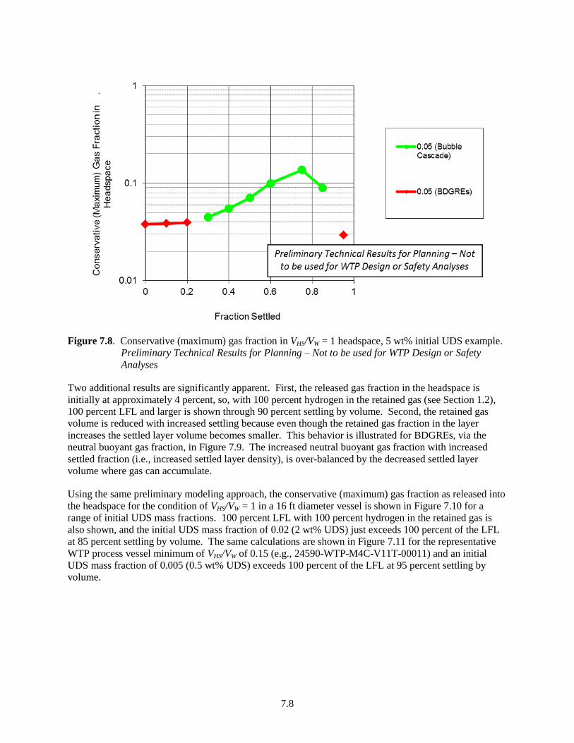
7.8
Figure 7.8. Conservative (maximum) gas fraction in VHS/VW = 1 headspace, 5 wt% initial UDS example.
Preliminary Technical Results for Planning – Not to be used for WTP Design or Safety
Analyses
Two additional results are significantly apparent. First, the released gas fraction in the headspace is
initially at approximately 4 percent, so, with 100 percent hydrogen in the retained gas (see Section 1.2),
100 percent LFL and larger is shown through 90 percent settling by volume. Second, the retained gas
volume is reduced with increased settling because even though the retained gas fraction in the layer
increases the settled layer volume becomes smaller. This behavior is illustrated for BDGREs, via the
neutral buoyant gas fraction, in Figure 7.9. The increased neutral buoyant gas fraction with increased
settled fraction (i.e., increased settled layer density), is over-balanced by the decreased settled layer
volume where gas can accumulate.
Using the same preliminary modeling approach, the conservative (maximum) gas fraction as released into
the headspace for the condition of VHS/VW = 1 in a 16 ft diameter vessel is shown in Figure 7.10 for a
range of initial UDS mass fractions. 100 percent LFL with 100 percent hydrogen in the retained gas is
also shown, and the initial UDS mass fraction of 0.02 (2 wt% UDS) just exceeds 100 percent of the LFL
at 85 percent settling by volume. The same calculations are shown in Figure 7.11 for the representative
WTP process vessel minimum of VHS/VW of 0.15 (e.g., 24590-WTP-M4C-V11T-00011) and an initial
UDS mass fraction of 0.005 (0.5 wt% UDS) exceeds 100 percent of the LFL at 95 percent settling by
volume.
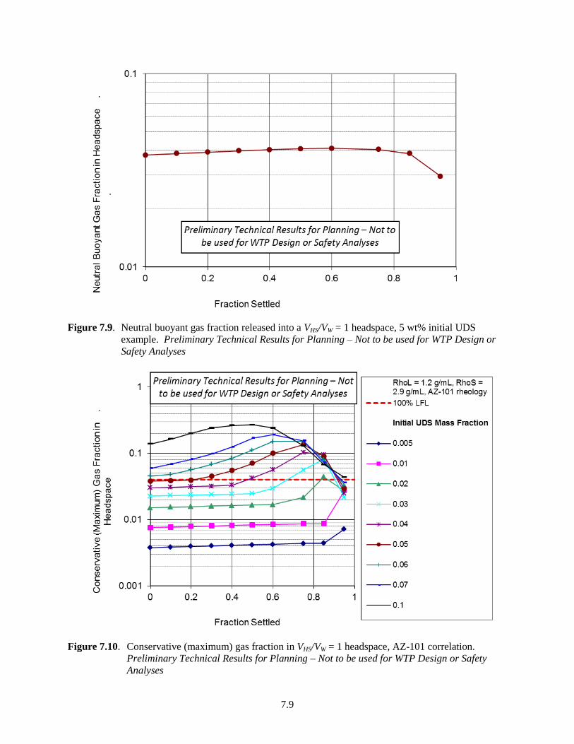
7.9
Figure 7.9. Neutral buoyant gas fraction released into a VHS/VW = 1 headspace, 5 wt% initial UDS
example. Preliminary Technical Results for Planning – Not to be used for WTP Design or
Safety Analyses
Figure 7.10. Conservative (maximum) gas fraction in VHS/VW = 1 headspace, AZ-101 correlation.
Preliminary Technical Results for Planning – Not to be used for WTP Design or Safety
Analyses

7.10
Figure 7.11. Conservative (maximum) gas fraction in VHS/VW = 0.15 headspace, AZ-101 correlation.
Preliminary Technical Results for Planning – Not to be used for WTP Design or Safety
Analyses
As described, the preliminary model does not account for the limits of the spontaneous release behaviors
with respect to waste characteristics. However, both the 2 wt% and 0.5 wt% initial UDS settled layers at
the fraction settled that resulted in 100 percent LFL for spontaneous releases both have yield stress in
shear values that are plausible, based on the AZ-101 correlation (Eq. 7.2). Figure 7.12 shows the yield
stress in shear estimates for these settling layers.
The effect of the waste rheology correlation is shown in Figure 7.13, which uses the T-204 correlation
(Eq. 7.1) at equal liquid and solid densities to those used for the AZ-101 modeling. Increased yield stress
in shear values result, and the implications to the conservative (maximum) gas fraction as released into
the headspace for the conditions of VHS/VW = 1 and VHS/VW = 0.15 in a 16 ft diameter vessel are shown in
Figure 7.14 and Figure 7.15, respectively. As for the AZ-101 correlation, gas release from the 2 wt% and
0.5 wt% UDS settled layers exceed 100 percent LFL, so UDS concentrations less than these values would
be needed to avoid the potential of exceeding 100 percent LFL. Again, these layers have yield stress in
shear values calculated for the T-204 correlation (Eq. 7.1) that are quite plausible for the represented
spontaneous release mechanisms.
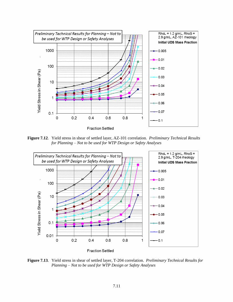
7.11
Figure 7.12. Yield stress in shear of settled layer, AZ-101 correlation. Preliminary Technical Results
for Planning – Not to be used for WTP Design or Safety Analyses
Figure 7.13. Yield stress in shear of settled layer, T-204 correlation. Preliminary Technical Results for
Planning – Not to be used for WTP Design or Safety Analyses
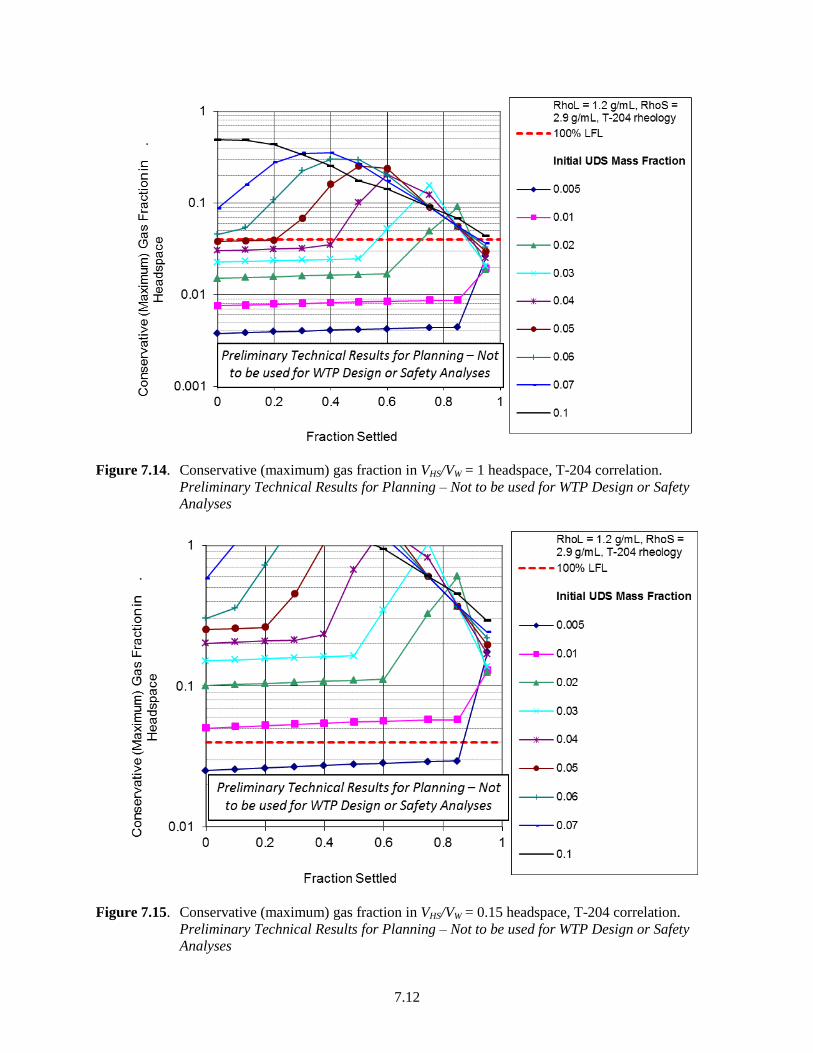
7.12
Figure 7.14. Conservative (maximum) gas fraction in VHS/VW = 1 headspace, T-204 correlation.
Preliminary Technical Results for Planning – Not to be used for WTP Design or Safety
Analyses
Figure 7.15. Conservative (maximum) gas fraction in VHS/VW = 0.15 headspace, T-204 correlation.
Preliminary Technical Results for Planning – Not to be used for WTP Design or Safety
Analyses
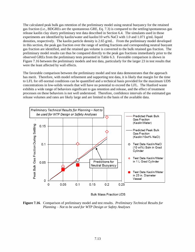
7.13
The calculated peak bulk gas retention of the preliminary model using neutral buoyancy for the retained
gas fraction (i.e., BDGREs are the spontaneous GRE, Eq. 7.3) is compared to the settling/spontaneous gas
release kaolin clay slurry preliminary test data described in Section 6.4. The simulants used in those
experiments are identified by kaolin/water and kaolin/10 wt% NaCl with 1.0 and 1.071 g/mL liquid
densities, respectively. The kaolin particle density is 2.65 g/mL. From the preliminary model developed
in this section, the peak gas fraction over the range of settling fractions and corresponding neutral buoyant
gas fraction are identified, and the retained gas volume is converted to the bulk retained gas fraction. The
preliminary model results can thus be compared directly to the peak gas fractions immediately prior to the
observed GREs from the preliminary tests presented in Table 6.3. Favorable comparison is shown in
Figure 7.16 between the preliminary models and test data, particularly for the larger 23 in test results that
were the least affected by wall effects.
The favorable comparison between the preliminary model and test data demonstrates that the approach
has merit. Therefore, with model refinement and supporting test data, it is likely that margin for the time
to LFL for off-normal conditions can be quantified and a technical basis provided for the maximum UDS
concentrations in low-solids vessels that will have no potential to exceed the LFL. The Hanford waste
exhibits a wide range of behaviors significant to gas retention and release, and the effect of treatment
processes on these behaviors is not well understood. Therefore, confidence intervals of the estimated gas
release volumes and rates are likely large and are limited to the basis of the available data.
Figure 7.16. Comparison of preliminary model and test results. Preliminary Technical Results for
Planning – Not to be used for WTP Design or Safety Analyses

8.1
8.0 Assess Margin in Hydrogen Generation Rate Estimates
The HGR model used in WTP studies has been shown (Sherwood and Stock 2004) to provide a
conservative margin for most tank wastes against which it has been tested, and additional margin is
contributed by conservatism in many of the inputs used in safety studies. However, in-process conditions
and postulated conditions during loss-of-power events can include higher temperatures, greater dilution,
higher solids fractions, and/or higher hydroxide concentrations than were present in the tank waste
samples used in HGR testing.
In addition, the reactivity of organics, a major source of hydrogen in many parts of the WTP process, has
been defined for relatively few tank wastes. This unknown quantity of hydrogen could lead to
overestimation or underestimation of the HGR for some waste streams, with resulting effects on the
calculation of the time to the LFL.
In addition, the existing correlations for HGR by organics include coefficients that depend implicitly on
the typical range of concentrations of nitrite and hydroxide that are found in the unprocessed high-salt
tank wastes on which HGR testing was largely conducted. However, dissolved ion concentrations can
change rate controlling steps and turn on or off reactions that convert total organic carbon (TOC) to
hydrogen. Nitrite and hydroxide concentrations must be sufficiently high to allow the
aluminate-catalyzed thermolytic conversion of organics to hydrogen, and in “organic radiolysis” high
hydroxide concentrations are necessary to produce hydrogen from intermediates such as formaldehyde
and glyoxylate. Other largely-unassessed effects are those of “background” HGR (that which may exist
in the absence of radioactivity, oxygen, and aluminate), of loss of decay energy to non-reactive fractions
of the waste, and of radiolysis of water of hydration in precipitated solids.
8.1 Objectives
TP-WTPSP-1401 identifies the following test objective for the effort on the HGR margin:
Test/Analysis Objective 13 – Margin in Hydrogen Generation Rate Estimates: By analysis, assess the
conservatism of HGR mechanisms that are currently included in the HGR model, using existing HGR
test results and outside literature. Expand the understanding of the effect of differences between the
conditions on which model development was based (the “training-set” of data) and conditions in the
plant, using existing HGR test results and outside literature. Identify vessels in which doses and
concentrations of hydroxide, nitrite, aluminate, and TOC are significantly different from those present
in samples used for HGR model development, by using the WTP flowsheet and possibly data from
the PEP tests to track the unit HGR throughout the pretreatment process.
Achievement of this test objective was to be gaged by satisfaction of the success criteria. These criteria
are as follows:
evaluate how much margin in HGR is present for the “worst” batches in a feed vector, for WTP
process conditions representing vessels whose HGR behavior is important to hydrogen safety
compare these to the HGRs calculated to obtain time-to-LFL for the same points in the process.
1 Gauglitz PA. 2015. Test Plan for Hydrogen Gas Release from Vessels Technical Issue Support. TP-WTPSP-
140, Rev. 0, Pacific Northwest National Laboratory.

8.2
8.2 Technical Approach and Progress
The planned approach was to use existing HGR test results and outside literature, to assess the HGR
mechanisms currently included in the HGR model, and to expand the understanding of the effect of
differences between the conditions on which model development was based (the “training-set” of data)
and conditions in the PTF. The task scope also included using data from the PEP tests and the WTP
flowsheet to track the unit HGR throughout the pretreatment process and identify vessels and piping in
which concentrations of hydroxide, nitrite, aluminate, and TOC would be significantly different from
those present in samples used for HGR model development. The conservatism in the flowsheet
assumptions was to be evaluated in terms of how much margin was added at different conditions.
At the time of project shutdown, this task had not progressed far enough to allow any reportable
conclusions; the status of the various planned, or partly completed, activities was as follows:
Assessment of the uncertainty in the feed vector. This activity was to consider 1) uncertainty in the
source information (i.e., the Best Basis Inventory), 2) uncertainty in the solubility models in the
Hanford Task Waste Operations Simulator (HTWOS) model used to model blending and dilution of
waste streams, and 3) uncertainty arising from lack of uniformity of solids concentration and
composition during retrieval from each tank. Some information was gathered, but no analysis had
begun.
Assessment of the margin added (or lost) due to time-to-LFL analysis assumptions about process
conditions. Some documents describing the time-to-LFL analyses and their sources were obtained
and reviewed, but no analysis had begun.
Assessment of the margin in the WTP HGR correlation (Sherwood and Stock 2004). The status of
this subtask is detailed below in terms of the following individual activities:
– Assessment of HGR correlation margin related to TOC reactivity. This activity had not begun.
Its scope included estimating the contribution of oxalate (which is non-reactive) to the total
dissolved TOC concentration that is used as a model input and testing the HGR model against
existing data for simulants in which different species were used to represent TOC.
– Assessment of HGR correlation margin related to hydroxide concentrations above or below those
used in HGR model development. This activity had not begun.
– Assessment of HGR correlation margin related to nitrite concentrations above or below those
used in HGR model development. This activity had not begun.
– Assessment of the effect of the water fraction of liquid on the water radiolysis part of the HGR
correlation. Data were collected and calculations were initiated but not completed.
– Assessment of whether radiolysis HGR was different for water of hydration in the solid phase
than for water in liquid. This activity had not begun.
– Assessment of whether mechanisms exist that could produce significant hydrogen in the absence
of radiation and organics. This activity had not begun.
– Assessment of margin added or lost because of the combination of process conditions and
different reactivity behaviors of waste. Because the HGR correlation is a combination of
correlations for different hydrogen-producing mechanisms, different mechanisms dominate in
different parts of the process. Because each individual waste may have a different response to
dose and temperature (for organic radiolysis) and to temperature (for organic thermolysis), and
these differences may not be describable by a single reactivity factor and standardized activation
energies as used in the WTP HGR, there might be a combination of some waste and some process
condition that lies outside the expected envelope around the HGR correlation’s predictions. The

8.3
planned approach was to make HGR predictions using a set of newly generated HGR correlation
models for six well-characterized single wastes (i.e., 241-AW-101, SY-103, A-101, S-102, S-106,
and U-103). These models, and the WTP HGR correlation, were to be exercised with the same
process streams given in Attachment H of Eager et al. (2006) or other existing process stream
information. This task had begun. Preliminary single-waste HGR correlations had been
developed at the time the project was shut down, but needed conceptual review and were not
ready for reporting.
– Assessment of the margin added or lost owing to assumptions made about process conditions in
evaluating the HGR and the time to LFL. This activity had begun but did not proceed far enough
to be reported.
Appendix M of Eager et al. (2006) provided a study that discussed the following categories of operating
margins:
Mass balance associated margins. These margins included feed Na molarity and solids content used
in a “normal” mass-balance run (using the same sources for solids and liquids composition),
throughput rate, accumulation of anti-foaming agent, and dissolved resin.
Time to LFL calculation associated margins. These margins included waste volume and headspace
volume, temperature, volume occupied by solids in the waste, partial release of hydrogen, and more
frequent mixing.
WTP HGR correlation associated margins. These margins included the concentrations of soluble
TOC and Al, the presence of dissolved carbon in the form of non-reactive oxalate versus reactive
organic compounds, and the effect of low-reactivity organics including anti-foaming agents and
normal paraffin hydrocarbons.
The mass-balance and time-to-LFL margins were quantified by Appendix M of Eager et al. (2006).
However, a 2010 Engineering Calculation Change Notice (ECCN) (Eager 2010a) replaced the HGRs and
times to LFL and the associated calculations in Eager et al. (2006) with those in a revised set of
calculations (Eager 2010b). Appendix M of Eager et al. (2006) was not revised or updated to match the
new information in Eager (2010b).
Eager et al. (2006) currently is the document that presents and stores the approved inputs and assumptions
that support the hydrogen calculations in Eager (2010b), which as of 2010 is the approved source of
results. However, in some cases, inputs and assumptions have been changed between Eager et al. (2006)
and Eager (2010b). Table 8.1 provides a summary of the more significant changes. Some of these are
assumptions that would be worth including in a new margins analysis. Assumptions related to the settled
solids layer may be particularly significant.

8.4
Table 8.1. Assumptions related to HGR and time-to-LFL calculations in original and revised documents
Assumption/Input
Eager et al. (2006)
24590-WTP-M4C-V11T-00004
Rev. C
Eager (2010b)
24590-WTP-M4C-V11T-00011
Rev. C
Design feed composition LAW liquid: AP-103, 10 M Na
LAW solid: AY-102, 3.8 wt%
HLW liquid: AP-103, 10 M Na
HLW solid: AY-102, 200 g/L.
Source is TFCOUP 5A
Same, but the basis date for decay was
changed from 1/1/2011 to 1/1/2018.
Specific activities and
decay energies
Defined in Table 2-2 of Eager et al.
(2006). 10% is added to the heat
load to cover isotopes that are not
specifically included.
Same.
Waste volume Maximum volume: either overflow
or high-high alarm minus internals
displacement. Solids are assumed to
occupy no volume, so liquid volume
= slurry volume.
Some of the vessels where no settled layer is
assumed have a deduction for volume of
internals. Some, but not all, tanks have
changes in waste or headspace volume.
Settled layer None; all vessels are modeled with
uniformly mixed slurry
In some vessels with Newtonian slurries,
settling is assumed, producing a clear liquid
layer overlying a settled solids layer
containing 76 vol% liquid. Only the gas
generated within the solids layer is retained.
Headspace volume Half or all the high mixing volume
(depending on vessel) is credited as
headspace.
Similar; also, 1% of headspace volume is
subtracted to account for internals.
Temperature Either maximum operating
temperature or post-DBE
temperature, whichever is higher.
Vessels where no settled layer is assumed
use the maximum operating temperature. In
settled layers, temperatures are modeled over
time, based on heat-transfer assumptions
starting from the maximum operating
temperature.
Composition changes
due to processing
Mass-balance spreadsheet
calculations are used.
Same.
LFL The H2 LFL is 4 vol% at 25°C, 3.01
vol% at 100°C, and linear in-
between. The effect of flammable
gases other than H2 is negligible.
Same.
Starting H2
concentration
0.5% H2 for vessels with Newtonian
slurry, approximately zero for others.
0.5% H2 for vessels with settled layers; for
others, total HGR divided by minimum
purge air.
HGR correlation Sherwood and Stock (2004). Same.
LAW = low-activity waste; HLW = high-level waste; THCOUP 5A = the feed vector in revision 5A of the Tank
Farm Contractor’s Operation and Utilization Plan.
9.1
9.0 Elevated H2 Concentration Due to Plumes
Plumes of flammable gas may be produced by releases of retained gas over essentially the entire waste
area (“global”) or over a small fraction of the area (“local”). Past estimates of deflagration consequences
from global and local plumes in Hanford waste tanks have shown that the estimated pressure rises from
plume deflagrations do not endanger tank integrity. However, calculations in these studies have generally
been based on pure hydrogen releases, in which the high flammability of the release is, to some extent,
offset by enhanced mixing caused by high buoyancy. Actual releases are likely to include both buoyant
species (e.g., hydrogen) and denser-than-air species (e.g., nitrous oxide). In addition, the aspect ratio
(height or diameter) of a WTP vessel headspace may differ from that on which existing estimates were
based.
9.1 Objectives
TP-WTPSP-1401 identifies the following test objective for the effort on the HGR margin:
Test/Analysis Objective 14 – Elevated H2 Concentration Due to Plumes: By analysis, review past
plume hazard studies (Epstein and Burelbach 1998a, 1998b) for applicability in WTP process vessels,
and calculate consequences for buoyant plumes, focusing primarily on the transient global model that
estimates maximum flammable volume and duration of flammable conditions. Use existing data
from actual releases (in waste tanks or in large test systems) to estimate possible gas release rates.
Where possible, existing studies in the literature will be used to qualitatively discuss the possible
effects on mixing of aspect-ratio variation or heavier-than-air gases.
Achievement of this test objective was to be gaged by satisfaction of the success criteria. These criteria
are as follows:
provide parametric evaluations of the maximum flammable volume (or mass) and duration for a
representative set of WTP vessels, release rates, and release-gas compositions
calculate peak pressure from deflagration.
9.2 Technical Approach
The planned approach for addressing the hazard from plumes was to review past plume hazard studies
(Epstein and Burelbach 1998a; 1998b) for applicability in WTP process vessels and calculate
consequences for buoyant plumes, focusing primarily on the transient global model (Epstein and
Burelbach 1998a) that estimates maximum flammable volume and duration of flammable conditions. The
approach was to use existing data from actual releases (in waste tanks or in large test systems) to estimate
possible gas release rates. Where possible, studies in the literature were to be used to qualitatively discuss
the possible effects of aspect-ratio variation or heavier-than-air gases on mixing in vessel headspaces.
The two models of plumes in headspaces developed for Hanford waste tank studies are discussed in
Section 9.3 and Section 9.4. Section 9.5 summarizes questions about the models’ assumptions. The main
scenario-related inputs to the plume models, which are discussed in Section 9.6, are the superficial release
velocity of the gas at the surface of the waste and the gas properties of density and LFL. The input-
related effort at the close-out of this task included assessments of the gas release velocity and the gas
1 Gauglitz PA. 2015. Test Plan for Hydrogen Gas Release from Vessels Technical Issue Support. TP-WTPSP-
140, Rev. 0, Pacific Northwest National Laboratory.
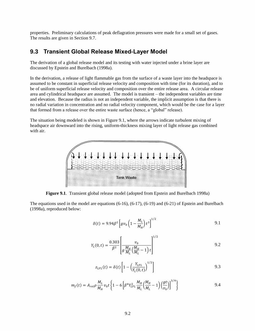
9.2
properties. Preliminary calculations of peak deflagration pressures were made for a small set of gases.
The results are given in Section 9.7.
9.3 Transient Global Release Mixed-Layer Model
The derivation of a global release model and its testing with water injected under a brine layer are
discussed by Epstein and Burelbach (1998a).
In the derivation, a release of light flammable gas from the surface of a waste layer into the headspace is
assumed to be constant in superficial release velocity and composition with time (for its duration), and to
be of uniform superficial release velocity and composition over the entire release area. A circular release
area and cylindrical headspace are assumed. The model is transient – the independent variables are time
and elevation. Because the radius is not an independent variable, the implicit assumption is that there is
no radial variation in concentration and no radial velocity component, which would be the case for a layer
that formed from a release over the entire waste surface (hence, a “global” release).
The situation being modeled is shown in Figure 9.1, where the arrows indicate turbulent mixing of
headspace air downward into the rising, uniform-thickness mixing layer of light release gas combined
with air.
Figure 9.1. Transient global release model (adopted from Epstein and Burelbach 1998a)
The equations used in the model are equations (6-16), (6-17), (6-19) and (6-21) of Epstein and Burelbach
(1998a), reproduced below:
𝛿(𝑡) = 9.94𝛽2 [𝑔𝑣0 (1 −
𝑀𝐿
𝑀𝐻
) 𝑡3]1 2⁄
9.1
𝑌𝐿(0, 𝑡) =0.303
𝛽2[
𝑣0
𝑔𝑀𝐻
𝑀𝐿(
𝑀𝐻
𝑀𝐿− 1) 𝑡
]
1 2⁄
9.2
𝑧𝐿𝐹𝐿(𝑡) = 𝛿(𝑡) [1 − (
𝑌𝐿𝐹𝐿
𝑌𝐿(0, 𝑡))
1 2⁄
] 9.3
𝑚𝑓(𝑡) = 𝐴𝑟𝑒𝑙𝜌
𝑀𝐿
𝑀𝐻
𝑣0𝑡 {1 − 6 [𝛽4𝑌𝐿𝐹𝐿2
𝑀𝐻
𝑀𝐿
(𝑀𝐻
𝑀𝐿
− 1) (𝑔𝑡
𝑣0
)]3 4⁄
} 9.4
9.3
where 𝛿(𝑡) = mixing layer thickness
𝑌𝐿(0, 𝑡) = mass fraction of light gas at the bottom (z = 0) of the mixing layer
𝑚𝑓(𝑡) = mass of light (flammable) gas in the flammable zone of the layer, the part where
concentration is greater than the LFL
t = time
= empirical mixing-length-thickness proportionality coefficient (relates turbulent mixing
length to mixing layer thickness)
𝑣0 = vertical superficial release velocity of light gas
g = acceleration of gravity
MH = molecular weight of the heavy gas (headspace air)
ML = molecular weight of the light (flammable) gas
= density of the air/light-gas mixture; because the Boussinesq approximation is used in
the derivation, this can consistently be taken to equal the density of headspace air, H.
YLFL = mass fraction of the light gas at its LFL
Arel = area of surface over which light gas is released
zLFL = thickness of the flammable zone (height above waste surface)
Note that the height of the headspace, H, is not an input to the model. The aspect ratio of the headspace is
also not an input. From the point of view of the model formulation, the only impact of H is that at the
time the mixing layer reaches the top of the headspace the model becomes invalid because the upper
boundary condition in the model derivation (zero light-gas concentration) is no longer true, and after that
time the peak flammable mass cannot be predicted using these equations.
The scenario-related inputs to the model are the release velocity, the gas composition, in terms of density
and LFL, and the release area. Further quantities of interest were also derived by Epstein and Burelbach
(1998a), including the maximum flammable gas mass (𝑚𝑓,𝑚𝑎𝑥), the release time at which the maximum
occurs (tmax), the thickness of the flammable zone at tmax (zLFL,max), the duration of the flammable zone’s
existence (tlife), and the time at which the top of the mixing layer reaches the top of the headspace (tD).
The average light-gas concentration in the flammable zone can be calculated and compared to the bulk
flammable-gas concentration in the headspace that would exist at the time of the peak flammable mass, if
the whole headspace were completely mixed. The comparison suggests what fraction of the bulk
well-mixed LFL would provide a safe criterion to govern maximum allowable releases. The range of
average flammable-zone concentrations and flammable-zone thicknesses during the duration of
flammability also may be of interest in terms of evaluating the probability of detonation.
The overpressure consequences of deflagration in an (assumed) unvented vessel can be estimated with
Eq. (6-27) (mislabeled as [6-25] in the reference) from Epstein and Burelbach (1998a):
𝑃
𝑃0
= [1 + (𝜌𝑢
𝜌𝑏
− 1)𝑉𝑓,𝑚𝑖𝑥
𝑉]
𝛾𝑏
9.5
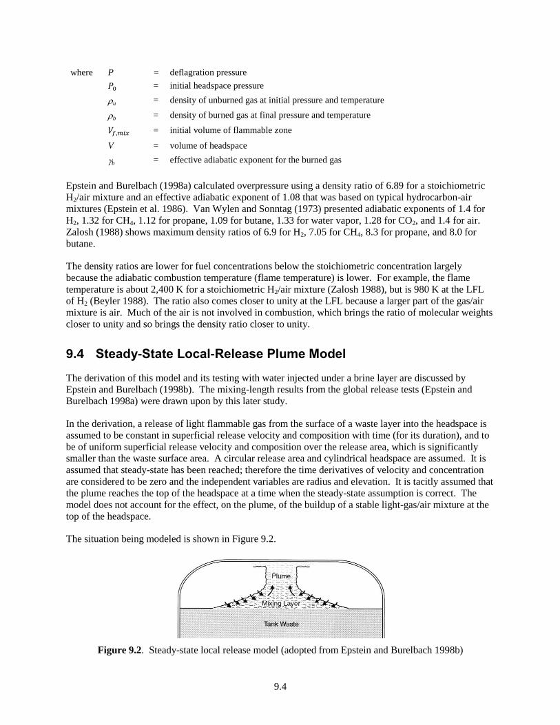
9.4
where P = deflagration pressure
𝑃0 = initial headspace pressure
u = density of unburned gas at initial pressure and temperature
b = density of burned gas at final pressure and temperature
𝑉𝑓,𝑚𝑖𝑥 = initial volume of flammable zone
V = volume of headspace
b = effective adiabatic exponent for the burned gas
Epstein and Burelbach (1998a) calculated overpressure using a density ratio of 6.89 for a stoichiometric
H2/air mixture and an effective adiabatic exponent of 1.08 that was based on typical hydrocarbon-air
mixtures (Epstein et al. 1986). Van Wylen and Sonntag (1973) presented adiabatic exponents of 1.4 for
H2, 1.32 for CH4, 1.12 for propane, 1.09 for butane, 1.33 for water vapor, 1.28 for CO2, and 1.4 for air.
Zalosh (1988) shows maximum density ratios of 6.9 for H2, 7.05 for CH4, 8.3 for propane, and 8.0 for
butane.
The density ratios are lower for fuel concentrations below the stoichiometric concentration largely
because the adiabatic combustion temperature (flame temperature) is lower. For example, the flame
temperature is about 2,400 K for a stoichiometric H2/air mixture (Zalosh 1988), but is 980 K at the LFL
of H2 (Beyler 1988). The ratio also comes closer to unity at the LFL because a larger part of the gas/air
mixture is air. Much of the air is not involved in combustion, which brings the ratio of molecular weights
closer to unity and so brings the density ratio closer to unity.
9.4 Steady-State Local-Release Plume Model
The derivation of this model and its testing with water injected under a brine layer are discussed by
Epstein and Burelbach (1998b). The mixing-length results from the global release tests (Epstein and
Burelbach 1998a) were drawn upon by this later study.
In the derivation, a release of light flammable gas from the surface of a waste layer into the headspace is
assumed to be constant in superficial release velocity and composition with time (for its duration), and to
be of uniform superficial release velocity and composition over the release area, which is significantly
smaller than the waste surface area. A circular release area and cylindrical headspace are assumed. It is
assumed that steady-state has been reached; therefore the time derivatives of velocity and concentration
are considered to be zero and the independent variables are radius and elevation. It is tacitly assumed that
the plume reaches the top of the headspace at a time when the steady-state assumption is correct. The
model does not account for the effect, on the plume, of the buildup of a stable light-gas/air mixture at the
top of the headspace.
The situation being modeled is shown in Figure 9.2.
Figure 9.2. Steady-state local release model (adopted from Epstein and Burelbach 1998b)

9.5
For a known gas composition, release velocity, and release area, the model predicts the following
steady-state quantities:
the radial profile of vertically uniform (assumed) concentration in the mixing layer
the radial profile of the mixing layer thickness
the concentration at the base of the plume
the dimensions of the mixing layer and plume
the vertical profile of radially uniform (assumed) concentration in the plume
the concentration in the plume at the elevation of the top of the headspace.
The model, as presented by Epstein and Burelbach, focused on finding the flammable-gas concentration
at the top of the headspace. It does not include equations for flammable gas mass. It would be possible to
carry out further derivation to calculate (at steady-state) the total mass of flammable gas in the layer and
plume, the mass of flammable gas in the flammable zone of the layer and plume, the height to which the
flammable zone reaches in the plume, and the earliest time at which steady-state would be reached (total
mass of flammable gas divided by the assumed-constant release rate). However, these derivations have
not yet been performed.
The steady-state local release model does not allow tracking flammable-gas concentration over time, to
find the time and quantity of the maximum flammable mass during release and the dimensions of the
plume and layer at the time of maximum flammable mass. Nor does it allow determination of the
duration of flammability. A transient local plume model would have to be derived to provide those types
of predictions, and this was not in the scope of the task.
9.5 Questions About the Model Assumptions
A literature review was to be conducted to evaluate the effect of conditions not considered in the transient
global and steady-state local release models. This effort is currently incomplete, but the pertinent
conditions are discussed in the remainder of this section.
9.5.1 Headspace Aspect Ratio
In the Epstein and Burelbach (1998a; 1998b) models, the dilution and expansion of the released light gas
is produced by buoyancy-driven turbulent mixing. Because the diffusion coefficient of turbulent mixing
depends more on larger eddies than on smaller ones, and because the maximum eddy size is limited by
the minimum dimension of the headspace, the aspect ratio of the headspace might be expected to affect
the mixing length of the layer of released gas. It is consistent with this expectation that Epstein and
Burelbach (1998a) commented that in the tall narrow “headspace” in a vertical tube, with a high aspect
ratio, other experimenters had found that the turbulent mixing length was proportional to the tube
diameter, which was the limiting dimension.
The brine/water tests that supported the Epstein and Burelbach models had an effective “headspace”
(upper brine layer) aspect ratio of about 0.9. In the conceptual design of the SHSVD, the headspace
aspect ratio is about 0.8 when the vessel is filled to a depth where the headspace volume equals the waste
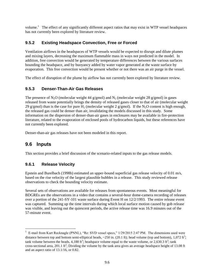
9.6
volume.1 The effect of any significantly different aspect ratios that may exist in WTP vessel headspaces
has not currently been explored by literature review.
9.5.2 Existing Headspace Convection, Free or Forced
Ventilation airflows in the headspaces of WTP vessels would be expected to disrupt and dilute plumes
and mixing layers, decreasing the maximum flammable mass in ways not predicted in the model. In
addition, free convection would be generated by temperature differences between the various surfaces
bounding the headspace, and by buoyancy added by water vapor generated at the waste surface by
evaporation. This free convection would be present whether or not there was an air purge in the vessel.
The effect of disruption of the plume by airflow has not currently been explored by literature review.
9.5.3 Denser-Than-Air Gas Releases
The presence of N2O (molecular weight 44 g/gmol) and N2 (molecular weight 28 g/gmol) in gases
released from waste potentially brings the density of released gases closer to that of air (molecular weight
29 g/gmol) than is the case for pure H2 (molecular weight 2 g/gmol). If the N2O content is high enough,
the released gas could be denser than air, invalidating the models discussed in this study. Some
information on the dispersion of denser-than-air gases in enclosures may be available in fire-protection
literature, related to the evaporation of enclosed pools of hydrocarbon liquids, but these references have
not currently been explored.
Denser-than-air gas releases have not been modeled in this report.
9.6 Inputs
This section provides a brief discussion of the scenario-related inputs to the gas release models.
9.6.1 Release Velocity
Epstein and Burelbach (1998b) estimated an upper-bound superficial gas release velocity of 0.01 m/s,
based on the rise velocity of the largest plausible bubbles in a release. This study reviewed release
observations to check the bounding velocity estimate.
Several sets of observations are available for releases from spontaneous events. Most meaningful for
BDGREs are the observations in a video that contains a several-hour dome-camera recording of releases
over a portion of the 241-SY-101 waste surface during Event H on 12/2/1993. The entire release event
was captured. Summing up the time intervals during which local surface motion caused by gob release
was visible, and leaving out the quiescent periods, the active release time was 16.9 minutes out of the
57-minute event.
1 E-mail from Kurt Recknagle (PNNL), “Re: SVD vessel specs,” 1/29/2015 2:47 PM. The dimensions used were
distance between top and bottom semi-elliptical heads, ~250 in. (20.1 ft); head volume (top and bottom), 1,072 ft3;
tank volume between the heads, 4,188 ft3; headspace volume equal to the waste volume, or 2,630.3 ft
3; tank
cross-sectional area, 201.1 ft2; Dividing the volume by the tank area gives an average headspace height of 13.08 ft
and an aspect ratio of 13.1/16, or 0.82.

9.7
According to Johnson et al. (2000), the event released 7,000 ft3 of gas (at 1 atm) out of an estimated
inventory of 11,400 ft3 (at in situ pressure). Factoring the in situ hydrostatic pressure into the inventory,
approximately 25 to 33 percent of the inventory was released by Event H.
The average superficial release velocity, based on the total waste surface area of 410 m2 and the release
volume and active duration, can be calculated at 0.00048 m/s. However, the release area probably did not
involve the whole waste surface. Because it is difficult to judge the release area from the video, it is
assumed that the release area was approximately 25 percent of the surface, roughly consistent with the
fraction of inventory released. Under this assumption, the superficial release velocity during active
release periods in Event H in SY-101 was 0.0019 m/s.
Event H produced a peak headspace H2 concentration of 27,400 ppm (Johnson et al. 2000). Other
BDGREs on 12/4/1991 and 9/3/1992 produced peak concentrations about twice as high as that from
Event H, though the released gas volumes were only 10 to 30 percent higher. These events probably had
higher overall release rates. The releases may have been less interrupted in these events, or the superficial
release velocity may have been greater, or both. Assuming that all of the increases in release rate came
from velocity, the release velocity in the higher-H2 events might have been as high as 0.004 m/s.
Spontaneous GREs in other DSTs provide further information. Wells et al. (2002) describes a number of
events in tanks AN-103, AN-104, AN-105, and AW-101, providing a tabulation of the release volumes
and the release time constants for each released gob of buoyant waste, as estimated from data for
headspace ventilation, H2 concentration versus time, and volume, as well as H2 fraction in the gas.
The gobs with the highest release volumes and high ratios of volume per time constant (high release rates)
were selected for analysis in this study; these gob releases were typically associated with the largest
headspace H2 peaks. The selected parameters were used to calculate volumetric release rates, which
ranged from 0.001 to 0.014 m3/s. Because these release rates are for single gobs, they do not need to be
adjusted for interruptions in the release. The fraction of inventory released by these single gobs ranged
from approximately 1 to 23 percent of the inventory. The estimate of fractional release is approximate,
because the inventories used in calculations were those measured by retained gas sampling (Mahoney et
al. 1999), not the inventories at the time of release.
When the release is taken to have been over the entire waste surface area, the highest superficial release
velocity in these events is calculated to be 0.000035 m/s, from a gob in the 5/30/1996 release in
241-AN-105. The fraction of inventory released was about 18 percent. If the fraction of surface area
involved in this release is taken to have been equal to the fraction of inventory released, the superficial
release velocity over the limited release area would be 0.00019 m/s. The highest superficial release
velocity over the limited release area was 0.0009 m/s, which occurred in the 2/1/1999 event in
241-AN-103. Here the estimated release fraction was 0.6 percent of the inventory.
Note that this set of DSTs did not have any estimated superficial release velocity as high as that in
SY-101, nor were the peak headspace H2 concentrations as high. Of the set of gobs considered, the one
that produced the highest peak headspace H2 concentration was the AN-105 gob discussed previously.
Superficial release velocities were also estimated from data for releases of O2 gas generated and retained
in layers of clay simulant in 70 in. diameter test vessels (Rassat et al. 2014). The data included videos of
the entire release events, total clay surface areas, start and end times for releases, and release volumes. It
was possible to visually estimate the fraction of the surface area involved in the releases. The releases
were uninterrupted.
9.8
Tests 70-26, 70-28, 70-30, and 70-20 (Rassat et al. 2014) were selected for analysis because of their high
release fractions: respectively, 80, 91, 67, and 57 percent of the gas inventory. Of these tests, 70-26,
70-28, and 70-30 used conditions where gas was generated throughout a single simulant layer with a
minimal thickness of supernatant liquid. The gas release mechanism was considered to be a BC in these
tests, in which most of the gas was released in 2 to 6 minutes. In test 70-20, gas was generated in the
lower part of the simulant, which was overlaid by a layer of the same simulant in which there was no gas
and by a thin layer of supernatant. This test showed a RT gas release mechanism, with lower-layer solids
(identified by the dye color) being ejected together with gas. In this test, the duration of the release of
most of the gas was 4 minutes. The superficial release velocities were calculated conservatively by
assuming all of the observed gas release occurred during the period of most rapid release. The BC release
velocities over the release areas in the single-layer tests ranged from 0.0007 to 0.004 m/s, while the
velocity was 0.0031 m/s for the RT event in the double-layer test. These velocities are comparable to or
higher than the ones calculated for BDGREs in DSTs.
Finally, an additional release-rate datum is provided by a BC event that fortuitously occurred in a 34 in.
vessel that had been set up with clay simulant for PJM testing (see Section 6.1.4.2). Essentially all of the
17 vol% retained O2 gas in the waste was released in 15 seconds, producing an estimated superficial
velocity of about 0.009 m/s, the highest observed release velocity. Note, however, that this event
occurred in the smallest vessel of any discussed here. The more rapid release velocity may be a function
of the smaller vessel size.
The observations reviewed are consistent with the argument made by Epstein and Burelbach (1998b) that
a superficial release velocity of 0.01 m/s would be a bounding value.
9.6.2 Release-Gas Properties
The release-gas properties of concern are the release gas LFL and the ratio of the release gas density to
that of air. Assuming that the temperature and pressure of the release gas are the same as the those of the
headspace air, which is an approximation, the ratio of densities is equal to the ratio of molecular weights
(as assumed by Epstein and Burelbach 1998a, 1998b). The LFLs of gas mixtures were calculated from
the component LFLs at 25°C using LeChatelier’s linear mixing law (Mahoney et al. 2000). The gases
ethane, propane, and n-butane were taken to be representatives for C2Hx, C3Hx, and other hydrocarbons.
Three different release-gas compositions were considered: pure H2, the composition measured in SY-101
mixed slurry at riser 23A by retained gas sampling (Mahoney et al. 1999), and the gas produced during
HGR testing of self-irradiated oxygenated AN-106 liquid at 90°C (Sherwood and Stock 2004). The gases
were chosen to include a range of density and flammability that would answer the question of whether
higher flammability and lower density (faster dispersion of the plume) produced a greater risk than lower
flammability and higher density (slower dispersion of the plume).
Table 9.1 shows the properties of these gases. The gases are given on an NH3-free, CO2-free basis, on the
assumption that although these soluble species might be generated, they would be captured by liquid
under post-design-basis conditions in WTP vessels, rather than being promptly released.
The LFLs for hydrocarbons other than methane were taken from Beyler (1988): 0.030 mole fraction for
ethane, 0.021 mole fraction for propane, and 0.018 mole fraction for n-butane. Sherwood and Stock
(2004) did not break out non-methane hydrocarbons (NMHC) by number of carbons, so the original data
supplied by Bryan et al. (2004) were drawn upon to assign NMHC species.
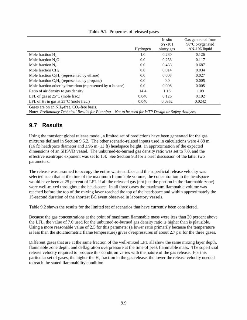
9.9
Table 9.1. Properties of released gases
Hydrogen
In situ
SY-101
slurry gas
Gas generated from
90°C oxygenated
AN-106 liquid
Mole fraction H2 1.0 0.280 0.126
Mole fraction N2O 0.0 0.258 0.117
Mole fraction N2 0.0 0.433 0.687
Mole fraction CH4 0.0 0.014 0.034
Mole fraction C2Hx (represented by ethane) 0.0 0.008 0.027
Mole fraction C3Hx (represented by propane) 0.0 0.0 0.005
Mole fraction other hydrocarbon (represented by n-butane) 0.0 0.008 0.005
Ratio of air density to gas density 14.4 1.15 1.09
LFL of gas at 25°C (mole frac.) 0.040 0.126 0.192
LFL of H2 in gas at 25°C (mole frac.) 0.040 0.0352 0.0242
Gases are on an NH3-free, CO2-free basis.
Note: Preliminary Technical Results for Planning – Not to be used for WTP Design or Safety Analyses
9.7 Results
Using the transient global release model, a limited set of predictions have been generated for the gas
mixtures defined in Section 9.6.2. The other scenario-related inputs used in calculations were 4.88 m
(16 ft) headspace diameter and 3.96 m (13 ft) headspace height, an approximation of the expected
dimensions of an SHSVD vessel. The unburned-to-burned gas density ratio was set to 7.0, and the
effective isentropic exponent was set to 1.4. See Section 9.3 for a brief discussion of the latter two
parameters.
The release was assumed to occupy the entire waste surface and the superficial release velocity was
selected such that at the time of the maximum flammable volume, the concentration in the headspace
would have been at 25 percent of LFL if all the released gas (not just the portion in the flammable zone)
were well-mixed throughout the headspace. In all three cases the maximum flammable volume was
reached before the top of the mixing layer reached the top of the headspace and within approximately the
15-second duration of the shortest BC event observed in laboratory vessels.
Table 9.2 shows the results for the limited set of scenarios that have currently been considered.
Because the gas concentrations at the point of maximum flammable mass were less than 20 percent above
the LFL, the value of 7.0 used for the unburned-to-burned gas density ratio is higher than is plausible.
Using a more reasonable value of 2.5 for this parameter (a lower ratio primarily because the temperature
is less than the stoichiometric flame temperature) gives overpressures of about 2.7 psi for the three gases.
Different gases that are at the same fraction of the well-mixed LFL all show the same mixing layer depth,
flammable zone depth, and deflagration overpressure at the time of peak flammable mass. The superficial
release velocity required to produce this condition varies with the nature of the gas release. For this
particular set of gases, the higher the H2 fraction in the gas release, the lower the release velocity needed
to reach the stated flammability condition.
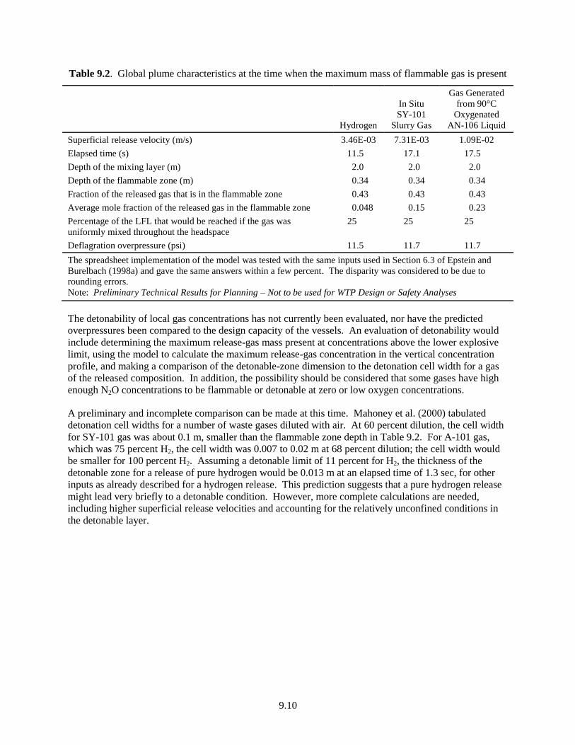
9.10
Table 9.2. Global plume characteristics at the time when the maximum mass of flammable gas is present
Hydrogen
In Situ
SY-101
Slurry Gas
Gas Generated
from 90°C
Oxygenated
AN-106 Liquid
Superficial release velocity (m/s) 3.46E-03 7.31E-03 1.09E-02
Elapsed time (s) 11.5 17.1 17.5
Depth of the mixing layer (m) 2.0 2.0 2.0
Depth of the flammable zone (m) 0.34 0.34 0.34
Fraction of the released gas that is in the flammable zone 0.43 0.43 0.43
Average mole fraction of the released gas in the flammable zone 0.048 0.15 0.23
Percentage of the LFL that would be reached if the gas was
uniformly mixed throughout the headspace
25 25 25
Deflagration overpressure (psi) 11.5 11.7 11.7
The spreadsheet implementation of the model was tested with the same inputs used in Section 6.3 of Epstein and
Burelbach (1998a) and gave the same answers within a few percent. The disparity was considered to be due to
rounding errors.
Note: Preliminary Technical Results for Planning – Not to be used for WTP Design or Safety Analyses
The detonability of local gas concentrations has not currently been evaluated, nor have the predicted
overpressures been compared to the design capacity of the vessels. An evaluation of detonability would
include determining the maximum release-gas mass present at concentrations above the lower explosive
limit, using the model to calculate the maximum release-gas concentration in the vertical concentration
profile, and making a comparison of the detonable-zone dimension to the detonation cell width for a gas
of the released composition. In addition, the possibility should be considered that some gases have high
enough N2O concentrations to be flammable or detonable at zero or low oxygen concentrations.
A preliminary and incomplete comparison can be made at this time. Mahoney et al. (2000) tabulated
detonation cell widths for a number of waste gases diluted with air. At 60 percent dilution, the cell width
for SY-101 gas was about 0.1 m, smaller than the flammable zone depth in Table 9.2. For A-101 gas,
which was 75 percent H2, the cell width was 0.007 to 0.02 m at 68 percent dilution; the cell width would
be smaller for 100 percent H2. Assuming a detonable limit of 11 percent for H2, the thickness of the
detonable zone for a release of pure hydrogen would be 0.013 m at an elapsed time of 1.3 sec, for other
inputs as already described for a hydrogen release. This prediction suggests that a pure hydrogen release
might lead very briefly to a detonable condition. However, more complete calculations are needed,
including higher superficial release velocities and accounting for the relatively unconfined conditions in
the detonable layer.
10.1
10.0 Conclusions
Technical results were documented and progress was made toward developing technical approaches for
addressing each key question given in Section 1.1. Below are conclusions from the preliminary studies.
As noted in Section 2.0 these results are “Preliminary Technical Results for Planning – Not to be used for
WTP Design or Safety Analyses.”
Both the release of buoyant RFID beads and velocity measurements from the UVP-DUO/2 MHz
transducer combination appear promising for being correlated with gas release from sheared
non-Newtonian slurries. Further development is still needed for these approaches to be useful as
mixing metrics for gas release.
Regions of imperfect mixing, or dead zones, can retain and spontaneously release gas. Preliminary
models and an experiment were completed that confirm the expected general behavior. Further
development is needed to provide estimates of allowable dead zone size with reasonable accuracy and
to account for the variation in Hanford waste properties that affect dead zone behavior.
It is unclear if clay simulants used in previous PJM gas release testing at PNNL have reasonably
conservative gas retention and release behavior and further testing and evaluation is needed to defend
the selection of any specific simulant for gas release testing.
BC releases are a significant potential spontaneous release mechanism. Limited test data exist for
materials with rheology in the expected range for WTP non-Newtonian slurries (i.e., Bingham yield
stress between 6 and 30 Pa and consistency between 6 and 30 cP).
Preliminary models and experiments demonstrated significant retention and release events for clay
slurries that were settling concurrently with gas generation with as little as 5 wt% UDS. These
preliminary studies were conducted to demonstrate a technical approach for quantifying the potential
gas retention and release in WTP vessels with relatively low UDS concentration. The approach could
also be used to estimate the maximum amount of solids where there is no possibility for a release to
exceed the LFL in the vessel headspace.
Existing studies on HGR and the physics of gas releases (plumes in the vessel headspace) were
reviewed for determining an approach for evaluating the margin in current estimates of when
sufficient hydrogen gas has been generated to exceed LFL in the vessel headspace. Preliminary
calculations were completed for plume behavior for conditions representative for WTP process
vessels. However, other than this progress on the plume behavior, the approach was not carried
forward to the point of estimating margin in time to LFL in the preliminary studies that were
completed.


11.1
11.0 References
24590-WTP-DB-ENG-01-001, Rev. 2. 2014. Basis of Design. River Protection Project, Waste
Treatment Plant, Richland, Washington.
24590-WTP-ES-ENG-09-001, Rev. 2. 2010. Determination of Mixing Requirements for Pulse-Jet-Mixed
Vessels in the Waste Treatment Plant. River Protection Project, Waste Treatment Plant, Richland,
Washington.
24590-WTP-M4C-V11T-00011. 2010. Revised Calculation of Hydrogen Generation Rates and Times to
Lower Flammability Limit for WTP. River Protection Project, Waste Treatment Plant, Richland,
Washington.
Allen T. 2014. Plan for Resolution of Hydrogen Gas Release from Vessels Technical Issues.
24590-PTF-PL-ENG-14-0012, Rev 1, River Protection Project, Waste Treatment Plant, Richland,
Washington.
Andres UT. 1961. Equilibrium and Motion of Spheres in a Viscoplastic Liquid. Soviet Physics Doklady
(USA), 5, pp 723-726.
Attapatu DD, RP Chhabra, and PHT Uhlherr. 1995. Creeping Sphere Motion in Herschel-Bulkley
Fluids: Flow Field and Drag. Journal of Non-Newtonian Fluid Mechanics, 59, pp 249-265.
Bamberger JA, PA Meyer, JR Bontha, CW Enderlin, DA Wilson, AP Poloski, JA Fort, ST Yokuda,
HD Smith, F Nigl, MA Friedrich, DE Kurath, GL Smith, JM Bates, and MA Gerber. 2005. Technical
Basis for Testing Scaled Pulse Jet Mixing Systems for Non-Newtonian Slurries. PNWD 3551,
WTP-RPT-113 Rev. 0, Battelle-Pacific Northwest Division, Richland, Washington.
Beyler C. 1988. “Chapter 1-17, Flammability Limits of Premixed and Diffusion Flames,” SFPE
Handbook of Fire Protection Engineering, National Fire Protection Association, Inc., Quincy, MA.
Bontha JR, CW Stewart, DE Kurath, PA Meyer, ST Arm, CE Guzman-Leong, MS Fountain, M Friedrich,
SA Hartley, LK Jagoda, CD Johnson, KS Koschik, DL Lessor, F Nigl, RL Russell, GL Smith,
W Yantasee, and ST Yokuda. 2005. Technical Basis for Predicting Mixing and Flammable Gas
Behavior in the Ultrafiltration Feed Process and High-Level Waste Lag Storage Vessels with
Non-Newtonian Slurries. PNWD-3676, WTP-RPT-132, Rev. 0, Battelle-Pacific Northwest Division,
Richland, Washington.
Bredt PR, SM Tingey, and EH Shade. 1995. The Effect of Dilution on the Gas Retention Behavior of
Tank 241-SY-101 Waste. PNL-10781, Pacific Northwest Laboratory, Richland, Washington.
Bredt PR and SM Tingey. 1996. The Effect of Dilution on the Gas Retention Behavior of Tank
241-SY-103 Waste. PNNL-10893, Pacific Northwest National Laboratory, Richland, Washington.
Bryan SA, DM Camaioni, TG Levitskaia, BK McNamara, RL Sell, and LM Stock. 2004. Gas
Generation Testing and Support for the Hanford Waste Treatment and Immobilization Plant.
PNWD-3463, WTP-RPT-115 Rev. 0, Battelle – Pacific Northwest Division, Richland, Washington.
11.2
Burns CA, PA Gauglitz, and RL Russell. 2010. Shear Strength Correlations for Kaolin/Water Slurries:
A Comparison of Recent Measurements with Historical Data. PNNL-19094, Pacific Northwest National
Laboratory, Richland, Washington.
Carothers KG. 1998. Tank 241-C-106 Waste Retrieval Sluicing System Process Control Plan. HNF-SD-
WM-PCP-013, Rev. 0, Fluor Daniel Hanford Inc., Richland, Washington.
Chhabra RP. 1992. Bubbles, Drops, and Particles in Non-Newtonian Fluids. ISBN 0-8493-6718-2.
CRC Press, Inc. Boca Raton, Florida.
CRC. 2011. Handbook of Chemistry and Physics, 92nd Edition, WM Haynes and DR Lide Editors,
CRC Press, Taylor & Francis Group, Boca Raton, Florida.
Daniel RC, JM Billing, CA Burns, RA Peterson, RL Russell, PP Schonewill, and RW Shimskey. 2011.
Filtration Understanding: FY10 Testing Results and Filtration Model Update. PNNL-20299, Pacific
Northwest National Laboratory, Richland, Washington.
Daniel RC, PA Gauglitz, CA Burns, MS Fountain, RW Shimskey, JM Billing, JR Bontha, DE Kurath,
JJ Jenks, PS MacFarlan, and LA Mahoney. 2013. Large-Scale Spray Releases: Additional Aerosol Test
Results. PNNL-22415, WTP-RPT-222 Rev 0, Pacific Northwest National Laboratory, Richland,
Washington.
Daniel RC, CA Burns, AD Crawford, LR Hylden, SA Bryan, PJ MacFarlan, and PA Gauglitz. 2014.
Morphology of Gas Release in Physical Simulants. PNNL-23179, DSGREP-RPT-004 Rev 0, Pacific
Northwest National Laboratory, Richland, Washington.
Eager K, I Tsang, and B Stiver. 2006. Calculation of Hydrogen Generation Rates and Times to Lower
Flammability Limit for WTP. 24590-WTP-M4C-V11T-00004 Rev. C, River Protection Project, Waste
Treatment Plant, Richland, Washington.
Eager K. 2010a. ECCN for Calculation of Hydrogen Generation Rates and Times to Lower
Flammability Limit for WTP. 24590-WTP-M4E-V11T-00009, River Protection Project, Waste Treatment
Plant, Richland, Washington.
Eager K. 2010b. Revised Calculation of Hydrogen Generation Rates and Times to Lower Flammability
Limit for WTP. 24590-WTP-M4C-V11T-00011 Rev. C, River Protection Project, Waste Treatment Plant,
Richland, Washington.
Epstein M, L Swift, and HK Fauske. 1986. “Estimation of Peak Pressure for Sonic-Vented Hydrocarbon
Explosions in Spherical Vessels,” Combustion and Flame 66:1-8.
Epstein M and MG Plys. 1996. "Theoretical Study of Gas Bubble Retention in a Low Yield Stress
Sludge," FAI/96-36, Fauske & Associates, Inc., Burr Ridge, Illinois (May).
Epstein M and JP Burelbach. 1998a. Experimental and Theoretical Turbulent Diffusion Modeling of
Global Light Gas Releases in a Tank Headspace. FAI/98-18 (Feb. 1998), Fauske & Associates, Inc.,
Burr Ridge, Illinois.
Epstein M and JP Burelbach. 1998b. Experimental and Theoretical Turbulent Diffusion Modeling of
Global Light Gas Releases in a Tank Headspace: 2. Local Releases. FAI/98-50 (revised Nov. 1998),
Fauske & Associates, Inc., Burr Ridge, Illinois.
11.3
Gauglitz PA, LA Mahoney, DP Mendoza, and MC Miller. 1994. Mechanisms of Gas Bubble Retention.
PNL-10120, Pacific Northwest Laboratory, Richland, Washington.
Gauglitz PA, SD Rassat, MR Powell, RR Shah, and LA Mahoney. 1995. Gas Bubble Retention and its
Effect on Waste Properties: Retention Mechanisms, Viscosity, and Tensile and Shear Strength.
PNL-10740, Pacific Northwest Laboratory, Richland, Washington.
Gauglitz PA, SD Rassat, PR Bredt, JH Konynenbelt, SM Tingey, and DP Mendoza. 1996. Mechanisms
of Gas Bubble Retention and Release: Results for Hanford Waste Tanks 241-S-102 and 241-SY-103 and
Single-Shell Tank Simulants. PNNL-11298, Pacific Northwest National Laboratory, Richland,
Washington.
Gauglitz PA, G Terrones, SJ Muller, MM Denn, and WR Rossen. 2001. Mechanics of Bubbles in
Sludges and Slurries: Final Report for U.S. Department of Energy. PNNL-13748, Pacific Northwest
National Laboratory, Richland, Washington.
Gauglitz PA, BE Wells, JA Fort, PA Meyer. 2009. An Approach to Understanding Cohesive Slurry
Settling, Mobilization, and Hydrogen Gas Retention in Pulsed Jet Mixed Vessels. PNNL-17707,
WTP-RPT-177 Rev. 0, Pacific Northwest National Laboratory, Richland, Washington.
Gauglitz PA, BE Wells, JA Bamberger, JA Fort, J Chun, and JJ Jenks. 2010a. The Role of Cohesive
Particle Interactions on Solids Uniformity and Mobilization During Jet Mixing: Testing
Recommendations. PNNL-19245, Pacific Northwest National Laboratory, Richland, Washington.
Gauglitz PA, B Buchmiller, JJ Jenks, J Chun, RL Russell, AJ Schmidt, and MM Mastor. 2010b. The
Disruption of Vessel-Spanning Bubbles with Sloped Fins in Flat-Bottom and 2:1 Elliptical-Bottom
Vessels. PNNL-19345, Pacific Northwest National Laboratory, Richland, Washington.
Gauglitz PA, WC Buchmiller, SG Probert, AT Owen, and FJ Brockman. 2012a. Strong-Sludge Gas
Retention and Release Mechanisms in Clay Simulants. PNNL-21167 Rev 0, Pacific Northwest National
Laboratory, Richland, Washington.
Gauglitz PA, DN Tran, and WC Buchmiller. 2012b. Simulant Development for Hanford Double-Shell
Tank Mixing and Waste Feed Delivery Testing. PNNL-21791 Rev 0, Pacific Northwest National
Laboratory, Richland, Washington.
Gimpel R. 2010. Slurry Property Ranges in Non-Newtonian Pretreatment Vessels at WTP.
24590-WTP-RPT-PET-10-014, Rev 2, River Protection Project, Waste Treatment Plant, Richland,
Washington.
Hedengren DC, KM Hodgson, WB Barton, CW Stewart, JM Cuta, and BE Wells. 2000. Data
Observations on Double-Shell Flammable Gas Watch List tank Behavior. RPP-6655, CH2M HILL
Hanford Group, Inc., Richland, Washington.
Hester JR. 2003. Hydrogen Accumulation and Release Behavior of Tank 40H Sludge Slurry.
WSRC-TR-2003-00292 Rev. 0, Westinghouse Savannah River Company, Savannah River Site, Aiken,
South Carolina.
Johnson GD, NW Kirch, RE Bauer, JM Conner, CW Stewart, BE Wells, and JM Grigsby. 2000.
Evaluation of Hanford High-Level Waste Tank 241-SY-101. RPP-6527 Rev. 0, CH2MHILL Hanford
Group, Inc., Richland, Washington.

11.4
Kuhn WL, DR Rector, SD Rassat, CW Enderlin, MJ Minette, JA Bamberger, GB Josephson, BE Wells,
and EJ Berglin. 2013. Scaling Theory for Pulse Jet Mixed Vessels, Sparging, and Cyclic Feed Transport
Systems for Slurries. PNNL-22816, Pacific Northwest National Laboratory, Richland, Washington.
Mahoney LA, ZI Antoniak, JM Bates, and ME Dahl. 1999. Retained Gas Sampling Results for the
Flammable Gas Program. PNNL-13000, Pacific Northwest National Laboratory, Richland, Washington.
Mahoney LA, JL Huckaby, SA Bryan, and GD Johnson. 2000. Overview of the Flammability of Gases
Generated in Hanford Waste Tanks. PNNL-13269, Pacific Northwest National Laboratory, Richland,
Washington.
Mahoney LA and CW Stewart. 2002. Review of the Technical Basis of the Hydrogen Control Limit for
Operations in Hanford Tank Farms. PNNL-13933 Rev. 1, Pacific Northwest National Laboratory,
Richland, Washington.
Mahoney LA, PA Gauglitz, ML Kimura, GN Brown, DE Kurath, J Blanchard, C Song, RC Daniel,
BE Wells, D Tran, WC Buchmiller, CA Burns, and DM Smith. 2013. Small-Scale Spray Releases:
Initial Aerosol Test Results. PNNL-21367, WTP-RPP-216 Rev. 1, Pacific Northwest National
Laboratory, Richland, Washington.
Meacham JE, SJ Harrington, JR Follet, BE Wells, PA Gauglitz, PP Schonewill, MR Powell, and
SD Rassat. 2014. Gas Retention and Release from Hanford Sludge Waste. RPP-RPT-26836 Rev. 1,
Washington River Protection Solutions LLC, Richland Washington.
Meyer PA, LR Pederson, ME Brewster, CW Stewart, SA Bryan, G Terrones, and G Chen. 1997. Gas
Retention and Release Behavior in Hanford Double-Shell Waste Tanks. PNNL-11536 Rev. 1, Pacific
Northwest National Laboratory, Richland, Washington.
Meyer PA and CW Stewart. 2001. Preventing Buoyant Displacement Gas Release Events in Hanford
Double-Shell Waste Tanks. PNNL-13337, Pacific Northwest National Laboratory, Richland,
Washington.
Nasser MS and AE James. 2000. “Settling and sediment bed behavior of kaolinite in aqueous media.”
Sep. Purif. Technol. 51:10-17.
Papp I. 2010. As Received Waste Feed Particle Size and Density. Basis of Design Change Notice.
24590-WTP-BODCN-ENG-10-0003, Waste Treatment Plant, Richland, Washington.
Poloski AP, PA Meyer, LK Jagoda, and PR Hrma. 2004. Non-Newtonian Slurry Simulant Development
and Selection for Pulse Jet Mixer Testing. PNWD-3495, WTP-RPT-111 Rev 0, Battelle--Pacific
Northwest Division, Richland, Washington.
Poloski AP, ST Arm, JA Bamberger, B Barnett, R Brown, BJ Cook, CW Enderlin, MS Fountain,
M Friedrich, BG Fritz, RP Mueller, F Nigl, Y Onishi, LA Schienbein, LA Snow, S Tzemos, M White,
and JA Vucelick. 2005. Technical Basis for Scaling of Air Sparging Systems for Mixing in
Non-Newtonian Slurries. PNWD-3541; WTP-RPT-129, Rev. 0, Battelle–Pacific Northwest Division,
Richland, Washington.
Powell MR, PA Gauglitz, KM Denslow, CM Fischer, DJ Heldebrant, MS Prowant, SA Sande, JM Davis,
and MR Telander. 2014. Evaluation of Gas Retention in Waste Simulants: Intermediate-Scale Column

11.5
and Open-Channel-Depth Tests. PNNL-23136, DSGREP-RPT-003, Pacific Northwest National
Laboratory, Richland, Washington.
Rassat SD, PA Gauglitz, PR Bredt, LA Mahoney, SV Forbes, and SM Tingey. 1997. Mechanisms of Gas
Bubble Retention and Release: Experimental Results for Hanford Waste Tanks 241-AW-101 and
241-AN-103. PNNL-11642, Pacific Northwest National Laboratory, Richland, Washington.
Rassat SD, SM Caley, PR Bredt, PA Gauglitz, DE Rinehart, and SV Forbes. 1998. Mechanisms of Gas
Bubble Retention and Release: Experimental Results for Hanford Single Shell Waste Tanks 241-A-101,
241-S-106, and 241-U-103. PNNL-11981, Pacific Northwest National Laboratory, Richland,
Washington.
Rassat SD, PA Gauglitz, SM Caley, LA Mahoney, and DP Mendoza. 1999. A Discussion of SY-101
Crust Gas Retention and Release Mechanisms. PNNL-12092, Pacific Northwest National Laboratory,
Richland, Washington.
Rassat SD, LM Bagaasen, LA Mahoney, RL Russell, DD Caldwell, and DP Mendoza. 2003. Physical
and Liquid Chemical Simulant Formulations for Transuranic Wastes in Hanford Single-Shell Tanks.
PNNL-14333, Pacific Northwest National Laboratory, Richland, Washington.
Rassat SD, PA Gauglitz, LA Mahoney, RP Pires, DR Rector, JA Fort, GK Boeringa, DN Tran, MR
Elmore, WC Buchmiller, and ML Kimura. 2014. Gas Release Due to Rayleigh-Taylor Instability Within
Sediment Layers in Hanford Double-Shell Tanks: Results of Scaled-Vessel Experiments, Modeling, and
Extrapolation to Full Scale. PNNL-23060 Rev. 1, DSGREP-RPT-002 Rev. 1, Pacific Northwest
National Laboratory, Richland, Washington.
Reynolds DA. 1997. Chemical and Chemically-Related Considerations Associated with Sluicing Tank
C-106 Waste to Tank AY-102. HNF-SD-WM-TI-756, Rev. 2. Lockheed Martin Hanford Corporation,
Richland, Washington.
Russell RL, SD Rassat, ST Arm, MS Fountain, BK Hatchell, CW Stewart, CD Johnson, PA Meyer, and
CE Guzman-Leong. 2005. Final Report: Gas Retention and Release in Hybrid Pulse Jet Mixed Tanks
Containing Non-Newtonian Waste Simulants. PNWD-3552, WTP-RPT-114 Rev. 1, Battelle–Pacific
Northwest Division, Richland, Washington.
Schonewill PP, PA Gauglitz, ML Kimura, GN Brown, LA Mahoney, DN Tran, CA Burns, and
DE Kurath. 2013. Small-Scale Spray Releases: Additional Aerosol Test Results. PNNL-22402,
WTP-RPT-222 Rev. 0, Pacific Northwest National Laboratory, Richland, Washington.
Sherwood DJ and LM Stock. 2004. Modifying the Hu Correlation to Predict Hydrogen Formation in the
Hanford Waste Treatment and Immobilization Plant. 24590-WTP-RPT-RT-04-0002 Rev. 0, River
Protection Project, Waste Treatment Plant, Richland, Washington.
Sherwood DJ. 2008. Evaluation of Potential Gas Release Events in HFP Vessels During Post-Seismic
Period. 24590-HLW-ES-RT-09-001, Rev 2, River Protection Project- Waste Treatment Plant, Richland,
Washington.
Sherwood DJ and AE Sáez. 2014. “The Start of Ebullition in Quiescent, Yield-Stress Fluids.” Nuclear
Engineering and Design 270:101–108.
11.6
Stewart CW, ME Brewster, PA Gauglitz, LA Mahoney, PA Meyer, KP Recknagle, and HC Reed. 1996.
Gas Retention and Release Behavior in Hanford Single-Shell Tanks. PNNL-11391, Pacific Northwest
National Laboratory, Richland, Washington.
Stewart CW, PA Meyer, MS Fountain, CE Guzman-Leong, SA Hartley-McBride, JL Huckaby, and
BE Wells. 2006a. Effect of Anti-Foam Agent on Gas Retention and Release Behavior in Simulated
High-Level Waste. PNWD-3786, WTP-RPT-147, Battelle-Pacific Northwest Division, Richland,
Washington.
Stewart CS, PA Meyer, DE Kurath, and SM Barnes. 2006b. “Scaling Laws for Reduced-Scale Tests of
Pulse Jet Mixing Systems in Non-Newtonian Slurries: Gas Retention and Release Behavior.” In:
Proceedings of Waste Management 2006. February 26–March 2, Tucson, Arizona.
Stewart CW, LA Mahoney, CE Guzman-Leong, JM Alzheimer, ST Arm, JA Bailey, MG Butcher,
SK Cooley, EC Golovich, DE Hurley, LK Jagoda, CD Johnson, WR Park, LD Reid, RW Slaugh,
HD Smith, Y Su, BE Wells, C Wend, and ST Yokuda. 2007. Results from Large-Scale Testing on
Effects of Anti-Foam Agent on Gas Retention and Release. PNNL-17170, WTP-RPT-156 Rev 0, Pacific
Northwest National Laboratory, Richland, Washington.
Van Wylen GJ and RE Sonntag. 1973. Fundamentals of Classical Thermodynamics, 2nd
Ed. John Wiley
and Sons, Inc., New York, NY.
Walker DD, CL Crawford, and NE Bibler. 1994. “Radiolytic Bubble Formation and Level Changes in
Simulated High-Level Waste Salts and Sludges - Application to HLW Storage Tanks.” Proceedings of
Waste Management 1994, Tucson, Arizona, pp. 393-396.
Wells BE, JM Cuta, SA Hartley, LA Mahoney, PA Meyer, and CW Stewart. 2002. Analysis of Induced
Gas Releases During Retrieval of Hanford Double-Shell Tank Waste. PNNL-13782, Pacific Northwest
National Laboratory, Richland, Washington.
Wells BE, MA Knight, EC Buck, RC Daniel, SK Cooley, LA Mahoney, PA Meyer, AP Poloski,
JM Tingey, WS Callaway, GA Cooke, ME Johnson, MG Thien, DJ Washenfelder, JJ Davis, MN Hall,
G Smith, SL Thomson, and Y Onishi. 2007. Estimate of Hanford Waste Insoluble Solid Particle Size
and Density Distribution. WTP-RPT-153, PNWD-3824, Battelle—Pacific Northwest Division, Richland,
Washington.
Wells BE, DE Kurath, LA Mahoney, Y Onishi, JL Huckaby, SK Cooley, CA Burns, EC Buck,
JM Tingey, RC Daniel, and KK Anderson. 2011. Hanford Waste Physical and Rheological Properties:
Data and Gaps. PNNL-20646, Pacific Northwest National Laboratory, Richland, Washington.
Wells BE, SK Cooley, and JE Meacham. 2013. Prediction of Peak Hydrogen Concentrations for Deep
Sludge Retrieval in Tanks AN-101 and AN-106 form Historical Data of Spontaneous Gas Release Events.
PNNL-22866, DSGREP-RPT-001, Pacific Northwest National Laboratory, Richland, Washington.
WRPS. 2009. 2009 Auto-TCR for Tank 241-AY-102. RPP-RPT-42920 Rev. 0. Washington River
Protection Solutions, LLC, Richland, Washington.
Zalosh RG. 1988. “Chapter 2-5, Explosion Protection,” SFPE Handbook of Fire Protection Engineering,
National Fire Protection Association, Inc., Quincy, Massachusetts.
Appendix A –
Specification Sheets for Flow Sensors


A.1
Appendix A
Specification Sheets for Flow Sensors

A.2

A.3
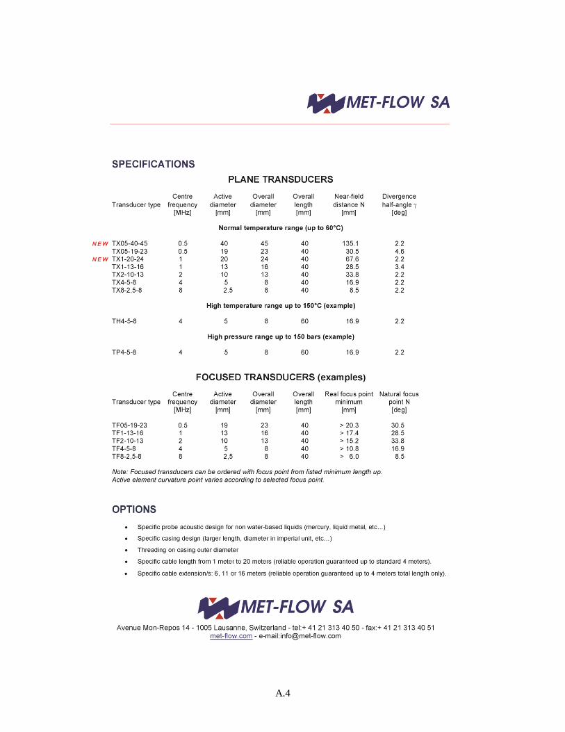
A.4
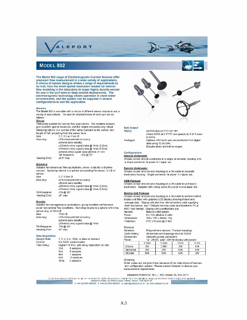
A.5


Appendix B –
Draft Notes for 6/27/14 Meeting

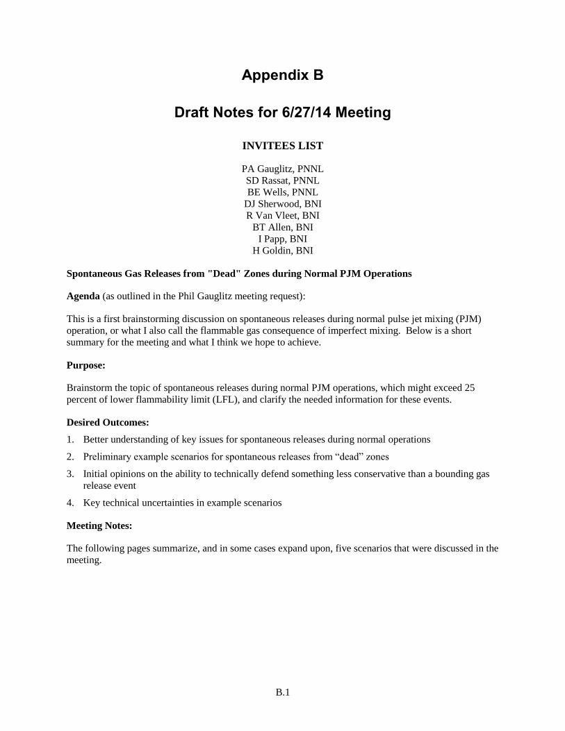
B.1
Appendix B
Draft Notes for 6/27/14 Meeting
INVITEES LIST
PA Gauglitz, PNNL
SD Rassat, PNNL
BE Wells, PNNL
DJ Sherwood, BNI
R Van Vleet, BNI
BT Allen, BNI
I Papp, BNI
H Goldin, BNI
Spontaneous Gas Releases from "Dead" Zones during Normal PJM Operations
Agenda (as outlined in the Phil Gauglitz meeting request):
This is a first brainstorming discussion on spontaneous releases during normal pulse jet mixing (PJM)
operation, or what I also call the flammable gas consequence of imperfect mixing. Below is a short
summary for the meeting and what I think we hope to achieve.
Purpose:
Brainstorm the topic of spontaneous releases during normal PJM operations, which might exceed 25
percent of lower flammability limit (LFL), and clarify the needed information for these events.
Desired Outcomes:
1. Better understanding of key issues for spontaneous releases during normal operations
2. Preliminary example scenarios for spontaneous releases from “dead” zones
3. Initial opinions on the ability to technically defend something less conservative than a bounding gas
release event
4. Key technical uncertainties in example scenarios
Meeting Notes:
The following pages summarize, and in some cases expand upon, five scenarios that were discussed in the
meeting.
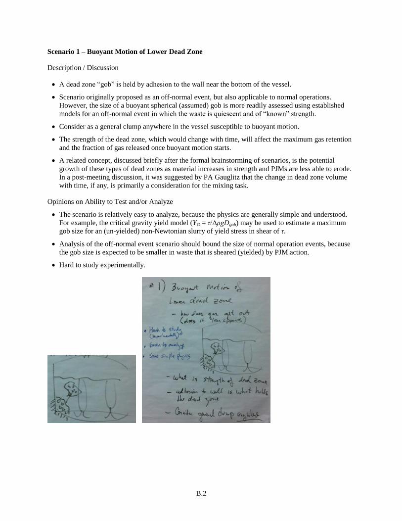
B.2
Scenario 1 – Buoyant Motion of Lower Dead Zone
Description / Discussion
A dead zone “gob” is held by adhesion to the wall near the bottom of the vessel.
Scenario originally proposed as an off-normal event, but also applicable to normal operations.
However, the size of a buoyant spherical (assumed) gob is more readily assessed using established
models for an off-normal event in which the waste is quiescent and of “known” strength.
Consider as a general clump anywhere in the vessel susceptible to buoyant motion.
The strength of the dead zone, which would change with time, will affect the maximum gas retention
and the fraction of gas released once buoyant motion starts.
A related concept, discussed briefly after the formal brainstorming of scenarios, is the potential
growth of these types of dead zones as material increases in strength and PJMs are less able to erode.
In a post-meeting discussion, it was suggested by PA Gauglitz that the change in dead zone volume
with time, if any, is primarily a consideration for the mixing task.
Opinions on Ability to Test and/or Analyze
The scenario is relatively easy to analyze, because the physics are generally simple and understood.
For example, the critical gravity yield model (YG = τ/ΔρgDgob) may be used to estimate a maximum
gob size for an (un-yielded) non-Newtonian slurry of yield stress in shear of τ.
Analysis of the off-normal event scenario should bound the size of normal operation events, because
the gob size is expected to be smaller in waste that is sheared (yielded) by PJM action.
Hard to study experimentally.

B.3
Scenario 2 – Dead Zone Above PJMs
Description / Discussion
Dead zones may accumulate atop PJMs, whether PJMs are located individually or in a central cluster
with a shroud.
Changing waste fill levels, for example during cross-flow ultrafiltration operations in UFP-2, would
lead to air exposure of and stagnation on top of the PJMs (e.g., air spargers in low-flow idle mode).
Gas releases would likely be through a bubble-cascade mechanism.
Opinions on Ability to Test and/or Analyze
It is harder to analyze, because the physics of bubble cascades are not well understood.
There are no simple physical models to bound the analysis.
Post-meeting thought/suggestion – Generalized experiments can be run to develop better fundamental
understanding of spontaneous and mechanically induced bubble-cascade releases as a function of
waste (simulant) physical properties. The effects of additives, such as anti-foaming agents, might
also be investigated.
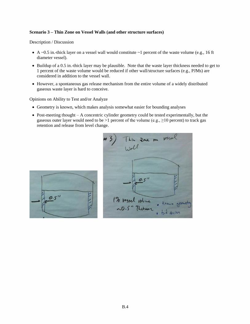
B.4
Scenario 3 – Thin Zone on Vessel Walls (and other structure surfaces)
Description / Discussion
A ~0.5 in.-thick layer on a vessel wall would constitute ~1 percent of the waste volume (e.g., 16 ft
diameter vessel).
Buildup of a 0.5 in.-thick layer may be plausible. Note that the waste layer thickness needed to get to
1 percent of the waste volume would be reduced if other wall/structure surfaces (e.g., PJMs) are
considered in addition to the vessel wall.
However, a spontaneous gas release mechanism from the entire volume of a widely distributed
gaseous waste layer is hard to conceive.
Opinions on Ability to Test and/or Analyze
Geometry is known, which makes analysis somewhat easier for bounding analyses
Post-meeting thought – A concentric cylinder geometry could be tested experimentally, but the
gaseous outer layer would need to be >1 percent of the volume (e.g., ≥10 percent) to track gas
retention and release from level change.

B.5
Scenario 4 – Upper Dead Zone in non-Newtonian Vessel (e.g., more peripheral PJMs)
Description / Discussion
Dead zones in the shadows of peripherally located PJMs and outside the primary PJM mixing zone
Makes less sense if spargers are used, provided that they are placed in, or possibly adjacent to, the
PJM shadows
Opinions on Ability to Test and/or Analyze
Similar to Scenario 2 with a shifted location of the dead zone: with the dead zone near the surface,
bubble cascade and not buoyant motion is the likely release mechanism.
Somewhat easier to analyze, because the size of a dead zone is more readily bounded (e.g., by the
PJM size and location and considering slumping) and because a bubble cascade from an upper dead
zone is less complicated than a bubble cascade from a bottom dead zone.
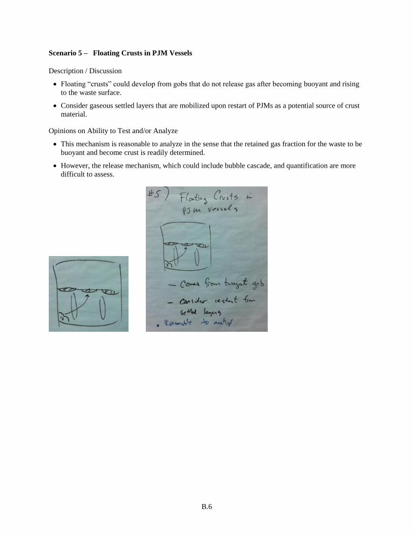
B.6
Scenario 5 – Floating Crusts in PJM Vessels
Description / Discussion
Floating “crusts” could develop from gobs that do not release gas after becoming buoyant and rising
to the waste surface.
Consider gaseous settled layers that are mobilized upon restart of PJMs as a potential source of crust
material.
Opinions on Ability to Test and/or Analyze
This mechanism is reasonable to analyze in the sense that the retained gas fraction for the waste to be
buoyant and become crust is readily determined.
However, the release mechanism, which could include bubble cascade, and quantification are more
difficult to assess.
Appendix C –
Evaluation of Shape Effect for the Buoyant Motion of Dead Zones in Non-Newtonian Yield-Stress Slurries

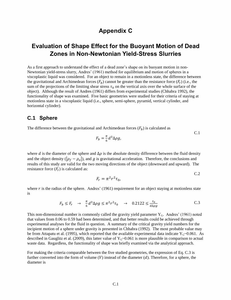
C.1
Appendix C
Evaluation of Shape Effect for the Buoyant Motion of Dead
Zones in Non-Newtonian Yield-Stress Slurries
As a first approach to understand the effect of a dead zone’s shape on its buoyant motion in non-
Newtonian yield-stress slurry, Andres’ (1961) method for equilibrium and motion of spheres in a
viscoplastic liquid was considered. For an object to remain in a motionless state, the difference between
the gravitational and Archimedean forces (𝐹𝑏) cannot be greater than the resistance force (𝐹𝑟) (i.e., the
sum of the projections of the limiting shear stress 𝜏0 on the vertical axis over the whole surface of the
object). Although the result of Andres (1961) differs from experimental studies (Chhabra 1992), the
functionality of shape was examined. Five basic geometries were studied for their criteria of staying at
motionless state in a viscoplastic liquid (i.e., sphere, semi-sphere, pyramid, vertical cylinder, and
horizontal cylinder).
C.1 Sphere
The difference between the gravitational and Archimedean forces (𝐹𝑏) is calculated as
𝐹𝑏 =𝜋
6𝑑3∆𝜌𝑔,
C.1
where 𝑑 is the diameter of the sphere and ∆𝜌 is the absolute density difference between the fluid density
and the object density (|𝜌𝑓 − 𝜌𝑜|), and 𝑔 is gravitational acceleration. Therefore, the conclusions and
results of this study are valid for the two moving directions of the object (downward and upward). The
resistance force (𝐹𝑟) is calculated as:
𝐹𝑟 = 𝜋2𝑟2𝜏0, C.2
where 𝑟 is the radius of the sphere. Andres’ (1961) requirement for an object staying at motionless state
is
𝐹𝑏 ≤ 𝐹𝑟 → 𝜋
6𝑑3∆𝜌𝑔 ≤ 𝜋2𝑟2𝜏0 → 0.2122 ≤
𝜏0
𝑑∆𝜌𝑔 C.3
This non-dimensional number is commonly called the gravity yield parameter YG. Andres’ (1961) noted
that values from 0.06 to 0.59 had been determined, and that better results could be achieved through
experimental analyses for the fluid in question. A summary of the critical gravity yield numbers for the
incipient motion of a sphere under gravity is presented in Chhabra (1992). The most probable value may
be from Attapatu et al. (1995), which reported that the available experimental data indicate YG~0.061. As
described in Gauglitz et al. (2009), this latter value of YG~0.061 is more plausible in comparison to actual
waste data. Regardless, the functionality of shape was briefly examined via the analytical approach.
For making the criteria comparable between the five studied geometries, the expression of Eq. C.3 is
further converted into the form of volume (𝑉) instead of the diameter (𝑑). Therefore, for a sphere, the
diameter is

C.2
𝑑 = (6𝑉
𝜋)
1/3= 1.2407𝑉1/3.
C.4
Substituting Eq. C.4 into Eq. C.3 the criteria becomes
0.2633 ≤𝜏0
𝑉1/3∆𝜌𝑔.
C.5
C.2 Semi-Sphere
Following the same procedure as sphere, the criteria of a semi-sphere (half sphere) staying motionless can
be calculated as
𝐹𝑏 =𝜋
12𝑑3∆𝜌𝑔, 𝐹𝑟 =
1
2𝜋2𝑟2𝜏0,
C.6
𝜋
12𝑑3∆𝜌𝑔 ≤
1
2𝜋2𝑟2𝜏0 → 0.2122 ≤
𝜏0
𝑑∆𝜌𝑔 C.7
It is shown that the form of Eq. C.7 is the same as Eq. C.3, so it may be confusing when comparing the
difficulties of moving a sphere and semi-sphere in viscoplastic liquid. If the Eq. C.7 is converted in to the
form of volume as
𝑑 = (12𝑉
𝜋)
1/3
= 1.5632𝑉1/3 → 0.3317 ≤𝜏0
𝑉1/3∆𝜌𝑔,
C.8
then it is more apparent that a semi-sphere is harder to keep motionless than a sphere if they both have the
same volume. In other words, a semi-sphere is more easily moved by buoyancy force than a sphere in
viscoplastic liquid if they both have volume 𝑉.
C.3 Pyramid
Figure C.1 shows a sketch of the pyramid shape used in this study. Three parameters control the shape
and volume of this category of geometry (i.e., 𝐿, 𝛼, and 𝛽).
Following the same procedure as sphere and semi-sphere, the criteria of a pyramid geometry staying
motionless can be calculated as:
𝐹𝑏 =1
6𝛼𝛽𝐿3∆𝜌𝑔, 𝐹𝑟 = [
𝛽𝐿2
2+ 𝛽𝐿2√𝛼2 +
1
4] 𝜏0,
C.9
1
6𝛼𝛽𝐿3∆𝜌𝑔 ≤ [
𝛽𝐿2
2+ 𝛽𝐿2√𝛼2 +
1
4] 𝜏0 →
1
6
𝛼
1
2+√𝛼2+
1
4
≤𝜏0
𝐿∆𝜌𝑔
C.10
𝐿 = (6𝑉
𝛼𝛽)
1/3
→ 𝛼(
1
𝛼𝛽)
1/3
62/3[0.5+(0.25+𝛼2)1/2]≤
𝜏0
𝑉1/3∆𝜌𝑔,
C.11
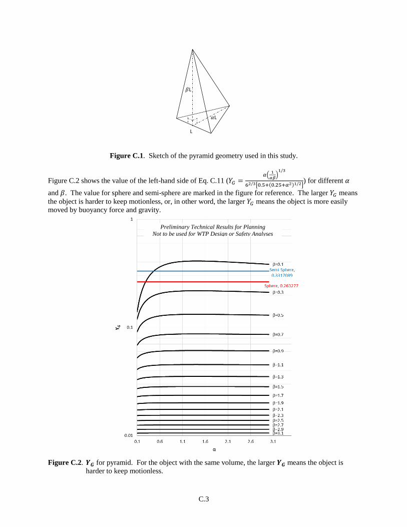
C.3
Figure C.1. Sketch of the pyramid geometry used in this study.
Figure C.2 shows the value of the left-hand side of Eq. C.11 (𝑌𝐺 =𝛼(
1
𝛼𝛽)
1/3
62/3[0.5+(0.25+𝛼2)1/2]) for different 𝛼
and 𝛽. The value for sphere and semi-sphere are marked in the figure for reference. The larger 𝑌𝐺 means
the object is harder to keep motionless, or, in other word, the larger 𝑌𝐺 means the object is more easily
moved by buoyancy force and gravity.
Figure C.2. 𝒀𝑮 for pyramid. For the object with the same volume, the larger 𝒀𝑮 means the object is
harder to keep motionless.
L
L
L
Preliminary Technical Results for Planning
Not to be used for WTP Design or Safety Analyses
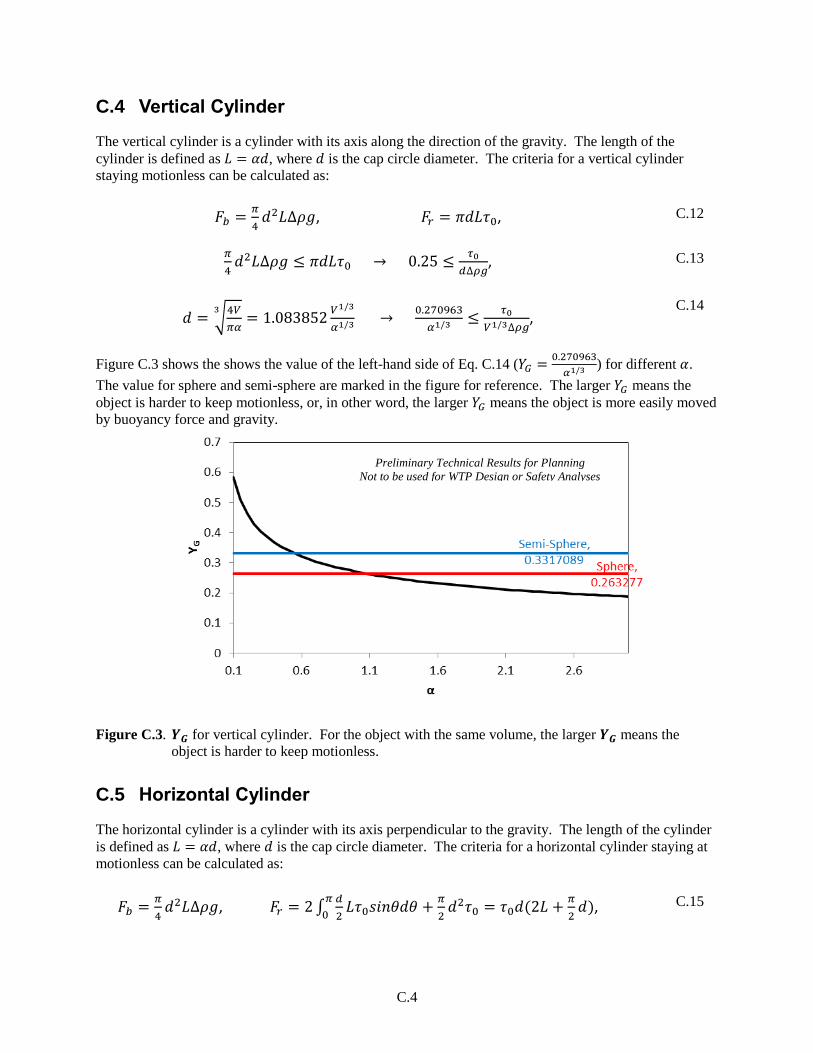
C.4
C.4 Vertical Cylinder
The vertical cylinder is a cylinder with its axis along the direction of the gravity. The length of the
cylinder is defined as 𝐿 = 𝛼𝑑, where 𝑑 is the cap circle diameter. The criteria for a vertical cylinder
staying motionless can be calculated as:
𝐹𝑏 =𝜋
4𝑑2𝐿∆𝜌𝑔, 𝐹𝑟 = 𝜋𝑑𝐿𝜏0,
C.12
𝜋
4𝑑2𝐿∆𝜌𝑔 ≤ 𝜋𝑑𝐿𝜏0 → 0.25 ≤
𝜏0
𝑑∆𝜌𝑔,
C.13
𝑑 = √4𝑉
𝜋𝛼
3= 1.083852
𝑉1/3
𝛼1/3 → 0.270963
𝛼1/3 ≤𝜏0
𝑉1/3∆𝜌𝑔,
C.14
Figure C.3 shows the shows the value of the left-hand side of Eq. C.14 (𝑌𝐺 =0.270963
𝛼1/3 ) for different 𝛼.
The value for sphere and semi-sphere are marked in the figure for reference. The larger 𝑌𝐺 means the
object is harder to keep motionless, or, in other word, the larger 𝑌𝐺 means the object is more easily moved
by buoyancy force and gravity.
Figure C.3. 𝒀𝑮 for vertical cylinder. For the object with the same volume, the larger 𝒀𝑮 means the
object is harder to keep motionless.
C.5 Horizontal Cylinder
The horizontal cylinder is a cylinder with its axis perpendicular to the gravity. The length of the cylinder
is defined as 𝐿 = 𝛼𝑑, where 𝑑 is the cap circle diameter. The criteria for a horizontal cylinder staying at
motionless can be calculated as:
𝐹𝑏 =𝜋
4𝑑2𝐿∆𝜌𝑔, 𝐹𝑟 = 2 ∫
𝑑
2𝐿𝜏0𝑠𝑖𝑛𝜃𝑑𝜃 +
𝜋
2𝑑2𝜏0
𝜋
0= 𝜏0𝑑(2𝐿 +
𝜋
2𝑑),
C.15
Preliminary Technical Results for Planning
Not to be used for WTP Design or Safety Analyses

C.5
𝜋
4𝑑2𝐿∆𝜌𝑔 ≤ 𝜏0𝑑(2𝐿 +
𝜋
2𝑑) → 0.7854 ≤
𝜏0(2𝐿+𝜋
2𝑑)
𝑑𝐿∆𝜌𝑔,
C.16
𝑑 = √4𝑉
𝜋𝛼
3= 1.083852
𝑉1/3
𝛼1/3 → 0.8512575𝛼
(2𝛼+1.5708)𝛼1/3 ≤𝜏0
𝑉1/3∆𝜌𝑔,
C.17
Figure C.4 shows the shows the value of the left-hand side of Eq. C.17 (𝑌𝐺 =0.8512575𝛼
(2𝛼+1.5708)𝛼1/3) for different
𝛼. The value for sphere and semi-sphere are marked in the figure for reference. The larger 𝑌𝐺 means the
object is harder to keep motionless, or, in other word, the larger 𝑌𝐺 means the object is more easily moved
by buoyancy force and gravity.
Figure C.4. 𝒀𝑮 for horizontal cylinder. For the object with the same volume, the larger 𝒀𝑮 means the
object is harder to keep motionless.
For an object with the same volume, the larger 𝑌𝐺 means the object is harder to keep motionless. Based
on this analysis, different dead zone geometries of equal volume may require different gas concentrations
for motion. As noted, the utilized analytical approach differs from experimental results.
C.6 References
Andres UT. 1961. Equilibrium and Motion of Spheres in a Viscoplastic Liquid. Soviet Physics Doklady
(USA), 5, pp 723-726.
Attapatu DD, RP Chhabra, and PHT Uhlherr. 1995. Creeping Sphere Motion in Herschel-Bulkley
Fluids: Flow Field and Drag. Journal of Non-Newtonian Fluid Mechanics, 59, pp 249-265.
Chhabra RP. 1992. Bubbles, Drops, and Particles in Non-Newtonian Fluids, CRC Press, ISBN-13: 978-
0824723293.
Preliminary Technical Results for Planning
Not to be used for WTP Design or Safety Analyses

C.6
Gauglitz PA, BE Wells, JA Fort, PA Meyer. 2009. An Approach to Understanding Cohesive Slurry
Settling, Mobilization, and Hydrogen Gas Retention in Pulsed Jet Mixed Vessels. PNNL-17707, WTP-
RPT-177, Rev. 0. Pacific Northwest National Laboratory, Richland, Washington.

Appendix D –
Non-Newtonian Simulant Properties

D.1
Appendix D
Non-Newtonian Simulant Properties
This appendix provides a summary of the kaolin-bentonite (K:B) slurry simulant properties discussed in
Section 5.5.3. Measured simulant shear strength and rheological properties are compiled in Section D.1
on a batch-by-batch basis. Section D.2 summarizes correlations derived to relate the rheological
properties to the solids content for a number of K:B simulants.
D.1 Measured Shear Strength and Rheological Properties
Measured slurry shear strength and rheological properties for samples taken from batches of K:B simulant
are provided in Table D.1. Entries in Table D.1 are ordered by simulant composition from most to least
kaolin content. Within each simulant type, data are grouped by specific gas release test or test purpose.
Unless otherwise noted, the simulant batches were prepared for the primary purpose of characterization
(see Section 5.5.3) and/or establishing property vs. solids content correlations for use in other testing (see
Section D.2).
See Section 5.5.1 for a summary of the simulant preparation methods. Simulant characterization methods
and instrumentation are described in Section 5.5.2.1, and the Bingham plastic rheology model is
discussed in Section 5.5.2.2.
In many cases, slurry samples were taken from batches at the solids content before addition of hydrogen
peroxide, and, therefore, tabulated data in Table D.1 do not always directly reflect the properties of the
simulant at the final solids concentration used in testing. However, in many cases, small water-dilution
samples at the final solids content were prepared from the stock batch of slurry for characterization.
Table D.1 summarizes the following batch properties: solids mass fraction (xS); measured shear strength
(S) after standing undisturbed (post-mixing) for (typically) 1 hour; and Bingham plastic model yield
stress (0) and consistency (μ∞) obtained from curve fits of rheograms (second down-ramps and up-
ramps). The use of second down-ramp rheogram curve fits is standard; up-ramp data were obtained on a
subset of the samples for comparison, as is discussed in Section 5.5.3.2. Results shown in Table D.1 are
typically for single measurements, but in many cases they are averages of replicate measurements on the
same sample (e.g., shear strength measured in multiple locations) or for multiple portions of the sample
(e.g., to generate unique rheograms). Representative rheograms for several slurries of interest are also
shown in Figure D.1 to Figure D.7. The samples from which the rheograms shown in Figure D.1 to
Figure D.7 were taken are identified in Table D.1.

D
.2
Table D.1. Measured properties for kaolin:bentonite slurry simulant samples (ordered by composition from most to least kaolin content and
grouped by test number or test purpose).
Preliminary Technical Results for Planning – Not to be used for WTP Design or Safety Analyses
Simulant Formulation/
Test Description(a)
Sample(b)
Fraction
Solids, xs
(wt%)
Shear
Strength,(c)
τS (Pa)
Bingham Plastic Model,
Down-Ramp (d)
Bingham Plastic
Model, Up-Ramp (d)
Comments Rheogram
Yield
Stress, τ0
(Pa)
Consistency,
μ∞ (cP)
Yield
Stress,
τ0 (Pa)
Consistency,
μ∞ (cP)
100:0
K:B in
water
Mixing
study
10 min. at Speed 1 081214A 43 18.8 239 82.5 188 126 KitchenAid mixer
with different
speeds and
durations (see
Simulant
Formulation/Test
Description
column)
--
10 min. at Speed 4 081214B 43 29.0 234 76.6 184 119 --
30 min. at Speed 1 081214C 43 30.8 235 74.9 189 121 --
30 min. at Speed 4 081214D 43 49.1 230 75.6 191 112 --
100:0 K:B in water;
Large batches for Tests
FG 23-02 and FG 23-03
23-03-NG-081514 38 12.3 44.4 18.6 37.4 22.7 -- Figure D.1
23-02-GG-072514B-W 39 20.0 n/a n/a n/a n/a --
23-02-GG-072514A-W 43 39.6 n/a n/a n/a n/a --
23-03-Stock-081414 43 26.3 130 48.3 112.1 63.1 --
23-02-GG-072514 48.9 118 632 207 574 287 --
100:0 K:B in water
Settling with gas release
tests
23-05-GG-100914 5.94 n/a n/a
(too low)
1.4 (e)
n/a n/a Measured on pre-
H2O2 samples; the
final solids content
for each was the
closest of 5.0, 10.0,
or 20.0 wt%
--
23-06-GG-101514 11.76 n/a 0.048 (e)
2.2 (e)
n/a n/a --
23-08-GG-110714 11.76 n/a 0.038 2.2 n/a n/a --
092414A 23.6 n/a 0.78 (e)
4.7 (e)
n/a n/a --
092414B 26.4 n/a 1.6 (e)
6.0 (e)
n/a n/a
100:0 K:B in 10-wt% NaCl
Settling with gas release
tests
101314A 6.8 n/a 0.057 (e)
2.6 (e)
n/a n/a --
101314B 13.4 n/a 0.57 (e)
4.2 (e)
n/a n/a --
98:2 K:B in water 102014C 38 6.7 20.0 14.0 16.9 15.5 -- Figure D.6
102014D 44 26.3 96.8 40.9 83.2 50.5 --
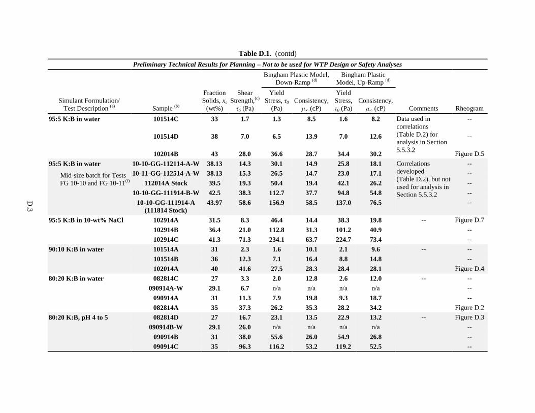
D
.3
Table D.1. (contd)
Preliminary Technical Results for Planning – Not to be used for WTP Design or Safety Analyses
Simulant Formulation/
Test Description (a)
Sample (b)
Fraction
Solids, xs
(wt%)
Shear
Strength,(c)
τS (Pa)
Bingham Plastic Model,
Down-Ramp (d)
Bingham Plastic
Model, Up-Ramp (d)
Comments Rheogram
Yield
Stress, τ0
(Pa)
Consistency,
μ∞ (cP)
Yield
Stress,
τ0 (Pa)
Consistency,
μ∞ (cP)
95:5 K:B in water 101514C 33 1.7 1.3 8.5 1.6 8.2 Data used in
correlations
(Table D.2) for
analysis in Section
5.5.3.2
--
101514D 38 7.0 6.5 13.9 7.0 12.6 --
102014B 43 28.0 36.6 28.7 34.4 30.2 Figure D.5
95:5 K:B in water
Mid-size batch for Tests
FG 10-10 and FG 10-11(f)
10-10-GG-112114-A-W 38.13 14.3 30.1 14.9 25.8 18.1 Correlations
developed
(Table D.2), but not
used for analysis in
Section 5.5.3.2
--
10-11-GG-112514-A-W 38.13 15.3 26.5 14.7 23.0 17.1 --
112014A Stock 39.5 19.3 50.4 19.4 42.1 26.2 --
10-10-GG-111914-B-W 42.5 38.3 112.7 37.7 94.8 54.8 --
10-10-GG-111914-A
(111814 Stock)
43.97 58.6 156.9 58.5 137.0 76.5 --
95:5 K:B in 10-wt% NaCl 102914A 31.5 8.3 46.4 14.4 38.3 19.8 -- Figure D.7
102914B 36.4 21.0 112.8 31.3 101.2 40.9 --
102914C 41.3 71.3 234.1 63.7 224.7 73.4 --
90:10 K:B in water 101514A 31 2.3 1.6 10.1 2.1 9.6 -- --
101514B 36 12.3 7.1 16.4 8.8 14.8 --
102014A 40 41.6 27.5 28.3 28.4 28.1 Figure D.4
80:20 K:B in water
082814C 27 3.3 2.0 12.8 2.6 12.0 -- --
090914A-W 29.1 6.7 n/a n/a n/a n/a --
090914A 31 11.3 7.9 19.8 9.3 18.7 --
082814A 35 37.3 26.2 35.3 28.2 34.2 Figure D.2
80:20 K:B, pH 4 to 5 082814D 27 16.7 23.1 13.5 22.9 13.2 -- Figure D.3
090914B-W 29.1 26.0 n/a n/a n/a n/a --
090914B 31 38.0 55.6 26.0 54.9 26.8 --
090914C 35 96.3 116.2 53.2 119.2 52.5 --
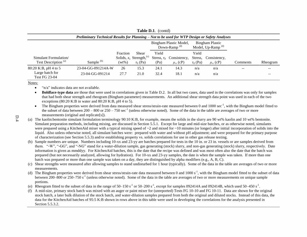
D
.4
Table D.1. (contd)
Preliminary Technical Results for Planning – Not to be used for WTP Design or Safety Analyses
Simulant Formulation/
Test Description (a)
Sample (b)
Fraction
Solids, xs
(wt%)
Shear
Strength,(c)
τS (Pa)
Bingham Plastic Model,
Down-Ramp (d)
Bingham Plastic
Model, Up-Ramp (d)
Comments Rheogram
Yield
Stress, τ0
(Pa)
Consistency,
μ∞ (cP)
Yield
Stress,
τ0 (Pa)
Consistency,
μ∞ (cP)
80:20 K:B, pH 4 to 5
Large batch for
Test FG 23-04
23-04-GG-091214A-W 26 15.3 24.1 14.3 n/a n/a -- --
23-04-GG-091214 27.7 21.0 32.4 18.1 n/a n/a --
Notes:
“n/a” indicates data are not available.
Boldface-type data are those that were used in correlations given in Table D.2. In all but two cases, data used in the correlations was only for samples
that had both shear strength and rheogram (Bingham parameter) measurements. An additional shear strength data point was used in each of the two
exceptions (80:20 K:B in water and 80:20 K:B, pH 4 to 5).
The Bingham properties were derived from data measured shear stress/strain-rate measured between 0 and 1000 sec-1
, with the Bingham model fitted to
the subset of data between 200 – 800 or 250 – 750 sec-1
(unless otherwise noted). Some of the data in the table are averages of two or more
measurements (original and replicate[s]).
(a) The kaolin:bentonite simulant formulation terminology 90:10 K:B, for example, means the solids in the slurry are 90 wt% kaolin and 10 wt% bentonite.
Simulant preparation methods, including mixing, are discussed in Section 5.5.1. Except for large and mid-size batches, or as otherwise noted, simulants
were prepared using a KitchenAid mixer with a typical mixing speed of ~2 and mixed for ~10 minutes (or longer) after initial incorporation of solids into the
liquid. Also unless otherwise noted, all simulant batches were: prepared with water and without pH adjustment; and were prepared for the primary purpose
of characterization (see Section 5.5.3) and/or establishing property vs. solids correlations for use in other gas release testing.
(b) Sample numbers are unique. Numbers including 10-xx and 23-yy are batches prepared for tests in the 10 in. or 23 in. vessels or are samples derived from
them. “-W”, “-GG”, and “-NG” stand for a water-dilution sample, gas generating (stock) slurry, and non-gas generating (stock) slurry, respectively. Date
information is given as mmddyy. For KitchenAid batches, this is the date that the recipe was defined and was most often also the date that the batch was
prepared (but not necessarily analyzed, allowing for hydration). For 10-xx and 23-yy samples, the date is when the sample was taken. If more than one
batch was prepared or more than one sample was taken on a day, they are distinguished by alpha modifiers (e.g., A, B, C).
(c) Shear strengths were measured after allowing samples to stand undisturbed for 1 hour (typically). Some of the data in the table are averages of two or more
measurements.
(d) The Bingham properties were derived from shear stress/strain-rate data measured between 0 and 1000 s-1
, with the Bingham model fitted to the subset of data
between 200–800 or 250–750 s-1
(unless otherwise noted). Some of the data in the table are averages of two or more measurements on unique sample
portions.
(e) Rheogram fitted to the subset of data in the range of 50–150 s-1
or 50–200 s-1
, except for samples 092414A and 092414B, which used 50–450 s-1
.
(f) A mid-size, primary stock batch was mixed with an auger or paint mixer for (unreported) Tests FG 10-10 and FG 10-11. Data are shown for the original
stock batch, a later bulk dilution of the stock batch, and water-dilution samples prepared from both the original and diluted stocks. Instead of this data, the
data for the KitchenAid batches of 95:5 K:B shown in rows above in this table were used in developing the correlations for the analysis presented in
Section 5.5.3.2.
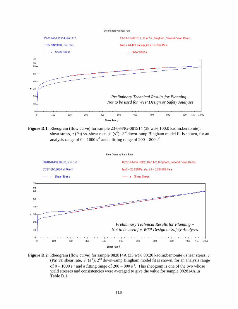
D.5
Figure D.1. Rheogram (flow curve) for sample 23-03-NG-081514 (38 wt% 100:0 kaolin:bentonite);
shear stress, (Pa) vs. shear rate, (s-1
); 2nd
down-ramp Bingham model fit is shown, for an
analysis range of 0 – 1000 s-1
and a fitting range of 200 – 800 s-1
.
Figure D.2. Rheogram (flow curve) for sample 082814A (35 wt% 80:20 kaolin:bentonite); shear stress, (Pa) vs. shear rate, (s
-1); 2
nd down-ramp Bingham model fit is shown, for an analysis range
of 0 – 1000 s-1
and a fitting range of 200 – 800 s-1
. This rheogram is one of the two whose
yield stresses and consistencies were averaged to give the value for sample 082814A in
Table D.1.
0
10
20
30
40
50
60
70
Pa
0 100 200 300 400 500 600 700 800 900 1,0001/s
Shear Rate .
Shear Stress vs Shear Rate
23-03-NG-081514_Run 2-2
CC27-SN13634; d=0 mm
Shear Stress
23-03-NG-081514_Run 2-2_Bingham_Second Down Ramp
tau0 = 44.423 Pa; eta_inf = 0.01859 Pa·s
Shear Stress
0
10
20
30
40
50
60
70
Pa
0 100 200 300 400 500 600 700 800 900 1,0001/s
Shear Rate .
Shear Stress vs Shear Rate
082814A-Pre H2O2_Run 1-2
CC27-SN13634; d=0 mm
Shear Stress
082814A-Pre H2O2_Run 1-2_Bingham_Second Down Ramp
tau0 = 25.829 Pa; eta_inf = 0.034569 Pa·s
Shear Stress
Preliminary Technical Results for Planning –
Not to be used for WTP Design or Safety Analyses
Preliminary Technical Results for Planning –
Not to be used for WTP Design or Safety Analyses
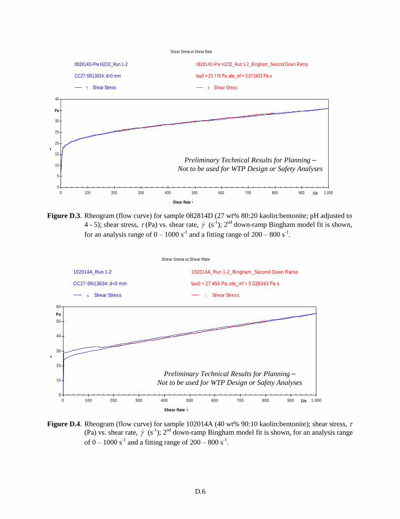
D.6
Figure D.3. Rheogram (flow curve) for sample 082814D (27 wt% 80:20 kaolin:bentonite; pH adjusted to
4 - 5); shear stress, (Pa) vs. shear rate, (s-1
); 2nd
down-ramp Bingham model fit is shown,
for an analysis range of 0 – 1000 s-1
and a fitting range of 200 – 800 s-1
.
Figure D.4. Rheogram (flow curve) for sample 102014A (40 wt% 90:10 kaolin:bentonite); shear stress, (Pa) vs. shear rate, (s
-1); 2
nd down-ramp Bingham model fit is shown, for an analysis range
of 0 – 1000 s-1
and a fitting range of 200 – 800 s-1
.
0
5
10
15
20
25
30
40
Pa
0 100 200 300 400 500 600 700 800 900 1,0001/s
Shear Rate .
Shear Stress vs Shear Rate
082814D-Pre H2O2_Run 1-2
CC27-SN13634; d=0 mm
Shear Stress
082814D-Pre H2O2_Run 1-2_Bingham_Second Down Ramp
tau0 = 23.116 Pa; eta_inf = 0.013452 Pa·s
Shear Stress
0
10
20
30
40
50
60
Pa
0 100 200 300 400 500 600 700 800 900 1,0001/s
Shear Rate .
Shear Stress vs Shear Rate
102014A_Run 1-2
CC27-SN13634; d=0 mm
Shear Stress
102014A_Run 1-2_Bingham_Second Down Ramp
tau0 = 27.454 Pa; eta_inf = 0.028343 Pa·s
Shear Stress
Preliminary Technical Results for Planning –
Not to be used for WTP Design or Safety Analyses
Preliminary Technical Results for Planning –
Not to be used for WTP Design or Safety Analyses

D.7
Figure D.5. Rheogram (flow curve) for sample 102014B (43 wt% 95:5 kaolin:bentonite); shear stress, (Pa) vs. shear rate, (s
-1); 2
nd down-ramp Bingham model fit is shown, for an analysis range
of 0 – 1000 s-1
and a fitting range of 200 – 800 s-1
.
Figure D.6. Rheogram (flow curve) for sample 102014C (38 wt% 98:2 kaolin:bentonite); shear stress, (Pa) vs. shear rate, (s
-1); 2
nd down-ramp Bingham model fit is shown, for an analysis range
of 0 – 1000 s-1
and a fitting range of 200 – 800 s-1
.
0
10
20
30
40
50
60
70
Pa
0 100 200 300 400 500 600 700 800 900 1,0001/s
Shear Rate .
Shear Stress vs Shear Rate
102014B_Run 1-2
CC27-SN13634; d=0 mm
Shear Stress
102014B_Run 1-2_Bingham_Second Down Ramp
tau0 = 36.603 Pa; eta_inf = 0.028736 Pa·s
Shear Stress
0
5
10
15
20
25
30
40
Pa
0 100 200 300 400 500 600 700 800 900 1,0001/s
Shear Rate .
Shear Stress vs Shear Rate
102014C_Run 1-2
CC27-SN13634; d=0 mm
Shear Stress
102014C_Run 1-2_Bingham_Second Down Ramp
tau0 = 20.024 Pa; eta_inf = 0.014002 Pa·s
Shear Stress
Preliminary Technical Results for Planning –
Not to be used for WTP Design or Safety Analyses
Preliminary Technical Results for Planning –
Not to be used for WTP Design or Safety Analyses

D.8
Figure D.7. Rheogram (flow curve) for sample 102914A (31.5 wt% 95:5 kaolin:bentonite in 10 wt%
NaCl); shear stress, (Pa) vs. shear rate, (s-1
); 2nd
down-ramp Bingham model fit is
shown, for an analysis range of 0 – 1000 s-1
and a fitting range of 200 – 800 s-1
.
D.2 Dependence of Rheological Properties on Solids
The slurry rheological property measurements shown in boldface-type in Table D.1 were correlated
versus solids weight fraction for each simulant using an exponential-form curve fit. The resulting
correlations were used, for example, to support calculations of apparent viscosity over a range of shear
rates (Section 5.5.3.2) and determine batch recipes to target simulant physical properties for use in
preliminary gas release tests (e.g., Section 6.3). Table D.2 provides the exponential correlations that were
derived for each simulant for the properties of shear strength, rheogram down-ramp Bingham yield stress,
down-ramp Bingham consistency, up-ramp Bingham yield stress, and down-ramp Bingham consistency.
All correlations shown use solids content, xS, in weight percent (wt%).
0
10
20
30
40
50
60
Pa
0 100 200 300 400 500 600 700 800 900 1,0001/s
Shear Rate .
Shear Stress vs Shear Rate
102914A_Run 1-2
CC27-SN13634; d=0 mm
Shear Stress
102914A_Run 1-2_Bingham_Second Down Ramp
tau0 = 46.416 Pa; eta_inf = 0.014363 Pa·s
Shear Stress
Preliminary Technical Results for Planning –
Not to be used for WTP Design or Safety Analyses

D
.9
Table D.2. Kaolin:bentonite simulant property correlations
Preliminary Technical Results for Planning – Not to be used for WTP Design or Safety Analyses
Simulant
Shear Strength,
S (Pa)
Down-Ramp Bingham Properties Up-Ramp Bingham Properties
Yield Stress, 0
(Pa)
Consistency, μ∞
(cP)
Yield Stress, 0
(Pa)
Consistency, μ∞
(cP)
100:0 K:B 0.00408𝑒0.208𝑥𝑠 0.00404𝑒0.244𝑥𝑠 0.00396𝑒0.221𝑥𝑠 0.00258𝑒0.251𝑥𝑠 0.00310𝑒0.233𝑥𝑠
98:2 K:B 0.00111𝑒0.229𝑥𝑠 0.000930𝑒0.263𝑥𝑠 0.0158𝑒0.179𝑥𝑠 0.000697𝑒0.266𝑥𝑠 0.00863𝑒0.197𝑥𝑠
95:5 K:B 0.000152𝑒0.282𝑥𝑠 0.0000234𝑒0.331𝑥𝑠 0.148𝑒0.122𝑥𝑠 0.0000564𝑒0.310𝑥𝑠 0.102𝑒0.131𝑥𝑠
95:5 K:B, mid-size batch samples(a)
0.00212𝑒0.232𝑥𝑠 0.000385𝑒0.295𝑥𝑠 0.00230𝑒0.230𝑥𝑠 0.000317𝑒0.296𝑥𝑠 0.00117𝑒0.253𝑥𝑠
95:5 K:B in 10 wt% NaCl 0.00797𝑒0.219𝑥𝑠 0.262𝑒0.165𝑥𝑠 0.121𝑒0.152𝑥𝑠 0.134𝑒0.180𝑥𝑠 0.300𝑒0.134𝑥𝑠
90:10 K:B 0.000114𝑒0.321𝑥𝑠 0.0000785𝑒0.318𝑥𝑠 0.291𝑒0.114𝑥𝑠 0.000263𝑒0.290𝑥𝑠 0.241𝑒0.118𝑥𝑠
80:20 K:B 0.00104𝑒0.300𝑥𝑠 0.000369𝑒0.320𝑥𝑠 0.411𝑒0.127𝑥𝑠 0.000799𝑒0.300𝑥𝑠 0.342𝑒0.131𝑥𝑠
80:20 K:B, pH 4 to 5 0.0440𝑒0.219𝑥𝑠 0.102𝑒0.202𝑥𝑠 0.129𝑒0.172𝑥𝑠 0.0897𝑒0.206𝑥𝑠 0.125𝑒0.173𝑥𝑠
Notes:
xs is the solids fraction in weight percent (wt%).
Unless otherwise noted, batches were small enough to prepare using a KitchenAid mixer (Section 5.5.1), and the liquid is water without pH adjustment.
(a) A mid-size, primary stock batch was mixed with an auger or paint mixer for (unreported) Tests FG 10-10 and FG 10-11. The correlation includes data for a
later bulk dilution of the stock batch and water-dilution samples prepared from both the original and diluted stocks. The correlations for KitchenAid batches
shown in the row above were used in the analysis presented in Section 5.5.3.2.


Appendix E –
Proposed 23 in. Diameter Vessel Design


E.1
Appendix E
Proposed 23 in. Diameter Vessel Design
A 23 in. inside diameter (ID) acrylic vessel was designed to help evaluate gas retention and release
behavior of, for example, dead zones of varying shape, size, and location (see Section 6.3). As designed,
the segmented vessel shown in Figure E.1 has interchangeable 2:1 semi-elliptical and flat-bottom heads: a
machined flat plate (e.g., with O-ring grooves) may be inserted above the elliptical bottom when a flat-
bottom configuration is preferred. The design allows the vessel to be filled with simulant to a nominal
2:1 height-to-diameter ratio. In addition, the vessel height was designed considering the clearance of a
floor-stand-mounted overhead mixer when the vessel was placed on a floor scale, for optional mixing
studies. Segmented walls would aid in loading slurries in varying amounts and locations to simulate
theoretical dead zones of concern. For example, a short lower segment could be used to emplace dead
zones near the bottom of the vessel before stacking additional sections and adding the bulk of the
simulant. In addition, cylindrical segments of multiple lengths would help position an unobstructed
viewing area in the region of greatest interest (e.g., to monitor changes in surface level due to gas
retention and release).
One of the challenges in loading test vessels for gas retention and release studies has been layering
supernatant liquid, when used, on top of test slurry. This vessel was designed with an add-on bottom port
(see Figure E.2) to which a bulkhead fitting and a test specific length of tubing could be attached.
Supernatant simulant could be slowly pumped in from the bottom allowing the liquid to spread over the
slurry surface in a less turbulent fashion than some methods of top loading, for example. In addition, the
bottom port was designed to allow the cyclic flow of simulant in and out of the vessel using a reversible
pump system. This could be used to mimic the cyclic level change in the vessel typical of PJM
operations, but without the jet action. Further, a special plug was (conceptually) designed to fit over the
bulkhead fitting and port to create a bottom surface that approximates the contour of the 2:1 elliptical
shape. A “bored through” bulkhead fitting would also be installed in an optional version of the flat-
bottom plate (the other being solid). When used in this configuration, the tube would pass through the
bulkhead fitting in the flat plate and connect with the bulkhead fitting in the elliptical bottom. In both the
elliptical and flat-bottom test arrangements, an elbow would be attached to the lower bulkhead fitting and
connected to a tube running horizontally through a skirt (vessel wall extension) that supports the weight
of the vessel.

E
.2
Figure E.1. Drawings of proposed 23 in. diameter vessel with interchangeable 2:1 semi-elliptical and flat-bottom heads and multiple cylindrical
section lengths.
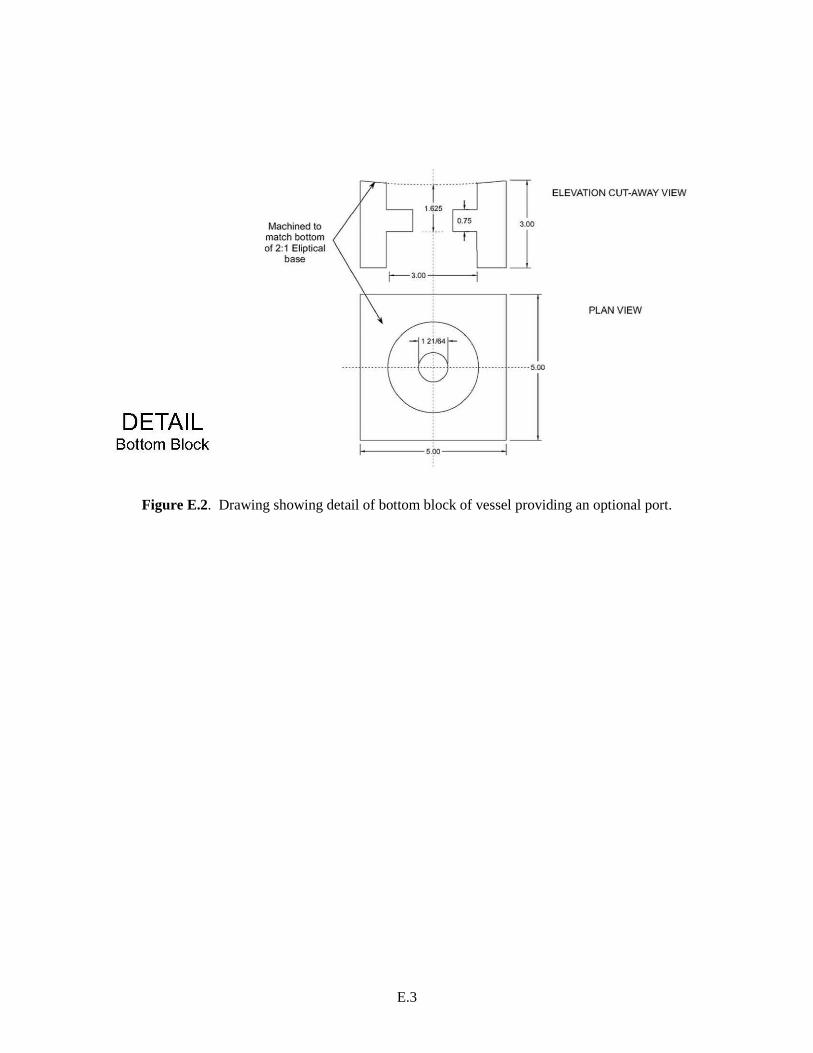
E.3
Figure E.2. Drawing showing detail of bottom block of vessel providing an optional port.


Appendix F –
A Summary of Settling and Rheology Model Work

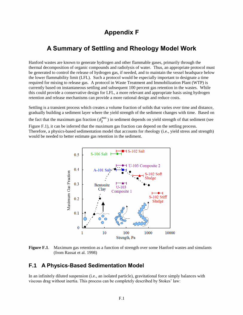
F.1
Appendix F
A Summary of Settling and Rheology Model Work
Hanford wastes are known to generate hydrogen and other flammable gases, primarily through the
thermal decomposition of organic compounds and radiolysis of water. Thus, an appropriate protocol must
be generated to control the release of hydrogen gas, if needed, and to maintain the vessel headspace below
the lower flammability limit (LFL). Such a protocol would be especially important to designate a time
required for mixing to release gas. A protocol in Waste Treatment and Immobilization Plant (WTP) is
currently based on instantaneous settling and subsequent 100 percent gas retention in the wastes. While
this could provide a conservative design for LFL, a more relevant and appropriate basis using hydrogen
retention and release mechanisms can provide a more rational design and reduce costs.
Settling is a transient process which creates a volume fraction of solids that varies over time and distance,
gradually building a sediment layer where the yield strength of the sediment changes with time. Based on
the fact that the maximum gas fraction (maxg ) in sediment depends on yield strength of that sediment (see
Figure F.1), it can be inferred that the maximum gas fraction can depend on the settling process.
Therefore, a physics-based sedimentation model that accounts for rheology (i.e., yield stress and strength)
would be needed to better estimate gas retention in the sediment.
Figure F.1. Maximum gas retention as a function of strength over some Hanford wastes and simulants
(from Rassat et al. 1998)
F.1 A Physics-Based Sedimentation Model
In an infinitely diluted suspension (i.e., an isolated particle), gravitational force simply balances with
viscous drag without inertia. This process can be completely described by Stokes’ law:
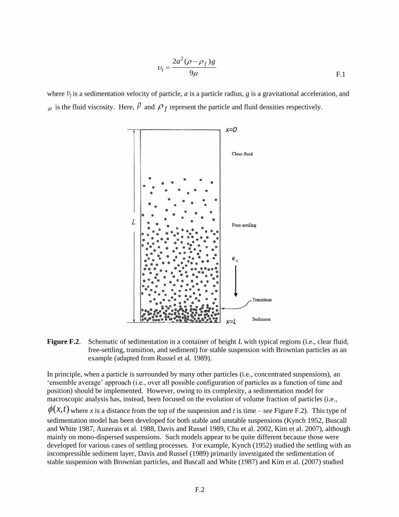
F.2
22 ( )
9
ft
a g
F.1
where t is a sedimentation velocity of particle, a is a particle radius, g is a gravitational acceleration, and
is the fluid viscosity. Here, and f represent the particle and fluid densities respectively.
Figure F.2. Schematic of sedimentation in a container of height L with typical regions (i.e., clear fluid,
free-settling, transition, and sediment) for stable suspension with Brownian particles as an
example (adapted from Russel et al. 1989).
In principle, when a particle is surrounded by many other particles (i.e., concentrated suspensions), an
‘ensemble average’ approach (i.e., over all possible configuration of particles as a function of time and
position) should be implemented. However, owing to its complexity, a sedimentation model for
macroscopic analysis has, instead, been focused on the evolution of volume fraction of particles (i.e.,
( , )x t where x is a distance from the top of the suspension and t is time – see Figure F.2). This type of
sedimentation model has been developed for both stable and unstable suspensions (Kynch 1952, Buscall
and White 1987, Auzerais et al. 1988, Davis and Russel 1989, Chu et al. 2002, Kim et al. 2007), although
mainly on mono-dispersed suspensions. Such models appear to be quite different because those were
developed for various cases of settling processes. For example, Kynch (1952) studied the settling with an
incompressible sediment layer, Davis and Russel (1989) primarily investigated the sedimentation of
stable suspension with Brownian particles, and Buscall and White (1987) and Kim et al. (2007) studied

F.3
the sedimentation of unstable or flocculated suspensions. However, one can understand all sedimentation
models in a unified way, based on mass and momentum conservation equations with all possible stresses
(i.e., gravity, inertia, viscous, and particle stresses). Therefore, this section provides a brief description of
a unified sedimentation model, based on Auzerais et al. (1988), to cover all possible cases.
The behavior of a freely settling suspension is governed by the conservation equation for particles
( ) ( )0
U d U
t x t dx x
,
F.2
where ( )U denotes the sedimentation velocity with x positive measuring downward from an origin at the
top of the liquid (see Figure F.2). To describe a balance between gravity, inertia, viscous, and particle
stresses, a one-dimensional momentum conservation equation, including both fluid and particle phases,
needs to be considered with a relative motion between the liquid and the solid phases
( ) ( )1 1
1 1
ff
C C u uu
t x t x
( )( ) ( )fu gx
F.3
where u and are fluid and particle velocities, respectively. Here ( )C is a virtual mass coefficient as a
function of and is a stress transmitted directly between particles. A drag coefficient, , becomes a
function of in the presence of many neighboring particles, which is defined by
( ) (1 )( )
( )
f g
U
F.4
Note that ( ) 6 a for an isolated particle. Eq. F.3 employs an important physical interpretation: the
first and second terms in left-hand side represent the change of momentum in particles and the action on
the particles of the pressure gradient associated with fluid acceleration. Furthermore, the first, second,
and third terms in right-hand side are the drag force due to relative motion, the difference between gravity
and buoyancy, and the force due to a gradient in , respectively. Therefore, the left-hand side terms
represent a stress associated with inertia and the first, second, and third terms in right-hand side describe
viscous, buoyant, and particle stresses, respectively. Such physical interpretation can be clearer when
scaled equations are used
( )0
U
t x
F.5
and
2( ) ( )
1 11 1
f ft C C u uu
gL t x t x
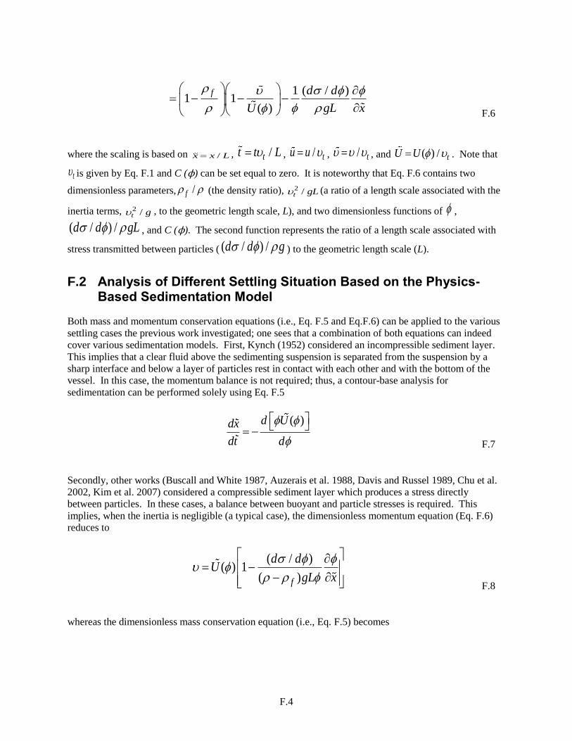
F.4
1 ( / )1 1
( )
f d d
gL xU
F.6
where the scaling is based on /x x L , /tt t L , / tu u , / t , and ( ) / tU U . Note that
t is given by Eq. F.1 and C (ϕ) can be set equal to zero. It is noteworthy that Eq. F.6 contains two
dimensionless parameters, /f (the density ratio), 2 /t gL (a ratio of a length scale associated with the
inertia terms, 2 /t g , to the geometric length scale, L), and two dimensionless functions of ,
( / ) /d d gL , and C (ϕ). The second function represents the ratio of a length scale associated with
stress transmitted between particles ( ( / ) /d d g ) to the geometric length scale (L).
F.2 Analysis of Different Settling Situation Based on the Physics-Based Sedimentation Model
Both mass and momentum conservation equations (i.e., Eq. F.5 and Eq.F.6) can be applied to the various
settling cases the previous work investigated; one sees that a combination of both equations can indeed
cover various sedimentation models. First, Kynch (1952) considered an incompressible sediment layer.
This implies that a clear fluid above the sedimenting suspension is separated from the suspension by a
sharp interface and below a layer of particles rest in contact with each other and with the bottom of the
vessel. In this case, the momentum balance is not required; thus, a contour-base analysis for
sedimentation can be performed solely using Eq. F.5
( )d Udx
dt d
F.7
Secondly, other works (Buscall and White 1987, Auzerais et al. 1988, Davis and Russel 1989, Chu et al.
2002, Kim et al. 2007) considered a compressible sediment layer which produces a stress directly
between particles. In these cases, a balance between buoyant and particle stresses is required. This
implies, when the inertia is negligible (a typical case), the dimensionless momentum equation (Eq. F.6)
reduces to
( / )( ) 1
( )f
d dU
gL x
F.8
whereas the dimensionless mass conservation equation (i.e., Eq. F.5) becomes

F.5
( / )( ) 0
( )f
d dU
t x gL x
F.9
Note that Eqs. F.8 and F.9 with no-flux conditions at the top and bottom of the sedimentation column
constitute a complete description of the settling in this case. Two different types of particle stress are
considered below.
When the suspension is stable and consists of Brownian particles (see Davis and Russel 1989), the
particles would exert an osmotic stress because a Brownian force on the colloidal particles in suspension
is equal to the gradient of osmotic pressure, originated from the inherent non-uniformity of sedimenting
systems. However, solving Eqs. F.8 and F.9 requires constitutive relations for ( )U and ( ) . While
many relations can be suggested, the following relations would be reasonable for suspensions with higher
volume fractions (relevant for typical suspensions) (Auzerais et al. 1988, Davis and Russel 1989)
6.55( ) (1 )U F.10
and
3 3
3 3 1.85( ) ( )
4 4 m
kT kTZ
a a
F.11
where m (=0.64) is the maximum packing density of suspension, ( )Z is known as the compressibility
factor, and kT is the thermal energy.
For unstable (flocculated) suspensions, the physical situation becomes more complicated. At higher
solids concentrations, which are of our major interest, particle interactions can typically produce a
gelation phenomenon where individual flocculants join together into a volume-filling network. As a
result, the particles would exert a compressive yield stress opposing to buoyant stress. Similar to the case
with osmotic stress from particles, the appropriate constitutive relations for ( )U and ( ) are needed.
In this case, the Brinkman permeability, based on the porous medium as a single sphere embedded in an
effective medium, can be used to determine ( )U (Auzerais et al. 1988)
2
2 1/2
(2 3 )( )
3 4 3(8 3 )U
F.12
where the Brinkman permeability (k) is represented by
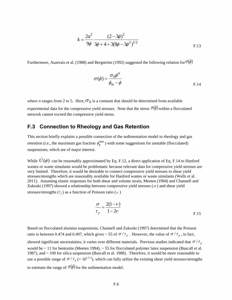
F.6
2 2
2 1/2
2 (2 3 )
9 3 4 3(8 3 )
ak
F.13
Furthermore, Auzerais et al. (1988) and Bergström (1992) suggested the following relation for ( )
0( )n
m
F.14
where n ranges from 2 to 5. Here, 0 is a constant that should be determined from available
experimental data for the compressive yield stresses. Note that the stress ( ) within a flocculated
network cannot exceed the compressive yield stress.
F.3 Connection to Rheology and Gas Retention
This section briefly explains a possible connection of the sedimentation model to rheology and gas
retention (i.e., the maximum gas fraction maxg ) with some suggestions for unstable (flocculated)
suspensions, which are of major interest.
While ( )U can be reasonably approximated by Eq. F.12, a direct application of Eq. F.14 to Hanford
wastes or waste simulants would be problematic because relevant data for compressive yield stresses are
very limited. Therefore, it would be desirable to connect compressive yield stresses to shear yield
stresses/strengths which are reasonably available for Hanford wastes or waste simulants (Wells et al.
2011). Assuming elastic responses for both shear and volume strain, Meeten (1994) and Channell and
Zukoski (1997) showed a relationship between compressive yield stresses ( ) and shear yield
stresses/strengths ( y ) as a function of Poisson ratio ( )
2(1 )
1 2y
F.15
Based on flocculated alumina suspensions, Channell and Zukoski (1997) determined that the Poisson
ratio is between 0.474 and 0.497, which gives ~ 55 of / y . However, the value of / y , in fact,
showed significant uncertainties; it varies over different materials. Previous studies indicated that / y
would be ~ 11 for bentonite (Meeten 1994), ~ 55 for flocculated polymer latex suspension (Buscall et al.
1987), and ~ 100 for silica suspension (Buscall et al. 1988). Therefore, it would be more reasonable to
use a possible range of / y (= 101.5-2
), which can fully utilize the existing shear yield stresses/strengths
to estimate the range of ( ) for the sedimentation model.
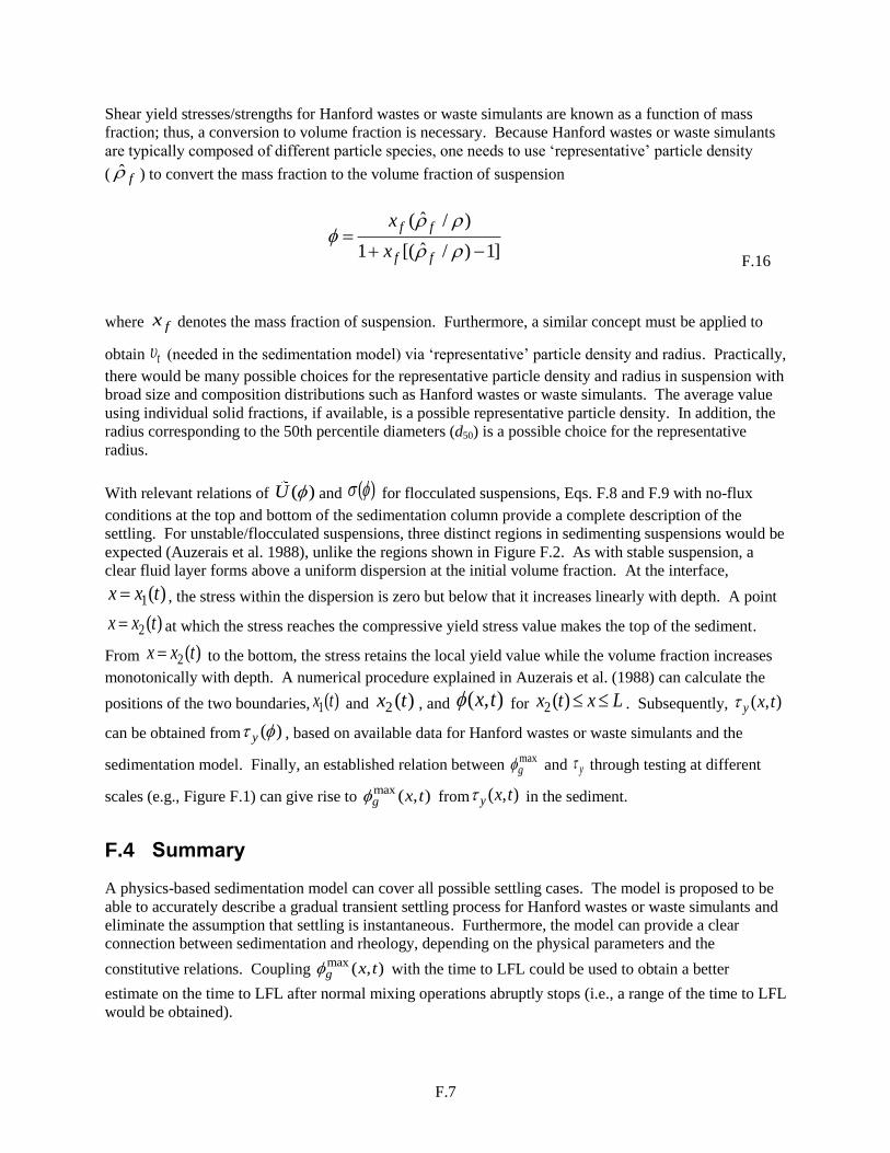
F.7
Shear yield stresses/strengths for Hanford wastes or waste simulants are known as a function of mass
fraction; thus, a conversion to volume fraction is necessary. Because Hanford wastes or waste simulants
are typically composed of different particle species, one needs to use ‘representative’ particle density
( ˆf ) to convert the mass fraction to the volume fraction of suspension
ˆ( / )
ˆ1 [( / ) 1]
f f
f f
x
x
F.16
where fx denotes the mass fraction of suspension. Furthermore, a similar concept must be applied to
obtain t (needed in the sedimentation model) via ‘representative’ particle density and radius. Practically,
there would be many possible choices for the representative particle density and radius in suspension with
broad size and composition distributions such as Hanford wastes or waste simulants. The average value
using individual solid fractions, if available, is a possible representative particle density. In addition, the
radius corresponding to the 50th percentile diameters (d50) is a possible choice for the representative
radius.
With relevant relations of ( )U and ( ) for flocculated suspensions, Eqs. F.8 and F.9 with no-flux
conditions at the top and bottom of the sedimentation column provide a complete description of the
settling. For unstable/flocculated suspensions, three distinct regions in sedimenting suspensions would be
expected (Auzerais et al. 1988), unlike the regions shown in Figure F.2. As with stable suspension, a
clear fluid layer forms above a uniform dispersion at the initial volume fraction. At the interface,
1( )x x t , the stress within the dispersion is zero but below that it increases linearly with depth. A point
2 ( )x x t at which the stress reaches the compressive yield stress value makes the top of the sediment.
From 2 ( )x x t to the bottom, the stress retains the local yield value while the volume fraction increases
monotonically with depth. A numerical procedure explained in Auzerais et al. (1988) can calculate the
positions of the two boundaries, 1( )x t and 2 ( )x t , and ( , )x t for 2( )x t x L . Subsequently, ( , )y x t
can be obtained from ( )y , based on available data for Hanford wastes or waste simulants and the
sedimentation model. Finally, an established relation between maxg and y through testing at different
scales (e.g., Figure F.1) can give rise to max ( , )g x t from ( , )y x t in the sediment.
F.4 Summary
A physics-based sedimentation model can cover all possible settling cases. The model is proposed to be
able to accurately describe a gradual transient settling process for Hanford wastes or waste simulants and
eliminate the assumption that settling is instantaneous. Furthermore, the model can provide a clear
connection between sedimentation and rheology, depending on the physical parameters and the
constitutive relations. Coupling max ( , )g x t with the time to LFL could be used to obtain a better
estimate on the time to LFL after normal mixing operations abruptly stops (i.e., a range of the time to LFL
would be obtained).
F.8
F.5 References
Auzerais FM, R Jackson, WR Russel. 1988. “The Resolution of Shocks and the Effects of Compressible
Sediments in Transient Settling.” J. Fluid Mech. 195: 437-462.
Bergström L. 1992. “Sedimentation of Flocculated Alumina Suspensions: -Ray Measurements and
Comparison with Model Predictions.” J. chem. Soc. Faraday Trans. 88: 3201-3211.
Buscall R and LR White. 1987. “The Consolidation of Concentrated Suspensions.” J. Chem. Faraday
Trans. I 83: 873-891.
Buscall R, IJ McGowan, PDA Mills, RF Stewart, D Sutton, LR White, and GE Yates. 1987. “The
Rheology of Strongly-Flocculated Suspensions.” J. Non-Newtonian Fluid Mech. 24: 183-202.
Buscall R, PDA Mills, JA Goodwin, and DW Lawson. 1988. “Scaling Behaviour of the Rheology of
Aggregate Networks formed from Colloidal Particles.” J. Chem. Soc. Faraday Trans. 84: 4249-4260.
Channell GM and CF Zukoski. 1997. “Shear and Compressive Rheology of Aggregated Alumina
Suspensions.” AIChE J. 43: 1700-1708.
Chu CP, SP Ju, DJ Lee, KK Mohanty. 2002. “Batch Gravitational Sedimentation of Slurries.” J. Colloid
Int. Sci. 245: 178-186.
Davis KE and WR Russel. 1989. “An Asymptotic Description of Transient Settling and Ultrafiltration of
Colloidal Dispersions.” Phys. Fluid A 1: 82-100.
Kim C, Y Liu, A Kühnle, S Hess, S Viereck, T Danner, L Mahadevan, DA Weitz. 2007. “Gravitational
Stability of Suspensions of Attractive Colloidal Particles.” Phys. Rev. Letts. 99: 028303.
Kynch GJ. 1952. “A Theory of Sedimentation.” Trans. Faraday Soc. 48: 166-176.
Meeten GH. 1994. “Shear and Compressive Yield in the Filtration of a Bentonite Suspension.” Coll.
Surf. A 82: 77-83.
Rassat SD, SM Caley, PR Bredt, PA Gauglitz, DE Rinehart, and SV Forbes. 1998. Mechanisms of Gas
Bubble Retention and Release: Experimental Results for Hanford Single Shell Waste Tanks 241-A-101,
241-S-106, and 241-U-103. PNNL-11981, Pacific Northwest National Laboratory, Richland,
Washington.
Russel WB, DA Saville, and WR Schowalter. 1989. Colloidal Dispersions, Cambridge University Press,
New York.
Wells BE, Y Onishi, CA Burns, RC Daniel, DE Kurath, JL Huckaby, EC Buck, KK Anderson, LA
Mahoney, SK Cooley, and JM Tingey. 2011. Hanford Waste Physical and Rheological Properties: Data
and Gaps. PNNL-20646 (EMSP-RPT-006), Pacific Northwest National Laboratory, Richland,
Washington.
PNNL-24255 WTP-RPT-238 Rev. 0
Distribution*
No. of No. of Copies Copies
Dist. 1
ONSITE
2 DOE Office of River Protection
LK Holton H6-60 BM Mauss H6-60
7 Bechtel National Inc.
BT Allen H4-02 HR Hazen H4-02
WF Lenzke III H4-02 SW Schreiber H4-02 DJ Sherwood H4-02
RJ Van Vleet H4-02 WTP PETD Docs H4-02
18 Pacific Northwest National Laboratory
RA Brouns K8-15 JR Bontha K6-28 RC Daniel K6-28
PA Gauglitz (7) K7-15 NK Karri J4-55 LE Mahoney K7-15 LM Peurrung K3-52 SD Rassat K6-28 PP Schonewill K6-28 DN Tran K6-24 BE Wells K7-15
Information Release (pdf) P8-55 Project File K6-28