Hydrodynamical Non-radiative Accretion Flows in

Two-Dimensions

James M. Stone1 James E. Pringle1

1Institute of Astronomy, Cambridge University, Madingley Road, Cambridge CB3 0HA, UK2Department of Astronomy, University of Maryland, College Park, MD 20742 USA

and

Mitchell C. Begelman1,2,3

3JILA, University of Colorado, Boulder, CO 80309-0440 USA4ITP, University of California, Santa Barbara, CA 93106-4030 USA

Received ; accepted

– 2 –

ABSTRACT

Two-dimensional (axially symmetric) numerical hydrodynamical calculationsof accretion flows which cannot cool through emission of radiation are presented.The calculations begin from an equilibrium configuration consisting of a thicktorus with constant specific angular momentum. Accretion is induced by theaddition of a small anomalous azimuthal shear stress which is characterized bya function ν. We study the flows generated as the amplitude and form of ν arevaried. A spherical polar grid which spans more than two orders of magnitudein radius is used to resolve the flow over a wide range of spatial scales. Wefind that convection in the inner regions produces significant outward massmotions that carry away both the energy liberated by, and a large fractionof the mass participating in, the accretion flow. Although the instantaneousstructure of the flow is complex and dominated by convective eddies, long timeaverages of the dynamical variables show remarkable correspondence to certainsteady-state solutions. The two-dimensional structure of the time-averagedflow is marginally stable to the Høiland criterion, indicating that convectionis efficient. Near the equatorial plane, the radial profiles of the time-averagedvariables are power-laws with an index that depends on the radial scaling of theshear stress. A stress in which ν ∝ r1/2 recovers the widely studied self-similarsolution corresponding to an “α-disc”. We find that regardless of the adiabaticindex of the gas, or the form or magnitude of the shear stress, the mass inflowrate is a strongly increasing function of radius, and is everywhere nearly exactlybalanced by mass outflow. The net mass accretion rate through the disc is onlya fraction of the rate at which mass is supplied to the inflow at large radii, andis given by the local, viscous accretion rate associated with the flow propertiesnear the central object.

Subject headings: a

ccretion: accretion discs – black hole physics – hydrodynamics

– 3 –

1. Introduction

There is considerable interest in accretion flows which cannot lose internal energythrough radiative cooling, since they may be relevant to accretion of diffuse plasma ontocompact objects such as black holes and neutron stars. Steady-state solutions for thevertically-averaged radial structure of such flows have been developed within the contextof self-similarity (for example, Ichimaru 1977; Begelman & Meier 1982; Narayan & Yi1994; Abramowicz et al. 1995) assuming angular momentum transport is mediated by ananomalous shear “viscosity”. Solutions in which the mass accretion rate is constant withradius, and in which most of the gravitational binding energy liberated by accretion isstored as thermal energy (often called advection dominated accretion flows, or ADAFs)have been the focus of many recent studies motivated, for example, by the unusually lowhigh-energy luminosity of some accreting black hole candidates (Narayan et al. 1998).

There is, however, a long standing question as to whether vertically-averaged solutionsare indeed a good representation of the true multidimensional flow. For example, it ispossible that the energy liberated by accretion could drive an outflow in the polar regionswhich accompanies accretion at the equator (Narayan & Yi 1994; 1995; Xu & Chen 1997).If the outflow carries a considerable fraction of the mass, energy, and angular momentumavailable in the accretion flow, it will have important consequences for the global nature ofthe solution (for example, the mass inflow rate at the equator can no longer be constant withradius). Recently, steady-state self-similar adiabatic inflow-outflow solutions (or “ADIOS”)have been developed in generality by Blandford & Begelman (1999a; 1999b, hereafter BB).Spectral models of such solutions have been calculated by Quataert & Narayan (1999).Despite the greater generality of the ADIOS models, there remains uncertainty as to howimportant properties of the outflow such as the mass loss rate and terminal velocity aredetermined.

Outflow from a non-radiative accretion flow will only be captured in a multi-dimensionaltreatment of the problem; angle-averaged solutions find only inflow in the inner regions(Ogilvie 1999). In a study of steady flows in thin discs, Urpin (1983; 1984) found thataccretion at the surfaces of the disc could be accompanied by outflow along the equatorial(disc) plane. Gilham (1981) considered two-dimensional self-similar solutions which wereseparable in spherical polar coordinates. His solutions did not contain outflow, but theywere also convectively unstable and therefore could not be steady.

An alternative technique for studying multidimensional non-radiative accretion flowsis to use numerical methods to solve the time-dependent hydrodynamical equationsdirectly. With such methods, a variety of problems related to accretion onto black holeshave been studied. For example, the formation of rotationally supported thick tori frominviscid accretion of gas with various initial angular momentum distributions has beenreported (Hawley, Smarr & Wilson 1984a; 1984b; Hawley 1986; see also Molteni et al.1994; Ryu et al. 1995; Chen et al. 1997). More recently, an accretion flow driven by ananomalous “viscosity” around both non-rotating (Igumenshchev et al. 1996) and rotating(Igumenshchev & Beloborodov 1997) black holes has been simulated, revealing a varietyof interesting features. The dynamic range of spatial scales in these latter simulations istoo small for a direct comparison of the time-averaged state to the steady-state self-similarsolutions discussed above, though more recently these authors have extended theircalculations to include a much larger range in radius (Igumenshchev 1999; Igumenshchev &Abramowicz 1999, hereafter collectively referred to as IA99). These new calculations reveal

– 4 –

that bipolar outflows, strong convection, and quasi-periodic variability can result as thestrength of the viscosity is varied.

Contemporaneous to the latest work of Igumenshchev, we have performed two-dimensional (axisymmetric) hydrodynamic calculations of non-radiative accretion flowswhich span over two orders of magnitude in radius. Our calculations begin with a welldefined initial equilibrium state: a constant angular momentum “thick” torus. Becauseultimately the accretion is driven by an assumed and ad hoc shear stress, we study severaldifferent forms and a wide range of amplitudes for this stress. We find that, for the modelsstudied here, the instantaneous flow is dominated by strong small-scale convection in theinner regions. Some of the time-averaged properties of the flow are remarkably independentof the form of the shear stress, at least for the forms adopted here. In every case we findthat at each radius, the mass flux carried inward by convective eddies is nearly exactlybalanced by outward motions, so that the net mass accretion rate is small compared tothe local mass inflow rate. For some forms of the anomalous stress, the regions of inflowand outflow are distributed equally throughout the disc, while for others the outflow occurspreferentially toward the poles, so that on the largest scales the time-averaged flow forms aglobal circulation pattern of inflow at the equator and slow outflow at the poles. None ofour models show the production of powerful unbound winds. Most importantly, we find thenet mass accretion rate through the disc is determined locally by the properties of the flownear the surface of the inner boundary; it is much smaller than the inflow rate at large radii.

Although our calculations have been pursued independently of the work of IA99, ourformulation of the problem is very similar. In fact we differ only through the use of adifferent numerical method, a different representation of the shear stress (see §2.1), anddifferent initial conditions (see §2.2). It is likely that the only difference of any importanceis the representation of the shear stress. We compare our approach and results in moredetail throughout this paper.

The paper is organized as follows. In §2 we describe our methods. In §3 we presentthe results of our hydrodynamical calculations. In §4 we discuss our results, while in §5 wesummarize and conclude.

2. Method

2.1. The Equations of Motion

To compute the models discussed here, we solve the equations of hydrodynamics

dρ

dt+ ρ∇ · v = 0, (1)

ρdv

dt= −∇P − ρ∇Φ +∇ · T, (2)

ρd(e/ρ)

dt= −P∇ · v + T2/µ, (3)

– 5 –

where ρ is the mass density, P the pressure, v the velocity, e the internal energy density,and T the anomalous stress tensor. The magnitude of the shear stress is determined by thecoefficient µ; we discuss the forms for µ used here below. The d/dt ≡ ∂/∂t + v · ∇ denotesthe Lagrangian time derivative. A strictly Newtonian gravitational potential Φ for a centralpoint mass M is used here. Using a pseudo-Newtonian potential (Paczynski & Wiita 1980)to approximate general relativistic effects in the inner regions is in principle straightforwardbut not of importance to the present investigation. We adopt an adiabatic equation ofstate P = (γ − 1)e, and consider models with both γ = 5/3 and 4/3 (the latter value mayprovide a better, albeit crude, representation of the dynamics of a radiation dominatedfluid). These equations are solved in spherical polar coordinates (r, θ, φ).

The final term on the RHS of equations 2 and 3 represent anomalous shear stress andheating respectively added to drive angular momentum transport and accretion. It mustbe emphasized that the shear stress we wish to approximate is not the result of a truekinematic viscosity. In reality, we expect Maxwell stresses associated with MHD turbulencedriven by the magnetorotational instability (MRI) to provide angular momentum transportin accretion flows (Balbus & Hawley 1998). Modeling such processes from first principlesrequires fully three-dimensional MHD calculations: an important and necessary step forfuture investigations but beyond the scope of this paper. To approximate the effects ofmagnetic stresses, we assume the azimuthal components of the shear tensor T are non-zeroand, in spherical polar coordinates, are given by

Trφ = µr∂

∂r

(vφ

r

), (4)

Tθφ =µ sin θ

r

∂

∂θ

(vφ

sin θ

). (5)

This form is similar to the shear stress in a viscous fluid, in which case µ = νρ is thecoefficient of shear viscosity, and ν the kinematic viscosity coefficient. We emphasize,however, that unlike a viscous fluid, we have assumed the non-azimuthal components ofthe shear stress are zero, because the MRI is driven only by the shear associated withthe orbital dynamics, and therefore we do not expect it to affect poloidal shear to thesame degree. Local three-dimensional MHD simulations of the properties of the MRI inthe non-linear regime confirm that the azimuthal components of the Maxwell stress areindeed more than an order of magnitude larger than the poloidal components (e.g. Hawley,Gammie, & Balbus 1995; 1996; Brandenburg et al. 1995; Stone et al. 1996). IA99 use ashear stress which has a similar form to equations 4 and 5, except they also include thepoloidal stress terms.

Although the local properties of the MRI in the nonlinear regime have been wellstudied, the radial scaling of the Maxwell stresses in a global MHD accretion flow isuncertain. Thus, we adopt several empirical forms for ν to study if and how the flow ischanged. In particular, we consider models with (1) ν ∝ ρ, (2) ν = constant, and (3)ν ∝ r1/2. The first form is adopted primarily as a numerical convenience; it ensures thestresses are confined mostly to the torus where the density is large. In fact, as shown below,it results in a flow with constant density in the equatorial plane, which implies the shearstress per unit volume is nearly constant, i.e. it implies the the solutions for the first andsecond forms of the stress should be similar. The third form for the shear stress correspondsto the expectations of an “α-disc” model. In the last two cases, the stress per volume isindependent of all dynamical variables, thus the flow cannot adjust itself to change T.Thus, we might expect models 2 and 3 to give quite different accretion solutions.

– 6 –

It is important to question whether approximating angular momentum transport inthis manner rather than undertaking the requisite MHD calculations is worthwhile. Because“viscous” non-radiative accretion flows have been so widely discussed in the literature, it isuseful to calculate their time-dependent hydrodynamical evolution over a large spatial scaleboth for comparison to studies of steady-state flows, and to serve as a baseline for futuretime-dependent MHD calculations. Because we find that the time-averaged properties ofthe flow are remarkably independent of the form of the shear stress, it is possible thatsome of the results found here will not be qualitatively different in an MHD calculation,provided the angular momentum transport is dominated by internal Maxwell stress (ratherthan external torques provided by global fields). Clearly MHD calculations are warrantedto investigate these issues.

2.2. Initial Conditions

Our simulations begin with an equilibrium state consisting of a constant angularmomentum torus embedded in a non-rotating, low-density ambient medium in hydrostaticequilibrium. The pressure and density in the torus initially are related through a polytropicequation of state P = Aργ , so that the equilibrium structure of the torus is given by(Papaloizou & Pringle 1984)

P

ρ=

GM

(n + 1)R0

[R0

r− 1

2

(R0

r sin θ

)2

− 1

2d

]. (6)

Here n = (γ−1)−1 is the polytropic index, R0 is the radius of the center (density maximum)of the torus, and d is a distortion parameter which measures the shape of the cross-sectionalarea of the torus. Physical solutions to equation 6 require d > 1, with values near onegiving small, nearly circular cross sections. Without loss of generality, we choose units suchthat G = M = R0 = 1, so that the maximum density is

ρmax =

(1

(n + 1)A

[d− 1

2d

])n

. (7)

For given values of ρmax, d and n, equation 7 determines A. In most cases we adoptρmax = 1, although in some models we specify the mass contained in the torus instead.

The ambient medium in which the torus is embedded has density ρ0 and pressureP0 = ρ0/r. The mass and pressure of the ambient medium should be negligibly small; herewe choose ρ0 = 10−4 so that the ratio of the mass in the ambient medium in r < R0 to thatin the torus Mt is ∼ 4× 10−4. Similarly, the ratio of the maximum pressure in the torus tothe ambient pressure at r = R0 is ∼ 5 × 10−3. In order to guarantee an exact numericalequilibrium initially, we first initialize the density everywhere, and then integrate the radialequation of motion inwards from the outer boundary to compute the pressure using thenumerical difference formula in our hydrodynamics code.

2.3. Numerical Methods

– 7 –

All of the calculations presented here use the ZEUS-2D code described by Stone &Norman (1992). No modifications to the code were required, apart from the addition of theshear stress terms. These terms are updated in an operator split fashion separately from therest of the dynamical equations. For stability, these terms must be integrated using a timestep which satisfies 4t < min(4r, r4 θ)2/ν, where 4r and 4θ are the radial and angulargrid spacing, and the minimum is taken over the entire mesh. Whenever this requirementis smaller than the time step used for the hydrodynamic equations, we sub-cycle: that is weintegrate the viscous terms repeatedly at the smaller timestep until one hydrodynamicaltimestep has elapsed.

Our computational grid extends from an inner boundary at r = RB to 4R0. Inmost simulations, we choose RB = 0.01R0, giving a spatial dynamic range over whichan accretion flow can be established of two orders of magnitude. In some models we setRB = 0.005R0 with the outer boundary at 800RB, so that the grid extends nearly threeorders of magnitude in radius. Such large dynamic ranges are essential for investigatingan accretion flow in the self-similar regime, but are challenging because of the wide rangein dynamical (orbital) timescales. For example, for the standard numerical resolutiongiven below, one orbit of evolution at r = R0 requires 10-15 hours on currently availableworkstations, while calculations at twice the standard resolution take more than 10 timeslonger.

In order to adequately resolve the flow over such a large spatial scale, it is necessary toadopt a non-uniform grid. We choose a logarithmic grid in which (4r)i+1/(4r)i = Nr−1

√10.

This gives a grid in which 4r ∝ r, with Nr grid points per decade in radius. Similarly, inorder to better resolve the flow at the equator, we adopt non-uniform angular zones with(4θ)j/(4θ)j+1 = Nθ−1

√4 for 0 ≤ θ ≤ π/2 (that is the zone spacing is decreasing in this

region), and (4θ)j+1/(4θ)j = Nθ−1√

4 for π/2 ≤ θ ≤ π. This gives a refinement by a factorof four in the angular grid zones between the poles and equator. Equatorial symmetry isnot assumed. Our standard resolution is Nr = 64 and Nθ = 44, giving a grid with a totalsize of 168× 88 zones. We have also computed a high resolution model with Nr = 128 andNθ = 80, giving a grid with a total size of 334× 160 zones.

We adopt outflow boundary conditions (projection of all dynamical variables) atboth the inner and outer radial boundaries. We further set Trφ = 0 at the inner radialboundary. In the angular direction, the boundary conditions are set by symmetry at thepoles (including setting Tθφ = 0).

In some numerical simulations, numerical transport of angular momentum can limitthe accuracy of the results. In fact, the consistent transport algorithms implemented inthe ZEUS-2D code (Stone & Norman 1992) are specifically designed to reduce this effect.As a test, we have evolved a torus with ν = 0 for 2 orbits at r = R0. Apart from a slightsmoothing of the sharp edges of the torus over 2-3 grid zones, we find no evolution. Theangular momentum of the torus is conserved to one part in 106, and the total rotationalkinetic energy to one part in 103.

We have also tested our implementation of the shear stress terms by comparing theevolution of the angle-integrated surface density at early times with the exact analyticsolution for a thin viscous torus (e.g. Figure 1 of Pringle 1981). We find excellentcorrespondence between our numerical and the analytic solution up to a time of roughly 0.8orbits, beyond which effects associated with the multidimensional nature of the flow in oursimulations begin to become important.

– 8 –

3. Results

3.1. A Fiducial Model

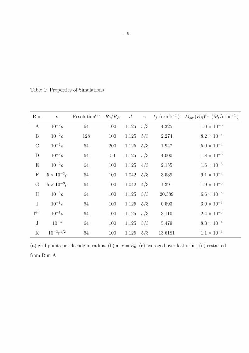
Table 1 summarizes the properties of the simulations discussed here. Columns twothrough six give the coefficient of the shear stress ν, numerical resolution, radial extent ofthe numerical grid expressed as the ratio R0/RB, distortion parameter d of the torus, andadiabatic index γ respectively. The final two columns are the final time tf at which eachsimulation is stopped (all times in this paper are reported in units of the orbital time atr = R0), and the time-averaged mass accretion rate through the inner boundary measurednear the end of the simulation, in units of the initial mass of the torus Mt per orbit.

We find models in which ν ∝ ρ are the quickest to settle into a steady state; we discussthese models in detail to start. Runs A and B are low- and high-resolution simulations of afiducial model with ν = 10−2ρ. Figure 1 plots the time evolution of the density in Run B.In each panel, gray shading is used to denote regions of the torus in which vr > 0. Initially,the evolution is as predicted (Pringle 1981): most of the mass loses angular momentumand falls inward forming a wedge-shaped structure, while a small fraction of the mass gainsangular momentum and moves outward. In fact, as indicated by the shading, the surfacelayers of the inner regions actually move outward – they form a Kelvin-Helmholtz (K-H)roll at the surface of the torus by t = 0.5. By t = 1 material has begun to accrete throughthe inner boundary, while outflow along the surface of the torus has carried the first K-Hroll out to r = 1.75, and a second roll-up is forming at r = 1. Thereafter, the centralwedge-shaped flow thickens considerably, so that by the end of the calculation the densitycontours in the inner regions are nearly radial. The wiggles in the contours in this region arecaused by large amplitude density fluctuations in the flow associated with strong convectivemotions occurring at small radii. This convection drives a low-velocity outflow from theinner regions, in fact, all the material located at angles θ >∼ 45 degrees from the equator isoutflowing. This flow remains bound, however, so that it eventually cascades back onto thesurface of the torus and merges with it in the outer regions. The radial pattern of shadingat t = 2.274 in the inner regions, indicative of alternating columns of material with oppositesign in vr, is another sign of large-scale convective flows.

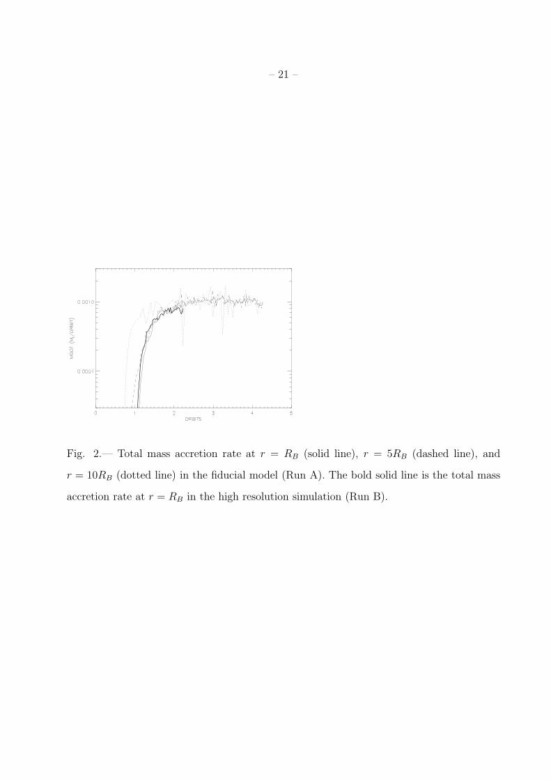
Figure 2 is a plot of the time-history of the angle-integrated mass accretion rate Macc

at r = 0.01 (i.e. the inner boundary), 0.05, and 0.1 in Run A, and at r = 0.01 in Run B,where

Macc(r) = 2πr2∫ π

0ρvr sin θdθ. (8)

Because of the computational expense, Run B has not been evolved beyond 2.274 orbits.Note that the mass accretion rate through the inner boundary converges on the same valueat both resolutions. Moreover, the time-averaged accretion rate is independent of radius atlate times, indicating the flow has reached a steady state over at least one decade in radius.Because the plot shows the integrated accretion rate, it does not reveal the magnitude ofthe inflow near the equator or the outflow near the poles, but only the difference. This netmass accretion rate is very small, it would take Mt/M ≈ 103 orbits to accrete the entiretorus. (Of course some material would never be accreted as required by energy and angularmomentum conservation.)

– 9 –

Table 1: Properties of Simulations

Run ν Resolution(a) R0/RB d γ tf (orbits(b)) Macc(RB)(c) (Mt/orbit(b))

A 10−2ρ 64 100 1.125 5/3 4.325 1.0× 10−3

B 10−2ρ 128 100 1.125 5/3 2.274 8.2× 10−4

C 10−2ρ 64 200 1.125 5/3 1.947 5.0× 10−4

D 10−2ρ 64 50 1.125 5/3 4.000 1.8× 10−3

E 10−2ρ 64 100 1.125 4/3 2.155 1.6× 10−3

F 5× 10−3ρ 64 100 1.042 5/3 3.539 9.1× 10−4

G 5× 10−3ρ 64 100 1.042 4/3 1.391 1.9× 10−3

H 10−3ρ 64 100 1.125 5/3 20.389 6.6× 10−5

I 10−1ρ 64 100 1.125 5/3 0.593 3.0× 10−3

I′(d) 10−1ρ 64 100 1.125 5/3 3.110 2.4× 10−3

J 10−3 64 100 1.125 5/3 5.479 8.3× 10−4

K 10−3r1/2 64 100 1.125 5/3 13.6181 1.1× 10−3

(a) grid points per decade in radius, (b) at r = R0, (c) averaged over last orbit, (d) restarted

from Run A

– 10 –

Fig. 1.— Evolution of the density in a fiducial model (Run B). Time is measured in units

of the orbital time at r = 1. Twenty logarithmic contours are used between the density

maximum (given in each panel) and 10−4. The shaded regions have vr > 0.

– 11 –

To reveal the complex structure of the flow at small radii, in Figure 3 we plot snapshotsof the density, entropy (for a non-radiating fluid) S = ln(P/ργ), and angular momentum

excess compared to Keplerian motion δl = ρ(vφr sin θ −√r sin θ) at t = 1.95 for the centralregion r < 0.1. The complexity of the flow on these scales is evident. Overall, the density isstrongly stratified from the poles to the equator, however on small scales large amplitudefluctuations associated with convection dominate the image. Several regions of dense blobsand filaments (which move inward), and low density bubbles (which move outward) areclearly evident. Note that at some radii, the angular position of the density maximumis displaced far from the equator, an indication of how strongly the convective motionsdominate the flow. The entropy plot shows the generic result for a non-radiative accretionflow that S is maximum along the poles (where the density is a minimum), and smallestalong the equator. However, once again the dominant pattern in the image are the bubblesand filaments associated with convection. Finally, the plot of δl shows that overall, theflow near the poles has an excess of angular momentum compared to Keplerian, while nearthe equator large amplitude fluctuations of both excess and deficit are present. A plot ofthe instantaneous radial velocity on these scales is complex, revealing that both inflow andoutflow occurs at some place along most radial slices. However, there is an overall patternto the flow: inflow dominates near the equator and outflow near the poles. Comparison ofthe three images demonstrates that, as one would expect, regions of highest density (whichare observed to move inward) have low S and a deficit of angular momentum, while bubblesof low density (which are observed to move outwards) have high S and an excess of angularmomentum. A detailed comparison of the properties of convection in a rapidly rotatingflow such as being studied here with the known properties of stellar convection (e.g. Mestel1999) would be fruitful, but will not be discussed further here.

In order to investigate the time-averaged properties of the flow, in Figure 4 we plotcontours of a number of time-averaged quantities, including the specific angular momentumL = vφr sin θ, and the Bernoulli function B ≡ v2/2 + γP/(γ − 1)ρ − r−1. The latter isshaded in regions where B < 0. These averages are constructed from 139 equally spaceddata files between orbits 2.0 and 2.278. The time-averaged variables form remarkablysimple patterns compared to the instantaneous snapshots (c.f. Fig. 3). In each case thecontours form smooth curved surfaces which are symmetric with respect to the equator.The ordering of the variables according to the shape of their contours (from concave toconvex with respect to an outward radial norm) is ρ, P , r, Ω, R L, B, and S, where r andR are spherical and cylindrical radial coordinates respectively. Contours of the last threevariables are in fact virtually parallel, except for contours of B < 0. (Note in the regionshown the contours of ρ are nearly radial, however since they must close at large r weconsider this as an extreme limit of concavity.) This ordering is precisely that expected forstability against the Høiland criterion (Begelman & Meier 1982; BB), thus we conclude themean state is marginally stable. The convective motions are therefore so efficient as to drivethe mean flow to marginal stability (since the instantaneous structure is clearly unstable).We note the shading of B indicates that in a time-average sense, B < 0 for material nearthe equator (where there is inflow), while B > 0 nearer the poles (where there is outflow).The instantaneous structure of B may contain large bubbles of positive value embedded innegative values near the midplane.

Figure 5 plots the radial structure of the time-averaged flow near the equatorial planein Run B, averaged from θ = 84 to 96 degrees. The time-averaging used to construct theplot is identical to that used in Fig. 4. It is clear that each variable in the plot can bedescribed by a radial power law, with ρ ∝ r0, P ∝ r−1, vφ ∝ r−1/2, and vr ∝ r−1. Note the

– 12 –

rotational velocity never falls below 0.9 times the Keplerian value, except directly next tothe inner boundary. The power-law index of P is somewhat uncertain: P ∝ r−1 is reallyonly a good fit for r < 0.1. If we adopt the ansatz that the Bernoulli function is zero atall radii near the equatorial plane (justified by the results shown in Fig. 4), and that thekinetic energy is dominated by the rotational velocity (which is nearly Keplerian), onewould predict

γP/ρ =1

3r(9)

for γ = 5/3. In fact, equation 9 provides an approximate fit to the radial profile of thetime-averaged C2

s ≡ γP/ρ.

The result that vr ∝ r−1 indicates the solution is not strictly self-similar. Since at r = 1the ratio vr/vφ ∼ 10−2.5, the solution implies (if continued inward) that vr ∼ vφ at r ∼ 10−5.We expect at this point the flow will change qualitatively. The particular scaling of theradial velocity with radius in this flow undoubtedly is related to the form of the shear stressused in this model, ν ∝ ρ ∝ r0. We note that since (from Fig. 5) the ratio C2

s /Ω ≈ 0.3r1/2,it is not possible to characterize the shear stress by a constant αeff = νΩ/C2

s . Instead,αeff ≈ 10−2r−1/2.

Figure 6 plots the radial structure of the time-averaged and angle-integrated massinflow and outflow rates (Min and Mout respectively), defined as

Min(r) = 2πr2∫ π

0ρ min(vr, 0) sin θdθ (10)

Mout(r) = 2πr2∫ π

0ρ max(vr, 0) sin θdθ (11)

as well as the net mass accretion rate Macc defined in equation 8. Clearly Macc = Mout +Min.To construct the plot, we time average the integral (rather than integrating the time-averages) using the same data as in Fig. 4. It is evident that both Min and Mout increase

roughly in proportion to r. However, the difference between the two (Macc) is constantwith radius and is roughly equal to the local mass accretion rate expected for a thin,viscous disc calculated using the properties of the flow near the inner boundary, that isMacc ≈ πν(RB)Σ(RB). Using the known form of the stress ν = 10−2ρ, and the result fromour simulations (see Figs. 5 and 7) that ρ ≈ 0.2 sin θ to compute Σ(RB) gives a viscousmass accretion rate which is within a factor of two of the measured Macc.

Figure 7 plots the angular structure of the time-averaged flow at radial positionsof r = 0.02, 0.05, 0.1, and 0.2, again using the same time-averaging as in Fig. 4. Theangular structure of both the density and pressure shows smooth variation from the polesto equator, with the amplitude of ρ virtually identical at each radius and the amplitude ofP dropping as r−1. The radial velocity is negative over most θ at r = 2RB. At larger rthere are still large variations in vr, despite the large amount of data used to construct thetime-average. The average vr is slightly negative within about 30 degrees of the equator,and strongly positive within 50 degrees of the poles. The rotational velocity vφ is nearlyconstant with θ at every radial position, so that L varies as sin θ. From the plots it isdifficult to distinguish a surface that might be used to define the accretion disc as opposedto the polar outflow. Crudely, a surface might be defined near θ = 45 degrees where the

– 13 –

time-averaged radial velocity changes sign. Alternatively, the surface of B = 0 in the fifthpanel of Fig. 4 might be considered to define a disc.

A plot of the time-averaged angular velocity reveals vθ is negative (positive) within 50degrees of θ = 0 (θ = π), and nearly zero elsewhere. The angular and radial pattern of vr

and vθ indicate that for Run B, there is a weak global circulation pattern consisting of slowradial infall near the equator, and faster polar outflow above θ ≈ 45 degrees. The averagevelocity of the circulation is much smaller than the instantaneous fluctuations, especiallynear the equator.

The increase of Min and Mout with radius indicates most of the mass which flows inwardnear the equatorial plane eventually flows outward towards the poles. Fundamentally, thisresult seems to be a consequence of strong convection in the inner regions which, whencombined with diffusion on the smallest scales, serves to mix the specific entropy of thefluid. Thus, outflowing material has only a slightly larger specific entropy than the rest ofthe material, so that it is very inefficient at carrying away energy liberated by the infallinggas (BB). The result is that a large amount of outflowing mass is required to remove theenergy liberated by the small accretion rate.

To confirm that our solution is independent of the location of the inner boundary,we have calculated the evolution of two additional models, one with RB = 0.005 (RunC), and the other with RB = 0.02 (Run D), but otherwise identical to Run A. The final,

time-averaged Macc through the inner boundary measured from these runs is listed inTable 1. The results are consistent with Macc ∝ r. Since for the particular accretion flowestablished in our simulations the viscous accretion rate is proportional to r, this resultagain indicates that the net mass accretion rate is determined locally at the surface of thecentral object. The details of the flow in Runs C and D are similar to Run A, we find thesame radial and angular structure of the time-averaged flow as is shown in Figs. 4-7. Inparticular, the outflowing material is still bound, and has the same total energy as in RunA, and therefore stagnates at roughly the same radial position as the flow shown in the lastpanel of Fig. 1. Making the inner boundary smaller does not lead to the production of amore energetic outflow. Of course, varying the location of the inner boundary is equivalentto moving the initial location of the torus either closer to or farther from the central pointmass. Since most of the gravitational energy is liberated near the central object, we shouldnot expect substantial changes in the flow if the torus starts at 200RB as opposed to 100RB,as is indeed observed.

We have studied the direction of the time-averaged advective flux of mass, energy,and angular momentum, and the flux of L transported by shear stresses in Run B. Wefind the first three are nearly identical, thus in Figure 8 we show a vector plot of onlyM = 2πr2ρvr sin θ for the same 139 data files as used to construct Figs. 4-7. To furtherreduce the noise in the data, we have averaged together the fluxes on either side of theequator. Even so, the direction of the inflow does not form smooth streamlines. Overall,there is a quasi-radial inflow within θ ∼ 45 degrees, and a more nearly radial outflow abovethat (although, consistent with the profile of the time-averaged angular velocities mentionedabove, the mass flux vectors are more polar than equatorial). Note from Fig. 8 that onecould also use the change in sign of the radial component of the average mass flux vectorsto crudely define a surface to the disc at θ ∼ 45 degrees. Although not plotted, the viscousflux of angular momentum is radial within the inflowing regions, and away from the polesin the outflow.

– 14 –

The accretion flow which emerges from these calculations must be driven by angularmomentum transport associated with the anomalous shear stress. This is clearlydemonstrated by setting the shear stress to zero once the mass accretion rate has reached asteady-state. When Run A is continued for another orbit with ν = 0, the mass accretionrate drops by an order of magnitude within 0.1 orbits, the convective motions die away,and the torus settles into a new two-dimensional hydrostatic equilibrium with a nearlyKeplerian rotation profile near the equator.

It can also be demonstrated that the thermal heating due to the anomalous shearstress plays a fundamental role in producing convection and mass outflow. If we repeatthe fiducial model with the heating term (last term in equation 3) removed, we find ahigh-velocity, ordered infall is produced with no small-scale convective motions.

We have studied the effect of varying the adiabatic index γ on the properties of theflow. Run E listed in Table 1 has γ = 4/3, but otherwise is identical to the fiducial modelRun A (a different value of A must be chosen in order to keep Mt fixed – this increases themaximum initial density in the torus). We find that apart from being slightly more compactin the equatorial plane (the opening angle of the accretion being closer to 30 degrees)the detailed properties of the solution (for instance the radial scaling of time-averagedvariables) do not change significantly compared to Run A. The rotational velocity is stillvery nearly Keplerian, and ρ ∝ r0 and vr ∝ r−1. Most significantly, we still find Min ∝ rin this simulation. The mass accretion rate through the inner boundary listed in Table 1 isincreased in Run E compared to A; it is a small fraction of Min(R0) and is consistent withthe local, viscous accretion rate at the inner boundary.

Finally, to study the effect of the shape of the initial torus, we have computed twomodels with d = 1.042, one with γ = 5/3 (Run F) and one with γ = 4/3 (Run G). Onceagain, Mt is kept fixed between these models by choosing an appropriate value for A. Thesmaller value of d used in these models gives the torus in the initial state a cross-sectionaldiameter about one half the value in Run A. We find no qualitative change in the solutioncompared to Run A. In particular, the outflow is driven to the same radial position (butno farther), indicating that the initial thermal energy is not important in the outflow. Inboth cases, the flow is dominated by convection in the inner regions, with time-averagedradial profiles for each variable that obey the same radial scalings as found for Run A. Theγ = 5/3 (Run F) model has a steady-state mass accretion rate identical to Run A, while inthe γ = 4/3 (Run G) model the accretion rate is increased by the same amount as Run E.

3.2. Effect of varying the amplitude of the Shear Stress

We have calculated the evolution of two models in which ν = 10−3ρ and ν = 10−1ρ (i.e.,the shear stress is either ten times smaller or larger than in the fiducial model respectively).These models are labeled as Runs H and I in Table 1. Each model is computed at thestandard resolution of 64 grid points per decade in radius. Together with Run A, they forma set of models which span two orders of magnitude in amplitude of the anomalous shearstress.

At low values of the shear stress (Run H), the evolution to a steady accretion flowproceeds much more slowly than in the fiducial model, as one would expect. Thus, it takes

– 15 –

roughly 20 orbits of the torus for Macc to converge to a steady value. This value (finalcolumn in Table 1) is roughly fifteen times smaller than Run A, although for a viscous discone expects the mass accretion rate to be directly proportional to ν. The discrepancy canbe attributed to the fact that the density at the equator is about 2/3 the value in Run A.The two-dimensional structure of the time-averaged flow in Run H is very similar to thatshown in Figure 4 for Run A. The radial scaling of all variables near the equator also followthe results of Run A closely, i.e. ρ ∝ r0, P ∝ r−1, vφ ∝ r−1/2, and vr ∝ r−1. The ratioof vr/vφ ∼ 10−3 at R0, slightly smaller than Run A. Once again, the inner regions of theflow are dominated by convective motions which drive a significant outward mass flux thatcarries away most of the energy liberated by accretion. The mass inflow rate once againscales as Min ∝ r.

At high values of the shear stress (Run I), the evolution of the torus becomes verydynamic. In fact, the initial infall of material from the torus becomes nearly supersonic,reaching the rotation axis after only 0.15 orbits. This rapid infall creates a high pressureas material reflects off the rotation axis, resulting in the ejection of some matter along thepoles. Convective motions begin within r < 0.1 after 0.2 orbits, at which point the flowattempts to settle into the same equatorial-inflow polar-outflow solution observed in RunA. However, the mass accretion rate is marked by large amplitude fluctuations throughoutthe evolution of Run I, leading to a time-averaged value only 3 times larger than Run A.The time-averaged radial scaling of all variables shows the same dependences on r for allvariables as observed in Run A for r > 0.1, however for r < 0.1 some variables diverge fromsimple power-law behavior. For example, both the rotational and radial velocity becomesflat for r < 0.04. At the inner edge, the ratio of vr/vφ ≈ 0.5, and vφ/Cs ≈ 0.5 (note forRun A this latter ratio ∼ 1.2). These ratios indicate the flow has deviated from strictlyKeplerian rotation, and that radial pressure gradients are playing an important role inthe radial structure of the flow. Despite the fact that the flow at such large values of theshear stress (the “effective-α” of Run I at the inner boundary is αeff = νΩ/C2

s ≈ 0.1) isqualitatively different in the inner regions compared to the fiducial model, we still observevery low mass accretion rates through the inner boundary compared to the mass inflow rateat large radii Min(R0).

Because the violent initial collapse of the torus may be interfering with theestablishment of a steady accretion flow, we have also calculated a model which begins fromthe final state of Run A, but with a shear stress which is slowly increased until ν = 10−1ρ.That is, starting from time 4.325 in Run A, the model is evolved for roughly one orbit withν = 2×10−2ρ, one orbit with ν = 5×10−2ρ, and finally one orbit with ν = 10−1ρ. The finaltime-averaged mass accretion rate in the model (Run I′) given in Table 1 is only a factorof 2.4 larger than the initial accretion rate measured in Run A. In fact, almost no changein the accretion rate is observed after the final increase in ν, indicating that the massaccretion rate is limited at large values of the stress. The radial profiles of each variablein Run I′ follow power laws over a wider range in radii, with vr and vφ becoming flat onlyover r < 0.02. The ratio of vr/vφ ≈ 0.3 at the inner edge, while vφ/Cs ≈ 0.7. The flow inRun I′ is again marked by large amplitude fluctuations in the mass accretion rate. Thus,we conclude that at high values of the shear stress, the flow deviates from a rotationallysupported disc due to radial pressure support. However, we emphasize that strong massoutflow and convection are still important.

Finally, we note that IA99 have also studied the effect of varying the amplitude ofthe shear stress on non-radiative accretion flows. At low values of ν, they find strong,

– 16 –

small-scale convective eddies dominate the flow, in accordance with the results presentedhere. At large ν (much larger than the largest value we have studied here), they find theflow becomes more laminar, and produces a bipolar outflow structure. Qualitatively, ourresults are in agreement, although there is an indication of stronger convection in oursolutions at large ν. It is possible that the poloidal shear stress used by IA99 may partiallysuppress convection in this case.

3.3. Effect of Varying the Form of the Shear Stress

The last two models listed in Table 1 have been computed with entirely different formsfor the anomalous shear stress than Runs A through I discussed above. Run J uses aspatially constant stress, whereas Run K uses a stress proportional to r1/2. In both models,the amplitude is normalized to give roughly the same stress at R0 as in Run A (about 10−3

since ρ ∼ 0.2 at late times). We use Runs J and K to investigate the effect of changing theform (rather than amplitude) of the stress on the resulting flow.

Since, once a steady-state is achieved in the inner regions, the accretion flow in whichν ∝ ρ has constant density along the equatorial plane (leading to a constant shear stresswith radius), we expect the flow in Run J to be similar to Run A. Indeed, we find thatin Run J the mass accretion rate eventually saturates at approximately the same value asRun A. The flow is once again dominated by large amplitude convection motions in theinner regions. Most importantly, the time-averaged two dimensional and radial structure ofthe flow is similar to that found in Run A. In particular, we again find ρ ∝ r0, vr ∝ r−1,and Min ∝ r, while the ratio vr/vφ ∼ 10−2.5 at R = R0. Perhaps the only significance ofthis result is that although the shear stress in the outflowing material is greatly increasedin Run J compared to Run A (because of the variation in density with θ) the details ofthe inflow-outflow solution have not been affected. Both the same amplitude for the massaccretion rate and the same radial scaling of the time-averaged solution are obtained.

In Run K the shear stress is given a fixed radial scaling which differs from the profileof the stress eventually established in Runs A and J; thus we might expect a quite differentflow pattern to result. The mass accretion rate eventually saturates in Run K after10 orbits at a value consistent with Run A. Figure 9 plots two-dimensional contours oftime-averaged variables in Run K constructed from 33 equally spaced data files betweenorbits 12.0 and 13.6. The general shape of the contours (from concave to convex withrespect to an outward norm at the equator) follows the same pattern as observed in RunB (Fig. 4). In particular, the systematic trend in the shapes indicates that once again,strong convection drives the time-averaged flow into a marginally stable state. However,there are important differences in the solution; in particular the density at the midplane isnow clearly decreasing with radius, while the Bernoulli function is negative over nearly theentire domain. The instantaneous structure of each variable at any time after the flow hasreached a steady accretion rate is close to that shown in Figure 3 for Run B – namely largeamplitude fluctuations around the mean values shown in Figure 9 associated with strongconvection.

Figure 10 plots the radial structure of the flow in Run K averaged between angles of85 and 95 degrees, using the same time averaged data as used to construct Figure 9. Onceagain, each variable is seen to be best fit by a power-law scaling with radius, with ρ ∝ r−1/2,

– 17 –

P ∝ r−3/2, vφ ∝ r−1/2, and vr ∝ r−1/2. Note the scaling of ρ, P , and vr differ from thatfound for Run B; in this case the solution is indeed self-similar. The radial scaling of C2

sfollows equation 8 reasonably well.

Figure 11 plots Min, Mout, and Macc for Run K using the same time-averaging as inFigure 9. While both the mass inflow and outflow rates increase rapidly with r, they do soless steeply than in the fiducial model (c.f. Fig. 6): here Min ∝ r3/4 roughly. The net mass

accretion rate Macc is remarkably constant throughout the flow, and has a value consistentwith the viscous accretion rate for the properties of the flow near the inner boundary.

Figure 12 plots the angular structure of the time-averaged flow in Run K at radialpositions of r = 0.02, 0.05, 0.1, and 0.2, again using the same time-averaging as in Fig. 9.The angular structure of both the density and pressure shows smooth variation from thepoles to equator, with the amplitude of both dropping with radius. Unlike the profiles ofthe radial velocity for the fiducial model Fig. 7, vr averages to almost zero over most anglesin Run K. Like the radial velocity, the time-averaged angular velocity is almost zero overmost angles. As in Fig. 7, the rotational velocity vφ is nearly constant with θ at everyradial position, so that L varies as sin θ. Note that the profile at r = 2RB (solid line eachpanel) may be affected by numerical resolution near the poles: Run K is computed atonly half the resolution of Run B. Comparison of the structure of the solution in Runs Aand B (the same model computed at different resolutions) indicate that within r = 2RB

material can fill in the gap near the poles in the lower resolution simulations. The radialand angular profiles of vr and vθ indicate there is no global circulation pattern in Run K,instead inflow and outflow are evenly distributed throughout the disc. In this respect, theflow is closer in analogy to a rapidly rotating star than an accretion disc, in that thermalenergy is produced deep in the interior and is convected outwards at all angles.

4. Discussion

Our major finding is that, independent of the equation of state of the gas, andindependent of the magnitude and functional form of the shear stress, the angle-integratedmass inflow rate strongly increases with radius, Min ∝ r for Runs A-J, and Min ∝ r3/4 forRun K. In every case, the mass inflow is balanced by a nearly equal mass outflow, so thatthe actual accretion rate onto the central object Macc(RB) is only a fraction of the canonical

accretion rate Min(R0) which should be generated by the torus at radius R0 for the givenshear stress,

Macc(RB)/Min(R0) ∼ (RB/R0)q (12)

where q = 1 (Runs A-J) or q = 3/4 (Run K). For most of the models presented here,RB/R0 = 0.01, although we find this scaling also applies over a range of this ratio. The netmass accretion rate through the flow is constant with radius (as it must be for a steadystate) and is consistent with the local viscous accretion rate given by the properties of theflow near the inner boundary.

Although this result is independent of the nature of the shear stress, the detailedproperties of the solution do in fact change according to the functional form of the stress.For example, models in which the shear stress per unit volume ν is constant give ρ ∝ r0

– 18 –

and vr ∝ r−1, whereas models in which ν ∝ r1/2 give ρ ∝ r−1/2 and vr ∝ r−1/2. In fact,these scalings can be understood directly from the equations of motion, using the knownproperties of the solutions. For example, using the fact that the time-averaged rotationalvelocity is nearly Keplerian (vφ = r−1/2) and symmetric across the equatorial plane, theφ-component of the momentum equation in spherical polar coordinates can be written(assuming steady state) as(

3

2

)2 ν

r2+(

3

2

)ν

r

1

ρ

∂ρ

∂r+(

3

2

)1

r

∂ν

∂r+

vr

2r= 0. (13)

For this equation to hold over many orders of magnitude in radius, all terms must scale withr in the same way. Thus, one sees immediately that for ν = constant, vr ∝ r−1, whereas forν ∝ r1/2, vr ∝ r−1/2.

As discussed in §3, the solutions computed here also fit the condition that thetime-averaged Bernoulli function B is approximately zero in the equatorial plane. Fornearly Keplerian rotation with negligible polar velocities, this implies P/ρ = (γ − 1)/2γr(equation 9). Using this condition in the energy equation, combined with the continuityequation and the angular momentum equation given above, it is possible to predict not onlythe radial scalings, but also the amplitudes of the flow variables. We find such predictionsare only within a factor of a few of the measured time-averaged flow variables plotted inFigs. 5 and 10. It is possible this discrepancy arises because of the difference betweenconstructing nonlinear functions of time-averaged variables versus the time-average of thefunctions themselves.

Because almost all of the inflowing material at any particular radius in the flow isbalanced by a nearly equal and opposite outflow which carries away the energy liberatedby accretion, the solutions found here may be considered as the “maximally inefficient”accretion solution, one limit of the ADIOS solutions discussed by BB. We emphasize,however, that we do not see powerful, unbound winds in our flows, rather only slow, outflowassociated with convective eddies. Our flows are inefficient because vigorous convectionin the flow quickly equalizes the specific entropy of all the gas, thus in order for a smallfraction of the gas to lose energy and accrete inwards, a large fraction must carry off thatenergy in a slow outflow. There may be some physical effects (such as torques from strongmagnetic fields) that can drive much faster outflows that have a much higher specific energy.In this case, it is possible that a smaller fraction of the inflowing material will be lost to theoutflow, and therefore Min may not be as steep as r (BB). Equally important, magneticfields will regulate angular momentum transport through the magnetorotational instability,and thus in MHD the gas does not require an ad hoc anomalous shear stress to accrete.Fully MHD calculations that can capture both of these effects are underway.

Besides the neglect of magnetic fields, our solutions may also be limited by theassumption of axisymmetry. In a fully three-dimensional flow, angular momentum canbe carried outwards by global waves (for example, our initial state is unstable to anon-axisymmetric global instability, Papaloizou & Pringle 1984), and perhaps throughthe action of radial convection. However, we do not expect these effects to change thequalitative nature of the axisymmetric solutions found here. Fully three-dimensionalsimulations are also underway to test this expectation.

Of course, having Min ∝ r has important implications for the observations of accretingcompact objects (BB; Quataert & Narayan 1999) – the apparent lack of high-energy

– 19 –

emission from such objects may be a result of the vanishingly small accretion rate in theinner regions. It is equally interesting to determine the long term evolution of matteraccreting onto compact objects through the non-radiative accretion flow solutions presentedhere. The ultimate fate of the outflowing material depends on whether it is able to cool atlarge radii and thereby rejoin the accretion flow (except for the small fraction needed tocarry away the angular momentum). It is feasible that such a recycling process may lead toan increase in the density in the inflowing material. Potentially, this can lead to an increasein the radiative efficiency, and could make the flow transition to a thin disc with a muchlarger accretion rate. Most of the mass accreted by the central object may be accumulatedthrough such episodic bursts of accretion. We must express a strong word of caution at thispoint, however. We have presented solutions over two orders of magnitude in radius for atmost twenty orbits of the outer regions. Such evolutionary effects will require understandingthe solutions over five or more orders of magnitude in radius for thousands of orbits of theouter regions.

5. Conclusions

We have investigated the properties of non-radiative rotating accretion flows bycarrying out a set of numerical two-dimensional (axially symmetric) hydrodynamicalexperiments using a simple starting configuration and a set of well-defined boundaryconditions. We start with all the mass rotating in a torus in hydrodynamic equilibriumat radius R0 = 1. We allow small (in the sense that the induced flow velocities are smallcompared to the rotational velocities) anomalous shear stresses to act on the flow. We seta purely accreting inner boundary at (for most of our models) a radius of RB = 0.01. Allenergy deposited in the fluid by shear stresses is retained by the fluid, and not radiated. Aspherical polar grid with logarithmically spaced zones is used to resolve the flow over morethan two decades in radius.

We find that in the inner regions, the flow becomes strongly convective, and in factconvective motions dominate the instantaneous structure of the flow. This convectionproduces outward moving fluid elements (with high entropy, low density, and an excessof angular momentum compared to rotation at the local Keplerian value) at all angles,including near the equator. The outflowing material removes mass, angular momentum, andmost importantly energy from the accretion flow. However, the strong convection combinedwith diffusion on small scales mixes the specific entropy of the fluid very efficiently, whichmeans that a very large mass loss rate is required to remove enough energy to allow somefluid to accrete.

Despite the strong time-dependence of the solution, long time-averages of the dynamicalvariables show remarkable correspondence to steady-state solutions. Two-dimensionalcontours indicate the time-averaged flow is marginally stable to the Høiland criterion.Radial profiles of the variables are all power-laws over nearly the entire domain. Therotation profiles are always nearly Keplerian (except for very large values of the shear stresswhen, in the inner regions, pressure gradients become substantial).

Perhaps the most important result of this study is that the mass accretion rate throughthe inner boundary is a small fraction of the angle-integrated mass inflow rate at large radii.The net mass accretion rate through the disc is consistent with the viscous accretion rate

– 20 –

appropriate to the conditions in the flow at the surface of the central object. Most of theinflowing mass at large radii eventually becomes part of the outflow driven by convection.This result is independent of the adiabatic index of the gas, or the magnitude or form ofthe anomalous shear stress.

Qualitatively, our results are in agreement with those of Igumenshchev (1999), who hasundertaken a similar study using different numerical methods, for low values of the shearstress. If confirmed by more realistic three-dimensional and MHD calculations, this resulthas important implications both for the spectrum and luminosity of accreting compactobjects, and the long term evolution of accretion flows.

Acknowledgments: We thank Roger Blandford for many stimulating discussions andcomments on earlier drafts of this paper, and an anonymous referee for helpful suggestions.JS gratefully acknowledges financial support from the Institute of Astronomy, and fromNSF grant AST-9528299 and NASA grant NAG54278. MB acknowledges support from fromNSF grants AST-9529175 and AST-9876887, and a Guggenheim Fellowship. This researchwas supported in part by the National Science Foundation under Grant No. PHY94-07194.

– 21 –

Fig. 2.— Total mass accretion rate at r = RB (solid line), r = 5RB (dashed line), and

r = 10RB (dotted line) in the fiducial model (Run A). The bold solid line is the total mass

accretion rate at r = RB in the high resolution simulation (Run B).

– 22 –

Fig. 3.— Images of the logarithm of the density (left panel), specific entropy (middle panel),

and angular momentum excess compared to Keplerian rotation (right panel) at t = 1.95

orbits in the inner region r < 0.1 of Run B. The colour table runs from black to blue

through red to black. Near the equatorial plane, note the correlation between regions of

high (low) density, low (high) entropy, and a deficit (excess) of angular momentum.

– 23 –

Fig. 4.— Two-dimensional structure of a variety of time-averaged quantities from the fiducial

model (Run B). The minimum and maximum of log ρ are -3 and -0.69, of log P are -2.5 and

0.63, of log Ω are 1.4 and 4.2, of log L are -2 and -0.55 and of S are 0.71 and 4.9. For these

variables, twenty equally spaced contour levels are used. Only five contours between -2 and

2 are used for the plot of B (although the minimum and maximum are -29 and 1.7 × 102

respectively), with shaded regions denoting B < 0.

– 24 –

Fig. 5.— Radial scaling of some time-averaged quantities from the fiducial model (Run B).

The solution is averaged over angle between θ = 84 and 96 degrees to construct each plot.

The dashed line in the plot of vφ denotes Keplerian rotation at the equator.

– 25 –

Fig. 6.— Radial scaling of the total mass inflow rate Min (solid line), total mass outflow rate

Mout (dashed line), and the net mass accretion rate Macc (dotted line) in the fiducial model

(Run B). These fluxes are defined by equations 8, 10, and 11 in the text.

– 26 –

Fig. 7.— Angular profiles of a variety of time-averaged variables from the fiducial model

(Run B) at radial positions of r = 2RB (solid line), r = 5RB (dotted line), r = 10RB (dashed

line), and r = 20RB (long-dashed line).

– 27 –

Fig. 8.— Vectors of the time-averaged mass flux in the fiducial model (Run B). The data has

also been averaged across the equator and the vectors have been scaled by r. The maximum

vector length corresponds to a mass flux of magnitude 0.26 (in units where G = M = R0 = 1)

at r = 0.01.

– 28 –

Fig. 9.— Two-dimensional structure of a variety of time-averaged quantities from the

ν = 10−3r1/2 model (Run K). The minimum and maximum of log ρ are -2.1 and 0.23, of

log P are -1.5 and 1.6, of log Ω are 1.4 and 3.0, of log L are -2 and -0.59 and of S are -0.25

and 0.29. For these variables, twenty equally spaced contour levels are used. Only three

contours between -2 and 0 are used for the plot of B (although the minimum and maximum

are -16 and 0.51 respectively), with shaded regions denoting B < 0.

– 29 –

Fig. 10.— Radial scaling of some time-averaged quantities from Run K. The solution is

averaged over angle between θ = 85 and 95 degrees to construct each plot. The dashed line

in the plot of vφ denotes Keplerian rotation at the equator.

– 30 –

Fig. 11.— Radial scaling of the total mass inflow rate Min (solid line), total mass outflow

rate Mout (dashed line), and the net mass accretion rate Macc (dotted line) in Run K. These

fluxes are defined by equations 8, 10, and 11 in the text.

– 31 –

Fig. 12.— Angular profiles of a variety of time-averaged variables from Run K at radial

positions of r = 2RB (solid line), r = 5RB (dotted line), r = 10RB (dashed line), and

r = 20RB (long-dashed line).

– 32 –

REFERENCES

Abramowicz, M.A., Chen, X., Kato, S., Lasota, J.-P., & Regev, O., 1995, ApJ, 438, L37

Balbus, S.A., & Hawley, J.F., 1998, Rev. Mod. Phys., 70, 1.

Begelman, M.C., & Meier, D.L., 1982, ApJ, 253, 873

Blandford, R.D., & Begelman, M.C., 1999a, MNRAS, 303, L1.

Blandford, R.D., & Begelman, M.C., 1999b in preparation.

Brandenburg, A., Nordlund, A., Stein, R.F., & Torkelsson, U., 1985, ApJ, 446, 741

Chen, X., Taam, R.E., Abramowicz, M.A., & Igumenshchev, I.V., 1997, MNRAS, 285, 439

Gilham, S., 1981, MNRAS, 195, 755

Hawley, J.F., Smarr, L.L., & Wilson, J.R. 1984a, ApJ 277, 296

Hawley, J.F., Smarr, L.L., & Wilson, J.R. 1984b, ApJS 55, 211

Hawley, J.F., 1986, in Radiation Hydrodynamics in Stars and Compact Objects, ed. by D.Mihalas & K.-H. Winkler (New York:Springer), p369

Hawley, J.F., Gammie, C.F., & Balbus, S.A., 1995, ApJ, 440, 742

Hawley, J.F., Gammie, C.F., & Balbus, S.A., 1996, ApJ, 464, 690

Ichimaru, S., 1977, ApJ, 214, 840.

Igumenshchev, I.V., Chen, X., & Abramowicz, M.A. 1996, MNRAS, 278, 236

Igumenshchev, I.V., & Beloborodov, A.M. 1997, MNRAS, 284, 767

Igumenshchev, I.V. 1999, preprint.

Igumenshchev, I.V., & Abramowicz, M.A. 1999, MNRAS, 303, 309

Mestel, L., 1999, Stellar Magnetism, (Oxford: Clarendon Press).

Molteni, D., Lanzafame, G., & Chakrabarti, S., 1994, ApJ 425, 161

Narayan, R., & Yi, I., 1994, ApJ, 428, L13

Narayan, R., & Yi, I., 1995, ApJ, 444, 231

Narayan, R., Mahadevan, R., Grindlay, J.E., Popham, R.G., & Gammie, C., 1998, ApJ 492,554

Ogilvie, G.I., 1999, MNRAS, 306, L9

Quataert, E., & Narayan, R., 1999, submitted to ApJ

– 33 –

Paczynski, B., & Wiita, J., 1980, A&A, 88, 23

Papaloizou, J.C.B., & Pringle, J.E., 1984, 208, 721

Pringle, J.E., 1981, Ann. Rev. Astron. Astr., 19, 137

Ryu, D., Brown, G.L, Ostriker, J.P., & Loeb, A., 1995, ApJ, 452, 364

Stone, J.M., & Norman, M.L., 1992, ApJS, 80, 753

Stone, J.M., Hawley, J.F., Gammie, C.F., & Balbus, S.A., 1996, ApJ, 463, 656

Urpin, V.A., 1983, Astr. Sp. Sci., 90, 79.

Urpin, V.A., 1984, Sov. Astron., 28, 50.

Xu, G., & Chen, X., 1997, ApJ, 489, L29

This manuscript was prepared with the AAS LATEX macros v3.0.