ARTICLESPUBLISHED ONLINE: 3 APRIL 2011 | DOI: 10.1038/NPHYS1959

Hydrodynamic nucleation of quantized vortexpairs in a polariton quantum fluidGaël Nardin*, Gabriele Grosso, Yoan Léger, Barbara Pietka†, François Morier-Genoudand Benoît Deveaud-Plédran

Quantized vortices appear in quantum gases at the breakdown of superfluidity. In liquid helium and cold atomic gases, theyhave been indentified as the quantum counterpart of turbulence in classical fluids. In the solid state, composite light–matterbosons known as exciton polaritons have enabled studies of non-equilibrium quantum gases and superfluidity. However, therehas been no experimental evidence of hydrodynamic nucleation of polariton vortices so far. Here we report the experimentalstudy of a polariton fluid flowing past an obstacle and the observation of nucleation of quantized vortex pairs in the wake of theobstacle. We image the nucleation mechanism and track the motion of the vortices along the flow. The nucleation conditionsare established in terms of local fluid density and velocity measured on the obstacle perimeter. The experimental results aresuccessfully reproduced by numerical simulations based on the resolution of the Gross–Pitaevskii equation.

Hydrodynamic instabilities in classical fluids were studiedin the pioneering experiments of Bénard in the 1910’s.Convective Bénard–Rayleigh flows and Bénard–Von Kár-

mán streets are now well known examples in nonlinear and chaossciences1. In conventional fluids, the flow around an obstacle ischaracterized by the dimensionless Reynolds number Re= vR/ν,with v and ν the fluid velocity and dynamical viscosity, respectively,and R the diameter of the obstacle. When increasing the Reynoldsnumber, laminar flow, stationary vortices, Bénard–Von Kármánstreets of moving vortices and fully turbulent regimes are succes-sively observed in the wake of the obstacle1.

In quantum fluids, such as liquid helium or atomic Bose–Einstein condensates, quantum turbulence has long been predictedto appear at the breakdown of superfluidity2–8. In superfluidsystems, the Reynolds number cannot be defined owing to theabsence of viscosity. However, quantum turbulence, in the formof quantized vortices, appears simultaneously with dissipation anddrag on the obstacle once a critical velocity is exceeded. This criticalvelocity is predicted to be lower than the Landau criterion forsuperfluidity far from the obstacle, because of a local increase of thefluid velocity in the vicinity of the impenetrable obstacle2,4,5.

Experimental evidence has been given for the appearance ofa drag force or heat above some critical velocity in superfluidhelium5 and atomic Bose–Einstein condensates9,10. In stirredatomic gases, vortex lattices appear above a critical stirringfrequency11–13, analogously to the rotating bucket experimentsoriginally performed with superfluid helium14. Irregular vortextangle patterns were also observed under an external oscillatingperturbation, indicating the presence of turbulence in the atomiccloud15. Finally, vortex nucleation has been reported in thewake of a blue-detuned laser moving above a critical velocitythrough the condensate16,17. However, no experiment has yetallowed the imaging of the hydrodynamic nucleation mechanismwith phase resolution.

The recent demonstration of superfluidity in an excitonpolariton gas in a semiconductor microcavity18 offers a veryadvantageous tool to explore quantum turbulence. Exciton

Laboratoire d’Optoélectronique Quantique, École Polytechnique Fédérale de Lausanne (EPFL), Station 3, CH-1015 Lausanne, Switzerland. †Present address:Faculty of Physics, Institute of Experimental Physics, University of Warsaw, ul. Hoza 69, 00-681 Warsaw, Poland. *e-mail: gael.nardin@epfl.ch.

polaritons are composite bosons resulting from the strong couplingbetween the excitonic resonance of a semiconductor quantumwell and the microcavity electromagnetic field19. Their duallight–matter nature gives them many advantages. Thanks to aone-to-one coupling to the extra-cavity field, with conservationof in-plane momentum and energy, exciton polaritons canbe easily optically injected, manipulated20,21, and detected.Thanks to their excitonic part, polaritons can interact witheach other, leading to spectacular nonlinear behaviours22. Sincethe demonstration of polariton Bose–Einstein condensation23,numerous experimental and theoretical works have explored therich physics underlying the driven-dissipative character of thesenon-equilibrium condensates24–27.

In particular, observation of quantized vortices has beenreported in polariton degenerate gases in several configurations.In a condensed phase, they are the result of the interplaybetween the non-equilibrium nature of the condensate andnatural disorder present in the cavity28–30. Quantized vorticeshave also been optically imprinted in optical parametric oscillator(OPO) configurations31,32. On the other hand, frictionlessflow of a polariton wave packet has been reported in atriggered OPO scheme33, and the superfluid regime has beendemonstrated in a resonantly injected polariton fluid18,34. Inthese last papers, depending on the fluid velocity, superfluid orČerenkov regimes were observed as the steady polariton flowscatters on a defect. However, the experimental observationof the hydrodynamic nucleation of polariton vortices has notbeen reported so far.

In this Article, we make use of a polariton fluid to demonstratethe nucleation of quantized vortex pairs in the wake of anobstacle. High-resolution experimental snapshots of the polaritonfluid density and phase allow the imaging of the nucleationmechanism and the migration of the vortices in the microcavityplane. The nucleation conditions are analysed in terms of the localfluid velocity and sound velocity on the obstacle perimeter, andqualitatively reproduced using numerical simulations based on theresolution of the generalizedGross–Pitaevskii equation.

NATURE PHYSICS | ADVANCE ONLINE PUBLICATION | www.nature.com/naturephysics 1© 2011 Macmillan Publishers Limited. All rights reserved.

ARTICLES NATURE PHYSICS DOI: 10.1038/NPHYS1959

Superfluidity and turbulence in microcavitiesSimilarly to conventional superfluids, quantum turbulenceis expected to appear in microcavities at the breakdown ofsuperfluidity35,36. As the sound velocity in the system is decreased,hydrodynamic nucleation of quantized vortices occurs when thelocal fluid velocity in the vicinity of the obstacle becomes larger thanthe sound velocity. A Čerenkov regime, accompanied by solitonlines, follows when the velocity of the fluid far from the obstaclebecomes greater than the speed of sound36. A crucial point is that theexcitation laser imprints its phase on the polariton fluid, preventingthe formation of non-trivial phase structures such as vortices. Toovercome this issue, an abrupt switch-off of the excitation laser35 ora non-uniform spatial pump profile36 have been proposed.

In our experiment, we use a 3 ps-long pulse to create a polaritonwave packet, which can then evolve freely in the microcavity planeduring the polariton lifetime (measured characteristic decay time:τ ∼ 15 ps), providing a sufficiently long time window during whichquantum turbulence can form. We resonantly inject polaritons inthe lower polariton branch with an initial in-plane momentumimposed by the pump of k‖ = 1.2 µm−1 (in Fig. 1b the yellowcircle indicates the pump extension in energy andmomentum).Weallow the wave packet to scatter on a structural defect of ∼5 µmtransverse size (Fig. 1a). We have developed a time- and phase-resolved imaging set-up, based on a Mach–Zehnder interferometer(see Methods), to observe the dynamics of the scattering on apicosecond timescale and track the formation and migration ofvortices in the turbulent flow. Quantized vortices are characterizedby a density minimum at the core and a 2π-phase rotationaround the singularity, which results in a fork-like dislocation wheninterference takes place with a plane reference wave16,28.

As a result of polariton–polariton interactions, resonantlypumping the polariton branch strongly modifies the excitationspectrum34. These interactions result in a blue-shift of the disper-sion curve (interaction energy) and a linearization of the dispersion(Bogoliubov spectrum) in the vicinity of the polariton gas. Thisallows one to define a sound velocity cs for the polariton fluid thatis dependent on the polariton density n, as cs=

√ng/mLP (where g

is the polariton–polariton interaction constant and mLP the lowerpolariton effective mass), and can therefore be controlled by tuningthe excitation power. Figure 1c shows the different shapes of thelower polariton dispersion (in a parabolic approximation) for a po-lariton population at k‖= 1.2 µm−1 (corresponding to a flow speedof v= hk‖/mLP=1.13 µmps−1). The dispersion curve changes froma fully parabolic dispersion in the low-density regime (black curve)to a superfluid dispersion (blue curve). On these curves, the injectedpolariton population is indicated by a black dot. In the low-densityregime (black curve), the possibilities of elastic scattering due todisorder (the intersection with the dashed line) form the so-calledRayleigh ring in the two-dimensional momentum space. Underhigh excitation density (blue curve), superfluidity arises because thedispersion no longer offers the possibility of Rayleigh scattering.This prevents any interaction of the polariton fluid with disorder.This collapse of the Rayleigh ring has been experimentally demon-strated by Amo et al.33. In this case, the Landau criterion is fulfilled,as the fluid velocity is lower than the sound velocity. It correspondsto a Mach number (defined as the ratio of the fluid velocity vover the sound speed cs) smaller than one (v/cs < 1). The reddispersion curve depicts a Čerenkov regime, where the fluid velocityis greater than the sound speed (v/cs > 1). The green dispersioncurve shows an intermediate regime, corresponding to a Machnumber of v/cs= 1. In such a case, the dispersion curve is flat on afinite distribution of wave vectors, offering a contiguous reciprocalspace region in which Rayleigh scattering can occur. Using apulsed excitation, we expect to pass through all these regimes (asschematically indicated by the black time arrow in Fig. 1c) after thepolariton injection, leading to an extremely rich dynamics.

b

Ener

gy (

eV)

1.484

1.483

DefectExcitationspot

Wake

k||

a

Time

k|| (µm¬1)

0 2¬2

k|| (µm¬1)

0 2¬2

c

PumpFWHM

0

1

2

3

E ¬

E0 (

meV

)

Figure 1 | Experimental scheme. a, Scheme of the experiment. A polaritonwave packet is resonantly injected with an in-plane wave vector k‖ in frontof a structural defect on which it scatters. b, Experimental polaritonicdispersion curve, under non-resonant pumping. The solid line indicates thetheoretical lower polariton (LP) dispersion, and the dashed line thestandard small momentum parabolic approximation of the LP branch.During the experiment, polaritons are resonantly injected in the lowerpolariton branch: the yellow circle indicates the energy and momentumextension of the pulsed pump. c, Theoretical dispersion curves. Under lowexcitation density, the system is in the linear regime and the dispersion isparabolic in the small momentum approximation (black curve). Thepolariton population is given by the black dot, and the intersection of thedashed line with the dispersion gives the possibility of scattering, whichconserves energy. When increasing the pump power, the excitationspectrum is modified, going from a Cerenkov regime (red curve) to asuperfluid regime (blue curve). The green curve shows an intermediateregime, for which the dispersion curve is flat on a finite distribution of wavevectors. The black arrow schematically shows the time evolution of thedispersion curve during the decay of the polariton population.

Interferometric measurements taken for different delaysbetween the two Mach–Zehnder interferometer arms allow us toretrieve the dynamics of the polariton fluid (each measurementis therefore an integration over multiple experiments at a fixeddelay—seeMethods). In Fig. 2awe display the normalized polaritondensity integrated in the vicinity of the defect (red curve), andcompare it to the normalized autocorrelation measurement ofthe laser (black curve). It shows that a significant fraction of thepolariton population is still passing in the vicinity of the obstacleeven when the excitation pulse has gone.

2 NATURE PHYSICS | ADVANCE ONLINE PUBLICATION | www.nature.com/naturephysics

© 2011 Macmillan Publishers Limited. All rights reserved.

NATURE PHYSICS DOI: 10.1038/NPHYS1959 ARTICLES

20

a b5.7ps

c

kx (µm¬1)

0

10 1¬1

k y (µ

m¬

1 )

0

1

¬1

k y (µ

m¬

1 )k y

(µm

¬1 )

0

1

¬1

0

1

¬1

kx (µm¬1) kx (µm¬1)

00 11 ¬1¬1

k y (µ

m¬

1 )k y

(µm

¬1 )

0

1

¬1

0

1

¬1

kx (µm¬1) kx (µm¬1)

00 11 ¬1¬1

Inte

nsity

100

Time (ps)

Polariton density Laser autocorrelation

I II

III IV

5.7 ps –3.3 ps 0.3 ps

19 ps4 ps

Figure 2 | Population dynamics. a, Red curve: measured polariton density, integrated in a small region in the vicinity of the obstacle, with respect to theinterferometer delay. Black curve: autocorrelation of the pulsed excitation. The comparison of the red and black curves shows the time window on whichthe created polariton wave packet is allowed to evolve. b, Momentum space image of the emission under low excitation power. In this low excitationdensity regime, a Rayleigh ring is visible, as a result of the scattering of the polariton wave packet on the defect. The intensity of the Rayleigh ring ismaximal 5.7 ps after the excitation pulse. Dashed line indicates the expected position of the Rayleigh ring in the low-density regime. c, Momentum spacedynamics of the emission under high excitation power. The time-dependent modification of the excitation spectrum leads to a spreading of the polaritonpopulation inside the Rayleigh ring, and a general slowing down of the polariton propagation.

Momentum space dynamicsWe first discuss the dynamics in momentum space. At lowexcitation pump power, the system is in the linear regime (blackcurve in Fig. 1c). In this case, a Rayleigh ring (Fig. 2b) appears asthe result of elastic scattering of polaritons on surrounding disorder,and disappears with the polariton decay time. At high pump power,the time-dependent polariton density will make the dispersioncurve vary with time, passing through the different cases depictedin Fig. 1c. The four panels of Fig. 2c show different snapshots of thisevolution. At first the excitation laser creates a wave packet with anin-plane momentum of k‖= 1.2 µm−1 (Fig. 2cI). Then, as the localpolariton density decays, we observe the filling of the interior of theRayleigh ring (Fig. 2cII–IV), resulting in an average slowing downof the wave packet. This behaviour can be qualitatively reproducedusing the generalized Gross–Pitaevskii model (see Methods andSupplementary Information) and understood as follows: the decayof the polariton density is accompanied by a decrease of the soundvelocity. When v ∼ cs (green dispersion curve in Fig. 1c), elasticscattering of the polariton wave packet on the environment fillsa contiguous region inside the Rayleigh ring, relaxing the wavevector conservation rule. This is of crucial importance for thevortex nucleation mechanism, as vortices can appear only whena significant quantity of fluid has been slowed down behind theobstacle and a contiguous and sufficiently broad region of thereciprocal space provides the necessary wave vectors to form therotating flow around the phase singularity.

Vortex dynamicsWe now discuss the dynamics of the vortex nucleation andmigration. Figure 3 displays experimental images of (1) thenormalized polariton density, (2) the fringes of the interferogram(in a saturated colour scale, to track the fork-like dislocations),and (3) the phase of the polariton gas, for different timesafter the excitation pulse. The obstacle position is indicated bya green circle and the polariton flow is to the left. In thefirst column (−0.7 ps), the phase structure is imposed by theexcitation laser. The phase gradient allows one to extract theflow velocity, which is fairly homogeneous on the wave packet,and measured to be 1.1 ± 0.2 µmps−1, in agreement with theinjected velocity of 1.13 µmps−1. In the following, the fluid velocity

will be specifically measured on two points of interest: behindthe obstacle and on the equator of the obstacle perimeter. Thecorresponding measurement areas are indicated in Fig. 3a by adashed white square and a plain white square, respectively. Inthe second column (1.3 ps), a low-density region appears in thewake of the defect, along with a curvature of the wavefront.The measurement of the phase gradient shows that the polaritonflow slows down in the wake of the obstacle. The flow velocitybehind the obstacle is shown in Fig. 4a (cyan curve). In thethird column of Fig. 3 (3.7 ps), the flow velocity is measuredto be 0.9 ± 0.2 µmps−1, dropping to 0.3 ± 0.2 µmps−1 in thefifth column (9.3 ps), whereas the flow velocity measured onthe obstacle perimeter, shown in Fig. 4a (black curve), remainsabove 0.95 ± 0.35 µmps−1 on this time range. As expected ina quantum fluid, where the circulation is quantized, the phaseaccumulation between the almost stationary wave behind theobstacle and the main flow is accompanied by the nucleation ofquantized vortices3.

The nucleation of vortices can be observed in the third column(3.7 ps) of Fig. 3, where a tearing of the phase front is visible.Vortices are unambiguously identified by a minimum of densityand a fork-like dislocation in the interferogram, accompanied bya phase singularity in the phase structure. They are indicated bywhite markers (× for vortex and + for anti-vortex) on the densitymap and red circles on the interferogram and phase maps. At theonset of the vortex nucleation, four of them are nucleated in thewake of the defect, but two of them (circled with dotted lines)merge together in less than 2 ps. It indicates that the size of theobstacle is probably large enough to nucleate a vortex pair, thecore diameters of which are measured to be in the range 2 µm to3.3 µm (depending on the vortex under scrutiny and the line profileaxis), but too small to allow the nucleation of four vortices. Themerging of the two central vortices may also be due to the localdisorder landscape. The remaining vortex pair flows downstream,and we track its motion (white dots on the density map) for 10 µm,until the decay of the polariton population. Whereas in atomiccondensates the vortex trajectories are closed loops because of thetrapping potential17, the polariton vortices are free to propagatein the microcavity plane. The snake-like nature of their tracksis due to the local disorder landscape, and the slight right turn

NATURE PHYSICS | ADVANCE ONLINE PUBLICATION | www.nature.com/naturephysics 3© 2011 Macmillan Publishers Limited. All rights reserved.

ARTICLES NATURE PHYSICS DOI: 10.1038/NPHYS1959

10 μmx3

Flow

1.3 ps¬0.7 ps 3.7 ps 4.7 ps 9.3 ps 13.3 ps

0 2π

0 1a

b

c

Figure 3 | Vortex dynamics. Experimental images of the scattering of the polariton wave packet on the structural defect (the position of which is indicatedby a green circle). The wave packet propagates towards the left with an initial momentum of 1.2 µm−1. The three rows show a, the polariton density, b, thefringes of the measured interferogram, in a saturated colour scale to facilitate the observation of the vortices, and c, the polariton phase. First column(−0.7 ps): the phase structure is fully imposed by the excitation pulse, preventing the formation of vortices. Second column (1.3 ps): the polariton wavepacket starts to feel the effect of the obstacle, resulting in a zone of minimal polariton density in the wake of the obstacle and a bending of the polaritonwavefront. Third column (3.7 ps): nucleation of vortices in the wake of the obstacle. Vortices are indicated by white markers (× for vortex,+ foranti-vortex) on the density plot and are circled in red on the fringes and phase plots. Dotted circles indicate short-lived vortices. Fourth, fifth and sixthcolumns (from 4.7 to 13.3 ps): motion of the long-lived vortex pair. Previous vortex positions are indicated by white dots on the density plots, allowing oneto follow the vortex motion. Dashed circles in the fifth column (9.3 ps) indicate the position of a new vortex pair which moves only a few micrometresbefore disappearing because of the decay of the polariton population. For the sake of visibility, density values are multiplied by a factor three in the lastdensity plot. The average excitation power is 4 µW µm−2. This figure corresponds to Supplementary Movies SM1 (fluid density) and SM2 (fluid phase).

is attributed to the microcavity wedge, which provides a globalpotential gradient towards this direction. It is also interesting tonote the additional vortex pair created at a delay of 9 ps (visiblein the fifth column, dashed circles). This pair propagates only afew micrometres and then disappears in the noise due to signaldecay. It does not allow one to define a shedding frequency, as thislatter is expected to depend on the fluid density2,3, which varies withtime in our experiment.

Determining experimental conditions for vortex nucleationTo determine the nucleation conditions in terms of polariton den-sity and fluid velocity, we performed the same experiment with dif-ferent excitation angles and powers. In theoretical predictions2,4,36different flow regimes are observed, depending on the Mach num-ber. Turbulence is expected in the wake of the obstacle when thelocal velocity on the perimeter of the impenetrable obstacle becomessupersonic. The original work of Frisch et al.2 also predicts thatthis critical velocity is attained on the obstacle perimeter whenv/cs ∼ 0.4 far from the defect, in a homogeneous and steady flow.In our case, it is not possible to use such a criterion, as we have afinite-size, time-dependent population, andmost likely a penetrableobstacle. The onlyway to determine the experimental conditions forvortex nucleation is therefore to look at the local fluid velocity andsound velocity on the obstacle perimeter.Whereas the fluid velocityvector field can be directly extracted from the polariton field phasegradient, the local speed of sound can be obtained from the densitymap (seeMethods for details). It is therefore possible to estimate thevalue of the localMach number v/cs on the obstacle perimeter along

the dynamics. These values, computed in the area delimited by theplain white square in Fig. 3a, are displayed in Fig. 4b (red curve). Itshows that a value of v/cs∼ 1 is obtained on the obstacle perimeterat the onset of the vortex nucleationmechanism.

Reducing the excitation angle, we have probed different wave-packet momenta, and observed the nucleation of vortices in thewake of the obstacle down to a critical initial fluid momentumof 0.6 µm−1. Below this characteristic momentum, the wavepacket passes the obstacle without any visible perturbation (seeSupplementary Fig. S1). The values of the Mach number on theobstacle perimeter for this regime are plotted in blue in Fig. 4b,for comparison with the vortex nucleation regime. They showthat the flow remains mostly subsonic during the major part ofits dynamics. Finally, we have also varied the average excitationpower and observed a threshold (at 0.04 µW µm−2) under which novortices are nucleated in the wake of the obstacle. Instead, parabolicbackscattering standing waves are visible on the polariton densitymaps (see Supplementary Fig. S2), and a Rayleigh ring is visiblein the Fourier plane, as shown in Fig. 2b. This corresponds to astandard elastic scattering process, where the flow is supersonic,as the polariton density—and consequently the sound velocity—isvery low. In this low-density limit (also called the linear regime), theinteraction energy is negligible with respect to the kinetic energy.

Insights from numerical simulationsThese three behaviours—vortex pair nucleation for a 1.2 µm−1momentum wave packet, almost unperturbed flow in a 0.6 µm−1momentum wave packet and standard Rayleigh scattering in the

4 NATURE PHYSICS | ADVANCE ONLINE PUBLICATION | www.nature.com/naturephysics

© 2011 Macmillan Publishers Limited. All rights reserved.

NATURE PHYSICS DOI: 10.1038/NPHYS1959 ARTICLES

2

4

6

1

2

4

6

10

20151050¬5

Time (ps)

20151050¬5

Time (ps)

Vortex nucleation regime

Low-velocity regime

a

b

0

Obstacle perimeter

Behind obstacle

Mac

h nu

mbe

r v/

c s

2.0

1.5

1.0

0.5

Flow

vel

ocity

(µm

ps¬

1 )

Figure 4 | Nucleation conditions in experiments. a, Experimentallymeasured fluid velocity v for the vortex nucleation regime. Cyan curve:velocity measured behind the obstacle (in the area delimited by the dashedwhite square in Fig. 3a). Black curve: velocity measured on the obstacleperimeter (in the area delimited by the plain white square in Fig. 3a). Thesevalues are extracted from the polariton field phase gradient (see Methodsfor details). b, Mach number v/cs (red curve) for the vortex nucleationregime (as in Fig. 3); (blue curve) for the low-velocity regime (as inSupplementary Fig. S1). The local value of the sound velocity cs is extractedfrom the polariton field density (see Methods for details). The green line onv/cs= 1 indicates the limit between subsonic flow (below the line) andsupersonic flow (above the line).

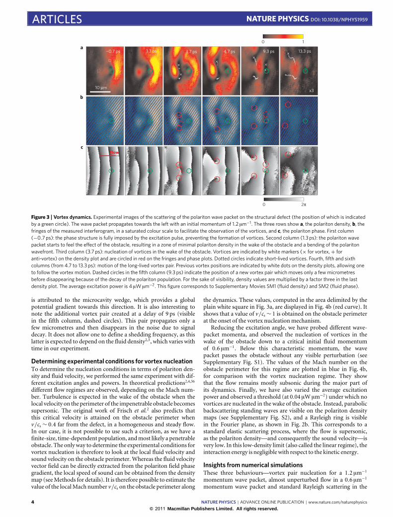
low-density flow—are extremely well reproduced by the numericalsimulations (see Supplementary Figs S3, S4, S5), which takeinto account the pulsed excitation, the finite spot size and theexponential decay of the polariton population (see Methods). Asnapshot of the computed phase profile is displayed in Fig. 5a,for the vortex nucleation regime, at the onset of the first vortexpair nucleation. Local values of the Mach number are representedby coloured lines, with a thick green line for v/cs = 1. Tocompare the experimental findings of Fig. 4b, we plot in Fig. 5bthe time evolution of the Mach number in a small region closeto the equator of the obstacle (small black and white circle inFig. 5a), using simulation parameters corresponding to the threeflow regimes described previously (vortex nucleation regime, low-velocity regime and low-density regime). Whereas the low-densityexperiment always lies in the supersonic region (black curve), thehigh-density experiments (blue and red curves) remain subsonic fora significant part of their dynamics. Similarly to the experimentalfindings, the low-velocity regime (blue curve) remains subsonicfor a longer time than the vortex nucleation regime (red curve).Moreover, consistently with the argument originally developed byFrisch et al.2 for the transition to turbulence in a superfluid, wefind in the simulation that the phase accumulation resulting invortex nucleation starts at the precise time when the fluid velocitybecomes equal to the sound speed (when v/cs= 1) on the obstacleequator. The nucleation of the vortex pair is just after this event;the higher the initial velocity, the closer the vortex nucleation

1

10

12840

Time (ps)

Low-density regime(supersonic)

Vortex nucleationregime

Low-velocityregime

a

b

2 µm

Mac

h nu

mbe

r v/

c s

Figure 5 | Nucleation criterion: numerical evidence. a, Numericalsimulation (see Methods for details) of the phase profile, with simulationparameters corresponding to the vortex nucleation regime at the onset ofvortex nucleation. The obstacle is indicated by a black circle and the flow isdirected to the left. The thick red circles show the vortex positions.Coloured lines indicate lines of equal Mach number. The thick green lineindicates a local Mach number of 1, blue lines indicate a local subsonic flow(v/cs < 1), yellow to red lines indicate a local supersonic flow (v/cs > 1).b, Evolution of the Mach number at the equator of the obstacle (small blackand white circle of Fig. 5a), using simulation parameters corresponding tothe vortex nucleation regime (red curve), to the low-velocity—mainlysubsonic—regime (blue curve) and to the low-density—linear—regime(black curve). The phase accumulation starts when the fluid velocitycrosses the sound velocity (v/cs= 1) on the obstacle equator (dashedlines) resulting in the systematic nucleation of vortices.

to the initial phase accumulation. The vortices are dragged awayfrom the obstacle at later times, in a time range correspondingto the experimental findings. Finally, the numerical simulationsallow one to see the role of the polaritonic nonlinearities in thenucleation process. Indeed, there are no vortices nucleated in thewake of the obstacle if the interaction constant is set to 0. Thehydrodynamic nucleation process can therefore be differentiatedfrom linear optical processes, such as the generation of vortexlattices, whenever three ormore plane waves interfere.

ConclusionOur experiment demonstrates the great potential of semiconductormicrocavities for the study of turbulence in quantum gases. The keyadvantages are the direct optical access to the polariton field (in bothreal and momentum spaces), the absence of a trapping potentialand operation at cryogenic temperature (and possibly even at roomtemperature in state-of-the-art nitride-based microcavities37). Theability to control polariton properties opens the way to subsequentbreakthrough experiments, such as the scattering of a wave packeton engineered obstacles of different sizes and shapes38,39, which

NATURE PHYSICS | ADVANCE ONLINE PUBLICATION | www.nature.com/naturephysics 5© 2011 Macmillan Publishers Limited. All rights reserved.

ARTICLES NATURE PHYSICS DOI: 10.1038/NPHYS1959

would provide the possibility to address the quantum counterpartof Bénard–VonKármán vortex streets and fully turbulent regimes7.

MethodsSample. The sample is a GaAs λmicrocavity sandwiched between two distributedBragg reflectors (DBR) with 22 (21) AlAs/GaAs pairs for the bottom (top) DBR,and one 8 nm thick InGaAs QW placed at the anti-node of the cavity field. It isheld in a cold finger cryostat at liquid helium temperature. We measured a Rabisplitting of 3.5meV and a cavity mode quality factor of Q= 7×103. The obstacleconsists of a structural defect in the microcavity plane. It is most likely penetrable.Its characteristic size can be estimated from Supplementary Fig. S1 to be 2 µm in thedirection of the flow and 5 µm in the direction transverse to the flow.

Experimental set-up. The polariton population is created using a pulsedTi:sapphire laser. The circularly polarized laser pulse is spectrally filtered to forma 1meV broad, 3 ps long pulse, which is then split into one excitation pulseand one reference pulse. The reference pulse is directed through a telescopefor spatial filtering and wavefront tuning, and incident at a slight angle on theCCD, to serve as a phase reference40. The excitation pulse is passed througha delay line and focused on the back of the sample using a 25 cm focal lengthcamera objective, providing a Fourier limited 25 µm diameter excitation spot. Anoblique excitation angle is used to create a propagating polariton wave packet.The coherent emission is collected by means of a 0.5 NA microscope objective ina transmission configuration. Real space or Fourier space images of the coherentemission are allowed to interfere, in a Mach–Zehnder configuration, with thereference pulse on the CCD. From the interferogram we numerically extract theamplitude and phase of the coherent emission at a time given by the delay betweenthe excitation and reference pulses. Varying this delay allows us to probe thedynamics of the coherent polariton population in both real and momentum spaces.By acquiring data over 0.2 s, every measurement is an integration over 1.6×107experimental realizations.

Numerical extraction of polariton amplitude and phase. To extract the polaritonamplitude and phase from the recorded interferogram, we use a technique knownas digital off-axis holography41. It consists of performing a two-dimensional fastFourier transform (FFT) of the interferogram. The fringes of the interferogramprovide off-axis contributions in the Fourier plane, which can be differentiatedfrom the cw contributions. Removing the cw contributions and performing aninverse FFT allows one to isolate the fringes, from which the amplitude andphase are extracted, providing the full information (amplitude and phase) on thecoherent polariton field.

Extraction of local fluid velocity and speed of sound from experimental data.The fluid velocity vector field is extracted from the phase gradient of the polaritonfield. The values of Fig. 4a are obtained by fitting the slope of the phase profile inthe region of interest. The error bars take into account the standard deviation of thelinear fit, as well as a systematic error coming from the determination of the phasegradient induced by the set-up alignment (see ref. 40 for how this reference phasegradient can be determined). The value of the local sound velocity is determinedfrom the density map, originally in arbitrary units, which needs to be scaled tothe blue-shift ng . We have access only to the spatially and temporally averagedblue-shift in the polariton dispersion, which is measured to be 0.8meV. Assumingthat the major contribution to this blue-shift comes from the beginning of thedynamics, when the maximal population density is reached, we scale the densitymaps to the blue-shift. This allows us to extract a rough estimation for the localspeed of sound along the dynamics (it more probably gives a lower bound to itsvalue, as the averaging of the blue-shift yields an underestimation of its value). Weconsider an error in the local sound velocity which takes into account the standarddeviation on the averaging in the region of interest, as well as a systematic error onthe scaling method, estimated to 25%.

Gross–Pitaevskii equation. We theoretically investigate the quantum turbulenceregime of exciton-polaritons in the mean field approximation. We solveiteratively the generalized Gross–Pitaevskii equation for the lower polariton modeψ , previously introduced byCiuti andCarusotto for exciton polaritons34

ihddtψ(r,t ) =

(−iγ

2+

∑k

hωk |k〉〈k|+g |ψ(r,t )|2)ψ(r,t )

+Vψ(r,t )+Fk(r,t )

The potential V is constructed as a 3 µm sized and 1meV high obstacle. Ourmodel accounts for the dissipation of polaritons, at rate γ , and a 1 ps-long initialexcitation of the system Fk(r,t ). The polariton–polariton interaction is assumed todepend linearly on the polariton density |ψ(r,t )|2 with a coefficient g . The lowerpolariton dispersion is approximated to a quadratic dispersion with effective massmLP. The parameters used in the simulations are: γ = h/15 ps, g = 0.01meV µm2,

hωk = h2k2‖/2mLP with mLP = 0.7meVps2 µm−2. The excitation intensity for

the high excitation experiment corresponds to a maximal polariton density of120 µm−2 on a 20 µm large spot.

Received 3 November 2010; accepted 28 February 2011;published online 3 April 2011

References1. Bergé, P., Pomeau, Y. & Vidal, C. Order Within Chaos: Towards a Deterministic

Approach to Turbulence (Wiley, 1986).2. Frisch, T. et al. Transition to dissipation in a model superflow. Phys. Rev. Lett.

69, 1644–1647 (1992).3. Winiecki, T., McCann, J. F. & Adams, C. S. Pressure drag in linear and

nonlinear quantum fluids. Phys. Rev. Lett. 82, 5186–5189 (1999).4. Winiecki, T. et al. Vortex shedding and drag in dilute Bose–Einstein

condensates. J. Phys. B 33, 4069–4078 (2000).5. Barenghi, C. F., Donnelly, R. J. & Vinen,W. F. (eds)Quantized Vortex Dynamics

and Superfluid Turbulence (Springer, 2001).6. Aftalion, A. et al. Dissipative flow and vortex shedding in the Painlevé boundary

layer of a Bose–Einstein condensate. Phys. Rev. Lett. 91, 090407 (2003).7. Sasaki, K. et al. Bénard–von Kármán vortex street in a Bose–Einstein

condensate. Phys. Rev. Lett. 104, 150404 (2010).8. Mironov, V. A. et al. Structure of vortex shedding past potential barriersmoving

in a Bose–Einstein Condensate. J. Exp. Theor. Phys. 110, 877–889 (2010).9. Raman, C. et al. Evidence for a critical velocity in a Bose–Einstein condensed

gas. Phys. Rev. Lett. 83, 2502–2505 (1999).10. Onofrio, R. et al. Observation of superfluid flow in a Bose–Einstein condensed

gas. Phys. Rev. Lett. 85, 2228–2231 (2000).11. Madison, K. W., Chevy, F., Wohlleben, W. & Dalibard, J. Vortex formation in

a stirred Bose–Einstein condensate. Phys. Rev. Lett. 84, 806–809 (2000).12. Madison, K. W., Chevy, F., Bretin, V. & Dalibard, J. Stationary states of a

rotating Bose–Einstein condensate: Routes to vortex nucleation. Phys. Rev. Lett.86, 4443–4446 (2001).

13. Raman, C., Abo-Shaeer, J. R., Vogels, J. M., Xu, K. & Ketterle, W. Vortexnucleation in a stirred Bose–Einstein condensate. Phys. Rev. Lett. 87,210402 (2001).

14. Yarmchuk, E. J., Gordon, M. J. V. & Packard, R. E. Observation of stationaryvortex arrays in rotating superfluid helium. Phys. Rev. Lett. 43, 214–217 (1979).

15. Henn, E. A. L., Seman, J. A., Roati, G., Magalhes, K. M. F. & Bagnato, V. S.Emergence of turbulence in an oscillating Bose–Einstein condensate.Phys. Rev. Lett. 103, 045301 (2009).

16. Inouye, S. et al. Observation of vortex phase singularities in Bose–Einsteincondensates. Phys. Rev. Lett. 87, 080402 (2001).

17. Neely, T. W. et al. Observation of vortex dipoles in an oblate Bose–Einsteincondensate. Phys. Rev. Lett. 104, 160401 (2010).

18. Amo, A. et al. Superfluidity of polaritons in semiconductor microcavities.Nature Phys. 5, 805–810 (2009).

19. Weisbuch, C. et al. Observation of the coupled exciton-photon modesplitting in a semiconductor quantum microcavity. Phys. Rev. Lett. 69,3314–3317 (1992).

20. Cerna, R. et al. Coherent optical control of the wave function ofzero-dimensional exciton polaritons. Phys. Rev. B 80, 121309(R) (2009).

21. Nardin, G. et al. Selective photoexcitation of confined exciton-polaritonvortices. Phys. Rev. B 82, 073303 (2010).

22. Saba, M. et al. High-temperature ultrafast polariton parametric amplificationin semiconductor microcavities. Nature 414, 731–735 (2001).

23. Kasprzak, J. et al. Bose–Einstein condensation of exciton polaritons. Nature443, 409–414 (2006).

24. Carusotto, I. et al. Fermionized photons in an array of driven dissipativenonlinear cavities. Phys. Rev. Lett. 103, 033601 (2010).

25. Love, A. P. D. et al. Intrinsic decoherence mechanisms in the microcavitypolariton condensate. Phys. Rev. Lett. 101, 067404 (2008).

26. Lagoudakis, K. G. Coherent oscillations in an exciton-polariton Josephsonjunction. Phys. Rev. Lett. 105, 120403 (2010).

27. Wertz, E. et al. Spontaneous formation and optical manipulation of extendedpolariton condensates. Nature Phys. 6, 860–864 (2010).

28. Lagoudakis, K. G. et al. Quantized vortices in an exciton-polariton condensate.Nature Phys. 4, 706–710 (2008).

29. Lagoudakis, K. G. et al. Observation of half-quantum vortices in anexciton-polariton condensate. Science 326, 974–976 (2009).

30. Roumpos, G. et al. Single vortex–antivortex pair in an exciton-polaritoncondensate. Nature Phys. 7, 129–133 (2011).

31. Krizhanovskii, D. N. et al. Effect of interactions on vortices in a nonequilibriumpolariton condensate. Phys. Rev. Lett. 104, 126402 (2010).

32. Sanvitto, D. et al. Persistent currents and quantized vortices in a polaritonsuperfluid. Nature Phys. 6, 527–533 (2010).

33. Amo, A. et al. Collective fluid dynamics of a polariton condensate in asemiconductor microcavity. Nature 457, 291–295 (2009).

6 NATURE PHYSICS | ADVANCE ONLINE PUBLICATION | www.nature.com/naturephysics

© 2011 Macmillan Publishers Limited. All rights reserved.

NATURE PHYSICS DOI: 10.1038/NPHYS1959 ARTICLES34. Carusotto, I. et al. Probing microcavity polariton superfluidity through

resonant Rayleigh scattering. Phys. Rev. Lett. 93, 166401 (2010).35. Bolda, E. L. et al. Dissipative optical flow in a nonlinear Fabry–Perot cavity.

Phys. Rev. Lett. 86, 416–419 (2001).36. Pigeon, S. et al. Hydrodynamic nucleation of vortices and

solitons in a resonantly excited polariton superfluid. Preprint athttp://arxiv.org/abs/1006.4755 (2010).

37. Christmann, G. et al. Room temperature polariton lasing in a GaN/AlGaNmultiple quantum well microcavity. Appl. Phys. Lett. 93, 051102 (2008).

38. Kaitouni, R. I. et al. Engineering the spatial confinement of exciton polaritonsin semiconductors. Phys. Rev. B 74, 155311 (2006).

39. Amo, A. et al. Light engineering of the polariton landscape in semiconductormicrocavities. Phys. Rev. B 82, 081301(R) (2010).

40. Nardin, G. et al. Phase-resolved imaging of confined exciton-polariton wavefunctions in elliptical traps. Phys. Rev. B 82, 045304 (2010).

41. Kreis, T. Holographic Interferometry—Principles and Methods(Akademie, 1996).

AcknowledgementsWe would like to thank M. Wouters and T. C. H Liew for enlightening discussions. Weacknowledge support by the Swiss National Science Foundation through the ‘NCCRQuantum Photonics’.

Author contributionsG.N. and G.G performed the experiments. Y.L. performed the numerical simulations.F.M-G. grew the sample. G.N, Y.L and B.P. wrote the paper. B.D-P. supervised theproject. All authors contributed to numerous discussions and data analysis.

Additional informationThe authors declare no competing financial interests. Supplementary informationaccompanies this paper on www.nature.com/naturephysics. Reprints and permissionsinformation is available online at http://npg.nature.com/reprintsandpermissions.Correspondence and requests formaterials should be addressed to G.N.

NATURE PHYSICS | ADVANCE ONLINE PUBLICATION | www.nature.com/naturephysics 7© 2011 Macmillan Publishers Limited. All rights reserved.