Hydraulic Scilab toolbox for water distribution systems

powered by

EnginSoft SpA - Via della Stazione, 27 - 38123 Mattarello di Trento | P.I. e C.F. IT00599320223

A HYDRAULIC SCILAB TOOLBOX

FOR WATER DISTRIBUTION SYSTEMS

Authors: M. Venturin

Keywords: Hydraulic system; Scilab; Xcos; Xcos + Modelica

Abstract: The purpose of this paper is to show the possibilities offered by Scilab/Xcos to model hydraulic time-dependent systems. In particular, we develop a new Xcos module combined with the use of Modelica language to show how water distribution systems can be modeled and studied. In this paper we construct a reduced library composed by few elements: reservoirs, pipes and nodes. The library can be easily extended to obtain a more complete toolbox. The developed library is tested on a simple well-known hydraulic circuit.

Contacts [email protected]

This work is licensed under a Creative Commons Attribution-NonCommercial-NoDerivs 3.0 Unported License.

mailto:[email protected]

A hydraulic system toolbox

www.openeering.com page 2/17

1. Introduction

Studying water distribution systems (WDS) is very important for a correct supply of water. These studies can guarantee an adequate water pressure at each location of frequent use and can reduce the total costs of water distribution systems.

Studying of water distribution systems requires a simulation tool that can be based on the following (at least) elements that are the basic building blocks of any network:

1. Pipes;

2. Node or junctions;

3. Storage tanks and reservoirs.

Moreover, the developed library can be straightforward extended with other elements like pumps and valves that are typically found in a hydraulic network.

Solving the network problem consists of finding the flow of water in each pipe and pressure level at each node. The required input data are:

1. The network layout;

2. The governing equations which describe the physics of the system;

3. The consumer’s demand;

Here, in this work, we consider only the numerical modeling of the hydraulic part. The library is developed in Scilab/Xcos with the use of Modelica features. For more real-case applications the interested reader can contact the Openeering team.

Typically, the WDS problem is often associated to a multiobjective optimization problem where we want to maximize the minimum of the pressure level at nodes and minimize the total cost of the entire network. For optimizing the network we need to couple the hydraulics simulator with an appropriate multiobjective optimization tool. In Scilab, this can be done in a unified language since the hydraulic part can be modeled in Xcos/Modelica while the optimization part can be done using the available multiobjective optimization toolbox.

The paper is organized as follows. First we presented the basic modeling strategy, then the constitutive laws of the network elements and finally we presented an application of the developed library to simulate a simple hydraulic circuit. Comparison results are done with respect to the Epanet [1] software.



2. The problem description

In this tutorial we analyze the distribution network shown in Figure 1. It consists of 8 pipes, 6 junction nodes at different levels and one reservoir.

Figure 1: Network layout.

This model can be used as an example of water distribution systems where it is possible to detect negative value for the pressure. These negative values indicate situations where there is a deficit of pressure and this should be avoid in real situations. Finding the best combination of pipes can be easily done with our model if we couple it with an optimization algorithm. An example of this process is done in [2].

Figure 2: Actual piezometric line and pressure levels



The characteristics of the nodes are shown in Table 1 where we report elevation and customer’s demand at each node.

Table 1: Nodes data

Node Demand (m^3/h) Elevation (ft)

1 --- 210

2 100 150

3 100 160

4 120 155

5 270 150

6 330 165

7 200 160

Pipes properties are reported in Table 2.

Table 2: Pipes data

Pipe Length (ft) Diameter (in)

1 1000 18

2 1000 10

3 1000 16

4 1000 4

5 1000 16

6 1000 10

7 1000 10

8 1000 1



3. Library modeling

In this section we describe the basic library modeling approach. The Modelica developed package is named “WDS” (Water Distribution System) and it is contained in the file “WDS.mo”. In this file we develop the library in the Modelica language 2.0 where the balance between equations and variables is not required for any local element.

A version of the file, using Modelica language 3.0, can be found in the file “WDS_new.mo” and it is described in Appendix A.

The implementation of the toolbox is done in Scilab/Xcos through the use Modelica features. The first step is to identify through and across system variables and the use of the “passive sign convention1” for all elements.

For our problem we choose:

the volumetric flow rate [GPM] as the through variable;

the total head [ft] as an across variable.

the elevation [ft] as an across variable.

Hence, our modeling is characterized by one through variable and two across variables.

This is implemented in the connector class named “Pin”:

connector Pin "Inlet port"

Real H "Total head [ft]";

flow Real q "Volumetric flow [GPM]";

Real z "Elevation [ft]";

end Pin;

The previous class implements the basic conservation laws for a two pins element:

Flux of the element = Flux element at the input node

= - Flux element at the output node

and

Head drop = Head at the input node

- Head at the output node

and

Delta Elevation = Elevation at the input node

– Elevation at the output node

1 In the “user convention” the through variable enters the positive terminal of a component (in Scilab is denoted by the black square).



4. Element constitutive laws and properties

In this section we summarize the constitutive laws and properties that have been used to develop the toolbox.

4.1. Some constants

Here we report some constants that are used in the development of the constitutive laws of the elements available in the library. Here we list the constants we use:

is the number;

is the minimum time used in the definition of the junction element;

is the specific gravity or relative density that is the ratio between the substance density and the density of water at 4° [C];

is the conversion pressure factor;

is the unit conversion factor used in the hydraulic pipe element;

is the conversion of 1 [ft3/s] to 1 [US gallon per minute];

.is the minimum value used in the modeling of the hydraulic resistance element.

The library constants are defined as follows:

package Constants "Simulation library constants"

constant Real pi = 3.14159265358979323846 "pi";

constant Real tmin = 1 "Minimum simulation time for linearization [s]";

constant Real SG = 1 "Specific gravity";

constant Real pheadconst = 2.3041475 "Unit conversion";

constant Real k = 1.318 "Unit conversion";

constant Real Qconv = 448.8312 "Unit conversion";

constant Real Qmin = 1e-8 "Minimum flow [ft^3/s]";

end Constants;

4.2. Reservoir elements

The equations of a generic reservoir element fix the total head and the elevation given the user input specification , i.e.

The total head equation: [ft];

The elevation equation: [ft];

The Modelica implementation is done in the class “Reservoir”:

model Reservoir

Pin Outlet;

parameter Real Zval = 210. "Elevation [ft]";

equation

Outlet.H = Zval "Total head";

Outlet.z = Zval "Elevation";

end Reservoir;



4.3. Junction elements

A junction of a node is an element where it is possible to specify elevation and customer’s demand .

The element is composed of the following two equations:

The elevation equation that fixes the elevation [ft];

The flux equation that fixes the customer’s demand [GPM].

In our implementation the load (customer’s demand) is modeled in a time dependent manner such that the customer’s demand is reached after the time . There is a transition zone in which the initial load is zero; this guarantees that at the initial time everything is in equilibrium.

The level pressure is obtained from the equation (conversion from head feet to pressure in psi):

where:

is the pressure level [psi];

is the conversion factor;

is the specific gravity or relative density [-];

is the node head [ft]

is the node element total head [ft];

is the node elevation [ft];

The Modelica implementation is done in the class “Junction”:

model Junction

Pin Inlet;

parameter Real Zval = 150. "Elevation [ft]";

parameter Real Qval = 100. "Base Demand [GPM]";

Real Pressure "Pressure [psi]";

Real Qflux "Current time base demand [GPM]";

protected

constant Real tmin = WDS.Constants.tmin;

constant Real SG = WDS.Constants.SG;

constant Real pheadconst = WDS.Constants.pheadconst;

equation

Qflux = if time<tmin then (Qval/tmin)*time else Qval "Current flux";

Inlet.q = Qflux "Flux at the inlet";

Inlet.z = Zval "Elevation";

Pressure = (Inlet.H - Zval) * SG / pheadconst "Pressure head";

end Junction;



4.4. Hydraulic pipe

Hydraulic resistor in pipe is modeled using the Hazen-William friction loss equation:

where:

is the discharge [ft3/s];

is the energy slope [ft/ft];

is the hydraulic radius [ft];

is the fluid velocity [ft/s];

is the hydraulic diameter [ft];

is the pipe length [ft];

is the energy head loss [ft];

is the H-W coefficient [-]

is the unit conversion factor.

This equation relates and . As a note, a linear version of the equation is used if the flow is

under a pre-fixed flow tolerance .

The Modelica implementation is done in the class “Pipe”:

model Pipe

Pin Inlet;

Pin Outlet;

parameter Real Lval = 1000. "Pipe length [ft]";

parameter Real Dval = 12. "Pipe diameter [in]";

parameter Real Cval = 130. "Hazen-Williams coefficient [-]";

Real q "Fluid through the element [GPM]";

Real Dh "Hydraulic diameter [ft]";

Real Rh "Hydraulic radius [ft]";

Real A "Area [ft^2]";

Real Qdisc "Discharge [ft^3/s]";

Real v "Velocity [ft/s]";

Real S "Energy slope [ft/ft]";

Real hf "Energy loss [ft]";

// - Linearize version due to numerical derivative problems

Real vmin "Minimum velocity [ft/s]";

Real Smin "Minimum energy slope [ft/ft]";

Real hfmin "Minimum energy loss [ft]";

protected

constant Real pi = WDS.Constants.pi;

constant Real k = WDS.Constants.k;

constant Real Qconv = WDS.Constants.Qconv;

constant Real Qmin = WDS.Constants.Qmin;

equation

Inlet.q = q "Flux inlet";

Outlet.q = -q "Flux outlet";

Dh = Dval / 12. "Hydraulic diameter [ft]";



Rh = Dh / 4. "Hydraulic radius [ft]";

A = pi * Dh^2 / 4. "Area [ft^2]";

Qdisc = q / Qconv "Discharge [ft^3/s]";

v = abs(Qdisc) / A "Velocity [ft^3/s]";

S = (v/(k*Cval*Rh^0.63))^(1./0.54) "Energy slope [ft/ft]";

hf = sign(Qdisc) * S * Lval "Energy loss [ft]";

// Evaluate linearize version

vmin = Qmin / A;

Smin = (vmin/(k*Cval*Rh^0.63))^(1./0.54);

hfmin = Smin * Lval;

// Inlet.H - Outlet.H = hf "Pressure head"; // Not a good choice in

numerical analysis

Inlet.H - Outlet.H = if abs(Qdisc) < Qmin then hfmin*(Qdisc/Qmin) else

hf "Pressure head";

end Pipe;



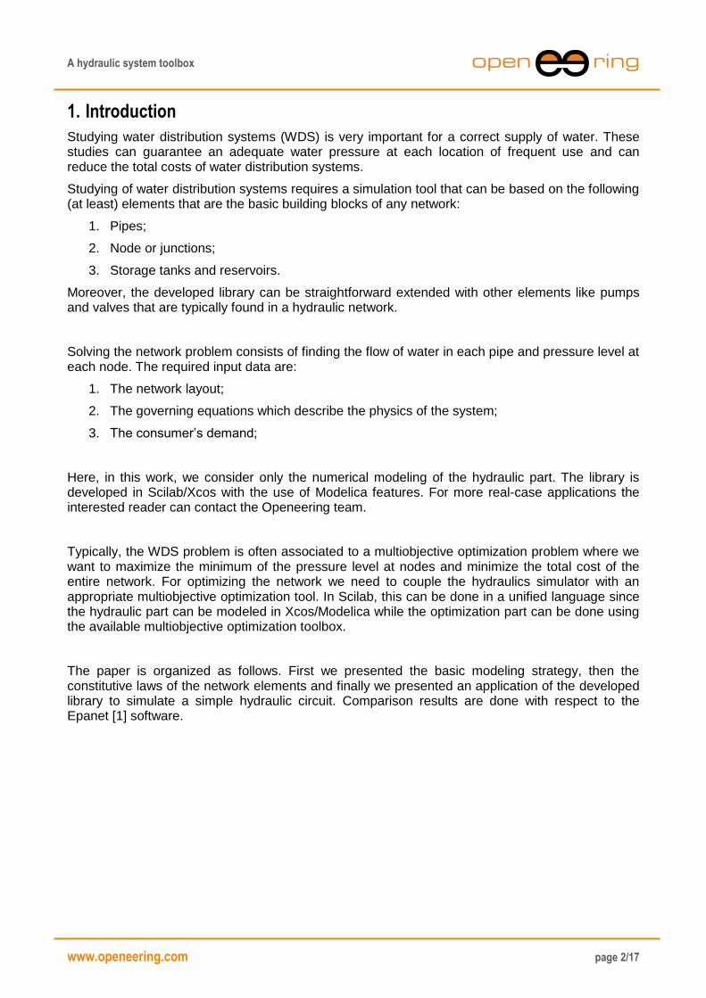
5. Example

The Xcos scheme of the problem is reported in Figure 3. See the Appendix B for the element specifications.

Figure 3: The simulation network.

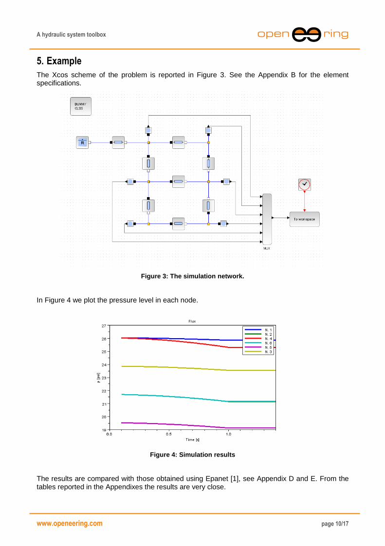
In Figure 4 we plot the pressure level in each node.

Figure 4: Simulation results

The results are compared with those obtained using Epanet [1], see Appendix D and E. From the tables reported in the Appendixes the results are very close.



6. Conclusion

Here, we have developed a Scilab/Xcos toolbox for hydraulic simulation. The toolbox will be extended in the future by providing further elements. For more real-case applications the interested reader can contact the Openeering team.

7. References

[1] Epanet software and user manual, http://www.epa.gov/nrmrl/wswrd/dw/epanet.html.

[2] Matteo Nicolini: A Two-Level Evolutionary Approach to Multi-criterion Optimization of Water Supply Systems. Evolutionary Multi-Criterion Optimization, Third International Conference, EMO 2005, Guanajuato, Mexico, March 9-11, 2005, Proceedings: 736-751

http://www.epa.gov/nrmrl/wswrd/dw/epanet.html



Appendix A – Library in new Modelica style

The connector





end Pin;

is not a valid connector since the number of flow variables and the number of non-flow variables do not correspond. In new Modelica style it is required that the number of flow variables in a connector is equal to the number of non-causal, non-flow variables (variables without prefix flow, input, output, stream, parameter and constant) in order to guarantee that the model has balanced equations.

Here, we propose a simple solution by introducing a support flow variable (dummy). The definition of the new connector becomes:





flow Real dummy;

end Pin;

Then, it is only necessary to modify the element “Pipe” by introducing the following equations:

// dummy part

Inlet.dummy = 0 "Flux inlet";

Outlet.dummy = 0 "Flux outlet";

A more correct approach should be based on stream and input/output connectors but this is beyond the scope of this tutorial.



Appendix B – Library description

In the following table we report all the developed elements of our water distribution system (WDS) library.

Element Required parameters Xcos element

Junction

Pipe

Reservoir



Appendix C – Software installation and testing

The “hydraulic system toolbox” is available to registered users only. For downloading the library visit:

http://www.openeering.com/registered_users_area

Registration is free and automatic.

To load the library into the Xcos environment type

--> exec loader.sce

from the main directory. The new set of palette is loaded in your Xcos system.

Figure 5: The Aeraulic library in Xcos

Open the Xcos model file " Example_HydraulicNet.xcos" and run it. Remember that to run an

Xcos model with Modelica blocks, a C compiler should be installed in your system. Check if a

compiler is available in your system with the Scilab command "haveacompiler()".

Then analysis of the data is done using the function "Example_ProcessData.sce", the plot can

be generated using the function "Example_PlotData.sce".

The directory “other” contains the Epanet example and the Modelica libraries used to produce this article.

http://www.openeering.com/registered_users_area



Appendix D – Epanet results

In the following we report the results obtained using Epanet software [1].

Page 1 03/05/2012 15.17.54

**********************************************************************

* E P A N E T *

* Hydraulic and Water Quality *

* Analysis for Pipe Networks *

* Version 2.0 *

**********************************************************************

Input File: Example_HydraulicNet.net

Link - Node Table:

----------------------------------------------------------------------

Link Start End Length Diameter

ID Node Node ft in

----------------------------------------------------------------------

1 1 2 1000 18

2 2 3 1000 10

3 2 4 1000 16

4 4 5 1000 4

5 4 6 1000 16

6 6 7 1000 10

7 3 5 1000 10

8 7 5 1000 1

Node Results:

----------------------------------------------------------------------

Node Demand Head Pressure Quality

ID GPM ft psi

----------------------------------------------------------------------

2 100.00 209.57 25.81 0.00

3 100.00 208.74 21.12 0.00

4 120.00 209.26 23.51 0.00

5 270.00 208.32 25.27 0.00

6 330.00 209.06 19.09 0.00

7 200.00 208.75 21.12 0.00

1 -1120.00 210.00 0.00 0.00 Reservoir



Link Results:

----------------------------------------------------------------------

Link Flow VelocityUnit Headloss Status

ID GPM fps ft/Kft

----------------------------------------------------------------------

1 1120.00 1.41 0.43 Open

2 336.88 1.38 0.82 Open

3 683.12 1.09 0.31 Open

4 32.56 0.83 0.94 Open

5 530.56 0.85 0.19 Open

6 200.56 0.82 0.31 Open

7 236.88 0.97 0.43 Open

8 0.56 0.23 0.43 Open



Appendix E – Simulation results

Here, we report the simulation results obtained using our modeling approach.

------------------------------------------------------

Link Start End Length Diam. H-Z

ID node node Const.

------------------------------------------------------

1 1 2 1000 18 130

2 2 3 1000 10 130

3 2 4 1000 16 130

4 4 5 1000 4 130

5 4 6 1000 16 130

6 6 7 1000 10 130

7 3 5 1000 10 130

8 7 5 1000 1 130

------------------------------------------------------

-------------------------------------------

Link Flow Velocity Headloss

-------------------------------------------

1 1120.00000 1.41209 0.43422

2 336.87830 1.37614 0.82184

3 683.12160 1.09005 0.30847

4 32.56250 0.83136 0.94130

5 530.55910 0.84661 0.19317

6 200.55920 0.81928 0.31455

7 236.87840 0.96764 0.42811

8 0.55916 0.22842 0.43364

-------------------------------------------

-------------------------------------------------

NODE Demand Head pressure

-------------------------------------------------

1 -1120.00000 210.00000 0.00000

2 100.00000 209.56578 25.85155

3 100.00000 208.74394 21.15487

4 120.00000 209.25731 23.54767

5 270.00000 208.31601 25.30915

6 330.00000 209.06414 19.12383

7 200.00000 208.74965 21.15735

-------------------------------------------------

Hydraulic Scilab toolbox for water distribution systems

Engineering

Transcript of Hydraulic Scilab toolbox for water distribution systems