Hydraulic performance of biofilter systems for stormwater management: lessons from a field study

Sébastien Le Coustumer, Tim D. Fletcher Ana Deletic & Matthew Potter

Facility for Advancing Water Biofiltration, Department of Civil Engineering, Institute

for Sustainable Water Resources, Monash University, Melbourne, Vic., 3800, Australia

Supported by the Better Bays and Waterways Institutionalising Water Sensitive Urban Design and Best Management Practice in Greater Melbourne Project, Melbourne

Water, East Melbourne, 3002, Australia.

2

This study was undertaken under the Facility for Advancing Water Biofiltration, as part of PROJECT 4: DEMONSTRATION AND TESTING (ACTIVITY 4.03: Investigation into the long term sustainability of stormwater bioretention systems). It was supported by funding through the Better Bays and Waterways - Institutionalising Water Sensitive Urban Design and Best Practice Management in greater Melbourne project. Funding partners are the Australian Government through the Coastal Catchment Initiative funded through the Natural Heritage Trust, Department of Sustainability and Environment, Melbourne Water, Clearwater and the City of Kingston. April 2008 Contact details: Sebastien.le.coustumer@eng.monash.edu.au Tim.fletcher@eng.monash.edu.au Ana.deletic@eng.monash.edu.au matthew.potter@melbournewater.com.au

3

Executive summary

Biofiltration systems (‘biofilters’) are increasingly being used to manage

polluted stormwater runoff in urban areas. However, there are significant concerns

about their lifespan, particularly due to the possibility of clogging of the systems over

time. A study of 37 biofilters constructed on the east coast of Australia during the last

seven years, shows that 60% of constructed systems have a saturated hydraulic

conductivity (K) which meets or exceeds the currently recommended range of 50 to 200

mm/h. It appears that the media used varied greatly between systems, perhaps because

of a lack of available guidelines at the time of construction, or because of inadequate

specification and quality control. However, this generally does not affect the treatment

efficiency of the systems, as most systems surveyed were sufficiently sized (in filter

area or ponding volume) such that their detention storage volume compensates for

reduced media hydraulic conductivity (Figure 1). Consideration of the interaction

between these three design elements – hydraulic conductivity, filter area and detention

(ponding depth) – is critical (rather than consideration of one factor in isolation).

filter media hydraulic

conductivity conductivity

extended detention

depth

filter surface

area

infiltration capacity

Figure 1. Interaction between media hydraulic conductivity and other design components, in

determining infiltration capacity of the bioretention system.

The study broadly reveals two types of systems: some with a high initial K

(>200 mm/h) and some with a low initial K (<20 mm/h). Significant reductions in K are

evident for biofilters in the former group, although most are shown to maintain an

acceptably high conductivity. For the second type of systems (with low initial K), little

4

change occurs over time. Two hypotheses could explain this phenomenon: on one hand

sediment depositions could be leading to the clogging of the surface of the system;

another possibility is that the creation of macropores through root growth and dieback

may help to minimise the reduction in K. The impact of surface clogging is

proportionally greater in systems which started with a high initial K, most likely

because the difference in particle size distribution between the original filter media and

deposited sediments will be greater where the original media was coarse. In the systems

with low initial K, the finer particle size distribution will be more similar to that of the

inflow sediments (although still considerably larger), thus reducing the proportional

impact of any surface clogging effect.

Site characteristics such as filter area as a proportion of catchment area, age of

the system and inflow volume were not found to be useful predictors of media

conductivity, with initial conductivity of the original media explaining the vast majority

of variance. It is clear therefore, that strict attention must be paid to the specification of

original filter media, to ensure that it satisfies current design requirements. Media

should be tested after construction of the system.

Given the apparent difficult in specifying and maintaining hydraulic conductivity

in biofiltration media, one approach is to use a “contingency factor” in the specification

of hydraulic conductivity for biofiltration systems. For example, where the design

intent is to use a soil media with a hydraulic conductivity of 180 mm/hr, sizing of the

system should be undertaken assuming a hydraulic conductivity of 50% of the design

value (ie. 90 mm/hr). In this way, if the media does not meet specifications, or shows a

decline in hydraulic conductivity over time, the overall system performance will remain

satisfactory.

Key words: Biofilters, clogging, stormwater management, hydraulic conductivity

5

Table of contents

1 Introduction .............................................................................................................. 6 2 Method...................................................................................................................... 9

2.1 Sampling locations ........................................................................................... 9

2.2 Sampling methodology..................................................................................... 9

Single ring field infiltration test (shallow test) ....................................................... 10

Deep ring field infiltration test ................................................................................ 11

Laboratory infiltration test...................................................................................... 12

Limitations of the sampling methods...................................................................... 12

2.3 Data analysis................................................................................................... 13

3 Results and discussion............................................................................................ 15

3.1 Biofilter design ............................................................................................... 15

3.2 Comparing field methods ............................................................................... 18

3.3 Comparing field and laboratory methods ....................................................... 19

3.4 Clogging of systems over time ....................................................................... 20

3.5 Influence of system characteristics and hydraulic performance..................... 23

4 Conclusions ............................................................................................................ 25 5 Acknowledgments .................................................................................................. 26 6 References .............................................................................................................. 27

6

1 Introduction

Biofiltration systems (also called bioretention systems, biofilters or rain gardens)

have been widely implemented in the last few years as a source control technique to

manage stormwater runoff in urban areas (Melbourne Water, 2005). They form one

technique in the suite of tools which aim to reduce the impact of urbanisation on

watersheds (Dietz and Clausen, 2007).

In Australia, they are commonly used to treat runoff in urbanizing areas and as a

retrofit technique in already-developed areas. With increasing societal pressure to

protect and restore the environmental quality of aquatic ecosystem (Brown and Clarke,

2007), local water authorities are encouraging their development and construction.

Biofilters have been shown to be effective in the treatment of suspended

sediments, heavy metals and nutrients (Zinger et al. 2007). However, there remain

significant questions about the sustainability and long-term performance of biofilters,

with little field data available.

Australian guidelines for biofilter design generally recommend a saturated

hydraulic conductivity (K) of between 50 and 200 mm/h for the filter media (e.g.

Melbourne Water, 2005). Biofilters are then designed in order to achieve pollutant

removal efficiency for total suspended solids (TSS), total nitrogen (TN) and total

phosphorus (TP), as described in Table 1. Curves giving the percentage of pollutant

removal versus the size of biofilter for different detention depth have been developed, to

determine required area and detention volume (Melbourne Water, 2005). As an

example, in the Melbourne area, if a 300 mm detention depth is assumed, a biofilter has

to be sized at approximately 1.65% of the impervious catchment in order to achieve a 45

% TN removal (the limiting performance target required by regulations in several

Australian states).

Table 1: Quality objectives for stormwater treatment in Victoria (Victoria stormwater committee, 1999)

Pollutants Objective

TSS 80% retention of annual loading

TP 45% retention of annual loading

TN 45% retention of annual loading

7

The potential for clogging of the surface of the systems is a real issue (Bouwer,

2002). A field survey of a number of infiltration systems (which unfortunately did not

include raingardens or any other form of biofilters) conducted by Lindsey et al. (1992)

showed that only 38% of infiltration basins were functioning as designed after 4 years

of operation, with 31% considered to be clogged. Schueler et al. (1992) showed that

50% of infiltration systems were not working due to clogging. Clogging results in more

frequent overflows and therefore a decrease in treatment capacity, since less of the

annual flow volume filters through the media. Clogging may also cause problems of

stagnant water and aesthetic problems, leading to difficulties in acceptance of

biofiltration as a system integrated into the built environment.

To illustrate the impact of the variation of K on the performance of the system, the

Model for Urban Stormwater Improvement Conceptualisation (MUSIC v3.02) software

was used to model a hypothetical catchment of 1 ha (100% impervious) located in

Melbourne, draining into a biofilter designed at 1% of the catchment area, and with a

ponding depth of 10 cm. As shown in Figure 1, the percentage of mean annual flow

treated (called ‘hydrologic effectiveness’; Wong et al. 1999) decreases with K. For a K

of 200 mm/h, the hydrologic effectiveness is 85%; falling to 58% for K of 50 mm/h and

to 29% for K of 5 mm/h. When biofilters are severely clogged (for example when K is 5

mm/h), 71% of inflows are discharged effectively untreated to receiving waters.

0

10

20

30

40

50

60

70

80

90

100

1 10 100 1000Hydraulic conductivity (mm/h)

Rem

oval

of T

N lo

ad /

Hyd

rolo

gica

l Effe

ctiv

enes

s [%

of

annu

al in

flow

s]

Hydrological effectiveness

TN reduction

Figure 1 : Evolution of Hydrological effectiveness and TN reduction vs. Hydraulic conductivity

8

In this context, the objectives of this study are to:

Evaluate the hydraulic conductivity and the design of a large number of

systems already built in order to assess their performance regarding current

guidelines,

Assess the evolution of hydraulic conductivity in order to estimate the

variation of their performance with time,

Gather a large dataset on different systems in order to understand the

possible influence of some factors (i.e. catchment size, biofilter size, age…)

on their performance.

Provide guidance on the design and construction of rain-gardens, based on

findings of the survey.

9

2 Method

2.1 Sampling locations

Thirty-seven biofilters were sampled over 18 sites, in Melbourne, Sydney and

Brisbane. Measurements were taken in order to represent as well as possible any spatial

variability in hydraulic conductivity. Usually three measurements were taken in each

biofilter, most of the biofilters tested being less than 40 m² in area (Table 2).

The sites were deliberately chosen to have different characteristics. Impervious

catchment and biofilter size were measured for each. The distributions of the main

characteristics of the sites (catchment location, type and size, and biofilter size) are

presented in Table 2. The volume of water, the volume of water received by the system

every year and the total volume of water per m² of biofilter were calculated with the

following hypotheses: an average annual precipitation (Bureau of Meteorology):

Melbourne: 650 mm/h

Brisbane: 1200 mm/h

Sydney: 1175 mm/h

An annual runoff coefficient of 0.8 (to account for initial losses, etc).

Table 2: Site characteristics

Location # of sites Catchment use # of sites Catchment size # of sites Biofilter size # of sites

Melbourne 30 Residential 18 < 100m² 6 < 40m² 31

Brisbane 4 Industrial 8 100–1000 m² 17 40–400 m² 4

Sydney 3 Parking 5 1000-10000 m² 9 > 400 m² 2

Highway 4 > 10 000 m² 1

Low traffic road 2

2.2 Sampling methodology

A number of alternative methods were used (for comparative purposes) for

determination of hydraulic conductivity. Field hydraulic conductivity (Kfs)

measurement of biofilters, have been conducted by two different methods (used for

cross-checking the measurements):

10

(1) a single ring shallow infiltrometer (referred to herein as Kfs shallow), and

(2) a deep ring infiltrometer (herein referred to as Kfs deep).

Laboratory measurements of hydraulic conductivity were also conducted on two

types of samples:

(1) surface samples (Klab surf), and

(2) samples taken from deep in the filter media (at a depth of approximately 150

mm below the surface - referred to as Klab deep ini)

Whilst the surface measurement reflects the current effective hydraulic

conductivity of the system, the deep sample provides an estimate of the initial hydraulic

conductivity of the media. Methods used for determining each of these measures are

described in more detail in subsequent sections.

Single ring field infiltration test (shallow test)

The single ring infiltrometer test has been widely described in the literature (see

Reynolds and Elrick, 1990, Youngs et al. 1993 for example) and thus only a brief

summary is given here. This method measures the hydraulic conductivity at the surface

of the soil (and thus is most appropriate when the hydraulic conductivity is controlled

by a limiting layer at the media surface).

The single ring infiltrometer consists of a small plastic ring, with a diameter of

100 mm that is driven 50 mm into the soil (Figure 2). It is a constant head test that is

conducted for two different pressure heads (50 mm and 150 mm). The experiment is

stopped when the infiltration rate is considered steady (i.e. when the volume poured per

time interval remains constant for at least 20 minutes).

In order to calculate Kfs, a ‘Gardner’s’ behaviour for the soil was assumed

(Gardner, 1958 in Youngs et al. 1993): h

fseKhK α=)( Eq. 1

Where K - the hydraulic conductivity, h - the negative pressure head and α - a soil pore

structure parameter.

11

Kfs is then found using the following analytical expression (for a steady flow)

(Reynolds and Elrick, 1990):

aGaGHKq m

fs πφ

π++= )1( Eq. 2

Where q - the steady infiltration velocity, a -the ring radius, H - the ponding depth, φm -

the matrix flux potential and G a shape factor estimated as:

184.0316.0 +=adG

Eq. 3

Where d - the depth of insertion of the ring, and a - the ring radius. G is considered to be

independent of soil hydraulic conductivity (i.e. Kfs and α) and ponding, if the ponding

depth is greater than 50 mm.

Figure 2: Sketch of a biofilter with the deep ring and the shallow ring

Deep ring field infiltration test

The deep ring method is based on the lysimetric method as explained in Daniel

(1989), and may be more appropriate if the limiting hydraulic conductivity is found

considerably below the surface. In order to measure the Kfs with this method it is

necessary to have a free-draining outflow drain from which the discharge can be

measured. Biofilters are built effectively as a lysimeter (i.e. with a drainage layer made

of gravel and perforated pipe, both of which have a flow capacity several orders of

magnitude higher than the overlying filter media), but it was not feasible to flood each

biofilter and measure the outflow in the drain. However, by inserting a ring down to the

drainage layer (Figure 2), it is then possible to apply Darcy’s law, assuming the

following hypotheses: flow through the soil is uni-directional (vertical); soil is

Transition and drainage layer

Media filter (L)

Constant ponding depth (H)Possible clogged layer

Deep test Shallow test

To the drainage system

Transition and drainage layer

Media filter (L)

Constant ponding depth (H)Possible clogged layer

Deep test Shallow test

To the drainage system

12

saturated, we can then assume that the wetting front is going down the drainage layer

and will be as thick as the soil layer and there will be no pressure in the drainage layer

(ie. free drainage is assumed).

Darcy’s law (Eq. 4) can be then used to calculate the hydraulic conductivity.

( )fsQLK

H L A=

+ Eq. 4

Where L - the length of the media filter, H - the ponding depth, Q - the infiltration flow

rate (i.e., added volume of water to keep a constant head divided by the time step) and A

the cross sectional area of the column.

The cylinder used had a 130 mm internal diameter and was driven up to the gravel

layer. This method is able to measure the hydraulic conductivity of the whole system,

and can thus account for a limiting layer anywhere in the media depth profile.

Laboratory infiltration test

Soil samples were tested according to the Australian standard AS 4419-2003.

Tests were undertaken on disturbed samples (by necessity). Surface samples (called lab-

surface) were taken in the first centimetre of the soil and deep samples between 10 and

15 cm. Surface samples were used to compare the field and the laboratory method. Deep

samples (called lab-deep) are assumed to represent ‘the initial hydraulic conductivity’

of the systems because soil has not been changed by sediment deposit (any fine

sediment deposited on the filter is assumed to be trapped within the first few

centimetres of the media (Hatt et al, 2006). The dimensions of samples tested during the

experiments were 100 mm diameter and 85 mm deep.

Limitations of the sampling methods

For both field tests, the main limitations are the possible compaction or

disturbance of the soil while the ring is driven into the soil and possible preferential

flow on the side of the column. For the deep ring method, it is also possible that the

assumptions of saturated conditions at the beginning of the experiment, and the free-

draining behaviour of the underlying gravel, may not be true in all cases.

13

Laboratory measurements have inherent problem that samples are in all cases

disturbed, and therefore impact of in-situ soil compaction can not be evaluated.

Although it is clamed that these measurements will give ‘the initial hydraulic

conductivity’, this is not exactly true since soil structure may have been changed over

time (e.g. water flowing through the systems over time should have changed soil

structure to some extent).

2.3 Data analysis

Data preparation

For each biofilter and when multiple tests were conducted, average hydraulic

conductivity and its coefficient of variation were calculated for each method.

Uncertainties were calculated using the law of propagation of uncertainty as explained

in NIST, 1994. Data have been logged transformed before statistical analysis in order to

respect the assumptions of normality, which was tested with Kolmogorov-Smirnov test

(K-S test); normality accepted at p>0.05.

Comparison between methods

The results from the two different field methods are compared as well as field

methods and laboratory methods. Paired t-Tests are conducted with results considered

as statistically different when p< 0.05; coefficient of correlation (R²) between methods

is also calculated. The laboratory – field comparisons are only made for the lab-surface

samples because it is assumed that lab-deep samples represent the initial hydraulic

conductivity and not the current value (Hatt et al., 2006).

Determining clogging over time

As the initial hydraulic conductivity is unknown for all the systems tested, the

measurement made on the lab-deep samples is assumed to represent the initial hydraulic

conductivity (Klab deep ini). This value is then compared with the field measurements (Kfs

deep and Kfs shallow) and with laboratory measurement made on the surface samples (Klab

surf).

14

Determining the influence of catchment characteristics

Ascendant Hierarchical Classification (AHC) was used to show group patterns in

the dataset, and thus to tease out the factors which have significant explanatory power

on the variation observed. It was conducted on the following parameters: Kfs shallow, Kfs

deep, Klab deep ini, age of the system, size ratio, volume of water per year, total volume of

water and total volume of water per area (m²) of systems.

Multiple regressions were used in order to explain the variation of Kfs shallow as a

function of explanatory variables (Klab ini, age, size ratio, volume of water per year, total

volume of water per m²) in order to understand possible correlation between the current

K and characteristics of the system and its catchment.

15

3 Results and discussion

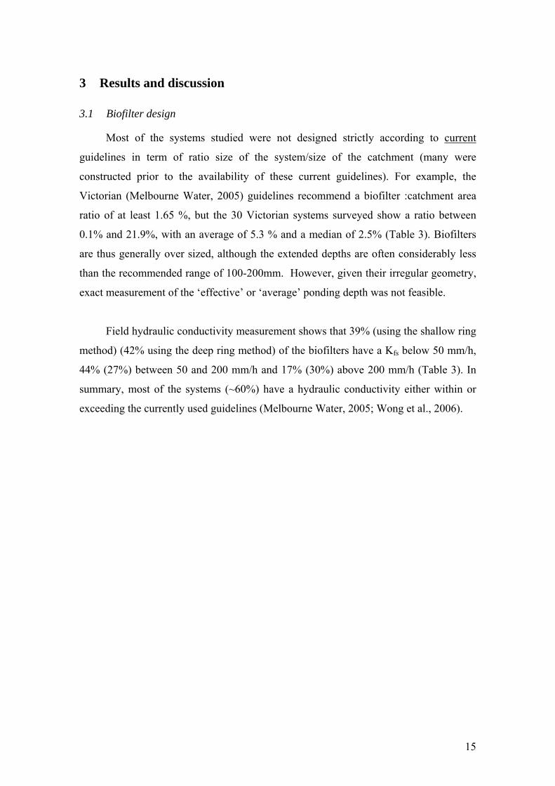
3.1 Biofilter design

Most of the systems studied were not designed strictly according to current

guidelines in term of ratio size of the system/size of the catchment (many were

constructed prior to the availability of these current guidelines). For example, the

Victorian (Melbourne Water, 2005) guidelines recommend a biofilter :catchment area

ratio of at least 1.65 %, but the 30 Victorian systems surveyed show a ratio between

0.1% and 21.9%, with an average of 5.3 % and a median of 2.5% (Table 3). Biofilters

are thus generally over sized, although the extended depths are often considerably less

than the recommended range of 100-200mm. However, given their irregular geometry,

exact measurement of the ‘effective’ or ‘average’ ponding depth was not feasible.

Field hydraulic conductivity measurement shows that 39% (using the shallow ring

method) (42% using the deep ring method) of the biofilters have a Kfs below 50 mm/h,

44% (27%) between 50 and 200 mm/h and 17% (30%) above 200 mm/h (Table 3). In

summary, most of the systems (~60%) have a hydraulic conductivity either within or

exceeding the currently used guidelines (Melbourne Water, 2005; Wong et al., 2006).

16

Table 3: Data for each site: hydraulic conductivity value (different method), catchment characteristics and

volume of water received

Hydraulic conductivity (mm/h) Sites characteristics Volume of water

Sites Kfs shallow ur(K) % Kfs deep ur(K) % Klab deep

(ini) Klab surf Age (year) Catchment

area (m²) Biofilter area (m²) Ratio (%) V. water/year

(m3) Total V. water

(m3) Total V./ m²

(m)

Streisand Dr, Brisbane 61 29 32 99 399 238 0.5 1105 20 1.8 1060.8 530.4 26.5

Saturn Cr, Brisbane 34 20 38 10 17 9 0.5 675 20 3.0 648.0 324.0 16.2

Donnelly Pl, Brisbane 19 22 63 12 12 0.2 1130 32.2 2.8 1084.8 217.0 6.7

Hoyland Dr, Brisbane 204 16 667 6 65 146 5 17400 860 4.9 16704.0 83520.0 97.1

58 30 68 14 53 0.5 1500 15 1.0 780.0 390.0 26.0

102 22 88 13 117 0.5 1500 15 1.0 780.0 390.0 26.0 Monash Car park, Clayton

45 20 55 15 48 0.5 1500 15 1.0 780.0 390.0 26.0

71 31 406 12 582 31 3 366 14.5 4.0 190.3 571.0 39.4

594 34 444 10 264 3 60 11 18.3 31.2 93.6 8.5

129 34 265 9 462 98 3 560 4.5 0.8 291.2 873.6 194.1

316 34 282 12 747 116 3 622 18 2.9 323.4 970.3 53.9

98 32 100 17 113 28 3 400 10 2.5 208.0 624.0 62.4

119 25 203 9 297 113 3 324 11 3.4 168.5 505.4 45.9

53 26 202 17 151 4 3 84 6 7.1 43.7 131.0 21.8

Cremorne St, Richmond

85 25 140 11 270 102 3 85 10 11.8 44.2 132.6 13.3

49 27 5 50 10 2 68 12 17.6 35.4 70.7 5.9

35 34 6 39 20 2 112 24.5 21.9 58.2 116.5 4.8

5 29 9 79 21 2 213 17 8.0 110.8 221.5 13.0 Aleyne St, Chelsea

19 30 8 50 12 2 163 22 13.5 84.8 169.5 7.7

139 25 321 7 246 1 410 7 1.7 213.2 213.2 30.5 Point Park, Docklands

135 20 77 47 306 1 370 7 1.9 192.4 192.4 27.5

36 14 7 76 5 3 3200 4 0.1 1664.0 4992.0 1248.0 Hamilton St, W. Brunswick

137 34 11 63 11 3 91 1 1.1 47.3 142.0 142.0

13 36 11 47 9 3 120 5 4.2 62.4 187.2 37.4

26 34 10 51 11 3 200 4 2.0 104.0 312.0 78.0 Avoca Cr, Pascoe Vale

44 34 6 59 15 3 310 4 1.3 161.2 483.6 120.9

24 34 23 30 4 3 314 12 3.8 163.3 489.8 40.8

19 21 56 13 16 3 157 14 8.9 81.6 244.9 17.5 Parker St, Pascoe Vale

39 34 1 138 7 3 528 7 1.3 274.6 823.7 117.7

Ceres, West Brunswick 97 19 60 13 2 1257 21.75 1.7 653.6 1307.3 60.1

Bourke St tree pit, Melbourne 84 23 23 21 1 100 1.44 1.4 52.0 52.0 36.1

Hallam Bypass, Floret Pl 154 24 199 63 3 120

Hallam Bypass, Wanke Rd 115 22 490 387 3 12

Hallam Bypass, Wanke Rd basin 203 27 286 207 3 168

Wolseley Pd, Vic Park (NSW) 159 18 425 5 376 560 7 1504 330 21.9 1413.3 9893.0 30.0

Leyland Gr, Vic Park (NSW) 237 17 398 4 151 224 7 1804 180 10.0 1695.8 11870.3 65.9

2nd Pond Creek (NSW) 5 21 2000 0

17

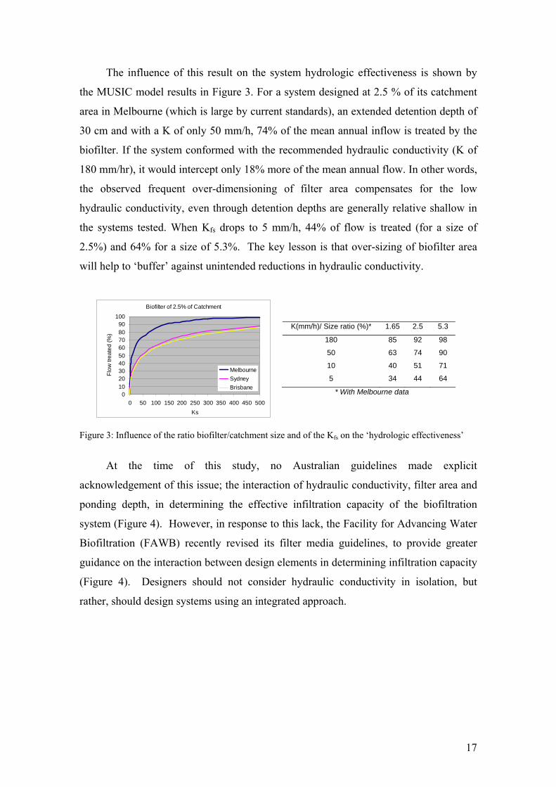
The influence of this result on the system hydrologic effectiveness is shown by

the MUSIC model results in Figure 3. For a system designed at 2.5 % of its catchment

area in Melbourne (which is large by current standards), an extended detention depth of

30 cm and with a K of only 50 mm/h, 74% of the mean annual inflow is treated by the

biofilter. If the system conformed with the recommended hydraulic conductivity (K of

180 mm/hr), it would intercept only 18% more of the mean annual flow. In other words,

the observed frequent over-dimensioning of filter area compensates for the low

hydraulic conductivity, even through detention depths are generally relative shallow in

the systems tested. When Kfs drops to 5 mm/h, 44% of flow is treated (for a size of

2.5%) and 64% for a size of 5.3%. The key lesson is that over-sizing of biofilter area

will help to ‘buffer’ against unintended reductions in hydraulic conductivity.

Biofilter of 2.5% of Catchment

0102030405060708090

100

0 50 100 150 200 250 300 350 400 450 500Ks

Flow

trea

ted

(%)

MelbourneSydneyBrisbane

K(mm/h)/ Size ratio (%)* 1.65 2.5 5.3

180 85 92 98

50 63 74 90

10 40 51 71

5 34 44 64

* With Melbourne data

Figure 3: Influence of the ratio biofilter/catchment size and of the Kfs on the ‘hydrologic effectiveness’

At the time of this study, no Australian guidelines made explicit

acknowledgement of this issue; the interaction of hydraulic conductivity, filter area and

ponding depth, in determining the effective infiltration capacity of the biofiltration

system (Figure 4). However, in response to this lack, the Facility for Advancing Water

Biofiltration (FAWB) recently revised its filter media guidelines, to provide greater

guidance on the interaction between design elements in determining infiltration capacity

(Figure 4). Designers should not consider hydraulic conductivity in isolation, but

rather, should design systems using an integrated approach.

18

Figure 4. Design elements that influence infiltration capacity (source: www.monash.edu.au/fawb).

3.2 Comparing field methods

Statistically both methods give similar results (p=0.38 for n=32). Correlation

between two methods is moderately strong with R² = 0.44 (Figure 5). This result can be

explained by the similarity between the two methods, which are both a pressure test

applied on the same surface of soil. The differences could be explained by the

uncertainty on each reading (around 30% as shown in Table 3) and by the spatial

variability in the systems. Contribution to uncertainty of the latter can be evaluated at

50% as shown in Table 4, based on repeated application of the hydraulic conductivity

measurements in one system. Since tests have not been conducted in the same spot it

could explain the moderate correlation.

y = 1.00x + 40.53R2 = 0.44

0

200

400

600

0 200 400 600Kfs shallow (mm/h)

Kfs

deep

(mm

/h)

Kfs shallow Kfs deep Mean (mm/h) 100 140 σ (mm/h) 115 172

Cv (%) 115% 123% n 32 p 0.38*

* logged transformed data to respect the normality for Kfs deep

Figure 5 : Correlation between field methods

filter media hydraulic

conductivity conductivity

extended detention

depth

filter surface

area

infiltration capacity

19

Table 4 : K value and Cv for each site

Shallow method Deep method

Sites n K (mm/h) Cv (%) n K (mm/h) Cv (%)

Cremorne St, pod7, Richmond 3 119 29 3 203 32

Cremorne St, pod9, Richmond 3 85 55 3 140 54

Parker St, pod 2 Pascoe Vale 3 19 46 3 56 48

Ceres, Brunswick East 4 97 63 4 60 73

Hamilton St pod1, Brunswick West 3 36 52

Monash car park, strip 1 4 58 34

Monash car park, strip 2 3 102 58

Monash car park, strip 3 3 45 33

Point park car park, Docklands, pod2 3 135 28

Alleyene st, Chelsea, pod4 3 19 140

Tree pit, Docklands, pod7 3 84 78

Hallam Bypass, Wanke Rd 3 115 55

Hoyland St 6 204 59 3 667 32

Donnelly Pl 3 19 58

Saturn dr 3 34 16 3 38 67

Wolseley Pd, Vic Park 5 159 63 5 425 80

Leyland Gr, Vic Park 5 237 55 5 398 21

2nd Pond Creek 9 5 67

Average 78 53 221 53

3.3 Comparing field and laboratory methods

The shallow field method gives results that are not statistically different from the

measurement made in the laboratory on samples taken from the surface (p=0.71, n=16).

The consequence of this is that there is very little bias introduced by the choice of

method. It is therefore possible to compare measurement from the field (shallow

method) and from the lab without effect of the method. These results are similar to that

of Reynolds et al.(2000), which showed for a sand and a loam, that the hydraulic

conductivity measured in the field (shallow method) does not vary significantly from

laboratory measurements (p>0.05, n=12 for the sand, n=10 for the loam).

20

The correlation between methods is low (R²=0.08). It can be explained by the

spatial variability of the hydraulic conductivity and by the variations in compaction

between the samples. In the laboratory, measurements are conducted on disturbed

samples (inevitably during sampling) that have been re-compacted to a standard value

which may be different than that which existed in the field. It may also be speculated

that another reason for lower K found in the laboratory measurements is due to the

samples being taken right at the surface; they therefore represent deposition formed over

time (i.e. they are deposited stormwater sediment). In this way Klab, surf represents the

hydraulic conductivity of the clogging layer on its own.

If we compare the results from the deep field tests and the laboratory tests, results

are statistically different (p<0.01 n=11). Importantly, these methods cannot be directly

compared, because they have a relatively low correlation (R²=0.11).

y = 0.57x + 70.47R2 = 0.08

0

200

400

600

0 200 400 600Kfs shallow (mm/h)

Kla

b su

rf (m

m/h

)

Kfs shallow Klab surf Mean (mm/h) 133 147 σ (mm/h) 76 151

Cv (%) 57% 103% n 16 p 0.71

Figure 6 : Correlation between field method and laboratory method on surface samples

3.4 Clogging of systems over time

Comparing results of the field experiments (which both provide an estimate of the

current system conductivity) and laboratory measurements on deep samples (which

provide an estimate of the initial conductivity) provides an indication of the evolution of

hydraulic conductivity since construction. Sediment deposition is considered to be the

principal cause of clogging (Bouwer, 2002) and can occur at the surface of the system

with the creation of a clogged layer (surface clogging) or deeply, by filling of the pore

space (interstitial clogging), as explained by Langergraber et al. 2003 and Winter et al.

21

(2003). Since both field measurements of the hydraulic conductivity give similar results

(average value: Kfs deep = 140 mm/h, Cv=123% and Kfs shallow =100 mm/h, Cv=115%), it

is evident that hydraulic conductivity of the system is controlled primarily by the top

layer and that there is no deep ‘clogging’ of the soil media.

However, vegetation development and especially root growth, will lead to the

creation of macropores. For example, Archer et al. (2000) showed that root growth

increases hydraulic conductivity, as root dieback creates macropores which facilitate

water movement in the soil. It is not yet clear whether this phenomenon will have a

major impact on biofilter hydraulic conductivity; if clogging is primarily occurring on

the surface, macropores below the clogged layer at the top may have little or no

consequence.

Results of the Ascendant Hierarchical Classification show four groups with

distinctly different behaviour. Group 1 has only one biofilter, which is undersized (0.1

% of the catchment); group 2 has three systems with very high Kfs (Kfs shallow average =

200 mm/h) and very high initial K (Klab deep ini average = 197 mm/h). Groups 3 and 4

represent 88% of the systems tested. Biofilters from group 3 have a high initial K (Klab

deep ini average = 241 mm/h, n=17), whilst group 4 systems have a low initial K (Klab deep

ini average= 12 mm/h, n=11).

Systems with a high initial hydraulic conductivity (which can be explained by

media with relatively coarse particles and a subsequently large pore space) will decrease

substantially over time, and proportionally by a greater amount than will systems with a

low initial hydraulic conductivity. This is demonstrated by the fact that the field

shallow test results show a hydraulic conductivity on average 114 mm/h (n=17) lower

than the laboratory deep tests as shown on Figure 7. This result is also confirmed by the

difference between the laboratory tests taken on the deep and surface samples, with an

average difference of 255 mm/h (n=9).

22

Figure 7 : Klab deep ini vs. Kfs shallow – white triangle, system with low initial hydraulic conductivity, black square, systems with high initial hydraulic conductivity

This decrease can be explained by sediment deposition at the surface. However,

final hydraulic conductivities are still relatively high (Kfs shallow = 127 mm/h, n=17), and

likely to be adequate to ensure good pollutant removal performance. This observation

may be either because the systems are only partially clogged, or because creation of

macropores is having some effect in creating flow through the media, possibly even at

the surface (for example, at the base of plant stems, where growing, senescence and

even stem movement due to wind, may cause ‘breaking up’ of any clogging layer)

(Figure 8).

Figure 8 : Schematic representation of the evolution of the behaviour of biofilters with high initial K

Klab deep ini = 241 Kfs shallow = 127 mm/h

23

Systems with low initial hydraulic conductivity (explained by a high concentration in

fine particles and thus a low pore volume) show effectively no decrease over time (ΔK

average = +25 mm/h, n=11; Figure 7). In part, this is because the relative difference in

particle size of the filter media, and of the influent sediment, will be less, meaning that

any buildup of sediment at the surface will have proportionally less impact. The slight

increase could again be contributed to by macropore creation by roots (Figure 9),

although further studies are required to test this hypothesis.

Figure 9 : Schematic representation of the evolution of the behaviour of biofilters with low initial K

3.5 Influence of system characteristics and hydraulic performance

Of all the factors tested – age of the biofilter, its initial hydraulic conductivity, the

ratio between its size and the size of the catchment drained, the volume of water

received per year and the volume of water received per m² of system since its

construction – only the initial conductivity provided a statistically significant

explanation of variability in current conductivity of the systems (Table 5).

Kfs shallow = 37 mm/h Klab deep in = 12 mm/h

24

Table 5: Regression between Kfs shallow and various parameters Field method Kfs shallow

R² 0.52 Parameters P value

(Constant) 0.00

Klab deep (ini) 0.00

Age 0.24

Ratio 0.34

Volume of water/year excluded

Total volume/m² 0.49

Achleitner et al. (2006) reported a similar lack of correlation between hydraulic

conductivity and site characteristics, and made the hypothesis that current K was mainly

governed by the initial value. This result is in some ways unfortunate, because it

provides little guidance to those charged with the maintenance of such systems, in being

able to predict their lifespan and maintenance requirements. However, it does show the

importance of correctly specifying the filter media during the biofilter design, and of

having appropriate quality control to ensure that the supplied and installed media meets

these specifications.

One approach is to use a “contingency factor” in the specification of hydraulic

conductivity for biofiltration systems. For example, where the design intent is to use a

soil media with a hydraulic conductivity of 180 mm/hr, sizing of the system should be

undertaken assuming a hydraulic conductivity of 50% of the design value (ie. 90

mm/hr). In this way, if the media does not meet specifications, or shows a decline in

hydraulic conductivity over time, the overall system performance will remain

satisfactory.

25

4 Conclusions

Whilst biofilters have been demonstrated to provide effective stormwater quality

treatment, their long-term hydraulic behaviour has to date not been studied, particularly

in reference to real systems. This study provides a first attempt to evaluate performance

of a range of constructed systems, with design and catchment characteristics.

From a measurement point of view, the different field methods used gave similar

results, demonstrating that for these soil-based biofilters, hydraulic conductivity is

governed by their surface layer. Field and laboratory experiments gave identical

results.

Regarding system design and construction, three key messages are deduced.

Firstly, whilst many systems measured have a low hydraulic conductivity (lower

than currently recommended values), a tendency by designers to over-dimension the

systems (relative to guidelines) acts to compensate for the low conductivity. Critically,

however, current guidelines do not address this relationship, and seem to pay no

attention to the risks of diminished effectiveness when systems are either constructed

with lower-than-desired conductivity, or when clogging causes conductivity to decline

over time. In particular, this may occur as a result of poor construction management

practices in the catchment, resulting in excessive sediment loading. Strict controls

should be in place during the construction phase of development.

Secondly, proportional hydraulic conductivity reduction occurs mainly for

systems with high initial value, but the resulting value ends up generally respecting the

guidelines. Other systems, which have been constructed with low-conductivity soils, do

not show evidence of further decline, possibly because the filter media particle size

distribution is more similar to that of the influent sediment, than is the case for systems

with high initial conductivity (and thus coarse media). Declines in conductivity over

time are likely to occur by sediment deposition, which occurs at the surface of the

systems. Whilst macropore creation by vegetation may limit the effect of clogging,

further detailed research is needed to verify the reliability of this strategy in maintaining

soil hydraulic conductivity within recommended guidelines.

26

Finally, it was not possible to predict a filter’s current hydraulic conductivity from

factors such as its size, the catchment size, or the inflow volume. The initial specified

hydraulic conductivity is the critical determinant of its long-term hydraulic behaviour.

Whilst this provides little help in predicting system lifespan or maintenance

requirements, it does reinforce the criticality of specifying the correct hydraulic

conductivity of systems at the time of construction. Perhaps most importantly,

guidelines do not pay due attention to the importance of translating design

specifications through the construction process. Contract hold-points should in place to

ensure testing of the media during construction.

5 Acknowledgments

The authors would particularly like to thank Peter Poelsma at the Facility for

Advancing Water Biofiltration for help in the field experiments. Support from

Melbourne Water is also gratefully acknowledged.

27

6 References

Achleitner S., Engelhard C., Stegner U. and Rauch W. Local infiltration devices at parking sites-Experimental assessment of temporal changes in hydraulic and contaminent removal capacity, WSUD 2006, Melbourne

Archer N. A., Quniton J. N. and Hess T. M. Below ground relationships of soil texture, roots and hydraulic

conductivity in two-phase mosaic vegetation in South-east Spain. Journal of Arid Environments, 2002, Vol. 52, p 535-553

AS 4419—2003, Australian Standard, Soils for landscaping and garden use, appendix H, Method of

determining the permeability of a soil. Bouwer Herman. Artificial recharge of groundwater: hydrogeology and engineering. Hydrogeology Journal,

2002, Vol. 10, p 121-142. Brown R. and Clarke J. The transition towards water sensitive urban design : a socio-technical analysis of

Melbourne, Australia, Novatech 2007 Sustainable techniques and strategies in urban water management, Lyon, France, June 2007, p 349- 356

Bureau of Meteorology, < www.bom.gov.au> Daniel D. E. In situ hydraulic conductivity tests for compacted clay. Journal of Geotechnical Engineering,

1989, Vol. 115 (9) Dietz M.E. and Clausen J.C. Stormwater runoff and export changes with development in a traditional and

low impact subdivision. Journal of Environmental Management (2007) (sumitted) Gardner W.R. Some steady-state solutions of the unsaturated moisture flow equation with application to

evaporation from a water table. Soil Sci., 1958, Vol. 85, p 228–232. Hatt, B. E., N. Siriwardene, A. Deletic and T. D. Fletcher. Filter media for stormwater treatment and

recycling: the influence of hydraulic properties of flow on pollutant removal. Water Science and Technology, 2006, Vol. 54(6-7), p 263-271.

Langergraber G., Haberl R., Laber J. and Pressi A. Evaluation of substrate clogging processes in vertical

flow constructed wetlands. Water Science an Technology, 2003, Vol. 48(5), p 25 -34 Lindsey G, Roberts L. and Page W. Inspection and maintenance of infiltration facilities, J. Soil and Water

Cons., 1992, Vol. 47 (6), p 481-486 Melbourne Water (2005). Water Sensitive Urban Design (WSUD) Engineering procedures: stormwater.

Chapter 6 Bioretention basins CSIRO publishing, 2005, Melbourne National Institute of Standards and Technology (NIST), United States Department of Commerce

Technology Administration, Technical Note 1297, Guidelines for Evaluating and Expressing the Uncertainty of NIST Measurement Results (1994)

Reynolds W. D. and Elrick D. E. Ponded infiltration from a single ring: Analysis of steady flow. Soil Sci.

Soc. Am., 1990, Vol. 54, p. 1233-1241 Reynolds W. D., Bowman B. T., Brunke R. R., Drury C. F. and Tan C. S. Comparison of tension

infiltrometer, Pressure infiltrometer, and soil core estimates of saturated hydraulic conductivity. Soil Sci. Soc. Am., 2000, Vol. 64, p 478-484

Schueler, T.R., Kumble, P.A. and Heraty, M.A. A Current Assessment of Urban Best Management

Practices, Techniques for Reducing Non-point Source Pollution in the Coastal Zone, Metropolitan Washington Council of Governments, 1992, Washington, D.C.

Victoria stormwater committee. Urban Stormwater Best Practice Environmental Management Guidelines.

CSIRO publishing, 1999 Winter K.-J. and Goetz D. The impact of sewage composition on the soil clogging phenomena of vertical

flow constructed wetlands. Water Science and Technology, 2003, Vol. 48(5), p 9-14

28

Wong, T. H. F. (Ed.). (2006). Australian runoff quality. Sydney, Australia: Institution of Engineers, Australia. Wong T. H. F., Breen P. F., Somes N. G. L. and Lloyd S. D. Managing Urban Stormwater Using

Constructed Wetlands. Melbourne, Australia: CRC for Catchment Hydrology and CRC for Freshwater Ecology Industry Report 98/7, 1999

Youngs E. G., Elrick D. E. and Reynolds W. D. Comparison of steady flows from infiltration rings in “Green

and Ampt” and “Gardner” soils. Water Resources Research, 1993, Vol. 29 (6), p 1647-1650 Zinger Y., Fletcher T. D., Deletic A., Blecken G. T. and Viklander M. Optimisation of the nitrogen retention

capacity of stormwater biofiltrations systems, Novatech 2007 Sustainable techniques and strategies in urban water management, Lyon, France, June 2007, p 893- 900