HYDRAULIC FRACTURE PROPAGATION MODELING

AND DATA-BASED FRACTURE IDENTIFICATION

by

Jing Zhou

A dissertation submitted to the faculty of The University of Utah

in partial fulfillment of the requirements for the degree of

Doctor of Philosophy

Department of Chemical Engineering

The University of Utah

May 2016

Copyright © Jing Zhou 2016

All Rights Reserved

The U n i v e r s i t y o f Ut ah G r a d u a t e S c h o o l

STATEMENT OF DISSERTATION APPROVAL

The dissertation of Jing Zhou

has been approved by the following supervisory committee members:

Milind D. Deo Chair 10/22/2015Date Approved

Mikhail Skliar Member 10/22/2015Date Approved

John D. McLennan Member 10/22/2015Date Approved

Hai Huang Member 10/22/2015Date Approved

Michael S. Zhdanov Member 10/22/2015Date Approved

and by Milind D. Deo Chair/Dean of

the Department/College/School o f ______________Chemical Engineering

and by David B. Kieda, Dean of The Graduate School.

ABSTRACT

Successful shale gas and tight oil production is enabled by the engineering innovation

of horizontal drilling and hydraulic fracturing. Hydraulically induced fractures will most

likely deviate from the bi-wing planar pattern and generate complex fracture networks

due to mechanical interactions and reservoir heterogeneity, both of which render the

conventional fracture simulators insufficient to characterize the fractured reservoir.

Moreover, in reservoirs with ultra-low permeability, the natural fractures are widely

distributed, which will result in hydraulic fractures branching and merging at the

interface and consequently lead to the creation of more complex fracture networks. Thus,

developing a reliable hydraulic fracturing simulator, including both mechanical

interaction and fluid flow, is critical in maximizing hydrocarbon recovery and optimizing

fracture/well design and completion strategy in multistage horizontal wells.

A novel fully coupled reservoir flow and geomechanics model based on the dual­

lattice system is developed to simulate multiple nonplanar fractures’ propagation in both

homogeneous and heterogeneous reservoirs with or without pre-existing natural fractures.

Initiation, growth, and coalescence of the microcracks will lead to the generation of

macroscopic fractures, which is explicitly mimicked by failure and removal of bonds

between particles from the discrete element network. This physics-based modeling

approach leads to realistic fracture patterns without using the empirical rock failure and

fracture propagation criteria required in conventional continuum methods. Based on this

model, a sensitivity study is performed to investigate the effects of perforation spacing,

in-situ stress anisotropy, rock properties (Young’s modulus, Poisson’s ratio, and

compressive strength), fluid properties, and natural fracture properties on hydraulic

fracture propagation.

In addition, since reservoirs are buried thousands of feet below the surface, the

parameters used in the reservoir flow simulator have large uncertainty. Those biased and

uncertain parameters will result in misleading oil and gas recovery predictions. The

Ensemble Kalman Filter is used to estimate and update both the state variables (pressure

and saturations) and uncertain reservoir parameters (permeability). In order to directly

incorporate spatial information such as fracture location and formation heterogeneity into

the algorithm, a new covariance matrix method is proposed. This new method has been

applied to a simplified single-phase reservoir and a complex black oil reservoir with

complex structures to prove its capability in calibrating the reservoir parameters.

iv

To my parents, Jianhua Zhou and Li Li

To my husband, Jixiang Huang

TA BLE OF C O N T EN TS

ABSTRACT.................................................................................................................................iii

ACKNOWLEDGEMENTS...................................................................................................... ix

Chapters

1. INTRODUCTION................................................................................................................. 1

1.1 Challenges in Estimating the Hydraulic Fracturing Process............................... 31.2 Numerical Simulation of Hydraulic Fracture Propagation..................................6

1.2.1 Numerical Methods Description................................................................. 61.2.2 Previous Numerical Model in Predicting Hydraulic Fracture Propagation............................................................................................................... 8

1.3 Research Objectives................................................................................................17

2. HYDRAULIC FRACTURE SIMULATOR.....................................................................23

2.1 Introduction.............................................................................................................. 242.2 Dual Lattices............................................................................................................25

2.2.1 Rock DEM Lattice Genesis Procedure..................................................... 252.2.2 Conjugate Flow Lattice-Genesis Procedure.............................................28

2.3 The Assumptions Made in our DEM Model....................................................... 292.4 The Algorithm of Fracture Propagation Based on Dual-Lattice DEM ............30

2.4.1 Geomechanics Calculation.........................................................................322.4.2 Pressure Calculation....................................................................................412.4.3 Coupling Pressure Calculation with Geomechanics.............................. 462.4.4 Failure Criterion.......................................................................................... 462.4.5 Complete Numerical Procedure................................................................ 48

2.5 The Advantages of Dual-Lattice Discrete Element Method............................. 49

3. MULTIPLE HYDRAULIC FRACTURES’ PROPAGATION IN HOMOGENEOUS RESERVOIR ........................................................................................................................61

3.1 Hydraulic Fracture Propagation from Single W ellbore.....................................623.1.1 Two Hydraulic Fractures Propagate Simultaneously............................. 633.1.2 Two Hydraulic Fractures Propagate Sequentially...................................65

3.1.3 Multiple Hydraulic Fractures Propagate Simultaneously.......................673.1.4 Sensitivity Analysis.....................................................................................70

3.2 Hydraulic Fracture Propagation from Multiple W ellbores............................... 773.3 Summary.................................................................................................................. 78

4. HYDRAULIC FRACTURE PROPAGATION IN HETEROGENEOUS RESERVOIR........................................................................................................................91

4.1 Simplified Heterogeneous Model with Three Layers........................................ 924.1.1 Permeability Heterogeneity........................................................................924.1.2 Mechanical Heterogeneity.......................................................................... 93

4.2 Field Heterogeneous Reservoir............................................................................. 944.2.1 Coarse Model - Reservoir with Five Layers........................................... 954.2.2 High Resolution Model - Reservoir with 24 Layers.............................. 96

4.3 Summary.................................................................................................................. 98

5. INTERACTION BETWEEN HYDRAULIC FRACTURES AND NATURAL FRACTURES.....................................................................................................................107

5.1 Introduction............................................................................................................1075.2 Representation of Natural Fractures.................................................................. 1125.3 Simple Case of HF and NF Interaction.............................................................. 1135.4 Sensitivity Analysis..............................................................................................115

5.4.1 Effect of Natural Fracture Orientation................................................... 1165.4.2 Effect of Natural Fracture Cohesion...................................................... 1175.4.3 Effect of Natural Fracture Permeability.................................................1185.4.4 Effect of Injection R ate ............................................................................ 1195.4.5 Effect of Injection Viscosity.....................................................................1205.4.6 Effect of Stress Anisotropy......................................................................121

5.5 Summary................................................................................................................ 123

6. COMBINATION OF REALISTIC FRACTURE GEOMETRY WITH FLOW SIMULATOR .....................................................................................................................132

6.1 Mapping of the Hydraulic Fracture.....................................................................1326.2 Flow R esults..........................................................................................................1346.3 Summary................................................................................................................ 135

7. DATA ASSIMILATION.................................................................................................. 143

7.1 Introduction............................................................................................................1447.2 The Algorithm of Ensemble Kalman Filter...................................................... 1497.3 Uncertainty Covariance Matrix M ethod............................................................1517.4 Illustrative Exam ples........................................................................................... 155

7.4.1 Single-Phase Reservoir with Two Fractures......................................... 155

vii

7.4.2 Three-Phase Black Oil Reservoir - PUNQ-S3 M odel.........................1657.5 Summary................................................................................................................ 167

8. CONCLUSIONS AND FUTURE W ORK.....................................................................179

8.1 Summary of Research W ork............................................................................... 1798.2 Recommendations of Future W ork.....................................................................181

REFERENCES.........................................................................................................................184

viii

A C K N O W L E D G E M E N T S

First and foremost, I would like to express my deepest and sincere gratitude to my

advisor, Professor Milind D. Deo, who provided guidance, knowledge and

encouragement throughout my Ph.D. study at University of Utah. He is a knowledgeable,

kind and patient mentor. I also want to extend my appreciation to my co-advisor, Dr.

Mikhail Skliar, for his guidance and support.

I am also extremely grateful to my committee member, Dr. Hai Huang from Idaho

National Laboratory for helping me dig into geomechanics. He is always patient in

discussing research problems with me and consistently comes up with valuable and

critical ideas. I would like to thank my other committee members: Dr. John McLennan

and Dr. Michael Zhdanov for their insightful comments and suggestions.

The help and support from the rest faculty and staff of Chemical Engineering

Department are also greatly appreciated. I would like to thank ConocoPhillips for

providing fellowship during my study. I also would like to thank the faculty and staff in

Energy & Geoscience Institute.

I would like to thank my officemates at the Petroleum Research Center for their help

during my research time. I also want to thank all my friends at Salt Lake City, who I

regard as a family, for making my life wonderful and unforgettable. I would like to thank

all friends I met at Idaho Falls during my two summer internships,

who make that time precious and memorable.

Finally, I would like express my gratitude to my parents, Jianhua Zhou and Li Li, for

their endless love and support as well as consistent encouragement in the tough time. I

owe special thanks to my husband, Jixiang Huang, for helping and encouraging me since

high school. I cannot imagine my life without him.

x

C H A PT E R 1

INTRODUCTION

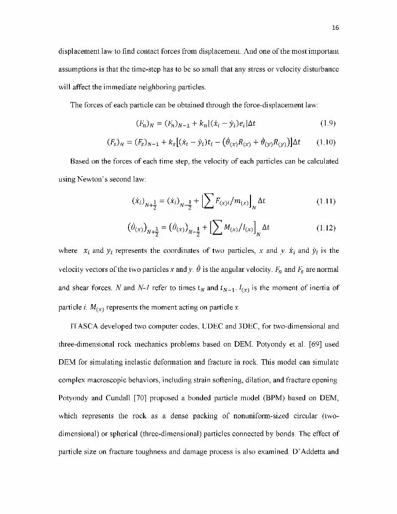
Based on U.S. Energy Information Administration (EIA) estimations, net U.S. imports

of energy declined from 30% of total energy consumption in 2005 to 13% in 2013. As

shown in Figure 1.1, with high oil price, and abundant oil and gas resources, the United

States will become a net energy exporter in 2019. However, if oil prices are low, the United

States will remain a net energy importer through 2040 [1]. The tendency of reducing

dependence on energy importation is the result of significant growth in domestic crude oil

and dry natural gas production from the exploration of tight oil and shale gas reservoirs in

recent years (Figure 1.2).

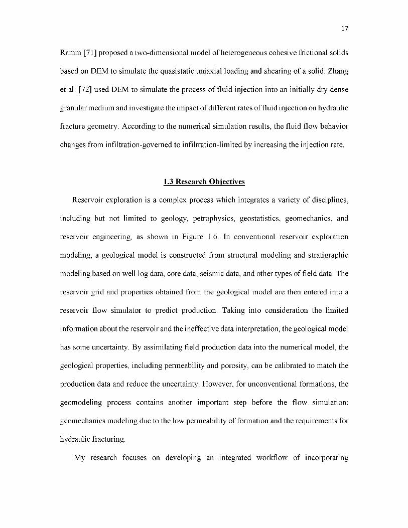
The production from tight oil formations leads the growth in US crude oil production.

Due to the decreasing domestic consumption of liquid fuels and increasing crude oil

production, the net import percentage of crude oil will decrease from 33% in 2013 to 17%

in 2040. Total dry natural gas production has increased by 35% from 2005 to 2013.

According to the EIA 2015 Annual Energy Report, the total shale gas production (including

natural gas from tight oil formations) will increase from 24.4 Tcf in 2013 to 35.5 Tcf in

2040, which is almost a 45% increase compared with current production. Production

growth is largely attributed to the development of shale gas resources in the Lower 48

states, such as the Haynesville and Marcellus formations.

Unconventional formations such as shale gas or tight oil have two special features that

differentiate them from conventional reservoirs [2]: 1. ultra-low permeability (at the order

of nanodarcy) 2. pre-existing natural fractures. Because of the low permeability, it is very

difficult or almost impossible for the hydrocarbon to flow through the porous media and

reach to wellbore relying only on its own permeability. And the presence of natural

fractures will result in a more complex fracture network due to the hydraulic and natural

fractures’ interactions.

Two key technologies enable the successful recovering of hydrocarbon from

unconventional reservoirs: horizontal drilling and multistage hydraulic fracturing. The

generated hydraulic fracture can provide an additional high-conductivity path from

formation to wellbore. Therefore, the contacting surfaces generated by hydraulic fracturing

determine the estimated ultimate recovery (EUR). In order to improve production, ten to

twenty or more fracture stages are employed in the horizontal wellbore, and each stage

includes three to six perforation clusters to initiate fractures.

The hydraulic fracturing process can be described as follows [3]: At the first step,

multiple perforations are created along the horizontal wellbore and result in several weak

points in the formation. Then fracking fluids such as slickwater or viscous gel are pumped

into the wellbore, which lead to a rapid pressure accumulation. A certain time after

injecting, high pressure will break the rock and fractures will initiate and propagate at the

predefined perforations.

Generally, clean fluid, known as pad, is pumped firstly for creating sufficient fracture

width. Then proppant will be injected to maintain the opening of induced hydraulic

fractures. The whole process takes a relatively short time, varying from minutes to hours,

2

depending on the size of reservoir and the expected fracture volume. When the pumping

stops, the residual fluid will leak from the fracture into the formation, which makes the

fracture surfaces close onto the proppant particles under the compressive stress. Finally, a

conductive flow path filled with proppant is formed through the hydraulic fracturing

process.

1.1 Challenges in Estimating the Hydraulic Fracturing Process

Hydraulic fracturing is a well-stimulation technique which creates fractures in rock

formations through the injection of hydraulically pressurized fluid. It first appeared in the

oil and gas industry in the 1930s when Dow Chemical Company got more effective acid

stimulation by deforming and fracturing rock formations[4]. The first nonacid hydraulic

fracturing for well stimulation happened in 1947. And since the 1950s, about 70% of gas

wells and 50% of oil wells have been hydraulically fractured[5]. Currently, fracking fluids

are utilized extensively in fields, including low permeability gas formations, weakly

consolidated offshore sediments, “soft” coal beds, and naturally fractured reservoirs, to

stimulate oil and gas wells [3]. Wide and successful applications of horizontal wells and

hydraulic fracturing are the key reasons leading the exponentially growth of tight oil and

shale gas production.

Due to the crucial role of additional contacting surface generated by fractures on oil

and gas recovery, the industry would like to optimize the stimulation strategy to maximize

the created hydraulic fractures. While in the fracture designing process, the primary

objectives include:

(1) Generating sufficient fracture length and height in contact with reservoir

3

(2) Improving and maintaining the hydraulic fracture conductivity through proppant

injection

(3) Determining well locations, number of stages/perforations, and injected fluid

properties with consideration of in-situ stress and formation rock type

There are several challenges in precisely predicting and controlling the induced fracture

geometry because of the complexity of unconventional reservoirs [6].

1.1.1 Fractures’ Mechanical Interaction

The most important and particular feature of hydraulic fracturing is that the opening of

fractures will continuously change the local stress magnitude and orientation, which is

called a stress shadow effect. This effect will further affect the induced fracture pattern in

multiple-fracture propagation. There are various forms of interactions between hydraulic

fractures: in-stage fracture-fracture interaction, stage-stage interaction, and multiple

horizontal wellbores interaction. All of these interactions will alter the fracture pattern from

bi-wing planar geometry to the formation of complex fracture networks, as shown in Figure

1.3.

1.1.2 Reservoir Heterogeneity

Rock is a heterogeneous material containing many natural weaknesses, including pores,

grain boundaries, and pre-existing fractures [7]. Microseismic monitoring, production data,

log, and seismic data confirm that the reservoir formation has strong lateral heterogeneity,

which is a key impact factor of rock’s mechanical behaviors. During the hydraulic

fracturing process, these pre-existing weaknesses can induce microcracks or

4

microfractures, which can in turn change the flow capability of the rock. For example, the

Bakken formation is a layered heterogeneous reservoir, which has been separated into

upper, middle, lower and three forks. And even in one layer, the rock mineralogy varies

with depth and location. Thus, without considering the intrinsic heterogeneity, the

predicted morphology of hydraulic fracture may be biased and misleading in guiding the

horizontal well completion strategy.

1.1.3 Existence of Natural Fractures

In an unconventional reservoir with ultra-low permeability, such as Barnett, the natural

fractures are widely distributed. When the hydraulic fracture approaches the natural

fractures, it will have different scenarios of hydraulic-natural fractures interaction, such as

branching and merging and consequently lead to complex fracture network (Figure 1.4).

The reactivation of natural fractures will also provide an effective flow path to connect

formation to wellbore.

1.1.4 Insufficient Information From Microseismic Data

Generally, microseismic events are very small-scale earthquakes as a result of industry

processes, such as mining, hydraulic fracturing, enhane oil recovery, geothermal

operations, and underground gas storage. Many researchers and industry companies also

utilize microseismic data to estimate fracture geometry. Through mapping those

microseismic data, the general idea about stimulated reservoir volume will be obtained.

Moreover, the intensity and linear treads of microseismicity can indicate the degree of

fracturing and major fluid pathways during fracturing [8]. However, the resolution of this

5

data is too rough to describe the exact hydraulic fracture planes. Moreover, the

microseismic data cannot predict the detailed growing and interacting behaviors of

hydraulic fractures.

1.2 Numerical Simulation of Hydraulic Fracture Propagation

1.2.1 Numerical Methods Description

To adequately represent rock and simulate rock behavior in computational models, the

following features should be captured in the numerical model conceptualization: 1. rock

behavior and the physical mechanism under different stress loadings as described by

constitutive relationship; 2. the pre-existing stress, temperature and pressure conditions; 3.

the heterogeneous and anisotropic rock properties.

The most widely used numerical methods for rock mechanics problems are: 1.

continuum methods, including Finite Difference Method (FDM), Finite Element Method

(FEM), Boundary Element Method (BEM), and Extended Finite Element Method

(XFEM); 2. discontinuum methods, such as Discrete Element Method (DEM) and Discrete

Fracture Network Method (DFN) [9]; 3. hybrid continuum/discontinuum models such as

hybrid FEM/BEM model, hybrid FEM/DEM model [10].

The finite difference method is the oldest and most direct numerical method. The

fundamental principal of FDM is replacing partial derivative in governing PDEs with

difference at regular or irregular grids. This method is easy to implement. However, due to

its inflexibility in dealing with fractures, complex boundary conditions, and material

inhomogeneity, it is unsuitable for analyzing rock mechanics problems.

The finite element method was first introduced in structural analysis and used for plane

6

stress problems in 1960 [11]. The FEM required the discretization of the domain into many

smaller elements with standard shapes, including triangular, tetrahedral, and quadrilateral.

Trial equations are used to approximate the behavior of PDEs at the element level and

generate local algebraic equations to represent the behavior of different elements. Then the

local elemental equations are assembled into a global system of algebraic equations based

on topologic relations between nodes and elements. Therefore, the implementation of FEM

includes three steps: domain discretization, local approximation, and assemblage and

solution of the global matrix equation. The finite element is the most widely applied

numerical method because of its capability in handling material heterogeneity,

nonlinearity, and complex boundary conditions.

However, the FEM is not suitable for solving very large domain problems. The

efficiency of this algorithm decreases with the increasing nodes and degrees of freedom.

With the assumption of a general continuum, the block rotation, complete detachment and

large scale fracture opening cannot be obtained based on FEM formulations. Moreover, in

the finite element framework, crack initiation and growth are implemented by repeatedly

applying remeshing, a strategy which will further increase the computational cost [12].

The boundary element method only requires discretization at the boundary of the

solution domain. Unlike FDM and FEM, it approximates the solutions locally only at

boundary elements by trial functions. The boundary integral equation method was firstly

used by Jaswon [13] and Symm [14]. The application of this method to fracture mechanics

was proposed by Cruse in 1978 [15]. It has greater efficiency compared with FDM and

FEM because it reduces the problem dimensions by one. The BEM remains the optimal

numerical method for simulating fracture propagation in extremely large domains.

7

8

The discrete element method is a relatively new numerical method in modeling rock

mechanics. The essence of this method is to represent the rock as an assemblage of blocks.

The displacements caused by block motion and rotation are obtained through solving the

equations of motion. One significant advantage of this method is that the fracture opening

and complete detachment can be explicitly described in the DEM, which is impossible in

other numerical methods such as FDM, FEM or BEM.

1.2.2 Previous Numerical Model in Predicting Hydraulic Fracture Propagation

Hydraulic fracturing is a complex process, not only because of the severe heterogeneity

of reservoir structure and complex unknown in-situ stresses, but also because of the

complicated physics involved in the fracturing process. Hydraulic fracturing models have

evolved from two-dimensional models to three-dimensional models, from bi-wing planar

fracture geometry to dendrite-type complex fracture networks. Traditional hydraulic

fracturing simulators assumed single bi-wing planar fracture with a penny-shaped fracture

geometry extending from the wellbore to the formation. Fracture initiation and propagation

direction are obtained through the calculation of stress intensity factor and different criteria.

Usually, the theory of linear elasticity is used to model the rock deformation, the fluid flow

is simulated using lubrication theory, and the linear elastic fracture mechanics (LEFM)

theory is adopted to determine the fracture propagation [3], [16]. Two typical traditional

models used to predict the hydraulic fracture geometry are the Khristianovich-Geertsma-

DeKlerk (KGD) model [17], [18] and the Perkins-Kern-Nordgren (PKN) model [19], [20].

Both models assume the plane strain deformation (two-dimensional model) and calculate

fracture width based on the analytical solution [21]:

9

(1.1)

where w is the width/aperture along the crack, v is the rock’s Poisson’s ratio, E is the

Young’s modulus, p is the net pressure within the crack, and b is the fracture half-length.

The KGD model calculates the fracture propagation in the horizontal plane and

assumes no variation of fracture width in the vertical direction. The maximum fracture

width at the wellbore could be obtained using Equation (1.2). This KGD model is more

suitable for simulating fracture propagation in the early injection stage when the fracture

height is much larger than the fracture length.

On the contrary, the PKN model assumes plane strain for a fracture in the vertical plane,

which makes this model more accurate at late injection stage. Daneshy incorporated the

power-law fluid into the KGD model [22]. Spence and Sharp introduced rock toughness

into the model [23]. Both KGD and PKN models have limitations in their application

because they oversimplify the fracture propagation problems.

Based on these two-dimensional models, a series of pseudo-three-dimensional (P3D)

[24], [25] and true three-dimensional (3D) models [26], [27] are proposed to include

fracture height growth. All models allow the fracture to grow into different adjoining

layers. The propagating depth is determined by the layers’ properties and the stress

discrepancy between layers [28]. Simonson et al. [24] developed a P3D model to predict

fracture growth in a symmetric formation. Fung et al. [29] extended this method to an

asymmetric reservoir with a semianalytic technique. The P3D is an effective method to

capture the physical behavior of a planar three-dimensional hydraulic fracture. All the P3D

4(1 V ')pn,avg^ E

(12)

model can be classified into two categories: cell-based models and lumped models. In a

cell-based model, the fracture has been separated into many self-similar cells. In the

lumped approach, a fracture is assumed to consist of two half ellipses connected at the

fracture length direction [30]. The P3D models can efficiently estimate the fracture growth

in the vertical direction, without considering the fluid flow in that direction [5]. The true

3D model can model the fluid flow in both lateral direction and vertical direction, but the

computational cost is too large to promote extensive adoption, especially in field

applications. Moreover, all those methods cannot simulate the mechanical interactions

between fractures. Fractures propagate independently and will not be impacted by the stress

shadow induced by other fractures. Microseismic data from the Barnett case clearly show

that the predicted fracture length from a planar fracture model far exceeds the realistic

fracture length [31].

In order to account for the mechanical interactions and overcome the limitations of bi­

wing fracture models, a variety of hydraulic fracturing models have been proposed in

recent years. A reliable numerical simulator in estimating subsurface rock behavior should

at least be able to capture the physics evolved in the hydraulic fracturing process, which

includes

(1) Hydraulic fracture initiation and propagation,

(2) Fluid flow along the fracture and leakoff into formation,

(3) Mechanical interaction between induced fractures.

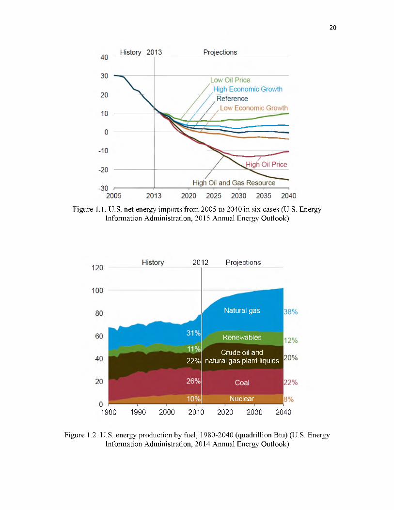
One widely used method is the displacement discontinuity method (DDM), which is an

indirect boundary element method developed by Crouch [32]. The concept of indirect

approach is to place the finite domain into a fictitious infinitely large domain to derive the

10

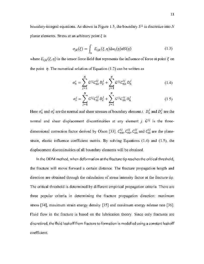
boundary-integral equations. As shown in Figure 1.5, the boundary S± is discretize into N

planar elements. Stress at an arbitrary point % is

°jk(0 = [ E i j k i ^ r i h U i W d S ^ ) (1.3)Js

where Etjk (^ ,y ) is the tensor force field that represents the influence of force at point ^ on

the point ^. The numerical solution of Equation (1.2) can be written as

N N^ GVcii Di + ^ GtJ'cHn Dl (1.4)i=i i=iN N

+ ^ G ‘l c g D i (1.5)j=1 j=1

Here and are the normal and shear stresses of boundary element i. and DJS are the

normal and shear displacement discontinuities at any element j. Gli is the three­

dimensional correction factor derived by Olson [33]. C'rln,C'rls,ClJn and ClJs are the plane-

strain, elastic influence coefficient matrix. By solving Equations (1.4) and (1.5), the

displacement discontinuities of all boundary elements will be obtained.

In the DDM method, when deformation at the fracture tip reaches the critical threshold,

the fracture will move forward a certain distance. The fracture propagation length and

direction are obtained through the calculation of stress intensity factor at the fracture tip.

The critical threshold is determined by different empirical propagation criteria. There are

three popular criteria in determining the fracture propagation direction: maximum

stress [34], maximum strain energy density [35] and maximum energy release rate [36].

Fluid flow in the fracture is based on the lubrication theory. Since only fractures are

discretized, the fluid leakoff from fracture to formation is modelled using a constant leakoff

coefficient.

11

a ls = Y G V C lsl D i

Dong and Pater [37] used DDM to model two-dimensional elastic fractures with

constant internal pressure. Olson [38] developed a pseudo-3D DDM simulator with the

assumption of zero-viscosity fluid injection. The fractures’ interaction only occurred in the

lateral plane. Cheng [39] described the stress distribution around multiple static fractures

to analyze fractures’ interaction based on DDM. Wu and Olson [40]-[42] proposed both a

two-dimensional and simplified three-dimensional nonplanar hydraulic fracturing

simulator based on DDM, and investigated the effects of perforation spacing and

simultaneous and sequential injection on an induced fracture pattern. Sesetty and Ghassemi

[43] also investigated the impact of injection strategies on fracture interactions based on

DDM. Hyunil Jo [44] examined the influence of fracture spacing on fracture geometry. In

his paper, the orientation of subsequent fractures gradually transits from repelling to

attracting the first fracture as a result of decreasing spacing between the fractures. Bunger

et al. [45] conducted a series of dimensional analyses and scale techniques to identify the

key parameters which lead to fracture curving using DDM-based simulator.

Compared with other methods, the DDM reduces the dimensions of the problem by

one through discretizing only the boundaries rather than whole domain. Therefore the

DDM exhibits higher computational efficiency and more accuracy, which makes it very

suitable for predicting fracture propagation with rapid stress change in a large field-scale

reservoir. However this model is not efficient in dealing with material heterogeneity and

nonlinear material behaviors.

Besides the displacement discontinuity method, a variety of analytical methods are also

used to simulate hydraulic fracturing propagation. Analytical solutions regain some

popularity for understanding different regimes of fracture propagation. Desroches et al.

12

[46] derived an analytical solution for zero-toughness and impermeable cases. Lenoach

[47] provided the analytical solution for zero-toughness, leak-off dominated cases. Those

solutions have shown that hydraulic fractures are controlled by toughness, viscosity or

leak-off dominated regimes [48]. Wong et al. [49] used an analytical model to describe

some salient features of multiple hydraulic fracture interaction in a viscous mass-transfer-

dominated regime. In order to reduce the computational burden, two fracture growth

patterns are defined: compacted fracture growth and diffuse fracture growth. In the

compact mode, the interactions and interferences between fractures are minimum. The

analytic model can provide quick insights into the controlling parameters and stimulation

optimization.

Roussel and Sharma [50], [51] used a three-dimensional finite difference method to

model stress perturbation by fixing the aperture of pre-existing fractures. The subsequent

fracture geometry is obtained based on the updated stress trajectories.

Yamamoto et al. [52] developed a hybrid three-dimensional simulator to predict the

multiple fractures’ propagation and interaction. The model iteratively coupled rock

deformation through DDM and fluid flow based on the finite element method. Castonguay

et al. [53] used a symmetric Galerkin boundary element method to calculate the

interactions between fractures and predict fracture geometry and propagation. The flow in

the fractures is simulated as a power-law fluid in arbitrary curved channels. Based on the

developed simulator, the impact of fractures numbers, fluid viscosity, and limited entry are

investigated.

Shin and Sharma [54] simulated multiple hydraulic fracture propagation using

ABAQUS Standard finite element analysis software. The reservoir is modeled as a porous

13

elastic medium, and pore pressure cohesive elements are inserted at each perforation cluster

to model fracture propagation. Based on this simulator, the effects of factors, such as

perforation cluster spacing, fluid viscosity, pumping rate, Young’s modulus, and fracture

height, on simultaneous propagation of multiple fractures within a single stage are

investigated. However, in this model, the fractures propagate only at predefined planes.

The simulators based on the finite-element method utilized various remeshing strategies to

explicitly simulate the crack propagation [12], [55], [56], which are inefficient and time

consuming for transferring the information between different meshes.

To avoid the remeshing issue and improve efficiency, the Extended Finite Element

Method (XFEM) is proposed [57]. The XFEM allows fractures to propagate directly cross

the element, independent of the mesh configuration. The finite element space will be

enriched by adding additional nodes along the crack path. The XFEM algorithm

decomposes the displacement field into two parts:

u = u c + u E (1.6)

where u c is the continuous displacement field and u E represents the

discontinuous/enriched displacement part. According to the classic finite element method,

the continuous component u c can be approximated using Equation (1.7), and the

enrichment discontinuous part is given by Equation (1.8):

uC = ^ $ i (x )u i (1.7)ies

Uenr

u E = ^ ^ ^ j ( x ) lFT(x)d^ (1.8)x=i jesT

Here are the shape functions, u t are the nodal unknowns, and S represents all nodes in

the domain after discretization. l¥ T are enrichment functions, S T is the set of nodes

14

enriched by *¥T, n enr is the number of types of enrichment, and aj is the unknowns

associated with node j for enrichment function.

Because of the flexibility and capability of this algorithm, the XFEM has been utilized

to deal with complex geomechanics problems. Strouboulis et al. [58] simulated holes and

corners based on local enrichment. Belytschko and Black [59] used unity enrichment

partition for crack displacement discontinuity. Daux et al. [60] extended and applied this

partition of unity principal to model holes and branched cracks. Sukumar et al. [61] and

Moes et al. [62] simulated three-dimensional cracks’ growth based on the proposed

algorithm. Dahi-Taleghani and Olson [63] used XFEM to study the fracture propagation

mechanism and the interception of hydraulic fracture with natural fractures. The XFEM

has also been applied to simulate dynamic crack propagation [64], shear band propagation

[65], cohesive fracture [66], and polycrystals and grain boundaries [67].

The XFEM is a promising technology in simulating fracture propagation because of

the following advantages: (1) remeshing near fracture tip is avoided; (2) stiffness matrix

remains symmetrical and sparse; (3) the fracture geometry is fully solution-dependent.

However, the computational load of this method is too large to be applicable to large-scale

problems.

The discrete element method used in simulating rock behaviors was introduced by

Cundall in 1979 [68]. In the DEM model, the rock represents assemblies of discs and

spheres. The equilibrium forces and displacements of stress particles are obtained

according to their movements. The interactions between particles can be treated as a

transient problem. The calculation procedure alternates between the utilization of Newton’s

law for computing the acceleration and velocity of particles and the application of force-

15

displacement law to find contact forces from displacement. And one of the most important

assumptions is that the time-step has to be so small that any stress or velocity disturbance

will affect the immediate neighboring particles.

The forces of each particle can be obtained through the force-displacement law:

(Fu) n = (FtJ n - i + k n [(x t - y i )e t]At (1.9)

(^s)w = (^s)w-l + ^s[(^£ — yi)t i — (P(x)^-(x) + ^ (y )^ (y ))]^ (110)

Based on the forces of each time step, the velocity of each particles can be calculated

using Newton’s second law:

(±i) N+i = (^ i)N- ! + [̂ % ) i M * ) ] wAt (1.11)

(P(x))N+1 = ( ^(x)) N_1 + M(x)/ I (x)]n At (112)

where x i and y ̂ represents the coordinates of two particles, x and y. x t and y ̂ is the

velocity vectors of the two particles x andy. 6 is the angular velocity. Fn and Fs are normal

and shear forces. N and N -l refer to times tN and tN-1.1(X) is the moment of inertia of

particle i. M(X) represents the moment acting on particle x.

ITASCA developed two computer codes, UDEC and 3DEC, for two-dimensional and

three-dimensional rock mechanics problems based on DEM. Potyondy et al. [69] used

DEM for simulating inelastic deformation and fracture in rock. This model can simulate

complex macroscopic behaviors, including strain softening, dilation, and fracture opening.

Potyondy and Cundall [70] proposed a bonded particle model (BPM) based on DEM,

which represents the rock as a dense packing of nonuniform-sized circular (two­

dimensional) or spherical (three-dimensional) particles connected by bonds. The effect of

particle size on fracture toughness and damage process is also examined. D ’Addetta and

16

17

Ramm [71] proposed a two-dimensional model of heterogeneous cohesive frictional solids

based on DEM to simulate the quasistatic uniaxial loading and shearing of a solid. Zhang

et al. [72] used DEM to simulate the process of fluid injection into an initially dry dense

granular medium and investigate the impact of different rates of fluid injection on hydraulic

fracture geometry. According to the numerical simulation results, the fluid flow behavior

changes from infiltration-governed to infiltration-limited by increasing the injection rate.

1.3 Research Objectives

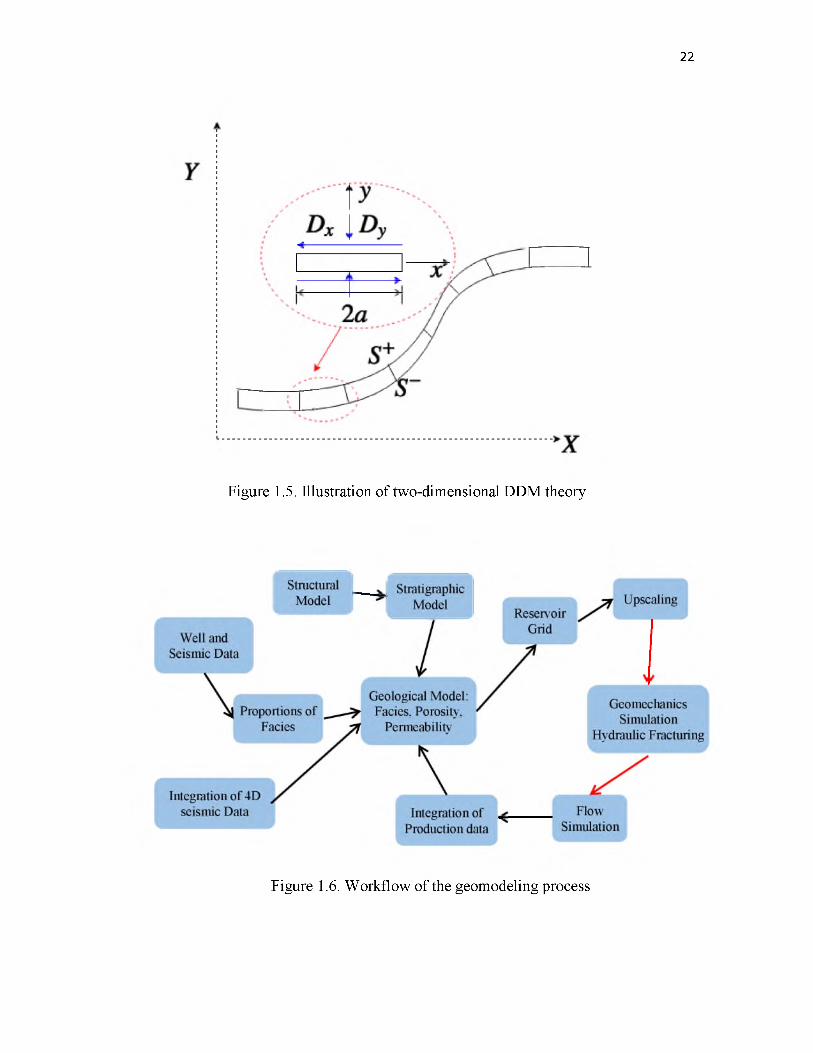
Reservoir exploration is a complex process which integrates a variety of disciplines,

including but not limited to geology, petrophysics, geostatistics, geomechanics, and

reservoir engineering, as shown in Figure 1.6. In conventional reservoir exploration

modeling, a geological model is constructed from structural modeling and stratigraphic

modeling based on well log data, core data, seismic data, and other types of field data. The

reservoir grid and properties obtained from the geological model are then entered into a

reservoir flow simulator to predict production. Taking into consideration the limited

information about the reservoir and the ineffective data interpretation, the geological model

has some uncertainty. By assimilating field production data into the numerical model, the

geological properties, including permeability and porosity, can be calibrated to match the

production data and reduce the uncertainty. However, for unconventional formations, the

geomodeling process contains another important step before the flow simulation:

geomechanics modeling due to the low permeability of formation and the requirements for

hydraulic fracturing.

My research focuses on developing an integrated workflow of incorporating

18

geomechanical hydraulic fracture generation, the depletion of hydrocarbon based on

realistic nonplanar fracture, and model parameter estimation using the Ensemble Kalman

Filter (EnKF). The specific objectives of my research are to:

(1) Investigate the induced hydraulic fractures’ geometry in both homogeneous and

heterogeneous reservoirs based on a novel dual-lattice, fully coupled, hydro­

mechanical hydraulic fracture simulator.

(2) Analyze the mechanical interactions between multiple fractures and study different

factors which will impact the hydraulic fractures’ pattern, including in-situ stress

anisotropy, perforation cluster spacing, treatment of wellbore, and injection

viscosity and rate.

(3) Examine the performance when hydraulic fractures intercept single/multiple

natural fractures (NFs). The influences of hydraulic fractures’ approaching angle,

in-situ stress, natural fracture properties, and injection properties on facilitating the

formation of complex fracture networks will be investigated.

(4) Apply this hydraulic fracture simulator to realistic layered heterogeneous

unconventional reservoirs, and optimize well-completion strategy.

(5) Integrate the realistic fracture geometry with a flow simulator to estimate pressure

distribution and hydrocarbon recovery, which is expected to give some insights in

improving the production from shale formation.

(6) Assimilate the production data to calibrate the geological reservoir parameters and

reduce the uncertainty. The reservoir heterogeneity and fracture characteristics will

be validated through the Ensemble Kalman Filter.

In this dissertation, Chapter 2 discusses the methodology of the novel hydraulic

19

fracturing simulator based on the quasistatic discrete element method. Hydraulic fractures’

propagation in homogeneous and heterogeneous reservoirs will be described in Chapters 3

and 4, respectively. The interaction between hydraulic fracture and natural fracture is

illustrated in Chapter 5. Chapter 6 gives the hydrocarbon production profile with the

realistic nonplanar hydraulic fractures. The algorithm of calibrating and updating reservoir

parameters using the Ensemble Kalman Filter will be discussed in Chapter 7. Finally, a

summary of this research and some suggested further work are discussed in Chapter 8.

20

Figure 1.1. U.S. net energy imports from 2005 to 2040 in six cases (U.S. Energy Information Administration, 2015 Annual Energy Outlook)

2012 Projections

Natural gas

Renewables

Crude oil and 22% natural gas plant liquids

Nuclear

1980 1990 2000 2010 2020 2030 2040

Figure 1.2. U.S. energy production by fuel, 1980-2040 (quadrillion Btu) (U.S. Energy Information Administration, 2014 Annual Energy Outlook)

21

Figure 1.3. Induced curving hydraulic fractures due to mechanical interactions

Figure 1.4. Possible induced fracture pattern in naturally fractured reservoir (red lines represent natural fractures, the blue line is induced fracture pattern)

22

Figure 1.5. Illustration of two-dimensional DDM theory

Figure 1.6. Workflow of the geomodeling process

C H A PT E R 2

HYDRAULIC FRACTURE SIMULATOR

In this chapter, a complex hydraulic fracture propagation model is developed based on

the Discrete Element Method (DEM). After being introduced into the rock-mechanics

problem by Cundall [73], DEM has been widely applied in solving unconventional

reservoir geomechanics problems, such as hydraulic fracture propagation and proppant

transportation. It is used to model the mechanical deformation and fracturing of

polycrystalline rocks at various scales in the geotechnical engineering community, ranging

from grain-scale microcracks to large-scale faults associated with earthquakes.

The model proposed in this chapter fully couples geomechanics and flow. In Section

2.2, the generation of both DEM lattice and conjugated flow lattice are described in detail.

Section 2.3 introduces the assumptions used in this research from rock mechanics and fluid

mechanics aspects. The comprehensive algorithms, including mechanical interaction, fluid

flow, and coupling strategy, are explained in Section 2.4. Section 2.5 gives the advantages

of dual-lattice DEM in predicting the hydraulic fractures’ propagation compared with other

numerical methods.

2.1 Introduction

Hydraulic fracturing is a very complex process, not only because of the varying

composition of subsurface structure, but also because of the changing of stress with the

opening of hydraulic fractures. The base knowledge of hydraulic fracturing initially comes

from in-door experiments and field studies [16]. The experiments had been done with

different sizes of samples, ranging from small-scale rock sample to large rocks. One

prominent advantage of the laboratory studies is the capability of controlling both the stress

condition and rock structure within artificial samples. Therefore, the induced hydraulic

fracture pattern will be easily observed and the qualitative analysis about the parameters’

impact on the fracture will be more clearly obtained [74], [75]. Field study is much more

complex because of the uniqueness of geological heterogeneity and varying in-situ stress,

which cannot be reproduced in the lab. Johnson and Greenstreet [76] used historical

production data such as bottom hole pressure to estimate the fracturing process. Scott et al.

[77] used sonic anisotropy and radioactive tracer logs to analyze hydraulic fracture

geometry.

Computational modeling has been proven to be an effective tool for analyzing the

fundamental mechanism and optimizing stimulations. The DEM model proposed in this

chapter is used to describe the microcrack initiation and coalescence induced by shear and

normal force and the mechanical interaction between fractures. The fluid flow along the

hydraulic fractures and leakoff from the horizontal wellbore into the formation is simulated

through Darcy’s law. In order to realize the explicit coupling of those two complex

processes, a novel dual-lattice system is proposed. This coupled process is numerically

solved by the sequential iterations procedure.

24

2.2 Dual Lattices

DEM is a mesh-free, discontinuous method. In this method, rock is treated as a granular

material and discretized into a series of densely packed small volumes with finite mass.

Therefore, in our model, a large amount of rock particles are generated first to represent

rock mass. Then those particles will be connected according to their relative distance;

meanwhile a bond will be assigned to each pair of those particles, which actually forms the

first type of lattice — DEM Lattice. Then the conjugated flow lattice will be constructed

based on the DEM network. The DEM lattice is used to simulate the mechanics of fracture

propagations and interactions, while the conjugate irregular flow lattice is used to calculate

fluid flow in both fractures and formation.

2.2.1 Rock DEM Lattice Genesis Procedure

In our DEM model, the DEM lattice is illustrated by Figure 2.1. Rock is represented

by a collection of randomly generated, nonuniform-sized circular rigid particles that may

be joined by elastic beams. If the relative distance between two particles is less than a

critical value (user defined), a beam will be inserted. The DEM lattice-generation process

should ensure that the domain is densely packing and particles are well connected. The size

and distribution of rock particles is arbitrary, but all particles will behave homogeneously

and isotropically at the macroscale. Since the fracture initiation and propagation is

mimicked by bond breakage, the generation and placement of particles actually play an

important role in determining the hydraulic fracture pattern. The material-genesis

procedure employs the following steps:

25

2.2.1.1 Initial Packing

A two-dimensional arbitrary container with a frictionless wall is created initially. Rock

particles are generated randomly and placed into the container arbitrarily. The particles’

diameters satisfy uniform particle size distribution with a predefined average size (Dave)

and bounded by Dmin and Dmax. To ensure an initial packing with reasonable density, we

introduced a reduce factor (Rd) to shrink the size of particles and to increase the total

number of created particles at the initial packing. So the initial particles will be generated

according to a reduced particle diameter Dm (Dm = Dave x Rd). The choice of reduce factor

must take into consideration about the particle expansion in the next generation step, which

means it should be neither too large nor too small. If this parameter is too small, the number

of particles will be so big that severe overlapping will occur. On the contrary, if it is too

large, the particles cannot fully occupy the domain, which will also cause bias in the

mechanical calculation. In my research, we use 0.625 as the reduce factor. The most

essential rule of placing those particles is that no overlapping between particles is allowed

in the generation. The initial particle distribution is shown in Figure 2.2.

2.2.1.2 Dense Packing

It can be seen from Figure 2.2 that there are still many interspaces in the domain that

are not occupied by particles because of the nonoverlapping rule. Generally, after the first

initial packing step, the porosity of the domain (~30% - 40%) far exceeds the desired value.

Therefore, at this step, each particle will be resized back to the original determined value

by dividing the reduce factor. All particles will be increased the same amount, according

to the specific reduction factor. The distribution of adjusted particles can be seen in Figure

26

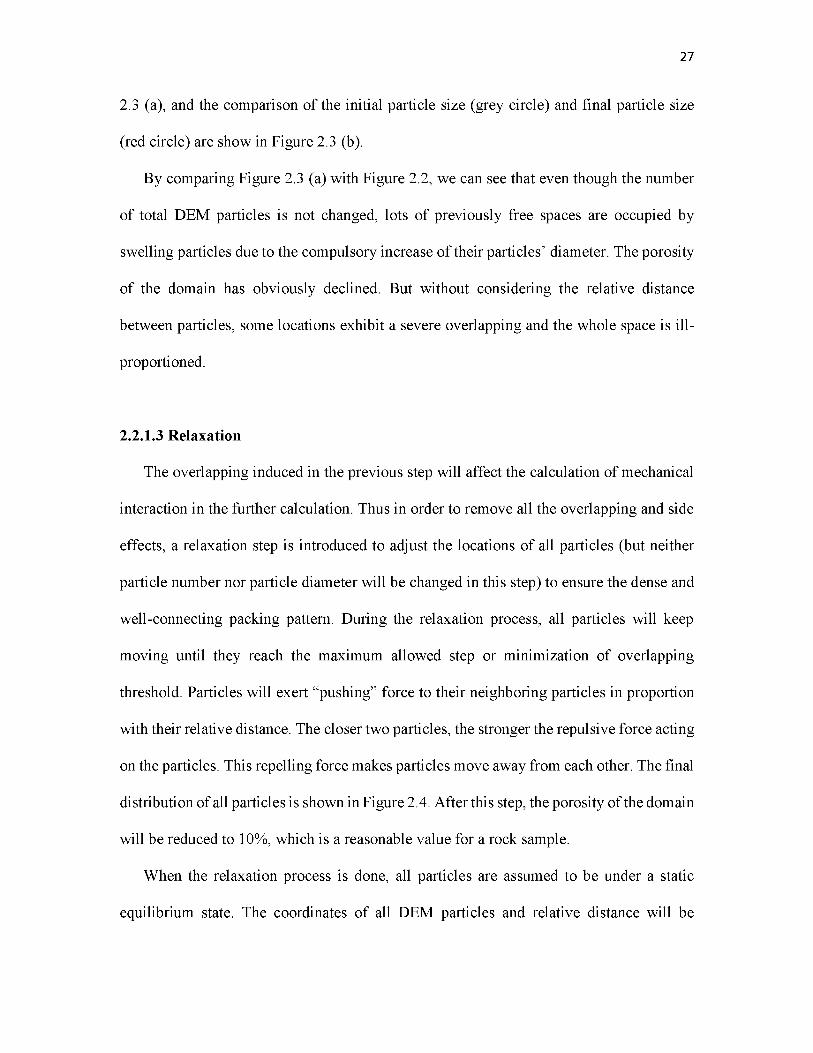
2.3 (a), and the comparison of the initial particle size (grey circle) and final particle size

(red circle) are show in Figure 2.3 (b).

By comparing Figure 2.3 (a) with Figure 2.2, we can see that even though the number

of total DEM particles is not changed, lots of previously free spaces are occupied by

swelling particles due to the compulsory increase of their particles’ diameter. The porosity

of the domain has obviously declined. But without considering the relative distance

between particles, some locations exhibit a severe overlapping and the whole space is ill-

proportioned.

2.2.1.3 Relaxation

The overlapping induced in the previous step will affect the calculation of mechanical

interaction in the further calculation. Thus in order to remove all the overlapping and side

effects, a relaxation step is introduced to adjust the locations of all particles (but neither

particle number nor particle diameter will be changed in this step) to ensure the dense and

well-connecting packing pattern. During the relaxation process, all particles will keep

moving until they reach the maximum allowed step or minimization of overlapping

threshold. Particles will exert “pushing” force to their neighboring particles in proportion

with their relative distance. The closer two particles, the stronger the repulsive force acting

on the particles. This repelling force makes particles move away from each other. The final

distribution of all particles is shown in Figure 2.4. After this step, the porosity of the domain

will be reduced to 10%, which is a reasonable value for a rock sample.

When the relaxation process is done, all particles are assumed to be under a static

equilibrium state. The coordinates of all DEM particles and relative distance will be

27

28

recorded as a reference condition.

2.2.1.4 Installation of DEM Beams

After finalizing the initial packing of all DEM particles, beams are inserted to connect

two particles that are in near proximity (the relative distance between particles has to be

less than 0.25 times the total radius of the two particles). All the beams have been assigned

different properties, including critical tensile strain and critical rotational angle that satisfy

a Gaussian distribution with predefined mean value and variance. Those properties will be

calibrated to match and reflect the material strength that can be obtained through laboratory

experiments or other methods. The calibration process can be found in Huang and Mattson

[78]. The DEM domain with installed beams is shown in Figure 2.5.

The DEM lattice genesis procedure is completed after beam establishment. At this step,

the initial stress has not been applied yet. The mechanical behavior of rock material is

mimicked by the movements (displacement and rotation) of particles and the status of

jointed beams. With the applied load, the beam between two particles will sustain

increasing force that may lead to bond breakage and form microcracks. Continuing with

the load, those microcracks may coalesce and become macroscopic fractures.

2.2.2 Conjugate Flow Lattice-Genesis Procedure

In order to fully couple geomechanics and flow, a conjugate flow lattice is constructed

based on the previous DEM lattice. As mentioned in the last section, the rock is represented

by an assembly of small circular/spherical particles. Due to the shape of DEM particles,

the domain cannot be fully filled with only rock grains, and some blank spaces appear to

exist among particles. Those spaces can be treated as small “reservoirs” that allow the fluid

to be transported. One single conjugate flow node has been assigned to each small

reservoir. Therefore the conjugate flow lattice is generated by connecting all those small

reservoirs and conjugated nodes to provide possible channels for the fluid flow. The DEM

mechanical lattice coupled with the conjugated flow lattice are shown in Figure 2.6.

Since the locations of DEM particles vary with the random number, and the distribution

of conjugate flow node is determined by the DEM lattice, both DEM lattice and conjugate

flow lattice are irregular and will be different if the random number of seed is changed.

Considering that the generation of hydraulic fracture is mimicked by the beam/bond

breakage, the pattern of generated hydraulic fracture will be slightly different because of

different DEM/flow lattices. However, at the macroscale, the statistics, such as average

fracture length, orientation and fracturing pattern, would be almost identical from one

realization to another. The randomness introduced in this dual-lattice system actually

reflects the actual subsurface situation. From a practical point of view, it is impossible to

expect a perfectly homogeneous rock formation.

2.3 The Assumptions Made in our DEM Model

Here are the assumptions made in our hydro-geomechanical hydraulic fracture

propagation simulator based on the DEM method:

For rock mechanics:

1. Hydraulic fracture is required in ultra-low permeable unconventional reservoir

(tight oil or shale gas), and the rock is assumed to be linear elastic material.

2. The DEM particles are rigid, circular (two-dimensional) or spherical (three-

29

dimensional) grain with finite mass.

3. All DEM particles cannot deform or break. However, the overlapping of particles

is allowed during the particle relaxation process. The amount of overlapping is

small compared with the particle radius. And the deformation of this packed-

particle system can be partly described through the particles overlapping.

4. A bond/beam can only be allowed to connect two DEM particles, but not for all

neighboring bodies. The distance between two particles has to be less than a

predefined critical value to form a bond.

5. Each DEM particle has finite displacements and rotations independently.

6. Once the bond between two particles is broken, it cannot recover.

For fluid mechanics:

1. The injection fluid is incompressible.

2. The proppant transportation is not directly included in the research.

3. Fluid flow in the fracture and leakoff into the formation obey Darcy’s Law.

2.4 The Algorithm of Fracture Propagation Based on Dual-Lattice DEM

As mentioned in the previous section, in geomechanical application, the rock is treated

as a granular material jointed together, in which the beams/bonds are breakable with

specific strength [70]. As shown in the enlarged system picture, Figure 2.7, the white lattice

represents the DEM network, and the blue lattice is the flow lattice.

After completing the procedure of generating both lattices, the far field in-situ stress

will be applied to the domain by adding a certain amount of displacements to the

boundaries that will therefore act on all particles. The amount of the displacement (d) can

30

be obtained through

In — s i tu s t ressd = -------------------------

Young 's Modulus

Considering the stress difference in the principal horizontal directions, the added

displacement will be slightly different. After shifting all particles in one direction, particles

will become more densely packed. The overlapping between particles and walls is

indispensable, and may be severe if the horizontal/vertical stress value is large. Thus a

relaxation step is required after installation of in-situ stress to reduce the particles

overlapping and ensure a more uniform particle distribution. After relaxation, we assume

that the whole domain is under a state of equilibrium in which all the particles carried a

specified anisotropic stress and their internal forces balanced initially.

Unlike other DEM-based fracture simulators, such as PFC2D or PFC3D (Itasca, Inc),

which mimic the dynamic process, the current simulator treats fracture propagation as a

quasistatic process wherein the particles keep moving until a stress equilibrium is achieved

for each time step. Attaining equilibrium in each time step is an important assumption made

in the algorithm employed. This assumption is reasonable, taking into consideration the

fact that fluid leakoff and transport rate are much slower compared to force transmission

and fracture propagation.

The forces of all stressed particles can be obtained by tracing the movements of

individual particles and their relative distances. In a DEM model with confined volume,

movements of particles will result from the propagation disturbance caused by the

formation boundary, neighboring particles’ motion, external applied forces, and body

forces. The resultant displacements and rotations of all DEM particles are determined by

both force magnitude and particle properties.

31

After considering all different mechanisms and the existence of beams, the

displacement and rotation of each DEM particle may result from the combined effects from

the following forces, leading to the formation of hydraulic fractures:

1. External force caused by the fluid injection and pressure gradient.

2. Beam force and moment from the beam-connected particles.

3. Viscous damping force.

4. The interaction with neighboring particles which do not have beam connection

initially.

5. The interaction between particles and walls.

6. The stress gradient if the stress is not uniform in the principal directions.

Figure 2.8 depicts the calculation steps used in the model. Since this method is

quasistatic, the dynamic step of calculating particle velocity and acceleration is not required.

Force-Displacement law is used to determine both the translational and rotational motion

of each particle and the contact forces after particle displacement.

Among all those possible forces, pressure gradient is the primary factor leading the

unbalanced force. In Section 2.3.1, all forces except pressure gradient will be discussed in

more detail. The pressure change will be discussed in Section 2.3.2. The force-

displacement law is used to calculate the translational and rotational motion of each particle

from the force.

2.4.1 Geomechanics Calculation

Figure 2.9 gives an illustration of a small piece of rock at the right bottom corner of the

domain. The black vertical and horizontal lines explicitly describe the domain

32

boundaries/walls. With the intrinsic randomness introduced in the algorithm, the particles

vary in both diameters and locations.

Due to the large number of DEM particles and the need of improving the computational

efficient, our model does not consider the impacts from all particles in calculating each

particle’s force or moment. We assume that only neighboring particles will directly affect

the centering particle, and will ignore other particles’ influences. The domain is separated

into many small square boxes of fixed length. The partition of the domain filled with

particles is shown in Figure 2.10, in which the blue dotted line represents box interface.

Each particle is assigned to a specific box, according to its center coordinates. If we define

one particle as belonging to one box, that does not mean this particle is totally embedded

in this box, only the center of the particle is located in the box. The length of the box equals

the diameter of the largest generated particle (Lbox = 2 x Rmax). Thus, each box usually

contains one or two particles.

In Figure 2.10, each particle will be numbered (such as P1~P20) according to its

generation sequence, also all boxes will be labeled (b1~b20). Each box may contain two

particles, at maximum. In the simulator, to reduce the computational load, the force of each

particle will only consider the particle influence from both the assigned box and the

neighboring eight boxes. Take P7 as an example. P7 belongs to the box b7, so in order to

calculate the total force applied on this particle, we have to consider the particles’ influence

from boxes b1, b2, b3, b6, b7, b8, b11, b12 and b13, which include particles P1, P2, P3,

P6, P8, P11, P12, P13 and P14. Therefore, the total particle-particle forces and interactions

for P7 will come from:

i. Beam-connected particle-particle interaction: P2, P6, P8 and P12.

33

ii. Nonconnected neighboring particle-particle interaction: P1, P3, P11, P13 and P14.

At each time step, the definition and location of boxes remains the same, however, the

particles of each box may change due to the particle displacement and rotation. Thus, the

affecting particles should be re-examined every time. The affected zone/blocks can be

enlarged to incorporate more particle interaction at the expense of more relaxation steps

and larger computational load. In the following section, the calculation of all different

forces will be described. In the mechanical calculation, we assume that the deformation of

the individual particles is negligible compared with the deformation of the whole assembly

of DEM particles. The whole domain’s deformation is primarily due to the movement and

rotation of all particles.

2.4.1.1 Beam Force

As described in Section 2.1.1, after the initial packing, if the relative distance between

two particles is smaller than the predefined threshold value, a beam will be inserted to

connect two nearby DEM particles. The beam is used to approximate the mechanical

behavior of elastic brittle cemented rock particles. The beam can transmit both force and

moment between particles and can bend and twist (3 Dimensional) according to the

movement of connected particles. The diagram of beam force is shown in Figure 2.11.

The total force carried by the beam, , contains normal and shear force components

= P u ”iJ + f& s ,j (2.1)

where F-j and Ffj are the normal and shear force. rij, y and Sj, y are the unit vectors parallel

and perpendicular to the center line connecting nodes i and j . When the beam is formed,

we assume that the whole domain is in a state of equilibrium, therefore both force, Fj,y, and

34

35

moment, Mtij , are set to zero initially. The bar over the letters represents that this

property/component is carried by a beam.

The fluid injection and mechanical interaction with surrounding particles will result in

particle movement and rotation. This relative displacement and rotation increment will

produce an increase of elastic force and moment. Therefore, the normal and shear forces

at current time, tn+1, are obtained:

(x ,y ) j l is the distance between the centers of two DEM nodes (the centers of the

corresponding particles), i and j , and d 0j = rt + rj is the initial equilibrium (stress free)

The total normal and shear forces have to project into the x- andy- directions, which

therefore can be used to determine the particle movement in the current time step. So the

forces in both the x- and y- directions can be written as:

(2.2)

(2.3)

where the increments of normal and shear forces are given by

(2.4)

(2.5)

here k n and ks are beam normal and shear stiffness per unit area. d tj = l(x,y)i

distance, where rt is the radius of the i th particle. Qij is the rotation angle in the local

frame of the beam. A is the area of the beam cross-section, which can be calculated by:

(rt + rj)t, t = 1 Two — Dimensional S im ula tor (Vi + m 2

■ I •* I I / i / i / l » 'W i /-i/v-i n » *-\ 'V i /nr / C » ■ w i <i i / /nr * -\'Three — Dimensional S im ula tor(2.6)

Fx = Fn -u* + Fs - u* (2.7)

Fy = Fn - + Fs • u ys (2.8)

where

u% - The projection of normal force in x direction

U* - The projection of shear force in x direction

- The projection of normal force in y direction

u y - The projection of shear force in y direction.

Assuming the angle between normal force direction, n^j , and the x axis direction is d,

we could calculate this angle based on the two particles’ location:

36

u.yn = s in 9 = Vj — ViV (xj — x i) 2 + (yj —y i) 2

u% = cos 9 =Xj — Xj

V (xj — x i) 2 + (yj —y i) 2

Considering that the shear force direction, S i j , is perpendicular to the normal force

direction, n^j , then

= — u y (2.11)

Us = (2.12)

Substituting Equation (2.9) and (2.10) into Equation (2.7) and (2.8), the forces carried

by the beam in both x- and y- can be written as

Fx = Fn -cos 0 + Fs • ( —s in d ) (2.13)

Fy = Fn - s in 9 + Fs • cos 9 (2.14)

Same as the beam force, the moment carried by the beam set to zero initially. The beam

moment at each time step is

(2.9)

(2.10)

37

M ^ 1 = + AMf j (2.15)

The moment increment at each timestep is given by

# = 12 E0I/G0A d 2 (2.17)

where I is the geometric part of its moment of inertia, Eo is macroscopic Young’s modulus,

Go is macroscopic shear modulus, A is the cross-section area of the elastic beam. The

moment of the beam is used to determine the rotation angle of all DEM particles.

2.4.1.2 Viscous Damping Force

While calculating the total force of each DEM particle, a viscous damping force has to

be applied to each particle. Since the energy in the system is dissipated only through friction

and viscous damping, this force is required in the algorithm of discrete element method to

reach the exact equilibrium state during each time step [68].

The viscous damping force can be treated as a movement retardant, which forces the

particles to stick to the ground and move with difficulty. Therefore, the viscous damping

force, Fd , of the particle i can be calculated through

where p is the constant damping coefficient. The negative sign indicates that this force is

always opposite to the particle movement direction, which keep the particle at the previous

location.

F?x = - P x Ax = - P x (x ti +1 - x - ) (2.18)

F«y = - p x A y = - p x ( y ti +1 - y ti ) (2.19)

2.4.1.3 Particle-Wall Interaction

If the reservoir domain is confined by nearby rocks, we assume that the domain is

surrounded by walls and those walls are hard to move. Therefore, if particles overlap with

walls, they will receive additional repellant force exerted from the walls. According to the

wall location, the interaction forces between wall-particles can be summarized as the

following four types:

(1) Interacting with left wall Xmin (Figure 2.12 (a)): the repellent forces from the wall are

(AFr = Wall jConstant x Ax1{ AFy = 0 (220)

(2) Interacting with right wall Xmax (Figure 2.12 (b)): the repellent forces from the wall are

(AFr = —Wall jConstant x Ax?(AFy = 0 (221)

(3) Interacting with bottom wall ymin (Figure 2.12(c)): the repellent forces from the wall are

(AFX = 0[AFy = Wall jConstant x Ay1 (2 22)

(4) Interacting with top wall y max (Figure 2.12 (d)): the repellent forces from the wall are

(AFX = 0[AFy = —Wall_Constant x Ay? (2 23)

According to the force-displacement law, the magnitude of repellent force is linearly

determined by both the overlapped distance between walls and particles and the wall

constant, which is decided based on the surrounding rock properties. The harder the

neighboring rock, the bigger value the wall constant.

As mentioned previously, after the initial relaxation step, all DEM particles are under

the state equilibrium, the force between particles and walls is zero as well. Thus, the wall-

particle force, Fw, at each time step is only determined by the current overlapped distance

38

39

between particle and wall.

F™ =AFX ,- AFX (2 24) ry = nry

2.4.1.4 Nonconnected Neighboring Particles Interaction

Besides the connected DEM particles, lots of particles are not connected by beams.

There are two possibilities that two neighboring particles do not have beam connection:

1. Particles used to be connected by a beam, which is broken and removed later from

the DEM lattice due to the fluid injection and particle displacement;

2. Initial distance between two particles is larger than the connectivity threshold, thus

no beam is installed between those particles. However, because of particle movement and

rotation, particles may come close enough to form a contact force.

As mentioned in the previous section, the whole domain is separated into many boxes,

and all DEM particles have been assigned to a specific box. Therefore, while searching for

the individual particle-particle interaction force (no beam connection), only the

neighboring eight boxes around this particle, called the interacting zone, will be considered.

The particles that belong to other boxes are assumed to be too far away to bring significant

impact on the particle movements.

Therefore when a particle is located in the interacting zone and no beam is present, a

contact force, Fij , will act on both particles (Figure 2.13), which can be described as:

FUj - Ffiriij + F f J i j (2.25)

Similar to the force carried by beams, the force vector Fij also contains normal force,

F™j, and shear force, F?j , components. n^j and Sij are the unit vectors parallel and

perpendicular to the center line connecting nodes i and j . Different from the beam force

vector, F™j and Ffj can be obtained through:

'F£j = kn (d i j — d 0j )1 (2.26)

Fij = ^ 2 ( @i,j + $j,i)

40

where d itj = l ( x , y ) t — (x, y ) j | is the distance between the centers of two DEM nodes (the

centers of the corresponding particles), i and j , and d f j = r t + rj is the initial equilibrium

(stress free) distance, where ri is the radius of the ith particle. f a is the rotation angle in the

local frame of the beam. kn and ks are the normal and shear force constants of rock particles,

which are given by

1 i k n = ~ (kn + k n)2 (2.27)

ks = ^ ( k ls + k ls )

here k ln, k !n and k ls, k !s are the normal and shear force constant of particle i and j ,

respectively. If a regular square or triangular lattice is used in the simulation, kn and ks are

related to the macroscopic Young’s Modulus, E g, Shear modulus, Gc, and Poisson’s ratio,

v, by

k n = ^ ~ (228)

ks = 12EQl[d2(1 + (p)] (2.29)

Both the normal and shear force will also have to be projected into the x- andy- directions

to obtain the particle-particle interaction forces, Fp , and determine the particle

displacement using the Equation (2.30) and (2.31).

Fx = F™j • cos 6 + Ffj • ( — sin 6) (2.30)

Fy = F™j • sin 6 + Ffj • cos 6 (2.31)

In addition, without a beam, there will be no moment in this interaction, which means

the nonconnected particle-particle interaction will not lead to particle rotation.

2.4.2 Pressure Calculation

After applying the in-situ stress on the simulated reservoir domain, all DEM particles

will experience a relaxation step, move independently according to the stress anisotropy,

and reach an initial equilibrium state. This equilibrium will obtain until fluid starts to be

injected. The injected fluid will change the pressure distribution of the whole domain and

exert additional body force to the DEM particles, which will break the equilibrium state

and cause particle movement and rotation. Among all the forces which caused the

displacement, the pressure gradient brought by the fluid injection is the primary and most

significant one.

Currently, the most widespread hydraulic fracturing simulators are based on DDM. The

DDM model estimates the fluid loss from fracture to formation through a constant leakoff

coefficient and cannot simulate the fluid flow in the formation. The way of considering

fluid flow in this method oversimplifies the problem and ignores any change of pressure in

the formation, which could be very significant by inducing the stress change near the

fracture. In addition, this method cannot deal with heterogeneous reservoirs.

In our DEM simulator, a conjugate flow lattice is introduced to calculate the fluid

leakoff and pressure change crossing the domain. Figure 2.14 represents a small piece of

domain filled with rock particles, DEM mechanical lattice (grey lattice), and conjugate

flow lattice (blue lattice). The DEM network is used to calculate the mechanical interaction

41

between particles, and conjugate flow lattice is used to explicitly simulate the fluid

injection and calculate the pressure gradient.

The generation of conjugate lattice relies on the particle distribution and genesis of

DEM lattice. As shown in Figure 2.14, different beams can form irregular mesh (grey

mesh), and one conjugate node is assigned to each of the DEM mesh. For example, the

quadrilateral grid formed by DEM particles A, B, C and D contains single conjugate node

i. Each beam will correspond to two conjugate nodes on each side of the beam (beam A-D

faces to conjugate nodes i and j). By connecting all conjugate nodes, the flow lattice is

formed, which is also irregular.

In order to illustrate the procedure of calculating the flow pressure and the coupling

process, we take the conjugate node i as an example. Node i is in the center of the DEM

grid <ABCD>. Since each beam will correspond to two conjugate nodes, i has 4 conjugate

node connections (j, k, m and h), as shown in Figure 2.15. Therefore, if the fluid is injected

at node i, it will have four leakoff directions (i ^ j), (i ^ k), (i ^ m), and (i ^ h), and the

flowrate is calculated through Darcy’s law in the model. Each flow path can have different

flow properties, such as permeability, so the poroelastic effect and rock heterogeneity are

directly incorporated in the simulator.

We assume that the simulated rock domain is a dry formation without any hydrocarbon

present. Thus, the injection of fracturing fluid can be treated as a single phase, slightly

compressible fluid flow. Since the treatment time of the hydraulic fracturing procedure is

only from several minutes to a few hours, and the permeability of the unconventional

reservoir is pretty low (on the order of nano darcy), this single-phase assumption is

reasonable. The governing equation for single-phase fluid flow in porous media is

42

43

(2.32)

where 0 is rock porosity, k is permeability, p is fluid density, ^ is fluid viscosity, P is

pressure, v is the fluid velocity tensor, and q is injection rate.

While calculating the pressure at each conjugate node, control volume method (CVM)

is adopted. The CVM is derived from a finite-element point with a focus on explicit

expression for local fluid flux [79]. For the conjugate node i, the control volume used to

solve Darcy’s law is the quadrilateral grid <ABCD>.

The residual function of a control volume cvi with boundary r i can be obtained through

the integration of Equation (2.32):

where n is the unit outward normal on ri. According to the geometry of the control volume,

cvi, the boundary r i contains four parts, AB, BC, CD, and AD . Therefore, the Equation (2.33)

can be written as

where cR is rock compressibility, Cf is fluid compressibility, $ ° is the porosity at reference

pressure P° , p° is the fluid density at reference pressure P° . Therefore, the accumulation

(2.33)

(2.34)

Accumulation Flux Source

Both porosity and fluid density are the function of pressure,

<P~<P0[1 + cR( P - P 0)] (2.35)

p ~ p ° [ l + cf ( P - P 0)] (2.36)

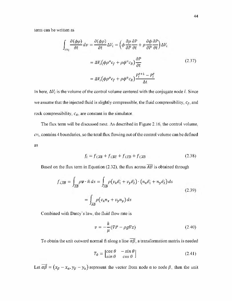
44

term can be written as

f d ((pp) j d ((pp) ATy ( ^ d p d P d(pdP\Jcv. d t V dt 1 V d P d t P d P d t ) 1

= AVi($p°cf + p $ ° c R) ^ (237)

p t + i _pt= AVi(<pp°cf + p<p°cR) 1 ^ 1

In here, AVt is the volume of the control volume centered with the conjugate node i. Since

we assume that the injected fluid is slightly compressible, the fluid compressibility, cy, and

rock compressibility, cR, are constant in the simulator.

The flux term will be discussed next. As described in Figure 2.16, the control volume,

cvi, contains 4 boundaries, so the total flux flowing out of the control volume can be defined

as

fi = fi,AB + fi,BC + fi.CD +fi ,AD (2.38)

Based on the flux term in Equation (2.32), the flux across AB is obtained through

f u n = \ _ p v • f i ds = f p ( v xe1 + vy e2) • (nxei + ny e2) ds'ab 'ab

= I P(VXnX + VyUy) ds J~AR

+ vynyj>AB

Combined with Darcy’s law, the fluid flow rate is

kv = — (VP _ pgVz) (2.40)

To obtain the unit outward normal n along a line a(3, a transformation matrix is needed

rp _ \ c o s 0 —sin 01T e - \ s i n e c o s e l (241)

Let a(3 = (x^ _ xa,yp _ ya) represent the vector from node a to node P; then the unit

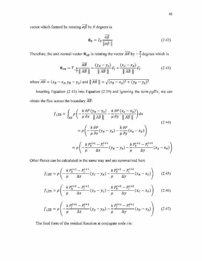
45

vector which formed by rotating a(3 by 6 degrees is

aBn e = T e - ? - (2.42)

I M II

--- » ftTherefore, the unit normal vector nAB is rotating the vector AB by - - degrees which is

AB (y B - Ya) ^ , (xA - xB) ^ ^nAB= T n , ,__, , , = , ,__ ,,, e1 + „ ^ ——e 2 (2.43)-^H AB || II AB II 1 II AB II

where AB = (xB — xA, y B - yA) and I AB I = J (xB - xA) 2 + (y B - y A) 2.

Inserting Equation (2.43) into Equation (2.39) and ignoring the term pgVz, we can

obtain the flux across the boundary AB :

'M t = L p ( - t

____. , k dP (y B - yA) k dP (xA - x ^ \ j

1,AB = Ja bP \ Vd x I AB I ^ d y I AB II ) S(2.44)

. k d P k d Py A ) - ^ d ^ (XA - Xb)

. k P£+1 - Pl+1 k P£+1 - P[+1p ( — H ------ (Vb - Va) - p ^ — (Xa - Xb)

Other fluxes can be calculated in the same way and are summarized here

. k P1+1 - PI+1 k P1+1 - PI+1 . f , M = P \ - -------- ■£,------ (Vc —y B ) — -- ------ ^ ------ (% - Xc) I (245)

b pt + 1 _ pt + 1 b pt + 1 _ pt + 1

f i 'W = P ( - J i h A x ' ( y° - " Ay ' (Xc - Xd) 1 (246)

k p t + 1 -pl^+1 k p t + 1 -p1^ + 1 f i lm = p \ - - — — (yA - vd) - - — — (*d - xA) ) (2.47)

The final form of the residual function at conjugate node i is:

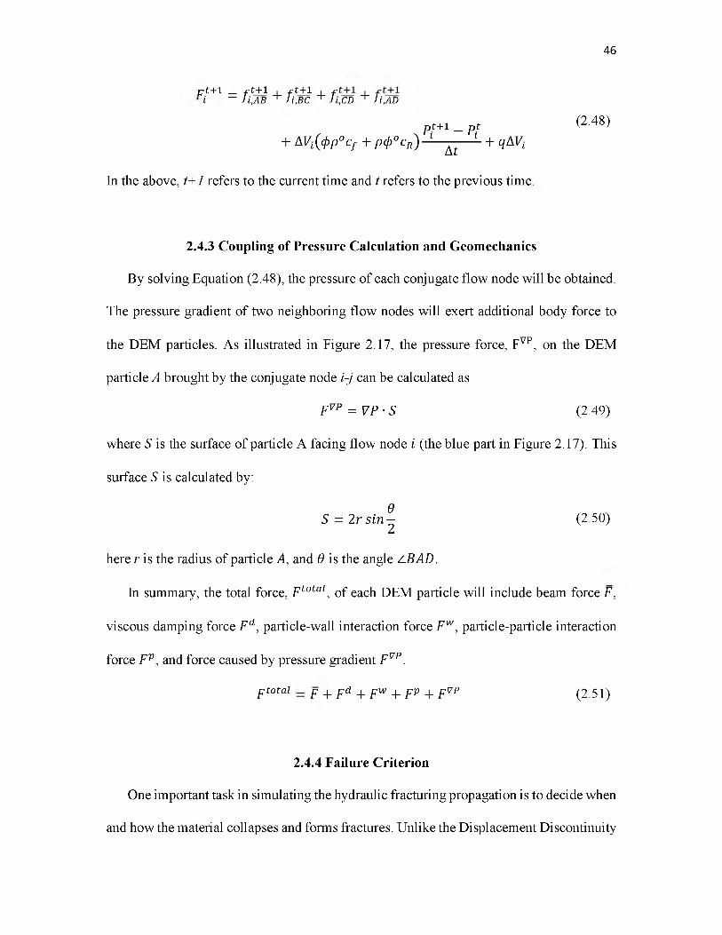
Tjt+l _ f t + 1 ■ f t + 1 ■ f I"i _ li,AB + Ji,BC + Ji,CD + Ji,AD

pt+1 _ pt+ AVi(<pp°cf + p<p°cR) 1 ^ 1 +qAVi

In the above, t+1 refers to the current time and t refers to the previous time

2.4.3 Coupling of Pressure Calculation and Geomechanics

By solving Equation (2.48), the pressure of each conjugate flow node will be obtained.

The pressure gradient of two neighboring flow nodes will exert additional body force to

the DEM particles. As illustrated in Figure 2.17, the pressure force, FVP, on the DEM

particle A brought by the conjugate node i-j can be calculated as

Fvp = VP^S (2.49)

where S is the surface of particle A facing flow node i (the blue part in Figure 2.17). This

surface S is calculated by:

gS = 2 r s i n — (2.50)

2

here r is the radius of particle A, and 6 is the angle a BAD.

In summary, the total force, Ftotal, of each DEM particle will include beam force F,

viscous damping force Fd, particle-wall interaction force Fw, particle-particle interaction

force Fp, and force caused by pressure gradient Fvp.

ptotal = p + pd + pw + p V + pVP (2.51)

2.4.4 Failure Criterion

One important task in simulating the hydraulic fracturing propagation is to decide when

and how the material collapses and forms fractures. Unlike the Displacement Discontinuity

46

(2 .48)

method or analytical model, which obtain the fractures’ propagation direction and length

by calculating the stress intensity factor, our DEM simulator utilizes a more straightforward

and physical-based method to simulate fracture initiation and propagation.

Fracturing process in the DEM simulator is mimicked explicitly by breaking beams

and removing broken bonds from the DEM network. Failure criteria are used to achieve it.

The initiation of new microfractures, as well as the further growth and coalescence of the

microcracks, finally leads to the macroscopic fractures of the formation. This phenomenon

is important in recovering oil and gas from unconventional reservoirs with ultra-low

permeability and porosity, because created fractures provides the primary flow path for the

hydrocarbon from formation to wellbore. Li [80] classified the macroscopic failure criteria

in four categories:

1. Stress or Strain failure.

2. Energy type failure.

3. Damage failure.

4. Empirical failure.

And for brittle material, there are four kinds of classic failure functions:

1. Mohr Coulomb criterion for cohesive-frictional solids.

2. Tresca criterion based on maximum shear stress.

3. Von Mises criterion based on maximum elastic distortional energy criterion.

4. Drucker-Prager criterion for pressure-dependent solids.

In our simulator, the Von Mises failure criterion is used to determine the rock behavior.

If a beam satisfies the Von Mises criterion

47

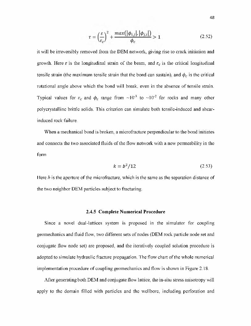
48

(2.52)

it will be irreversibly removed from the DEM network, giving rise to crack initiation and

growth. Here £ is the longitudinal strain of the beam, and £c is the critical longitudinal

tensile strain (the maximum tensile strain that the bond can sustain), and $ c is the critical

rotational angle above which the bond will break, even in the absence of tensile strain.

polycrystalline brittle solids. This criterion can simulate both tensile-induced and shear-

induced rock failure.

When a mechanical bond is broken, a microfracture perpendicular to the bond initiates

and connects the two associated fluids of the flow network with a new permeability in the

form

Here b is the aperture of the microfracture, which is the same as the separation distance of

the two neighbor DEM particles subject to fracturing.

Since a novel dual-lattices system is proposed in the simulator for coupling

geomechanics and fluid flow, two different sets of nodes (DEM rock particle node set and

conjugate flow node set) are proposed, and the iteratively coupled solution procedure is

adopted to simulate hydraulic fracture propagation. The flow chart of the whole numerical

implementation procedure of coupling geomechanics and flow is shown in Figure 2.18.

After generating both DEM and conjugate flow lattice, the in-situ stress anisotropy will

apply to the domain filled with particles and the wellbore, including perforation and

Typical values for ec and $ c range from ~10-3 to ~10-2 for rocks and many other

k = b 2/ 12 (2.53)

2.4.5 Complete Numerical Procedure

injection strategy, will be set up. The simulation of coupled DEM geomechanics and flow

model consists of fluid flow in porous media, mechanical relaxation of the DEM network,

and beam breaking.

During each time step, the nonlinear fluid flow Equation (2.48) is solved first and the

new fluid pressure field will be obtained. Then the updated fluid pressure distribution is

applied to the DEM network according to Equation (2.49), and the DEM network will be

relaxed to a new mechanical equilibrium. Since hydraulic fracture propagation is a

sequential procedure, it is worth noting that only one beam will break at each relaxation

step. The beam that most exceeds the failure criteria, which is usually near a crack tip, is

then removed from the DEM network and the network is again relaxed into a new state of

mechanical equilibrium with the dissipated energy from the broken bond. The mechanical

relaxation and beam breaking are repeated a number of times during each time step,

mimicking crack initiation and propagation, until no additional beam-breaking occurs, and

the simulation proceeds to a new time step.

This quasistatic approach to model hydraulic fracturing is reasonable, since stress

building up and relaxation associated with hydraulic fracture propagations often exhibit

quasistatic behaviors.

2.5 The Advantages of Dual-Lattice Discrete Element Method

Compared with other numerical methods used to predict the hydraulic fracture

propagation process, including Finite Difference/Finite Element Method (FDM/FEM),

Extended Finite Element Method (XFEM), and Boundary Element Method (BEM), our

novel Dual-Lattice Discrete Element Method (DL-DEM) has the following advantages:

49

1. The nature of rock mass is discontinuous, anisotropic, and inhomogeneous [81]. To

adequately represent rock in numerical simulation, the computational model should

be able to capture those features. DEM is a mesh-free discontinuous method

described by discretizing the whole domain into an assembly of particles. The

discontinuity, anisotropy and heterogeneity can be directly incorporated and

reflected in the algorithm through the assignment of different properties to particles.

2. It is a physical-based direct method in describing the rock failure and damage.

Unlike other continuum methods that calculate the irreversible microstructural rock

damage through different constitutive laws and empirical formulations, this direct

method utilizes the breakage of structural beams to represent damage. Therefore, it

is well suited to understand the evolution of damage development and rock rupture.

3. The method can track the loss of beams automatically and it is able to explicitly

represent finite displacement, body rotations, and complete detachment, which is

very difficult to realize for other numerical methods.

4. Because of the proposition of conjugated flow lattice, the fluid flow along the

fracture and leakoff into the formation can be calculated through Darcy’s Law

based on this flow lattice. Therefore the poroelastic effect and fluid leakoff are

fundamentally included. The calculation of geomechanical interaction and

hydraulic fluid injection are explicitly coupled.

5. No prior microfracture is needed. The orientation of induced hydraulic fracture is

fully determined by the stress condition. However, for other methods, in order to

initiate a fracture, an artificial notch should be placed in the domain in advance,

and the fracture propagation will be affected by this prior fracture character.

50

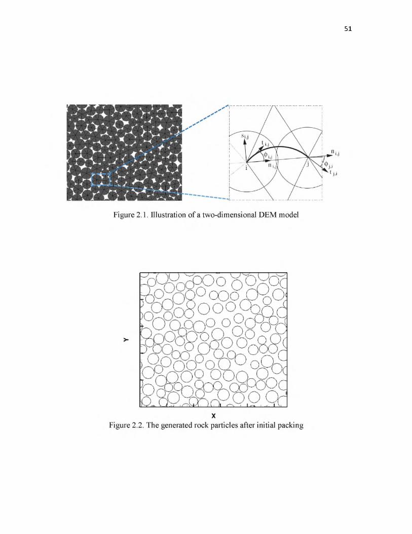
51

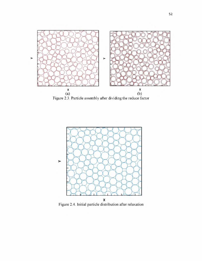
52

(a) (b)Figure 2.3. Particle assembly after dividing the reduce factor

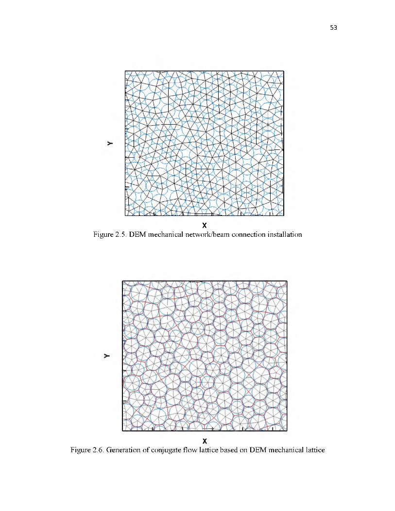
53

XFigure 2.5. DEM mechanical network/beam connection installation

XFigure 2.6. Generation of conjugate flow lattice based on DEM mechanical lattice

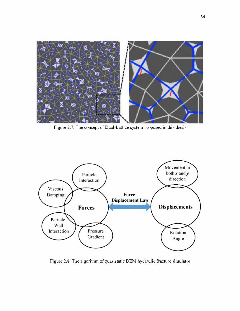
54

Figure 2.7. The concept of Dual-Lattice system proposed in this thesis

Figure 2.8. The algorithm of quasistatic DEM hydraulic fracture simulator

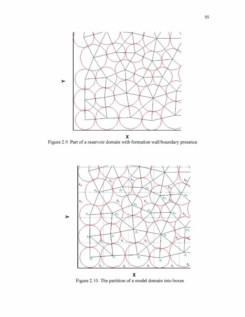
55

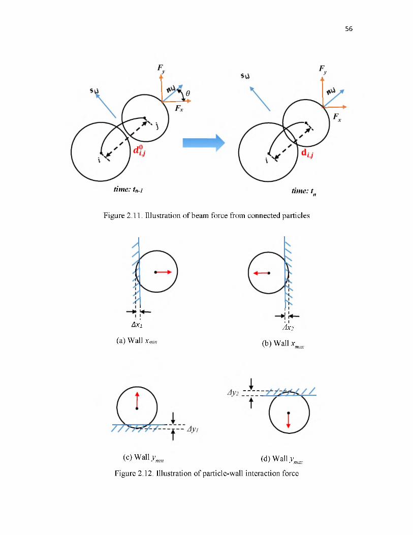
56

time: tn-i time: tn

Figure 2.11. Illustration of beam force from connected particles

Axi

(a) Wall Xm

JX2

(b) Wall x\ / m

(c) Wall y min (cl) Wall y ma:

Figure 2.12. Illustration of particle-wall interaction force

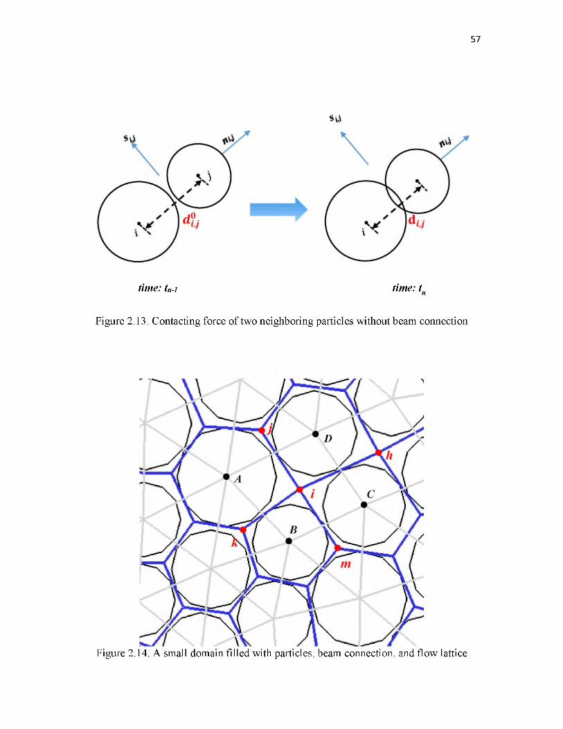
57

time: tn-i time: t

Figure 2.13. Contacting force of two neighboring particles without beam connection

Figure 2.14. A small domain filled with particles, beam connection, and flow lattice

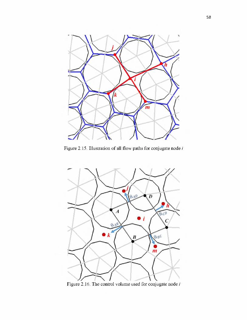
58

Figure 2.15. Illustration of all flow paths for conjugate node i

Figure 2.16. The control volume used for conjugate node i

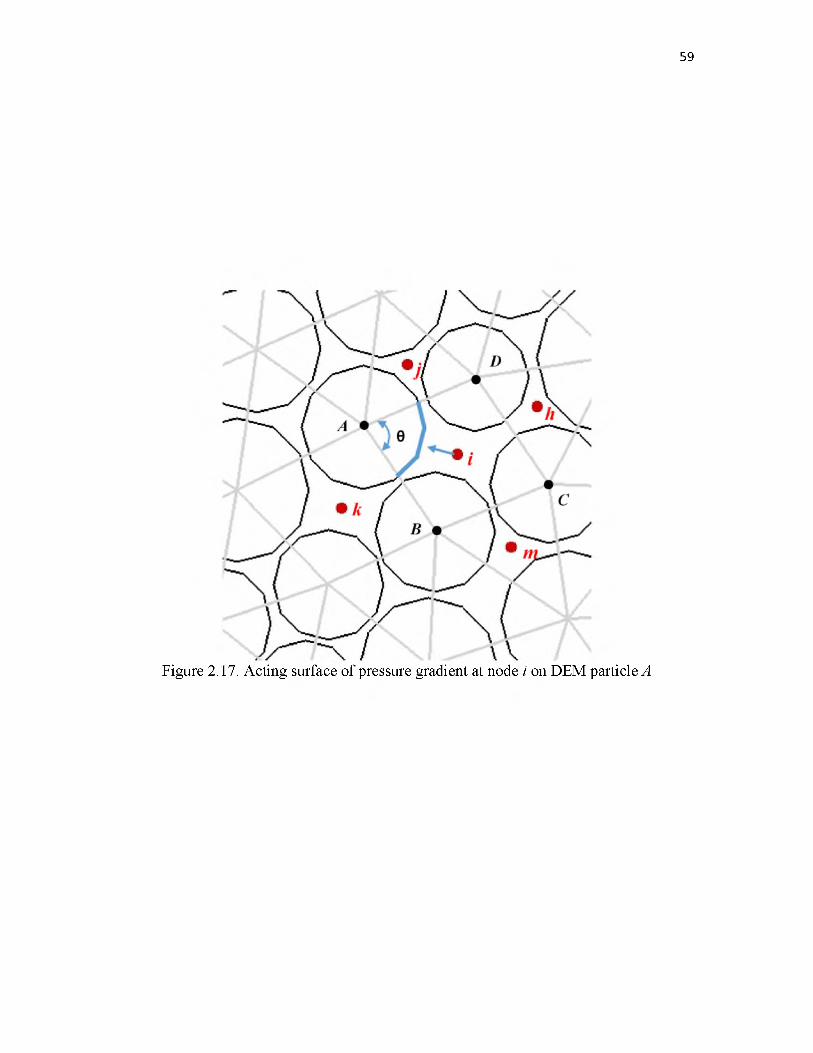
59

Figure 2.17. Acting surface of pressure gradient at node i on DEM particle A

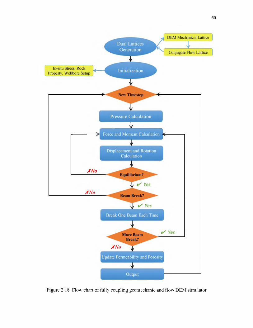
60

Figure 2.18. Flow chart of fully coupling geomechanic and flow DEM simulator

C H A PT E R 3

MULTIPLE HYDRAULIC FRACTURES’ PROPAGATION

IN HOMOGENEOUS RESERVOIR

In Chapter 2, a novel physics-based hydraulic fracturing simulator based on coupling a

quasistatic discrete element model for deformation and fracturing along with a conjugate

lattice network flow model for fluid flow in both fracture and matrix was developed.

Instead of directly using conventional macroscopic rock mechanics parameters, including

Young’s modulus and Poisson’s ratio, the DEM model utilizes different sets of parameters,

such as normal/shear force constants and critical normal/shear strain.

In this chapter, this fully coupled geomechanics and flow hydraulic fracturing simulator

is used to simulate multiple nonplanar fractures’ propagation from a horizontal wellbore in

a homogeneous unconventional reservoir. The effects of geological parameters, such as in-

situ stress, as well as the controllable operational parameters, including perforation

spacing, injection properties, and wellbore treatment, will be investigated. The purposes of

those simulations are to demonstrate the important role of mechanical interaction and stress

shadow effect in multiple fracture propagation and provide some insights in optimizing the

completion strategy and improving the estimated ultimate recovery (EUR). The multiple

hydraulic fractures’ propagation from a single wellbore will be discussed in Section 3.1.

The fractures’ interaction from multiple wellbores will be investigated in Section 3.2.

3.1 Hydraulic Fracture Propagation From Single Wellbore

Extensive hydraulic fracturing is required for successful production from shale gas and

tight oil reservoirs, which usually have ultra-low, nanodarcy-range permeability. The

propped hydraulic fracture will provide high conductivity flow path from formation to

wellbore, which can facilitate the recovery of hydrocarbon from subsurface. In order to

maximize oil and gas production, a complex fracture pattern is usually more favorable for

providing more well-connected flow channels.

The conventional methods of predicting hydrocarbon recovery from fractured

unconventional reservoirs are based on the assumption of planar and orthogonal hydraulic

fractures with uniform fracture conductivities. However, due to the existence of stress

shadow and mechanical interaction between generated fractures, the fracture geometry may

be deviated from the bi-wing planar shape and lead to the formation of complex geometry.

Nonplanar fracture propagation may lead to negative influences on fracture operations,

such as extremely high treating pressure [82], [83], reduction of fracture width near

wellbore [84] or proppant screen out. Therefore, understanding that the stress shadow

effect plays an important role in determining the wellbore completion strategies.

In this section, the interactions between hydraulic fractures initiated from the same

wellbore are investigated. To start with, a simple case of two fractures propagating

simultaneously from the same horizontal wellbore are described in Section 3.1.1. The effect

of injection strategies will be examined in Section 3.1.2. Then the model is applied to a

more complex situation with six perforations in one stage in Section 3.1.3. Finally, a series

of sensitivity simulations is conducted to investigate the effects of in-situ stress, rock

property, number of perforations, and fluid viscosity.

62

3.1.1 Two Hydraulic Fractures Propagate Simultaneously

In this example, the fracture interaction and stress shadow effects are illustrated through

a simple case wherein two fractures initiate simultaneously from a single horizontal

wellbore. As shown in Figure 3.1, two fracture clusters initiated from the same horizontal

wellbore, which is along the minimum stress direction. In each fracture cluster, only one

fracture is considered to propagate from multiple perforations. The input parameters of

rock properties and stress conditions are summarized in Table 3.1. The horizontal wellbore

is located at the bottom of the domain. The maximum horizontal stress is oriented in the y-

direction. The simulated result of induced fracture geometry is shown in Figure 3.2.

Figure 3.2 shows that in a homogeneous reservoir, the two induced hydraulic fractures

tend to repel each other during the propagation under the small stress anisotropy. This is

because the opening of a hydraulic fracture will induce additional compressive stresses in

the neighborhood, and therefore push the fractures away from each other, which can be

called a stress shadow effect.

Stress distribution in Figure 3.3 helps to explain and prove this rock behavior. It is

worth mentioning that in this thesis, we use positive value for tension and negative value

for compression. It is obvious that there is a blue/green zone around the hydraulic fractures,

which represents that opening of fractures will squeeze the nearby rock and lead to

accumulation of compressive stress. By comparing the Sxx with Syy in Figure 3.3, both

the affecting area and value of Sxx is much larger than Syy, which proves that the stress

shadow effect will change the components of stress by different amount and thus gradually

move the maximum principal stress direction from y direction to x direction. Since the

fracture path is always trying to propagate perpendicular to minimum local principal stress

63

direction, the fractures’ geometry will become nonplanar and repel each other with certain

curvature.

In addition, another interesting thing can be found in Figure 3.2 is that neither the shape

nor apertures of generated fractures are uniform or symmetrically distributed along the

fracture length (the color represents the fracture aperture). One reason to explain this

phenomenon is that the methodology of DEM is based on a series of randomly generated

particles which are connected by beams. The randomness introduced in the method makes

the generated fractures with varying properties. This randomness makes our model more

realistic and reasonable since unconventional reservoirs are intrinsically heterogeneous.

And those nonsymmetric behaviors cannot be captured by the other numerical methods,

such as DDM.

Next, we are going to examine the effects of spacing and in-situ stress anisotropy on

fracture geometry. Two different spacings (60 f t and 80 ft) and a large stress difference

(Sh ,min/SH,max 0.5) are used. The generated fracture patterns are compared with the

reference case (40 ft, Sh ,min/SH,max 0.9). The results are summarized in Figure 3.4 and

Figure 3.5.

It is obvious from Figure 3.4 that the fractures continue repelling each other in all

spacings if the stress anisotropy is relative small (Sh,min/SH,max = 0.9). The compressive

stress exerted from the opened hydraulic fractures will make fractures grow away from

each other. However, with the increase of spacing between fracture clusters (from 40 f t to

80 ft), the curvature of fractures is decreasing due to the reduction of stress shadow effect.

The far field stress anisotropy tends to overcome this stress shadow effect. As shown

in Figure 3.5, for large stress anisotropy (Sh,min/SH,max = 0.5), the far field stress will

64

65

suppress the stress shadow effect and keep the fracture growing along the far-field

maximum horizontal stress direction so that the fractures are still close to planar geometry.

3.1.2 Two Hydraulic Fractures Propagate Sequentially

In industry, two different injection strategies are used: simultaneous and sequential

fracturing. In simultaneous fracturing process, multiple perforations are injected at the

same time, therefore multiple fractures will be initiated and propagated simultaneously.

However, the sequential fracturing will create fractures one after another while making the

previously generated fracture propped (previous fracture boundary is fixed) [85] or

pressured with fluid (previous fracture boundary is free) [86]. As shown in the previous

section, for the wellbore with two perforations, the fractures will repel each other with

simultaneous injection.

In this section, the effect of sequential injection on induced fracture pattern will be

investigated. The reservoir domain is homogeneous and isotropic. Two perforations are

located at the horizontal wellbore. The perforation on the right will be injected first. After

injecting for 2 minutes, the injection is stopped for about 30 seconds. Then the perforation

on the left will begin to take fracturing fluid. The spacing between the two perforations is

30ft. The rock properties is shown in Table 3.1. The maximum horizontal stress is oriented

in the y -direction.

Two treatment of the first fracture is considered here.

1. Fixed boundary treatment: After the injection stops, the first fracture’s boundary will

be fixed and no movement or displacement is allowed. The subsequent fracture geometry

will not affect the previous fracture shape.

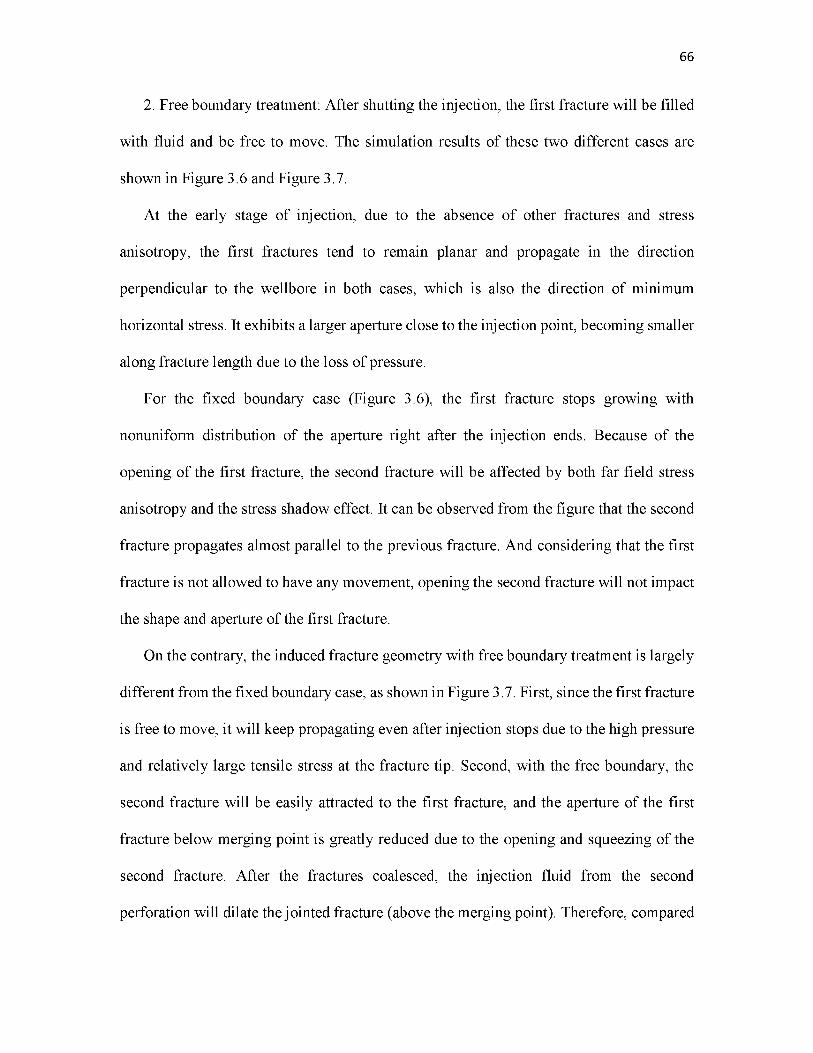
2. Free boundary treatment: After shutting the injection, the first fracture will be filled

with fluid and be free to move. The simulation results of these two different cases are

shown in Figure 3.6 and Figure 3.7.

At the early stage of injection, due to the absence of other fractures and stress

anisotropy, the first fractures tend to remain planar and propagate in the direction

perpendicular to the wellbore in both cases, which is also the direction of minimum

horizontal stress. It exhibits a larger aperture close to the injection point, becoming smaller

along fracture length due to the loss of pressure.

For the fixed boundary case (Figure 3.6), the first fracture stops growing with

nonuniform distribution of the aperture right after the injection ends. Because of the

opening of the first fracture, the second fracture will be affected by both far field stress

anisotropy and the stress shadow effect. It can be observed from the figure that the second

fracture propagates almost parallel to the previous fracture. And considering that the first

fracture is not allowed to have any movement, opening the second fracture will not impact

the shape and aperture of the first fracture.

On the contrary, the induced fracture geometry with free boundary treatment is largely

different from the fixed boundary case, as shown in Figure 3.7. First, since the first fracture

is free to move, it will keep propagating even after injection stops due to the high pressure

and relatively large tensile stress at the fracture tip. Second, with the free boundary, the

second fracture will be easily attracted to the first fracture, and the aperture of the first

fracture below merging point is greatly reduced due to the opening and squeezing of the

second fracture. After the fractures coalesced, the injection fluid from the second

perforation will dilate the jointed fracture (above the merging point). Therefore, compared

66

with the fixed boundary condition which has decreasing aperture from wellbore to

formation, the aperture of the first fracture below merging point (close to the injection

point) is very small, but the aperture above the merging point is large.

The different morphology of the subsequent fracture can be explained by the stress

distributions, as shown in Figure 3.8 and Figure 3.9. Before the generation of the second

fracture, the stress alternation of the domain caused by the opening of the first fracture is

the same in both cases (Figure 3.8(a) and Figure 3.9(a)).

For the fixed boundary case, during the growth of the second fracture, the compressive

stress exerted by the second fracture will accumulate quickly at interval between the two

fractures because of the immovable of the first fracture boundary. Thus the second fracture

will not merge or be attracted to the previous fracture because of this large compressive

stress.

However, for the free boundary condition, since the first fracture is free to move, the

exerted compressive stress from the second fracture will be accommodated by the nearby

rock. There is no significant stress build-up at the interval between the two fractures.

Therefore, the second fracture will be easily attracted to the first fracture.

3.1.3 Multiple Hydraulic Fractures Propagate Simultaneously

In an unconventional reservoir, using closely spaced multiple hydraulic fractures in

combination with horizontal drilling can significantly increase production. During the

completion process of horizontal wells, the reservoir is generally separated into multiple

stages. Each fracture stage usually has three to six perforation clusters which are pumped

and fractured simultaneously. For example, some horizontal wells in Barnett shale have six

67

perforations with equal distance at 50 f t spacing in each stage [87]. As mentioned in the

previous section, opening fractures will induce a stress shadow effect which lead to the

fractures curving and merging. In this section, the interaction between multiple

simultaneous growing fractures will be examined.

The reservoir schematics are shown in Figure 3.10. In this example, we assume that the

reservoir is homogeneous and isotropic, and the model size is 200ft x 200ft. There is a

single horizontal well located at the bottom of the domain. Six perforations are located in

the wellbore, which are equally distributed with spacing of 30ft. The maximum horizontal

stress is oriented in the y -direction and in-situ stress anisotropy is relatively large

(Sh ,min/SH,max 0.5). The injection fluid viscosity is 10 cP and the rate is 50 bbl/min. The

same rock properties are used as shown in Table 3.1.

Since rock particles are randomly generated and distributed, those perforations are not

exactly the same either. Due to the randomness introduced in the algorithm, the geometry

pattern of generated hydraulic fractures will be slightly different among different

realizations. However, at the macroscale, statistics such as total generated fracture

contacting surface and average fracture length would be almost identical from one

simulation to another. Figure 3.11 shows fracture evolution with simultaneous injection.

As the fluid is injected, the pressure in the wellbore begins to build. Once the pressure

at certain perforations is large enough to break the bond of rock particles, fracture will

initialize and start to propagate. Since the pressure loss along the wellbore within one stage

is almost negligible, all perforations will get almost the same fluid initially. However,

because of the randomness of particles’ locations and microproperties, not all perforations

will generate fractures at the very beginning, which can be clearly seen in Figure 3.11(a).

68

This randomness reflects the actual condition of perforations in the subsurface. It is

impossible to expect all perforation-propagating fractures at the same time.

Once the fractures initiate, they will keep growing at a high speed until they reach the

boundary. During this period, other perforations will only have a very small chance to

grow. One of the primary reasons for this phenomenon is the low viscosity of injection.

With low viscosity, the friction loss due to the flow along the fracture is small, thus pressure

at the fracture tip will not experience a dramatic decrease along fracture and will maintain

a sufficient stress to drive the fracture growth. Another important reason is that the opening

of one fracture will exert additional compressive stress near its neighborhood, which

requires larger pressure in the nearby perforations to start the propagation. The value of

induced stress is largely determined by the width and length of the nearby fractures. In

addition, with the opening of a fracture, the permeability of induced fractures will be much

higher than the reservoir formation; therefore, it will take a larger portion of injected fluid

and slow the accumulation of pressure at the wellbore. High breakpoint pressure and low

accumulation rate generally make it difficult to propagate fractures in the other

perforations.

No flow boundary condition for the reservoir is used. Therefore, after fractures get

close to the boundary, they will cease to grow; and the continued injection will widen

induced hydraulic fracture aperture as well as rapidly build up the wellbore pressure, which

allows the generation of fractures from other perforations. It can be seen from Figure 3.11

(c) and (d) that the fracture generated later will be easily attracted to the previously induced

fractures due to the stress shadow effect, which is not favorable in industry due to the

reduction of contacting surface area between the fractures and formation. Therefore, there

69

are only two dominant fractures created in this single stage, which matches the

observations from multifracturing experiments [88], [89].

The observed fracturing pattern can be further explained by the stress field in Figure

3.12. Before the fractures reach boundary, there is a small red zone at the tip of each

perforation/fracture which indicates a large tensile stress concentration. These large tensile

stresses are the primary driving force of fracture opening. A yellow/green zone around the

fractures illustrates that the opening fracture will squeeze the neighboring formation and

increase the nearby compressive stress.

3.1.4 Sensitivity Analysis

In order to maximize the oil and gas production from unconventional reservoirs, it is

preferable to create as much contacting surface between the formation and fracture system

as possible. In the wellbore stimulation, many parameters determine hydraulic fracture

propagation. In this subsection, the impacts of fluid viscosity, rock properties, in-situ stress,

number of perforations, and wellbore treatment on the hydraulic fracture geometry will be

investigated.

3.1.4.1 Effect of Fluid Viscosity

In this subsection, we are going to examine the impact of fluid viscosity on fracture

pattern. Eighty times higher viscous fluid (gel) is used to illustrate the influence of fluid

viscosity, compare with low-viscosity fluid (reference case in Section 3.1.3). The generated

hydraulic fracture patterns are summarized in Figure 3.13.

Unlike low-viscosity cases (Section 3.1.3), fluids with high viscosity will lead to

70

71

multiple fractures’ propagation almost simultaneously at the beginning. The fractures

appear to have much shorter propagated length compared with the low-viscosity fluid

injection (Figure 3.11 (b)). High viscosity will result in much larger fluid pressure loss

along the fracture and then fail to support further fracture growth. The short length of the

fracture will only take a small portion of injection fluid and also reduce the stress shadow

effect on the neighborhood. Therefore, the high wellbore pressure and small stress shadow

will encourage multiple fractures to grow simultaneously.

3.1.4.2 Effect of Rock Properties

The brittleness of the rock is considered next. In order to remove other possible

disturbances to fracture geometry, we use the low-viscosity fluid (10 cP) and the same in-

situ stress anisotropy as shown in Table 3.1 with varying rock properties. For less brittle

rock, smaller Young’s modulus (80% of the original value) but larger critical strain will be

used. Figure 3.14 shows the fracture pattern in a less brittle formation.

With smaller Young’s modulus and larger critical strain, the less brittle rock is harder

to break initially and is able to sustain larger stress. Therefore, at the same initial time,

while the brittle formation has already generated a long fracture (Figure 3.14 (a) tip reaches

nearly 100 ft), a short crack is generated in the less brittle formation. With the injection

continuing, the less brittle formation still exhibits a slower propagation rate.

3.1.4.3 Effect of In-situ Stress Anisotropy

Among all the parameters that impact fracture geometry, stress condition in formation

is recognized as the primary and the most important factor in controlling the fracture’

propagation [90]. The differences in far field principal stress can alter the direction of

hydraulic fractures and determine the shape of induced fractures. In this subsection, we are

going to examine multiple fractures’ propagation under different in-situ stresses.

We still assume that the reservoir is homogeneous and isotropic and the model size is

200ft x 200ft. There is a single horizontal well located at the center of the domain and

oriented with the minimum horizontal stress (Sh,min) direction. Six equally distributed

perforations are located on the wellbore with 30 f t spacing. The maximum horizontal stress

(SH,max) is oriented in the y-direction. Three different initial stress conditions are compared,

Sh ,min/SH,max 0.5, 0.9 and 0.98. To exclude the effects from other parameters, we only

change the value of minimum horizontal stress. The detailed input parameters used are

shown in Table 3.2. Figure 3.15 - 3.17 displays the fracture evolution with time under

different stress conditions.

As in the previous example, some of the perforations will generate fractures after the

injection starts and pressure has accumulated. Comparing Figure 3.15(a) — 3.17(a), at the

early period of fracture propagation (t = 3 min), the case with larger stress difference

(Figure 3.15 (a)) appears to induce longer hydraulic fractures at the early propagation stage.

Because the same maximum horizontal stress is used for all three cases, larger stress

anisotropy (SH,max - Sh,min) indicates smaller minimum horizontal stress. Since one

indispensable requirement for hydraulic fracture propagation is that local stress has to

exceed the minimum horizontal stress, smaller Sh,min is more favorable for fracture growth.

Continuing with the injection, the fractures keep growing. When factures get close to

the boundary, they will cease to grow because of no flow boundary. The opening of a

fracture will exert additional stress and reorient the principal stress direction in the

72

neighborhood, which is known as the stress shadow effect. Since hydraulic fractures favor

minimum principal stress direction, in multiple fracture propagation scenarios, the stress

shadow effect will eventually change the fracture pattern by altering the local principal

stress direction. But the far field stress can help overcome this stress shadow effect. When

the stress difference (SH,max - Sh,min) is very large (Figure 3.15 (b)), the in-situ stress will

suppress the stress shadow and the fractures will remain planar. However, with small stress

anisotropy, fracture propagation is impacted by overprint of additional mechanically

induced stress associated with neighboring fractures, thus the hydraulic fractures will

propagate with no preferential directions.

3.1.4.4 Wellbore Effect: Cemented or Uncemented

A large number of hydraulic fracture papers are attempting to describe the effect of

perforation spacing, in-situ stress condition, fluid viscosity, and flow rate on the induced

fracture geometry. However, only a few papers take into consideration the influence of

wellbore treatment in the fracture pattern from the engineering aspect. Since the cost of

cemented wellbore is higher than uncemented wellbore, a practical question arises: is there

any difference of corresponding fracture patterns from different well completions? In this

part, we are going to compare the hydraulic fractures patterns generated from different

wellbore completion strategies using the numerical simulation results.

In industry, the completion strategies can generally be categorized into: Cemented

liner, Openhole completion, Uncemented preperforated liners. The cemented liner

completion involves cementing the linear through the horizontal wellbore. “Plug-and-perf”

stimulation technique is employed to perforate the pay zone with perforating guns. Then

73

74

the fracturing fluid will be injected through the perforations into the formation to propagate

fractures. Cemented wellbore with perforated casing completion is the most widespread

completion technique nowadays. The main advantage of this completion is that the vertical

well can be drilled through the total depth of production zone. Other benefits of cemented

wellbores include stable borehole, relatively assured locations of fracture initiation,

availability for refracturing, and greater well serviceability.

Both openhole completion and uncemented per-perforated liners’ completions bare

part of the uncemented wellbore. Although not very common in all areas, those wellbores

are still used today in certain situations, such as horizontal well completion in Austin

Chalk. The uncemented wellbore also has many advantages, such as less expense,

favorable production from both well and fracture network, faster depletion of the near

wellbore region. Compared with openhole completion, the uncemented per-perforated liner

completion is capable of controlling fracture initiation and propagation by diverting fluids.

However, those completion strategies have limited applicable situations due to potential

well damage under high pressure or high injection rate.

In low-permeability reservoirs, hydraulic fractures generated from both cemented and

uncemented wellbores are required to provide additional flow path from formation to

wellbore. Whether the generated hydraulic fractures will be different from

cemented/uncemented wellbore plays an important role in determining the well-

completion strategies.

In order to compare the effect of wellbore on the induced hydraulic fracture pattern, we

set up two cases with different wellbore treatmens. Figure 3.18 shows the reservoir domain

and horizontal wellbore used in our numerical simulations. In both cases, the reservoir

domain is homogeneous and isotropic, with a size of 200f t x 200ft. A horizontal wellbore

is located in the center of domain. Usually, the uncemented wellbore does not have

perforations which will lead to randomly initiated hydraulic fractures along the wellbore.

However, in order to exclude the location perturbation on the fracture pattern, we set up

six perforations in both cemented and uncemented wells to ensure the identical

initialization point of fractures. Large stress anisotropy (Sh ,min 0.5 x SH,max) applies to

the domain with the maximum stress direction in the y direction. Other parameters are the

same as the previous section, as summarized in Table 3.1.

For the reservoir with a cemented wellbore (Figure 3.18 (a)), the white area explicitly

represents the horizontal well. The red line along the wellbore explicitly represents

casing/cement, which plays the role of keeping the injection fluid inside the wellbore (no

leakoff from well to formation) and avoiding well expansion or collapse (no movement of

well). For an uncemented wellbore (Figure 3.18 (b)), the horizontal well is also located at

the same place as the cemented well. The main difference is that, after drilling, the injection

fluid will fill in the well and directly contact with the reservoir formation. Therefore,

without cementing, the wellbore is free to move and a small portion of fluid will leak into

the formation according to its permeability. Taking into consideration that fluid has little

resistance to the shearing force but is able to sustain infinite deformation within a confined

environment, we thus assign a small shearing stiffness constant and very large critical

tensile/shear strain to the particles representing the fluid in the wellbore in the simulation.

Figure 3.19 (a) and 3.20 (a) illustrate the hydraulic fracture geometry from cemented

and uncemented wellbore respectively. For both cases, not all perforations will propagate

fractures due to the stress shadow effect. Even though there are small differences between

75

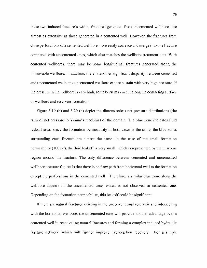
these two induced fracture’s width, fractures generated from uncemented wellbores are

almost as extensive as those generated in a cemented well. However, the fractures from

close perforations of a cemented wellbore more easily coalesce and merge into one fracture

compared with uncemented ones, which also matches the wellbore treatment data. With

cemented wellbores, there may be some longitudinal fractures generated along the

immovable wellbore. In addition, there is another significant disparity between cemented

and uncemented wells: the uncemented wellbore cannot sustain with very high pressure. If

the pressure in the wellbore is very high, some burst may occur along the contacting surface

of wellbore and reservoir formation.

Figure 3.19 (b) and 3.20 (b) depict the dimensionless net pressure distributions (the

ratio of net pressure to Young’s modulus) of the domain. The blue zone indicates fluid

leakoff area. Since the formation permeability in both cases is the same, the blue zones

surrounding each fracture are almost the same. In the case of the small formation

permeability (100 nd), the fluid leakoff is very small, which is represented by the thin blue

region around the fracture. The only difference between cemented and uncemented

wellbore pressure figures is that there is no flow path from horizontal well to the formation

except the perforations in the cemented well. Therefore, a similar blue zone along the

wellbore appears in the uncemented case, which is not observed in cemented one.

Depending on the formation permeability, this leakoff could be significant.

If there are natural fractures existing in the unconventional reservoir and intersecting

with the horizontal wellbore, the uncemented case will provide another advantage over a

cemented well in reactivating natural fractures and forming a complex induced hydraulic

fracture network, which will further improve hydrocarbon recovery. For a simple

76

illustration in Figure 3.21, a homogeneous reservoir has three natural fractures intersected

with the horizontal wellbore. For the cemented one (Figure 3.21 (a)), only one natural

fracture crosses the perforation. On the contrary, the whole uncemented wellbore (Figure

3.21 (b)) is open and directly contacts with all natural fractures. After injecting for a certain

time, the fluid will open and dilate two natural fractures and then continuously generate

hydraulic fractures into the formation in the uncemented open-hole case. However, only

half the length of the natural fracture will reactivate in a cemented wellbore. Fluid is

allowed to leak off from the wellbore into the natural fracture through the openhole

wellbore. Therefore, an uncemented wellbore is much easier to open natural fractures

intersected with a well, and increases the conductivity significantly.

3.2 Hydraulic Fracture Propagation From Multiple Wellbores

Multilateral completion techniques allow the drilling and completion of multiple wells

within a single wellbore. This technique enables the main wellbore to achieve multiple

target zones, and thus increases the stimulated reservoir volume (SRV). In this section, the

potential fracture interactions from multiple laterals will be examined. Consider two

parallel laterals from the same wellbore in a reservoir domain. There are three perforation

clusters in each fracture stage. Due to symmetry, only one fracture stage is simulated here.

The major objective is to investigate the effect of the perforation location on fracture

geometry. In the first case, the clusters are initiated at the same location on each lateral

well, while they are offset from each other in the second case. Both laterals are injected at

the same time. In order to keep the fractures from two laterals propagating toward each

other, we introduce a large initial stress difference (Sh ,min/SH,max 0.5) to compensate the

77

stress shadow effect on the fracture path. In both cases, the maximum stress direction is

along the _y-direction.

Initially, due to the large far-field stress anisotropy, fractures grow with an orthogonal

pattern which is parallel to the maximum stress direction in both cases without obvious

interaction. In the symmetric perforation cluster setting (Figure 3.22(a)), when the fractures

from different wellbores become close to each other, the fractures tend to be attracted by

each other. The cause of this phenomena is mainly due to the induced shear stress around

the fracture tips, which will significantly alter the local stress orientation. However, when

the perforation locations in the two laterals are offset for 100 f t in x-direction (Figure

3.22(b)), there is no obvious attraction between fractures because they are beyond each

other’s stress shadow zone. Under this circumstance, the fractures will keep growing until

they reach the boundary.

The attraction of fracture tip from multilateral wellbores may merge the fractures and

reduce the fracture’s surface area, which generally is not favorable from the perspective of

production. On the contrary, the design with offset well placement will partly relieve the

mechanical interaction between fractures, and thus increase the stimulated reservoir

volume (SRV).

3.3 Summary

The novel dual-lattice, fully coupled hydro-mechanical hydraulic fracture simulator

presented in Chapter 2 is able to simulate the propagation of a hydraulic fracture in

homogeneous reservoirs. The simulator can capture hydraulic fracture propagation, the

mechanical interactions between multiple fractures, and the fluid flow along the fracture

78

and into the formation. In summary, we can conclude that:

1. Stress shadow caused by the opening of fractures will change the orientation of

principal stress in the neighborhood, which will inhibit or alter the growth and

direction of fractures in the nearby perforation clusters.

2. The far-field stress can help overcome the stress shadow effect. Under large stress

anisotropy, the fractures tend to remain planar. The fractures are prone to deflect or

even merge into a single mainstream fracture with low stress anisotropy.

3. In the sequential injection case, the subsequent fracture geometry is determined by

both the stress shadow effect caused by the opened fracture and the treatment of the

previous fractures. If the previous fracture is filled with proppant and hard to move,

the subsequent fractures will propagate in the direction paralleling or moving away

from the previous fracture. However, if the previous fracture is filled with fluid and

free to move, the subsequent fracture will curve toward the previous fracture.

4. Low-viscosity fluid will cause longer but fewer propagated fractures initially. With

the stress shadow and reorientation of principal stress direction, the subsequent

fractures will be attracted and merged into the preceding fracture.

5. The less brittle rock will make it difficult to break and is not favorable for hydraulic

fracturing.

6. Fractures from cemented wellbores more easily coalesce and merge into one

fracture compared with uncemented cases.

7. Fractures generated from uncemented wellbores are almost as extensive as those

generated in cemented wells. However, there are pressure and fluid rate constraints

on the uncemented wellbores.

79

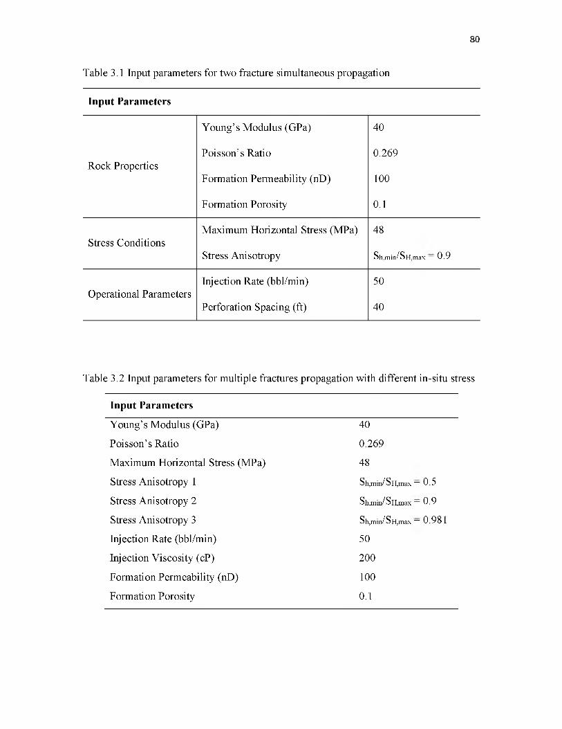
80

Table 3.1 Input parameters for two fracture simultaneous propagation

Input Parameters

Young’s Modulus (GPa) 40

Poisson’s Ratio 0.269Rock Properties

Formation Permeability (nD) 100

Formation Porosity 0.1

Maximum Horizontal Stress (MPa) 48Stress Conditions

Stress Anisotropy Sh,min/SH,max _ 0.9

Injection Rate (bbl/min) 50Operational Parameters

Perforation Spacing (ft) 40

Table 3.2 Input parameters for multiple fractures propagation with different in-situ stress

Input Parameters

Young’s Modulus (GPa) 40

Poisson’s Ratio 0.269

Maximum Horizontal Stress (MPa) 48

Stress Anisotropy 1 Sh,min/SH,max _ 0.5

Stress Anisotropy 2 Sh,min/SH,max _ 0.9

Stress Anisotropy 3 Sh,min/SH,max _ 0.981

Injection Rate (bbl/min) 50

Injection Viscosity (cP) 200

Formation Permeability (nD) 100

Formation Porosity 0.1

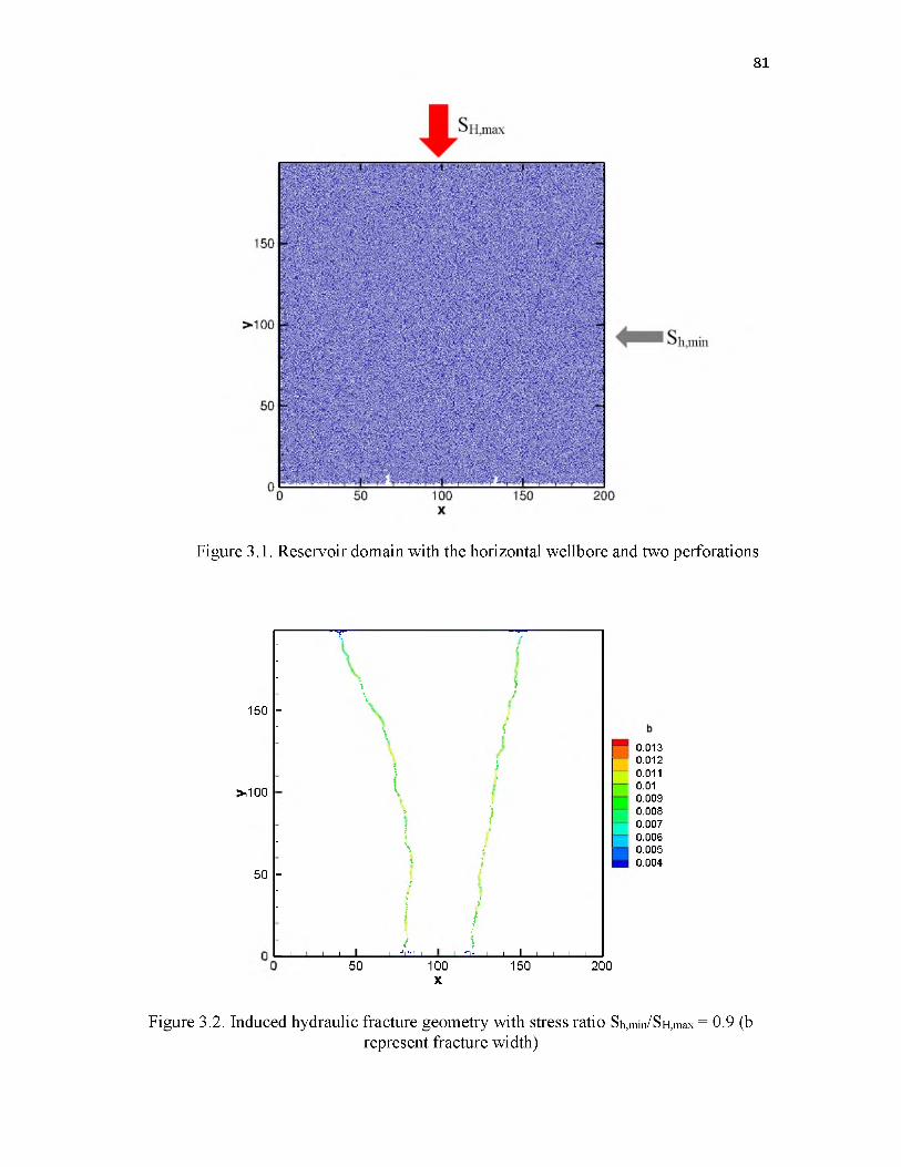
81

Figure 3.1. Reservoir domain with the horizontal wellbore and two perforations

150

>100

50

-T 1

: \ >_ V )

- \ /- if

t

*

- > j\- \ /

-

\

}

ij

-

- Iii

j

-----L___

}i i i i i j r - i

S' i ‘ i i I i i i i

50 100X

150 200

0.0130.0120.0110.010.0090.0080.0070.0060.0050.004

Figure 3.2. Induced hydraulic fracture geometry with stress ratio Sh,min/SH,max = 0.9 (brepresent fracture width)

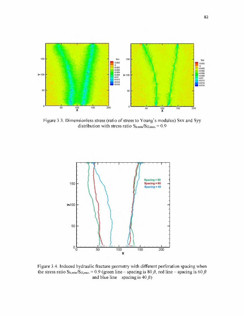
82

Figure 3.3. Dimensionless stress (ratio of stress to Young’s modulus) Sxx and Syy distribution with stress ratio Sh ,min/SH,max 0.9

Figure 3.4. Induced hydraulic fracture geometry with different perforation spacing when the stress ratio Sh ,min/SH,max 0.9 (green line - spacing is 80 ft, red line - spacing is 60 f t

and blue line - spacing is 40 ft)

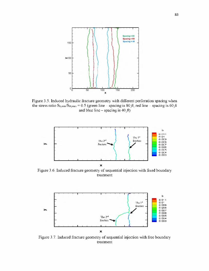
83

Figure 3.5. Induced hydraulic fracture geometry with different perforation spacing when the stress ratio Sh ,min/SH,max 0.5 (green line - spacing is 80 ft, red line - spacing is 60 f t

and blue line - spacing is 40 ft)

n--- 1--- 1--- 1---1-

_i______i_____ i_____ i_____ L

The 2nd fracture

The 1st fracture

b0.01 1

0.010.0090.0080.0070.0060.0050.0040.003

Figure 3.6. Induced fracture geometry of sequential injection with fixed boundarytreatment

“I---1--- 1---1--- 1- i >•

The 1st fracture

— 1_ _ _ _ _ I _ _ _ _ _ I_ _ _ _ _ I_ _ _ _ _ J_

The 2nd fracture '

_ l ____i___ —I______ I______ I_____ i _____I______ I______ L_

0.01 10.010.0090.0080.0070.0060.0050.0040.003

Figure 3.7. Induced fracture geometry of sequential injection with free boundarytreatment

84

(a) Time = 2 minutes (b) Time = 5 minutes

Figure 3.8. Stress distribution Sxx of sequential injection with fixed boundary

(a) Time = 2 minutes (b) Time = 5 minutes

Figure 3.9. Stress distribution Sxx of sequential injection with free boundary

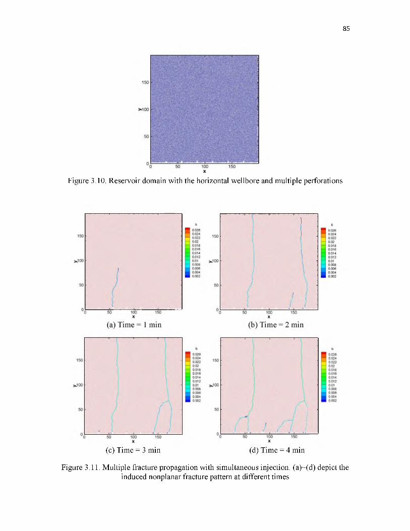
85

Figure 3.10. Reservoir domain with the horizontal wellbore and multiple perforations

(c) Time = 3 min (d) Time = 4 min

Figure 3.11. Multiple fracture propagation with simultaneous injection. (a)~(d) depict the induced nonplanar fracture pattern at different times

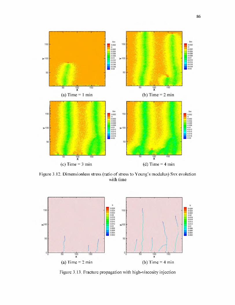
86

(c) Time = 3 min (d) Time = 4 min

Figure 3.12. Dimensionless stress (ratio of stress to Young’s modulus) Sxx evolutionwith time

(a) Time = 2 min (b) Time = 4 min

Figure 3.13. Fracture propagation with high-viscosity injection

87

(c) Time = 3 min (d) Time = 4 min

Figure 3.14. Fracture propagation with less brittle rock. (a)~(d) depict the induced nonplanar fracture pattern at different times

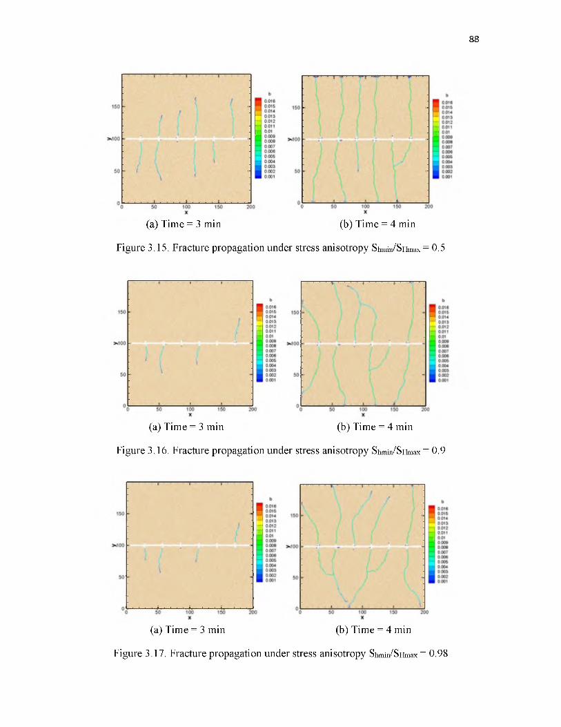
88

(a) Time = 3 min (b) Time = 4 min

Figure 3.15. Fracture propagation under stress anisotropy Shmin/SHmax = 0.5

(a) Time = 3 min (b) Time = 4 min

Figure 3.16. Fracture propagation under stress anisotropy Shmin/SHmax = 0.9

(a) Time = 3 min (b) Time = 4 min

Figure 3.17. Fracture propagation under stress anisotropy Shmin/SHmax = 0.98

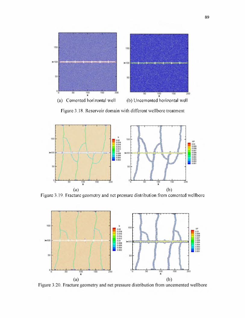
89

(a) Cemented horizontal well (b) Uncemented horizontal well

Figure 3.18. Reservoir domain with different wellbore treatment

(a) (b)Figure 3.19. Fracture geometry and net pressure distribution from cemented wellbore

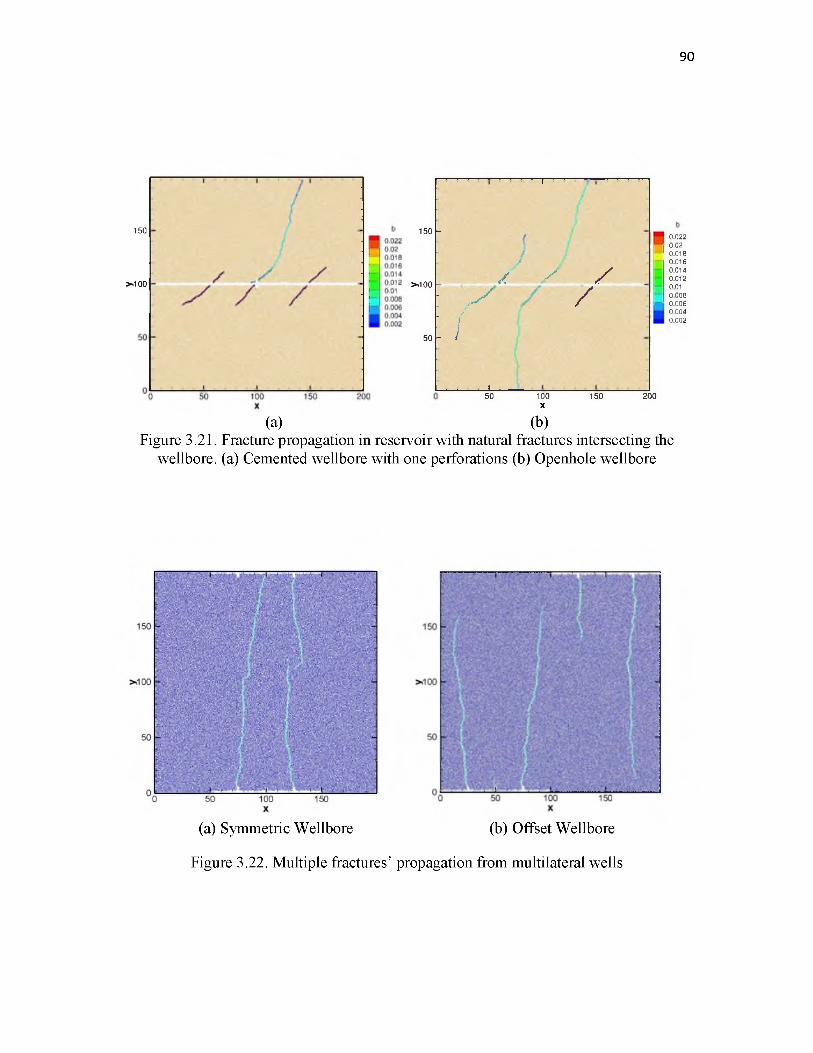
90

150

>•100

150

>100

50

1----

1----

\

-----1---- - ----

, .; ^' /- /

. . . . 1 .

/

50 100X

150 200

0.0220.020.0180.0160.0140.0120.010.0080.0060.0040.002

(a) (b)Figure 3.21. Fracture propagation in reservoir with natural fractures intersecting the

wellbore. (a) Cemented wellbore with one perforations (b) Openhole wellbore

(a) Symmetric Wellbore (b) Offset Wellbore

Figure 3.22. Multiple fractures’ propagation from multilateral wells

C H A PT E R 4

HYDRAULIC FRACTURE PROPAGATION IN

HETEROGENEOUS RESERVOIR

For the sedimentary basin, many reservoirs will be complex, layered, and not

homogeneous. Rock properties and hydraulic parameters such as Young’s modulus,

strength, permeability, and porosity can vary strongly in space due to the movements of

the upper crust of the Earth, including tectonic movements, earthquakes, land

uplifting/subsidence, glaciation cycles, and tides [10], [91]. And these heterogeneities of

reservoir formation will significantly impact the hydraulic fracturing.

In this chapter, we are going to investigate the hydraulic fracture propagation process

in a heterogeneous reservoir also based on the dual-lattice simulator developed in Chapter

2. A simplified heterogeneous model with three layers will be used first to illustrate the

effects of permeability and rock fabric on the fracture geometry. Then this simulator will

be applied to a realistic heterogeneous field. Through the simulation results, we can see

that without considering the intrinsic heterogeneity, the predicted morphology of hydraulic

fractures may be biased and misleading in optimizing the completion strategy.

4.1 Simplified Heterogeneous Model with Three Layers

4.1.1 Permeability Heterogeneity

The reservoir size is 200 f t x 200 ft, with a point source at the center of the domain.

Large stress anisotropy (Sh ,min / SH,max = 0.5) is applied to the domain, with the maximum

stress direction in the y direction. In order to investigate the effect of heterogeneity, the

entire domain contains three layers: the top and bottom layers share the same properties,

which differ from those of the middle layer. To exclude the effects from other parameters,

we only change the permeability of those three layers, while keeping others the same. Four

cases are studied. The middle layer, k, is 100 nd in all cases. The top and bottom layer

permeabilities vary from 100 nd, 10 md, 100 md, to 1 darcy. Input parameters are

summarized in Table 4.1. The generated hydraulic fractures are shown in Figure 4.1.

Figure 4.1 shows that with increasing permeability, the hydraulic fracture exhibits a

gradually reducing propagated length. Especially when the layer’s permeability reaches 1

darcy, the fracture will stop at the layer interface. High permeability will allow more

injection fluid leakoff into the reservoir and result in large pressure loss along the fracture,

therefore there is not enough pressure at the fracture tip to drive its opening.

Figure 4.2 gives the pressure distributions of these four cases. The color map indicates

the dimensionless net pressure value (net pressure/Young’s Modulus). For case (a), with

the same low permeability in all layers (100 nd), the fracture reaches to the boundary very

quickly. The fracture displays high pressure and a thin blue zone surrounds the fracture,

which indicates a very small fluid leakoff into the formation. Most of the injection fluid is

contained in the fracture. Case (b) ~ (d) describe the layers with different permeability. For

the higher permeability, there is a larger blue zone around the fracture, which means a

92

bigger leakoff and thus lower net pressure value in the fracture. At the extreme case (d),

we can see that since the surrounding permeability is very large (1 darcy) compared with

the middle layer and the injection rate almost equals the leakoff rate, thus the induced

hydraulic fracture ceases to grow at the layer interface.

4.1.2 Mechanical Heterogeneity

We use the same domain to investigate the effect of rock properties on fracture

geometry. Three parameters are used to describe the rock mechanical heterogeneity:

normal stiffness constant (kn, which is a function of Young’s Modulus and Poisson’s ratio),

critical normal strain (sc), and critical shear strain (ss). Large critical normal/shear strain

indicates that this type of rock is less brittle and is able to accommodate large deformation.

Therefore, for more brittle rock, we use a large kn (large Young’s Modulus) combined with

small values for Sc and £s. On the contrary, the less brittle rock (clay-rich) has a small kn

(small Young’s Modulus) with large values for Sc and £s.

Four different cases with the same middle layer properties are set up in this section.

Unlike the middle layer, the top and bottom layers exhibit decreasing levels of brittleness.

The input parameters are listed in Table 4.2. After injecting for a certain time, the fracture

geometry is shown in Figure 4.3.

Once we start injection into the center point, hydraulic fracture will propagate from the

brittle layer to the less brittle layer in the direction parallel to the maximum stress direction.

But when the induced fracture reaches to the layer interface, it will exhibit a different

fracture pattern because different rock properties contrast.

With the reduction of normal force constant, kn, the generated fractures become shorter

93

and shorter. From Figure 4.3, we can see that once the kn contrast reaches 2.5, the hydraulic

fractures tend to stop propagating near the mechanical heterogeneity interfaces from brittle

to less brittle. When the hydraulic fracture approaches the less brittle rock, the stress

concentration near the tip is largely accommodated by the nearby rocks that can sustain

larger deformations with less stress buildup, and therefore inhibits further opening of

induced hydraulic fractures.

For the case (d), if the injection continuous, the accumulation of pressure and energy

at the interface may lead to fracture branching at the contacting point, as shown in Figure

4.4. One subfracture will keep propagating in the original direction, and the other one will

grow along the interface. From this case, we can conclude that the formation heterogeneity

will alter the fracture propagation path, which cannot be neglected in the hydraulic fracture

simulation.

4.2 Field Heterogeneous Reservoir

After examining the simple case, we are going to apply our method to a realistic

unconventional reservoir dataset to demonstrate the capability of our simulator in real

industry application. The detailed reservoir properties can be obtained based on the well

log information. Two models are proposed in this section - coarse model with five layers

and fine grid model with 24 layers. We assume that each layer is homogeneous and shares

the same properties, including permeability, porosity, Young’s modulus, and unconfined

compressive stress. In both models, the layers’ properties are obtained through averaging

the information according to their depth. Inevitably, the coarser the model, the more

information will be lost during the averaging process.

94

4.2.1 Coarse Model - Reservoir with Five Layers

Figure 4.5 describes a side-view (xz plane) of the reservoir domain without considering

the stress gradient in the z direction. The whole domain size is 350f t x 200f t and contains

5 layers with different properties, which are clearly marked in the picture. A horizontal

wellbore is located at zone 2 with 5 equally spaced perforations on it, and the spacing

equals to 70 ft. The stress difference is 1000p si with the maximum stress direction oriented

in the z direction.

Unlike the simultaneous multiple fractures propagation case, we use five point sources

to represent the five perforations. Each perforation will obtain the same amount of injected

fluid. Due to the absence of stress gradient, the hydraulic fractures will grow upward and

downward simultaneously after the injection starts. Figure 4.6 depicts the induced

hydraulic fracture geometry, which clearly shows that the fractures propagate smoothly

until they reach zone 4. Zone 4 has a larger Young’s modulus and unconfined compressive

stress (UCS), therefore the rock is hard to break and able to absorb more energy, which in

turn, impedes the propagation. Moreover, due to the large perforation spacing and large

stress difference, the 5 fractures tend to grow without large interference.

Figure 4.7 gives the pressure distribution after hydraulic fracture propagation. The

amount of fluid leakoff is determined by both rock properties and permeability. It can be

seen that zone 1 ~ 3 have similar, relatively high permeability, which leads to more fluid

flow from fracture to formation. On the contrary, zone 5 has a relatively low permeability

(k = 0.0425 md), so the blue zone which represents leakoff area is very small.

Figure 4.8 gives the detailed permeability of each induced fracture. The x-axis is the

value of permeability and the y-axis is the depth. The red line represents the location of the

95

96

well and the dash line is the boundary of each layer. Since we use the cubic law to calculate

the fracture permeability (k = aperture2/12), the permeability directly reflects the hydraulic

fracture aperture. Each dot in the figure denotes the aperture/permeability generated by the

breaking of particle bonds. It is obvious that all fractures are nonuniform and the aperture

varies according to the layer properties. Among all the 5 zones, zone 3 has the highest

permeability. On the contrary, the subsection of the fracture in zone 4 exhibits the smallest

permeability, which is due to the large Young’s modulus and the difficulty of breaking the

rock. The detailed permeability distribution map gives an insight about choosing the

appropriate depth to drill the horizontal well.

4.2.2 High Resolution Model - Reservoir with 24 Layers

The same reservoir but under higher resolution is then used as a comparison case to

further explain the impact of formation heterogeneity on fracture pattern, the side view (xz

plane) of which is shown in Figure 4.9. The stress gradient in z direction is also not included

in this section.

Comparing the 24-layer model (Figure 4.9) with the 5-layer model (Figure 4.5), it is

obvious that this reservoir contains three thin layers of high-permeability zone in the

middle of the domain (on the order of millidarcy, represented as the red color) and three

layers with extremely low permeability at the top of the domain (with the order of

nanodarcy, represented as a deep blue color). However, those distinct heterogeneous

properties disappear in the coarse model because of the averaging process. In the 5-layer

model, the property contrast between layers is not significant. Therefore the fracture will

propagate along the in-situ stress direction and remain bi-wing in geometry in the coarse

model (Figure 4.6).

In order to avoid the other possible disturbances brought to the fracture propagation,

well location, number of perforations, injection rate and viscosity in this high-resolution

model remain the same as in the previous example. The induced hydraulic fractures are

shown in Figure 4.10. First of all, the generated fracture conductivity is also

nonuniformally distributed, and the apertures reflect and are proportional to the Young’s

modulus and critical tensile/shear strain. Without considering the stress gradient in the

depth direction, the fracture will also propagate in both directions (up and down)

simultaneously after injection.

Most of the induced hydraulic fractures (4 out of 5) maintain their bi-wing geometry

parallel to the far field maximum stress direction. But one of the fractures branches at the

high-permeability zone interface. Instead of growing with the original propagation

direction, the branched fracture actually alters its direction and propagates along the

interface.

Figure 4.11 depicts the pressure distribution after hydraulic fracture propagation.

Compared with the coarse model (Figure 4.7), the net pressure distribution is more complex

and directly reflects the layer’s permeability. In the high-permeability zone, the injection

fluid will largely leak into the layer and increase the zone pressure. Large amount of fluid

leakoff means that the effective injection rate used to drive the fracture open will be

correspondingly decreased. This reduction of effective injection rate is one of the primary

reasons leading to fracture branch at the interface.

Therefore, ignoring the formation heterogeneity or simplifying the model with property

averaging technique may lead to biased fracture predictions.

97

4.3 Summary

In this chapter, the proposed dual-lattice DEM simulator has been applied to a

simplified heterogeneous reservoir with three layers and a realistic field case with different

resolutions. From the simulation results, we can conclude that the formation’s

heterogeneity will impact the induced hydraulic fracture pattern, especially when the layer

permeability and mechanical properties differences are large. Both high permeability and

large critical tensile/shear strain will reduce the fracture propagation velocity and distance.

Large Young’s modulus indicates that the rock is hard to break, which in turn leads to small

fracture aperture. Moreover, the differences of rock properties may lead to fracture

branching and alter the fracture propagation direction. Therefore, ignoring layer contrast

in fracture simulations will lead to biased fracture predictions.

98

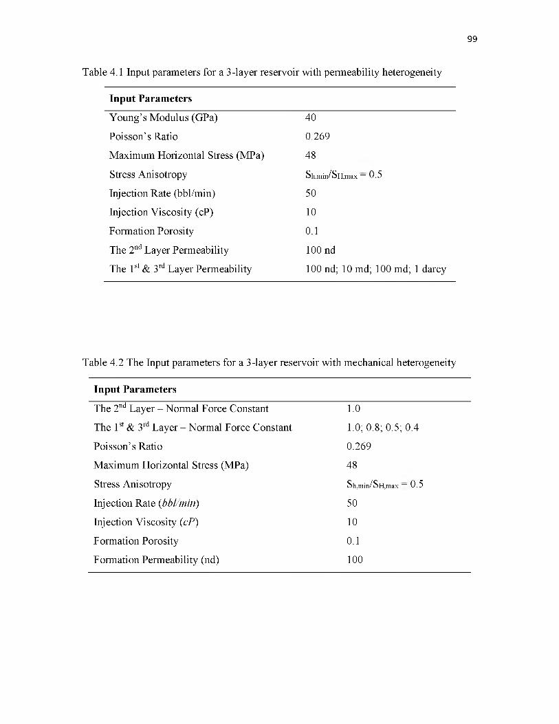
99

Table 4.1 Input parameters for a 3-layer reservoir with permeability heterogeneity

Input Parameters

Young’s Modulus (GPa) 40

Poisson’s Ratio 0.269

Maximum Horizontal Stress (MPa) 48

Stress Anisotropy Sh,min/SH,max _ 0.5

Injection Rate (bbl/min) 50

Injection Viscosity (cP) 10

Formation Porosity 0.1

The 2nd Layer Permeability 100 nd

The 1st & 3rd Layer Permeability 100 nd; 10 md; 100 md; 1 darcy

Table 4.2 The Input parameters for a 3-layer reservoir with mechanical heterogeneity

Input Parameters

The 2nd Layer - Normal Force Constant 1.0

The 1st & 3rd Layer - Normal Force Constant 1.0; 0.8; 0.5; 0.4

Poisson’s Ratio 0.269

Maximum Horizontal Stress (MPa) 48

Stress Anisotropy Sh,min/SH,max _ 0.5

Injection Rate (bbl/min) 50

Injection Viscosity (cP) 10

Formation Porosity 0.1

Formation Permeability (nd) 100

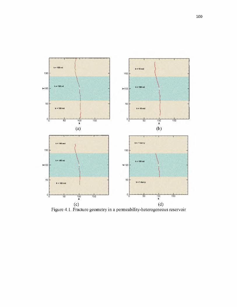
100

150

>100

, 1/

- (

k = 100 nd

i

. S _ \

\ -

\\

k = 100 nd ^

: t-

k = 100 nd

,0 50

50

100X

(a)

50 100X

150

I ' 1 1

k = 100 md

I '

(

- \\

-

k * 100 nd \

: ( -

k a 100 md

I . . . . . I .

150

>100 -

k = 1 darcy

>100 -

100 150X

(b)1—I--

100X

(c) (d)Figure 4.1. Fracture geometry in a permeability-heterogeneous reservoir

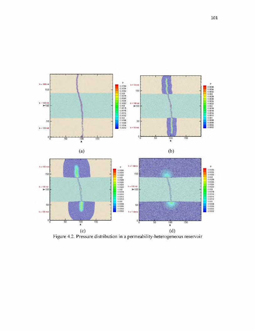
101

k = 100 nd

150

k = 100 nd >100

50

k = 100 nd

11 .

..............1____ .

I ;f;

i .

I

00036000340.00320.0030.0028000260.00240.00220.0020.00180.00160.00140.00120.0010.00080.00060.00040.0002

50 100X

150

(c) (d)Figure 4.2. Pressure distribution in a permeability-heterogeneous reservoir

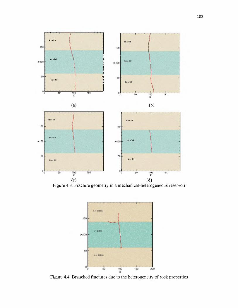
102

................................................. [ ....................................................................................kn = 1.0

kn s 1.0 \

........

........

........

........

..1....

........

........

........

....*..

........

........

........

.......

kn = 1.0

, ,

1 1

50 100 150

“ i 1------ '------r

150 -

0 50 150

150

> 1 0 0

150

50

50

(b)■ 1 •

kn = 0.4

■■ | ,

\

kn = 1.0

kn = 0.4

............................J . . . . ................................L........................ -100X

150

(c) (d)Figure 4.3. Fracture geometry in a mechanical-heterogeneous reservoir

Figure 4.4. Branched fractures due to the heterogeneity of rock properties

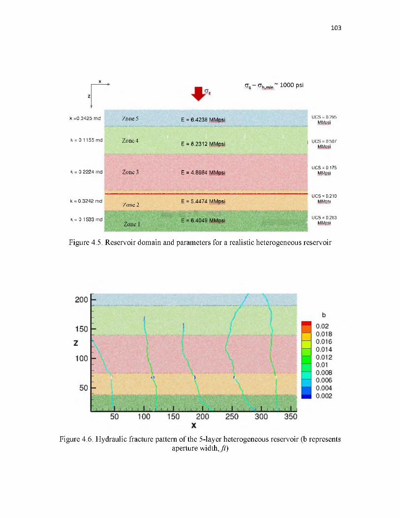
103

Sz Sh.mln 1000 psi

K =0 0425 md Zone 5 E = 6.4238 MMosi UCS = 0.295 MMpsi

k = 0.1155 md

k = 0.2224 md

k = 0 .3242 md

Zone 4

Zone 3

Zone 2

E = 8.2312 MMDsi

E = 4.8984 MMdsI

® il1 11 S§§fk = 0.1533 md

Zone 1

E = 5.4474 MMpsi

IE = 6.4049 MMpsi

I UCS = 0.507 MMpsi

- -

UCS = 0175 MMfisi

UCS = 0.210 MMpsi

UCS = 0.283 . w j j j j l l l i f M MMpsi

Figure 4.5. Reservoir domain and parameters for a realistic heterogeneous reservoir

Figure 4.6. Hydraulic fracture pattern of the 5-layer heterogeneous reservoir (b representsaperture width, ft)

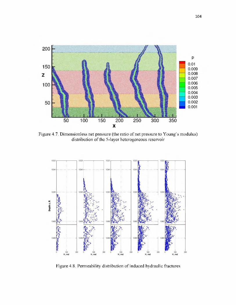
104

Figure 4.7. Dimensionless net pressure (the ratio of net pressure to Young’s modulus) distribution of the 5-layer heterogeneous reservoir

Figure 4.8. Permeability distribution of induced hydraulic fractures

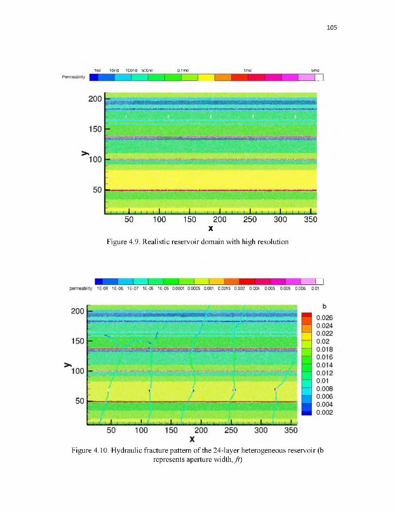
105

1 nd 10nd 100nd 500nd 0.1 md 1md 5md

l l l. , l , i ,l l , l M l l , l , l , , l l , j , l , l ■ , l 1 , 1 , 1 i l l l, , , 1 , , 1 „ 1 , l , , | „ l , i , | l , l

50 100 150 200 250 300 350X

Figure 4.9. Realistic reservoir domain with high resolution

Figure 4.10. Hydraulic fracture pattern of the 24-layer heterogeneous reservoir (brepresents aperture width, f t)

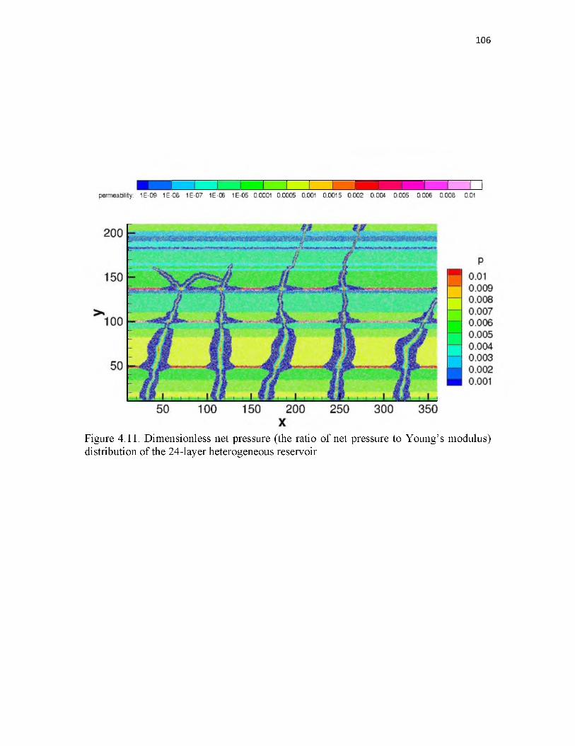
106

Figure 4.11. Dimensionless net pressure (the ratio of net pressure to Young’s modulus) distribution of the 24-layer heterogeneous reservoir

C H A PT E R 5

INTERACTION BETWEEN HYDRAULIC FRACTURES

AND NATURAL FRACTURES

In the previous chapters, a complex and fully coupled geomechanics and flow hydraulic

fracture propagation simulator based on Discrete Element Method has been proposed. Then

this simulator has been applied to both homogeneous and heterogeneous reservoirs with

single/multiple horizontal wellbores to predict the induced hydraulic fracture pattern. The

influences of completion strategies, including number of perforations, choice of injection

fluid, and wellbore, have also been investigated. However, in all those cases, the presence

of natural fractures has not been considered.

5.1 Introduction

It has been widely observed from experiments and microseismic observations that

hydraulically induced fractures in a shale reservoir often deviate from the conventional bi­

wing fracture geometry and lead to the formation of a complex fracture network, which

may be caused by the stress shadow effect from multiple hydraulic fractures or interaction

with pre-existing natural fractures. According to well-log data, in reservoirs with ultra-low

permeability, such as Barnett, the natural fractures are widely distributed, which will result

in hydraulic fractures branching and merging at the Hydraulic Fracture (HF)-Natural

Fracture (NF) interface and consequently lead to the creation of the complex fracture

network. The opening of natural fractures will provide additional flow paths for

hydrocarbons, with the potential of enhancing the recovery factor. Therefore,

understanding the interaction between HF and NF plays a crucial role in quantifying the

stimulated reservoir volume (SRV) and optimizing the well completion strategy in

unconventional reservoirs.

As shown in Figure 5.1, several possibilities exist when the hydraulic fracture intersects

with natural fractures:

(1) The hydraulic fracture directly crosses the natural fracture and keeps propagating

in its original direction. Under such conditions, the fracture will remain planar.

(2) The hydraulic fracture crosses the natural fracture with an offset, where the

hydraulic fracture will deflect into the natural fracture for a certain distance and

resume its propagation into the formation along the maximum stress direction at

some weak points in the natural fracture. A small portion of the natural fracture will

be reactivated to become a part of a generated effective fracture network.

(3) The hydraulic fracture will be arrested at the HF-NF intersecting point, proceed

along the path of the natural fracture to its tip and then propagate into the formation.

If the natural fracture is not perpendicular to the hydraulic fracture, the natural

fracture will be opened only in one direction.

(4) The hydraulic fracture branches at the intercepting point, partly diverting into the

natural fracture and partly crossing the natural fracture.

Under certain circumstances, the natural fractures will be reactivated or dilated by the

hydraulic fractures and thus lead to the formation of a complex fracture pattern. The

108

different scenarios that may play out in the HF-NF interactions depend on many

parameters, including in-situ stress, rock formation properties, natural fracture properties

and orientation, and injection fluid viscosity and rate. A number of methods have been used

and tried to understand the combined effects of these parameters on the morphology of the

generated fracture network [92].

Extensive experimental research has been conducted to investigate the HF-NF

interaction and the effects of different parameters. Warpinski [93], Teufel [94] and Blanton

[95] used hydrostone and sandstone to examine the effects of interface angles and stress

conditions on the induced facture pattern, which revealed that the hydraulic fracture tends

to arrest and divert into the natural fracture under small stress difference and small joint

orientation. Based on the laboratory results, some criteria have been developed to explain

the HF-NF intercepting behavior and provide a basis for projecting the experimental results

to field cases.

Considering the high expense of getting a core sample representative of the

heterogeneities in unconventional reservoirs, microseismic data provide an alternative way

to predict and map the induced fracture network in naturally fractured reservoirs. Fisher

[96] indicated that multiorientated hydraulic fractures are generated due to the pre-existing

natural fractures by analyzing the Barnett microseismic data. Generally, a microseismic

event is a widespread cloud surrounding the hydraulic fracture that is caused by shear

failure along the weak plane [31], from which the stimulated reservoir volume will be

obtained. However the resolution of this data is too coarse to describe the exact hydraulic

fracture planes. Moreover, both the experimental and microseismic data cannot predict the

detailed growth and interacting behaviors of hydraulic fractures in large-scale reservoirs.

109

Numerical modeling provides another powerful avenue to examine the reactivation of

natural fractures. A robust numerical model should be able to capture:

1. Hydraulic fracture propagation and the stress shadow effect.

2. Fluid flow in both the formation and multiple fractures.

3. Multiple interaction mechanisms between hydraulic fracture and natural fracture.

Research on modeling nonplanar hydraulic fracture growth has progressed

significantly in recent years. Criteria for the interaction and subsequent development of

complex fracture networks have been examined. Renshaw and Pollard [97] and Gu and

Weng [98] proposed criteria to predict fracture propagation across a frictional interface

with different intersection angles based on linear elastic fracture mechanics. Chuprakov et

al. [99] developed an analytical crossing model by combining the effect of mechanical

interaction and fluid properties. Dahi-Taleghani and Olson [100] proposed a new criterion

dealing with the interception of the hydraulic fracture with a fully cemented natural fracture

based on energy-release rate.

The displacement discontinuity method (DDM) is one of the most popular methods

utilized in hydraulic fracture propagation modeling for its high efficiency and accuracy.

Sesetty and Ghassemi [101] developed a hydraulic fracture propagation simulator based

on DDM. In order to improve the accuracy, the model uses square-root tip elements to

calculate the stress intensity factor. A maximum stress criterion is used to predict the angle

at which the fracture will grow after intersecting with natural fracture. Kresse et al. [102]

proposed a semianalytical unconventional fracture model (UFM, OpenT) that includes

both the fracture interaction and flow rate effect in the simulation. Also based on the DDM

concept, the OpenT simulator can capture the influences of fracture orientation, natural

110

fracture friction coefficient, and in-situ stress on HF-NF interactions. Wu and Olson [103]

developed a simplified three-dimensional DDM model to simulate the HF-NF interaction

and investigated the effect of natural fracture length, in-situ stress, and relative angle on

the induced fracture pattern. Two different crossing criteria are used to predict the

interaction behavior at the frictional interface and with fully cemented natural fractures.

Huang et al. [104], [105] combined geomechanics simulation based on DDM with

microseismic data to calibrate the numerical model and applied it to Barnett shale

formation. Those DDM-based models can simulate the complex interaction between

hydraulic fracture and natural fracture, but with the strict assumption of the formation being

homogeneous.

Dahi-Taleghani and Olson used an Extended Finite Element Method (XFEM) model

to simulate the hydraulic fracture interaction with natural fractures. The XFEM can handle

heterogeneous reservoirs and complex boundary conditions, but at the expense of a heavy

computational load.

In this chapter, the method proposed in Chapter 2 will be used to simulate the HF/NF

interactions. Since the fracture initiation is simulated by the breaking of particle bonds and

the aperture is obtained through the displacement of rock particles, no additional fracture-

crossing criterion is required in determining HF/NF intersecting behavior. The

implementation of a natural fracture in our DEM simulator is proposed in Section 5.2. Then

a simple case of hydraulic fracture and natural fracture interaction is used to illustrate the

capability of our simulator. Finally, the effects of hydraulic fracture approach angle, in-situ

stress anisotropy, and natural fracture properties including permeability and cohesion,

injection rate, and viscosity on HF-NF interaction will be investigated.

111

5.2 Representation of Natural Fractures

As discussed in Chapter 2, the rock is mimicked by an assembly of small particles with

beam connections. The hydraulic fracture’s propagation length and direction are simulated

by the bond breakage. As shown in Figure 5.2, the pre-existing natural fractures in my

research are realized by breaking or weakening the bonds between DEM particles along

the natural fractures. Based on the knowledge of natural fracture locations which can be

obtained from Formation Microseismic Imaging (FMI) of logs or core data, a series of

DEM bonds are created and linked to explicitly represent the natural fractures. The natural

fractures can be fully opened or cemented depending on the type and extent of filling in

these fractures. This is done by applying a cohesion coefficient to define the weakness of

natural fractures.

Since the DEM particles are distributed randomly, the natural fractures represented in

this way are not perfectly straight and have inherent frictional forces. There are two ways

to reduce the frictional force:

1. Reduce the size of particles, which results in a more regular particle distribution.

2. Insert a frictionless plane before generating the DEM particles.

The predefined discontinuities/weak planes can have different properties by changing

the location, orientation, strength and permeability. Therefore, in this model, the natural

fractures may also be treated as a small heterogeneous zone. Whether the natural fracture

will be reactivated or remain closed is directly reflected by the DEM particle displacement,

and no empirical formula or analytical crossing criterion is required.

112

5.3 Simple Case of HF and NF Interaction

In this section, the interaction of single hydraulic fracture with single natural fractures

will be examined to illustrate the evolution of the HF-NF interaction process and the

capability of our developed simulator. Figure 5.3 shows the schematic reservoir model used

in this paper. The reservoir is homogeneous and isotropic, with a size of 200 f t x 200 ft.

The radius of all circular DEM particles lies between 0.4 f t to 0.6 ft, thus nearly 51000

particles are generated in total. A horizontal well with single perforation is located at the

bottom of the domain aligned along the minimum stress direction, and only one main

hydraulic fracture will be generated through injection process. In this two-dimensional

model, we assume the induced fracture to have a constant height in z direction. The

maximum horizontal stress is oriented in the _y-direction. The detailed reservoir parameters

and rock properties are provided in Table 5.1.

As shown in Figure 5.3, the natural fracture is located at the center of the reservoir

domain with the orientation perpendicular to the maximum horizontal stress. Due to the

random packing of DEM particles and the way of defining natural fracture in our simulator,

the natural fracture will not be perfectly straight. The permeability of NF is 1 md, injection

viscosity is 10 cP and the in-situ stress is large (Shmtn/Snmax = 0.5). The natural fracture is

assumed to be in equilibrium under the initial far-field stress condition. Figure 5.4 shows

how the induced hydraulic fracture interacts with the natural fracture.

The pressure in the wellbore builds up on injection of the fracturing fluid. Once the

pressure at the perforation is large enough to break a DEM particle bond, a microcrack will

initialize, coalesce, and propagate further. Since the whole system is assumed to be at

equilibrium initially, the presence of the natural fracture will not significantly impact the

113

hydraulic fracture growth until the hydraulic fracture reaches the natural fracture.

Therefore, without stress interference from other induced fractures, the hydraulic fracture

will propagate in the preferential direction that is parallel to the far-field maximum stress

direction, as shown in Figure 5.4 (a).

An interesting phenomenon is observed in Figure 5.4 (b). When the hydraulic fracture

approaches the natural fracture (before intersection), some spots on the natural fracture

begin to exhibit opening/aperture. One reason for this is that when hydraulic fracture and

natural fracture get closer, the stress concentration around the hydraulic fracture tip will

change the stress condition around the natural fracture, causing the movement of some

DEM particles. Taking into consideration that the particles representing natural fracture

have no bond connections (cohesion equals zero), natural fracture may experience sliding

before contact with hydraulic fracture.

With continued fluid injection, the hydraulic fracture grows and intercepts the natural

fracture (Figure 5.4 (c)). Since the natural fracture’s cohesion is set to zero, the natural

fracture interface is much weaker than the rock formation. In addition, the permeability of

natural fracture (1 md) is much greater than the formation permeability (100 nd). Therefore,

some injected fluid will penetrate into the natural fracture. Due to these two factors, natural

fracture will open, leading to the arresting of the growth of hydraulic fracture. However,

due to the large initial stress contrast, the pressure required to fully reactivate the natural

fracture is high. The natural fracture is not opened along its entire length, and the hydraulic

fracture will reinitiate at some weak point along the natural fracture and keep propagating

close to the original direction with a small offset (Figure 5.4 (d)). Once the hydraulic

fracture departs from the natural fracture, the compressive stress exerted may close the

114

115

previously opened natural fracture. Complex interactions between these attributes of the

natural fracture and hydraulic fracture are fully captured by the model.

The net injection pressure at the injection point is shown in Figure 5.5. In this figure,

the red, green, and purple dotted lines, respectively, represent the times when hydraulic

fracture starts to propagate (Point A), the hydraulic fracture intersect with natural fracture

(Point B), and the generated fracture reaches to reservoir boundary (Point C). It is obvious

that pressure keeps building up until hydraulic fracture intercepts with the natural fracture

(Point B). After that, the pressure at the wellbore begins to drop due to the fluid leakoff

into the natural fracture. However, since the natural fracture cannot be fully reactivated by

injection and the hydraulic fracture goes back to propagate into the formation, the pressure

will not experience a significant drop. In addition, because of the low permeability of the

formation and the relatively small domain, the hydraulic fracture will reach the boundary

very quickly after leaving the natural fracture. Once the induced fracture reaches the

boundary, the pressure at the wellbore will start building up again because of the no-flow

boundary condition.

5.4 Sensitivity Analysis

In this section, sensitivity analyses will be conducted to investigate different parameters

which affect HF-NF interactions. All parameters can be categorized into:

1. Geological parameters, including natural fracture orientation, cohesion,

permeability, and stress anisotropy.

2. Controllable operational parameters, such as injection rate and viscosity.

5.4.1 Effect of Natural Fracture Orientation

Microseismic data suggest that natural fractures commonly exist in most

unconventional reservoirs, especially in shale formations. Natural fractures may be present

with multiple orientations within the reservoir, and may not be fully aligned with the

current principal in-situ stress direction. For example, a number of natural fractures appear

to be parallel to the minimum horizontal stress in Barnett shale [106]. Four different

intersection angles a (angle between natural fracture and maximum horizontal stress) are

used: 90o, 75o, 45o, and 30o. The stress anisotropy ratio is 0.7 (Sh,min/SH,max = 0.7) for all

cases, the natural fracture permeability is 1 md, and the injection fluid viscosity is 10 cP.

The induced fracture behaviors are shown in Figure 5.6.

From Figure 5.6, it is obvious that the orientation of NF will significantly affect the

induced fracture’s development. If the intersection angle is large (>= 75o), the hydraulic

fracture tends to directly cross the natural fracture without opening it. The hydraulic

fracture will divert into the natural fracture and is arrested at the contacting point, if the

angle is decreased. The injection fluid flows along the natural fracture and reactivates it.

Therefore, the dilated natural fracture becomes part of an effective hydraulic fracture

network. The hydraulic fracture will continue growing along the natural fracture

orientation. The possible reasons which lead to the propagation along the natural fracture

direction rather than in-situ maximum stress direction after reaching the tip of NF are:

1. The stress difference being not sufficiently large.

2. The opening of the natural fracture will alter the local principal stress direction.

3. The natural fracture orientation is already close to the maximum horizontal stress

direction.

116

Moreover, once the hydraulic fracture deflects into the natural fracture with a

nonorthogonal angle, it will reactivate the natural fracture only in one direction, which is

the part formed of an oblique-angle intersection with the hydraulic facture. The direction

with an obtuse angle is more close to the original fluid flow path and far field maximum

stress direction that is less resistant to opening. This propagating direction preference from

numerical simulation also matches the theoretical analysis [36], [63].

Therefore, the results indicate that for nonorthogonal interaction, the intercepting angle

will greatly affect the generated fracture morphology. With a large intercepting angle, the

hydraulic fracture tends to cross the NF and remain bi-wing planar in geometry; on the

contrary, a small intercepting angle is more favorable for opening the natural fracture and

generating a complex network.

5.4.2 Effect of Natural Fracture Cohesion

The previous example assumes that the natural fracture has zero cohesion, which is

implemented by breaking all natural fracture bonds in the simulation. However, core

observations indicate that natural fractures in many shale formations are largely sealed with

minerals [106]. Therefore, natural fractures may not necessarily be fully open or may not

be totally cemented in reality. In this section, we are going to investigate the affect of

natural fracture cohesion on fracture generation.

The bonds representing the natural fracture are weakened at different levels, which are

described through the cohesion coefficient (natural fracture strength = cohesion coefficient

x formation rock strength). The smaller the cohesion coefficient, the weaker the bond. Four

different cohesion coefficients are used here: 0, 0.3, 0.6, and 0.9, and all other properties

117

are kept the same: the residual permeability of natural fracture is 1 md, in-situ stress

anisotropy ratio is 0.7 (Sh,mtr/Sn,mcx = 0.7), the intersection angles a (angle between natural

fracture and maximum horizontal stress) is 45o, and the injection viscosity is 10 cP. The

maximum stress direction is still oriented in the y-direction. The induced fracture patterns

are summarized in Figure 5.7.

As cohesion increases, the strength of the natural fracture is getting closer to the rock

formation strength. The value of the cohesion coefficient assigned to the fracture

determines whether the intercepting HF is going to reactivate the NF or cross the fracture.

The transition to partial reactivation occurs at a cohesion coefficient value of 0.3, while for

values larger than 0.9, the NF is not even partially reactivated.

5.4.3 Effect of Natural Fracture Permeability

Beside the natural fracture orientation and cohesion, the permeability of NF will also

affect HF geometry. The effect of natural fracture permeability is examined by comparing

the following two cases with different NF permeability: one is 1 m d and the other one is

10 Darcy. In both cases, NF has much greater permeability compared with formation

permeability (100 nd). In order to remove other possible disturbances to fracture geometry,

we use the same injection fluid (10 cP and 0.01 m2/s), in-situ stress anisotropy (Sh,mtn/Sn,max

= 0.7), cohesion (0), and the same natural fracture orientation (90o). Other formation

parameters are the same as in previous examples. The profiles of generated fractures are

shown in Figure 5.8.

The hydraulic fracture crosses the natural fracture directly when the natural fracture

permeability is small. Even though the natural fracture is a weak plane with zero cohesion,

118

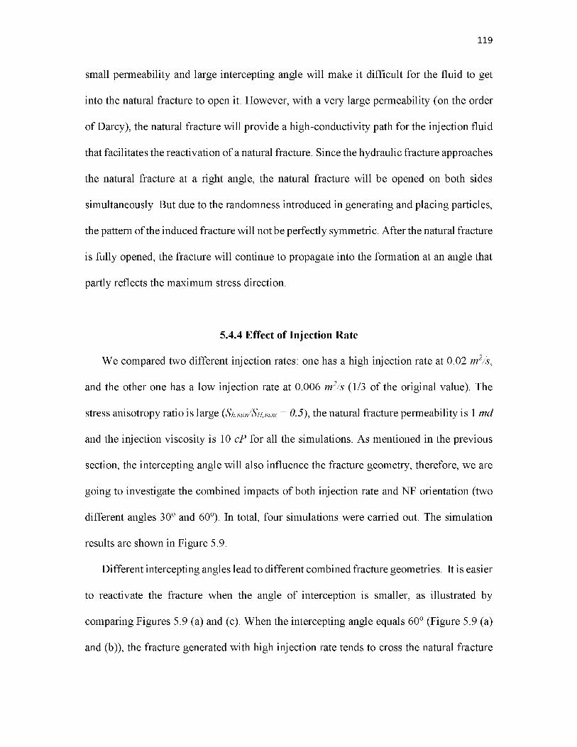
119

small permeability and large intercepting angle will make it difficult for the fluid to get

into the natural fracture to open it. However, with a very large permeability (on the order

of Darcy), the natural fracture will provide a high-conductivity path for the injection fluid

that facilitates the reactivation of a natural fracture. Since the hydraulic fracture approaches

the natural fracture at a right angle, the natural fracture will be opened on both sides

simultaneously. But due to the randomness introduced in generating and placing particles,

the pattern of the induced fracture will not be perfectly symmetric. After the natural fracture

is fully opened, the fracture will continue to propagate into the formation at an angle that

partly reflects the maximum stress direction.

5.4.4 Effect of Injection Rate

We compared two different injection rates: one has a high injection rate at 0.02 m2/s,

and the other one has a low injection rate at 0.006 m2/s (1/3 of the original value). The

stress anisotropy ratio is large (Sh,min/SH,max = 0.5), the natural fracture permeability is 1 md

and the injection viscosity is 10 cP for all the simulations. As mentioned in the previous

section, the intercepting angle will also influence the fracture geometry, therefore, we are

going to investigate the combined impacts of both injection rate and NF orientation (two

different angles 30o and 60o). In total, four simulations were carried out. The simulation

results are shown in Figure 5.9.

Different intercepting angles lead to different combined fracture geometries. It is easier

to reactivate the fracture when the angle of interception is smaller, as illustrated by

comparing Figures 5.9 (a) and (c). When the intercepting angle equals 60o (Figure 5.9 (a)

and (b)), the fracture generated with high injection rate tends to cross the natural fracture

directly and proceed at the orientation parallel to the far-field maximum stress direction.

With the smaller injection rate, the hydraulic fracture will divert into the natural fracture

and dilate the NF. This observation is confirmed by experiments [102]. Once the injection

fluid gets accepted by the natural fracture, the net pressure in the NF will increase and drive

the opening of NF. At the tip of NF, the fracture will curve back to the far-field stress

direction due to the large stress anisotropy.

We observe that the fracture branching effect occurs at the HF-NF interface with the

high injection rate by reducing the intercepting angle to 30o, which is more favorable for

the dilating of natural fracture. Based on the fracture propagation process, the natural

fracture is opened by the injected fluid first, then the “branching” fracture is generated at

the contacting point. This branching phenomenon is caused by the competition between

dilating-favorable NF angle and crossing-favorable injection rate. In addition, the

branching fracture is found to propagate along the direction deviated from the far-field

maximum stress. The reason is that the opening of the natural fracture will exert additional

compressive stress in the neighborhood and reorient the local principal stress direction,

which will drive the branching fracture away from the reactivated natural fracture.

Moreover, by comparing Figure 5.9 (b) and (d), for large intercepting angle, the fracture

will more easily turn back toward the original orientation of the hydraulic fracture.

5.4.5 Effect of Injection Viscosity

In industry, the fluid used for hydraulic fracturing varies from low-viscosity slick water

to high-viscosity gel. A scenario with multiple natural fractures is considered. Two

simulations with different fluid viscosity are used here: 10 cP and 800 cP. Fifty-three

120

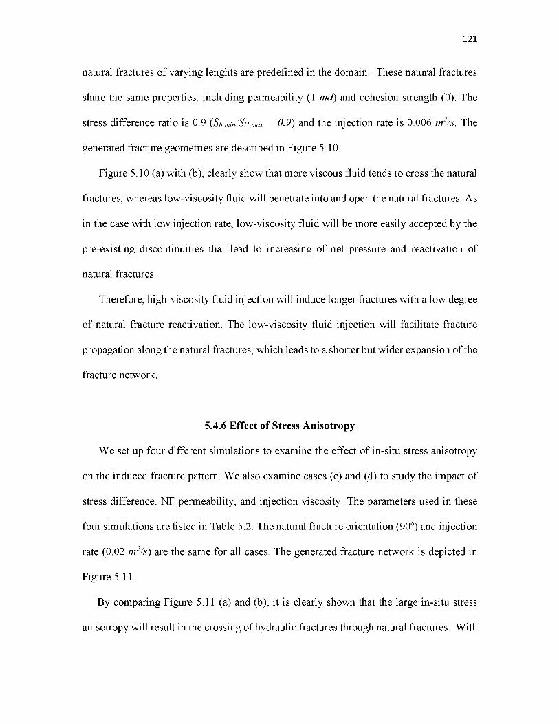
natural fractures of varying lenghts are predefined in the domain. These natural fractures

share the same properties, including permeability (1 md) and cohesion strength (0). The

stress difference ratio is 0.9 (Sh,min/SH,max = 0.9) and the injection rate is 0.006 m2/s. The

generated fracture geometries are described in Figure 5.10.

Figure 5.10 (a) with (b), clearly show that more viscous fluid tends to cross the natural

fractures, whereas low-viscosity fluid will penetrate into and open the natural fractures. As

in the case with low injection rate, low-viscosity fluid will be more easily accepted by the

pre-existing discontinuities that lead to increasing of net pressure and reactivation of

natural fractures.

Therefore, high-viscosity fluid injection will induce longer fractures with a low degree

of natural fracture reactivation. The low-viscosity fluid injection will facilitate fracture

propagation along the natural fractures, which leads to a shorter but wider expansion of the

fracture network.

5.4.6 Effect of Stress Anisotropy

We set up four different simulations to examine the effect of in-situ stress anisotropy

on the induced fracture pattern. We also examine cases (c) and (d) to study the impact of

stress difference, NF permeability, and injection viscosity. The parameters used in these

four simulations are listed in Table 5.2. The natural fracture orientation (90o) and injection

rate (0.02 m2/s) are the same for all cases. The generated fracture network is depicted in

Figure 5.11.

By comparing Figure 5.11 (a) and (b), it is clearly shown that the large in-situ stress

anisotropy will result in the crossing of hydraulic fractures through natural fractures. With

121

large differential stress, the natural fracture requires higher injection pressure to open. The

resistance for entry into the natural fracture will be higher. The fact that it is more difficult

to reactivate the natural fracture when the stress anisotropy is smaller is consistent with

experimental observations and other numerical simulations [107]. Figure 5.11 (b) shows

that instead of being fully diverted into the natural fracture, the fracture has been separated

into two strands, both opening and crossing the natural fracture when the stress difference

is small. The small differential stress will make the natural fracture much easier to open,

however the unfavorable orientation and small permeability of the natural fracture will

impede the fluid flow into the natural fracture. With relatively high injection rate, the

hydraulic fracture crosses over. The branching effect will disappear if the injection rate

becomes lower or the natural fracture permeability is much higher (referred to Figure 5.9

(b)).

Figure 5.11 (c) and (d) provide another example of in-situ stress effect when the natural

fracture permeability is relatively high (on the order of Darcy). From Figure 5.11 (c), it is

observed that rather than directly crossing the natural fracture and remaining planar, the

hydraulic fracture exhibits a double-branching phenomenon at the HF-NF interface under

high-stress anisotropy. This can be attributed to the high permeability and zero cohesion of

the natural fracture. Due to the weakness of the natural fracture and the high permeability,

the fluid leaks off into the natural fracture at the beginning of interaction. It goes in both

directions due to the intersecting angle being 900. There is infusion of a small amount of

fluid in both the branches in the multistrand propagation. The large stress anisotropy will

force the branched fractures to cross the natural fracture and propagate along the maximum

horizontal stress direction. In addition, the opening of fractures will induce additional

122

compressive stresses and alter the local principal stress direction that will make the two

branching fractures repel each other. The fracture pattern for low anisotropy is shown in

Figure 5.11 (d). With a small stress difference, the natural fracture is much easier to open

and dilate. However, the large intercepting angle and high viscosity will inhibit the opening

of the fracture on both sides. Therefore, a branching fracture grows from the point of

contact.

5.5 Summary

The novel dual-lattice, fully coupled hydro-mechanical hydraulic fracture simulator

presented in the Chapter 2 is able to simulate the propagation of hydraulic fractures in

naturally fractured reservoirs. The computations are able to capture a variety of HF-NF

interactions, such as crossing, dilating, and branching. The effects of in-situ stress, natural

fracture properties (orientation, cohesion, and permeability), and injection fluid properties

(injection rate and viscosity) are also examined in this chapter.

• In-situ stress anisotropy has significant effect on the induced fracture geometry. The

larger the stress difference, the harder it is to reactivate natural fractures. The

hydraulic fracture remains planar after intercepting and crossing the natural fracture.

• Larger intercepting angle, larger natural fracture cohesion coefficient, or smaller

natural fracture permeability make it more difficult for fluid intrusion and

reactivation of the natural fracture and facilitate the uninhibited growth of the

hydraulic fractures.

• Lower injection rates or lower injected fluid viscosities lead to a higher amount of

fluid intake into the natural fractures, leading to their reactivation.

123

124

• The hydraulic fracture will branch off if the factors favoring natural fracture fluid

leakoff and reactivation are comparable with those favoring continued growth.

The results presented in this chapter provide guidelines for controlling hydraulic

fracture morphology in naturally fractured reservoirs. If a more connected network is

desired, it is better to use lower injection rates and fluids with lower viscosities.

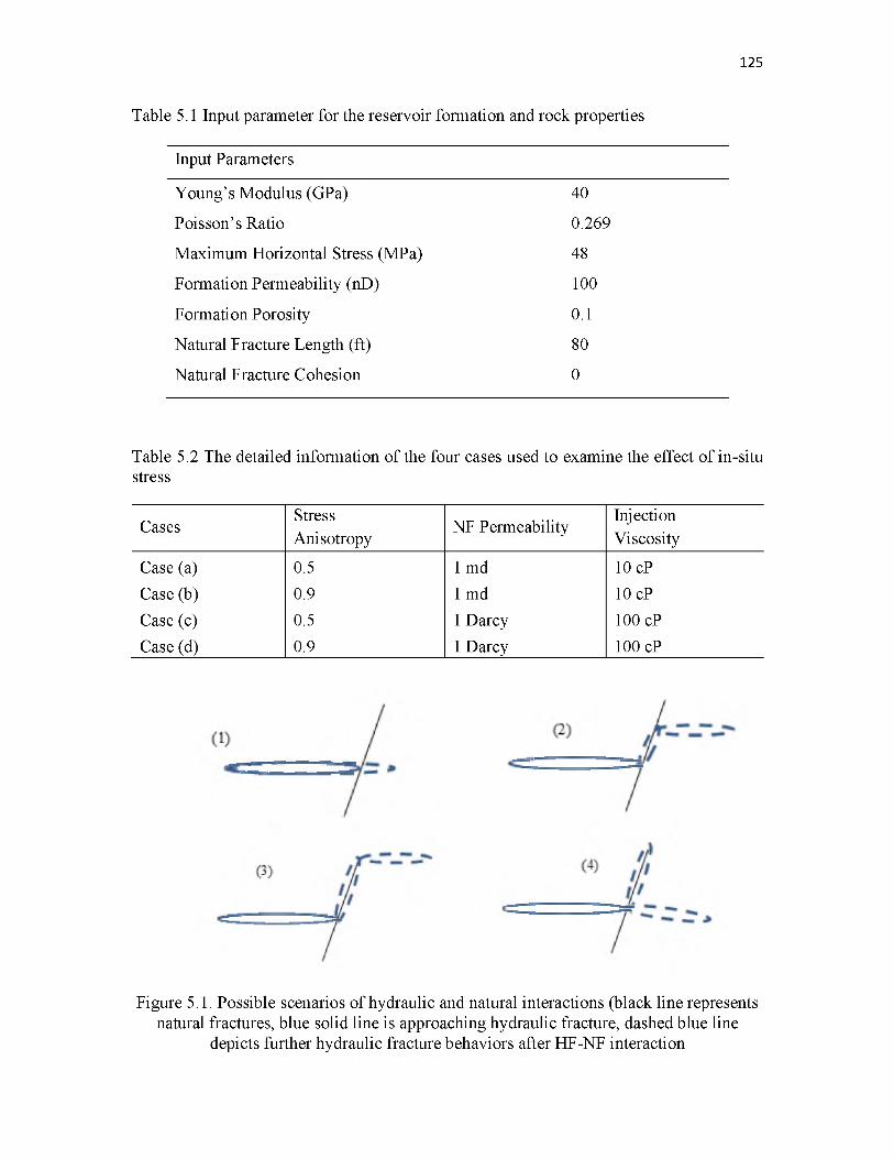
125

Table 5.1 Input parameter for the reservoir formation and rock properties

Input Parameters

Young’s Modulus (GPa) 40

Poisson’s Ratio 0.269

Maximum Horizontal Stress (MPa) 48

Formation Permeability (nD) 100

Formation Porosity 0.1

Natural Fracture Length (ft) 80

Natural Fracture Cohesion 0

Table 5.2 The detailed information of the four cases used to examine the effect of in-situ stress

CasesStressAnisotropy

NF PermeabilityInjectionViscosity

Case (a) 0.5 1 md 10 cP

Case (b) 0.9 1 md 10 cP

Case (c) 0.5 1 Darcy 100 cP

Case (d) 0.9 1 Darcy 100 cP

Figure 5.1. Possible scenarios of hydraulic and natural interactions (black line represents natural fractures, blue solid line is approaching hydraulic fracture, dashed blue line

depicts further hydraulic fracture behaviors after HF-NF interaction

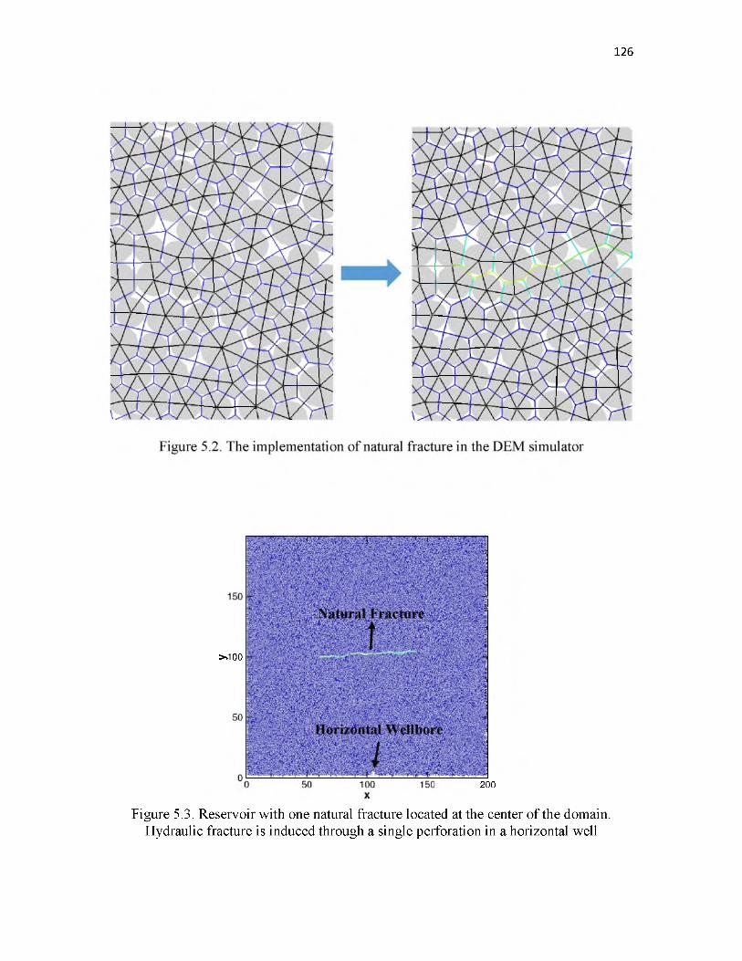
126

>.100

200

Figure 5.3. Reservoir with one natural fracture located at the center of the domain. Hydraulic fracture is induced through a single perforation in a horizontal well

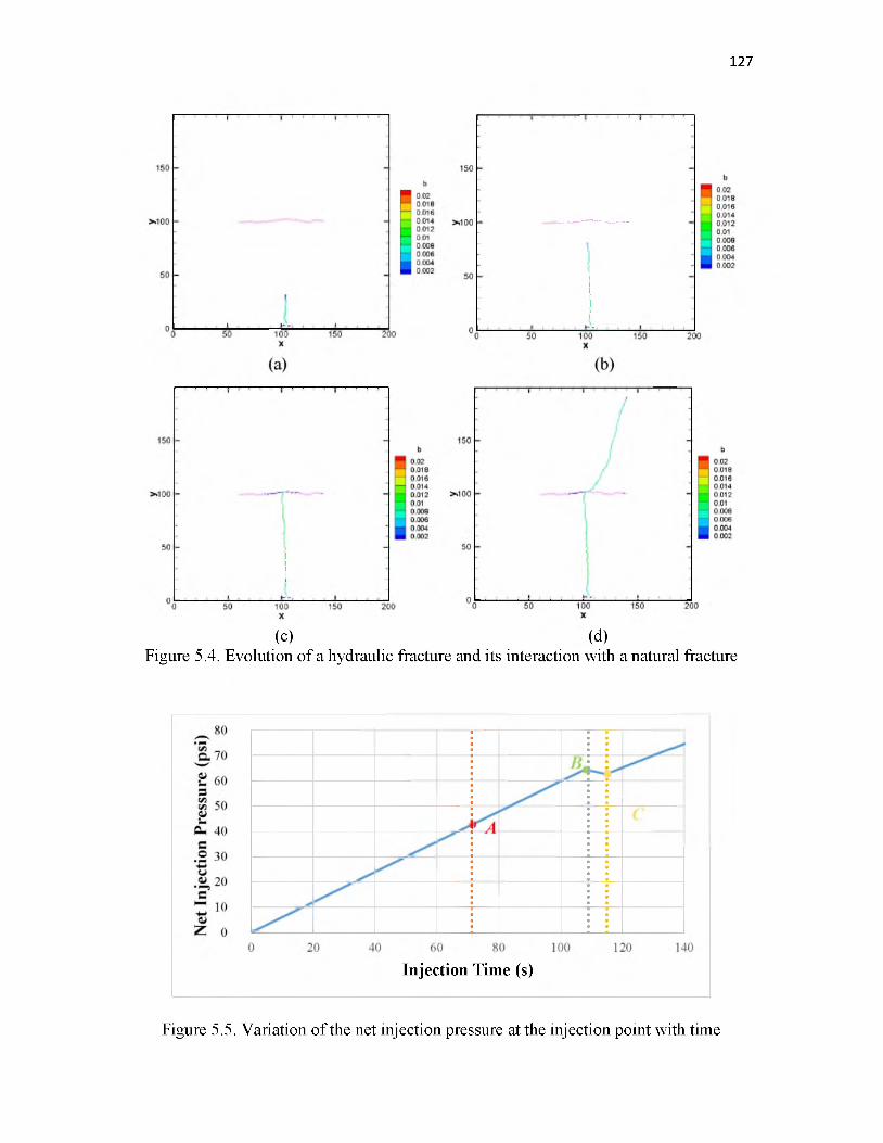
127

(c) (d)Figure 5.4. Evolution o f a hydraulic fracture and its interaction with a natural fracture

Injection Time (s)

Figure 5.5. Variation o f the net injection pressure at the injection point with time

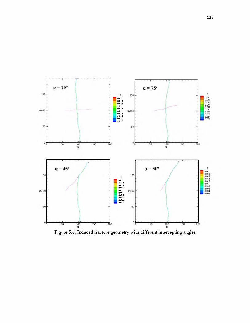
128

0.020.0180.0160.0140.0120.010.0080.0060.0040.002

0.020.0180.0160.0140.0120.010.0080.0060.0040.002

0.020.0180.0160.0140.0120.010.0080.0060.0040,002

Figure 5.6. Induced fracture geometry with different intercepting angles

129

0.02

0.0180.0160.0140.0120.010.0080.0060.0040.002

I I 1 I I 1 I I 1.......................................

- C ohes ion = 0 .9

' ‘

j '

I— ......................................100X

Figure 5.7. Induced fracture geometry with different natural fracture cohesion

0.020.0180.0160.0140.0120.010 0080.0060.0040.002

150

>100

Figure 5.8. Induced fracture geometry with different natural fracture permeability

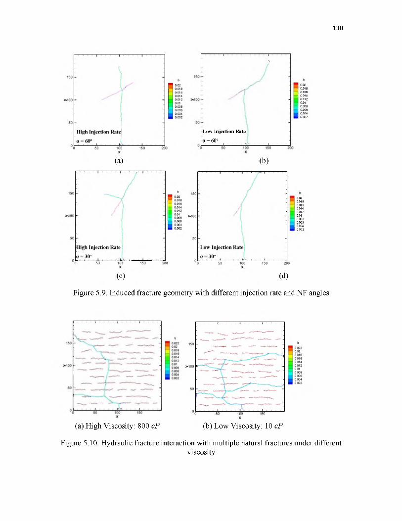
130

(a)

1 1 1. »

Low Injection Rate

a = 60o. i : i

(b)

0.02 0.018

1 0.016 I 0.014

0.012 0.01

| 0.008 j 0.006

0 004I 0.002

0.020.0180.0160.0140.0120.010.0080.0060.004

I 0.002

(c) (d)

Figure 5.9. Induced fracture geometry with different injection rate and NF angles

(a) High Viscosity: 800 cP (b) Low Viscosity: 10 cP

Figure 5.10. Hydraulic fracture interaction with multiple natural fractures under differentviscosity

131

0.020.0180.0160.0140.0120.010.0080.0060.0040.002

(a) (b)

0,020.0180.0160.0140.0120.010.0080.0060.0040.002

0.020.0180.0160.0140.0120.010.0080.0060.0040.002

(c) (d)

Figure 5.11. Induced fracture geometry with different stress condition (legend shows thefracture width)

C H A PT E R 6

COMBINATION OF REALISTIC FRACTURE GEOMETRY

WITH FLOW SIMULATOR

Forty-nine percent of total oil production in the USA and 54% of gas production in

February 2015 came from fractured reservoirs (EIA data). Multiple vertical fractures in a

horizontal well create large a stimulated reservoir volume (SRV). High flow areas in SRV

make it possible to produce from ultralow-permeability reservoirs. In order to predict

recovery from the unconventional reservoir through numerical simulation, the common

practice in industry is to assume a planar orthogonal fracture, which may be incorrect and

misleading. In this section, we are going to predict hydrocarbon recovery with more

realistic nonplanar fracture geometry obtained from a DEM simulation and compare it with

orthogonal fractures. In Section 6.1, the nonplanar fractures will be mapped into a regular

Cartesian grid mesh. The mapped reservoir domain with hydraulic fractures will be inserted

into the flow simulator to predict the production in Section 6.2.

6.1 Mapping of the Hydraulic Fracture

Figure 6.1 shows the two different fracture geometries used in this section. Figure

6.1(a) is the most widely used fracture geometry in the flow simulator - a planar and

orthogonal fracture with single property such as length, width and permeability. Figure

6.1 (b) is the fracture geometry generated through the DEM simulator proposed in the

thesis. As shown in the previous section, the generated fractures are nonplanar, with

varying apertures. In order to compare the effect of fracture geometry on recovery factor,

the first thing is to map these nonplanar fractures into a regular mesh that is applicable to

flow simulator.

Currently, it is still very challenging to precisely model a nonplanar fracture using

numerical flow simulator. In this section, we are using the zigzag fracture pattern to

approximate nonplanar fracture geometry [108].

The mesh size of the domain used in the flow simulator is fixed. In the zigzag mapping,

we assume that the nonplanar fracture is composed of many connected line segments of a

specific length. The principle of this mapping technology is to ensure that the

conductivities of the fractures in the DEM model and the flow simulator are matched.

kf,DEMbf,DEM = kfjiow bfjlow (61)

where kf DEM and b ,̂DEM are the fracture permeability and aperture obtained from the

DEM simulator. kf j iow and bf j i ow are the fracture permeability and aperture used in the

flow simulator. Figure 6.2 shows an example of nonplanar fractures generated through the

DEM simulator which has been separated into 12 small zones. We use zone 2 as an example

to illustrate the zigzag mapping technology.

Figure 6.3 (a) shows that the fracture is represented through a series of connected lines.

Since the fracture initiation in the DEM simulator is mimicked by DEM particle bond

breakage, the length and direction of the small line are determined by the DEM particles’

location used to connect by the broken bond. Each line segment owns different property.

Then those nonuniform properties will project into the mesh grid used in the flow simulator

133

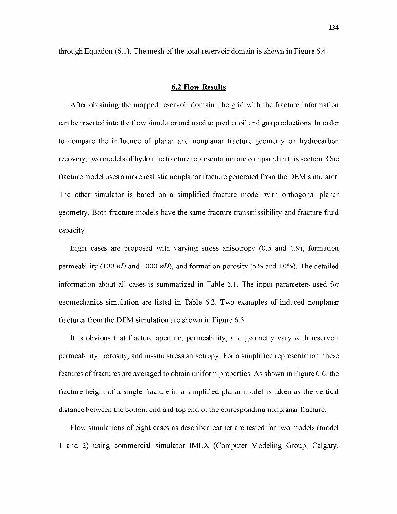
134

through Equation (6.1). The mesh of the total reservoir domain is shown in Figure 6.4.

6.2 Flow Results

After obtaining the mapped reservoir domain, the grid with the fracture information

can be inserted into the flow simulator and used to predict oil and gas productions. In order

to compare the influence of planar and nonplanar fracture geometry on hydrocarbon

recovery, two models of hydraulic fracture representation are compared in this section. One

fracture model uses a more realistic nonplanar fracture generated from the DEM simulator.

The other simulator is based on a simplified fracture model with orthogonal planar

geometry. Both fracture models have the same fracture transmissibility and fracture fluid

capacity.

Eight cases are proposed with varying stress anisotropy (0.5 and 0.9), formation

permeability (100 nD and 1000 nD), and formation porosity (5% and 10%). The detailed

information about all cases is summarized in Table 6.1. The input parameters used for

geomechanics simulation are listed in Table 6.2. Two examples of induced nonplanar

fractures from the DEM simulation are shown in Figure 6.5.

It is obvious that fracture aperture, permeability, and geometry vary with reservoir

permeability, porosity, and in-situ stress anisotropy. For a simplified representation, these

features of fractures are averaged to obtain uniform properties. As shown in Figure 6.6, the

fracture height of a single fracture in a simplified planar model is taken as the vertical

distance between the bottom end and top end of the corresponding nonplanar fracture.

Flow simulations of eight cases as described earlier are tested for two models (model

1 and 2) using commercial simulator IMEX (Computer Modeling Group, Calgary,

Canada). In additions to the parameters given in Table 6.1 and 6.2, parameters given in

Table 6.3 are used in the flow simulations. Oil recovery and average reservoir pressure are

compared among those models.

It can be seen from Figure 6.7 and Figure 6.8 that the recoveries from the simplified

planar model (model 2) is always higher than the DEM model (model 1), and the average

pressure of model 2 is lower than that of model 1 for all eight cases. The detailed pressure

distribution of the domain after producing for a certain time is shown in Figure 6.9. It is

clearly seen that low pressure covers more area of the reservoir in model 2 than in model

1.

The fracture apertures generated through the DEM simulator vary along the fracture

depth. Without the injection of proppant, some point in the fracture may have a small

aperture due to multiple fracture interactions. And those points with small aperture limit

the effective flow from formation to wellbore. However, it will not occur in the simplified

model due to the properties’ averaging process.

6.3 Summary

After comparing the reservoir depletions from both planar and nonplanar fractures, we

can find that simplifying a nonplanar fracture to a planar fracture has inherent drawbacks.

Parts of the reservoir volume accessed by the complex fracture may be different from the

reservoir volume accessed by simplified planar fracture models, depending on the

complexity of the fracture morphology. This simplification leads to deviations of

production performance from nonplanar cases.

Moreover, without considering the proppant injection, the nonplanar fractures exhibit

135

136

some weak points that have relatively small apertures. Since the hydraulic fracture

permeability is proportional to the generated aperture, those small apertures will impede

the flow of hydrocarbons from the formation into the wellbore, which therefore reduces

the recovery factor.

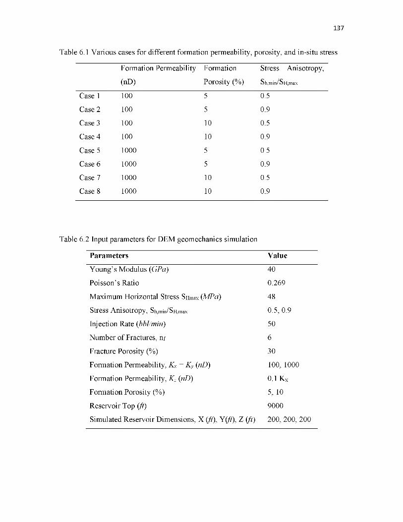
137

Table 6.1 Various cases for different formation permeability, porosity, and in-situ stress

Formation Permeability

(nD)

Formation

Porosity (%)

Stress Anisotropy,

Sh,min/SH,max

Case 1 100 5 0.5

Case 2 100 5 0.9

Case 3 100 10 0.5

Case 4 100 10 0.9

Case 5 1000 5 0.5

Case 6 1000 5 0.9

Case 7 1000 10 0.5

Case 8 1000 10 0.9

Table 6.2 Input parameters for DEM geomechanics simulation

Parameters Value

Young’s Modulus (GPa) 40

Poisson’s Ratio 0.269

Maximum Horizontal Stress SHmax (MPa) 48

Stress Anisotropy, Sh,min/SH,max 0.5, 0.9

Injection Rate (bbl/min) 50

Number of Fractures, nf 6

Fracture Porosity (%) 30

Formation Permeability, Kx = Ky (nD) 100, 1000

Formation Permeability, Kz (nD) 0.1 Kx

Formation Porosity (%) 5, 10

Reservoir Top (ft) 9000

Simulated Reservoir Dimensions, X (ft), Y ft), Z (ft) 200, 200, 200

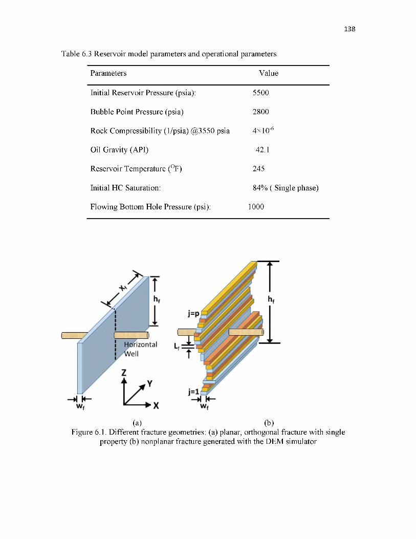
138

Table 6.3 Reservoir model parameters and operational parameters

Parameters Value

Initial Reservoir Pressure (psia): 5500

Bubble Point Pressure (psia) 2800

Rock Compressibility (1/psia) @3550 psia 4x10-6

Oil Gravity (API) 42.1

Reservoir Temperature (OF) 245

Initial HC Saturation: 84% ( Single phase)

Flowing Bottom Hole Pressure (psi): 1000

(a) (b)Figure 6.1. Different fracture geometries: (a) planar, orthogonal fracture with single

property (b) nonplanar fracture generated with the DEM simulator

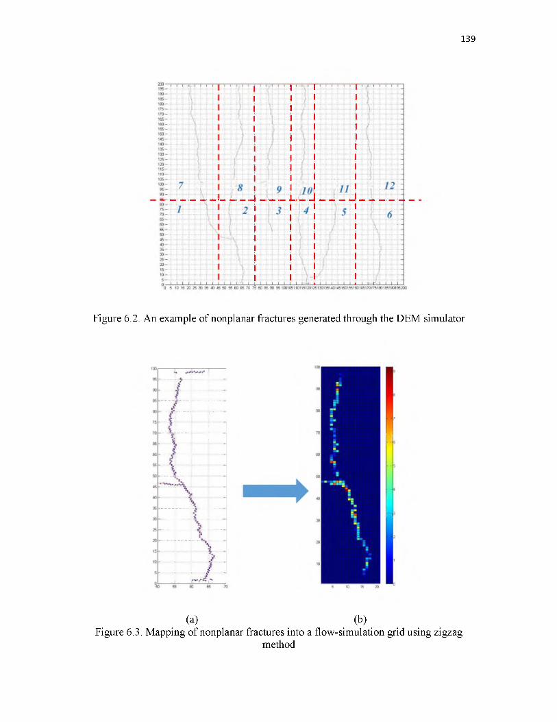
139

Figure 6.2. An example of nonplanar fractures generated through the DEM simulator

(a) (b)Figure 6.3. Mapping of nonplanar fractures into a flow-simulation grid using zigzag

method

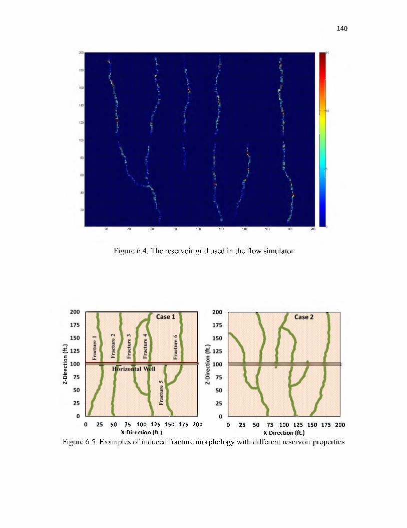
Z-D

irec

tion

(f

t.)

140

2 0 40 60 80 100 120 140 160 180 200

Figure 6.4. The reservoir grid used in the flow simulator

50 75 100 125 150 175 200 0 25 50 75 100 125 150 175 200X-Direction (ft.) X-D irection (ft.)

Figure 6.5. Examples of induced fracture morphology with different reservoir properties

141

0 25 50 75 100 125 150 175 200 X-Direction {ft.)

Figure 6.6. Schematic of fracture simplification of case 1

Figure 6.7. Comparison of oil recovery using the DEM model and simplified model forvarious cases

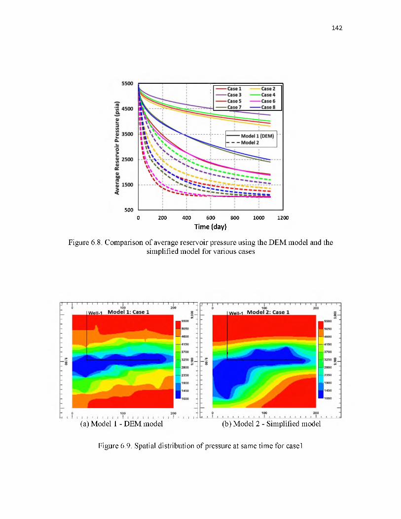
142

500 -------------------------------------*----------------- *-------------------------------------------------------

0 200 400 600 800 1000 1200

Time (day)

Figure 6.8. Comparison of average reservoir pressure using the DEM model and thesimplified model for various cases

(a) Model 1 - DEM model (b) Model 2 - Simplified model

Figure 6.9. Spatial distribution of pressure at same time for case1

C H A PT E R 7

DATA ASSIMILATION

Reservoir simulation is a valuable tool for predicting future reservoir performance and

optimizing oil and gas exploration. A numerical reservoir simulation model can describe

the fluid flow through porous media by applying rock and fluid property to a set of

mathematic equations (mass conservation and Darcy’s law). Therefore, whether the

simulation results are reliable or not largely depends on the accuracy of the formation

characteristics. Usually, reservoirs are buried thousands of feet below the surface, which

makes it impossible to directly and correctly measure all the parameters. But the rock

property fields can be constructed by applying inverse or parameter estimation algorithms

using indirect measurements, such as production data. In order to improve the predictive

capability, it is important to incorporate all relative information into a reservoir model, and

this process can be called data assimilation.

In this chapter, we are going to use Ensemble Kalman Filter (EnKF) to estimate and

update both the state variables (pressure and saturations) and uncertain reservoir

parameters (permeability). In order to directly incorporate spatial information such as

fracture location and formation heterogeneity into the algorithm, a new covariance matrix

method is proposed. Finally, this new method has been applied to a simplified single-phase

reservoir and a complex black oil reservoir with complex structures.

7.1 Introduction

In order to numerically simulate and solve different problems, a series of mathematic

equations are developed to describe the specific process. For dynamic processes, from time

tn-i to tn, the general discretized model equation can be written as:

x n = F (xn-1,6 ,u ) + w (7.1)

In the above equation, F is the nonlinear operator, 6 is model parameter, u is source or

sink term, n is the time step index, x is the state vector, w is model error or noise. Suppose

the measurements are only the function of states, then:

d = H(x) + v (7.2)

d represents the measurements, H is the output operator, v is the measurement noise.

From the mathematic point of view, a model is determined by parameters and states. In

order to get correct predictions, we need both the right model parameters and appropriate

model partial differential equations. However, for some applications, such as subsurface

reservoirs, the model parameters are invisible and contain large uncertainties, which will

cause bias in model calculations.

In past decades, data assimilation technology was widely used to estimate and update

the model dynamic variables while fixing the model parameters [109]. However,

considering the uncertainty that existed in model parameters, a state augmentation method

was proposed. The idea of augmented state (or Joint estimation [110]) is to estimate

uncertain model parameters jointly with the model states in the assimilation process [111].

The model parameters are added to the original state vector, and the equations for

parameters updating are combined with the model equations. Then the conventional

assimilation algorithm is applied to this new augmented system [112]. In other words, the

144

augmented state method transforms the state and parameter estimations into traditional

parameter estimations by incorporating the parameter into the state vector. This augmented

state can reduce the uncertainty in both model parameters and dynamic variables; therefore

it has been widely used in many areas.

There are many different ways to classify the large number of estimators. Here, we

categorize all data assimilation methods into two groups. The first group is nonrecursive

method, also called batch processing or off-line estimator method [113]. The batch

processing algorithm requires storage of all historical data and processes them at one time

step [114]. In order to examine the performance of the updated/estimated parameters, the

researchers separate the whole set of data into two parts, one is for identification of

parameters, and the other one is for verification of results. Since this algorithm processes

all data at one step, it is easy to implement. However, it lacks the flexibility to examine the

evolution of model parameters, and it is not able to incorporate new information.

Recursive method is the other type of data-assimilation method. Compared with the

batch group, the recursive method can continuously update the augmented state vector with

the newly observed data. The recursive estimator utilizes the prior estimates as a starting

point for a sequential estimation algorithm [115]. From this point of view, we can regard

the batch estimator as the first step in a recursive estimator.

The parameter and state estimations can also be treated as an optimization problem.

For optimization, one of the primary problems required to be solved is the choice of the

best function, which means the objective functions to be minimized or maximized [116].

A least- squares method (LSM) [117] is a popular way to do parameter estimation. It aims

at minimizing the sum of squares of the difference between data and predicted

145

measurements. There are also methods based on the statistical theory and probability

density function. One of the commonly used estimators is the Bayes estimator, which

minimizes the posterior expected value of a loss function [118]. In this method, the prior

distribution of the model parameters is assumed to be known in advance and the widely

used risk function is the mean square error. Another popular estimator is maximum

likelihood estimator (MLE) [119], [120], which is based on the idea of maximizing the

probability density of observed measurements through the estimation of parameters [121].

The primary difference between MLE and least squares is that MLE requires a normal

distributed error. Although the maximum a-posteriori estimation is closely related to the

maximum likelihood method, it has an augmented optimization objective, which examines

not only the difference between predicted results and the observations but also the deviation

of updated parameters from the prior distribution [122].

A Kalman filter (KF) is another kind of recursive parameter-state estimator based on

Bayes theory. The Kalman filter [123] is an algorithm that utilizes a series of perturbed or

inaccurate observations to identify unknown variables. The traditional Kalman Filter is

recognized as an optimal estimator for linear system because it can minimize the mean

square error of the estimated parameters if all noise is Gaussian. The Kalman filter has

many advantages compared with other estimators: good estimation results, capability for

online real-time processing, easy to implement, and no need for the inversion of

measurement equations. However, it is not suitable for nonlinear system [124]. Because

there is no perfect linear system in reality, the Extended Kalman Filter (EKF) [125] is

proposed to project the idea of the Kalman Filter into a nonlinear system. The EKF utilizes

Taylor expansion to approximate the nonlinear term. Therefore, EKF can deal with some

146

simple nonlinear systems, but does not perform well in highly nonlinear models. In

addition, it becomes infeasible for large-scale systems due to the calculation of the

sensitivity matrix. In order to overcome the limitations of EKF, a Monte Carlo-based

Ensemble Kalman Filter (EnKF) was proposed in 1994 [126]. The EnKF was first used in

oceanology and weather prediction. In 2002, the EnKF was introduced to estimate reservoir

parameters and states [127]. Compared with the traditional Kalman filter and extended

Kalman filter, the EnKF can cope with a highly nonlinear system without linear

approximation of nonlinearities [128]. It also has many other advantages, such as a small

computational load, convenience of coupling with different simulators, a relatively simple

method for assessing the uncertainty of state variables, and applicability to large-scale

models [129].

Moving Horizon Estimation (MHE) is also an optimization-based estimator [130].

Unlike the previously mentioned state estimators which use the most recent measurement

or the whole measurements to update the model parameters and states, the MHE utilizes a

fixed amount of data to do the estimation [131]. The fixed length of time interval is called

the horizon. Therefore, it can improve the efficiency of computation and avoid some

unreasonable parameter estimation to a certain degree. In addition, compared with other

estimators which are also based on statistics theory, the MHE can deal with non-Gaussian

types of noise and prior distribution, which is a big constraint for Kalman Filter

applications [132]. But one main deficiency of the MHE is the definition of the arrival cost

that is the effect of “old data” on the further updating processs. Moreover, the uncertainty

analysis is hard to implement in the MHE.

One important feature of MHE is allowing the utilization of constraints in the algorithm

147

[133]. In MHE, researchers can limit the changing of model parameters and state updates

by defining the possible ranges. This idea of constraints is especially useful for avoiding

some unrealistic estimations from data assimilation and inversion algorithms. In Kalman-

filter-related methods, the equality constraints have been incorporated and investigated in

many articles [134]—[137]. The inequality constraints which are more meaningful for data

assimilation were further developed based on the equality constraints [138]. The idea of

inequality constrains has combined with EnKF through the adoption of Lagrange

multipliers [139]. Although those methods can provide some help in model parameter

estimation, they do not directly reflect the parameter characteristics. One typical example

is the identification of reservoir permeabilities. For the highly uncertain reservoir, the

determination of the permeability field is crucial in predicting oil production. There are

factures and faults existing in the reservoir which may prompt or inhibit the flow of

hydrocarbons, as shown in Figure 7.1. In this figure, the block represents a reservoir and

the red zone in the middle of the reservoir is a channel with high permeability.

Undoubtedly, the production prediction from the numerical flow simulator will be greatly

different from the observations if this high permeability zone is ignored.

By using the methods mentioned before to update the permeability of this reservoir with

the prior knowledge about the boundary of this channel, the constraint should be set up for

all the points encircled by the boundary which needs not only highly efficient

computational tools but also an appropriate choice of the constraint value. In this section,

we propose a method to deal with the problem of updating model parameters with spatial

structure on the basis of an Ensemble Kalman Filter. According to the spatial

characteristics, we add a covariance term, which could be regarded as the representation of

148

uncertainty of the model parameters. Adding this term does not increase the computation

burden much and exhibits better parameter estimation.

The goal of using an augmented state vector is to estimate the model parameters as well

as dynamic variables and reduce the parameters’ uncertainties. For these applications

where spatial structure has significant effects on the predictions, such as reservoir

simulation, none of those existing methods can directly incorporate the structure

information into the estimation process. The innovation of this research is that the model

parameter estimation will be improved by utilizing prior knowledge about the spatial

structure.

The chapter is organized as follows. In Section 7.2, the procedure of implementing

EnKF is illustrated. And the proposed method, covariance matrix method, is demonstrated

in Section 7.3. In Section 7.4, two examples (single-phase reservoir and complex black oil

reservoir) are used to verify the viability of the proposed idea.

7.2 The Algorithm of Ensemble Kalman Filter

The Ensemble Kalman filter is a very popular and promising method for improving and

calibrating the reservoir model to match production data in recent years. This method can

be separated into two steps: a forward step and an update step. In the forward step, the state

propagates from tn-i to tn, and in the update step, the state is updated through assimilating

measurement data. It is expected that the updated state shows better match with the true

state vector. Figure 7.2 is the flowchart of implementing EnKF.

Each ensemble is an augment vector. Usually, the augment state vector consists of three

parts: 1) uncertain static model parameters (m) such as permeability and porosity, 2)

149

150

dynamic variables (5) such as pressure and saturation, and 3) production data (d), including

well production rate, bottom hole pressure, water cut, gas oil ration, and so on. So, in

general, the state vector we used in EnKF is

Due to the fact that the EnKF is a sequential Monte Carlo method, the initial ensemble

x0 is generated as a Gaussian random field. The spread of the ensembles represents the

uncertainty of the state. Geophysical logs and other measurements can be used to estimate

the initial permeability field.

From Equation (7.1), the forward state after time propagation is

wherej is the index of ensemble, Ne is the total number of ensembles, Wj is the model error

of each ensemble, which is independent of state vector and is supposed to be a Gaussian

distribution with zero mean and covariance matrix ¥ . According to Zupanski’s paper

[140], while applying the Ensemble Kalman Filter, the model error term can directly affect

the performance of EnKF and may lead to filter divergence if neglected. Superscript f

means forward state after time propagation, while a indicates analysis state after data

assimilation.

Observations can be treated as random variables or deterministic values. In here,

according to Burgers’s paper [141], we set the measurements as a stochastic number

incorporated in the state vector, so the output operator H is a matrix with only zeros and

x = s -d

(7.3)

Xh,j = F(.xZ-l,j' u ) + wj ’ j = l , -"> Ne (7.4)

(7.5)

^observation is given by Equation 7.2. Since the production data have already been

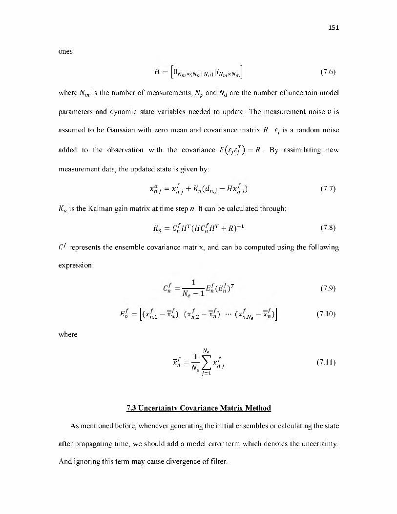
151

ones:

H = [°WmX(Np+Nd)|/wmXNm] (7.6)

where Nm is the number of measurements, Np and Nd are the number of uncertain model

parameters and dynamic state variables needed to update. The measurement noise v is

assumed to be Gaussian with zero mean and covariance matrix R. Ej is a random noise

added to the observation with the covariance E (ejeJ ) = R . B y assimilating new

measurement data, the updated state is given by:

xn,j = xi j + Kn(dn,j - H x ^

Kn is the Kalman gain matrix at time step n. It can be calculated through:

Kn = c lH T(H ClH T + R )-1

(7.7)

(7.8)

C? represents the ensemble covariance matrix, and can be computed using the following

expression:

?fruf\T

E-n = [(*n,1 xnV (xn,2 xn} (xn,Ne xn̂ )]

(7.9)

(7.10)

where

NP

* = i i *e j=i

(7.11)

7.3 Uncertainty Covariance Matrix Method

As mentioned before, whenever generating the initial ensembles or calculating the state

after propagating time, we should add a model error term which denotes the uncertainty.

And ignoring this term may cause divergence of filter.

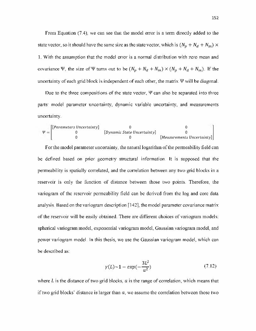
From Equation (7.4), we can see that the model error is a term directly added to the

state vector, so it should have the same size as the state vector, which is (Np + Nd + Nm) x

1. With the assumption that the model error is a normal distribution with zero mean and

covariance V, the size of V turns out to be (Np + Nd + Nm) x (Np + Nd + Nm) . If the

uncertainty of each grid block is independent of each other, the matrix V will be diagonal.

Due to the three compositions of the state vector, V can also be separated into three

parts: model parameter uncertainty, dynamic variable uncertainty, and measurements

uncertainty.

152

[Parameters Uncertainty] 0 00 [Dynamic State Uncertainty] 00 0 [Measurements Uncertainty]

For the model parameter uncertainty, the natural logarithm of the permeability field can

be defined based on prior geometry structural information. It is supposed that the

permeability is spatially correlated, and the correlation between any two grid blocks in a

reservoir is only the function of distance between those two points. Therefore, the

variogram of the reservoir permeability field can be derived from the log and core data

analysis. Based on the variogram description [142], the model parameter covariance matrix

of the reservoir will be easily obtained. There are different choices of variogram models:

spherical variogram model, exponential variogram model, Gaussian variogram model, and

power variogram model. In this thesis, we use the Gaussian variogram model, which can

be described as:

3L2 tn ..y ( L ) ~ 1 - e x p ( ----- 5-) (712)

a2

where L is the distance of two grid blocks, a is the range of correlation, which means that

if two grid blocks’ distance is larger than a, we assume the correlation between those two

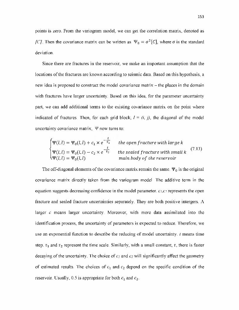
points is zero. From the variogram model, we can get the correlation matrix, denoted as

[C ]. Then the covariance matrix can be written as ¥ 0 = o 2[C], where a is the standard

deviation.

Since there are fractures in the reservoir, we make an important assumption that the

locations of the fractures are known according to seismic data. Based on this hypothesis, a

new idea is proposed to construct the model covariance matrix - the places in the domain

with fractures have larger uncertainty. Based on this idea, for the parameter uncertainty

part, we can add additional terms to the existing covariance matrix on the point where

indicated of fractures. Then, for each grid block, l = (i, j), the diagonal of the model

uncertainty covariance matrix, ¥ now turns to:

{¥ (1 ,1) = ¥ 0(l, I) + cl x e xi the open fra c tu re w ith large k

, — (713)

¥ ( l , I) = ¥ 0(l, I) — c2 x e r 2 the sealed fra c tu re w ith sm all k¥ ( l , I) = ¥ 0(l, I) m ain body o f the reservo ir

The off-diagonal elements of the covariance matrix remain the same. ¥ 0 is the original

covariance matrix directly taken from the variogram model. The additive term in the

equation suggests decreasing confidence in the model parameter. ci,c2 represents the open

fracture and sealed fracture uncertainties separately. They are both positive intergers. A

larger c means larger uncertainty. Moreover, with more data assimilated into the

identification process, the uncertainty of parameters is expected to reduce. Therefore, we

use an exponential function to describe the reducing of model uncertainty. t means time

step. t 1 and x2 represent the time scale. Similarly, with a small constant, t , there is faster

decaying of the uncertainty. The choice of ci and C2 will significantly affect the geometry

of estimated results. The choices of cx and c2 depend on the specific condition of the

reservoir. Usually, 0.5 is appropriate for both cx and c2.

153

There is no doubt that the predefinition of the fracture location plays a crucial role in

estimating the static parameters of the reservoir. However, if the location and shape

information about the reservoir fracture are not precisely known already, then both

orientation and permeability have certain uncertainties. Therefore, we need to modify the

whole process. The basic idea is to do multiple estimations and choose one of the best from

these identifications. First, even without an accurate picture, it is reasonable to assume that

the location and orientation of the fractures are roughly known based on the seismic data.

Thus, several possibilities about fracture geometry can be assumed. Using each of those

guesses and applying it into the EnKF algorithm with the same observation, the different,

updated permeability field can be obtained separately. After that, we need to choose the

optimal distribution from the updated results. There are two ways to evaluate the updated

results:

1) Use the updated parameters in the reservoir model instead of the prior one, run

the simulation, then compare the simulation results with the observation; the one

with the minimum difference is the best estimation.

2) Check the predictions from the updated permeability. Sometimes, the predictions

from uncorrected updated distributions will lead to strange or unreasonable

production profiles and inconsistency with the previous observations. The model

shows the best consistency is the optimal choice.

We can use both of the methods to decide which one is the best estimation. In certain

conditions, if the guess of the fracture is too far from the true situation, only method 2 is

enough to make the correct decision. Even if the precise knowledge about the fractures is

known, those two criteria can also be used to examine the quality of the estimation.

154

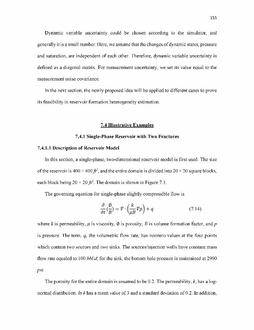
155

Dynamic variable uncertainty could be chosen according to the simulator, and

generally it is a small number. Here, we assume that the changes of dynamic states, pressure

and saturation, are independent of each other. Therefore, dynamic variable uncertainty is

defined as a diagonal matrix. For measurement uncertainty, we set its value equal to the

measurement noise covariance.

In the next section, the newly proposed idea will be applied to different cases to prove

its feasibility in reservoir formation heterogeneity estimation.

7.4.1.1 Description of Reservoir Model

In this section, a single-phase, two-dimensional reservoir model is first used. The size

of the reservoir is 400 x 400f t2, and the entire domain is divided into 20 x 20 square blocks,

each block being 20 x 20f t2. The domain is shown in Figure 7.3.

The governing equation for single-phase slightly compressible flow is

where k is permeability, ^ is viscosity, 0 is porosity, B is volume formation factor, and p

is pressure. The term, q, the volumetric flow rate, has nonzero values at the four points

which contain two sources and two sinks. The sources/injection wells have constant mass

flow rate equaled to 100 bbl/d; for the sink, the bottom hole pressure is maintained at 2900

psi.

The porosity for the entire domain is assumed to be 0.2. The permeability, k, has a log-

normal distribution. In k has a mean value of 3 and a standard deviation of 0.2. In addition,

7.4 Illustrative Examples

7.4.1 Single-Phase Reservoir with Two Fractures

there are two fractures in the reference model, which is used to reflect the reality, one is an

open fracture with k equal to 10,000 md, and the other one is a sealed fracture, in which k

equals to 0.001 md. The log-permeability field is shown in Figure 7.4.

7.4.1.2 With Accurate Knowledge of Fractures

In order to examine the performance of EnKF in updating the static parameters

(permeability) and dynamic variables (pressure), two models will be used: a true model

and a biased model. The true model, which has the right initial conditions and perfect prior

knowledge of the reservoir characteristics, provides measurements to the biased model. We

assume that the detailed information about the true model is not available and use the biased

model with imperfect knowledge. The distinctions between the true model and biased

model include initial pressure and permeability. At t=0s, both the true and biased model

are assumed to have uniformly distributed pressure equal to 3000psi in the true condition.

The pressure difference between the two models is nearly 4%. The permeabilities in both

of the models are generated using Gaussian random variables with the same mean and

covariance. However, there are two fractures located at (10:18, 5) and (2:12, 2) in the true

model which do not exist in the biased one. The comparison of the two models used in the

section is shown at Figure 7.5. Our goal is to estimate the fracture properties by providing

measurements.

As mentioned before, there are four wells in the reservoir, which are located at (1, 1),

(5, 15), (15, 5), and (20, 20). In addition to the four wells, there are two more monitoring

wells, (12, 5) and (17, 5), to measure the pressure changes. In order to minimize the

negative effects brought by an insufficient number of ensembles, we set the ensemble size

156

While applying EnKF in the reservoir model we assume that the following quantities

are available: bottom hole pressure and fluid production rate. For the injectors which are

kept at constant flowrate, the bottom hole pressure is the measurements. For the producer

with bottom hole pressure constraint, the production rate is the measurement. And the terms

that are tuned with the Ensemble Kalman filter are the permeability and pressure of each

grid block. The uncertainty of measured pressure is 10 psi, and the uncertainty of the

production rate is 1 bbl/d.

After determining the uncertainty of measurements, the model uncertainty is another

factor to be decided. The prior knowledge of the fracture location is a key assumption to

identify fracture permeabilities in this section. According to the definition in Section 7.3,

location of fracture has larger uncertainty than the main matrix, we can set ci equal to 1 at

open fracture (10:18, 5), and C2 equal to 0.5 at sealed fracture (2:12, 2). The other elements

in the covariance matrix kept the same with the previous one while generating the initial

distribution. The time scale, t 1 and t 2 , are set to 20 to make sure that the model uncertainty

will not decrease too fast.

Due to the fact that the only dynamic variable in single-phase flow is pressure, and the

pressure change of each grid block is independent, the dynamic variable uncertainty block

is set as a diagonal matrix with the diagonal equal to 20 psi. This value is constant, since

this uncertainty derives from the model itself. The whole simulation time is 200 days. The

first 100 days are the updating period, with one set of data for each day. The following 100

days are the predicting period, which the model runs with updated permeability and

pressure.

157

equal to 200.

The evolutions of the permeability estimation and update, are shown in Figure 7.6. As

mentioned before, the main difference between the two models is the presence of fractures.

Initially, no fractures exist in the biased model. With more data incorporated in the process,

the fractures are gradually estimated. After 100 data assimilation, the fractures are correctly

captured based on the biased model.

From those figures, we can find that during the whole assimilation process, the first

few steps play a more important role in adjusting the model static parameter compared with

the later cycles. As time goes on, the value of uncertainty decreases, therefore the spread

of the ensembles is reduced, and measurements’ profiles become flatter, so their

contribution to the estimation is diminished.

In addition, the cycles needed to identify fractures are not the same. For the open

fracture, which has large permeability, it takes only 5 cycles to obtain the correct

permeabilities and shape of the fracture in this example. On the contrary, for the sealed

fracture, the time increases to 40. The possible reasons for this disparity are: 1) there are

three measurements located at the open fracture (12, 5), (15, 5), and (17, 5). Those

measurements are quite sensitive to the permeability change. 2) there are no measurements

which could directly reflect the pressure change of the sealed fracture, and a sealed fracture

is a place where pressure is nearly constant. Thus, more steps are required to correctly

update the permeability distribution. Therefore, the factures which are more sensitive to

measurements are more easily to be identified. And the information contained in the

measurements will influence the accuracy and efficiency of the identification process.

In addition, four points from the reservoir are chosen to illustrate the evolution of

permeability with time. Point (a) and (b) are located at the open fracture, point (c) is in the

158

sealed fracture, and (d) is an arbitrary point taken from the main matrix. Figure 7.7

illustrates the updating process about the permeability of these points.

From Figure 7.7, we can see that after several cycles, the permeabilities of those points

have achieved a steady state, which proves the stability of this EnKF system. Moreover,

the (a) and (b) points reach high value at first, and then decrease to a constant value. The

high value appearing at the beginning is due to the large uncertainty value we used in the

example (ci = 1). The point (c) keeps decreasing at a relatively low pace to its objective,

compared with point (a) and (b). Due to the low uncertainty of the main body, the

permeabilities of internal points do not have significant changes. Those results are in

accordance with the pervious analysis.

Next, the effects of EnKF brought to the outputs is examined. Figure 7.8 is the profiles

of the true solution, biased solution, measurements, and estimated solution from the

Ensemble Kalman filter for different measured quantities. The total simulation time is 200

days. The vertical dashed line separate the whole simulation time into updating period and

predicting period.

Figures 7.8 (a) and (d) show the bottom hole pressure of the two injectors. (b) and (c)

are the fluid production rate of the two producers. (e) and (f) are the bottom hole pressure

of the monitoring wells.

From those figures, we can first see that the outputs from the biased model are greatly

different from the observations due to missing fractures and incorrect initial pressure in the

model, especially in the flowrate of well 2 and well 3. Among all those six pictures, the

outputs from the biased model are higher than the true model except for well 3. The reason

for this phenomenon is that a higher initial value is used in the biased model. Since the

159

reservoir model used in this section is single-phase and homogeneous-field, the higher

initial pressure will lead to an increased pressure at each well during the whole simulation

time. Well 2 is located in the middle of the reservoir, so its flowrate is primary dependent

on the pressure of its grid block and its neighborhood. Therefore, the output of well 2 in

the biased model is also larger than the true model. On the contrary, well 3 is located at the

open fracture with high conductivity so that the flow rate in the true model is much larger.

However, in the biased model, there is no fracture, and the flowrate is a relatively small.

After applying EnKF in the biased model, the estimations can match the observed

measurements during the updated period. And after 100 days of assimilation, the forecast

from the updated reservoir model follows the true curves closely. Thus, the EnKF can

correct the deviation caused by the unknown static parameters and the initial conditions in

the biased model.

The pressure distributions of the whole domain from the true, biased, and updated

models are shown in Figure 7.9 and 7.10. With the presence of open fracture in the true

model, there is a low-pressure zone at the right bottom corner because of the hydrocarbon

production. The existence of a low-permeability fault leads to slightly changed pressure

around the fault. By comparing Figure 7.9 (a) and (b), it is obvious that without considering

the fractures and high initial pressure, the pressure of the biased model at the final

simulation time (t = 200 days) is symmetrically distributed and significantly deviated from

the true case.

Figure 7.10 is the pressure distribution with updated permeability at time t = 200 days.

Comparing Figure 7.10 with the true case (Figure 7.9(a)), the pressure is almost the same.

Only some points at the seal fractures cannot be precisely captured.

160

7.4.1.3 Without Accurate Knowledge of Fracture Location

In this subsection, the case with uncertainties in both the orientation and permeability

of the open fracture is investigated. The reservoir model mentioned in Section 7.4.1.1 is

used here. The model is two-dimensional, single-phase, slightly compressible reservoir

with 4 wells and 2 monitoring wells. We expect to get an estimation similar to the true field

after the observations’ assimilation.

As with the example in Section 7.4.1.2, there are also two models, the true model and

the biased model. The open fracture in the true model is located at (10:18, 5), and no open

fracture is in the biased model. Since we do not have the exact picture of the location or

the shape of the fracture, we need to make some hypothesis of the facture’s characteristics.

Based on the seismic data, we make the following seven assumptions of possible open

fracture location and shape:

(1) Exactly the right location, (10:18, 5).

(2) One gridblock upper, (10:18, 6).

(3) One grid block lower (10:18, 5).

(4) With small positive slope (slope » 1/2).

(5) With small negative slope (slope » -1/2).

(6) With large positive slope (slope » 1).

(7) With large negative slope (slope » -1).

According to these possible locations of the facture, we can define different model

uncertainty covariance matrixes. The composition of the matrix varies with the assumed

location and shape of the fracture. Applying the specific covariance matrix to the Ensemble

Kalman Filter, seven estimated distributions of permeabilities can be obtained with the

161

same observations. The figures of seven different updated estimations show in Figure 7.11.

The shape of the identified fracture is strictly determined by the previously defined

fracture orientation. Since we only examine the identifying process of the open fracture,

the sealed fracture is fixed. And due to the small uncertainty of the main matrix of the

reservoir, their permeabilities do not have obvious differences.

After obtaining those figures, we need to choose the optimal estimations from all those

choices. As mentioned before, there are two methods which can help find the correct shape:

(1) Substitute the previous biased permeability with the updated one, and examine the

difference between the estimated output and observations.

(2) Check the prediction after the updating process, the model with incorrect

distribution may produce some unreasonable profiles.

In here, we first use method 2 because of the small computational load. Table 7.1 shows

the last outputs from six wells after updating compared with the first predictions without

updating.

From Table 7.1, it can be noticed that compared with pressure, the flowrates of well 2

and 3 show larger changes between the last updated and first predicted outputs. The

pressure differences among different cases are almost the same. Therefore, in this example,

flowrate is a better indicator of the correctness of the estimated results.

Checking the flowrate, case 2 (moving upward), case 3(moving downward), case 6

(with large positive slope), and case 7 (with large negative slope) exhibit significant

inconsistence in predictions after 100 cycles of updating. The first predictions of flowrate

after data assimilation are less than or close to zero. Clearly, those four assumptions of the

fracture location are not as accurate as the other three assumptions. And among the other

162

163

three cases, case 1 (the true location) shows a smaller difference between the last updating

with the first prediction than case 4 (with small positive slope) and case 5 (with small

negative slope). Therefore, in all seven cases, case 1 has the most precise assumption about

the location and orientation of the open fracture, and it shows the best consistency. Case 4

and Case 5 are closely similar to the true situation, and the results are better than the other

4 cases.

In addition, we can see “symmetric effect” from the table. For example, case 2 and case

3 are symmetric in the position, so the deviations of the prediction from the observation

are pretty close. This is also true for case 4 and case 5, case 6 and case 7. This “symmetric

effect” also brings some hints for identifying the location of the fracture. If some similar

deviations or inconsistencies between the prediction and observation are observed, the

fracture’s correct shape may be in the middle of those two situations.

From the analysis based on method 2, we can make the judgment that case 1 is the best

result among all the seven possibilities. Now, method 1 is utilized to verify this statement.

The way of implementing method 1 is by applying the updated permeability into the biased

model. So this new model has updated static parameters (permeability) and biased initial

conditions (P = 3100 psi). Comparing the prediction from the new model with observations,

the one with smallest root mean square (RMS) error is the optimal choice.

The “Initial” column represents the error between true situation and original biased

model without any data assimilation. Due to the incorrect initial value and lack of fractures

presented in the original biased model, the RMS error is very large. All cases show reduced

error after incorporating EnKF in the algorithm, even the situations with inaccurate fracture

location assumption. But because of the biased initial conditions, RMS error is not that

small after data assimilation.

Analyzing each of the cases, the conclusions obtained through method 1 are in

accordance with the method 2 results. Case 1 is the best case because of the minimum error.

The RMS errors of case 4 and case 5 are better than other cases.

There are also “symmetric effects” in the error calculation. Cases 2 and 3, cases 4 and

5, and cases 6 and 7 show certain similarity in RMS error. In addition, compared with the

assumption made in cases 4 and 5, which is a small angle deviated from the true solution,

cases 6 and 7 base on a more unrealistic assumption of large angle of fracture, so the error

of cases 6 and 7 is larger than that of cases 4 and 5. This phenomenon provides insights

into assumptions about the fracture characteristics at the very beginning step. For example,

in case 1 and case 2, if two locations of the open fracture are assumed, case 2 should be

one grid block further than case 1 in y direction. After obtaining the RMS error of those

two cases, it can be found that case 2 produces larger error. Therefore, it is not necessary

to try those hypothetical cases with locations even higher than case 2 in y direction. The

error keeps increasing with the increasing deviation from the true situation. Through this

criterion, the computational load is greatly reduced.

From those two tables, it can be proved that these two methods can provide some

guidance in choosing a model among different realizations. Furthermore, considering the

non-uniqueness of EnKF updating results, and in order to get more accurate description of

the reservoir and also reduce the side effects brought by the random number, the whole

simulation can be repeated several times, and the estimations from all results averaged.

164

7.4.2 Three-Phase Black Oil Reservoir - PUNQ-S3 Model

The performance of the proposed idea about EnKF with covariance matrix was also

examined in the well-known PUNQ-S3 reservoir model. The PUNQ-S3 model is a three-

phase black oil model with 19 x 28 x 5 grids, of which 1761 blocks are active. The top

structure of the reservoir is shown in Figure 7.12.

There is a strong aquifer located at the north-west corner and a small gas cap existed in

the center of the reservoir. During the primary production, there are only 6 production

wells. When entered into the secondary production period, 5 injection wells will be added.

In this paper, we only consider the situation with 6 production wells.

In order to simply implementation, each well will produce at a constant flow rate equal

100 m3 of oil per day. The lower limit of well bottom hole pressure is 120 bar. The total

simulation time is 2 years, and one set of data can be obtained at the end of each month.

Therefore, 23 series of production data will be available in total. Each set of measurement

data consists of bottom hole pressure and gas/oil ratio from all production wells.

According to the description of this PUNQ-S3 model [143], the five layers exhibit large

geological heterogeneities. Layers 1, 3, and 5 consist of fluvial channels embedded in a

low, porous, floodplain mudstone. Layer 2 represents marine or lagoonal clay. Lay 4

contains mouthbars or lagoonal deltas within lagoonal clays. The geological composition

of this small scaled reservoir provides information needed in EnKF with covariance matrix

method.

Compared with the traditional EnKF algorithm, one advantage of EnKF with

covariance matrix is the ability to incorporate geological information into the modeling

and obtain better estimated results by assimilating the measurement data. Thus, the PUNQ-

165

S3 model, especially the layers with the channels, is a suitable case to apply the covariance

matrix method. We took the first layer as an example. Supposing the locations of high

permeability streaks are known, we can organize the covariance matrix according to the

method mentioned in Section 7.3. The updated permeability field is shown in Figure 7.13.

Figure 7.13 (a) is the reference permeability field of the first layer. (b) is the initial

permeability combined with EnKF. (c) and (d) represent the updated permeability at

different time steps. The black circles are production wells.

The inversion process started from an uniformly distributed permeability field

within k « 5 . The heterogeneity of the channels is not present initially. After assimilating

the first 12 sets of measurement data (Figure 7.13 (c)), the shape of the two streaks can be

identified, although not very accurately. At the final step, the updated permeability field

almost matches the reference one. However, the low permeability area (colored as dark

blue) at the west boundary was not precisely updated due to the lack of a production well

in that area. No measurements can directly reflect the geological property of that area. This

problem can be solved if more wells are added in that area.

If knowledge about the streak is not included in EnKF, the updated permeability field

with a conventional EnKF algorithm is shown in Figure 7.14.

Comparing Figure 7.14 with Figure 7.13, it is obvious that if the traditional EnKF

without covariance matrix is used for updating permeability, 3 high-permeability channels

appeared after 23 data assimilations. The locations with low permeability cannot be

identified, either.

Figure 7.15 is the predicted bottom hole pressure of well 5 from the initial permeability

field and updated permeability field. The grey lines represent the BHP predictions from all

166

ensembles. The green line is the mean value of all ensembles and the red line is the

observation data. Figure 7.15(a) is the prediction from well 5 with initial permeability

ensembles. And Figure 7.15(b) is the prediction with updated permeability ensembles.

After assimilating production data, the spread of ensemble predictions is greatly decreased,

which means that the uncertainty of predictions is greatly reduced, and the mean values of

all updated ensembles are nearly equal to the correct value. This case proves that EnKF

with covariance matrix can improve reservoir parameter estimation.

7.5 Summary

The reservoir is a subsurface pool and cannot be entirely visible to researchers. The

uncertainty and biased reservoir parameters will lead to very different performance

predictions even under the same operation condition, especially for the reservoir with

fractures and heterogeneity. The methodology of the Ensemble Kalman Filter (EnKF)

addresses this issue led by biased model parameters through appropriate incorporation of

different kinds of data, such as production and pressure from wells. The model prediction

is improved and the parameters used to describe formation are better defined with reduced

uncertainty after the data assimilation process. Moreover, by proposing the novel

covariance matrix method for describing the model parameter uncertainty, the spatial

information of the reservoir is directly incorporated into the algorithm. From the simulation

results, both the fracture properties (orientation and permeability) and formation

heterogeneity can be better captured.

167

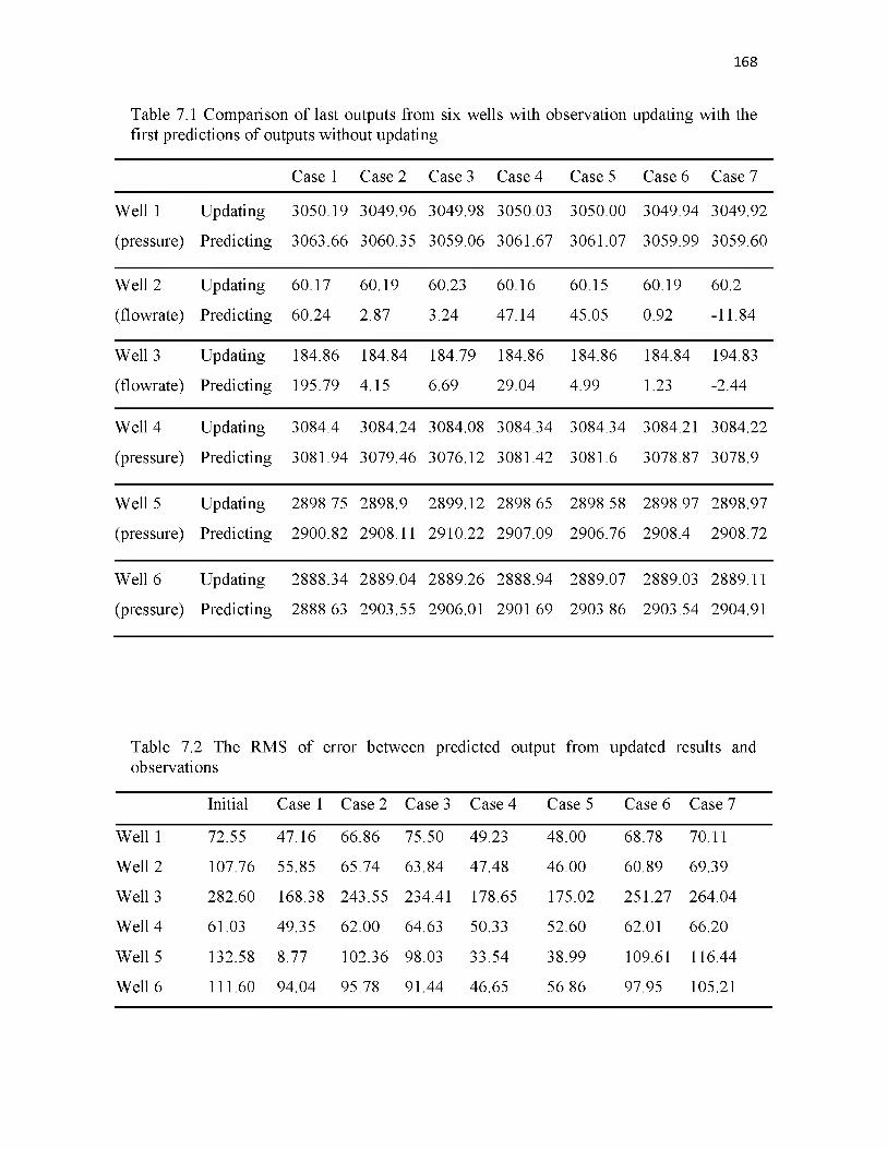
168

Table 7.1 Comparison of last outputs from six wells with observation updating with the first predictions of outputs without updating

Case 1 Case 2 Case 3 Case 4 Case 5 Case 6 Case 7

Well 1

(pressure)

Updating

Predicting

3050.19

3063.66

3049.96

3060.35

3049.98

3059.06

3050.03

3061.67

3050.00

3061.07

3049.94

3059.99

3049.92

3059.60

Well 2

(flowrate)

Updating

Predicting

60.17

60.24

60.19

2.87

60.23

3.24

60.16

47.14

60.15

45.05

60.19

0.92

60.2

-11.84

Well 3

(flowrate)

Updating

Predicting

184.86

195.79

184.84

4.15

184.79

6.69

184.86

29.04

184.86

4.99

184.84

1.23

194.83

-2.44

Well 4

(pressure)

Updating

Predicting

3084.4

3081.94

3084.24

3079.46

3084.08

3076.12

3084.34

3081.42

3084.34

3081.6

3084.21

3078.87

3084.22

3078.9

Well 5

(pressure)

Updating

Predicting

2898.75

2900.82

2898.9

2908.11

2899.12

2910.22

2898.65

2907.09

2898.58

2906.76

2898.97

2908.4

2898.97

2908.72

Well 6

(pressure)

Updating

Predicting

2888.34

2888.63

2889.04

2903.55

2889.26

2906.01

2888.94

2901.69

2889.07

2903.86

2889.03

2903.54

2889.11

2904.91

Table 7.2 The RMS of error between predicted output from updated results and observations

Initial Case 1 Case 2 Case 3 Case 4 Case 5 Case 6 Case 7

Well 1 72.55 47.16 66.86 75.50 49.23 48.00 68.78 70.11

Well 2 107.76 55.85 65.74 63.84 47.48 46.00 60.89 69.39

Well 3 282.60 168.38 243.55 234.41 178.65 175.02 251.27 264.04

Well 4 61.03 49.35 62.00 64.63 50.33 52.60 62.01 66.20

Well 5 132.58 8.77 102.36 98.03 33.54 38.99 109.61 116.44

Well 6 111.60 94.04 95.78 91.44 46.65 56.86 97.95 105.21

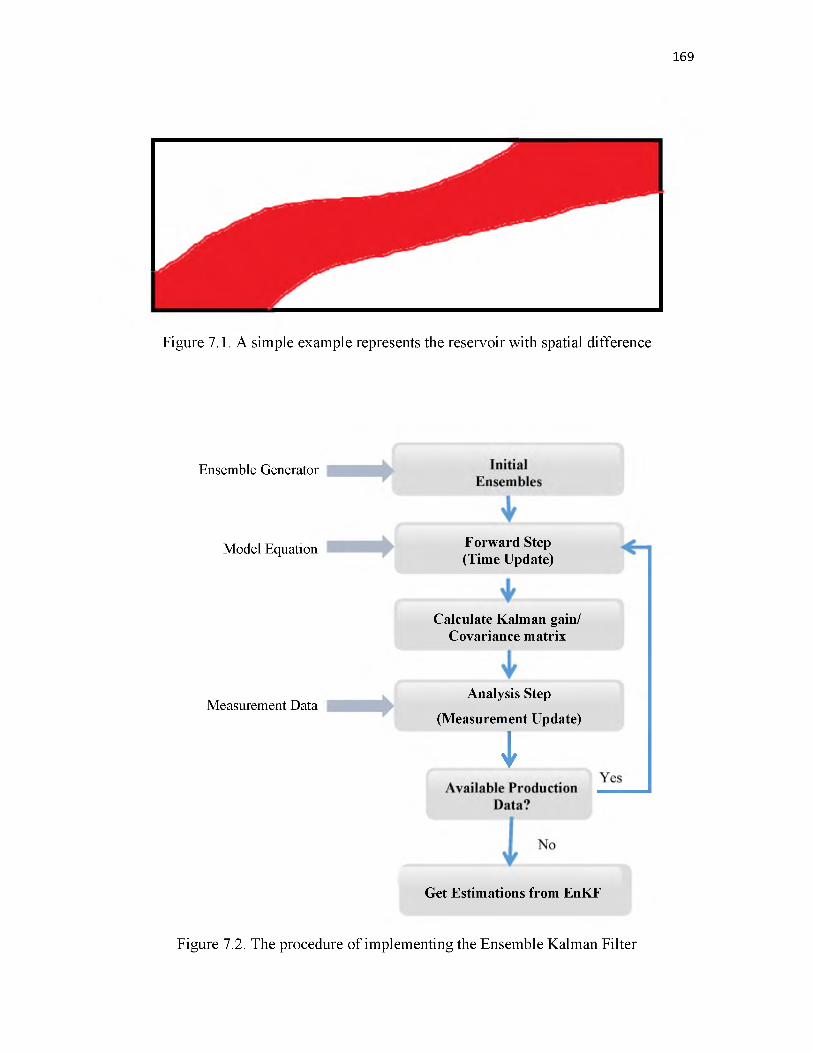
169

Figure 7.1. A simple example represents the reservoir with spatial difference

Ensemble Generator

Model Equation

Measurement Data

F orward Step (Time Update)

Calculate Kalman gain/ Covariance matrix

Analysis Step

(Measurement Update)

I

Get Estimations from EnKF

Figure 7.2. The procedure of implementing the Ensemble Kalman Filter

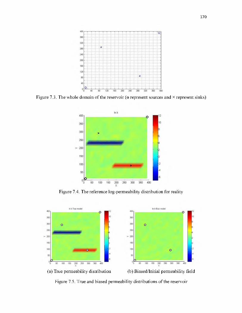
170

Figure 7.3. The whole domain of the reservoir (o represent sources and x represent sinks)

Figure 7.4. The reference log-permeability distribution for reality

(a) True permeability distribution (b) Biased/Initial permeability field

Figure 7.5. True and biased permeability distributions of the reservoir

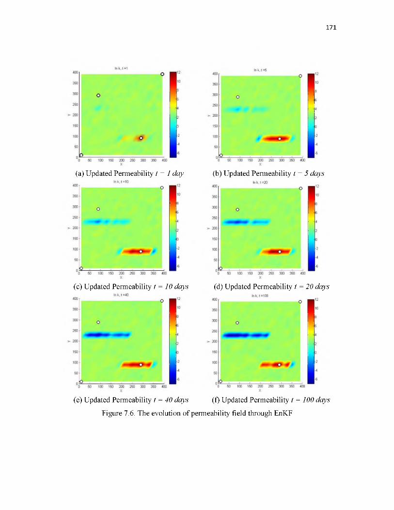
171

(a) Updated Permeability t = 1 day (b) Updated Permeability t = 5 days

(c) Updated Permeability t = 10 days (d) Updated Permeability t = 20 days

(e) Updated Permeability t = 40 days (f) Updated Permeability t = 100 days

Figure 7.6. The evolution of permeability field through EnKF

172

a

15

10

5

0I

5

0

-5

-10

(a) locate at open fracture (b) locate at open fracture12 I '

10

j ^

In k

CO

6

450

Time(c) locate at sealed fracture

100

50Time

50 Time

(d) Internal point

50Time

100 0

Figure 7.7. Permeability changing with time

100

2.9

V ______________:

2.8

2.7

2.6100

173

Figure 7.8. True, biased, measurement, and estimate output. (a) and (d) the bottom hole pressure of injection well 1 and well 4; (b) and (c) the production rate of well 2 and well

3; (e) and (f) the pressure of monitoring wells

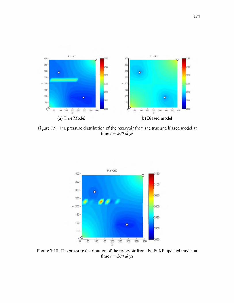
174

P. t =200 P, t =200

(a) True Model (b) Biased model

Figure 7.9. The pressure distribution of the reservoir from the true and biased model attime t = 200 days

Figure 7.10. The pressure distribution of the reservoir from the EnKF updated model attime t = 200 days

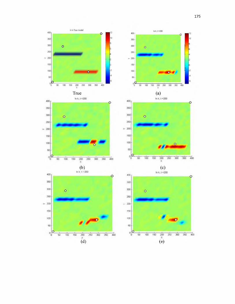
175

400

300

260

200

150

too

50

0

(b) h k. t *200

r 400 r ___________ ^V o[ yyi L

o 300 o■ _

[ y 200 [

I 150

•, / • 1

,0° § .O

r a

h __ Ol o ............................................0 50 100 150 200 250 300 350 400

X

(d)

0 50 tOO 150 200 250 300 350 400

(e)

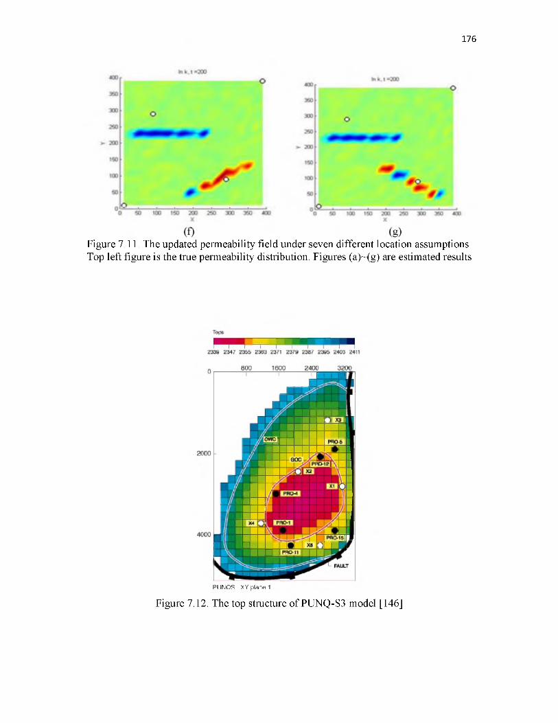
176

Figure 7.11. The updated permeability field under seven different location assumptions. Top left figure is the true permeability distribution. Figures (a)~(g) are estimated results

PUNQS XY plane 1

Figure 7.12. The top structure of PUNQ-S3 model [146]

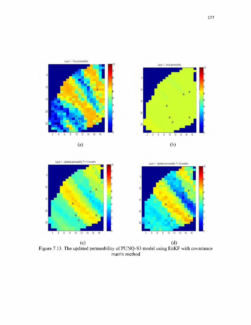
177

(b)

(c) (d)Figure 7.13. The updated permeability of PUNQ-S3 model using EnKF with covariance

matrix method

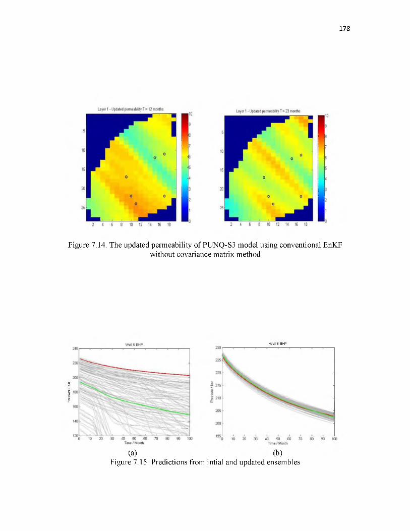
Pres

sure

/

bar

178

Figure 7.14. The updated permeability of PUNQ-S3 model using conventional EnKFwithout covariance matrix method

W e ll 5 BH P

(a) (b)Figure 7.15. Predictions from intial and updated ensembles

C H A PT E R 8

CONCLUSIONS AND FUTURE WORK

In this chapter, the work done in this research is summarized, and some future work is

recommended.

8.1 Summary of Research Work

This research contains three major parts: 1. Geomechanics modeling. Hydraulic

fractures’ opening, propagating, and interacting mechanically with other HFs and NFs are

investigated through numerical simulations; 2. Flow simulation. The nonplanar, more

realistic hydraulic fracture geometry is applied into the flow simulator to predict the

production performance; 3. Data assimilation. Those uncertain geological reservoir

properties are calibrated by integrating the production data and using the inversion

algorithm. Some of the important accomplishments and findings of this research are

summarized as the following.

1. Further development of hydraulic fracture simulator. This simulator based on dual­

lattice discrete element method is a fully coupled geomechanics and flow simulator.

The mechanics of fracture propagations and interactions are calculated based on

the DEM particle network, and the fluid flow is explicitly calculated based on

conjugate flow lattice. The introduction o f a dual-lattice system greatly

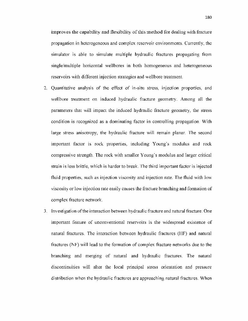
im proves the capability and flexibility o f this m ethod for dealing with fracture

propagation in heterogeneous and complex reservoir environments. Currently, the

simulator is able to simulate multiple hydraulic fractures propagating from

single/multiple horizontal wellbores in both homogeneous and heterogeneous

reservoirs with different injection strategies and wellbore treatment.

2. Quantitative analysis of the effect of in-situ stress, injection properties, and

wellbore treatment on induced hydraulic fracture geometry. Among all the

parameters that will impact the induced hydraulic fracture geometry, the stress

condition is recognized as a dominating factor in controlling propagation. With

large stress anisotropy, the hydraulic fracture will remain planar. The second

important factor is rock properties, including Young’s modulus and rock

compressive strength. The rock with smaller Young’s modulus and larger critical

strain is less brittle, which is harder to break. The third important factor is injected

fluid properties, such as injection viscosity and injection rate. The fluid with low

viscosity or low injection rate easily causes the fracture branching and formation of

complex fracture network.

3. Investigation of the interaction between hydraulic fracture and natural fracture. One

important feature of unconventional reservoirs is the widespread existence of

natural fractures. The interaction between hydraulic fractures (HF) and natural

fractures (NF) will lead to the formation of complex fracture networks due to the

branching and merging of natural and hydraulic fractures. The natural

discontinuities will alter the local principal stress orientation and pressure

distribution when the hydraulic fractures are approaching natural fractures. When

180

181

HFs are intercepting single or multiple NFs, complex mechanisms such as direct

crossing, arresting, dilating, and branching can be accurately simulated based on

the proposed simulator. The parameters that affect the HF/NF interaction include

in-situ stress anisotropy, natural fracture orientation, cohesion, and permeability

and injection fluid properties. The natural fractures will be more easily reactivated

with small stress difference and low injection viscosity/rate.

4. Integration of the realistic hydraulic fracture geometry with flow simulator. After

mapping the nonplanar fracture into a regular mesh grid, reservoir volume accessed

by the complex fracture is different from the reservoir volume accessed by

simplified planar fracture models, which are dependent on the complexity of the

fracture morphology. The assumption of an orthogonal planar fracture will lead to

deviations of production performance.

5. Development of covariance matrix method based on EnKF algorithm. The novel

proposed model uncertainty covariance matrix method enables the direct

incorporation of the reservoir spatial information into the conventional EnKF

algorithm. Both the fracture properties (orientation and permeability) and formation

heterogeneity can be accurately captured.

8.2 Recommendations of Future Work

The DEM simulator is a general-purpose research simulator with greater capability and

flexibility. The following are the recommendations for possible further work:

1. Development of three dimensional DEM simulator. The model proposed in this

thesis is still a two-dimensional model with the assumption of plane strain. In the

reality, the unconventional reservoir is always three-dimensional with certain

depth. Ignoring the fracture propagation in other dimension is not accurate.

2. Nonisotropic geomechanical parameters. The mechanical properties used in this

DEM simulator are assumed to be isotropic. However, lots of geological data reveal

that the rock is anisotropic, the Young’s modulus difference in horizontal and

vertical directions are especially large. It is worthwhile to implement this

functionality in the model.

3. Proppant transport. The induced hydraulic fracture will be easily closed if there is

not proppant injected with the fracking fluid. The proppant’s transportation and

distribution determine the ultimate conductive path connecting the formation to the

wellbore. Therefore, modeling of proppant transport plays a substantial role in

unconventional reservoir stimulation.

4. Nonlinear constitutive relationship. In this DEM simulator, we assume the rock is

a linear elastic formation. However, the rock or soil behaves nonlinearly in some

cases, especially when rock deforms or breaks. The computational efficiency and

convergence may be a potential problem if a nonlinear constitutive law is used.

5. Calibrate the model using the microseimic data based on Ensemble Kalman Filter.

Since the oil and gas reservoirs are far below the surface, it is very hard or nearly

impossible to directly measure either detailed properties or the generated fracture

geometry. Also, the parameters used in the model have large uncertainties. In order

to provide feasible guidance in optimizing the stimulation strategy, the model has

to calibrate and match the performance of the reservoirs. The microseismic events

are believed to carry information about underlying fluid flow and geomechanics.

182

Therefore the model will be more reliable by using the microseismic data to

calibrate the model.

6. Other numerical methods combined with DEM simulator. Each numerical method

has its own advantages and disadvantages. There is no perfect method for solving

different problems. The continuum methods are more suitable for simulating rock

mass with no fractures. And the discrete method is more suitable for moderately

fractured rock mass. By combining different continuum-discrete models, some

disadvantages in one type may be avoided.

183

REFERENCES

[1] U. S. Energy Information Administration, “Annual Energy Outlook.”, 2015.

[2] K. Wu, “Numerical Modeling of Complex Hydraulic Fracture Development in Unconventional Reservoirs,” Ph.D. dissertation, Dept. Pet. Geosci. Eng., The Univ. of Texas at Austin, Austin, TX, 2014.

[3] J. Adachi, E. Siebrits, A. Peirce, and J. Desroches, “Computer simulation of hydraulic fractures,” Int. J. RockMech. Mining Sci., vol. 44, pp. 739-757, 2007.

[4] J. J. Grebe and M. Stoesser, “Increasing Crude Production 20,000,000 Barrels from Established Fields,” World Pet., vol. 6, no. 8, pp. 473-482, 1935.

[5] P. Valko and M. J. Economides, Hydraulic Fracture Mechanics. New Jersey: Wiley, 1996.

[6] E. L. Hagstrom and J. M. Adams, “Hydraulic Fracturing: Identifying and Managing the Risks,” Environ. Claims J., vol. 24, no. 2, pp. 93-115, 2012.

[7] T. H. Yang, L. G. Tham, C. A. Tang, Z. Z. Liang, and Y. Tsui, “Influence of Heterogeneity of Mechanical Properties on Hydraulic Fracturing in Permeable Rocks,” Rock Mech. Rock Eng., vol. 37, no. 4, pp. 251-275, 2004.

[8] N. R. Warpinski, M. J. Mayerhofer, M. C. Vincent, C. L. Cipolla, and E. P. Lolon, “ Stimulating Unconventional Reservoirs: Maximizing Network Growth While Optimizing Fracture Conductivity,” J. Can. Pet. Technol., vol. 48, no. 10, pp. 39­51, 2009.

[9] N. Zhao, J. McLennan, and M. Deo, “Morphology and Growth of Fractures in Unconventional Reservoirs,” in Canadian Unconventional Resources Conference,15-17 November, Calgary, 2011, pp. 1-14.

[10] L. Jing, “A review of techniques, advances and outstanding issues in numerical modelling for rock mechanics and rock engineering,” Int. J. Rock Mech. Min. Sci., vol. 40, no. 4, pp. 283-353, 2003.

[11] R. W. Clough, “The finite element method in plane stress analysis,” in ASCE 2nd Conference on Electronic Computation, September 8-9, 1960.

185

121 B. Patzak and M. Jirasek, “Adaptive Resolution of Localized Damage in Quasi- brittle Materials,” J. Eng. Mech., vol. 130, pp. 720-732, 2004.

131 M. A. Jaswon, “Integral Equation Methods in Potential Theory. I,” in Proceedings Royal Society London A, 1963, pp. 23-32.

141 G. T. Symm, “Integral Equation Methods in Potential Theory. II,” in Proceedings Royal Society London A, 1963, pp. 33-46.

151 T. A. Cruse, “Two-dimensional BIE fracture mechanics analysis,” Appl. Math. Model., vol. 2, no. 4, pp. 287-293, 1978.

161 Q. Li, H. Xing, J. Liu, and X. Liu, “Review article A review on hydraulic fracturing of unconventional reservoir,” Petroleum, vol. 1, pp. 8-15, 2015.

171 S. A. Khristianovic and Y. P. Zheltov, “Formation of Vertical Fractures by means of Highly Viscous Liquid,” in 4th World Petroleum Congress, 1955, vol. 5.

181 J. Geertsma and F. d. Klerk, “A Rapid Method of Predicting Width and Extent of Hydraulically Induced Fractures,” J. Pet. Technol., vol. 21, no. 12, pp. 1571-1581,1969.

191 T. K. Perkins and L. R. Kern, “Widths of Hydraulic Fractures,” J. Pet. Technol., vol. 13, no. 09, pp. 937-949, Apr. 1961.

201 R. P. Nordgren, “Propagation of a Vertical Hydraulic Fracture,” Soc. Pet. Eng. J., vol. 12, no. 04, pp. 306-314, 1972.

211 I. N. Sneddon, Fourier transforms. New York: McGraw-Hill, 1951.

221 A. A. Daneshy, “On the Design of Vertical ‘ Hydraulic Fractures,” J. Pet. Technol., vol. 25, no. 01, pp. 83-97, 1973.

231 D. A. Spence and P. Sharp, “Self-Similar Solutions for Elastohydrodynamic Cavity Flow,” in Proceedings Royal Society London A, 1985, pp. 289-313.

241 E. R. Simonson, A. S. Abou-Sayed, and R. J. Clifton, “Containment of Massive Hydraulic Fractures,” Soc. Pet. Eng. J., vol. 18, no. 01, pp. 27-32, 1978.

251 S. H. Advani and J. K. Lee, “Finite Element Model Simulations Associated With Hydraulic Fracturing,” Soc. Pet. Eng. J., vol. 22, no. 02, pp. 209-218, 1982.

261 R. J. Clifton and A. S. Abou-Sayed, “a Variational Approach To the Prediction of the Three-Dimensional Geometry of,” SPE/DOELow Perm GasReserv. Symp. 27­29 May, Denver, pp. 457-465, 1981.

186

[27] A. Settari and M. P. Cleary, “Three-Dimensional Simulation of Hydraulic Fracturing,” J. Pet. Technol., vol. 36, no. 07, pp. 1177-1190, 1984.

[28] H. A. M. Van Eekelen, “Hydraulic Fracture Geometry : Fracture Containment in Layered Formations,” Soc. Pet. Eng. J., vol. 22, no. 03, pp. 341-349, 1982.

[29] R. L. Fung, S. Vilayakumar, and D. Cormack, “Calculation of Vertical Fracture Containment in Layered Formations,” SPE Form. Eval., vol. 2, no. 04, pp. 518­522, 1987.

[30] M. P. Cleary, M. Kavvadas, and K. Y. Lam, “Development of a Fully Three­Dimensional Simulator for Analysis and Design of Hydraulic Fracturing,” in SPE/DOE Low Permeability Gas Reservoirs Symposium, 14-16 March, Denver, Colorado, 1983, pp. 271-282.

[31] X. Weng, “Modeling of complex hydraulic fractures in naturally fractured formation,” J. Unconv. Oil Gas Resour., vol. 9, pp. 114-135, Sep. 2015.

[32] S. L. Crouch, “Solution of plane elasticity problems by the displacement discontinuity method,” Int. J. Numer. Methods Eng., vol. 10, no. 2, 1976.

[33] J. E. Olson, “Predicting fracture swarms — the influence of subcritical crack growth and the crack-tip process zone on joint spacing in rock,” in Geological Society, London, Special Publications, 231:73-88.

[34] F. Erdogan and G. C. Sih, “On the Crack Extension in Plates under Loading and Transverse Shear,” J. Fluids Eng., vol. 85, no. 4, pp. 519-527, 1963.

[35] G. C. Sih, “Strain energy density factor applied to mixed mode problems,” Int. J. Fract., vol. 10, no. 3, pp. 305-321, 1974.

[36] R. J. Nuismer, “An energy release rate criteria for mixed mode fracture,” Int. J. Fract., vol. 11, no. 2, pp. 245-250, 1975.

[37] C. Y. Dong and C. J. De Pater, “Numerical implementation of displacement discontinuity method and its application in hydraulic fracturing,” Comput. Methods Appl. Mech. Eng., vol. 191, no. 8-10, pp. 745-760, 2001.

[38] J. E. Olson, “Multi-fracture propagation m odeling: Applications to hydraulic fracturing in shales and tight gas sands,” in The 42nd U.S. Rock Mechanics Symposium (USRMS), 29 June-2 July, San Francisco, California, 2008.

[39] Y. Cheng, “Boundary Element Analysis of the Stress Distribution around Multiple Fractures : Implications for the Spacing of Perforation Clusters of Hydraulically Fractured Horizontal Wells,” in SPE Eastern Regional Meeting, 23-25 September, Charleston, West Virginia, USA, 2009.

187

[40] J. E. Olson and K. Wu, “Sequential versus Simultaneous Multi-zone Fracturing in Horizontal Wells : Insights from a Non-planar , Multi-frac Numerical Model,” in Hydraulic Fracturing Technology Conference, Woodlands, Texas, USA, 6-8 February, 2012, no. 2011.

[41] K. Wu and J. E. Olson, “Study of Multiple Fracture Interaction Based on An Efficient Three-Dimensional Displacement Discontinuity Method,” in 49th US Rock Mechanics / Geomechanics Symposium held in San Francisco, CA, USA, 28 June- 1 July, 2015.

[42] K. Wu and J. E. Olson, “Investigation of the Impact of Fracture Spacing and Fluid Properties for Interfering Simultaneously or Sequentially Generated Hydraulic Fractures,” in Hydraulic Fracturing Technology Conference, Woodlands, Texas, USA, 6-8 February, 2013, no. February.

[43] V. Sesetty and A. Ghassemi, “Numerical Simulation of Sequential and Simultaneous Hydraulic Fracturing,” in Effective and Sustainable Hydraulic Fracturing,DOI: 10.5772/56309, vol. d, 2013.

[44] H. Jo, “Optimizing Fracture Spacing to Induce Complex Fractures in a Hydraulically Fractured Horizontal Wellbore,” in Americas Unconventional Resources Conference, Pittsburgh, Pennsylvania, USA, 5-7 June, 2012.

[45] A. P. Bunger, X. Zhang, and R. G. Jeffrey, “Parameters Effecting the Interaction among Closely Spaced Hydraulic Fractures,” in Hydraulic Fracturing Technology Conference, Woodlands, Texas, USA, 24-26 January, 2011.

[46] J. Desroches, E. Detournay, B. Lenoach, P. Papanastasiou, J. R. A. Pearson, M. Thiercelin, and A. Cheng, “The Crack Tip Region in Hydraulic Fracturing,” in Proceedings Royal Society London A, 1994, pp. 39-48.

[47] B. Lenoach, “The Crack Tip Solution For Hydraulic Fracturing in a Permeable Solid,” J. Mech. Phys. Solids, vol. 43, no. 7, pp. 1025-1043, 1995.

[48] A. Dahi-Taleghani, “Analysis of hydraulic fracture propagation in fractured reservoirs: an improved model for the interaction between induced and natural fractures,” Ph.D. dissertation, Dept. Pet. Geosci. Eng., The Univ. of Texas at Austin, Austin, TX, 2009.

[49] S. Wong, M. Geilikman, S. I. Exploration, and G. Xu, “Interaction of Multiple Hydraulic Fractures in Horizontal Wells,” in Middle East Unconventional Gas Conference and Exhibition, Muscat, Oman, 28-30 January, 2013.

[50] N. P. Roussel and M. M. Sharma, “Optimizing Fracture Spacing and Sequencing in Horizontal-Well Fracturing,” SPE Prod. Oper., vol. 26, no. 02, pp. 173-184, 2011.

188

[51] N. P. Roussel and M. M. Sharma, “Strategies to Minimize Frac Spacing and Stimulate Natural Fractures in Horizontal Completions,” in Annual Technical Conference and Exhibition held in Denver, Colorado, USA, 30 October-2 November, 2011.

[52] K. Yamamoto, T. Shimamoto, and S. Sukemura, “Multiple Fracture Propagation Model for a Three-Dimensional Hydraulic Fracturing Simulator,” Int. J. Geomech., vol. 4, no. 1, pp. 46-57, 2004.

[53] S. T. Castonguay, M. E. Mear, R. H. Dean, and J. H. Schmidt, “Predictions of the Growth of Multiple Interacting Hydraulic Fractures in Three Dimensions,” in SPE Annual Technical Conference and Exhibition, 30 September-2 October, New Orleans, Louisiana, USA, 2013.

[54] D. H. Shin and M. M. Sharma, “Factors Controlling the Simultaneous Propagation of Multiple Competing Fractures in a Horizontal Well,” in Hydraulic Fracturing Technology Conference, Woodlands, Texas, USA, 4-6 February, 2014, no. 2009.

[55] B. J. Carter, P. A. Wawrzynek, and A. R. Ingraffea, “Automated 3D Crack Growth Simulation,” Int. J. Numer. Methods Eng., vol. 47, pp. 229-253, 2000.

[56] P. O. Bouchard, F. Bay, Y. Chastel, and I. Tovena, “Crack propagation modelling using an advanced remeshing technique,” Comput. Methods Appl. Mech. Eng., vol. 189, no. 3, pp. 723-742, 2000.

[57] N. Moes, J. Dolbow, and T. Belytschko, “A Finite Element Method for Crack Growth Without Remeshing,” Int. J. Numer. Methods Eng., vol. 46, no. 1, pp. 131-150, 1999.

[58] T. Strouboulis, I. Babuska, and K. Copps, “The design and analysis of the Generalized Finite Element Method,” Comput. Methods Appl. Mech. Eng., vol. 181, no. 1-3, pp. 43-69, 2000.

[59] T. Belytschko and T. Black, “Elastic Crack Growth in Finite Elements With Minimal Remeshing,” Int. J. Numer. Methods Eng., vol. 45, no. 5, pp. 601-620, 1999.

[60] C. Daux, N. Moes, J. Dolbow, N. Sukumar, and T. Belytschko, “Arbitrary branched and intersecting cracks with the extended finite element method,” Int. J. Numer. Methods Eng., vol. 48, no. 12, pp. 1741-1760, 2000.

[61] N. Sukumar, N. Moes, B. Moran, and T. Belytschko, “Extended finite element method for three-dimensional crack modelling,” Int. J. Numer. Methods Eng., vol. 48, no. 11, pp. 1549-1570, 2000.

[62] N. Moes and T. Belytschko, “Extended finite element method for cohesive crack

189

growth,” Eng. Fract. Mech., vol. 69, no. 7, pp. 813-833, 2002.

[631 A. Dahi-Taleghani and J. Olson, “Numerical Modeling of Multistranded- Hydraulic-Fracture Propagation: Accounting for the Interaction Between Induced and Natural Fractures,” SPE J., vol. 16, no. September, pp. 575-581, 2011.

[641 J. Rethore, A. Gravouil, and A. Combescure, “An energy-conserving scheme for dynamic crack growth using the extended finite element method,” Int. J. Numer. Methods Eng., vol. 63, no. 5, pp. 631-659, 2005.

[651 J. Song, P. M. A. Areias, and T. Belytschko, “A method for dynamic crack and shear band propagation with phantom nodes,” Int. J. Numer. Methods Eng., vol. 67, no. 6, pp. 868-893, 2006.

[661 J. L. Asferg, P. N. Poulsen, and L. O. Nielsen, “A consistent partly cracked XFEM element for cohesive crack growth,” Int. J. Numer. Methods Eng., vol. 75, no. 4, pp. 464-485, 2007.

[671 A. Simone, C. A. Duarte, and E. Van der Giessen, “A Generalized Finite Element Method for polycrystals with discontinuous grain boundaries,” Int. J. Numer. Methods Eng., vol. 67, pp. 1122-1145, 2006.

[681 P. A. Cundall and O. D. . Strack, “A discrete numerical model for granular assemblies,” Geotechnique, vol. 29, no. 1, pp. 47-65, 1979.

[691 D. O. Potyondy, P. A. Cundall, and C. A. Lee, “Modelling rock using bonded assemblies of circular particles,” in 2nd North American Rock Mechanics Symposium, 19-21 June, Montreal, Quebec, Canada, 1996, pp. 1937-1944.

[701 D. O. Potyondy and P. a. Cundall, “A bonded-particle model for rock,” Int. J. Rock Mech. Min. Sci., vol. 41, no. 8, pp. 1329-1364, Dec. 2004.

[711 G. A. D ’Addetta and F. K. Ramm, “On the application of a discrete model to the fracture process of cohesive granular materials,” Granul. Matter, vol. 4, no. 2, pp. 77-90, 2002.

[721 F. Zhang, B. Damjanac, and H. Huang, “Coupled discrete element modeling of fluid injection into dense granular media,” J. Geophys. Res. Solid Earth, vol. 118, no. 6, pp. 2703-2722, 2013.

[731 P. A. Cundall, “A computer model for simulating progressive large scale movements in blocky rock systems,” in Proceedings o f the international symposium on rock fracture, Nancy, pp. 129-136.

[741 M. Bai, S. Green, L. Casas, and J. Miskimins, “3-D Simulation of Large Scale Laboratory Hydraulic Fracturing Tests,” in Golden Rocks 2006, The 41st U.S.

190

Symposium on Rock Mechanics (USRMS), 17-21 June, Golden, Colorado, 2006.

[75] B. C. Haimson, “Large Scale Laboratory Testing of Hydraulic Fracturing,” Geophys. Res. Lett., vol. 8, no. 7, pp. 715-718, 1981.

[76] R. L. J. Johnson and C. W. Greenstreet, “Managing Uncertainty Related to Hydraulic Fracturing Modeling in Complex Stress Environments with Pressure- Dependent Leakoff,” in SPE Annual Technical Conference and Exhibition, 5-8 October, Denver, Colorado, 2003.

[77] M. P. Scott, R. L. Johnson, A. Datey, C. B. Vandenborn, and R. A. Woodroof, “Evaluating Hydraulic Fracture Geometry from Sonic Anisotropy and Radioactive Tracer Logs,” in SPE Asia Pacific Oil and Gas Conference and Exhibition, 18-20 October, Brisbane, Queensland, Australia, 2010.

[78] H. Huang and E. Mattson, “Physics-based Modeling of Hydraulic Fracture Propagation And Permeability Evolution of Fracture Network In Shale Gas Formation,” in 2014 ARMA 48th US Rock Mechanics/Geomechanics Symposium,Minneapolis, MN, 1-4 June 2014, 2014.

[79] Y. Yang, “Finite-Element Multiphase Flow Simulation,” Ph.D. dissertation, Dept. Chem. Eng., The Univ. of Utah, Salt Lake City, UT, 2003.

[80] Q. M. Li, “Strain energy density failure criterion,” Int. J. Solids Struct., vol. 38, pp. 6997-7013, 2001.

[81] L. Jing, “A review of techniques, advances and outstanding issues in numerical modelling for rock mechanics and rock engineering,” Int. J. RockMech. Min. Sci., vol. 40, no. 3, pp. 283-353, 2003.

[82] K. A. Owens, S. A. Andersen, and M. J. Economides, “Fracturing Pressures for Horizontal Wells,” in SPE Annual Technical Conference and Exhibition, 4-7 October, Washington, D.C., 1992.

[83] L. Weijers and C. J. De Pater, “Fracture Reorientation in Model Tests,” in SPE Formation Damage Control Symposium, 26-27 February, Lafayette, Louisiana, 1992.

[84] J. E. Olson, “Fracturing from Highly Deviated and Horizontal Wells : Numerical Analysis of Non- planar Fracture Propagation,” in Low Permeability Reservoirs Symposium, 19-22 March, Denver, Colorado, 1995, pp. 275-287.

[85] V. F. Rodrigues, L. F. Neumann, D. S. Torres, C. Guimaraes, and R. S. Torres, “Horizontal Well Completion and Stimulation Techniques — A Review With Emphasis on Low-Permeability Carbonates,” in Latin American & Caribbean Petroleum Engineering Conference, 15-18 April, Buenos Aires, Argentina, 2007.

191

[86] M. Y. Soliman, L. E. East, and D. L. Adams, “Geomechanics Aspects of Multiple Fracturing of Horizontal and Vertical Wells,” SPEDrill. Complet., vol. 23, no. 03, pp. 217-228, 2008.

[87] J. P. Vermylen, “Geomechanical Studies of the Barnett Shale, Texas, USA,” Ph.D. dissertation, Dept. Geophysics , Stanford University, Standord, CA,2011.

[88] W. El Rabaa, “Experimental Study of Hydraulic Fracture Geometry Initiated From Horizontal Wells,” in SPE Annual Technical Conference and Exhibition, 8-11 October, San Antonio, Texas, 1989.

[89] H. H. Abass, M. Y. Soliman, A. M. Al-Tahini, J. B. Surjaatmadja, D. L. Meadows, and L. Sierra, “Oriented Fracturing : A New Technique to Hydraulically Fracture Openhole Horizontal Well,” in SPE Annual Technical Conference and Exhibition, 4-7 October, New Orleans, Louisiana, 2009.

[90] G. E. King, “Thirty years of gas-shale fracturing: What have we learned?,” in SPE Annual Technical Conference and Exhibition, 19-22 September, Florence, Italy, 2010.

[91] A. Kissinger, R. Helmig, A. Ebigbo, H. Class, T. Lange, M. Sauter, M. Heitfeld, J. Klunker, and W. Jahnke, “Hydraulic fracturing in unconventional gas reservoirs : risks in the geological system , part 2,” Environ. Earth Sci., vol. 70, no. 8, pp. 3855-3873, 2013.

[92] J. McLennan, D. Tran, N. Zhao, S. Thakur, M. Deo, I. Gil, and B. Damjanac, “Modeling Fluid Invasion and Hydraulic Fracture Propagation in Naturally Fractured R ock : A Three-Dimensional Approach,” in 2010 SPE International Symposium and Exhibition on Formation Damage Control, Lafayette, Louisiana, USA, 10-12 February., 2010, pp. 1-13.

[93] N. R. Warpinski and L. W. Teufel, “Influence of Geologic Discontinuities on Hydraulic Fracture Propagation,” J. Pet. Technol., vol. 39, 1987.

[94] L. Teufel and J. Clark, “Hydraulic Fracture Propagation in Layered Rock: Experimental Studies of Fracture Containment,” Soc. Pet. Eng. J., vol. 24, no. February, pp. 19-32, 1984.

[95] T. Blanton, “An Experimental Study of Interaction Between Hydraulically Induced and Pre-Existing Fractures,” in Proceedings o f SPE Unconventional Gas Recovery Symposium, 1982, pp. 559-571.

[96] M. Fisher and C. Wright, “Integrating fracture mapping technologies to optimize stimulations in the barnett shale,” in SPE Annual Technical Conference and Exhibition, 29 September-2 October 2002, San Antonio, Texas, 2002, pp. 1-7.

192

[97] C. E. Renshaw and D. D. Pollard, “An experimentally verified criterion for propagation across unbounded frictional interfaces in brittle, linear elastic materials,” Int. J. Rock Mech. Min. Sci. Geomech. Abstr., vol. 32, no. 3, pp. 237­249, 1995.

[98] H. Gu and X. Weng, “Criterion for Fractures Crossing Frictional Interfaces at Non-orthogonal Angles,” 44th US Rock Mech. Symp. 5th U.S.-Canada Rock Mech. Symp. 27-30 June, Salt Lake City, pp. 1-6, 2010.

[99] D. Chuprakov, O. Melchaeva, and R. Prioul, “Injection-Sensitive Mechanics of Hydraulic Fracture Interaction with Discontinuities,” in 47th U.S. Rock Mechanics/Geomechanics Symposium, 23-26 June, San Francisco, California, 2013.

[100] J. E. Olson and A. D. Taleghani, “Modeling simultaneous growth of multiple hydraulic fractures and their interaction with natural fractures,” in SPE 119739 Hydraulic Fracturing Technology Conference, Woodlands, Texas, USA, 19-21 January, 2009.

[101] V. Sessety and A. Ghassemi, “Simulation of Hydraulic Fractures and their Interactions with Natural Fractures,” in 46th U.S. Rock Mechanics/Geomechanics Symposium, 24-27 June, Chicago, Illinois, 2012.

[102] O. Kresse, X. Weng, D. Chuprakov, R. Prioul, and C. Cohen, “Effect of Flow Rate and Viscosity on Complex Fracture Development in UFM Model,” in Effective and Sustainable Hydraulic Fracturing, DOI: 10.5772/56406, 2013.

[103] K. Wu and J. E. Olson, “Mechanics Analysis of Interaction Between Hydraulic and Natural Fractures in Shale Reservoirs,” in Proceedings o f the 2nd Unconventional Resources Technology Conference, 2014.

[104] J. Huang, R. Safari, K. Burns, I. Geldmacher, U. Mutlu, M. McClure, and S. Jackson, “Natural-Hydraulic Fracture Interaction: Microseismic Observations and Geomechanical Predictions,” in Proceedings o f the 2nd Unconventional Resources Technology Conference, 2014, pp. 1-22.

[105] J. Huang, X. Ma, R. Safari, U. Mutlu, and M. Mcclure, “Hydraulic Fracture Design Optimization for Infill Wells : An Integrated Geomechanics Workflow,” in The 49th US Rock Mechanics/Geomechanics Symposium held in San Francisco, CA, USA, 28 June-1 July, 2015.

[106] J. F. W. Gale, R. M. Reed, and J. Holder, “Natural fractures in the Barnett Shale and their importance for hydraulic fracture treatments,” in AAPG Bulletin, 2007, vol. 91, no. 4, pp. 603-622.

[107] F. Zhang, N. Nagel, and F. Sheibani, “Evaluation of Hydraulic Fractures Crossing

193

Natural Fractures at High Angles Using a Hybrid Discrete-Continuum Model,” in 48th US Rock Mechanics/Geomechanics Symposium held in Minneapolis, MN, USA, 1-4 June, 2014.

[1081 W. Yu, S. Huang, K. Wu, K. Sepehrnoori, and W. Zhou, “Development of a Semi- Analytical Model for Simulation of Gas Production in Shale Gas Reservoirs,” in SPE/AAPG/SEG Unconventional Resources Technology Conference, 25-27 August , Denver, Colorado, USA, 2014.

[1091 H. Moradkhani, S. Sorooshian, H. V. Gupta, and P. R. Houser, “Dual state- parameter estimation of hydrological models using ensemble Kalman filter,” Adv. Water Resour., vol. 28, no. 2, pp. 135-147, Feb. 2005.

[1101 X. Yang, K. Shi, and K. Xing, “Joint parameter and state estimation based on particle filtering and stochastic approximation,” Comput. Intell. ..., pp. 0-3, 2006.

[1111 A. H. Jazwinski, Stochastic Processes and Filtering Theory. Academic Press,1970.

[1121 I. Navon, “Practical and theoretical aspects of adjoint parameter estimation and identifiability in meteorology and oceanography,” Dyn. Atmos. Ocean., 1998.

[1131 M. Kudisch, “Off-line parameter and state estimation for power electronic circuits,” Power Electron. 1988.

[1141 L. Ljung, System Identification Theory for the User, 2nd ed. New Jersey: Prentice Hall PTR, 1999.

[1151 G. M. Siouris, An Engineering Approach to Optimal Control and Estimation Theory. New Jersey: Wiley-Interscience, 1996.

[1161 Z. Zhang, “Parameter estimation techniques: A tutorial with application to conic fitting,” Image Vis. Comput., 1997.

[1171 J. Aldrich, “Doing least squares: Perspectives from Gauss and Yule,” Int. Stat. Rev., no. 1967, 1998.

[1181 J. O. Berger, Statistical Decision Theory and Bayesian Analysis, 2nd ed. New York: Springer, 1985.

[1191 R. . Fisher, “On the Mathematical Foundations of Theoretical Statistics,” Philos. Trans. R. Soc. A, vol. 222, pp. 309-368, 1922.

[1201 R. . Fisher, “Theory of Statistical Estimation,” Math. Proc. Cambridge Philos. Soc., vol. 22, no. 05, pp. 700-725, 1925.

194

[121] L. Le Cam, “Maximum likelihood: an introduction,” Stat. Rev. Int. Stat., 1990.

[122] D. S. Oliver, A. C. Reynolds, and N. Liu, Inverse Theory for Petroleum Reservoir Characterization and History Matching. Cambridge: Cambridge University Press, 2008.

[123] R. Kalman, “A new approach to linear filtering and prediction problems,” J. basic Eng., vol. 82, no. Series D, pp. 35-45, 1960.

[124] D. Simon, Optimal State Estimation: Kalman, H infinity, and Nonlinear Approaches. New Jersey: Wiley-Interscience, 2006.

[125] G. Welch and G. Bishop, “An Introduction to the Kalman Filter,” Dept. Comp. Sci., Univ. North Carolina at Chapel Hill, Chaple Hill, NC, Sci. Rep. July 2001.

[126] G. Evensen, “Sequential Data Assimilation With a Nonlinear Quasi- Geostrophic Model Using Monte Carlo Methods To Forecast Error Statistics,” J. Geophys. Res. Ocean., vol. 99, no. c5, pp. 10143-10162, 1994.

[127] G. N^vdal, T. Mannseth, and E. Vefring, “Near-well reservoir monitoring through ensemble Kalman filter,” Pap. SPE, no. 1, pp. 1-9, 2002.

[128] G. Evensen, “The Ensemble Kalman Filter: theoretical formulation and practical implementation,” OceanDyn., vol. 53, no. 4, pp. 343-367, Nov. 2003.

[129] S. Aanonsen, G. Naevdal, D. S. Oliver, A. C. Reynolds, and B. Valles, “The Ensemble Kalman Filter in Reservoir Engineering-a Review,” SPE J., pp. 393­412, 2009.

[130] A. Mesbah, A. E. M. Huesman, H. J. M. Kramer, and P. M. J. Van den Hof, “A comparison of nonlinear observers for output feedback model-based control of seeded batch crystallization processes,” J. Process Control, vol. 21, no. 4, pp. 652­666, Apr. 2011.

[131] C. Rao, J. Rawlings, and J. Lee, “Constrained linear state estimation— a moving horizon approach,” Automatica, vol. 37, pp. 1619-1628, 2001.

[132] E. Haseltine and J. Rawlings, “Critical evaluation of extended Kalman filtering and moving-horizon estimation,” Ind. Eng. Chem., vol. 44, no. 8, pp. 2451-2460, Apr. 2005.

[133] C. V. Rao, J. B. Rawlings, and D. Q. Mayne, “Constrained state estimation for nonlinear discrete-time systems: stability and moving horizon approximations,” IEEE Trans. Automat. Contr., vol. 48, no. 2, pp. 246-258, Feb. 2003.

[134] A. G. Qureshi, “Constrained Kalman filtering for image restoration,” Acoust.

195

Speech, Signal Process. 1989. pp. 1405-1408, 1989.

[135] J. De Geeter, “A smoothly constrained Kalman filter,” Pattern Anal., vol. 19, no. 10, pp. 1171-1177, 1997.

[136] D. Simon, “Kalman filtering with state equality constraints,” IEEE Trans. Aerosp. Electron. Syst., vol. 38, no. 1, pp. 128-136, 2002.

[137] S. Ko and R. R. Bitmead, “State estimation for linear systems with state equality constraints,” Automatica, vol. 43, no. 8, pp. 1363-1368, Aug. 2007.

[138] N. Gupta and R. Hauser, “Kalman filtering with equality and inequality state constraints,” Oxford Univ. Comp. Lab., Oxford, U.K., Sci. Rep., Feb. 2008.

[139] H. A. Phale and D. S. Oliver, “Data Assimilation Using the Constrained Ensemble Kalman Filter,” SPE J., vol. 16, no. 2, pp. 331-342, 2011.

[140] D. Zupanski and M. Zupanski, “Model error estimation employing an ensemble data assimilation approach,” Mon. Weather Rev., no. 1994, pp. 1337-1354, 2006.

[141] G. Burgers, “Analysis scheme in the ensemble Kalman filter,” Mon. Weather, pp. 1719-1724, 1998.

[142] P. K. Kitanidis, Introduction to Geostatistics: applications in hydrogeology. Cambridge: Cambridge University Press, 1997.

[143] Imperial College London, "Standard Models PUNQ-S3 model". Internet: http://www3.imperial.ac.uk/earthscienceandengineering/research/perm/punq- s3model.” .