HYDRAULIC DEVELOPMENT OF A CENTRIFUGAL PUMP … · A CENTRIFUGAL PUMP IMPELLER USING THE AGILE...

TASK QUARTERLY 6 No 1 (2002), 79–100

HYDRAULIC DEVELOPMENT OFA CENTRIFUGAL PUMP IMPELLER

USING THE AGILE TURBOMACHINERYDESIGN SYSTEM

KRZYSZTOF DENUS1 AND COLIN OSBORNE2

1CTD Technology – Ing. Buro Denus,Stationstraße 37, Postfach 12, CH-8487 Zell, Switzerland

[email protected]

2Concepts NREC,217 Billing Farm Rd., White River Jct., VT 05001, USA

[email protected]

(Received 15 August 2001; revised manuscript received 28 December 2001)

Abstract: The impeller of an existing industrial pump (with both geometry and performanceknown) was analyzed and redesigned using an integrated, design/analysis, turbomachinery geometrymodeling and flow simulation system. The purpose of the redesign was to achieve improved impellerperformance (at the duty point). Fluid dynamics and geometry modeling parts of the design/analysissystem were systematically applied: a) to analyse the existing impeller (impeller A), which wasdesigned using conventional (routine in industry) hydraulic layout procedures, and b) to developa new impeller (impeller B), using a coupled, multilevel 1D-Q3D-3D for the design and optimization.This paper discusses the features and advantages of the integrated design system, in which the coupledCAD/CFD approach is fully implemented. The analysis results are presented for impellers A and B,with the latter demonstrating a predicted increased efficiency and smaller size. Comparisons of theCFD results for both impellers reveal internal flow features that explain the improved impeller Bperformance levels.

Keywords: impeller design, CFD analysis, turbomachinery design optimization, internal flowanalysis

NotationB – impeller channel width;BEP – best efficiency point;Beta – blade angle;E – impeller flow modeling parameter – the ratio between the secondary zone

area and the total area at the impeller outlet;H – developed head (pressure rise);Lax – axial length of the impeller channel;LE – impeller blade leading edge;

tq0106e7/79 26I2002 BOP s.c., http://www.bop.com.pl

80 K. Denus and C. Osborne

M – meridional distance;Q – flow rate;R – radius, impeller contour coordinate in the radial direction;S3x – local coordinate in the pitchwise direction;S3y – local coordinates in the spanwise direction;TE – impeller blade trailing edge;Z – impeller contour coordinate in the axial direction.

1. IntroductionThis paper discusses and presents the results of the application of the Agile

Engineering Design System©R [1], for the analysis and redesign of an exisiting industrialpump impeller. The subject impeller of this paper is from a high specific speedcentifugal pump stage which was designed by Sulzer Pumps Company, and was laterthe subject of a research program at the Swiss Federal Institute of Technology inZurich. The data which support the work described herein were derived from [2]and were used to reconstruct the key blading features of the tested impeller. In thispaper, this digitally reconstructed baseline impeller is referred to as impeller A. Thenew impeller, whose geometry was generated by the application of the Agile system,is referred to as impeller B, which could serve as a replacement for impeller A.

Within the redesign process, two steps were undertaken in order to improve thebaseline pump impeller A:

1. To analyze the performance of the baseline impeller A using the multilevelanalysis tools available within the Agile system, which includes 1D, Q3D, andfully 3D, Navier-Stokes solvers.

2. To redesign impeller A to yield higher efficiency, using the same Agile tools, inparticular its 3D geometry definition and CFD performance prediction codes.

The results presented in this paper are limited to the BEP operation, at whichimpeller A was analyzed, and for which impeller B was developed. However, for bothimpellers, flow calculations were conducted at the part load operation, but these willbe reported separately. Future work on this case will include the instability analysis.No attempt was made at this point to include the instability effects in this analysisdue to the lack of information available in the public domain for the pump A spiralvolute geometry. Detailed investigations at part load operation will require coupledimpeller-volute CFD computations.

2. The Agile Engineering Design SystemAn overview of the Agile Engineering Design System, adopted from [1], is shown

in Figure 1. The underlying concept of the Agile system is that it consists in thecomputer implementation of the design and analysis tools which:

• organize and execute the integrated and automated multilevel (1D-Q3D-3D)approach, and• allow their use either in the structured way, as shown in Figure 1 (i.e., from the

1D, through the Q3D to the fully 3D design and analysis), or permit their usein a more flexible fashion (i.e., allowing the user, at each phase of the design


Hydraulic Development of a Centrifugal Pump Impeller... 81

Figure 1. The structure of the Agile Engineering Design System

cycle, to make use of appropriate tools for the design tasks and for the stagespecifications). In this manner, different combinations of the design and analysiscodes can be applied for the design task, depending on the design specificationsand the pursued design goals.

Different codes, whose features and interoperability are mentioned later, areequipped with interactive Graphical User Interfaces, and are tightly integrated anddesigned to work in a bi-directional way. The purpose is to ensure that data derivedat one design level are made immediately available for use at another (either higher,or lower) design level, as shown in Figure 1. The transfer of data between the codes



representing different design levels is made fully automatic. Another important featureis to store both the design solutions and the results of their flow analyses, includingall geometric and performance parameters at all levels, in order to efficiently conductcomparative parametric studies. These facilities allow the generation and screening ofdesign candidates, either manually (i.e., by the designer) or automatically (i.e., viaAI-based systems like iSightTM) in the process of searching for the optimum designsolution which satisfies the design goals and restrictions.

The principle of working with the Agile system in a structured way, as givenby the inner path arrows in Figure 1, can be explained as follows. The first levelanalysis or design calculation is performed by the meanline code. The input andoutput parameters are limited to the global performance data, such as flow rateand total developed head, and include geometric and fluid dynamic parameters atdesign stations along the flowpath. The design stations are located at the inlet andoutlet edges of bladed components, or at the inlet and outlet of vaneless components.The calculation process includes all components which define the pump stage. If themachine is a multistage unit, all stages are included in the calculation. There are threepossible modes in the meanline code.

1. The analysis mode – in this case the performance (e.g., head rise and efficiency)is to be predicted for a given geometry (where the data are limited to eachcomponent’s inlet and outlet stations) and flow rate(s).

2. The design mode – in which certain geometric and flow design parameters areprescribed and the code defines the inlet and outlet geometry of each componentin order to achieve the required (design) head at a given (design) flow rate.

3. The data reduction mode – in which the exisiting machine geometry, its overalltested performance curves, and measured data (particularly static pressures) atselected interstage locations are input. The code derives component and stageperformance and design parameters, which can be used as the reference basefor future stage optimization work.

The purpose of the meanline code is to compute the velocity triangles at criticalstations along the stage flow path. The flow kinematic parameters thus derived allowthe establishment of diffusion levels and loss coefficients in each component, and thedesign parameters for first-order design criteria. More details on the 1D proceduresimplemented in the meanline code are given in [1], [3], and [4].

Having defined or analysed the components at their inlet and outlet stations,the derived design data are readily available for transfer to three-dimensional codes forthe geometry definition and flow analysis. Both simplified rapid loading techniquesand conventional Q3D inviscid flow analysis methods are available for fast bladingshape optimization, prior to the detailed viscous flow analysis using Navier-Stokessolvers. The rapid loading method is a simplified Q3D approach in which the impellerpassage is modeled as a single streamtube. Despite its simplicity, the results of thismodeling are very close to those of classical Q3D methods for most cases. Theadvantage of the rapid loading method is that it is directly coupled with the 3Dgeometry modeler, so that the fluid dynamic response is calculated instantenously(within milliseconds). Likewise, conventional Q3D analyses can be computed in a fewseconds.



In geometrical terms, conventional blade modifications and working with ad-vanced blade shape features are possible in the 3D, whose geometry definition code isdirectly coupled with the rapid loading program. Its advantage is that while workingin real time it gives, within milliseconds, the fluid dynamic response to any changebeing interactively done on the component geometry.

Second-order design criteria are applied here in order to guide the optimizationprocess towards the desired solution, including the blade loading criteria. More detailson the procedures implemented at this level of the flow analysis are given in [5] and [6].

Subsequently, the most promising design candidates can be transferred to thenext level of analysis, which includes the global performance prediction (i.e., CFD-based performance curve generation), as well as the detailed internal flow structurestudies. The CFD analysis process, starting with the model build-up, meshing ofthe computational domain, boundary and initial conditions specification, as well asthe solver parameters settings, has been made fully automatic. Using defaults andpreceding analyses results, the grid generation and the CFD computation can beperformed without user intervention. The parameters used have been optimized tomeet required accuracy in a short lapse time, so that a range of design alternatives canbe generated and screened while reducing the design cycle. Based on the analysis andperformance prediction results, the designer may proceed with additional evaluationsavailable within the framework of the Agile system; these include:

• the stress (and thermal) analysis of the bladed components,• the rotodynamic analysis of the rotor assembly,• the build-up of the mechanical design CAD systems such as Pro/E, UG, Catia,

etc., and• component manufacturing and testing.

Within the Agile system, it is possible to return to the previous step andattempt to redesign the components to achieve the design goals and to performappropriate design iterations. An important element of the Agile system approachis the inclusion of data reduction techniques, which allows a feed-back system forrefining and improving one dimensional modeling.

An example of the Agile system application for the analysis and redesign of anindustrial pump impeller is presented in the next sections.

3. Baseline impeller geometry: 1D- and 3D-design modelsDuty point parameters of the research pump under consideration are: flow rate,

Q= 0.196m3/s; head, H = 5.8m; rotational speed = 750rpm.The baseline impeller geometry was derived from the data and the impeller

pattern maker drawings published in [1]. These data were used to create:

• the one dimensional model for impeller A• the three-dimensional digital model for impeller A.

The basic data which define the 1D model are given in Table 1. The baselineimpeller shown with the pattern maker blade sections created in the 3D digitalmodel is presented in Figure 2. The three-dimensional image of the digital modelof impeller A is displayed in Figure 3.



Table 1. 1D models for impellers A and B

Parameter Units Impeller A Impeller A Impeller B Impeller BInlet Outlet Inlet Outlet

R, at the shroud mm 135 162 128 161.5

R, at the hub mm 43.3 162 43.3 148.5

Beta, at the shroud deg 20 27 25 36

Beta, at the hub deg 60 33 50 36

B, imp. width mm — 87 — 74

Lax , imp. axial length mm — 167 0 159

LE inclination angle deg 45 — 54.5 —

TE inclination angle deg — 90 — 80

Blade number — 7 7 6 6

Figure 2. Impeller A: meridional profile showing blade cross-sections

Assumptions were made on the blade thicknesses, which were estimated to be2mm at the LE and TE, and 5mm and 6mm along the shroud and hub sections,respectively. The hub and shroud blade contours and the blade angle distributionswere derived from the pattern makers drawings and are presented in Figure 4 andFigure 5, respectively. These digitized data were used to create the 3D model of theimpeller A in the three-dimensional impeller geometry modeler, CCAD [7].

4. One-dimensional analysis of impeller AThe set-up of the 1D model for impeller A analysis consisted of two parts:

1. geometrical modeling, and2. fluid dynamics modeling.

Geometrical modeling required the input of the Table 1 data into the one-dimensional code, PUMPAL [8], which was run in the analysis mode in order togenerate the LE and TE velocity triangles, loss levels and impeller and stage efficiencypredictions. Fluid dynamic modeling consisted of selecting design parameter levels for:



Figure 3. Impeller A: 3D digital impeller model

Figure 4. Meridional profile of impeller A with meshing for Q3D analysis

• blade and aerodynamic blockage,• inlet meridional velocity ratio (shroud to RMS),• inlet loss coefficient,• impeller tip-model/jet-wake characteristics,• impeller slip (or deviation) model,• recirculation power level, and• impeller diffusion: TEIS (Two Elements-in-Series),

with the empirical values of relevant parameters selected based on previous experiencein the design and analysis of impellers of this specific speed. Details of the design



Figure 5. Blade angles distributions along hub and shroud for impeller A

analysis methods implemented in the one-dimensional code applied at this modelinglevel are given in [1].

Table 2 summarises the main output parameters resulting from the 1D designanalysis. These results indicate large incidence angles along the impeller leading edge,and the existence of a considerable portion of the impeller discharge area which isoccupied by low energy flow (wake region). These two characteristics alone contributeto the low (0.83) rotor efficiency predicted by the one-dimensional code, as givenin Table 2. For both cases 1D models include the complete pump stage (i.e., bothimpeller plus volute).

Table 2. 1D Analysis results for impellers A and B at BEP

Parameter Units Impeller A Impeller A Impeller B Impeller BInlet Outlet Inlet Outlet

Flow departure at the tip deg 1.69 (inc.) — 2.64 (inc.) —

Flow departure at the RMS deg 14.4 (inc.) 13.0 (dev. angle) 3.39 (inc.) 13.64 (dev. angle)

Flow departure at the hub deg 26.5 (inc.) — 4.85 (inc.) —

E (sec. zone/ total area) — — 0.426 — 0.28

Slip Factor (US definition) — — 0.731 — 0.76

Internal impeller loss — — 0.077 — 0.073

Impeller exit mixing loss — — 0.055 — 0.04

Rotor T-T efficiency — — 0.83 — 0.87

Stage T-T efficiency — — 0.79 — 0.82

Total Developed Head m — 5.8 — 5.8

Figure 6 shows the predicted (1D) Q-H performance curve for pump A, whileFigure 7 presents the measured Q-H performance curve. By comparing Figure 6 andFigure 7, it can be seen that the predicted curve is quite accurate for head rise at theBEP, and for estimating the instability limit.


Hydraulic Development of a Centrifugal Pump Impeller... 87To

talD

ynam

icH

ead

Cal

c.

9

8

7

6

5

4

3

2

1

00 0.05 0.10 0.15 0.20 0.25 0.30 0.35

Q [m3/s]

Figure 6. Pump A 1D meanline performance prediction

Figure 7. Pump A measured performance curve

5. Impeller A – 3D geometry model and Q3D flow analysesThe 3D impeller geometric model was created in the CCAD code by inputting

the number of blades, the definition of the hub and shroud contours, and the associatedhub and shroud blade normal thickness and wrap angle distributions. Appropriatecurve fitting procedures (in CCAD) were employed to represent the hub and shroudcontours and thickness distributions and to deduce the hub and shroud blade angledistributions.

Geometry and fluid dynamics features available in CCAD were used to analyzeimpeller A properties, such as the meridional channel and the blade passage areas, aswell as blade loading. Q3D inviscid flow analysis was performed to derive informationon blade loading for the existing impeller. Figure 8 shows the blade and flow anglesalong the hub and shroud contours, the differences between the two at the leadingedge and the trailing edge giving the flow incidence and deviation angles, respectively.They agree well with the 1D analysis results, given in the Table 1, and they confirmthe large hub inlet incidence angle.

Blade loading distributions, based on the velocity difference between the bladepressure and suction side at each computing station, are presented in Figure 9. Thehigh incidence angle at the hub impeller inlet is reflected by the high blade loading



Figure 8. Flow and blade angles distributions along three blade

Figure 9. Impeller A blade loading predicted from simplified Q3D procedure

Figure 10. Impeller A relative velocities distributions from simplified Q3D procedure



downstream of the leading edge. The distribution of the blade loading in the rear 60%of the blade is mostly uniform and remains below the 0.6 blade loading level limit.The peak of the blade loading in the shroud / TE region results from the prohibitivecurvature of the shroud contour (see Figure 4) for this Q3D computation. Figure 10displays the relative velocity distributions along the hub and shroud contours withthe effect of the high shroud curvature near the impeller exit clearly indicated.

6. Background and procedures for 3D viscousflow evaluations

Three-dimensional CFD analysis and global performance predictions werecarried out using the Pushbutton CFD Navier-Stokes solver. Pushbutton CFD isan improved incompressible flow version of Prof. William Dawes’ BTOB3D code.Within CCAD, Pushbutton CFD reads in the impeller geometry and completes theCFD analysis. The extension of the flow region upstream of the impeller is madeautomatically, while the extension downstream of the impeller was added as a vanelessdiffuser element. Examples of the computational domain and gridding are displayedin Figures 11 and 12 (corresponding with impeller A).

The entire CFD model set-up and solver execution is completed automatically,consisting of the following steps.

A. Grid GeneratorPushbutton CFD creates a structured, single-block, contour-fitted H-type of

grid. A standard topology has been established to ensure fast convergence time andan adequate solution accuracy for design iterations. These are the two key factorsfor the efficient application of the Navier-Stokes solvers in turbomachinery designcycles [9, 10]. The grid topology, consisting of 21 grid points in both the spanwise andpitchwise directions, and 71 grid points in the streamwise direction, was used for theanalyses of impellers A and B. The user can modify the grid topology by changingthe number of grid points as well as their density in any direction, for any component.Finer grids were employed throughout the calculation domain for analyses conductedat part load (below 0.7Q/QBEP). The typical grid topology, based on the standardsettings relevant to this study, is illustrated Figures 11 and 12.

B. SolverThe CFD solution is based on the three-dimensional, Reynolds-averaged Navier-

Stokes equations, with appropriate pre-conditioning to handle incompressible flow.Finite volume formulation is used in the blade-relative frame using cylindrical co-ordinates. Mixing length turbulence model according to Baldwin-Lomax is employed.The code computes a fully three-dimensional flow field through any axisymmetricbladed, rotating or stationary passage. Analysis of the flow in the bladed rotor ordiffuser requires only one passage to be considered. In Pushbutton CFD, planes andsurfaces for the specification of boundary conditions (at inlet, outlet, rotating and sta-tionary walls, and periodic surfaces) are recognized automatically by the code basedon the CCAD geometric model. Numerical values for the boundary conditions areestablished from the lower level (e.g., Q3D) analysis. Also, both these values and



Figure 11. Impeller A 2D view of the computational domain

Figure 12. Impeller A 3D view of the computational domain

solver parameter settings (i.e., time step multiplier, CFL, artificial viscosity coeffi-cients, etc.) can be modified and adjusted by the user. At the inlet boundary conditionplane, the inlet velocity vector, total pressure, and temperature are specified. At theoutlet plane, the static pressure can be given and the radial variation can be computedfrom the simple radial equilibrium equation. The computational process, convergingto a specified mass flow, can be monitored by visualizing the progress of the RMS andmass-flow errors for each iteration. Built-in criteria for the check of the convergence



terminates the process and automatically launches the graphical postprocessor. Moredetails on the flow solver are available in [11–13].

C. PostprocessorTwo types of the postprocessor facilities are available in Pushbutton CFD and

were used in this study:

• The tabulated format of the mass-and area-averaged quantities, which can becomputed at an arbitrary streamwise location, and• The graphical output of the computed quantities which can be displayed at any

location of the computational planes in the 2D and 3D views, the latter withor without images of the blades or and/or grid lines.

A variety of flow and performance parameters can be selected and displayed.Available parameters include velocities and pressures plotted on the surfaces, (withor without contours), and velocity vectors with their lengths and colors proportionalto their magnitude. Averaged, postprocessed quantities used in this study includedimpeller head rise and efficiency. Examples of the postprocessing features are givenin later sections.

Pushbutton CFD was developed to be a fully automatic CFD solver, integratedin CCAD, for the purpose of performing viscous flow based analyses and performanceassessments for any current blading. Some features, like storage and parallel activationand post-processing of the CFD solutions, allow a quick comparison of designalternatives and the identification of flow phenomena that enhance or deteriorateperformance.

7. 3D viscous flow evaluationsfor impeller A

Impeller A was analyzed using the Pushbutton CFD system and the results aregiven below. The 2D and 3D computational domains and gridding are displayed inFigures 11 and 12, respectively.

Figure 13 presents the meridional velocity vector distributions at severalpitchwise locations in the hub-to-shroud plane of impeller A. Figure 13a indicatesa strong cross-flow from the hub to the shroud outlet region for the pressure side ofthe blade. The flow tends to change direction from the cross-flow direction toward thestreamwise direction in the central regions of the passage, with a small recirculationflow region being generated at the outlet already at the middle part of the passage,Figure 13b. This local backflow region extends between the mid-passage up toa distance of about 15% of the pitch measured from the blade suction side, near theshroud contour. It produces the flow distortion that results in the flow being deflectedfrom the main stream direction in the passage. The flow tends to be transported inthe hub-to-shroud direction again (i.e., with a strong cross flow bias) in the regionsclose to the blade suction side, Figure 13c.

Figures 14a and 14b display the meridional velocity vectors and levels, respect-ively, in impeller A at the mid-passage location. These plots are included to providecomparisons with similar plots, presented later, for impeller B. Figure 15 shows the



R[m

m]

200

100

00 100 200 300

Z [mm]

(a)

R[m

m]

200

100

00 100 200 300

Z [mm]

(b)

R[m

m]

200

100

00 100 200 300

Z [mm]

(c)

Figure 13. (a) Impeller A meridional velocity vectors close to pressure surface;(b) impeller A meridional velocity vectors near mid-passage location,

closer to suction side; (c) impeller A meridional velocity vectors close to suction side



R[m

m]

200

100

00 100 200 300

Z [mm]

(a)

R[m

m]

200

100

00 100 200 300

Z [mm]

(b)

Figure 14. (a) Impeller A meridional velocity vectors at mid-passage;(b) impeller A meridional velocity distribution at mid-passage

S3 y

100

0

–100 0 100S3x

Figure 15. Impeller A meridional velocity distribution immediately after TE



velocity distribution immediately downstream of the impeller exit plane. The max-imum backflow region is centered at 33% of vane pitch, with the maximum value of−1.8m/s in this region.

The Pushbutton CFD head rise prediction for impeller A is 6.83m, which isvery realistic for this case as compared with the measured 5.8m for the entire pump(given the unknown spiral volute and volumetric and mechanical losses, all excludedin this analysis). These factors, when taken into account, would obviously decrease thedifference between this CFD predicted value and the measured pump head of 5.8m.The CFD predicted hydraulic efficiency value for this impeller is 0.869, which is lowcompared to optimized impellers for this specific speed. This predicted efficiency levelis considered a design reference for the development of impeller B.

8. Conclusions from impeller A flow evaluationsThe three-dimensional analyses of impeller A indicated a possibility for improv-

ing the hydraulic layout of this impeller, primarily by providing better flow guidancein the passage. The purpose of the redesign effort was to increase the impeller effi-ciency by reducing both the hub-to-shroud cross flow, and the tendency for secondaryflow generation, as well as the reduction of the backflow region at the outlet of theimpeller. Design modifications to achieve these goals included:

1. The modification of impeller A’s meridional contours more appropriate for itsspecific speed (i.e., by introducing more of a mixed-flow impeller shape viachanges in the positions of the LE and TE). These design modifications areaimed at reducing axial to radial turning and the associated passage curvaturesin the meridional plane.

2. The redesign of the impeller blade angles to reduce excessive incidence anglesalong the leading edge of impeller A.

3. The redesign of the blade angle distributions between leading and trailing edgesof the blade.

Experience with impeller designs within this range of specific speeds indicatesa possibility for a decrease in blade number from 7 to 6, as well the reduction of theimpeller inlet and exit widths. This was carried out along with a reduction of theimpeller inlet diameter and an increase in impeller backsweep. These redesign steps,combined with the above mentioned three modifications, were aimed at decreasingthe impeller internal losses by the reduction of the secondary flows as well as the sizeand the location of the wake regions in the impeller passages.

9. 1D design of impeller BOne-dimensional design of impeller B was performed in a two step process.

1. Application of the design database for initial sizing of the impeller (accordingto Figure 1) to reflect design features typical for an impeller of this specificspeed, and

2. Application of the one-dimensional design analysis code to predict the perform-ance of the impeller based on its inlet and outlet parameters.

Several design options, which differed in the impeller outlet width and bladeoutlet angle, were created and analyzed by the 1D code. The final results for the 1D



sizing of impeller B are summarized in Table 1. Table 2 contains the relevant flowparameters obtained from the meanline code analysis for pump B at the BEP. Itis observed that the selection of the inlet diameter, and the outlet width was doneto reduce the spanwise width of the impeller. The inlet blade angles along the re-positioned LE were made to reduce the excessive incidence angles. The trailing edgeposition, width, and the blade outlet angle were changed, while keeping approximatelythe same impeller outer diameter. Prediction of the resulting wake size (low energyzone) in the impeller discharge region was reduced (from 0.426 to 0.28, as shownin Table 2). Comparing impeller B with impeller A, loss components were reducedresulting in the increase of predicted efficiency for impeller B. Impeller B was sizedand designed to produce the required head rise of 5.8m, even with the blade numberreduction from 7 to 6.

10. 3D viscous flow evaluations for impeller BThe digital model of impeller B was created in the three-dimensional geometry

modeler (CCAD) based on the data transferred from the 1D (or meanline) model ofimpeller B. For the given impeller length, the shapes of hub and shroud contours aswell as the blade angle distributions were iterated to satisfy various blade loadingand velocity distribution criteria. The quasi-3D flow analysis tools were employedto guide the redesign process (final results not included). This process led to theconfiguration shown in Figure 16 and Figure 17, which show impeller B contoursin the meridional plane, and its 3D digital impeller model, respectively. ComparingFigure 4 (for impeller A) and Figure 16 (for impeller B), it is clear that the reductionin meridional passage widths and the adjustment in LE and TE locations led todecreased contour curvatures, particularly for the shroud, as intended.

Similarly to the impeller A analysis, the three-dimensional viscous flow solverPushbutton CFD (described earlier) was used to analyze impeller B candidategeometries.

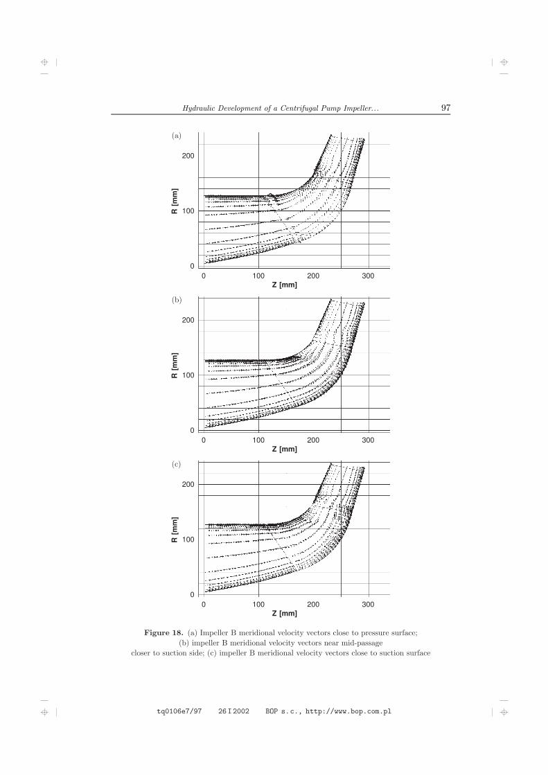
The results of these calculations for the final impeller B design are displayed inFigures 18–20. These figures are similar to Figures 13–15 for impeller A. Figures 18aand 18b show the meridional velocity vector distributions between the hub and shroudof impeller B at locations close to the blade pressure side and in the mid-passagelocation, respectively. Comparing these results with those for impeller A (Figures 13aand 13b), a more uniform distribution of meridional velocity can be observed in thecase of impeller B. The flow in the mid passage follows the impeller B channelin the streamwise direction. Flow patterns shown in Figure 18a and Figure 18c,close to the pressure and the suction sides of the blades, respectively, are typicalfor impellers with specific speeds similar to those for impeller A. The flow patternsare comparable to those presented by Goto [14], in which the flow in a mixed-flowimpeller was investigated using the same CFD solver, BTOB3D. It is apparent fromthe comparisons of Figures 14a and 14b (for impeller A) and Figures 19a and 19b (forimpeller B) that the meridional velocity is far more uniform for impeller B. Whilethe impeller B flow field is more uniform, impeller A has two levels of cross-passagevelocity, with high velocities close to the hub and low velocities and the beginning ofbackflow in the upper part of the passage and close to the shroud. The size of the



Figure 16. Meridional profile of impeller B with meshing for Q3D analysis

Figure 17. 3D digital impeller B model

local recirculation zone, which is created close to the impeller B shroud, is almostconstant in the pitchwise direction between the mid-pitch and the suction side of theblade (see Figures 21 and 22). The blade optimization, which consisted of systematicmodification and evaluation for several combinations of the shroud contour and theblade angle distribution along the shroud, resulted in the configuration in which theimpeller discharge recirculation zone was moved back from the trailing edge and islocated in the passage away from the impeller outlet plane. This relocation resultsin the decrease of the velocity gradient at the impeller B discharge plane and the



R[m

m]

200

100

00 100 200 300

Z [mm]

(a)

R[m

m]

200

100

00 100 200 300

Z [mm]

(b)

R[m

m]

200

100

00 100 200 300

Z [mm]

(c)

Figure 18. (a) Impeller B meridional velocity vectors close to pressure surface;(b) impeller B meridional velocity vectors near mid-passage

closer to suction side; (c) impeller B meridional velocity vectors close to suction surface



R[m

m]

200

100

00 100 200 300

Z [mm]

(a)R

[mm

]

200

100

00 100 200 300

Z [mm]

(b)

Figure 19. (a) Impeller B meridional velocity vectors at mid-passage;(b) impeller B meridional velocity distribution at mid-passage

S3 y

100

0

–100 0 100S3x

Figure 20. Impeller B meridional velocity distribution immediately after TE



Figure 21. Location of recirculation zone behind suction side of the blade close to TE and shroud

Figure 22. Location of the recirculation zone behind TE and suction side of impeller B

considerable reduction of the magnitude of the peak backflow velocity (by 66%) from−1.8m/s for impeller A to −0.67m/s for impeller B. Despite the existence of the localrecirculation zone, the flow pattern across impeller B remains more uniform both inthe streamwise and spanwise directions. The benefits of the performance enhancing



flow field features are confirmed by the increased efficiency, which is predicted to be0.902 for impeller B versus 0.869 for impeller A.

11. ConclusionsThe analysis of impeller A and the redesign effort for impeller B demonstrated

the potential for an improvement of the existing pump impeller using the integratedmodeling and flow simulation approach. The one-dimensional code was successfullyapplied to predict the design and off-design performance for the baseline pump withimpeller A. Detailed flow analysis and generation of the impeller with improvedefficiency required the combined use of the meanline code, design database for theimpeller sizing, plus Q3D and fully 3D viscous flow solvers to optimize the blading.The recirculation region exists in both impellers, but differs in the size and location,being closer to the shroud/suction side corner for impeller B with a less intense andreduced region of reverse flow near the exit. The main difference between the twoimpellers, however, is a much more uniform flow pattern in impeller B, both in thestreamwise and spanwise direction, and a considerable reduction of the cross flow inthe hub-to-tip direction. This reduction of the flow transport in the direction quasi-perpendicular to the mainstream direction results in the improvement in predictedefficiency for impeller B versus impeller A (from 0.869 to 0.902).

Further work in this project will include off-design performance analyses. Thedetailed study will include impeller-volute interaction and will require unsteady flowcomputations. This work is progressing and it will be reported separately.

References[1] Japikse D, Marscher W D and Furst R B 1997 Centrifugal Pump Design and Performance

Concepts ETI Inc.[2] Kaupert K 1997 Unsteady Flow Fields in a High Specific Speed Centrifugal Pump, PhD

Dissertation, ETH-Zurich[3] Japikse D 1987 ASME J. Turbomachinery 109 1[4] Japikse D 1991 Proc. Int. Symp. SYMKOM, Lodz, Poland, pp. 75–107[5] Howard J H G and Osborne C 1977 ASME J. Fluids Engineering 99 141[6] Howard J H G, Osborne C and Japikse D 1994 ASME Paper 94-GT-148[7] CCAD – User’s Guide, Concepts NREC[8] PUMPAL – User’s Guide, Concepts NREC[9] Denton J 1994 AGARD LS 195, Turbomachinery Design Using CFD

[10] Miner S M 1997 ASME Paper FEDSM97-3354[11] Dawes W 1987 IMechE Paper C267/87[12] Dawes W 1988 A Computer Program for the Analysis of Three-Dimensional Viscous Com-

pressible Flow in Turbomachinery Blade Row Whittle Laboratory, Cambridge University,UK

[13] Tsuei H H, Oliphant K and Japikse D 1999 Proc. IMechE Symp. CFD Technical Developmentsand Future Trends, London, UK

[14] Goto A 1990 ASME Paper 90-GT-36


HYDRAULIC DEVELOPMENT OF A CENTRIFUGAL PUMP … · A CENTRIFUGAL PUMP IMPELLER USING THE AGILE...

Documents

Transcript of HYDRAULIC DEVELOPMENT OF A CENTRIFUGAL PUMP … · A CENTRIFUGAL PUMP IMPELLER USING THE AGILE...