Hybrid Strategies for Adjoint

Methods in the Context of

Shape Optimization

Seminararbeit von

Fabian Key

(303550)

Juli 2014

Betreuer: Dipl.-Ing. M. Towara (STCE)

STCERWTH Aachen University

Germany

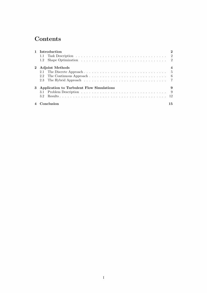
Contents

1 Introduction 2

1.1 Task Description . . . . . . . . . . . . . . . . . . . . . . . . . . . . . . . . . . 21.2 Shape Optimization . . . . . . . . . . . . . . . . . . . . . . . . . . . . . . . . 2

2 Adjoint Methods 4

2.1 The Discrete Approach . . . . . . . . . . . . . . . . . . . . . . . . . . . . . . . 52.2 The Continuous Approach . . . . . . . . . . . . . . . . . . . . . . . . . . . . . 62.3 The Hybrid Approach . . . . . . . . . . . . . . . . . . . . . . . . . . . . . . . 7

3 Application to Turbulent Flow Simulations 9

3.1 Problem Description . . . . . . . . . . . . . . . . . . . . . . . . . . . . . . . . 93.2 Results . . . . . . . . . . . . . . . . . . . . . . . . . . . . . . . . . . . . . . . . 12

4 Conclusion 15

I

List of Figures

1.1 Hicks-Henne bump functions h(x) =(

sin(πxlog 0.5

log a ))3

for a = 0.25, 0.5, 0.75 . 3

1.2 Optimization loop using an adjoint method . . . . . . . . . . . . . . . . . . . 3

2.1 Discretization and linearization compared for the discrete and continuousadjoint approach [6] . . . . . . . . . . . . . . . . . . . . . . . . . . . . . . . . 4

2.2 Simple comparison of the different approaches [6] . . . . . . . . . . . . . . . . 72.3 Schematic sketch of the hybrid adjoint approach [6] . . . . . . . . . . . . . . . 7

3.1 Computational mesh around the airfoil [6] . . . . . . . . . . . . . . . . . . . . 93.2 Surface sensitivity of drag coefficient [6] . . . . . . . . . . . . . . . . . . . . . 123.3 Shape sensitivity of drag coefficient [6] . . . . . . . . . . . . . . . . . . . . . . 133.4 Drag and lift coefficient during the shape optimization process [6] . . . . . . . 143.5 Comparison of original and optimized shapes after 10 design steps [6] . . . . . 14

II

List of Symbols

a Parameter of Hicks-Henne bump function.C Subscript for continuous approach.Cp Specific heat capacity for constant pressure.D Subscript for discrete approach.E Internal energy.F Flux term.f Function for eddy viscosity.F v1 First viscous flux term.F v2 Second viscous flux term.G Constraints.H Stagnation enthalpy.h(x) Hicks-Henne bump function.J Cost functional.L Lagrangian function.L Lagrangian function.M∞ Dimensionless freestream Mach number.n normal vector.p Static pressure.Pr Dimensionless Prandtl number.PrT Dimensionless turbulent Prandtl number.R Gas constant.N Continuous constraints or PDEs.R Discrete constraints or residuals.Re Dimensionless Reynolds number.T Static temperature.U State variables.u Velocity.V Lagrange multipliers or adjoint variables.α Design variables.α Angle of attack.β Switch for hybrid cost functional.Γ Boundary of domain.δij Kronecker delta function.δ() Continuous perturbation.∆() Discrete perturbation.δ,∆ () Hybrid perturbation.µ Laminar viscosity.µt Turbulent viscosity.µv1 First viscosity combination.µv2 Second viscosity combination.ρ Density.τ Stress tensor.φ Discrete adjoint variables.ϕ Hybrid adjoint variables.Ψ Discrete adjoint variables.Ω Computational domain.

1

1 Introduction

1.1 Task Description

This paper was produced during the summer term 2014 in the context of the CES Master

Seminar. The task was to deal with a topic of current research based on scientific papers.Emphasis should be put on a didactic and comprehensible description of the selected issue.

In this paper, the principles of adjoint based shape optimization are considered. Partic-ularly, the utilization of a hybrid adjoint approach is motivated and discussed. This workmainly presents the findings published by Taylor et al. [5],[6].

1.2 Shape Optimization

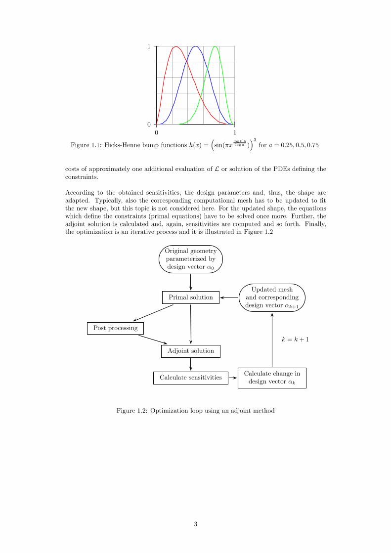
Shape optimization is the task to find a shape of a geometry that is optimal regardinga specific cost functional J . Typically, the shape has to satisfy a set of given constraintsG = 0 at the same time. Often, these constraints are defined by partial differential equations(PDEs) N = 0, which have to be fulfilled on the computational domain Ω. The optimizationproblem is discretized by introducing a parametrization of the shape which is defined by aset of design variables α. Depending on the choice of parametrization, the design variablescould be e.g. the parameters of Hicks-Henne sine bump functions [2] (see Figure 1.1) or thenormal displacement of surface mesh elements.The cost functional is typically defined over the domain Ω or the boundary Γ dependingboth on the state variables U and the design variables α:

J (U, α) on Ω or Γ (1.1)

The constraints can be combined as

G(U, α) = (N ) = 0 on Ω. (1.2)

The constrained problem

minα

J (U, α) subject to G(U, α) = 0 on Ω (1.3)

can be transformed into an unconstrained optimization problem by the so called method ofLagrange multipliers. The Lagrangian function is defined as

L = J + VTG, (1.4)

where V denotes the Lagrange multipliers which will be referred to as adjoint variables inthe following. For the solution of this problem, one can select an appropriate optimizationmethod. Here, we want to refer to gradient based optimization methods like the steepest de-scent method. For these methods, the gradient of the Lagrangian function L with respect todesign variables α is needed. It has as many entries as the number of design variables. Theindividual components are also called sensitivities, because they describe the change of thecost functional due to small changes in the corresponding design variable. One notes thatthe Lagrangian function consists of both the cost functional and the constraints defined byPDEs and, in general, depends on the design variables α as well as on the state variables U .

One way to calculate the sensitivities would be the finite differences approach. However, thecomputation of each component of the gradient would require the value of L and, thus, thesolution of a PDE system for a perturbation in one specific design variable. Therefore, theoverall effort for the gradient computation is proportional to the number of design variables.

Adjoint methods overcome this drawback and can provide sensitivity information at the

2

0

1

0 1

Figure 1.1: Hicks-Henne bump functions h(x) =(

sin(πxlog 0.5log a )

)3

for a = 0.25, 0.5, 0.75

costs of approximately one additional evaluation of L or solution of the PDEs defining theconstraints.

According to the obtained sensitivities, the design parameters and, thus, the shape areadapted. Typically, also the corresponding computational mesh has to be updated to fitthe new shape, but this topic is not considered here. For the updated shape, the equationswhich define the constraints (primal equations) have to be solved once more. Further, theadjoint solution is calculated and, again, sensitivities are computed and so forth. Finally,the optimization is an iterative process and it is illustrated in Figure 1.2

Original geometryparameterized bydesign vector α0

Primal solutionUpdated mesh

and correspondingdesign vector αk+1

Post processing

Adjoint solution

Calculate sensitivitiesCalculate change indesign vector αk

k = k + 1

Figure 1.2: Optimization loop using an adjoint method

3

2 Adjoint Methods

Adjoint methods can be used to obtain sensitivity information used in gradient based op-timization methods. One main advantage of these methods is that this information can beobtained at costs of one additional evaluation of L independent of the number of designvariables.

The underlying derivation is outlined in the following. The perturbation of the LagrangianδL arising from changes in the design α, which cause variations in the shape and, therefore,also in the state variables, is given as

δL = δJ + VT δG. (2.1)

We can expand the terms of equation (2.1) introducing the perturbations of the state vari-ables δU and those of the design variables δα. Factorizing yields:

δL =

(

∂J

∂α+ VT ∂G

∂α

)

δα+

(

∂J

∂U+ VT ∂G

∂U

)

δU (2.2)

Since we are still free in the choice of the adjoint variables V , we can make a demand on thesevariables such that the explicit dependence of δL on perturbations in the state variables δUvanishes. Otherwise, these dependencies would oblige us to recompute the solution for thestate variables for each perturbation in any design variable. These demands then result inthe adjoint equation

∂J

∂U+ VT ∂G

∂U= 0. (2.3)

If this equation and the constraints are fulfilled (G = 0 ⇒ L = J ), the sensitivities can becomputed according to

dJ

dα=∂J

∂α+ VT ∂G

∂α(2.4)

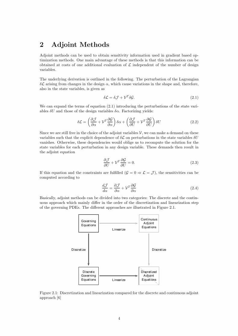
Basically, adjoint methods can be divided into two categories: The discrete and the contin-uous approach which mainly differ in the order of the discretization and linearization stepof the governing PDEs. The different approaches are illustrated in Figure 2.1.

Governing

Equat ions

Discrete

Governing

Equat ions

Cont inuous

Adjoint

Equat ions

Discret izedAdjoint

Equat ions

Discret ize

Linearize

Discret ize

Linearize

Figure 2.1: Discretization and linearization compared for the discrete and continuous adjointapproach [6]

4

2.1 The Discrete Approach

In the case of the discrete approach, the discrete adjoint system is derived based on thediscretized governing equations. Using the implementation of the solution scheme, Algo-rithmic Differentiation (AD) can be applied to get the required derivatives. Therefore, themathematical effort to obtain derivatives is relatively small and the results are exact up tomachine accuracy. Since the process can be automated, it can be easily applied to arbitrarycomplex cost functionals. On the other hand, high computational costs, especially memoryconsumption [7], may occur and one has only a slight flexibility regarding the solution ofthe arising systems which can become highly stiff or ill-conditioned [6].

The solution scheme for the discretized state equations should lead to vanishing residu-als everywhere in the computational domain. Since the boundary conditions already enterthe scheme, they are automatically contained. Therefore we have G = Rk = 0. TheLagrangian then reads

L = JD +N∑

k=1

ψTk Rk. (2.5)

One notes that we have L = JD, if the constraints are fulfilled, i.e. G = Rk = 0. For theperturbation one gets

∆L = ∆JD +

N∑

k=1

ψTk ∆Rk. (2.6)

The linearization of ∆JD and ∆Rk yields

∆JD =

N∑

l=1

DJD

DUl

∆Ul +DJD

Dα∆α (2.7)

∆Rk =

N∑

l=1

DRk

DUl

∆Ul +DRk

Dα∆α (2.8)

Plugging in this terms into equation (2.6) gives

∆L =

(

DJD

Dα+

N∑

k=1

ψTk

DRk

Dα

)

∆α +

N∑

k=1

(

DJD

DUk

+

N∑

l=1

ψTl

DRl

DUk

)

∆Uk (2.9)

As mentioned before, all terms which occur together with perturbations in the state variablesshould vanish. This leads to the adjoint equation

N∑

l=1

(

DRl

DUk

)T

ψl = −

(

DJD

DUk

)T

. (2.10)

If this equation is fulfilled, we can conclude for our cost functional

∆JD = ∆L =

(

DJD

Dα+

N∑

k=1

ψTk

DRk

Dα

)

∆α (2.11)

and further

dJD

dα=

DJD

Dα+

N∑

k=1

ψTk

DRk

Dα. (2.12)

The remaining terms are the explicit dependence of cost functional and state equationson the design variables. When the adjoint equation is solved, these dependences can becomputed relatively cheaply to obtain the sensitivity of the cost functional with respect tothe design variables.

5

2.2 The Continuous Approach

In case of the continuous approach, the analytical form of the state equations is used toderive the adjoint equations. The resulting system of equations is then discretized similarlyas it is done for the state equations. The derivation on an analytical level requires a lot ofmathematical effort and can become sophisticated for complex systems of state equations.However, one is free in the choice of a scheme for this system, since the obtained equationsdo not depend on the discretization of the state equations. On the other hand, the choiceof cost functionals is limited and the gradient can be inaccurate.

For the derivation of the continuous adjoint equations, we assume that the system of PDEsN is fulfilled, i. e. G = N = 0. Furthermore, the continuous objective function JC isdefined either over the whole computational domain Ω or over the boundary Γ. One canwrite

JC =

∫

Ω

jdΩ or JC =

∫

Γ

jdΓ. (2.13)

For the Lagrangian one gets

L = JC −

∫

Ω

φTNdΩ. (2.14)

A perturbation in the design α leads to perturbations in the state variables as well as in thecorresponding domain and boundary. For the perturbed Lagrangian it follows:

δJ = (J ′

c − Jc)−

(∫

Ω′

φTN ′dΩ−

∫

Ω

φTNdΩ

)

(2.15)

Again, the next step is to transform this equation such that terms including perturbationsin the state δU are isolated. Once this is done, one can set conditions such that these termsvanish. According to whether these conditions are defined over the domain or the bound-ary, they are referred to as adjoint equations or adjoint boundary conditions, respectively.Knowing or being able to easily calculate the remaining terms, one can now compute thesensitivity information of the objective function regarding changes in the design. Since thespecific state equations and boundary conditions directly enter equation (2.15), the deriva-tion of the adjoint equations cannot be generally done. One should note that each changein the state equations or boundary conditions requires a new derivation of adjoint equations.

To illustrate the proceeding, one part of the derivation for some flow equations is presentedin the following. For a stationary incompressible problem, the continuity equations for thestate variable U = u (velocity) is given as

N = −∂uj

∂xj= 0, (2.16)

where the Einstein notation was used. For the Lagrangian, it follows

L = JC +

∫

Ω

φTNdΩ. (2.17)

The derivative of L with respect to the i-th design variable αi is then given by

dL

dαi

=dJC

dαi

+d

dαi

(∫

Ω

φNdΩ

)

. (2.18)

With the Leibniz integral rule, it follows:

dL

dαi

=dJC

dαi

+

∫

Ω

φ∂N

∂αi

dΩ+

∫

Γ

φNnj

dxj

dαi

dΓ. (2.19)

The partial derivative of N with respect to the i-th design variable reads

∂N

∂αi

= −∂

∂αi

(

∂uj

∂xj

)

= −∂

∂xj

(

∂uj

∂αi

)

(2.20)

6

Thus, we have

∫

Ω

φ∂N

∂αi

dΩ = −

∫

Ω

φ∂

∂xj

(

∂uj

∂αi

)

dΩ, (2.21)

= −

∫

Γ

φ∂uj

∂αi

njdΓ +

∫

Ω

∂φ

∂xj

∂uj

∂αi

dΩ.

Now, we have isolated the terms corresponding to a perturbation in the state variables∂uj

∂αi

and we can set the multipliers to zero. For the field integral, we claim ∂φ∂xj

= 0. Together

with further conditions arising from the remaining state equations, the adjoint equations areobtained. Similarly, the terms of boundary integrals will lead to the boundary conditionsfor the adjoint variables.

2.3 The Hybrid Approach

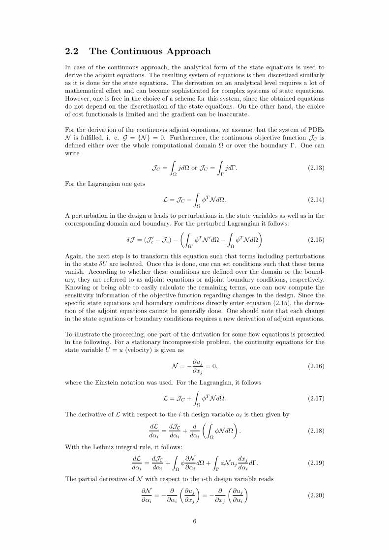
As mentioned before, the continuous and discrete adjoint approach often show opposingcharacteristics. The observed advantages and disadvantages of all approaches are listed inFigure 2.2. The hybrid approach mainly aims at combining these two approaches such that

Discrete Cont inuous Hybrid

Ease of development21, 22, 25–27 + ±

Compat ibility of numerical gradients:

- with the discret ized PDE9, 21, 26–28 +

- with the cont inuous PDE26, 29

Surface formulat ion for gradients28, 30

Ability to handle:

- arbit rary funct ionals22, 27

- non-di erent iability22, 26, 27, 31

Computat ional cost13, 21, 26, 27

Flexibility in solut ion21, 22, 26, 29, 32

Figure 2.2: Simple comparison of the different approaches [6]

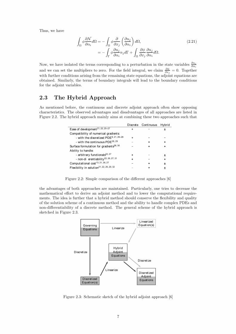
the advantages of both approaches are maintained. Particularly, one tries to decrease themathematical effort to derive an adjoint method and to lower the computational require-ments. The idea is further that a hybrid method should conserve the flexibility and qualityof the solution scheme of a continuous method and the ability to handle complex PDEs andnon-differentiability of a discrete method. The general scheme of the hybrid approach issketched in Figure 2.3.

Governing

Equat ions

Discret izedEquat ion(s)

LinearizedEquat ion(s)

Discret izedAdjoint

Equat ions

Hybrid

Adjoint

Equat ions

Discret ize

Linearize

Discret ize

Linearize

Figure 2.3: Schematic sketch of the hybrid adjoint approach [6]

7

For the hybrid approach the state equations are composed of one continuous and one discretepart, i.e.

G = NC , RkD = 0 (2.22)

The idea is then that equations which are not affected by small changes in the state equationsand which are easy to differentiate will enter the continuous part. The remaining equationswhich are not (easily) differentiable or are planed to be modified enter the discrete part. Ifone follows this approach and has once derived the continuous adjoint equations, variationsof the original problem will not require a huge development effort, but one will be allowedto reuse the majority of the already existing functionality. For the hybrid objective functiona combined version of continuous and discrete objective function is introduced:

JH = βJC + (1− β)JD (2.23)

This function is meant to be either fully continuous (β = 1) or fully discrete (β = 0). Thus,the variable β = 0, 1 serves as switch. The Lagrangian function containing both thecontinuous and discrete part of the state equations is given as:

L = βJC + (1− β)JD −

∫

Ω

ϕTCNCdΩ +

N∑

k=1

ϕTD,kRD,k (2.24)

The perturbation then yields

δ,∆L =β(J ′

C − JC) + (1 − β)∆JD (2.25)

−

(∫

Ω′

ϕTCN

′

CdΩ−

∫

Ω

ϕTCNCdΩ

)

+

N∑

k=1

ϕTD,k∆RD,k. (2.26)

The next step follows again the same idea as used before in the continuous and discrete ap-proach. Based on equation (2.26) one identifies terms containing perturbations in the statevariables δU and ∆U . Then, these terms have to vanish and thereby the adjoint equationand boundary conditions are obtained for the adjoint variables ϕC and ϕD.

Before one can start to derive a hybrid adjoint method for a specific problem, one hasmainly two degrees of freedom. The first one is the choice of the equations that enter eitherthe continuous or discrete part of the hybrid state equations. The second one is the decisionbetween a continuous or a discrete objective function.

8

3 Application to Turbulent Flow Simulations

3.1 Problem Description

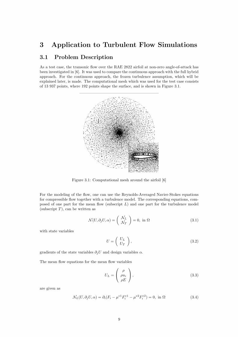
As a test case, the transonic flow over the RAE 2822 airfoil at non-zero angle-of-attack hasbeen investigated in [6]. It was used to compare the continuous approach with the full hybridapproach. For the continuous approach, the frozen turbulence assumption, which will beexplained later, is made. The computational mesh which was used for the test case consistsof 13 937 points, where 192 points shape the surface, and is shown in Figure 3.1.

Figure 3.1: Computational mesh around the airfoil [6]

For the modeling of the flow, one can use the Reynolds-Averaged Navier-Stokes equationsfor compressible flow together with a turbulence model. The corresponding equations, com-posed of one part for the mean flow (subscript L) and one part for the turbulence model(subscript T ), can be written as

N (U, ∂jU, α) =

(

NL

NT

)

= 0, in Ω (3.1)

with state variables

U =

(

UL

UT

)

, (3.2)

gradients of the state variables ∂jU and design variables α.

The mean flow equations for the mean flow variables

UL =

ρ

ρuiρE

, (3.3)

are given as

NL(U, ∂jU, α) = ∂i(Fi − µv1F v1i − µv2F v2

i ) = 0, in Ω (3.4)

9

with flux terms

Fi =

ρuiρuiuj + pδij

ρuiH

, F v1i =

0τijukτik

, F v2i =

00

Cp∂iT

. (3.5)

The stress tensor is defined by

τij = (∂jui + ∂iuj)−2

3δij∂kuk (3.6)

and the temperature for an ideal gas is given as

T =p

Rρ. (3.7)

For the viscosity terms we have

µv1 = µ+ µT , µv2 =

µ

Pr+

µT

PrT, (3.8)

with the laminar and turbulent Prandtl number Pr or PrT . The representation of the socalled eddy viscosity µT depends on the turbulence model. It is assumed that only µT cou-ples the mean flow equations and the turbulence model.

Next, a general representation for a turbulence model is given as

NT (U, ∂jU, α) = ∂iFTi− ST = 0, in Ω, (3.9)

with flux term FTiand source term ST . Depending on the specific model, this representation

contains one or multiple equations. The solution of these equations will then allow us tocompute the eddy viscosity µT and can in general depend on U, ∂jU and α.

The application of the continuous adjoint approach to a turbulence model is very challenging.A widely used assumption is that the variation of the eddy viscosity can be neglected and,thus, the influence on the sensitivities arising from the turbulence effects is dropped. Thisassumption is also known as the frozen turbulence assumption. However, for the Spalart-Allmaras model a continuous adjoint formulation was derived by Zymaris et al. [9].

One of the main achievements of the hybrid approach is now that one has the possibil-ity to treat the mean flow equations continuously and the equations of the turbulent modeldiscretely. This not only saves the effort for the analytical derivation of the continuous ad-joint equations but also lowers the costs for the adaption of the adjoint method in the case ofswitching the turbulence model. If one applies AD for the discrete part, the models can beseen more or less as black boxes. However, the mean flow equations still depend explicitlyon the eddy viscosity µT and, thus, also on the specific turbulence model. This remain-ing model dependence in the mean flow equations is removed by introducing an additionalequation for the eddy viscosity:

NµT (U, ∂jU, α) = µT − f = 0, in Ω (3.10)

with

f(U, ∂jU, α) = µT (3.11)

Thus, the explicit dependence on the form of µT is moved from the continuous to the discretepart.

Applying the steps described in the previous sections to this set of equations, one obtains acontinuous-like PDE with additional discrete and mixed source terms for the adjoint vari-ables corresponding to the mean flow. Additionally, one gets a set of hybrid boundaryconditions. These equations are solved like a traditional PDE. Furthermore, a discrete-likelinear system with mixed source terms can be derived for the turbulence related adjoint

10

variables and, again, this system is treated like a conventional linear system. It has to benoted that no model-dependent derivatives of the eddy viscosity appear in the continuouspart and, thus, these terms only enter the discrete part. Since AD can be used to computethe required derivatives, the mathematical form of the hybrid adjoint is not depending onthe specific turbulence model. Finally, the adjoint solution can be used to evaluate thesensitivity of the objective function with respect to changes in the surface shape of theairfoil.

11

3.2 Results

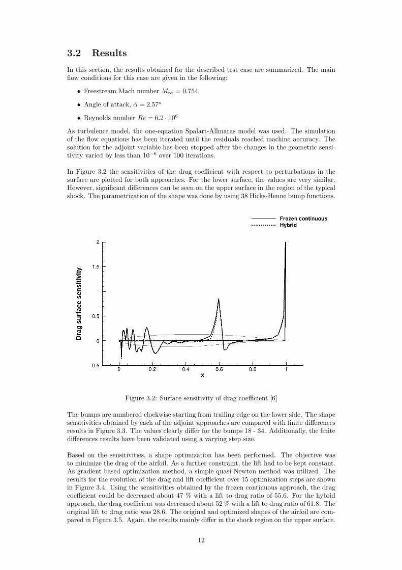
In this section, the results obtained for the described test case are summarized. The mainflow conditions for this case are given in the following:

• Freestream Mach number M∞ = 0.754

• Angle of attack, α = 2.57

• Reynolds number Re = 6.2 · 106

As turbulence model, the one-equation Spalart-Allmaras model was used. The simulationof the flow equations has been iterated until the residuals reached machine accuracy. Thesolution for the adjoint variable has been stopped after the changes in the geometric sensi-tivity varied by less than 10−6 over 100 iterations.

In Figure 3.2 the sensitivities of the drag coefficient with respect to perturbations in thesurface are plotted for both approaches. For the lower surface, the values are very similar.However, significant differences can be seen on the upper surface in the region of the typicalshock. The parametrization of the shape was done by using 38 Hicks-Henne bump functions.

Figure 3.2: Surface sensitivity of drag coefficient [6]

The bumps are numbered clockwise starting from trailing edge on the lower side. The shapesensitivities obtained by each of the adjoint approaches are compared with finite differencesresults in Figure 3.3. The values clearly differ for the bumps 18 - 34. Additionally, the finitedifferences results have been validated using a varying step size.

Based on the sensitivities, a shape optimization has been performed. The objective wasto minimize the drag of the airfoil. As a further constraint, the lift had to be kept constant.As gradient based optimization method, a simple quasi-Newton method was utilized. Theresults for the evolution of the drag and lift coefficient over 15 optimization steps are shownin Figure 3.4. Using the sensitivities obtained by the frozen continuous approach, the dragcoefficient could be decreased about 47 % with a lift to drag ratio of 55.6. For the hybridapproach, the drag coefficient was decreased about 52 % with a lift to drag ratio of 61.8. Theoriginal lift to drag ratio was 28.6. The original and optimized shapes of the airfoil are com-pared in Figure 3.5. Again, the results mainly differ in the shock region on the upper surface.

12

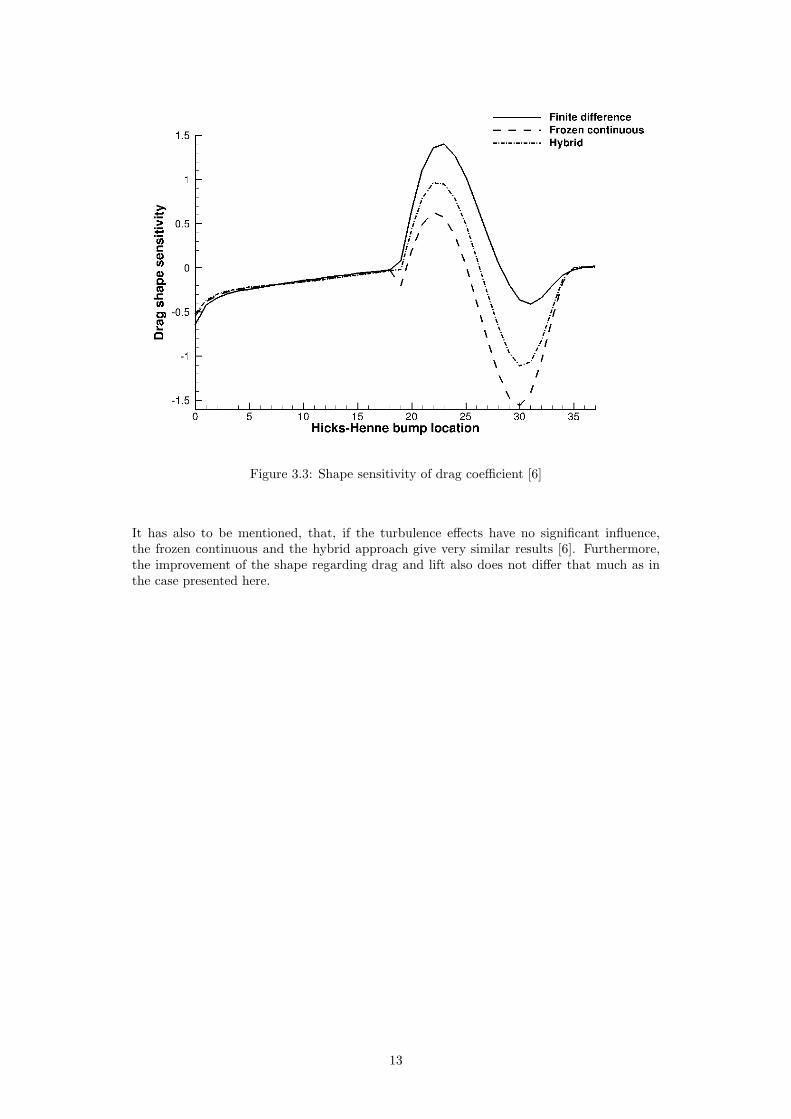
Figure 3.3: Shape sensitivity of drag coefficient [6]

It has also to be mentioned, that, if the turbulence effects have no significant influence,the frozen continuous and the hybrid approach give very similar results [6]. Furthermore,the improvement of the shape regarding drag and lift also does not differ that much as inthe case presented here.

13

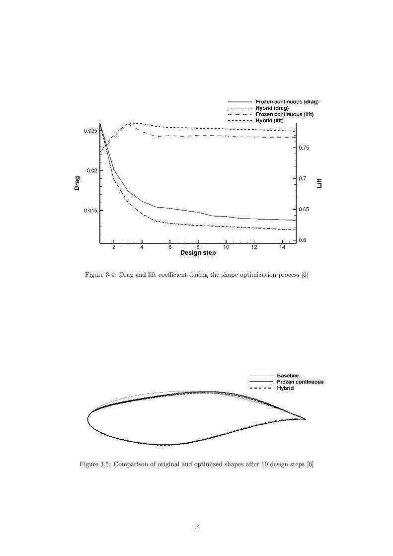
Figure 3.4: Drag and lift coefficient during the shape optimization process [6]

Figure 3.5: Comparison of original and optimized shapes after 10 design steps [6]

14

4 Conclusion

In this work, the basics of shape optimization have been described to motivate the use ofadjoint methods. A brief description of the discrete and continuous adjoint approach wasgiven. Based on the characteristics of both approaches, the idea and the motivation of ahybrid adjoint approach have been outlined. Finally, the application of this approach toa test case and the comparison of the obtained result with a classical adjoint approachhave been presented. One can conclude, that the main idea of a hybrid approach is tocombine the advantages of both the discrete and the continuous approach, e.g. loweringthe mathematical effort for its derivation and the computational requirements. This can beachieved by assigning equations that are not expected to change to the continuous part andtreating complex and varying parts of the problem discretely.

15

Bibliography

[1] R. E. Burkard and U. Zimmermann. Gradienten- und Newton-Verfahren. In Einfuhrung

in die Mathematische Optimierung, volume 5045 of Springer-Lehrbuch, pages 285–296.Springer Berlin Heidelberg, 2012.

[2] N. R. Gauger. Efficient Deterministic Approaches for Aerodynamic Shape Optimization.In D. Thevenin and G. Janiga, editors, Optimization and Computational Fluid Dynamics,pages 111–145. Springer Berlin Heidelberg, 2008.

[3] K. C. Giannakoglou and D. I. Papadimitriou. Adjoint Methods for Shape Optimization.In D. Thevenin and G. Janiga, editors, Optimization and Computational Fluid Dynamics,pages 79–108. Springer Berlin Heidelberg, 2008.

[4] C. Othmer. A continuous adjoint formulation for the computation of topological andsurface sensitivities of ducted flows. International Journal for Numerical Methods in

Fluids, 58(1770):861 – 877, 2008.

[5] T. W. Taylor, F. Palacios, K. Duraisamy, and J. J. Alonso. Towards a Hybrid AdjointApproach for Arbitrarily Complex Partial Differential Equations. In 42nd AIAA Fluid

Dynamics Conference and Exhibit, New Orleans, Louisiana, USA, 2012.

[6] T. W. Taylor, F. Palacios, K. Duraisamy, and J. J. Alonso. A hybrid adjoint approachapplied to turbulent flow simulations. In 21st AIAA Computational Fluid Dynamics

Conference, San Diego, CA, 2013.

[7] M. Towara and U. Naumann. A Discrete Adjoint Model for OpenFOAM. Procedia Com-

puter Science, 18(0):429 – 438, 2013. 2013 International Conference on ComputationalScience.

[8] M. Ulbrich and S. Ulbrich. Nichtlineare Optimierung. Mathematik Kompakt. SpringerBasel, 2012.

[9] A. Zymaris, D. Papadimitriou, K. Giannakoglou, and C. Othmer. Continuous adjointapproach to the spalartallmaras turbulence model for incompressible flows. Computers

& Fluids, 38(8):1528 – 1538, 2009.

16