Hybrid Solar-Fossil Fuel Power Generation

by

Elysia J. Sheu

Submitted to the Department of Mechanical Engineeringin partial fulfillment of the requirements for the degree of

Master of Science in Mechanical Engineering

at the

MASSACHUSETTS INSTITUTE OF TECHNOLOGY

T.ss~A TS INSTTUTE

OCT 2 2 2012

JBP A RESo__

September 2012

© Massachusetts Institute of Technology 2012. All rights reserved.

Author ... D............................ Ve pi f . .Departmeof

.X ... I..................

Mechanical EngineeringAugust 6, 2012

Certified by...............Alexander Mitsos

Rockwell International Assistant ProfessorThesis Supervisor

A ccepted by ........................... ..........David E. Hardt

Ralph E. and Eloise F. Cross Professor Of Mechanical EngineeringChairman, Department Committee on Graduate Theses

.. ................

2

Hybrid Solar-Fossil Fuel Power Generation

by

Elysia J. Sheu

Submitted to the Department of Mechanical Engineeringon August 6, 2012, in partial fulfillment of the

requirements for the degree ofMaster of Science in Mechanical Engineering

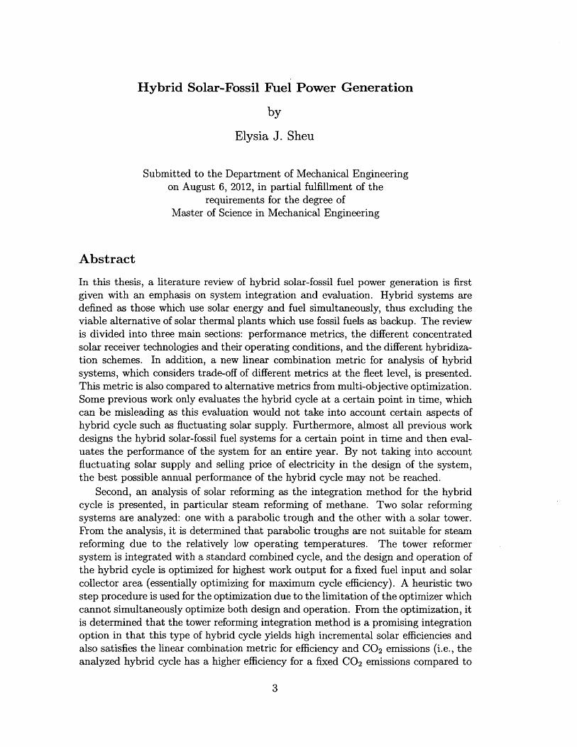
Abstract

In this thesis, a literature review of hybrid solar-fossil fuel power generation is firstgiven with an emphasis on system integration and evaluation. Hybrid systems aredefined as those which use solar energy and fuel simultaneously, thus excluding theviable alternative of solar thermal plants which use fossil fuels as backup. The reviewis divided into three main sections: performance metrics, the different concentratedsolar receiver technologies and their operating conditions, and the different hybridiza-tion schemes. In addition, a new linear combination metric for analysis of hybridsystems, which considers trade-off of different metrics at the fleet level, is presented.This metric is also compared to alternative metrics from multi-objective optimization.Some previous work only evaluates the hybrid cycle at a certain point in time, whichcan be misleading as this evaluation would not take into account certain aspects ofhybrid cycle such as fluctuating solar supply. Furthermore, almost all previous workdesigns the hybrid solar-fossil fuel systems for a certain point in time and then eval-uates the performance of the system for an entire year. By not taking into accountfluctuating solar supply and selling price of electricity in the design of the system,the best possible annual performance of the hybrid cycle may not be reached.

Second, an analysis of solar reforming as the integration method for the hybridcycle is presented, in particular steam reforming of methane. Two solar reformingsystems are analyzed: one with a parabolic trough and the other with a solar tower.From the analysis, it is determined that parabolic troughs are not suitable for steamreforming due to the relatively low operating temperatures. The tower reformersystem is integrated with a standard combined cycle, and the design and operation ofthe hybrid cycle is optimized for highest work output for a fixed fuel input and solarcollector area (essentially optimizing for maximum cycle efficiency). A heuristic twostep procedure is used for the optimization due to the limitation of the optimizer whichcannot simultaneously optimize both design and operation. From the optimization, itis determined that the tower reforming integration method is a promising integrationoption in that this type of hybrid cycle yields high incremental solar efficiencies andalso satisfies the linear combination metric for efficiency and CO2 emissions (i.e., theanalyzed hybrid cycle has a higher efficiency for a fixed CO 2 emissions compared to

3

a linear combination of solar only and fossil fuel only cycles).

Thesis Supervisor: Alexander MitsosTitle: Rockwell International Assistant Professor

4

Acknowledgments

The work presented here in this thesis would not have been possible without the

support of my family, friends, and colleagues. While it is impossible for me to thank

everyone, I would like to thank a few people in particular.

First and foremost, I would like to thank my advisor for all the time and effort he

has put into helping me with my work. Without his sacrifice, I would not have been

able to fully enjoy my research experience.

Secondly, I want to thank my parents for all the support and inspiration they have

given me and my brother for constantly being there whenever I need him. I want to

also thank my cousins for giving me their support.

Thirdly, I want to thank my coauthors and colleagues for their insightful discus-

sions which have benefited my work tremendously.

Finally, I would like to thank the King Fahd University of Petroleum and Minerals

in Dhahran, Saudi Arabia, for funding the research reported in this thesis through

the Center for Clean Water and Clean Energy at MIT and KFUPM under project

number R12-CE-10 and also Aspen Technology for generously providing the access

to AspenPlus®.

5

6

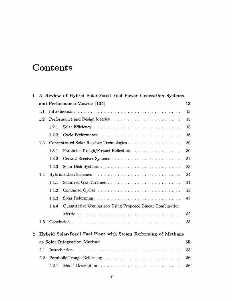
Contents

1 A Review of Hybrid Solar-Fossil Fuel Power Generation Systems

and Performance Metrics [105]

1.1 Introduction ....................

1.2 Performance and Design Metrics . . . . . .

1.2.1 Solar Efficiency . . . . . . . . . . .

1.2.2 Cycle Performance . . . . . . . . .

1.3 Concentrated Solar Receiver Technologies.

1.3.1 Parabolic Trough/Fresnel Reflectors

1.3.2 Central Receiver Systems . . . . .

1.3.3 Solar Dish Systems . . . . . . . . .

1.4 Hybridization Schemes . . . . . . . . . . .

1.4.1 Solarized Gas Turbines . . . . . . .

1.4.2 Combined Cycles . . . . . . . . . .

1.4.3 Solar Reforming . . . . . . . . . . .

13

. . . . . . . . . . . . 13

. . . . . . . . . . . . 15

. . . . . . . . . . . . 15

. . . . . . . . . . . . 16

. . . . . . . . . . . . 30

. . . . . . . . . . . . 30

. . . . . . . . . . . . 32

. . . . . . . . . . . . 33

. . . . . . . . . . . . 34

. . . . . . . . . . . . 34

. . . . . . . . . . . . 38

. . . . . . . . . . . . 47

1.4.4 Quantitative Comparison Using Proposed Linear Combination

M etric . . . . . . . . . . . . . . . . . . . . . . . . . . . . . . .

1.5 Conclusion . . . . . . . . . . . . . . . . . . . . . . . . . . . . . . . . .

52

53

2 Hybrid Solar-Fossil Fuel Plant with Steam Reforming of Methane

as Solar Integration Method 55

2.1 Introduction . . . . . . . . . . . . . . . . . . . . . . . . . . . . . . . . 55

2.2 Parabolic Trough Reforming . . . . . . . . . . . . . . . . . . . . . . . 56

2.2.1 Model Description . . . . . . . . . . . . . . . . . . . . . . . . 56

7

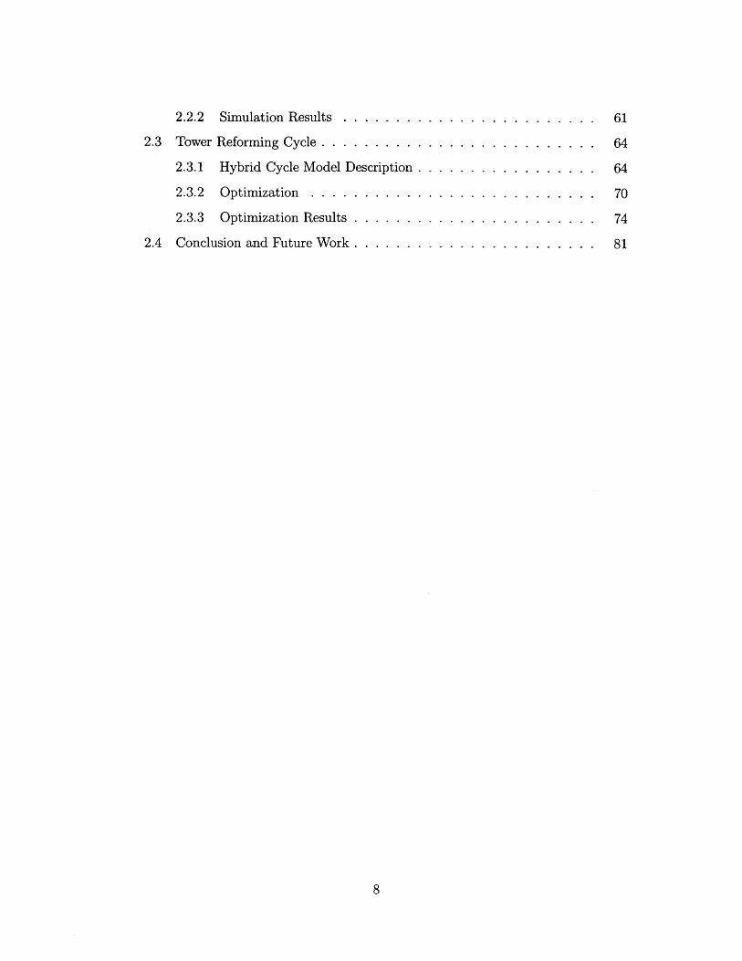
2.2.2 Simulation Results . . . . . . . . . . . . . . . . . . . . . . . . 61

2.3 Tower Reforming Cycle . . . . . . . . . . . . . . . . . . . . . . . . . . 64

2.3.1 Hybrid Cycle Model Description . . . . . . . . . . . . . . . . . 64

2.3.2 Optimization . . . . . . . . . . . . . . . . . . . . . . . . . . . 70

2.3.3 Optimization Results . . . . . . . . . . . . . . . . . . . . . . . 74

2.4 Conclusion and Future Work . . . . . . . . . . . . . . . . . . . . . . . 81

8

List of Figures

1-1 Fictitious example for linear combination metric: Assumed parameters

of solar only, fossil fuel only, and hybrid plants (Hybrid Cycle B is

competitive while Hybrid Cycle A is not) . . . . . . . . . . . . . . . . 29

1-2 Fictitious scenario for comparison of Pareto-optimal and linear combi-

nation metric (Pareto-optimal points are not necessarily optimal under

the metric proposed) . . . . . . . . . . . . . . . . . . . . . . . . . . . 30

1-3 Example of hybrid solar-fossil fuel gas turbine: Compressed air is

heated before entering the combustor and when solar energy is not

available, the air is directly sent to the combustor . . . . . . . . . . . 34

1-4 ORMAT hybrid solar-fossil fuel gas turbine schematic (adapted from

[36]) . . . . . . . . . . . . . . . . . . . . . . . . . . . . . . . . . . . . 36

1-5 Possible solar integration methods in a combined cycle: Solar heat

can be added to the top cycle, the bottoming cycle (preheating the

feedwater), or both (shown here) . . . . . . . . . . . . . . . . . . . . 39

1-6 Three different solar integration methods in the steam cycle (adapted

From [81]) . . . . . . . . . . . . . . . . . . . . . . . . . . . . . . . . . 47

1-7 General schematic of solar reforming . . . . . . . . . . . . . . . . . . 47

1-8 Schematic of solar syngas fired power plant (adapted From [119]) . . 50

1-9 Schematic of SOLRGT cycle (adapted from [131]) . . . . . . . . . . . 51

1-10 Trade off comparison between LEC and CO 2 emissions for various

power plants (Tunisia LEC includes subsidy for solar) . . . . . . . . 52

2-1 Cross-section of Parabolic Trough Receiver . . . . . . . . . . . . . . . 57

9

2-2 Trough Model Resistor Network . . . . . . . . . . . . . . . . . . . . . 58

2-3 Steam reforming model in Aspen Plus@ . . . . . . . . . . . . . . . . . 60

2-4 Trough outlet temperature vs. incidence angle . . . . . . . . . . . . . 62

2-5 Input water to fuel ratio for various reformer outlet temperatures . . 63

2-6 Power cycle flowsheet . . . . . . . . . . . . . . . . . . . . . . . . . . . 65

2-7 Reformer Temperature Variation (May 1) . . . . . . . . . . . . . . . . 67

2-8 Convection Heat Loss (Top in W) and Radiation Heat Loss (Bottom

in MW) Variation (May 1) . . . . . . . . . . . . . . . . . . . . . . . . 68

2-9 DNI trends throughout the day for various days in the year . . . . . . 69

2-10 Example of a "cloudy" day: DNI values much less than ideal . . . . . 70

2-11 Isentropic Efficiency Variation of Steam Turbines for May 1.. . . . . . 72

2-12 Solar Share Throughout Day (May 1) . . . . . . . . . . . . . . . . . . 75

2-13 Work Output Throughout Entire Year . . . . . . . . . . . . . . . . . 76

2-14 Comparison of Cycle and Incremental Solar Efficiency for May 1 . . . 76

2-15 Variation in Syngas (Reformate) Composition Throughout Day (Jan 1) 78

2-16 Comparison of Instantaneous Incremental Solar Efficiency: SR - Solar

Reforming and SCI - Steam Cycle Integration . . . . . . . . . . . . . 78

2-17 Comparison of Annual Incremental Solar Efficiency: SGT - Solarized

G as Turbine . . . . . . . . . . . . . . . . . . . . . . . . . . . . . . . . 79

2-18 Linear Combination Metric Comparison of Analyzed and Literature

Hybrid Systems with Solar Only Plant [33], State of the Art Natural

Gas CC [2], and Reference Plant . . . . . . . . . . . . . . . . . . . . . 80

10

List of Tables

1.1 Exergy values, LHVs, and fCO2 values of fuels most commonly used

in hybrid cycles (assumed composition of fuel in parentheses) [39, 68, 97] 20

1.2 Fictitious SLEC Example . . . . . . . . . . . . . . . . . . . . . . . . 24

1.3 Summary of performance metrics used in literature [16, 34, 100] . . . 26

1.4 Summary of design metrics used in literature [16, 34, 77, 100] . . . . 27

1.5 Summary of the different concentrated solar receiver technologies and

their operating conditions . . . . . . . . . . . . . . . . . . . . . . . . 31

1.6 Annual efficiency results for two solarized gas turbine cycles [100] . . 37

1.7 Economic analysis results for two solarized gas turbine cycles (total

cost including solar costs) [100] . . . . . . . . . . . . . . . . . . . . . 38

1.8 Efficiency comparison for three different hybrid combined cycles (shown

in Fig. 1-5) [80] . . . . . . . . . . . . . . . . . . . . . . . . . . . . . . 40

1.9 SMUD Kokhala thermal and economic analysis results for a solarized

gas turbine combined cycle [93] . . . . . . . . . . . . . . . . . . . . . 42

1.10 Layout of lowest LEC SCOT system for integration with a combined

cycle [62] . . . . . . . . . . . . . . . . . . . . . . . . . . . . . . . . . . 44

1.11 Performance of combined cycle in California for different operation

m odes [34] . . . . . . . . . . . . . . . . . . . . . . . . . . . . . . . . . 45

1.12 Currently existing hybrid solar-fossil fuel combined cycles [121] . . . . 48

2.1 Optical parameters for calculation of optical efficiency [37] . . . . . . 58

2.2 Nusselt number correlations for the convective resistances . . . . . . . 59

2.3 Parabolic trough parameters for simulation . . . . . . . . . . . . . . . 61

11

2.4 Energy breakdown for different processes in reformer . . . . . . . . . 64

2.5 Optimization Variables . . . . . . . . . . . . . . . . . . . . . . . . . . 73

2.6 Optimization Constraints . . . . . . . . . . . . . . . . . . . . . . . . . 73

2.7 Optimization Parameters . . . . . . . . . . . . . . . . . . . . . . . . . 74

2.8 Key Optimization Results . . . . . . . . . . . . . . . . . . . . . . . . 74

12

Chapter 1

A Review of Hybrid Solar-Fossil

Fuel Power Generation Systems

and Performance Metrics [105]

1.1 Introduction

As the world's population and economy continues to grow, electricity demand is

expected to continue to increase, leading to higher CO 2 emissions. In order to reduce

emissions, much research has been done investigating the use of renewable energy

sources, such as solar energy, for power production. Solar energy, at least in principle,

has the potential to provide all of the world's energy demands due to the large amount

of insolation available from the sun; however, at the present time, only a small amount

of the world's energy demand comes directly from solar energy. One reason for the

lack of solar energy utilization is that even at optimal locations, large collecting

areas are required which leads to higher costs as compared to other renewable/fossil

technologies [118]. Another reason is that the solar supply is variable through the

day which means that without some method of energy storage, power production

from solar is intermittent and not dispatchable. On the other hand, storage leads to

increased capital costs (even though the levelized cost can be lower with proper storage

13

[89, 12]). One potential solution to overcoming these intermittency and cost issues is

hybrid concentrated solar-fossil fuel power generation. Other hybrid concepts such as

solar with biomass fuel or solar with fossil fuel and wind are also promising, however,

this review will focus on hybrid solar-fossil fuel. Hybrid solar-fossil fuel generation

is defined here as a power cycle that whenever it utilizes solar energy, it also uses

fuel. This somewhat arbitrary definition excludes, for instance, a solar thermal plant

using fuel as backup when there is not enough solar insolation. Such concepts are

a promising option for solar utilization, but are excluded herein because these solar

thermal plants are already extensively reviewed in [13, 72, 120]. This review does

discuss some comparison between these hybrid and solar thermal plants (in particular

with the linear combination metric in Section 1.2), but a detailed comparison is

outside the scope of this review.

In addition to reduced fuel consumption and emissions as compared to fossil fuel

power generation [47, 116] and lower investment costs when compared to solar only

power plants, hybrid power generation has the following two main advantages: 1) It

is suitable for large-scale central electric power generation plants that can be inte-

grated into the power grid because it does not have the grid connectivity problems

(i.e., the need for synchronous reserve for frequency stabilization, fast power-ramping

rates, differences between times of peak supply and demand, etc.) that arise with

Concentrated Solar Power (CSP) or Photovoltaic (PV) plants without storage that

are subjected to interruptions and variable solar supply [123] and 2) the solar applica-

tion can be retrofitted to already-existing fossil fuel power plants (depending on site

resources and power cycle design). With regards to the first advantage, solar only

plants with proper storage or smart grid technology are also a promising option to

eliminate grid connectivity problems traditionally associated with solar [99].

Currently used or studied hybrid power generation processes can be grouped into

three main areas: solarized gas turbines, hybrid combined cycles, and solar reform-

ing. This article discusses these three main hybridization schemes with emphasis on

overall system design and integration, as opposed to, for example, solar reforming cat-

alysts. First, the different metrics typically used to characterize and evaluate hybrid

14

solar-fossil fuel system performance are discussed and a new metric for comparison

at the fleet level is proposed. Then, the different concentrated solar receiver tech-

nologies and their operating conditions are briefly discussed in order to illustrate how

different solar technologies should be primarily used for integration within a hybrid

cycle based on the temperatures required for the power generation. Finally, the three

main hybridization schemes are discussed.

1.2 Performance and Design Metrics

Within previous literature, many different metrics are used to characterize and eval-

uate hybrid cycles. However, there is not a single source where all these metrics are

presented and concisely explained and compared. In addition, some previous work

use these metrics to evaluate the performance of a hybrid cycle at a certain point

in time rather than over a time interval (which would take into account the fluc-

tuation of solar supply, the time value of electricity, and give more representative

results). Therefore, in addition to summarizing and explaining all previously used

metrics, time integral metrics are also given. Also, a new linear combination metrics

is proposed to allow for simultaneous evaluation of two metrics for a cycle.

The loss mechanisms associated with different solar technologies are first discussed

followed by a discussion of the thermodynamic and economic metrics, the time interval

metrics, and the new linear combination metric.

1.2.1 Solar Efficiency

Concentrated solar technologies are made up of two main components: the collectors

and the receivers. For example, in a parabolic trough, these are the parabolic solal

collectors and the receiver pipe. For each system there is an optical efficiency asso-

ciated with the collector and then there is a system efficiency which depends on the

optical efficiency as well as various loss mechanisms.

The main loss mechanisms for parabolic troughs and Fresnel reflectors (Section

1.3.1) include heat losses to the environment through convection and radiation. Also,

15

there are losses associated with the amount of radiation absorbed by the receiver

pipe, cosine losses, and the reflectivity of the mirrors. There is also the loss due to

the end effect, which is where, due to the tracking mode of the parabolic collector,

the solar irradiation ends up being focused a bit beyond the length of the receiver

tube. Spillage is a relative insignificant loss mechanism for parabolic troughs [57].

For the central receiver technologies (Section 1.3.2) loss mechanisms include heat

losses due to convection and radiation (like parabolic troughs), however, they are

significantly lower than the heat losses in a parabolic trough. There are also losses

due to radiation spillage, shadowing of the collectors by the receiver, atmospheric

attenuation, and blockage effects [46]. However, the main loss mechanism is due to

the cosine efficiencies of the heliostats.

Finally, for solar-dish (Section 1.3.3), loss mechanisms are similar to other CSP

technologies including heat losses and reflectivity losses [32].

All of these different loss mechanisms contribute to both the optical and system

efficiencies.

1.2.2 Cycle Performance

For hybrid concentrated solar-fossil fuel cycles a number of metrics are used to evalu-

ate cycle performance. These metrics can be grouped into first law efficiencies, second

law efficiencies, solar-related metrics, and economic metrics. Most metrics can be ei-

ther defined instantaneously or for a period of time (i.e., annualized). The metrics

definitions discussed herein will be for a single point in time and then a discussion

on how these metrics can be transformed into a metric for a period of time will be

presented. In addition, a new linear combination metric will be presented. A sum-

mary of the different metrics previously used in literature is shown in Tab. 1.3 and

Tab. 1.4.

Thermodynamic Metrics

First Law Efficiency

16

For a hybrid solar power cycle the first law system efficiency is defined as

91=*Qfuel+ Qsolar

where W is the net work output of the cycle, Ofuei is the "heating rate" input from

the fuel, and Qsolar is the energy rate input from the solar [16]. In the absence of

fossil fuel, this efficiency is the so called solar to electric efficiency.

The heating rate is defined as Qjuei = mfuel -LHV where LHV is the lower heating

value of the fuel (per unit mass) and fyhuei is the mass flow rate of the fuel used in the

cycle. Oolar is defined as Qsoar = 4 - Aa where 4 is the incident solar radiation and

Aa is the collector area. The reason to include the total area of collector in the solar

input calculation, e.g., as opposed to the solar heat reaching the cycle, is because

this represents the total heating rate to the system accounting for optical losses. In

addition, a substantial fraction of the capital cost is the collector area, which will only

be taken into account if the total collector area is used in the solar input calculation.

The first law system efficiency has also been defined without the solar input as

77I,no-solar -

Qfuel

However, this metric can be misleading since it is a monotonically increasing function

of solar share which will be defined later. It essentially considers the solar energy

to be "free" which is unrealistic. Moreover, this metric is very similar to the CO2

emissions metric (merely take the inverse of the fuel only efficiency and multiply by

the emissions of the fuel to get the CO 2 emissions), and therefore does not give any

new insight.

Second Law efficiency

The second law system efficiency for a hybrid solar power cycle is defined as

W711=II e koa

17

where Eyse, is the exergy rate of the fuel and Esoiar is the exergy rate of solar input

[16].

There are numerous ways of calculating solar exergy. One class of methods is to

consider a "thermodynamic system" where a certain volume is initially filled with

equilibrium blackbody radiation. The exergy of this system is then determined by

how much work can be extracted from this system as it reaches the "dead" state.

One common approach, within this first class, to calculating the exergy of the solar

input is as follows [55, 122]

Esolar = Neolar 1 -

where To is the ambient temperature and T is the temperature of the solar source

(temperature of sun surface ~ 5800K). Another similar method is suggested by Span-

ner as follows[109]

Esolar = Qsolar 4T

This method of calculation is similar to the first method discussed, however, 3/4

of the temperature of the sun surface is used (hence the factor of 4/3 in front of

the temperature ratio). A third method, within this first class of exergy calculation

methods, is suggested by Petela and is based on a quartic function for temperature

[86, 87]:1 (To 4TO

Esolar = Qsolar + ()43 T 3T

This quartic equation is based on the exergy of isotropic blackbody radiation for

a deformable reflecting enclosure and better represents the radiation that actually

reaches the earth's surface.

While these three methods of calculation may seem very different and contradict-

ing, Bejan argues that these three theories are in fact complementary. The differences

in each approach are due to the difference in understanding of how to describe the

"investment" made by thermal radiation in the production of work and how to ap-

propriately model the radiation system [19]. It is also important to note that for all

18

three estimations of the solar exergy, the exergy transfer rate is approximately equal

to the heat transfer rate (Eoiar ~ XQsoiar where x is between 93% and 95% ).

The second class of exergy calculation methods is to consider the emission of

solar radiation into the environment and determine how much mechanical power

can be produced with the portion of solar emission that can be intercepted by a

collector [19]. There are many models to approximate the collector which can be

found in [20]. One model is to assume that the collector is in thermal contact only

with the sun. In that case, for a given heat transfer rate Q the maximum power is

given by Q(1 - T) which can be used as the exergy. However, the maximum power

requires the collector temperature Tc to be equal to the sun temperature, implying

zero heat transfer per unit area. It is thus sensible to calculate the efficiency as

= ( - (T (1 - 1). For standard ambient conditions the maximum of

this expression is ~ 0.85 [20]. More complicated models account also for heat losses

to the ambient.

Recently Zamfirescu and Dincer [126] presented a method, wherein the solar ex-

ergy is also dependent on the solar constant, the solar insolation, and incidence angle.

This method gives lower values of exergy than most other methods discussed previ-

ously with exergy values being as low as 85% of the energy value for times near sunset

and sunrise. However, the lower fraction still does not give significantly different val-

ues for solar exergy and energy for the majority of the day.

The exergy of the fuel can be calculated based on the combustion reaction as

follows

( i= -AnG + To n ( x M (i~ t"'i ffuel

where (gel is the standard mass exergy of the fuel, ARGO' is the Gibbs Free Energy of

reaction at standard pressure and temperature, R is the universal gas constant, T, is

the ambient temperature, xi is the mass fraction of species i in the environment, MMeto

is the molar mass of all the species i combined, MMi is the molar mass of species i in

the environment, and vi is the stoichiometric coefficient of species i (species i refers to

all species in the combustion reaction except for the fuel) [21]. For this calculation,

19

water is considered to be in the vapor phase, which is consistent with the use of the

LHV.

The second law efficiency is in principle, a better measure of hybrid cycle efficiency

than the first law efficiency because it takes into account weighted contributions of

the two input sources. However, as seen in Tab. 1.1, for most fuels of interest, the

exergy of the fuel is approximately equal to the LHV. Therefore, since the solar exergy

is also approximately equal to the solar energy (as discussed before), the second law

efficiency is approximately equal to the first law efficiency for any hybrid system.

Table 1.1: Exergy values, LHVs, and fCO2 values of fuels most commonly used inhybrid cycles (assumed composition of fuel in parentheses) [39, 68, 97]

Fuel Exergy Value LHV (MJ/kg) fCO2 (kg C0 2 /MJ)(MJ/kg)

Natural Gas (CH 4) 52 50 0.055

Coal (C) 26 23 0.159

Oil (C8 Hi 8 ) 45.5 43 0.072

Solar-Related Metrics

For almost all solar-related metrics, a "reference" plant is used as part of the

metric. The "reference" plant is typically taken to be the highest efficiency plant

with the same flowsheet as the hybrid plant except there is no solar application. The

fuel type and fuel flow rate are the same for both, but the operating conditions are

not necessarily the same [100]. However, a better reference plant would be the highest

efficiency plant in general (i.e., for a hybrid combined cycle, the reference plant would

be a standard highest efficiency combined cycle rather than one that is exactly the

same as the hybrid plant) because this allows for comparison with traditional plants

in a more generalized sense rather than a specific case. In either case, the efficiency

of the reference plant is given by

ref

20

where Wref is the work output of the reference plant given the same input of fuel as

the hybrid plant.

A metric commonly used to characterize hybrid cycles is the solar share. The

solar share can be defined in two different ways: either based on the energy input or

the work output. The solar share based on the energy input is defined as [57]

X,, = . La

Qfuel + (sLar

For the work output basis, the solar share is defined as [100]

W - 77re! 5fuel LHVX ~= iV

7 W

where 7hfe, is the amount of fuel consumed by the hybrid cycle, llref is the efficiency

of the reference plant, and W refers to the work output of the hybrid cycle.

Solar share may have an upper limit significantly less than one due to the fact

that the power cycle will most likely run even when there is no solar. Also, note that

the output and input solar share are not the same unless the efficiencies of the hybrid

and reference plant are equal.

Another measure of performance of a hybrid cycle besides the cycle efficiency is

the net incremental solar efficiency which is defined as

W - 7refni7fuelLHV7 net-incr-solar

Qsolar

where m is the flow rate of the fuel, and qref is the overall net electric efficiency of

the "reference" plant [34].

This incremental solar efficiency can be negative for, e.g., insignificant output solar

shares, so therefore, this metric can be used to determine a bad integration method.

An example would be if the solar application was integrated in a gas turbine such that

the solar energy is used to heat the flue gases after combustion. In this case, since

the flue gases are already at high temperatures, which the solar application cannot

necessarily reach, the amount of heating supplied by the solar application would

21

be minimal, regardless of input solar share, unless the combustion temperature is

lowered. Therefore, with the lower combustion temperature, the overall efficiency of

the hybrid plant would decrease and no "extra" power would be produced leading to

a negative incremental solar efficiency. Therefore, the net incremental solar efficiency

would be negative since the work output from the hybrid plant would be less than

the reference plant.

Another design parameter traditionally used for solar applications is the solar

multiple. The solar multiple is defined as

SM = QsoarQpower-bock

where Qolar is the thermal power produced by the solar field at the design point and

Qpower-block is the thermal power (from solar) required by the power cycle at nominal

conditions [77]. The above definition is used for solar only plants, however, when

applied to a hybrid cycle, the solar multiple is not independent of the input solar

share, and therefore not a design metric likely to be used for hybrid cycles.

One other performance metric is the incremental CO 2 avoidance which is defined

as

AC0 2 ( -$e - fconlref

where fCO2 is the amount of CO 2 emissions per heating rate of fuel [100]. Values of

fCO2 for a few common fuels are given in Tab. 1.1. Similar to the incremental solar

efficiency, this metric can also be negative for poor designs.

In addition to these different solar-related metrics, the ecological footprint of the

solar application should also be taken into account. More specifically, the land area

needed for the solar field should be considered as this will not only affect the cost

of the solar application but also the use of this land for the solar field can compete

with other important land uses such as agriculture or wildlife. Concentrated solar,

like most renewable energy technologies, has low energy density and thus requires

large land areas, usually on the order of 15768 - 22776 m2 /MW [90]. However, one

22

advantage for solar in terms of land usage is that solar fields can be placed on hillsides

[42, 78, 107, 108] or in desserts, i.e., utilize land that is otherwise not very valuable.

Moreover, a recent proposal for a biomimetic heliostat layout greatly reduces land

area of central receiver solar plants while simultaneously increasing field efficiency for

power generation [79].

Economic Metrics

The most common evaluation parameter of economic performance is levelized elec-

tricity cost (LEC), which is expressed as

LEC _ 1y+ OMP + F"y

where Ip", is the annualized present value of total investment cost, OMpay" is the

annualized present value of the operating and maintenance cost, FP.y" is the present

value of the annual fixed cost, and Eg,n"' is the annual electricity output [34].

The solar LEC (SLEC) is the LEC of the electricity produced from the solar

application. The solar LEC can be calculated as

SLEC - LEC - [(1 - Xs,o) - LECrej]

This SLEC approximates the LEC of the electricity that is produced by only the solar

part of the hybrid plant. The second term of the numerator represents the LEC of the

electricity produced by the fuel in the hybrid plant, and the difference between the

total LEC and the LEC of the fuel portion is divided by the solar share to represent

the LEC of the portion of electricity produced by the hybrid plant from the solar part

[34, 54].

Herein, a different definition for SLEC is given as

S C (l' + OM"," + F" "),solarSLEG -. PV V an P

X,oEone""

This calculation of SLEC is different from the one presented in [34, 54] since the

23

output solar share does not necessarily represent the portion of total cost associated

with the solar. To illustrate that the two definitions are different, consider a fictitious

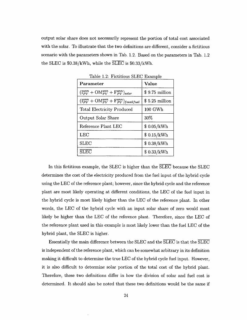
scenario with the parameters shown in Tab. 1.2. Based on the parameters in Tab. 1.2

the SLEC is $0.38/kWh, while the SLEC is $0.33/kWh.

Table 1.2: Fictitious SLEC Example

Parameter Value

(I "y"+ OMa"y"+ F)" )solar $ 9.75 million

(IP"y+ OMy+ F"y)fOssage $ 5.25 million

Total Electricity Produced 100 GWh

Output Solar Share 30%

Reference Plant LEC $ 0.05/kWh

LEC $ 0.15/kWh

SLEC $ 0.38/kWh

SLEC $ 0.33/kWh

In this fictitious example, the SLEC is higher than the SLEC because the SLEC

determines the cost of the electricity produced from the fuel input of the hybrid cycle

using the LEC of the reference plant; however, since the hybrid cycle and the reference

plant are most likely operating at different conditions, the LEC of the fuel input in

the hybrid cycle is most likely higher than the LEC of the reference plant. In other

words, the LEC of the hybrid cycle with an input solar share of zero would most

likely be higher than the LEC of the reference plant. Therefore, since the LEC of

the reference plant used in this example is most likely lower than the fuel LEC of the

hybrid plant, the SLEC is higher.

Essentially the main difference between the SLEC and the SLEC is that the SLEC

is independent of the reference plant, which can be somewhat arbitrary in its definition

making it difficult to determine the true LEC of the hybrid cycle fuel input. However,

it is also difficult to determine solar portion of the total cost of the hybrid plant.

Therefore, these two definitions differ in how the division of solar and fuel cost is

determined. It should also be noted that these two definitions would be the same if

24

the total cost of the reference plant is the same as the cost of the fossil fuel part of

the hybrid cycle. However, this would most likely not be the case as, for example,

if the solar is integrated into the steam cycle, the steam turbines would need to be

larger to accommodate the increase in steam flow rate, which would mean that the

cost of the fossil fuel portion of the hybrid cycle (the power cycle) would be higher

than the total cost of the reference plant (which would have smaller turbines).

Time Interval Metrics

Most metrics used in literature are for a certain point in time, however, a more

representative metric for evaluation would be one that is for a certain time interval

(in particular annual) because this would account for the fluctuation of solar. These

time interval metrics can be derived from the instantaneous definitions via an average

or weighted integral to take into account fluctuating solar supply, fuel price, and

electricity demand. The annual first law efficiency is shown below [100].

Wrq1 = Q5uei + Aa - fannDNI(t) dt

where W and Qfuei is the total work output and fuel input for the entire year, respec-

tively, and DNI is the direct normal irradiance as a function of time for the entire

year. Other annualized metrics are shown in Tab. 1.3 and Tab. 1.4.

The LEC is by definition annualized, but a better representation for cost may be a

LEC that takes into account time variations. In general, LEC is calculated by dividing

total cost of the plant by the amount of electrical energy produced by the plant.

However, the capital, operating, and maintenance costs are time-dependent (in that

present day value is used). Therefore, a time variable LEC would take into account

how valuable power is depending on demand, and therefore, this "worth" should be

factored into the calculation of the LEC through some weighted function for the power

produced that is dependent on time. There are also proposals for time dependent feed-

in tariff since these lead to more rational operation [41, 43]. Alternatively, the LEC

could also give some value to dispatchability (e.g., when energy is stored instead of

25

used immediately). Under rational energy policies, or in a free market with time-

variable electricity price, a plant with high LEC but dispatchable power can be more

profitable than plants with low LEC that cannot produce dispatchable power [94].

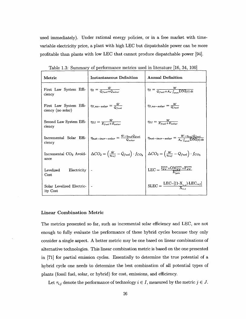
Table 1.3: Summary of performance metrics used in literature [16, 34, 100]

Metric Instantaneous Definition Annual Definition

First Law System Effi- rI - W = QfueL+Aa-f DNI(t) dtciency

First Law System Effi- 7 71,no-sol 7,no-solar = wciency (no solar)

Second Law System Effi- 11 = =Ef +eE +Esotrciency

Incremental Solar Effi- 7 net-incr-solar = "'reffuel 7 net incr-soar = Aa7f i(t) dt

ciency

Incremental CO2 Avoid- ACO2 = (7 - Ofue) - fco2 ACO2 = - fue) - fco2

ance

Levelized Electricity - LEC =- -1Cost """

Solar Levelized Electric- - SLEC = LEC "(X)LECr]

ity Cost X.'.

Linear Combination Metric

The metrics presented so far, such as incremental solar efficiency and LEC, are not

enough to fully evaluate the performance of these hybrid cycles because they only

consider a single aspect. A better metric may be one based on linear combinations of

alternative technologies. This linear combination metric is based on the one presented

in [71] for partial emission cycles. Essentially to determine the true potential of a

hybrid cycle one needs to determine the best combination of all potential types of

plants (fossil fuel, solar, or hybrid) for cost, emissions, and efficiency.

Let -rij denote the performance of technology i E I, measured by the metric j E J.

26

Table 1.4: Summary of design metrics used in literature [16, 34, 77, 100]

Metric Instantaneous Definition Annual Definition

Solar Share (input) XSi = o.. X,4 = Aa-fDNI(t) dt1.fuel+Qsolar Q uei+AaJanDN1(t) dt

Solar Share (output) X,,0 = Wre4f uel X = W-7ref Quel

Solar Multiple SM = Qsoar SM = AafnDNI(t) dtQpower-block Qpower-block

For simplicity, assume that the objective is to minimize all metrics (as opposed to

maximizing some). Typically, there are tradeoffs between different metrics, and not

all objectives can be simultaneously minimized. One way to deal with this tradeoff

is to assign weights to the different metrics and optimize for the weighted objective.

However, this is not desirable because it does not capture the tradeoffs, and the opti-

mal answer depends on the weights chosen. Instead, in multi-objective optimization

the notion of nondominated solutions or Pareto-optimal solutions is typically used,

e.g., [85]. If there are many competing technologies, a candidate technology n is

Pareto-optimal if and only if there exists no i E I such that

Vj E J : rij <; - ,j and 3j E J : ,j < Tnj.

In other words, to improve one of the metrics compared to technology n, another

metric will be deteriorated. There are techniques to calculate the set of Pareto optimal

solutions [66]. Pareto-optimization has been explored for power plants, e.g., in [67,

111, 38]. However, Pareto-optimality does not necessarily imply improvement over a

linear combination of alternative technologies. Herein, it is proposed to only choose

a technology if it improves one of the objectives compared to any possible linear

combination (more precisely convex combination), of alternative technologies, which

mathematically is expressed as: there exists no finite set i C I and A1 E [0, 1] with

27

E iAi= 1, s.t.:

Vj EJ:ZEAiTij : T 3, and 3j EJ:ZAi~i3 < Tn,j.

iEi iEi

The notion proposed is stronger than Pareto-optimal: a technology that satisfies the

above criterion automatically is also a Pareto optimal solution, but not vice-versa.

Another interpretation of the proposed metric is that it compares a given technology

with the convex hull of the Pareto front. As an example, consider that two objectives

are to be minimized, namely CO2 emissions per power produced, and LEC. A hybrid

plant must compete with fossil-fuel only plants and solar-only plants. Typically, fossil

fuel plants have significantly lower LEC and higher emissions than renewables, and

hybrid plants have intermediate values for both metrics

LECfossil < LEChybrid < LECsolar

CO2,solar < C0 2,hybrid < CO2,foss.

The hybrid cycle is a Pareto-optimal (nondominated) solution, since it can be seen

as an improvement over fossil fuel plant in terms of emissions, or as an improvement

over solar cycles in terms of LEC. However, the hybrid cycle needs to be compared

also to combinations of solar only and fossil only plants, and it is only viable if for

the same average LEC it has lower CO2 emissions

CO2,hybrid < CO2,fossil + LEChorid - LECfossi (CO2,solar - CO2,fossil)LECsolar -LECfosil

or equivalently, if for the same average CO 2 emissions it has lower LEC

LEChybrid < LECossal + CO2,hybrid - CO 2 ,fossal (LECsolar - LECfossL)CO2,solar - CO2,fossl

In other words, a hybrid cycle should improve on the two competing metrics at the

fleet level.

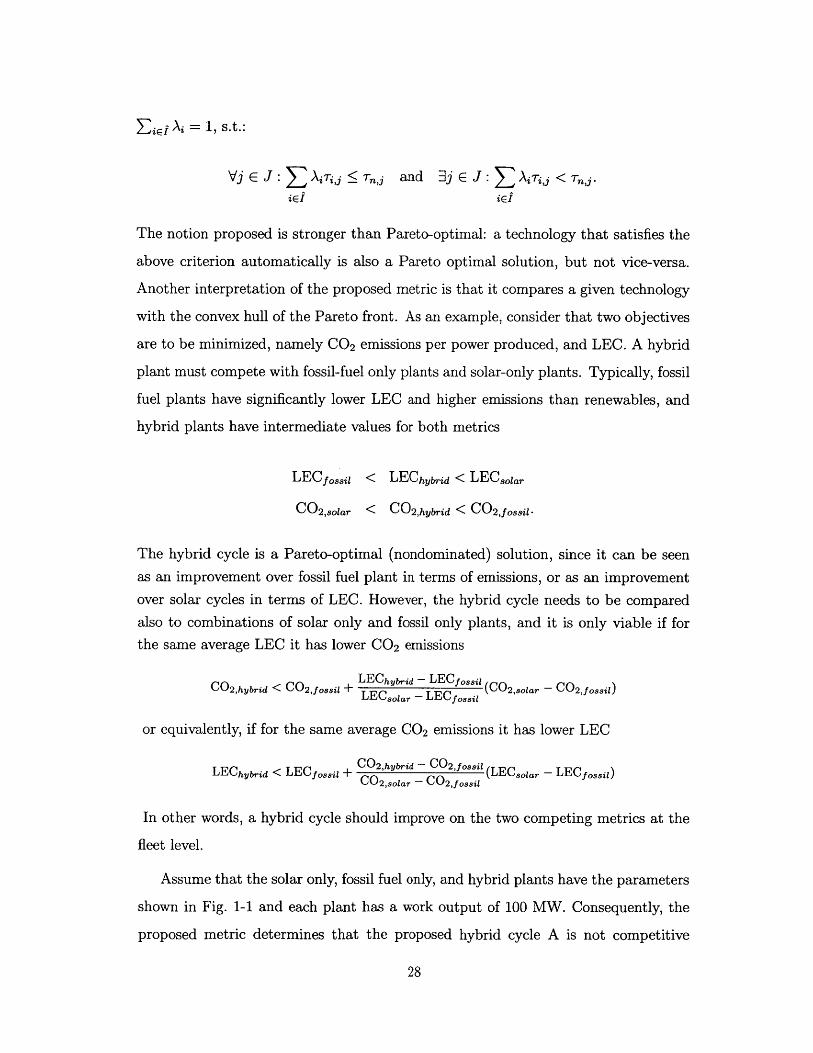
Assume that the solar only, fossil fuel only, and hybrid plants have the parameters

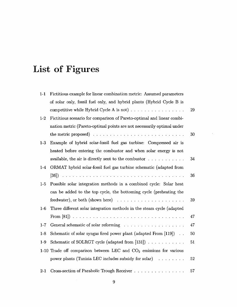
shown in Fig. 1-1 and each plant has a work output of 100 MW. Consequently, the

proposed metric determines that the proposed hybrid cycle A is not competitive

28

because if one has to provide 1 GW of power, instead of building ten hybrid solar-

fossil fuel A plants, one could build five solar only plants and five fossil fuel only

plants which would have the same amount of emissions with a lower average LEC

(0.13 $/kWh). Alternatively, one could build 6 solar only and 4 fossil fuel only plants,

and this combination would achieve approximately the same average LEC and less

overall emissions than 10 hybrid plants of technology A. In contrast, for hybrid cycle

B, the linear combination metric shows that this hybrid cycle is a viable one because

it gives a lower average LEC than a linear combination of the solar and fossil fuel only

plants with the same CO2 emissions or a lower CO 2 emissions for the same average

LEC. Note that similar to Pareto optimization, the proposed metric generates a set

of viable technologies, as opposed to a single optimal technology.

0.25

.2

02Solar Only

Hybrid Cycle A

U 0.1AFossil Fuel Only

0.05

00 0.1 0.2 0.3 0.4 0.5

CO2 Emissions (kg/kWh)

Figure 1-1: Fictitious example for linear combination metric: Assumed parametersof solar only, fossil fuel only, and hybrid plants (Hybrid Cycle B is competitive whileHybrid Cycle A is not)

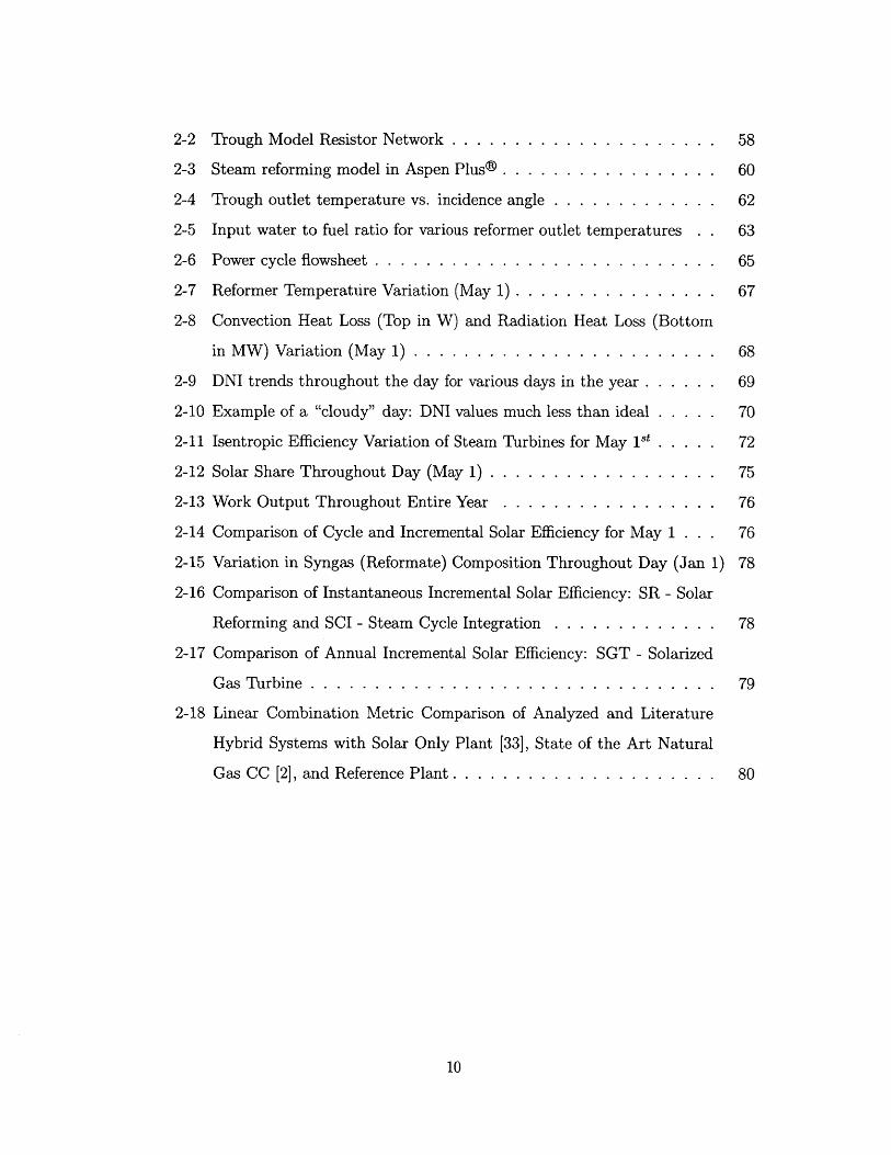
To demonstrate that the proposed metric is an extension of the notion of Pareto-

optimal solutions in multi-objective optimization, consider a fictitious scenario shown

in Fig. 1-2. Therein, Hybrid Plant C is on the Pareto-optimal front, however, Hybrid

Plant C should not be considered since a linear combination of solar only and fossil fuel

only plants will have the same emissions with a lower average LEC or the same average

LEC with lower emissions than Plant C. In other words, plant C is not dominated

29

by any single plant, but it is dominated by combinations and the proposed metric

compares the performance of a given plant at the fleet level. Rather than merely

optimizing a metric for a given plant, the most sensible use of resources is to consider

the cumulative effect of all plants in operation or planned.

0.25

0.2Solar Only

Hybrid Plant C

snPareto-optimal

Li& near CombinationU0.1LU

Fossil Fuel Only

0.05

00 0-1 0-2 0.3 0.4 03

CO2 Emissions (kg/kWh)

Figure 1-2: Fictitious scenario for comparison of Pareto-optimal and linear combi-nation metric (Pareto-optimal points are not necessarily optimal under the metricproposed)

1.3 Concentrated Solar Receiver Technologies

In this section, the concentrated solar receiver technologies and their operating condi-

tions will be discussed. A summary of the different technologies is shown in Tab. 1.5.

1.3.1 Parabolic Trough/Fresnel Reflectors

The parabolic trough technology is the most mature of the concentrated solar power

technologies. It uses a single-axis tracking curved mirror system to concentrate solar

radiation onto a receiver pipe which contains a heat transfer fluid. In most cases,

the heat transfer fluid used is either a mineral oil or a synthetic thermal oil. This

fluid is then most often used in a heat exchanger for steam generation [26]. Parabolic

troughs are also considered for direct steam generation where the fluid in the pipe is

30

Table 1.5: Summary of the different concentrated solar receiveroperating conditions

technologies and their

Technology Highest Re- Operating Most Stud-ported Solar Tempera- ied Inte-to Electricity tures grationEfficiency Method

for HybridCycles

Parabolic Trough 20% [33, 92] < 670 K [33, Supplemental92] Heat for

Steam Cy-cles [34, 28,75, 106, 35,125, 58]

Linear Fresnel Reflector 15% [65] < 520 K [65, Supplemental

73] Heat forSteam Cy-cles [74]

Central Receiver 23% [33] 850 K - 1070 PreheatingK [24, 25, 26, Compressed33, 54, 98] Air [25, 36,

93, 62]

Solar Dish 31.25% [9] 870K - 1020 Solar Re-K [33] forming

[70]

the working fluid (steam) of the power cycle [22, 73, 127]. Parabolic trough systems

can also be used with different types of thermal energy storage systems such as two

tank sensible heat systems, molten salt systems, phase-change systems [45, 49, 83],

solid media storage systems (like concrete) [63], and steam storage [76].

The operating temperatures of these parabolic trough systems can be as high as

approximately 670 K with a reported peak solar to electricity efficiency of about 20%

(see Section 1.2 for a formal definition) [33, 92]. Also, due to the relative maturity

and low price of this technology, a parabolic trough system is one of the more popular

options for use in a hybrid combined cycle. Parabolic troughs can be used to reheat

feedwater extracted from the Heat Recovery Steam Generator (HRSG), which in

turn increases the flow of steam into the steam turbine allowing for more power to

be produced with less fuel consumption [81]. However, due to the relatively low

operating temperatures, parabolic troughs may not be as suited for use in hybrid

31

Brayton cycles or in solar reforming [33].

Fresnel reflectors are similar to parabolic troughs in that solar radiation heats

a receiver pipe which contains the heat transfer fluid. In other words, both are

line-concentrating systems. However, instead of parabolic shaped mirrors, Fresnel

reflectors are long and narrow and have little to no curvature [74]. Fresnel reflectors

also differ from parabolic troughs in that the reflectors are composed of several long

row segments which then focus on elevated long receivers running parallel to the

rotational axis of the reflectors [73]. Fresnel reflectors also tend to be cheaper than

parabolic troughs (approximately 25% cheaper), however, they also tend to have lower

efficiencies as well (percent differences as high as 20%) [65].

It should also be noted that even though, as previously stated, both troughs and

Fresnel reflectors have relatively low operating temperatures and therefore may not be

as suited for use in hybrid Brayton cycles or in solar reforming, there is current work

being done with direct steam generation in troughs (described earlier) and Fresnel

reflectors that can allow these line-concentrating systems to operate at temperatures

as high as 773 K [22, 8]. These higher operating temperatures can potentially lead

to integration methods for troughs and Fresnel reflectors beyond just preheating or

reheating feedwater. However, increased costs, optical losses, and heat losses should

also be potentially considered.

1.3.2 Central Receiver Systems

Central receiver systems use a field of two-axes tracking heliostats to reflect solar

energy onto a single receiver or a small number of receivers. The most common

configuration are solar towers, where the receiver is mounted on the top of a tower

positioned at the center of or on one side of the field. A fluid is again used as the heat

transfer medium. Fluids used in solar tower systems include steam/water, molten

salts, liquid sodium, and air. A solar tower system also has the capability of energy

storage through the use of molten salts and two tank systems [26, 96].

These solar tower systems can traditionally reach operating temperatures of up

to 850 K with a reported peak solar to electricity efficiency of 23% (see Section 1.2

32

for a formal definition) [33]. However, research is being done on solar air-towers with

pressurized volumetric receivers combined with gas turbines that can reach operating

temperatures between 1020 K and 1200 K [24, 25, 26, 54, 98]. These volumetric

receivers operate by having a volume within the receiver made of various materials

such as ceramics, metal, and foam which absorbs the concentrated solar radiation

while the working fluid goes through the volume and is heated by forced convection

[15]. Recent research has also been done towards designing alternative volumetric

receivers that do not require a tower (i.e., all equipment including receivers are on

the ground) [42, 78, 107, 108]. With higher operating temperatures than the parabolic

troughs, solar towers are usually more suited for preheating the compressed air (either

directly or through a heat transfer fluid) in a hybrid Brayton or Combined cycle or,

depending on the reforming method, as the heat source for solar reforming.

1.3.3 Solar Dish Systems

One of the most common solar dish systems is the dish-engine. Dish-engine systems

are the most efficient of the receiver technologies in terms of the maximal achieved

conversion of solar energy into electricity (see Section 1.2 for formal definition). In

this system, the dish concentrator reflects solar rays onto a receiver located at the

focal point of the concentrator (usually parabolic). The receiver then uses the solar

energy to heat a gas (usually Helium or Hydrogen), which is then used as the working

fluid in an engine, e.g., Stirling engine, to produce power [26].

The highest reported solar to electricity efficiency (see Section 1.2 for formal def-

inition) for solar dish-engine systems is 31.25% [9]. Operating temperatures of this

system can reach as high as 1020 K [33]. The dish-engine system is also the least

mature of the receiver technologies and is modular in design with a single dish limited

to a capacity on the order of 10-50 kWe [33]. Therefore, at least in the near-term

future, solar dish-engine systems are more likely to be used in smaller, high-value

applications rather than large scale hybrid power generation plants.

However, solar dishes without the engines have been used as the heat source for

ammonia based thermochemical energy storage through the production of hydrogen

33

[70]. The solar dishes used for the thermochemical energy storage have reached op-

erating temperatures as high as 870 K [70]. Due to the relatively high temperatures,

solar dishes can be potentially be used in solar reforming systems.

1.4 Hybridization Schemes

In this section, the different hybridization schemes that have been previously proposed

will be discussed. As aforementioned, the three main schemes are: solarized gas

turbines, hybrid combined cycles, and solar reforming systems.

1.4.1 Solarized Gas Turbines

Modifications to Gas Turbine Systems for Hybrid Operation

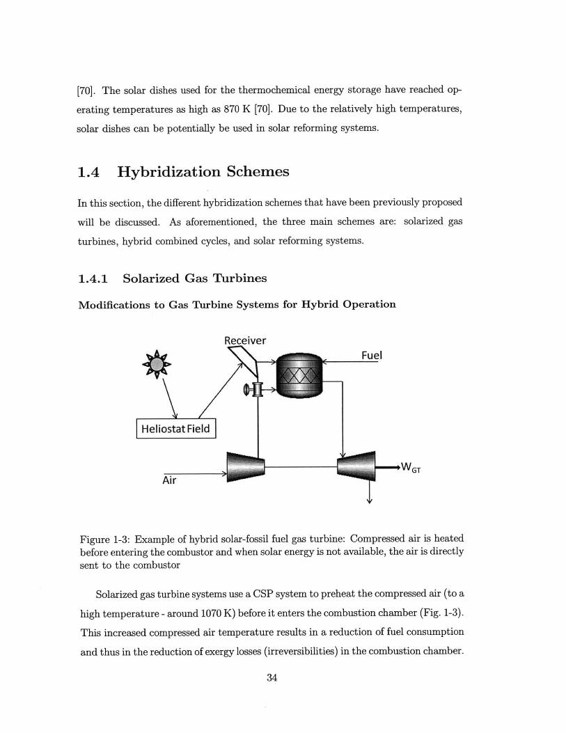
ReceiverFuel

Heliostat Field

-4WGT

Figure 1-3: Example of hybrid solar-fossil fuel gas turbine: Compressed air is heatedbefore entering the combustor and when solar energy is not available, the air is directlysent to the combustor

Solarized gas turbine systems use a CSP system to preheat the compressed air (to a

high temperature - around 1070 K) before it enters the combustion chamber (Fig. 1-3).

This increased compressed air temperature results in a reduction of fuel consumption

and thus in the reduction of exergy losses (irreversibilities) in the combustion chamber.

34

Consequently, this integration scheme can yield higher efficiencies (see Section 1.2 for

formal definition) - up to 30% when utilizing solarized gas turbines in a combined

cycle [36] - if the increased operating temperature does not yield significantly higher

solar to thermal losses. In particular, this arrangement can yield higher efficiencies

when compared to solar energy utilized in steam generation depending on the gas

turbine being used[80]. This higher solar to electric efficiency leads to a reduction

in the necessary heliostat field size which, in turn, leads to an overall reduction in

cost of the solar application. Also, with this integration method, the solar share

(formally defined in Section 1.2) is a function of the solar receiver outlet temperature

[25, 48]. This integration method also allows the power cycle to operate at full load

and efficiency even when there is no solar energy available [93].

Solarized gas turbines have been both modeled and built using solar towers with

different heat transfer fluids for the preheating process. Computer models of solar-

ized gas turbines have been created for a hybrid turbine with solar preheating from

a nitrate-salt solar tower [93] and turbines utilizing a solar tower with pressurized

volumetric receivers for preheating. These models will be discussed in more detail in

Sections 1.4.1 and 1.4.2. Maximum air preheating temperatures have reached a maxi-

mum of approximately 830 K for the nitrate-salt solar tower [93] while the preheating

temperatures for the tower with pressurized volumetric receivers have gone as high as

1070 K [24]. The higher temperatures associated with the volumetric receiver tower

makes it a more attractive option as the solar to electric efficiency would be higher;

however, turbine modifications are required for steady operation. An actual modified

gas turbine with the addition of the pressurized volumetric receivers was built and

tested, and the modification process and test results will now be discussed in detail

[36].

SOLGATE Project

The SOLGATE Project was started in 2002 by ORMAT industries to build a

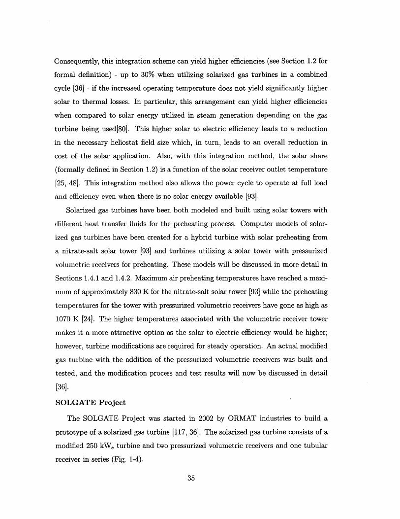
prototype of a solarized gas turbine [117, 36]. The solarized gas turbine consists of a

modified 250 kWe turbine and two pressurized volumetric receivers and one tubular

receiver in series (Fig. 1-4).

35

Fuel

Three Receivers In Series

Air WGT

Figure 1-4: ORMAT hybrid solar-fossil fuel gas turbine schematic (adapted from [36])

The volumetric receivers consist of a volumetric absorber and a domed quartz

window [24]. These receivers are tested in Spain at the Plataforma Solar de Almeria

(PSA) and the measured thermal efficiencies (defined as the amount of thermal energy

absorbed by the receiver minus the heat losses over the amount of incident solar

insolation available) of the receivers ranged from 63% to 75% with a pressure drop

across the receiver of 18 mbar [25].

The issues that arise with the incorporation of the volumetric receivers include a

higher combustor inlet temperature than traditional fossil-only plants and pressure

drops across the receiver [36]. To overcome these issues, the combustor is redesigned

with an in-line super alloy combustion chamber, a new air ducting system is added,

and a nitrogen purging system is added to prevent the injector from clogging [36].

The turbine was tested at PSA with 55 heliostats focused onto the receivers de-

livering approximately 1 MWth of solar power. The compressed air in the receiver

cluster is heated from 570 K to 1080 K and the hybrid gas turbine cycle has a first

law efficiency of approximately 20% (defined in Section 1.2) [36, 48].

The test shows that hybrid solar-fossil fuel gas turbine operation is conceptually

36

possible, however, this test was only done on a very small scale and further work

needs to be done in order to have this design realized on a larger scale.

Modeling of Solarized Gas Turbine Systems

In a study done by Schwarzb6zl et al. [1001, two industrial gas turbine systems were

chosen for technical and economic analysis as potential hybrid solar prototype plants:

1. Heron H1 - intercooled recuperated two-shaft engine with reheat and an ISO rating

of 1.4MW and 2. Solar Mercury 50 - recuperated single shaft gas turbine and an ISO

rating of 4.2MW.

The maximum receiver exit temperature is designed to be 1070 K and the systems

are analyzed for two different locations: Daggett, California and Seville, Spain. The

annual performance of the plant is calculated using the TRNSYS STEC software. A

typical meteorological year on an hourly basis is used for each location. The power

cycle efficiency results for 24 hour operation are shown in Tab. 1.6.

Table 1.6: Annual efficiency results for two solarized gas turbine cycles [100]Plant Power Cycle Efficiency (%)

Heron1 - Seville 40.4

Heron1 - Daggett 38.4

Mercury50 - Seville 35.9

Mercury50 - Daggett 35.9

The power cycle efficiencies (see Section 1.2 for formal definition) of the simulated

gas turbines are comparable to traditional fossil fuel Brayton cycles (both with re-

generation and without) [31, 30, 44, 124]. This comparison is made in relation to a

general high efficiency gas turbine cycle rather than to the exact same gas turbine

cycle without solar due to the fact that this comparison gives a better measure of the

potential of the hybrid system (see discussion of reference plant in Section 1.2). Pre-

sumably in [100] the efficiencies are calculated using the first law (see the discussion

on first vs. second law efficiencies in Section 1.2). Also, while this study does evaluate

annual performance, the design of the plant was still based on a certain point in time

rather than for an entire year.

37

For the economic analysis, an emerging market is assumed and the analysis covers

all expenses for engineering and development of the solarized gas turbine. It is also

assumed that the plant is fully operated by the staff on site. The solar field design is

cost optimized using HFLCAL code [18]. The levelized electricity costs are shown in

Tab. 1.7.

Table 1.7: Economic analysis results for two solarized gas turbine cycles (total costincluding solar costs) [100]

Plant LEC (o/KWh)

Heron1 - Seville 0.1913

Heron1 - Daggett 0.1993

Mercury50 - Seville 0.1004

Mercury50 - Daggett 0.0988

Solarized Steam Injection Gas Turbines

In addition to the solarized gas turbines discussed previously, there is also a solarized

steam injection gas turbine where the low temperature solar heat is used to create

steam which is then injected into the combustor in order to produce more power.

This solarized steam injection gas turbine has yielded first law efficiencies between 40

and 55%, incremental solar efficiencies between 22 and 37%, and input solar shares

of up to 50% [69]. The disadvantage of this type of gas turbine is that a low cost

condenser would be needed.

1.4.2 Combined Cycles

Many studies have been done regarding hybrid solar-fossil fuel combined cycles. The

main reason for this is that combined cycles have higher thermal efficiencies than

either Brayton or Rankine cycles. In particular, when integrating the solar application

with the gas turbine cycle, assuming a positive incremental solar efficiency (defined

in Section 1.2), these higher thermal efficiencies can lead to lower capital costs for

the integration of the solar application because less receiver/heliostat area would be

38

needed. Solar energy is typically incorporated into a combined cycle in two main

ways (usually one or the other but can be both): in the gas turbines as mentioned in

Section 1.4.1 or as supplemental solar heat to the bottoming Rankine cycle. There are

many different solar integration configurations for the bottoming cycle, and some of

the most studied methods for this type of integration in literature include preheating

the steam, extracting steam from the HRSG for reheating, and increasing the flow

rate of hot gas into the HRSG by supplementing the flue gas from the gas turbine

with air heated by the solar application. A few hybrid solar-fossil fuel combined cycles

are also currently being built in Egypt, Algeria, and Morocco [121].

Various studies have also been conducted concerning solar hybrid combined cycles

with some form of CO2 capture [53, 61, 84]. However, the focus here will be on the

integration of the solar application into the combined cycle.

Comparison of Different Integration Methods

R iver

Heliostat Field WST

Air HRSG Exhaust

Fedater

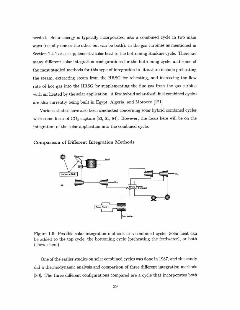
Figure 1-5: Possible solar integration methods in a combined cycle: Solar heat canbe added to the top cycle, the bottoming cycle (preheating the feedwater), or both(shown here)

One of the earlier studies on solar combined cycles was done in 1987, and this study

did a thermodynamic analysis and comparison of three different integration methods

[80]. The three different configurations compared are a cycle that incorporates both

39

the preheating of compressed air and supplemental heat to the Rankine cycle called

Plant A (Fig. 1-5), a cycle with just the supplemental heat called Plant B (Fig. 1-5

without the solar preheating of air), and a cycle with just the preheating of air called

Plant C (Fig. 1-5 without the solar in the bottoming cycle) - the configuration of

which was first suggested in 1979 [64]. In [80], both an energy and exergy analysis

was performed. The definitions for energy and exergy efficiency are discussed in

Section 1.2. The overall efficiencies of all three plants, taking into account combustion,

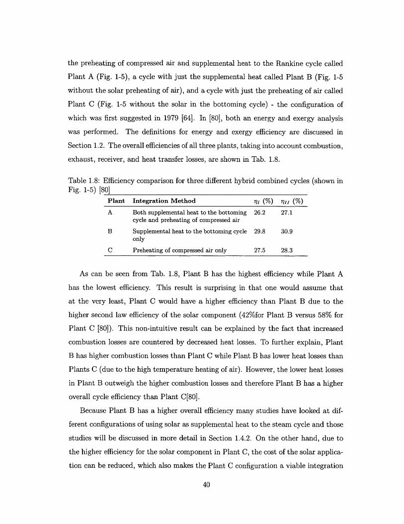
exhaust, receiver, and heat transfer losses, are shown in Tab. 1.8.

Table 1.8: Efficiency comparison for three different hybrid combined cycles (shown inFig. 1-5) [80]

Plant Integration Method r7 (%) 771 (%)

A Both supplemental heat to the bottoming 26.2 27.1cycle and preheating of compressed air

B Supplemental heat to the bottoming cycle 29.8 30.9only

C Preheating of compressed air only 27.5 28.3

As can be seen from Tab. 1.8, Plant B has the highest efficiency while Plant A

has the lowest efficiency. This result is surprising in that one would assume that

at the very least, Plant C would have a higher efficiency than Plant B due to the

higher second law efficiency of the solar component (42%for Plant B versus 58% for

Plant C [80]). This non-intuitive result can be explained by the fact that increased

combustion losses are countered by decreased heat losses. To further explain, Plant

B has higher combustion losses than Plant C while Plant B has lower heat losses than

Plants C (due to the high temperature heating of air). However, the lower heat losses

in Plant B outweigh the higher combustion losses and therefore Plant B has a higher

overall cycle efficiency than Plant C[80].

Because Plant B has a higher overall efficiency many studies have looked at dif-

ferent configurations of using solar as supplemental heat to the steam cycle and those

studies will be discussed in more detail in Section 1.4.2. On the other hand, due to

the higher efficiency for the solar component in Plant C, the cost of the solar applica-

tion can be reduced, which also makes the Plant C configuration a viable integration

40

method. Therefore, in order to truly determine which configuration is more suitable,

[80] suggested an economic analysis should be done in addition to a thermodynamic

one.

Since the publication of [80], many improvements have been made in terms of

turbomachinery (higher allowed inlet temperatures and better isentropic efficiencies)

and combined cycle configuration (use of reheat) [29]. All of these improvements lead

to higher efficiencies which means that calculated efficiencies of current cycles will

be higher than the ones calculated in [80]. However, the efficiency comparison would

most likely be the same because both gas turbine and steam turbine technologies have

improved since [80] was published.

Combined Cycle with Solar Integration in Gas Turbine

SMUD Kokhala Study [93]

In 1996, NREL and the Sacramento Municipal Utility District (SMUD) conducted

a conceptual evaluation of a 30.5 MWe combined cycle plant that uses a nitrate-salt

solar tower with a salt/air heat exchanger to heat the compressed air at the gas

turbine combustor inlet during peak solar insolation conditions.

The combined cycle uses a Westinghouse WR 21 gas turbine and due to the lack

of design data, the cycle design configuration is developed by the GateCycle program.

The cycle has a design point solar contribution of 18MWt or approximately 27% of

the total thermal input to the gas turbine.

Eight different solar plants ranging from 10 to 70MWt were designed for the

integration with the combined cycle. All the solar plants use a Solar-Two type nitrate-

salt external receiver with a solar field of 50m 2 heliostats. The DELSOL3 computer

code [59] is used to design the receiver diameter and height, tower height, and number

of heliostats for lowest energy costs. The location for the design is Daggett, California,

and the design uses a constant direct normal insolation of 950W/m 2 .

The annual thermal performance of the solar plants were modeled using SOL-

ERGY [1151. Although SOLERGY is most often used to calculate electricity output,

in [93], it was used to determine the thermal delivery of the solar plant to the com-

41

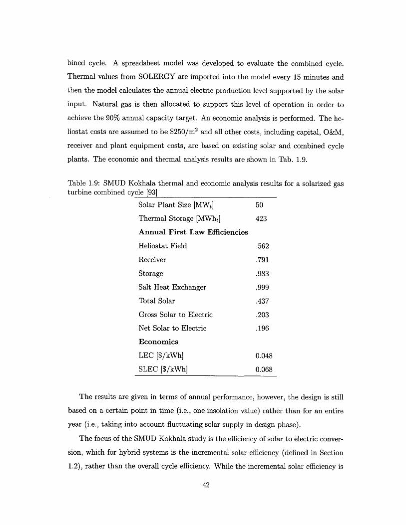
bined cycle. A spreadsheet model was developed to evaluate the combined cycle.

Thermal values from SOLERGY are imported into the model every 15 minutes and

then the model calculates the annual electric production level supported by the solar

input. Natural gas is then allocated to support this level of operation in order to

achieve the 90% annual capacity target. An economic analysis is performed. The he-

liostat costs are assumed to be $250/m 2 and all other costs, including capital, O&M,

receiver and plant equipment costs, are based on existing solar and combined cycle

plants. The economic and thermal analysis results are shown in Tab. 1.9.

Table 1.9: SMUD Kokhala thermal and economic analysis results for a solarized gasturbine combined cycle [93]

Solar Plant Size [MWt] 50

Thermal Storage [MWhtI 423

Annual First Law Efficiencies

Heliostat Field .562

Receiver .791

Storage .983

Salt Heat Exchanger .999

Total Solar .437

Gross Solar to Electric .203

Net Solar to Electric .196

Economics

LEC [$/kWh] 0.048

SLEC [$/kWh] 0.068

The results are given in terms of annual performance, however, the design is still

based on a certain point in time (i.e., one insolation value) rather than for an entire

year (i.e., taking into account fluctuating solar supply in design phase).

The focus of the SMUD Kokhala study is the efficiency of solar to electric conver-

sion, which for hybrid systems is the incremental solar efficiency (defined in Section

1.2), rather than the overall cycle efficiency. While the incremental solar efficiency is

42

important when evaluating a configuration, it should be evaluated in conjunction with

the cycle efficiency in order to take into account the usage of fuel and to determine

the true performance of the plant.

Kribus et al. Study [62]

Kribus et al. [62] also analyzed a combined cycle with solar heating of the com-

pressed air in the Brayton Cycle. The difference compared to [93] is that instead

of using a nitrate-salt solar tower with a heat exchanger, a Solar Concentration Off-

Tower (SCOT) and high temperatures receivers is used. The SCOT is different from

a traditional solar tower in that there is a reflector atop the tower which redirects the

solar radiation towards a focal region near ground level.

The hybrid solar combined cycle is designed using a modified DELSOL3 program

called WELSOL. WELSOL adds a SCOT optic model and additional options for

receivers, hybrid operation, and power generation to the DELSOL3 code. In addi-

tion, the WELSOL code includes calculation of losses due to the additional optical

elements, models of the performance of the high temperature receivers, gas turbine

and combined cycle performance models, and cost models for new components (i.e.,

additional reflectors, receivers, etc.).

Using WELSOL, the system is designed for the lowest LEC; however, in order to

improve computation speed, the physical models used in the WELSOL code are sim-

plified. To more accurately simulate the performance of the systems, two other codes

are used to simulate the system and these results from the more-detailed simulation

are used to validate the performance predictions of the optimized systems generated

from WELSOL. For the more-detailed simulation, the optics are simulated using a

statistical ray-tracing code called WISDOM [101] and then the output of the optics

simulation are used as input in the thermal analysis code ANN, which simulates the

performance of receivers, power conversion systems, and annual integration.

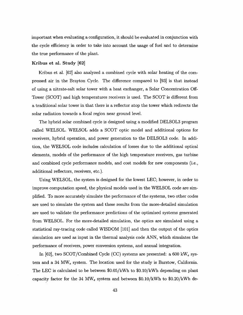
In [62], two SCOT/Combined Cycle (CC) systems are presented: a 600 kWe sys-

tem and a 34 MWe system. The location used for the study is Barstow, California.

The LEC is calculated to be between $0.05/kWh to $0.10/kWh depending on plant

capacity factor for the 34 MWe system and between $0.10/kWh to $0.20/kWh de-

43

pending on plant capacity factor for the 600 kW, system. Other results from the

optimization of the SCOT/CC system are shown in Tab. 1.10.

Table 1.10: Layout of lowest LEC SCOT system for integration with a combinedcycle [62]

Plant Rating 0.6 MWe 34 MWe

Number of Heliostats 48 1323

Tower Height [m] 49 163

Tower Reflector Area [m2 ] 190 3270

Turbine Inlet Temperature [K] 1273 1473

Gross Power Conversion Efficiency .356 .470

Annual Solar to Electric Efficiency .161 .213

Solar Capacity Factor .220 .242

Specific Cost [$/kW] 3943 2588

The performance calculations are based on an energy analysis as opposed to an

exergy analysis (see discussion in Section 1.2). [62] also suggests a size optimization

study should be performed in order to determine the optimal size of a SCOT plant

that can be implemented with a combined cycle.

Other Studies

Another study done by Segal and Epstein optimizes a combined cycle with a

solarized gas turbine for maximum efficiency [103] with a focus on determining the

best solar receiver temperature for efficiency. The efficiencies for a hybrid solar-fossil

fuel combined cycle range from 35% to 55% for solar receiver temperatures between

1000 K and 2000 K [103]. However, receiver temperatures of 2000 K are most likely

unrealistic as the highest reported receiver temperature is approximately 1300 K with

realistic operating temperatures around 1100 K [24].

Kakaras et al. [56] considered a combined cycle with wet gas turbine technologies

which uses the solar heat to evaporate water injected into the compressed air before

it enters the combustion chamber [56]. Although this cycle shows improvements for

both efficiency and cost on a small scale, [56] concludes that it is not likely to be

44

applied on a large scale due to the increased cost.

Combined Cycle with Solar Integration in Steam Cycle

Many different studies have looked at the integration of solar into the steam cycle

of the combined cycle in a variety of ways. An economic analysis for Egypt was

performed on two different hybrid combined cycles. The first cycle analyzed uses a

parabolic trough system to preheat a fraction of the feed water in a solar boiler, and

the second cycle uses a solar-air tower to heat air to temperatures higher than those

of the exhaust gas from the gas turbine and then the heated air is mixed with the

exhaust gases before entering the HRSG. While the economic analysis found a LEC

comparable to the LEC of a traditional fossil fuel plant, the solar share that produces

this LEC is not given, so it is unclear if this low LEC includes a significant solar

share.

The integration method of mixing solar-heated air with the exhaust gas of the

turbine before it enters the HRSG has also been considered for cogeneration power

plants [14].

Another study done in California also analyzed a CC with a parabolic trough

system that preheats some of the feedwater [34]. A duct burner is used as backup

when solar energy is not available. The efficiencies for the plant and solar shares

(defined in Section 1.2) for various situations are shown in Tab. 1.11. This study

is one of the few where both design and performance evaluation takes into account

fluctuating solar supply.

Table 1.11: Performance of combined cycle in California for different operation modes[34]

Solar/Duct Capacity [%] 100/0 50/0 50/50 0/100

Steam Cycle Efficiency [%] 37.5 36.72 36.98 37.61

Solar Share [%] 17.57 9.32 4.08 0

Fuel Based Net Electric Efficiency [%] 66.42 62.21 58.80 52.23

An exergy and energy analysis was also performed on a hybrid solar combined cycle

in Yzad, Iran [16]. In this case, the solar energy is used to reheat extracted feedwater

45

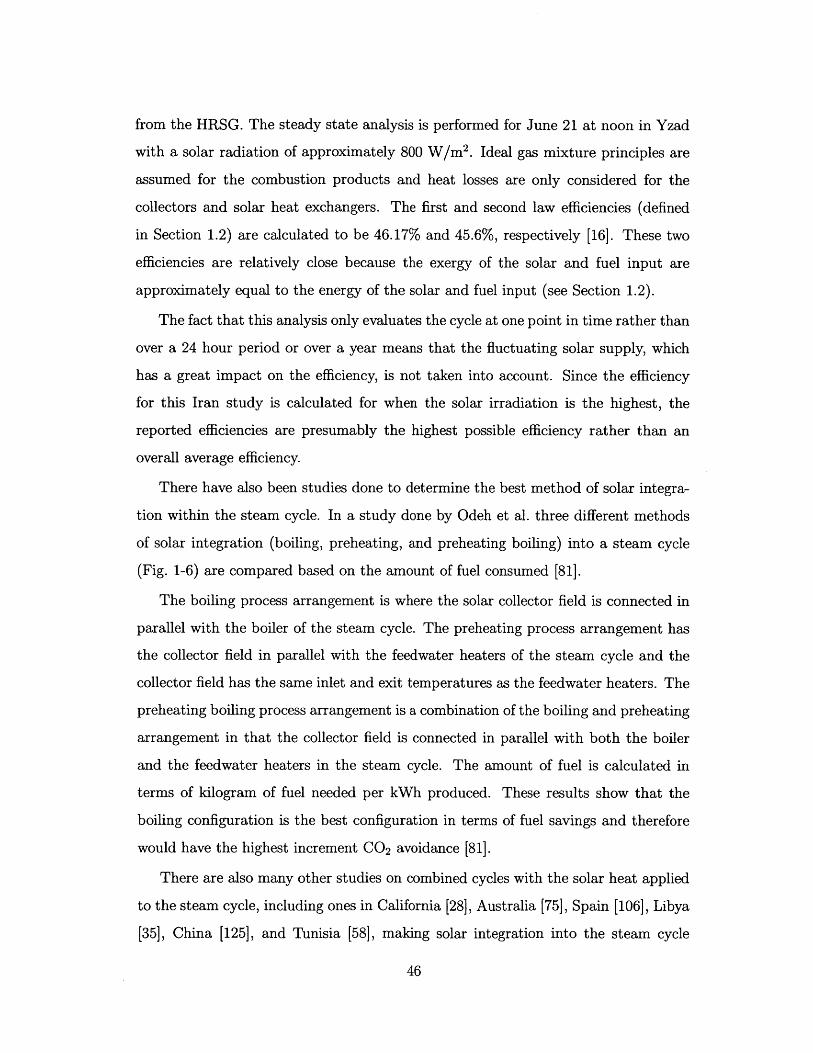
from the HRSG. The steady state analysis is performed for June 21 at noon in Yzad

with a solar radiation of approximately 800 W/m 2 . Ideal gas mixture principles are

assumed for the combustion products and heat losses are only considered for the

collectors and solar heat exchangers. The first and second law efficiencies (defined

in Section 1.2) are calculated to be 46.17% and 45.6%, respectively [16]. These two

efficiencies are relatively close because the exergy of the solar and fuel input are

approximately equal to the energy of the solar and fuel input (see Section 1.2).

The fact that this analysis only evaluates the cycle at one point in time rather than

over a 24 hour period or over a year means that the fluctuating solar supply, which

has a great impact on the efficiency, is not taken into account. Since the efficiency

for this Iran study is calculated for when the solar irradiation is the highest, the

reported efficiencies are presumably the highest possible efficiency rather than an

overall average efficiency.

There have also been studies done to determine the best method of solar integra-

tion within the steam cycle. In a study done by Odeh et al. three different methods

of solar integration (boiling, preheating, and preheating boiling) into a steam cycle

(Fig. 1-6) are compared based on the amount of fuel consumed [81].

The boiling process arrangement is where the solar collector field is connected in

parallel with the boiler of the steam cycle. The preheating process arrangement has

the collector field in parallel with the feedwater heaters of the steam cycle and the

collector field has the same inlet and exit temperatures as the feedwater heaters. The

preheating boiling process arrangement is a combination of the boiling and preheating

arrangement in that the collector field is connected in parallel with both the boiler

and the feedwater heaters in the steam cycle. The amount of fuel is calculated in

terms of kilogram of fuel needed per kWh produced. These results show that the

boiling configuration is the best configuration in terms of fuel savings and therefore

would have the highest increment CO 2 avoidance [81].

There are also many other studies on combined cycles with the solar heat applied

to the steam cycle, including ones in California [28], Australia [75], Spain [106], Libya

[35], China [125], and Tunisia [58], making solar integration into the steam cycle

46

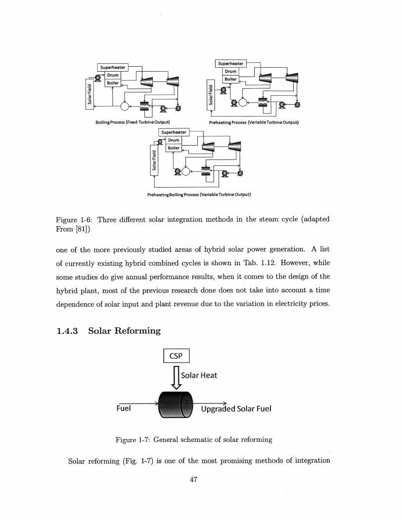
Preheating Process (Variable Turbine Output)

PreheatingBoiling Process (VariableTurbine Output)

Figure 1-6: Three different solar integration methods in the steam cycle (adaptedFrom [81])

one of the more previously studied areas of hybrid solar power generation. A list

of currently existing hybrid combined cycles is shown in Tab. 1.12. However, while

some studies do give annual performance results, when it comes to the design of the

hybrid plant, most of the previous research done does not take into account a time

dependence of solar input and plant revenue due to the variation in electricity prices.

1.4.3 Solar Reforming

Solar Heat

Fuel Upgraded Solar Fuel

Figure 1-7: General schematic of solar reforming

Solar reforming (Fig. 1-7) is one of the most promising methods of integration

47

Boiling Process (Fixed Turbine Output)

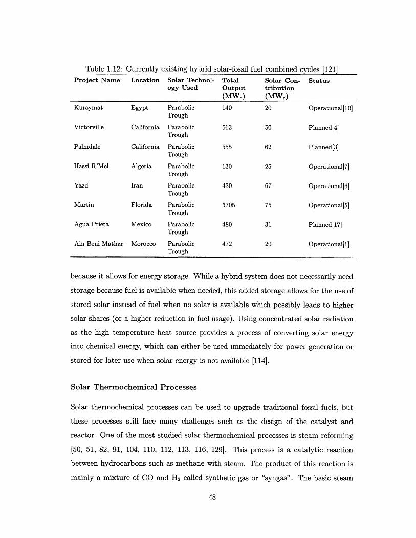
Table 1.12: Currently existing hybrid solar-fossil fuel combined cycles [121]

Project Name Location Solar Technol- Total Solar Con- Statusogy Used Output tribution

(MWe) (MWe)

Kuraymat Egypt Parabolic 140 20 Operational[10]Trough

Victorville California Parabolic 563 50 Planned[4]Trough

Palmdale California Parabolic 555 62 Planned[3]Trough

Hassi R'Mel Algeria Parabolic 130 25 Operational[7]Trough

Yazd Iran Parabolic 430 67 Operational[6]Trough

Martin Florida Parabolic 3705 75 Operational[5]Trough

Agua Prieta Mexico Parabolic 480 31 Planned[17]Trough

Ain Beni Mathar Morocco Parabolic 472 20 Operational[1]Trough

because it allows for energy storage. While a hybrid system does not necessarily need

storage because fuel is available when needed, this added storage allows for the use of

stored solar instead of fuel when no solar is available which possibly leads to higher

solar shares (or a higher reduction in fuel usage). Using concentrated solar radiation

as the high temperature heat source provides a process of converting solar energy

into chemical energy, which can either be used immediately for power generation or

stored for later use when solar energy is not available [114].

Solar Thermochemical Processes

Solar thermochemical processes can be used to upgrade traditional fossil fuels, but

these processes still face many challenges such as the design of the catalyst and

reactor. One of the most studied solar thermochemical processes is steam reforming

[50, 51, 82, 91, 104, 110, 112, 113, 116, 129]. This process is a catalytic reaction

between hydrocarbons such as methane with steam. The product of this reaction is

mainly a mixture of CO and H2 called synthetic gas or "syngas". The basic steam

48

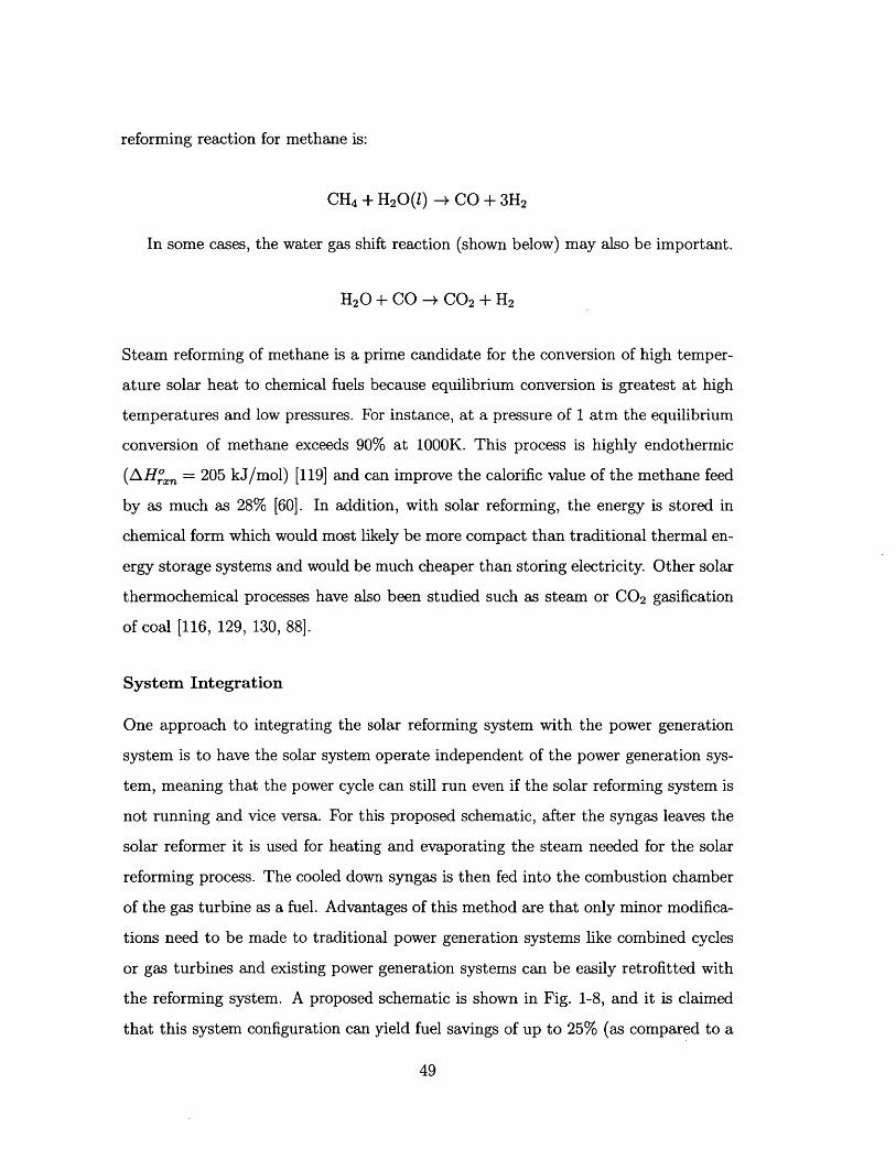
reforming reaction for methane is:

CH 4 + H2 0(l) -+ CO + 3H 2

In some cases, the water gas shift reaction (shown below) may also be important.

H20 + CO - CO2 + H2

Steam reforming of methane is a prime candidate for the conversion of high temper-

ature solar heat to chemical fuels because equilibrium conversion is greatest at high

temperatures and low pressures. For instance, at a pressure of 1 atm the equilibrium

conversion of methane exceeds 90% at 1000K. This process is highly endothermic

(AHr'xn = 205 kJ/mol) [119] and can improve the calorific value of the methane feed

by as much as 28% [60]. In addition, with solar reforming, the energy is stored in

chemical form which would most likely be more compact than traditional thermal en-

ergy storage systems and would be much cheaper than storing electricity. Other solar

thermochemical processes have also been studied such as steam or CO 2 gasification

of coal [116, 129, 130, 88].

System Integration

One approach to integrating the solar reforming system with the power generation

system is to have the solar system operate independent of the power generation sys-

tem, meaning that the power cycle can still run even if the solar reforming system is

not running and vice versa. For this proposed schematic, after the syngas leaves the

solar reformer it is used for heating and evaporating the steam needed for the solar

reforming process. The cooled down syngas is then fed into the combustion chamber

of the gas turbine as a fuel. Advantages of this method are that only minor modifica-

tions need to be made to traditional power generation systems like combined cycles

or gas turbines and existing power generation systems can be easily retrofitted with

the reforming system. A proposed schematic is shown in Fig. 1-8, and it is claimed

that this system configuration can yield fuel savings of up to 25% (as compared to a

49

cycle using methane) [119].

Solar Heat

Syn-Gas

ISuperheater

Preheater

Fuel AirEvaporator

Steam Cycle WS,

Economizer

Water

Figure 1-8: Schematic of solar syngas fired power plant (adapted From [119])

While this integration scheme is promising, some disadvantages include the need

for the storage of gases and the fluctuation of reforming capacity from day to day

unless a thermal storage system is added.

Low/Mid Temperature Cycles

While most hybrid power cycles with solar reforming require high temperatures

from the solar input in order to carry out the reforming reaction, a few cycles have

been proposed that only require low or middle solar input temperatures.

One cycle that uses middle temperature solar heat is the one proposed by Hong

et al. [52] where solar input in the 470-570 K range is used for methanol reforming.

The syngas created from the reforming reaction is then sent to the power cycle (a

combined cycle) as the fuel input. The cycle is simulated in Aspen Plus and the

second law efficiency, solar share, and net incremental solar efficiency are found to be

60.7%, 18%, and 35%, respectively.

Another cycle that uses low/mid temperature solar heat is the SOLRGT cycle

[131]. The SOLRGT cycle uses low/mid temperature solar heat and integrates it with

an intercooled chemically recuperated gas turbine (CRGT) system. A schematic is

shown in Fig. 1-9.

50

w

ReformerRe erator

Eva orator Flue Gas

Solar ite

Economizer W

Figure 1-9: Schematic of SOLRGT cycle (adapted from [131])

A traditional CRGT system uses a HRSG to recover the turbine exhaust gases.

The superheater of the HRSG is replaced with a steam reformer and the reforming

process uses the turbine exhaust as the heat source to produce syngas. In the SOL-

RGT system, low temperature solar heat (470 K-570 K) is used to evaporate water

to generate steam needed for reforming. The steam and fuel are then sent to the

reformer for the production of syngas which is used as the working fluid of the CRGT

system. One of the main advantages of this system is that only low temperature solar

heat is needed whereas with other solar reforming systems high temperature solar

heat is needed which current solar technologies may not be able to meet.

In [131], the turbine is modeled after the cooled turbine model presented in [11]

and the system is simulated using Aspen Plus. The RK-Soave thermodynamic model

is selected for thermal property calculations and the Gibbs Reactor is used to model

the reformer. The Gibbs Reactor determines equilibrium conditions by minimizing

Gibbs free energy. From the simulation, the thermal efficiency is 45.9%, the solar

share is 20.3%, and the incremental solar efficiency is 26.5%. The definitions of these

different metrics are discussed in Section 1.2.

51

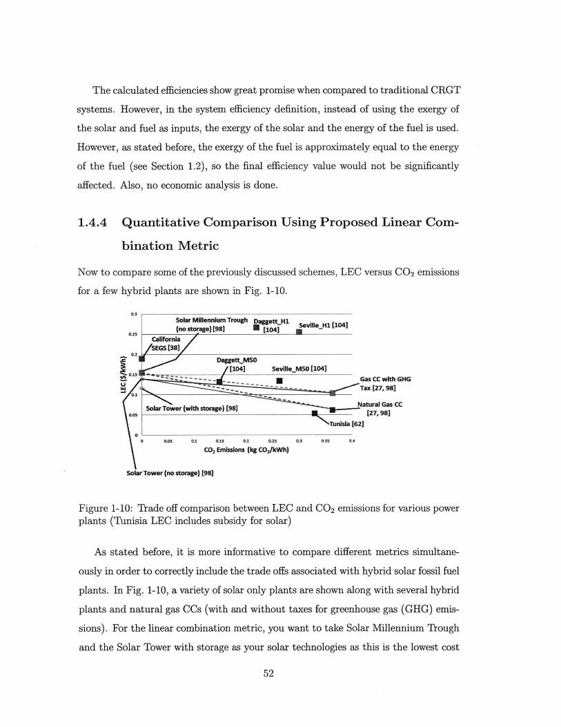
The calculated efficiencies show great promise when compared to traditional CRGT

systems. However, in the system efficiency definition, instead of using the exergy of

the solar and fuel as inputs, the exergy of the solar and the energy of the fuel is used.

However, as stated before, the exergy of the fuel is approximately equal to the energy

of the fuel (see Section 1.2), so the final efficiency value would not be significantly

affected. Also, no economic analysis is done.

1.4.4 Quantitative Comparison Using Proposed Linear Com-

bination Metric

Now to compare some of the previously discussed schemes, LEC versus CO 2 emissions

for a few hybrid plants are shown in Fig. 1-10.

0.3

Solar Millennium Trough Dagett H1 Seville H1[ 1041olar (no storage) [98] 0104

CalifornlaSEGS [318]

0.2Daggett_M50S

As st bo[104] Seviecm [104]plnt-adn a C -(Gas CCwith GHG

141, C k"'_Tax [27, 98]

o Solar T ower (with storage) [9nlg a ai is CC e

0M _' Tunisia [62]

0 0.05 0.2 O.15 0.2 0.25 0.3 0.35 C.4

C02 Emissons (kg CO2/kh)

Sol'ar Tower (no storage) [98]

Figure 1-10: Trade off comparison between LEC and CO2emissions for various powerplants (Tunisia LEC includes subsidy for solar)

As stated before, it is more informative to compare different metrics simultane-

ously in order to correctly include the trade offs associated with hybrid solar fossil fuel

plants. In Fig. 1-10, a variety of solar only plants are shown along with several hybrid

plants and natural gas CCs (with and without taxes for greenhouse gas (GHG) emis-

sions). For the linear combination metric, you want to take Solar Millennium Rough

and the Solar Tower with storage as your solar technologies as this is the lowest cost

52

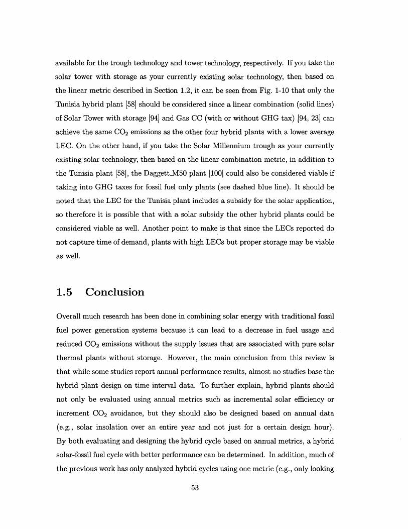
available for the trough technology and tower technology, respectively. If you take the

solar tower with storage as your currently existing solar technology, then based on

the linear metric described in Section 1.2, it can be seen from Fig. 1-10 that only the

Tunisia hybrid plant [58] should be considered since a linear combination (solid lines)

of Solar Tower with storage [94] and Gas CC (with or without GHG tax) [94, 23] can

achieve the same CO2 emissions as the other four hybrid plants with a lower average

LEC. On the other hand, if you take the Solar Millennium trough as your currently

existing solar technology, then based on the linear combination metric, in addition to

the Tunisia plant [58], the DaggettM50 plant [100] could also be considered viable if

taking into GHG taxes for fossil fuel only plants (see dashed blue line). It should be

noted that the LEC for the Tunisia plant includes a subsidy for the solar application,

so therefore it is possible that with a solar subsidy the other hybrid plants could be

considered viable as well. Another point to make is that since the LECs reported do

not capture time of demand, plants with high LECs but proper storage may be viable

as well.

1.5 Conclusion

Overall much research has been done in combining solar energy with traditional fossil

fuel power generation systems because it can lead to a decrease in fuel usage and

reduced CO 2 emissions without the supply issues that are associated with pure solar

thermal plants without storage. However, the main conclusion from this review is

that while some studies report annual performance results, almost no studies base the

hybrid plant design on time interval data. To further explain, hybrid plants should

not only be evaluated using annual metrics such as incremental solar efficiency or

increment CO2 avoidance, but they should also be designed based on annual data

(e.g., solar insolation over an entire year and not just for a certain design hour).

By both evaluating and designing the hybrid cycle based on annual metrics, a hybrid

solar-fossil fuel cycle with better performance can be determined. In addition, much of

the previous work has only analyzed hybrid cycles using one metric (e.g., only looking

53

at efficiency or cost or emissions) or reported various metrics without showing the

tradeoff between them. However, it may be more insightful to evaluate two metrics

simultaneously using the linear combination metric discussed in Section 1.2. This

linear combination metric can be seen as a generalization of the notion of Pareto-

optimal plants (as discussed before in Section 1.2.2) and allows for the comparison

between the proposed hybrid cycle and the current fleet of power plants available.

This comparison gives a more conclusive determination of the viability of the proposed

hybrid cycle.

54

Chapter 2

Hybrid Solar-Fossil Fuel Plant with

Steam Reforming of Methane as

Solar Integration Method

2.1 Introduction

As discussed in Chapter 1 [105], one potential solution to overcoming intermittency

and cost issues associated with solar energy is hybrid concentrated solar-fossil fuel

power generation. Also discussed in Chapter 1 [105] is that existing and proposed

hybrid power generation processes can be grouped into three main areas: solarized gas

turbines, hybrid combined cycles, and solar reforming. Solar reforming, in particular,

is one of the more interesting integration methods because it allows for energy storage

in the form of fuel which can be more compact and cheaper than storing electricity.

While a hybrid system does not necessarily need storage because fuel is available when

needed, this added storage allows for the use of stored solar instead of fuel when no

solar is available which possibly leads to an even higher reduction in fuel usage when

compared to a hybrid cycle with no storage. In addition, the syngas produced by the

solar reforming process is considered a cleaner fuel than natural gas, which means

that by combusting syngas instead of natural gas, there is the potential to reduce

55

emissions when compared to other hybrid cycles that utilize natural gas.

Solar reforming as the integration method for a hybrid cycle is further investigated

based on the aforementioned advantages of the solar reforming integration method

and also because it is the least studied integration option in the literature. The solar

reforming process can, in principle, be integrated with a number of concentrated solar

technologies. In this work, integration with either a parabolic trough or a solar tower

is considered. In the case of the trough reformer, the reformer system is analyzed

on its own and it is demonstrated that it is not a viable option. In the case of the

reforming with a tower, the solar reformer system is also integrated with a combined

cycle in order to optimize the design and operation of a hybrid solar-fossil fuel plant

using solar reforming.

2.2 Parabolic Though Reforming

First, the integration of solar reforming with a parabolic trough will be discussed.

2.2.1 Model Description

The trough model is based on the Sandia model [37]. The trough model is created

in Aspen Custom Modeler@ and then implemented with a steam reforming model in

Aspen Plus@.

Parabolic Trough Model

As discussed in Chapter 1 [105], a trough uses a single-axis tracking curved mir-

ror system to concentrate solar radiation onto a receiver pipe through which a heat

transfer fluid (HTF) flows. Herein, the trough is represented by a steel pipe with

a glass cover. Vacuum conditions are assumed between the glass cover and pipe as

shown in Fig. 2-1. The model takes as inputs the solar DNI, area of solar collection,

environment parameters (i.e., temperature, wind speed, etc.), HTF parameters (in-

let temperature and pressure, flow rate, density, heat capacity, and viscosity), and

trough parameters (length, material properties, diameter of pipe, etc.) and outputs

56

the outlet temperature and pressure of the HTF. In order to calculate the outputs,

the model first calculates the optical efficiency to determine the amount of energy

actually absorbed by the pipe. Then the model discretizes the pipe into equally sized

elements and a steady state energy balance is performed on each element (taking into

account convection and conduction) in order to determine the outlet temperature of

each element. The pressure drop across each element is then also calculated.

Steel Pipe

TB

g

Figure 2-1: Cross-section of Parabolic Trough Receiver

The optical efficiency is calculated using several optical parameters and the inci-

dence angle of the sun (0). The incidence angle is defined as the angle between the

sun's rays and the normal line of the parabolic mirror. The formula for the optical

efficiency is as follows:

7io = e1 2 es e e5 e6 Pci K T

where ei, e2 , e3 , e4, e5 , and e6 are various optical parameters defined in Tab. 2.1,

Pc is the clean mirror reflectance, r is the transmittance of the glass cover, and K

is the incident angle modifier. The incident angle modifier K is calculated using the

57

Glass Cover

following equation:

K = cos(G) + 0.0008840 - 0.0000536962

Table 2.1: Optical parameters for calculation of optical efficiency [37]Parameter Description Value

el Shadowing parameter .974

e2 Tracking error .994

e3 Geometry error .98

e4 Dirt on mirror parameter reflectivity of clear mirror/pd

e5 Dirt on receiver parameter 1-e4

e6 Random error .96

peC Reflectivity of clear mirror .88

Pd Clean mirror reflectance .935T Transmittance of glass cover .935

The amount of energy absorbed by the pipe is then equal to:

Qabs =qA ar7o

where q is the DNI, A is the total area of collection, a is the absorptance of the

pipe, and ro is the optical efficiency calculated. Once the optical losses are taken into

account, the energy balance for each individual element is performed based on the

thermal resistance network shown in Fig. 2-2. In the resistance network, TB is the

bulk temperature of the HTF, Tpi is inner wall temperature of the pipe, Tp,0 is outer

wall temperature of the pipe, Tgi is the inner wall temperature of the glass cover,

Tg,o is the outer wall temperature of the glass cover, and Tamb is the environment

temperature. The temperatures are also shown schematically in Fig. 2-1.

Conv Cond Conv Cond ConvTBV/\\rTA \/\/\reT,,O* \/\/\r*Tg.N\/AA\/re Tgo*N\/V/\rTamb

Figure 2-2: Trough Model Resistor Network

The resistances in the network are calculated using standard methods. The Nus-

58

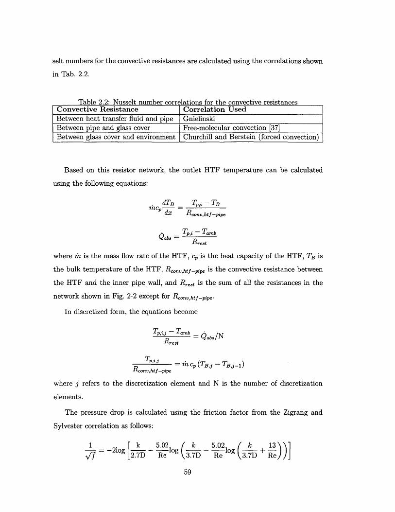
selt numbers for the convective resistances are calculated using the correlations shown

in Tab. 2.2.

Table 2.2: Nusselt number correlations for the convective resistancesConvective Resistance Correlation UsedBetween heat transfer fluid and pipe GnielinskiBetween pipe and glass cover Free-molecular convection [37]Between glass cover and environment Churchill and Berstein (forced convection)

Based on this resistor network, the outlet HTF temperature can be calculated

using the following equations:

dTB Tp,i -TBmncd =

dx Rconv,htf -,1,e

T,, - Tamb

Qabs = Rrest

where rh is the mass flow rate of the HTF, c, is the heat capacity of the HTF, TB is

the bulk temperature of the HTF, Rcoo,htf _pie is the convective resistance between

the HTF and the inner pipe wall, and Rrest is the sum of all the resistances in the

network shown in Fig. 2-2 except for Rconovatf -,ie

In discretized form, the equations become

T,,,Tamb Qabs/NRrest =QbI

T,,_ = rh c, (TB,j - TBJ1)Rconv,ht f -pipe

where j refers to the discretization element and N is the number of discretization

elements.

The pressure drop is calculated using the friction factor from the Zigrang and

Sylvester correlation as follows:

1 =k 5.02 ( k 5.02 ( k 13N j= -2log [.D- log elog + Re--/

vf 2.7D) Re 3.7D Re 3.7D Re

59

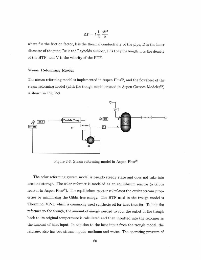
AP = f vD 2

where f is the friction factor, k is the thermal conductivity of the pipe, D is the inner

diameter of the pipe, Re is the Reynolds number, L is the pipe length, p is the density

of the HTF, and V is the velocity of the HTF.

Steam Reforming Model

The steam reforming model is implemented in Aspen Plus®, and the flowsheet of the

steam reforming model (with the trough model created in Aspen Custom Modeler®)

is shown in Fig. 2-3.

e"

KffNParabolic Trough

B3

Figure 2-3: Steam reforming model in Aspen Plus®

The solar reforming system model is pseudo steady state and does not take into

account storage. The solar reformer is modeled as an equilibrium reactor (a Gibbs

reactor in Aspen Plus®). The equilibrium reactor calculates the outlet stream prop-

erties by minimizing the Gibbs free energy. The HTF used in the trough model is

Therminol VP-1, which is commonly used synthetic oil for heat transfer. To link the

reformer to the trough, the amount of energy needed to cool the outlet of the trough

back to its original temperature is calculated and then inputted into the reformer as

the amount of heat input. In addition to the heat input from the trough model, the

reformer also has two stream inputs: methane and water. The operating pressure of

60

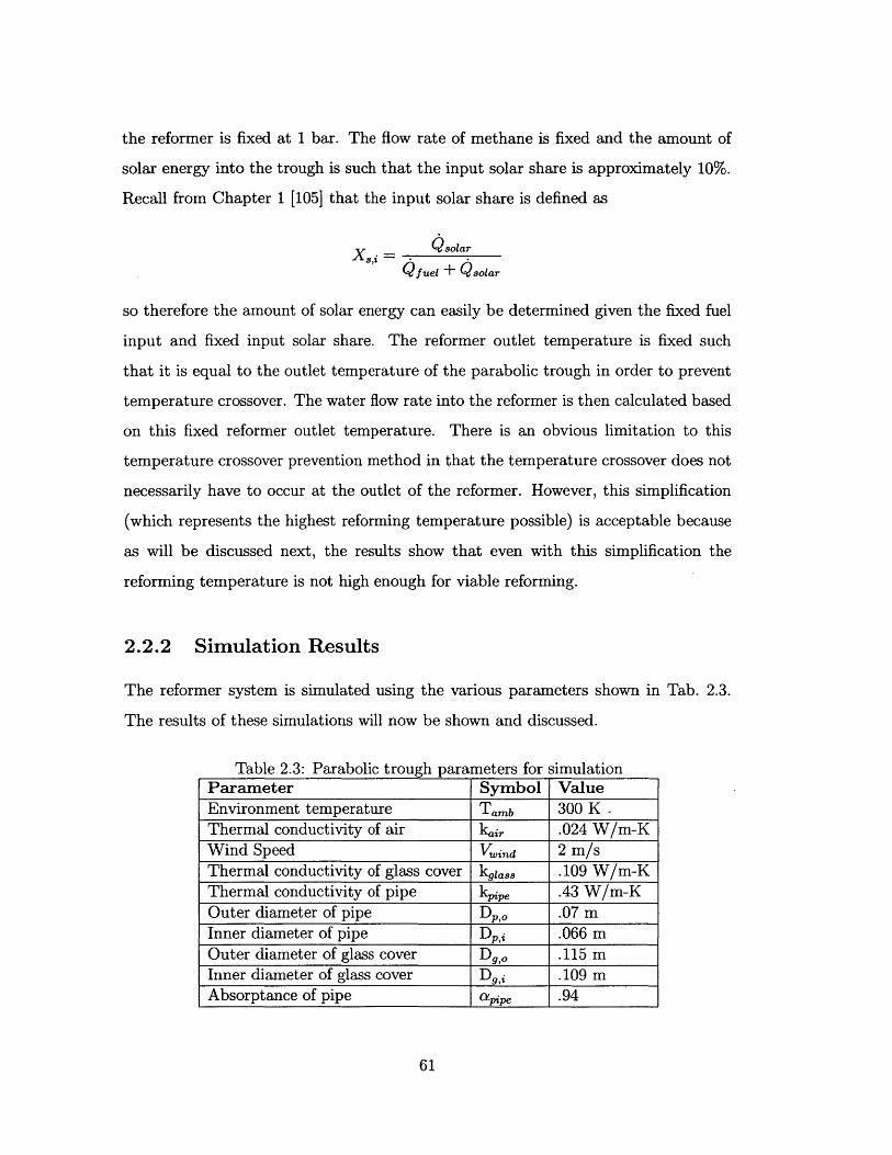
the reformer is fixed at 1 bar. The flow rate of methane is fixed and the amount of

solar energy into the trough is such that the input solar share is approximately 10%.

Recall from Chapter 1 [105] that the input solar share is defined as

= .Qsoar

Qiuel + Qsolar

so therefore the amount of solar energy can easily be determined given the fixed fuel

input and fixed input solar share. The reformer outlet temperature is fixed such

that it is equal to the outlet temperature of the parabolic trough in order to prevent

temperature crossover. The water flow rate into the reformer is then calculated based

on this fixed reformer outlet temperature. There is an obvious limitation to this

temperature crossover prevention method in that the temperature crossover does not

necessarily have to occur at the outlet of the reformer. However, this simplification

(which represents the highest reforming temperature possible) is acceptable because

as will be discussed next, the results show that even with this simplification the

reforming temperature is not high enough for viable reforming.

2.2.2 Simulation Results

The reformer system is simulated using the various parameters shown in Tab. 2.3.

The results of these simulations will now be shown and discussed.

Table 2.3: Parabolic trough parameters for simulationParameter Symbol ValueEnvironment temperature Tamb 300 KThermal conductivity of air kair .024 W/m-KWind Speed Vwind 2 m/sThermal conductivity of glass cover kglas, .109 W/m-KThermal conductivity of pipe kppe .43 W/m-KOuter diameter of pipe D,, 0 .07 mInner diameter of pipe D,, .066 mOuter diameter of glass cover D,,o .115 mInner diameter of glass cover Dgi .109 mAbsorptance of pipe api, .94

61

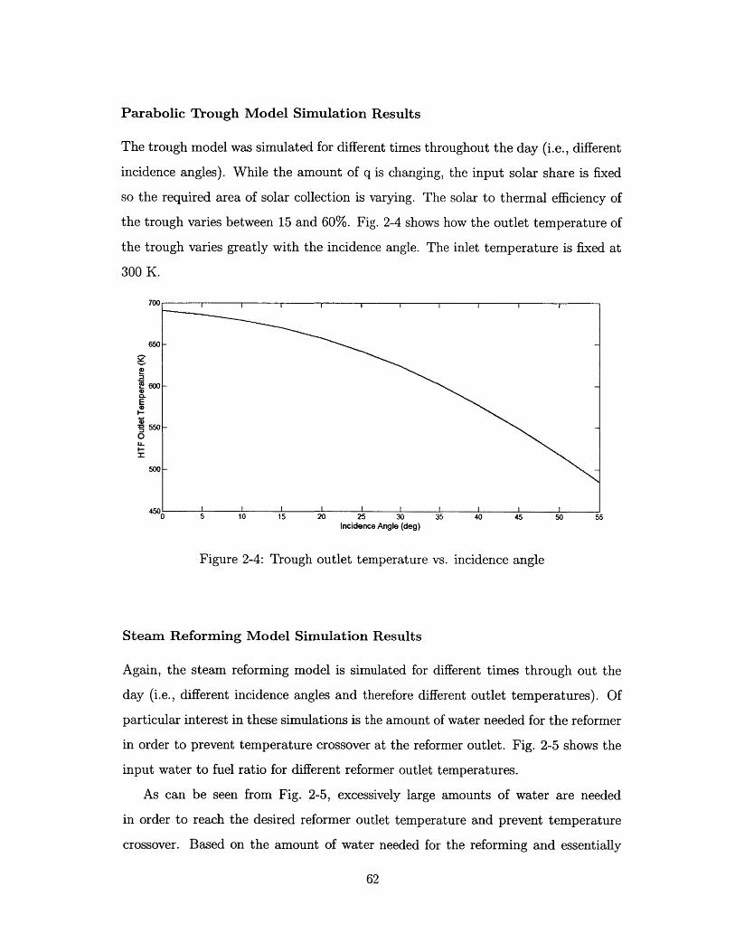
Parabolic Trough Model Simulation Results

The trough model was simulated for different times throughout the day (i.e., different

incidence angles). While the amount of q is changing, the input solar share is fixed

so the required area of solar collection is varying. The solar to thermal efficiency of

the trough varies between 15 and 60%. Fig. 2-4 shows how the outlet temperature of

the trough varies greatly with the incidence angle. The inlet temperature is fixed at

300 K.

650

E

0

LL

60W

550

500

0 5 10 15 20 25 30Incidence Angle (deg)

35 40 45 50 55

Figure 2-4: Trough outlet temperature vs. incidence angle

Steam Reforming Model Simulation Results

Again, the steam reforming model is simulated for different times through out the

day (i.e., different incidence angles and therefore different outlet temperatures). Of

particular interest in these simulations is the amount of water needed for the reformer

in order to prevent temperature crossover at the reformer outlet. Fig. 2-5 shows the

input water to fuel ratio for different reformer outlet temperatures.

As can be seen from Fig. 2-5, excessively large amounts of water are needed

in order to reach the desired reformer outlet temperature and prevent temperature

crossover. Based on the amount of water needed for the reforming and essentially

62

I g I I I I I I

4000 -

03500-

-i

.2 3000-0

CL 2500-

2000-

150I II I I 70050500 550 600 65071

Reformer Outlet Temperature (K)

Figure 2-5: Input water to fuel ratio for various reformer outlet temperatures

full conversion of methane, the outlet mole fraction of hydrogen and carbon dioxide

are, as expected, quite low with the mole fraction carbon monoxide negligible. The

mole fractions of the hydrogen and carbon dioxide only change with differing reformer

temperature because of the different amounts of water needed.

Based on the simulations results, a first law analysis is performed to determine the

amount of energy needed for the three main processes occurring in the reformer: the

actual reforming, the heating of the methane to the reformer operating temperature,

and the heating/evaporating of the water. Tab. 2.4 shows the percentage of the

reformer heat input used for each process. From Tab. 2.4, it can be seen that most of

the energy input into the reformer is being using for the heating/evaporating of the

water, and the reformer acts primarily as a steam generator.

In essence, parabolic troughs are not suitable for solar steam reforming of methane

because of the relatively low operating temperatures. Substantially higher temper-

atures are required to reduce the water amount. Therefore, the parabolic trough is

more ideally suited for a lower temperature integration method (e.g., in a steam cycle

as discussed in Chapter 1 [105]), and for solar reforming, a technology that can reach

higher operating temperatures (e.g., tower) would be more desirable. It should be

also noted that troughs could be used with solar reforming processes that do not

63

Table 2.4: Energy breakdown for different processes in reformerReformer % of En- % of En- % of Energy -

Tempera- ergy - ergy - Heat- Reformingture (K) Heating ing/Evaporating

Methane Water485 7.75e-3 99.8 .179518 7.70e-3 99.8 .150549 7.67e-3 99.9 .129577 7.64e-3 99.9 .114602 7.61e-3 99.9 .103624 7.59e-3 99.9 .095642 7.54e-3 99.9 .089658 7.53e-3 99.9 .084670 7.50e-3 99.9 .080679 7.46e-3 99.9 .078686 7.46e-3 99.9 .076691 7.47e-3 99.9 .075

require as high of temperature such as methanol decomposition

assisted chemically recuperated gas turbine [131].

[52] or using a solar

2.3 Tower Reforming Cycle

Since, as seen with the trough reforming simulations, the reforming process requires

a higher operating temperature than the troughs are able to provide, the reformer is

now integrated with a solar tower (which can reach higher temperatures as discussed

in Chapter 1 [105]) and the tower reformer is then integrated with a combined cycle.

This combined cycle integrated with a tower reformer is based on the solar reforming

hybrid cycle proposed in [119], however, the analysis here is more in depth in that an

optimization of both design and operation is performed for the hybrid cycle, fluctua-

tion of the solar supply is accounted for in both design and operation, and off-design

conditions are also considered.

2.3.1 Hybrid Cycle Model Description

The hybrid power cycle flowsheet is shown in Fig. 2-6 and modeled entirely in Aspen

Plus@. It is a standard combined cycle with a triple pressure Heat Recovery Steam

64

Water

Air

Tower HSG-CReformer

-- - -- -- -- -

Methane

Figure 2-6: Power cycle flowsheet

Generator (HRSG). The solar technology used in this hybrid cycle is a central receiver

reformer. The water needed for reforming is first pumped to the pressure of the

combustor and then preheated in the HRSG before being mixed with the methane,

which is already compressed to the appropriate pressure. The methane and water

mixture is then evaporated using the tower reformer outlet in order to turn the water

into steam before being sent to the tower reformer. All the syngas created by the

reformer is then sent to the gas turbine cycle as the working fluid. The compressed air

is sent to the combustor, and the combustion is assumed to be complete and adiabatic.

It should be noted that in actual practice, only a portion of the air would be sent

to the combustor and then the remaining air would be mixed with the outlet of the

combustor for temperature control. However, since the combustor herein is modeled

as a black box, thermodynamically both methods will yield the same results. The flue

gas is then used in the HRSG of the steam cycle. The steam cycle is designed such that

the expanded steam from the high pressure turbine is mixed with the intermediate

pressure superheated steam before being sent to the intermediate pressure turbine.

The same is also true for the low pressure turbine in that the expanded steam from

65

the intermediate pressure turbine is also mixed with the low pressure steam from the

HRSG before being expanded through the low pressure turbine. The outlet of the low

pressure steam is split between the deaerator and condenser before being sent back

to the HRSG. The pinch values within each section of the HRSG are fixed (discussed

in more detail later) and for the compressors and turbines, an isentropic efficiency is

utilized to calculate the outlet conditions. The methane is assumed to be an ideal gas

and all pressure drops are neglected except for the pressure drop across the HRSG

(Section 2.3.2).

For the power cycle model, solar energy is only utilized if there is an input solar

share of at least 10%. When there is not enough solar energy, the solar technology

is bypassed (i.e., no reforming), and the methane is sent directly to the combustor

and no water is needed for reforming. The model is also pseudo steady state and no

storage is considered.

Tower Reformer Model

The reformer model is created in Aspen custom modeler and integrates the reformer

reactor with the solar receiver. The receiver reactor is assumed to be cylindrical

in shape, and the model takes into account optical, radiation, and convection heat

losses. The pressure drop across the tower reformer is neglected, and the operating

temperature is assumed to be equal to the reforming temperature. An example trend

of the variation of the reforming temperature throughout the day is shown in Fig. 2-

7. As expected, the more solar energy available (i.e., peak solar energy available at

approximately hour 12) the higher the reformer temperature.

The radiation losses are calculated using the following equation [102]:

Qrad = AEef5T 4

where A is the area of the receiver, eff is the effective emissivity of the receiver, and

T is the operating temperature of the receiver reactor. The convection heat losses are

66

1LuuI I I I I 1

1150-

0 0 1 0

a 950 /

Hour

Figure 2-7: Reformer Temperature Variation (May 1)

calculated using the following equations [102]:

Q con, Ah(T - Tam,,b)

h = 0.557X10-6 T - Tamb 0.25 [W/m 2-K]

where the convection heat transfer coefficient (h) is calculated using the Bejan corre-

lation for vertical chamber with natural convection and H is the height of the receiver.

The radiation and convection heat loss variation throughout the day is shown in Fig-

ure 2-8. As can be seen from Fig. 2-7 and Fig. 2-8, the higher heat losses correspond

to the higher reforming temperatures. However, it should also be noted that heat

losses are rather insignificant compared to the heat transfer rate to the receiver with

radiation losses accounting for less than 6% of the heat transfer rate to the receiver

and the convection losses accounting for less than 1% of the heat transfer rate to the

receiver.

The optical efficiency is calculated from the model presented in [79]. This model

is used because it gives a time variable optical efficiency, which is more accurate than

a time-invariant optical efficiency. This model also uses a biomemtic heliostat pattern

67

240 I

200r -

180- -

160 -

> 14"C0

8 9 10 11 12 13 14 15 18Hour

I.589 10 11 12 13 14 15 16Hour

Figure 2-8: Convection Heat Loss (Top in W) and Radiation Heat Loss (Bottom inMW) Variation (May 1)

which leads to less land area and higher optical efficiency than traditional heliostat

field designs.

The reformer is modeled such that both steam reforming of methane and the water

gas shift reaction are taken into account. The possible products are fixed to CH 4 ,

H20, H2 , CO 2 , and CO, and the reformer model is based on the stoichiometric method

for equilibrium. The temperature and outlet composition is calculated using the Law

of Mass Action, standard Gibbs free energy of reaction, and an energy balance as

shown below:e-A G(T) P ^'s

exp RT PO

7lopt~solar - Qrad - = on i'outhi'out - tii,inhi,in

where i refers to the specific species, j refers to the specific reaction (stoichiometric),

P is the pressure of the reformer, T is the reforming temperature, vij, is the stoi-

chiometric coefficient of species i in reaction j, Xjj is the mole fraction of species

i in reaction j, A0, G is the Gibbs free energy of reaction at standard pressure of

reaction j, 7,tp is the optical efficiency, Qsolar is the total solar input (DNI multiplied

68

by heliostat area), ni is the molar flow rate of species i, and h (in/out) is the molar

enthalpy.

DNI Data

The solar DNI data used in the power cycle model is obtained from the weather

station at King Fahd University of Petroleum and Minerals (KFUPM) in Dhaharan,

Saudi Arabia. The DNI is given in an hourly interval for an entire year. The DNI

data is from the year 2008. Plots of the DNI for the entire day for different times of

the year are shown in Fig. 2-9.

o000 --

- -Jan 1800 - ' , -- Mar 1

7006- -+- May 1700 A -Jul

+ Sept 1

500H

400-1

300 /'''

200 /

100-'"~''

05 10 12025

Hour

Figure 2-9: DNI trends throughout the day for various days in the year

Note that the DNI is not perfectly symmetric around hour 12 (as you would

expect for perfect weather situations). Also, since perfect weather is not assumed,

there are anomalies within a day where the DNI values does to follow the expected

trend. An example of these anomalies can be seen in Fig. 2-9 with the DNI plot for

November 1. On November 1, the DNI value unexpectedly dips at noon rather than

reaching a peak indicating cloud coverage or other weather phenomena. In addition

to anomalies within a day, there can also be entire days where the solar DNI is much

less than ideal. For example, in Fig. 2-10, the DNI values for January 14 are overall

significantly lower than both the day before and after it.

69

.300 -

200-

100 a" a

0 5 10 15 20 25Hour

Figure 2-10: Example of a "cloudy" day: DNI values much less than ideal

Essentially, by not assuming perfect weather, the simulation also captures possible

random weather anomalies that would affect whether or not there is enough solar

energy available to be used with the hybrid power cycle.

2.3.2 Optimization

After the hybrid cycle model is created, its design and operation is optimized using

the built in Aspen Plus@ optimizer, which utilizes an SQP method of optimization.

The objective function is to maximize the work output for a fixed fuel input and fixed

heliostat area (in essence maximizing the first law efficiency) over an entire year (i.e.,

taking into account fluctuating solar energy supply).

2-Step Optimization Process

Due to the limitations of the Aspen optimizer, the optimization over the entire year

is performed using a two step process. The first step is to optimize the cycle over

the entire year allowing for both design and operational variables to vary. In reality,

only the operational variables would be able to vary throughout the entire year, so

this first optimization step, in essence, represents an upper bound on the performance

of the cycle (assuming that the global optimum is found). The second step of the

optimization process is then to run the optimization again but this time only allowing

70

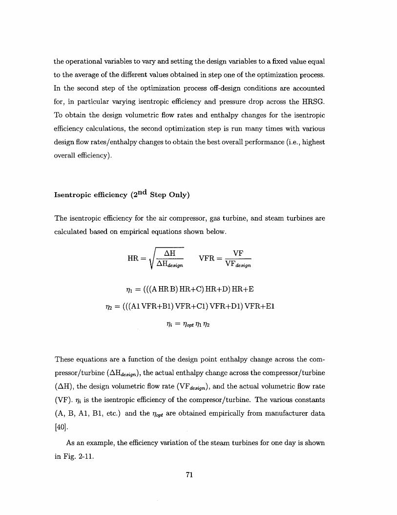
the operational variables to vary and setting the design variables to a fixed value equal

to the average of the different values obtained in step one of the optimization process.

In the second step of the optimization process off-design conditions are accounted

for, in particular varying isentropic efficiency and pressure drop across the HRSG.

To obtain the design volumetric flow rates and enthalpy changes for the isentropic

efficiency calculations, the second optimization step is run many times with various

design flow rates/enthalpy changes to obtain the best overall performance (i.e., highest

overall efficiency).

Isentropic efficiency (2 nd Step Only)

The isentropic efficiency for the air compressor, gas turbine, and steam turbines are

calculated based on empirical equations shown below.

HR = AH VFR VFLAHdesign VFdesign

71 = (((A HR B) HR+C) HR+D) HR+E

?72 = (((Al VFR+B1) VFR+C1) VFR+D1) VFR+E1

77i = 77opt 7 17 T2

These equations are a function of the design point enthalpy change across the com-

pressor/turbine (AHde,,ign), the actual enthalpy change across the compressor/turbine

(AH), the design volumetric flow rate (VFesign), and the actual volumetric flow rate

(VF). qj is the isentropic efficiency of the compresor/turbine. The various constants

(A, B, Al, B1, etc.) and the ,,t are obtained empirically from manufacturer data

[40].

As an example, the efficiency variation of the steam turbines for one day is shown

in Fig. 2-11.

71

80r -- Intermediate Pressure Turbine--- Low Pressure Turbine

79 --

-78 -

76

75-/

741III8 9 10 11 12 13 14 15 16

Hour

Figure 2-11: Isentropic Efficiency Variation of Steam Turbines for May 1 "

HRSG Pressure Drop (2 nd Step Only)

The pressure drop is calculated by first calculating the friction factor using the Moody

equation shown below:

/ 106 \f = .0055 1+ 2x104-" +

D Re

Then the pressure drop is calculated as follows:

AP f L pV 2

D 2

Optimization Variables

The optimization (both design and operational) variables and their values/ranges are

shown in Tab. 2.5.

As stated previously, the design variables are fixed during the second step of the

optimization. The values for these design variables are determined by averaging over

the entire year for the values obtained from the first step optimization.

72

I I I I I I Turbine

-- *-- High Pressure Turbine-

MI

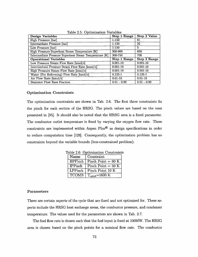
Table 2.5: Optimization VariablesDesign Variables Step 1 Range Step 2 ValueHigh Pressure [bar] 1-150 81Intermediate Pressure [bar] 1-150 25Low Pressure [bar] 1-150 5High Pressure Superheat Steam Temperature [K] 500-900 850Intermediate Pressure Superheat Steam Temperature [K] 300-750 700Operational Variables Step 1 Range Step 2 Range

Low Pressure Steam Flow Rate [kmol/s] 0.001-10 0.001-10Intermediate Pressure Steam Flow Rate [kmol/s] 0.001-10 0.001-10High Pressure Steam Flow Rate [kmol/s] 0.001-10 0.001-10Water (For Reforming) Flow Rate [kmol/s] 0.125-1 0.125-1Air Flow Rate (kmol/s] 0.01-10 0.01-10Dearator Flow Rate Fraction 0.01 - 0.99 0.01 - 0.99

Optimization Constraints

The optimization constraints are shown in Tab. 2.6. The first three constraints fix

the pinch for each section of the HRSG. The pinch values are based on the ones

presented in [95]. It should also be noted that the HRSG area is a fixed parameter.

The combustor outlet temperature is fixed by varying the oxygen flow rate. These

constraints are implemented within Aspen Plus@ as design specifications in order

to reduce computation time [128]. Consequently, the optimization problem has no

constraints beyond the variable bounds (box-constrained problem).

Table 2.6: Optimization ConstraintsName ConstraintHPPinch Pinch Point = 60 KIPPinch Pinch Point = 50 KLPPinch Pinch Point 10 KTCOMB Tcomb=1600 K

Parameters

There are certain aspects of the cycle that are fixed and not optimized for. These as-

pects include the HRSG heat exchange areas, the combustor pressure, and condenser

temperature. The values used for the parameters are shown in Tab. 2.7.

The fuel flow rate is chosen such that the fuel input is fixed at 100MW. The HRSG

area is chosen based on the pinch points for a nominal flow rate. The combustor

73

Table 2.7: Optimization ParametersParameter ValueFuel Flow Rate 0.125 kmol/sReformer Diameter 5 mReformer Height 10 mSolar Field Area 50,000 m 2

HRSG Area 923 m2

Combustor Pressure 30 barCondenser Temperature 310 K

pressure and condenser temperature are chosen based on typical plant operation [27].

The solar field area is chosen such that the maximum input solar share over the entire

year is 34.4%. Similar to when determining the amount of solar energy for the trough

reforming, the following formula is again used to calculate the required area:

23tfu R usolar

2.3.3 Optimization Results

Table 2.8: Key Optimization ResultsMetric ValueAnnual Cycle Efficiency 47.59%Annual Incremental Solar Efficiency 26.11%Maximum Input Solar Share 34.40%Maximum Output Solar Share 20.52%Annual Input Solar Share 9.58%Annual Output Solar Share 5.39%Annual CO 2 Emissions 0.386 kg/kWh

First to summarize the optimization results, Tab. 2.8 shows the values for various

metrics discussed in Chapter 1 [105].All the annual metrics include the time when

there is no solar available. The typical solar share variation throughout the day is

shown in Figure 2-12. It should be noted that only hours during the day in which

the solar is actually used within the hybrid cycle are shown.

As expected, the solar shares - both input and output - follow the trend of the

solar irradiance (i.e., the more solar energy available the higher the input and output

74

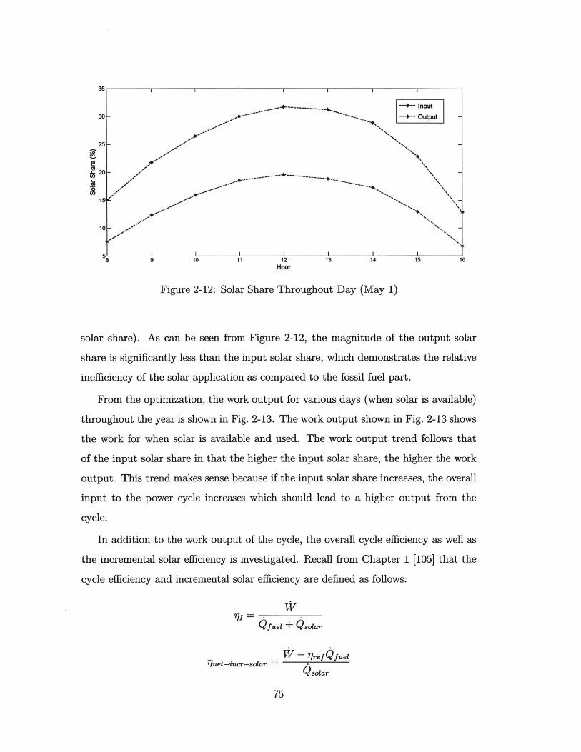
0

0

Hour

Figure 2-12: Solar Share Throughout Day (May 1)

solar share). As can be seen from Figure 2-12, the magnitude of the output solar

share is significantly less than the input solar share, which demonstrates the relative

inefficiency of the solar application as compared to the fossil fuel part.

From the optimization, the work output for various days (when solar is available)

throughout the year is shown in Fig. 2-13. The work output shown in Fig. 2-13 shows

the work for when solar is available and used. The work output trend follows that

of the input solar share in that the higher the input solar share, the higher the work

output. This trend makes sense because if the input solar share increases, the overall

input to the power cycle increases which should lead to a higher output from the

cycle.

In addition to the work output of the cycle, the overall cycle efficiency as well as

the incremental solar efficiency is investigated. Recall from Chapter 1 [105] that the

cycle efficiency and incremental solar efficiency are defined as follows:

Qfuel + Qsolar

~_ W-iref Qfuel1 net-incr-solar -

solar

75

~56 -,.

0 55-

~54 '

51/'

518 9 10 11 12 13 14 15 16 17

Hour

Figure 2-13: Work Output Throughout Entire Year

In this analysis, the reference cycle efficiency is obtained by optimizing the cycle

flowsheet without the solar reformer. From this optimization the reference cycle

efficiency is set at 48.56%. The comparison of these two efficiencies is shown for a

particular day in Fig. 2-14.

50

40

35

w30

25

9 10 11 12Hour

13 14 15 16

Figure 2-14: Comparison of Cycle and Incremental Solar Efficiency for May 1

For the overall cycle efficiency, it decreases as the input solar share increases. This

trend is because the solar part of the hybrid cycle is relatively inefficient when com-

paring to the fossil fuel part. Therefore, when the solar share is increased, the solar

76

--- Cycle Efficiency-.. Incremental Solar Efficiency -

--- ------------

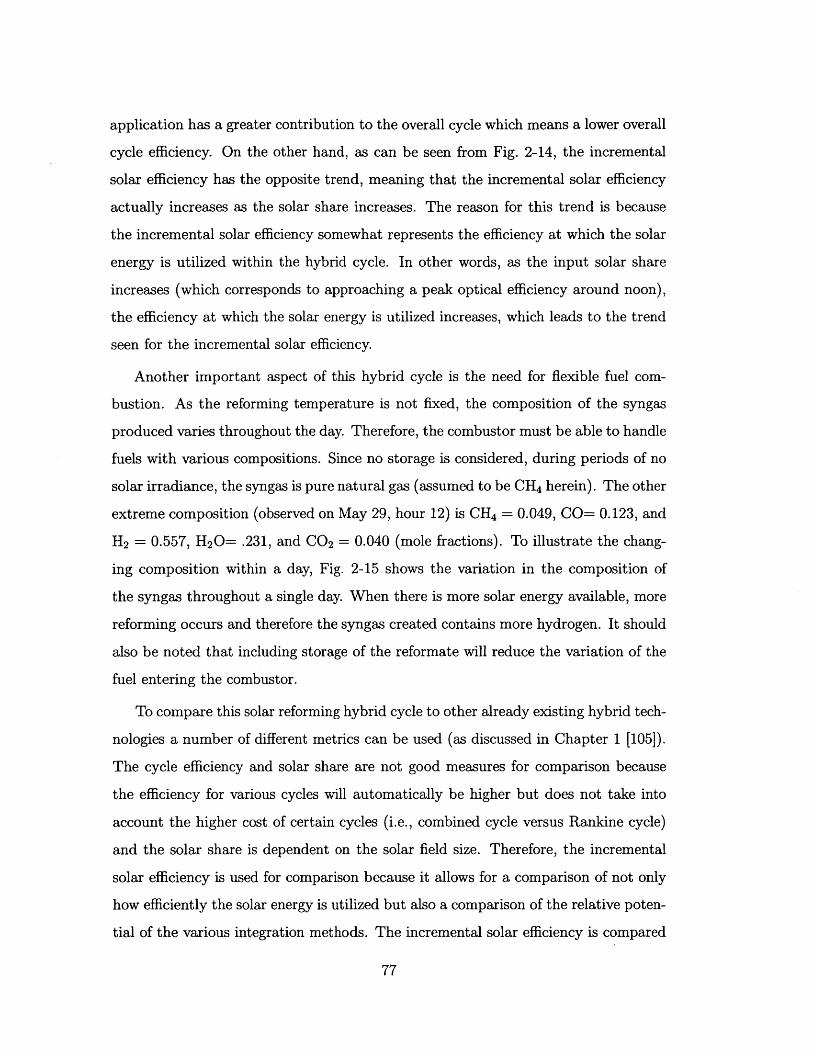
application has a greater contribution to the overall cycle which means a lower overall

cycle efficiency. On the other hand, as can be seen from Fig. 2-14, the incremental

solar efficiency has the opposite trend, meaning that the incremental solar efficiency

actually increases as the solar share increases. The reason for this trend is because

the incremental solar efficiency somewhat represents the efficiency at which the solar

energy is utilized within the hybrid cycle. In other words, as the input solar share

increases (which corresponds to approaching a peak optical efficiency around noon),

the efficiency at which the solar energy is utilized increases, which leads to the trend

seen for the incremental solar efficiency.

Another important aspect of this hybrid cycle is the need for flexible fuel com-

bustion. As the reforming temperature is not fixed, the composition of the syngas

produced varies throughout the day. Therefore, the combustor must be able to handle

fuels with various compositions. Since no storage is considered, during periods of no

solar irradiance, the syngas is pure natural gas (assumed to be CH 4 herein). The other

extreme composition (observed on May 29, hour 12) is CH 4 = 0.049, CO= 0.123, and

H2 = 0.557, H2 0= .231, and CO2 = 0.040 (mole fractions). To illustrate the chang-

ing composition within a day, Fig. 2-15 shows the variation in the composition of

the syngas throughout a single day. When there is more solar energy available, more

reforming occurs and therefore the syngas created contains more hydrogen. It should

also be noted that including storage of the reformate will reduce the variation of the

fuel entering the combustor.

To compare this solar reforming hybrid cycle to other already existing hybrid tech-

nologies a number of different metrics can be used (as discussed in Chapter 1 [105]).

The cycle efficiency and solar share are not good measures for comparison because

the efficiency for various cycles will automatically be higher but does not take into

account the higher cost of certain cycles (i.e., combined cycle versus Rankine cycle)

and the solar share is dependent on the solar field size. Therefore, the incremental

solar efficiency is used for comparison because it allows for a comparison of not only

how efficiently the solar energy is utilized but also a comparison of the relative poten-

tial of the various integration methods. The incremental solar efficiency is compared

77

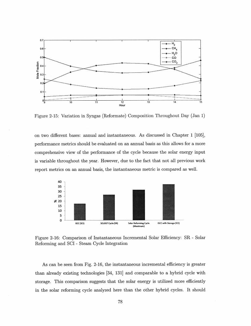
0.7 1 1 1---- H2

0.6- ----- CH4---- H2O0 -*-. 2Co

0.5- CO-r- CO2

-------------------------------------------0f OA -

0.1-

--

-9 10 11 12 13 14 15Hour

Figure 2-15: Variation in Syngas (Reformate) Composition Throughout Day (Jan 1)

on two different bases: annual and instantaneous. As discussed in Chapter 1 [105],

performance metrics should be evaluated on an annual basis as this allows for a more

comprehensive view of the performance of the cycle because the solar energy input

is variable throughout the year. However, due to the fact that not all previous work

report metrics on an annual basis, the instantaneous metric is compared as well.

40

35

30 -25

20

ISCC (SCI) SOLRGT Cycle (SR) Solar ReforrIng Cycle ISCC wIth Storage (SCI)(Maxinurn)

Figure 2-16: Comparison of Instantaneous Incremental Solar Efficiency: SR - Solar

Reforming and SCI - Steam Cycle Integration

As can be seen from Fig. 2-16, the instantaneous incremental efficiency is greater

than already existing technologies [34, 131] and comparable to a hybrid cycle with

storage. This comparison suggests that the solar energy is utilized more efficiently

in the solar reforming cycle analyzed here than the other hybrid cycles. It should

78

also be noted that the hybrid cycle under consideration does not take into account

storage, but as stated previously, storage is possible by not utilizing all the syngas

produced immediately.

30 -

25 -

20 -

915 -

10

5

0sevilleH1 (SGT) deaett_H1(SGT) sevilM5O(SGT) daggett_MO(SGT) SolarReforming Cycle

Figure 2-17: Comparison of Annual Incremental Solar Efficiency: SGT - SolarizedGas Turbine

From Fig. 2-17, when comparing on an annual basis with other hybrid technologies

[100], the incremental solar efficiency is greater than other existing hybrid technolo-

gies, which again suggests that this hybrid solar reforming cycle utilizes the solar

energy more efficiently.

Another metric that can be used for comparison to already existing technologies is

the linear combination metric proposed in [105]. For this comparison, cycle efficiency

and CO 2 emissions are used as the evaluation metrics. Similar to the incremental

solar efficiency comparison, both the instantaneous and annual values are used de-

pending on the metrics provided in literature. As can be seen from Fig. 2-18, the

plant analyzed (Solar Reforming Cycle) is considered a promising option when com-

pared to the reference plant used for the incremental solar efficiency calculation (solid

line); however, when comparing to the state of the art technology such as the GE's

Baglan Bay Power Station [2] (dotted line), the plant is considered not viable. While

in principle, it is better to compare to the state of the art technology, it should be

noted that the combined cycle used for analysis does not contain many of the cycle

aspects/components that the state of the art technologies have, such as reheating

within the steam cycle and advanced gas turbine technology that utilizes steam from

the HRSG [2], that would lead to higher efficiencies. Integrating solar reforming with

79

such a cycle would results in a higher efficiency for the hybrid cycle and demonstrated

the full potential of solar reforming. Fig. 2-18 also shows several literature hybrid

cycles. While both Seville plants [100] should not be considered, the Daggett plants

[100] and the SOLRGT Cycle [131] can be considered promising. Also of note is

that the Solar Reforming Cycle (instantaneous) has both a higher cycle efficiency

and lower emissions than the SOLRGT cycle (a solar reforming cycle where instanta-

neous metrics are provided). The Daggett plants have lower emissions than the Solar

Reforming Cycle, but lower efficiencies as well, which could lead to higher costs.

70 State of the Art Natural Gas CC [33]SOLRGT Cycle [131]

Solar Reforming Cycle (instantaneous) - Reference Plant (Standard CC)50

C 40Solar Reforming Cycle (Annual)SevilleH1 [100]

Seville_M50 [100] Annual

U20 DaetMO [100] InstantaneousDagett H1 [100]

to - Solar Tower (Annual) [2] A Solar/Fossil Fuel Only

00 0.05 0.1 0.15 0.2 0.25 0.3 0.35 0.4 0.45

CO2 Emissions (kg/kWh)

Figure 2-18: Linear Combination Metric Comparison of Analyzed and LiteratureHybrid Systems with Solar Only Plant [33], State of the Art Natural Gas CC [2], andReference Plant

It should be also noted that this linear combination metric is not the same as a

positive incremental solar efficiency. To illustrate, consider a fictitious Hybrid Cycle

A with a fuel input of 100MWt and a solar input of 15MWt, and assume that it has an

incremental solar efficiency of 21.27% (for the same Reference Plant). The assumed

incremental solar efficiency is positive, higher than the literature cycles (annual ba-

sis) and similar to the reforming cycle. However, if Hybrid Cycle A was plotted in

Fig. 2-18, it would be below the linear combination line which means that a linear

combination of solar-only and fossil fuel only plants can have the same overall effi-

ciency and less emissions. In other words, Hybrid Cycle A should not be considered

as a viable option despite the relatively high incremental efficiency. In contrast, the

80

analyzed cycle with reforming is viable.

2.4 Conclusion and Future Work

Overall, reforming as the integration method is a promising method of integration

because it can yield high incremental solar efficiencies (even with the inclusion of

off-design conditions) and satisfies the linear combination metric for efficiency and

emissions. The solar reforming is more suitable to be paired with a solar tower due

to the fact that higher operating temperatures are needed in order for any reforming

to occur. For the future, the tower reformer model should be refined by obtaining

typical residence times and kinetic data. In terms of the optimization, it would be

beneficial to simultaneously optimize both design and operational variables rather

than use the average design method described previously. In addition, there is a need

for flexible combustion which means that the combustor should be able to handle

fuels with different compositions. Storage should also be considered in order to limit

the variability of the fuel entering the combustor, and also to potentially decrease the

amount of fuel consumption. This integration method should also be analyzed with a

state of the art combined cycle in order to be able to compare the hybrid cycle to the

best available technology and determine true potential. Finally, economic objectives

should also be considered in order to determine if the solar reforming cycle has large

scale potential.

81

82

Bibliography

[1] Abengoa - Abengoa launches first hybrid solar-gas plant in Algeria.http://abengoa.es/corp/web/en/noticias-y-publicaciones/noticias/historico/2011/07_julio/abg_20110714.html, Accessed Nov 18, 2011.

[2] Baglan Bay power station, Cardiff, Wales, UK. http://site.ge-energy.com/about/press/en/articles/baglan-bay-article.pdf, Accessed July5, 2012.

[3] The California Energy Commission, city of Palmdale Hybrid Power PlantProject. http://www.energy.ca.gov/sitingcases/palmdale/index.html, AccessedNov 18, 2011.

[4] The Callifornia Energy Commission, victorville 2 Hybrid Power Project.http://www.energy.ca.gov/sitingcases/victorville2/index.html, Accessed Nov18, 2011.

[5] Florida Power and Light, Martin next generation solar energy center.http://www.fpl.com/environment/solar/martin.shtml, Accessed Nov 18, 2011.

[6] Iran - Yazd integrated solar combined cycle power station.http://www.helioscsp.com/noticia.php?id-not=393, Accessed Nov 22, 2011.

[7] National Renewable Energy Laboratory, Concen-trating solar power projects - ISCC Argelia.http://www.nrel.gov/csp/solarpaces/project-detail.cfm/projectlD=44, Ac-cessed Nov 22, 2011.

[8] Novatec solars fresnel collector generates superheated steam above 500c.http://www.novatecsolar.com/86-1-Novatec-Solars-Fresnel-collector-generates-superheated-steam-above-500C.html, Accessed April 6, 2012.

[9] Sandia Stirling energy systems set new world record for solar-to-grid conversionefficiency. https://share.sandia.gov, Accessed May 23, 2011.

[10] Solar Millenium, Solar power for Egypt: Flag-sol supplied the country's first solar field.http://www.solarmillennium.de/english/technology/references..and-projects/hybrid-power-plant-egypt/kuraymat.html, Accessed Nov 22, 2011.

83

[11] H. Abdallah and S. Harvey. Thermodynamic analysis of chemically recuperatedgas turbines. International Journal of Thermal Sciences, 40(4):372-384, 2001.

[12] V. Aga, E. Boschek, and M. Simiano. The value of dispatchability for CSPplants under different market scenarios. In International SolarPACES Confer-ence, Granada, 2011.

[13] 0. H. Al-Sakaf. Application possibilities of solar thermal power plants in Arabcountries. Renewable Energy, 14(1-4):1-9, 1998.

[14] H. Alrobaei. Novel integrated gas turbine solar cogeneration power plant. De-salination, 220(1-3):574-587, 2008.

[15] A. L. Avila Marin. Volumetric receivers in solar thermal power plants withcentral receiver system technology: A review. Solar Energy, 85(5):891-910,2011.

[16] A. Baghernejad and M. Yaghoubi. Exergy analysis of an integrated solar com-bined cycle system. Renewable Energy, 35(10):2157-2164, 2010.

[17] K. Bazex. Mexico - hybrid solar thermal power plant: P066426 - implementationstatus results report. Technical report, The World Bank, 2011.

[18] M. Becker and M. B6hmer. GAST - The gas-cooled solar tower technologyprogram. Proceedings of the Final Presentation, Lahnstein, Federal Republicof Germany, 1989.

[19] A. Bejan. Unification of 3 different theories concerning the ideal conversion ofenclosed radiation. Journal of Solar Energy Engineering-Transactions of theASME, 109(1):46-51, 1987.

[20] A. Bejan. Advanced Engineering Thermodynamics. Wiley, 1988.

[21] A. Bejan, G. Tsatsaronis, and M. Moran. Thermal Design & Optimization.Wiley and Sons Inc., 1996.

[22] J. Birnbaum, M. Eck, M. Fichtner, T. Hirsch, D. Lehmann, and G. Zim-mermann. A direct steam generation solar power plant with integrated ther-mal storage. Journal of Solar Energy Engineering-Transactions of the ASME,132(3):310-314, 2010.

[23] 0. Bolland and H. Undrum. A novel methodology for comparing co2 captureoptions for natural gas-fired combined cycle plants. Advances in EnvironmentalResearch, 7(4):901 - 911, 2003.

[24] R. Buck, M. Abele, J. Kunberger, T. Denk, P. Heller, and E. Lupfert. Receiverfor solar-hybrid gas turbine and combined cycle systems. Journal de Physique,9(3):537-544, 1999.

84

[251 R. Buck, T. Brauning, T. Denk, M. Pfinder, P. Schwarzb6zl, and F. Tellez.Solar-hybrid gas turbine-based power tower systems (REFOS). Journal of SolarEnergy Engineering-Transactions of the ASME, 124(1):2-9, 2002.

[261 F. Cavallaro. Multi-criteria decision aid to assess concentrated solar thermaltechnologies. Renewable Energy, 34(7):1678-1685, 2009.

[27] Cleaner Production & Energy Efficiency Center. AZE: Janub 760 MWcombined-cycle power plant project. Technical report, Azerenerji Joint StockCompany of the Republic of Azerbaijan for the Asian Development Bank(ADB), 2009.

[28] R. P. Charles, K. W. Davis, and J. L. Smith. Assessment of concentrating solarpower technology cost and performance forecasts. Technical report, Sargent &Lundy LLC, 2005.

[29] D. L. Chase. Combined-Cycle development, evolution, and future. Technicalreport, GE Power Systems, 2000.

[30] C. Y. Chen and C. K. Chen. Power optimization of an endoreversible regener-ative Brayton cycle. Energy, 21(4):241-247, 1996.

[31] L. Chen, Y. Li, F. Sun, and C. Wu. Power optimization of open-cycle regener-ator gas-turbine. Applied Energy, 78(2):199-218, 2004.

[32] M. Costea, S. Petrescu, and C. Harman. The effect of irreversibilities on solarStirling engine cycle performance. Energy Conversion and Management, 40(15-16):1723-1731, 1999.

[33] E. A. DeMeo and J. F. Galdo. Renewable energy technology characterizations.Technical report, Electric Power Research Institute (EPRI) and U.S. Depart-ment of Energy, 1997.

[34] J. Dersch, M. Geyer, U. Herrmann, S. Jones, B. Kelly, R. Kistner, W. Ortmanns,R. Pitz-Paal, and H. Price. Trough integration into power plants - A studyon the performance and economy of integrated solar combined cycle systems.Energy, 29(5-6):947-959, 2004.

[35] G. M. Elsaket. Simulating the integrated solar combined cycle for power plantsapplication in Libya. Master's thesis, Cranfield University, UK, 2007.

[36] U. Fisher, C. Sugarmen, A. Ring, and J. Sinai. Gas turbine solarization - Mod-ifications for solar/fuel hybrid operation. Journal of Solar Energy Engineering-Transactions of the ASME, 126(3):872-878, 2004.

[37] R. Foristall. Heat transfer analysis and modeling of a parabolic trough solarreceiver implemented in engineering equation solver. Technical report, NationalRenewable Energy Laboratory, 2003.

85

[38] Y. Gedle, L. Meyer, M. Hoyer, and et al. Exergoeconomic analysis of solarthermal power plants. In SolarPACES Conference, Granada, 2011.

[39] A. Ghamarian and A. B. Cambel. Exergy analysis of Illinois no. 6 coal. Energy,7(6):483-488, 1982.

[40] H. Ghasemi and A. Mitsos. Modeling and optimization of a binary geothermalpower plant. Submitted, 2012.

[41] A. Ghobeity, E. Lizarraga-Garcia, and A. Mitsos. Optimal design and operation

of a volumetric solar-thermal energy receiver and storage. Novi Sad, Serbia, July

4-7, 2011. ECOS 2011, The 24th International Conference on Efficiency, Cost,Optimization, Simulation and Environmental Impact of Energy Systems.

[42] A. Ghobeity, C. J. Noone, C. N. Papanicolas, and A. Mitsos. Optimal time-invariant operation of a power and water cogeneration solar-thermal plant. Solar

Energy, 85(9):2295-2320, June 20, 2011.

[43] A. Ghobeity, C.J. Noone, C.N. Papanicolas, and A. Mitsos. Optimal time-invariant operation of a power and water cogeneration solar-thermal plant. Solar

Energy, 85(9):2295-2320, 2011.

[44] S. G6ktun and H. Yavuz. Thermal efficiency of a regenerative Brayton cycle with

isothermal heat addition. Energy Conversion and Management, 40(12):1259-

1266, 1999.

[45] M. J. Hale. Survey of thermal storage for parabolic trough power plants. Tech-

nical report, NREL, 2000.

[46] J. A. Harris and T. G. Lenz. Thermal performance of solar concentrator/cavity

receiver systems. Solar Energy, 34(2):135-142, 1985.

[47] L. D. Harvey. Solar-hydrogen electricity generation and global CO2 emission

reduction. International Journal of Hydrogen Energy, 21(7):583-595, 1996.

[48] P. Heller, M. Pfinder, T. Denk, F. Tellez, A. Valverde, J. Fernandez, andA. Ring. Test and evaluation of a solar powered gas turbine system. Solar

Energy, 80(10):1225-1230, 2006.

[49] H. Herrmann and D. W. Kearney. Survey of thermal energy storage for parabolic

trough power plants. Journal of Solar Energy Engineering-Transactions of the

ASME, 124(2):145-152, 2002.

[50] D. Hirsch, M. Epstein, and A. Steinfeld. The solar thermal decarbonization

of natural gas. International Journal of Hydrogen Energy, 26(10):1023-1033,2001.

[51] D. Hirsch and A. Steinfeld. Solar hydrogen production by thermal decomposi-

tion of natural gas using vortex-flow reactor. International Journal of Hydrogen

Energy, 29(1):47-55, 2004.

86

[52] H. Hong, H. Jin, J. Ji, Z. Wang, and R. Cai. Solar thermal power cycle withintegration of methanol decomposition and middle-temperature solar thermalenergy. Solar Energy, 78(1):49-58, 2005.

[53] H. Hong, H. Jin, and B. Liu. A novel solar-hybrid gas turbine combined cy-cle with inherent CO2 separation using chemical-looping combustion by solarheat source. Journal of Solar Energy Engineering-Transactions of the ASME,128(3):275-284, 2006.

[54] M. Horn, H. Fuhring, and J. Rheinlander. Economic analysis of integrated solarcombined cycle power plants: A sample case: The economic feasibility of anICCS power plant in Egypt. Energy, 29(5-6):935-945, 2004.

[55] S. M. Jeter. Maximum conversion efficiency for the utilization of direct solar-radiation. Solar Energy, 26(3):231-236, 1981.

[56] E. Kakaras, A. Doukelis, R. Leithner, and N. Aronis. Combined cycle powerplant with integrated low temperature heat (LOTHECO). Applied ThermalEngineering, 24(11-12):1677-1686, 2004.

[57] S. A. Kalogirou. Solar Energy Engineering: Processes and Systems. Elsevier,2009.

[58] M. Kane, D. Favrat, K. Ziegler, and Y. Allani. Thermoeconomic analysis ofadvanced solar-fossil combined power plants. International Journal of Thermo-dynamics, 3(4):191-198, 2000.

[59] B. L. Kistler. A user's manual for DELSOL3: A computer code for calculatingthe optical performance and optimal system design for solar thermal centralreceiver plants. Technical report, Sandia National Laboratories, 1986.

[60] T. Kodama. High-temperature solar chemistry for converting solar heat tochemical fuels. Progress in Energy and Combustion Science, 29(6):567-597,2003.

[61] T. Kosugi and P. Pak. Economic evaluation of solar thermal hybrid H20 turbinepower generation systems. Energy, 28(3):185-198, 2003.

[62] A. Kribus, R. Zaibel, D. Carey, A. Segal, and J. Karni. A solar-driven combinedcycle power plant. Solar Energy, 62(2):121-129, 1998.

[63] D. Laing, W. D. Steinmann, M. Fib, R. Tamme, T. Brand, and C. Bahl.Solid media thermal storage development and analysis of modular storage op-eration concepts for parabolic trough power plants. Journal of Solar EnergyEngineering-Transactions of the ASME, 130(1):011005-1-011005-5, 2008.

[64] E. Y. Lam. A solar-fossil hybrid power system using a combined cycle. Proc.Int. Solar Energy Soc., 2:1151-1155, 1979.

87

[65] A. Lewandowski and D. Simms. An assessment of linear Fresnel lens concen-trators for thermal applications. Energy, 12(3-4):333-338, 1987.

[66] D. Li, J. B. Yang, and M. P. Biswal. Quantitative parametric connectionsbetween methods for generating noninferior solutions in multiobjective opti-mization. European Journal of Operational Research, 117(1):84-99, 1999.

[67] H. Li, F. Marechal, and D. Favrat. Evaluation of natural gas combined cycleplants in China through environomic modeling and multi-objective optimiza-tion. In PRES Conference, 2007.

[68] P. J. Linstrom and W. G. Mallard. NIST Chemistry WebBook, NIST standardreference database number 69. http://webbook.nist.gov, Accessed June 9, 2011.

[69] Maya Livshits and Abraham Kribus. Solar hybrid steam injection gas turbine(stig) cycle. Solar Energy, 86(1):190 - 199, 2012.

[70] K. Lovegrove, A. Luzzi, I. Soldiani, and H. Kreetz. Developing ammonia basedthermochemical energy storage for dish power plants. Solar Energy, 76(1-3):331- 337, 2004.

[71] N. D. Mancini and A. Mitsos. Conceptual design and analysis of ITM Oxy-combustion power cycles. Physical Chemistry Chemical Physics, 13(48):21351-21361, 2011.

[72] J. Mariyappan and D. Anderson. Solar thermal thematic review. Technicalreport, The Global Environment Facility, 2001.

[73] D. Mills. Advances in solar thermal electricity technology. Solar Energy, 76(1-3):19-31, 2004.

[74) D. R. Mills and G. L. Morrison. Compact linear Fresnel reflector solar thermalpower plants. Solar Energy, 68(3):263-283, 2000.

[75] D. R. Mills, G. L. Morrison, and P. Le Li6vre. Project proposal for a compactlinear Fresnel reflector solar thermal plant in the Hunter Valley. Technicalreport, ANZSES Annual Conference - Solar harvest, Newcastle, Australia, 2002.

[76] V. Mirisson, M. Rady, E. Palomo, and E. Arquis. Thermal energy storagesystems for electricity production using solar energy direct steam generationtechnology. Chemical Engineering and Processing: Process Intensification,47(3):499-507, 2008.

[77] M. J. Montes, A. Abinades, J. M. Martinez-Val, and M. Valdes. Solar multipleoptimization for a solar-only thermal power plant, using oil as heat transferfluid in the parabolic trough collectors. Solar Energy, 83(12):2165-2176, 2009.

[78] C. J. Noone, A. Ghobeity, A.H. Slocum, G. Tzamtzis, and A. Mitsos. Site selec-tion for hillside central receiver solar thermal plants. Solar Energy, 85(5):839-848, 2011.

88

[79] C. J. Noone, M. Torrilhon, and A. Mitsos. Heliostat field optimization: Anew computationally efficient model and biomimetic layout. Solar Energy,86(2):792-803, 2012.

[80] S. Oda and H. Hashem. A case study for three combined cycles of a solar-conventional power generation unit. Solar & Wind Technology, 5(3):263-270,1988.

[81] S. D. Odeh, M. Behnia, and G. L. Morrison. Performance evaluation of so-lar thermal electric generation systems. Energy Conversion and Management,44(15):2425-2443, 2003.

[82] N. Ozalp, A. Kogan, and M. Epstein. Solar decomposition of fossil fuels as an

option for sustainability. International Journal of Hydrogen Energy, 34(2):710-

720, 2009.

[83] J. E. Pacheco, S. K. Showalter, and W. J. Kolb. Development of molten-salt

thermocline thermal storage system for parabolic trough plants. Journal of

Solar Energy Engineering-Transactions of the ASME, 124(2):153-159, 2002.

[84] P. Pak, T. Hatikawa, and Y. Suzuki. A hybrid power generation system utilizing

solar thermal energy with CO 2 recovery based on oxygen combustion method.

Energy Conversion and Management, 36(6-9):823-826, 1995.

[85] A. Pertsinidis, I. E. Grossmann, and G. J. McRae. Parametric optimization

of MILP programs and framework for the parametric optimization of MINLPs.

Computers & Chemical Engineering, 22(Suppl):S205-S212, 1998.

[86] R. Petela. Exergy of heat radiation. ASME Journal of Heat Transfer, 86:187-192, 1964.

[87] R. Petela. Exergy of undiluted thermal radiation. Solar Energy, 74(6):469 -488, 2003.

[88] N. Piatkowski, C. Wieckert, A. W. Weimer, and A. Steinfeld. Solar-driven gasi-fication of carbonaceous feedstock-a review. Energy & Environmental Science,4(1):73-82, 2011.

[89] R. Pitz-Paal, J. Dersch, and B. Milow. European concentrated solar thermal

road-mapping. In Deutsches Zentrum fir Luft-und Raumfahrt, 2004.

[90] W. G. Pollard. The long-range prospects for solar energy: Solar electricity

can make only a limited contribution to the nation's large-scale energy needs.

American Scientist, 64(4):424-429, 1976.

[91] T. Pregger, D. Graf, W. Krewitt, C. Sattler, M. Roeb, and S. Moller. Prospects

of solar thermal hydrogen production processes. International Journal of Hy-

drogen Energy, 34(10):4256-4267, 2009.

89

[92] H. Price, E. Liipfert, and D. Kearney. Advances in parabolic trough solar powertechnology. Journal of Solar Energy Engineering- Transactions of the ASME,124(2):109-125, 2002.

[93] H. Price, D. Whitney, and B. Beebe. SMUD Kokhala power tower study. InProceedings of the International Solar Energy Conference, San Antonio, TX,volume 118, pages 273-279, 1996.

[94] B. Prior. Cost and lcoe by generation technology, 2009-2020.http://www.greentechmedia.com/images/wysiwyg/research-blogs/GTM-LCOE-Analysis.pdf, accessed Dec 2011, 2011.

[95] A. Ragland and W. Stenzel. Combined cycle heat recovery optimization. InProceedings of International Joint Power Conference, Miami, 2000.

[96] H. E. Reilly and G. J. Kolb. An evaluation of molten-salt power towers includingresults of the Solar Two project. Technical report, Sandia National Labs, 2001.

[97] R. Rivero, C. Rendon, and L. Monroy. The exergy of crude oil mixtures andpetroleum fractions: Calculation and application. International Journal of Ap-plied Thermodynamics, 2(3):115-123, 1999.

[98] M. Romero, R. Buck, and J. Pacheco. An update on solar central receiversystems, projects, and technologies. Journal of Solar Energy Engineering-Transactions of the ASME, 124(2):98-108, 2002.

[99] E. Santacana, G. Rackliffe, Le Tang, and Xiaoming Feng. Getting smart. Powerand Energy Magazine, IEEE, 8:41 -48, March-April 2010.

[100] P. Schwarzb6zl, R. Buck, C. Sugarmen, A. Ring, M. Crespo, P. Altwegg, andJ. Enrile. Solar gas turbine systems: Design, cost, and perspectives. SolarEnergy, 80(10):1231-1240, 2006.

[101] A. Segal. WISDOM. In Proc. Ann. Conf. American Solar Energy Society,Boulder, CO, USA, 1996. American Solar Energy Society.

[102] A. Segal and M. Epstein. Comparitive performances of tower-top and tower-reflector central solar receivers. Solar Energy, 65(4):207-226, 1999.

[103] A. Segal and M. Epstein. Optimized working temperatures of a solar centralreceiver. Solar Energy, 75(6):503-510, 2003.

[104] A. Segal and M. Epstein. Solar ground reformer. Solar Energy, 75(6):479-490,2003.

[105] E. J. Sheu, A. Mitsos, A. A. Eter, E. M. A. Mokheimer, M .A. Habib, and A. Al-Qutub. A review of hybrid solar-fossil fuel power generation systems and perfor-mance metrics. ASME Journal of Solar Energy Engineering, 134(4):041006:1-17, 2012.

90

[106] M. Silva, M. Blanco, and V. Ruiz. Integration of solar thermal energy in a con-ventional power plant: The Col6n solar project. Journal de Physique, 9(3):189-194, 1999.

[107] A. H. Slocum, J. Buongiorno, C. W. Forsberg, D. S. Codd, and A. T. Paxson.Concentrated solar power system. PCT Patent Application PCT/US10/49474,2009.

[108] A. H. Slocum, D. S. Codd, J. Buongiorno, C. Forsberg, T. McKrell, J. C.Nave, C. N. Papanicolas, A. Ghobeity, C. J. Noone, S. Passerini, F. Rojas, andA. Mitsos. Concentrated solar power on demand. Solar Energy, 85(7):1519-1529, 2011.

[109] D. C. Spanner. Introduction to thermodynamics. Experimental Botany. Aca-demic Press, London, New York, second rev. printing edition, 1967.

[110] P. Spath and W. Amos. Assessment of natural gas splitting with a concentratingsolar reactor for hydrogen production. Technical report, NREL, 2002.

[111] J. Spelling, M. Russ, B. Laumert, and T. Fransson. A thermoeconomic studyof hybrid solar gas-turbine power plants. In International SolarPACES Confer-ence, Granada, 2011.

[112] W. Stein, R. Benito, and M. Chensee. Transport and use of solar energy inhydrogen. Advances in Applied Ceramics, 106(1-2):2-5, 2007.

[113] A. Steinfeld, M. Brack, A. Meier, A. Weidenkaff, and D. Wuillemin. A so-lar chemical reactor for co-production of zinc and synthesis gas. Energy,23(10):803-814, 1998.

[114] A. Steinfeld and R. Palumbo. Solar thermochemical process technology. Ency-clopedia of Physical Science & Technology, 15:237-256, 2001.

[115] M. C. Stoddard, S. E. Faas, C. J. Chiang, and J. A. Dirks. SOLERGY - Acomputer code for calculating the annual energy from central receiver powerplants. Technical report, Sandia National Laboratories, 1987.

[116] M. Sudiro and A. Bertucco. Synthetic fuels by a limited CO 2 emission processwhich uses both fossil and solar energy. Energy & Fuels, 21(6):3668-3675, 2007.

[117] C. Sugarmen, F. Te6llez, R. Buck, J. Medina, P. Altwegg, A. Ring, and et al.SOLGATE: Solar hybrid gas turbine electric power system. Technical report,European Comission, 2002.

[118] S. P. Sukhatme and J. K. Nayak. Solar Energy: Principles of Thermal Collec-tion and Storage. McGraw-Hill, 2008.

[119] R. Tamme, R. Buck, M. Epstein, U. Fisher, and C. Sugarmen. Solar upgrad-ing of fuels for generation of electricity. Journal of Solar Energy Engineering-Transactions of the ASME, 123(2):160-163, 2001.

91

[120] M. Thirugnanasambandam, S. Iniyan, and R. Goic. A review of solar thermaltechnologies. Renewable and Sustainable Energy Reviews, 14(1):312-322, 2010.

[121] D. Ugolini, J. Zachary, and J. Park. Options for hybrid solar and conventionalfossil plants. Technical report, Bechtel Corporation, 2009.

[122] G. Wall. Exergetics. In Exergy, Ecology, Democracy, Bucaramanga, 2009.

[123) L. Wibberley, P. Scaife, and J. Winsen. GHG and cost implications of spinningreserve for high-penetration renewables. Technical report, Australian Coopera-tive Research Center, 2008.

[124] C. Wu and R. L. Kiang. Power performance of a nonisentropic Brayton cycle.Journal of Engineering for Gas Turbines and Power, 113(4):501-504, 1991.

[125] Y. Yang, Y. Cui, H. Hou, X. Guo, Z. Yang, and N. Wang. Research on solaraided coal-fired power generation system and performance analysis. Science inChina Press, 51(8):1211-1221, 2008.

[126] C. Zamfirescu and I. Dincer. How much exergy can one obtain from incidentsolar radiation? Journal of Applied Physics, 105(4), 2009.

[127] E. Zarza, M. E. Rojas, L. Gonz6lez, J. Caballero, and F. Rueda. INDITEP: Thefirst pre-commercial DSG solar power plant. Solar Energy, 80(10):1270-1276,2006.

[128] H. Zebian, M. Gazzino, and A. Mitsos. Multi-variable optimization of pressur-ized oxy-coal combustion. Energy, 38(1):37 - 57, 2012.

[129] P. Zedtwitz, J. Petrasch, D. Trommer, and A. Steinfeld. Hydrogen productionvia the solar thermal decarbonization of fossil fuels. Solar Energy, 80(10):1333-1337, 2006.

[130] P. Zedtwitz and A. Steinfeld. The solar thermal gasification of coal - Energy con-version efficiency and CO 2 mitigation potential. Energy, 28(5):441-456, 2003.

[131] N. Zhang and N. Lior. Use of low/mid-temperature solar heat for thermochem-ical upgrading of energy, with application to a novel chemically-recuperatedgas-turbine power generation (SOLRGT) system. ASME Conf. Proc., 6:313-326, 2009.

92