Hybrid Reward Architecture forReinforcement Learning

Harm van Seijen1

harm.vanseijen@microsoft.comMehdi Fatemi1

mehdi.fatemi@microsoft.com

Joshua Romoff12joshua.romoff@mail.mcgill.ca

Romain Laroche1romain.laroche@microsoft.com

Tavian Barnes1tavian.barnes@microsoft.com

Jeffrey Tsang1tsang.jeffrey@microsoft.com

1Microsoft Maluuba, Montreal, Canada2McGill University, Montreal, Canada

Abstract

One of the main challenges in reinforcement learning (RL) is generalisation. Intypical deep RL methods this is achieved by approximating the optimal valuefunction with a low-dimensional representation using a deep network. Whilethis approach works well in many domains, in domains where the optimal valuefunction cannot easily be reduced to a low-dimensional representation, learning canbe very slow and unstable. This paper contributes towards tackling such challengingdomains, by proposing a new method, called Hybrid Reward Architecture (HRA).HRA takes as input a decomposed reward function and learns a separate valuefunction for each component reward function. Because each component typicallyonly depends on a subset of all features, the corresponding value function can beapproximated more easily by a low-dimensional representation, enabling moreeffective learning. We demonstrate HRA on a toy-problem and the Atari game Ms.Pac-Man, where HRA achieves above-human performance.

1 Introduction

In reinforcement learning (RL) (Sutton & Barto, 1998; Szepesvári, 2009), the goal is to find abehaviour policy that maximises the return—the discounted sum of rewards received over time—in adata-driven way. One of the main challenges of RL is to scale methods such that they can be appliedto large, real-world problems. Because the state-space of such problems is typically massive, stronggeneralisation is required to learn a good policy efficiently.

Mnih et al. (2015) achieved a big breakthrough in this area: by combining standard RL techniqueswith deep neural networks, they achieved above-human performance on a large number of Atari 2600games, by learning a policy from pixels. The generalisation properties of their Deep Q-Networks(DQN) method is achieved by approximating the optimal value function. A value function plays animportant role in RL, because it predicts the expected return, conditioned on a state or state-actionpair. Once the optimal value function is known, an optimal policy can be derived by acting greedilywith respect to it. By modelling the current estimate of the optimal value function with a deep neuralnetwork, DQN carries out a strong generalisation on the value function, and hence on the policy.

31st Conference on Neural Information Processing Systems (NIPS 2017), Long Beach, CA, USA.

arX

iv:1

706.

0420

8v2

[cs

.LG

] 2

8 N

ov 2

017

The generalisation behaviour of DQN is achieved by regularisation on the model for the optimalvalue function. However, if the optimal value function is very complex, then learning an accuratelow-dimensional representation can be challenging or even impossible. Therefore, when the optimalvalue function cannot easily be reduced to a low-dimensional representation, we argue to apply acomplementary form of regularisation on the target side. Specifically, we propose to replace theoptimal value function as target for training with an alternative value function that is easier to learn,but still yields a reasonable—but generally not optimal—policy, when acting greedily with respect toit.

The key observation behind regularisation on the target function is that two very different valuefunctions can result in the same policy when an agent acts greedily with respect to them. At thesame time, some value functions are much easier to learn than others. Intrinsic motivation (Stoutet al., 2005; Schmidhuber, 2010) uses this observation to improve learning in sparse-reward domains,by adding a domain-specific intrinsic reward signal to the reward coming from the environment.When the intrinsic reward function is potential-based, optimality of the resulting policy is maintained(Ng et al., 1999). In our case, we aim for simpler value functions that are easier to represent with alow-dimensional representation.

Our main strategy for constructing an easy-to-learn value function is to decompose the rewardfunction of the environment into n different reward functions. Each of them is assigned a separatereinforcement-learning agent. Similar to the Horde architecture (Sutton et al., 2011), all these agentscan learn in parallel on the same sample sequence by using off-policy learning. Each agent gives itsaction-values of the current state to an aggregator, which combines them into a single value for eachaction. The current action is selected based on these aggregated values.

We test our approach on two domains: a toy-problem, where an agent has to eat 5 randomly locatedfruits, and Ms. Pac-Man, one of the hard games from the ALE benchmark set (Bellemare et al.,2013).

2 Related Work

Our HRA method builds upon the Horde architecture (Sutton et al., 2011). The Horde architectureconsists of a large number of ‘demons’ that learn in parallel via off-policy learning. Each demontrains a separate general value function (GVF) based on its own policy and pseudo-reward function.A pseudo-reward can be any feature-based signal that encodes useful information. The Hordearchitecture is focused on building up general knowledge about the world, encoded via a large numberof GVFs. HRA focusses on training separate components of the environment-reward function, inorder to more efficiently learn a control policy. UVFA (Schaul et al., 2015) builds on Horde as well,but extends it along a different direction. UVFA enables generalization across different tasks/goals. Itdoes not address how to solve a single, complex task, which is the focus of HRA.

Learning with respect to multiple reward functions is also a topic of multi-objective learning (Roijerset al., 2013). So alternatively, HRA can be viewed as applying multi-objective learning in order tomore efficiently learn a policy for a single reward function.

Reward function decomposition has been studied among others by Russell & Zimdar (2003) andSprague & Ballard (2003). This earlier work focusses on strategies that achieve optimal behavior.Our work is aimed at improving learning-efficiency by using simpler value functions and relaxingoptimality requirements.

There are also similarities between HRA and UNREAL (Jaderberg et al., 2017). Notably, both solvemultiple smaller problems in order to tackle one hard problem. However, the two architectures aredifferent in their workings, as well as the type of challenge they address. UNREAL is a technique thatboosts representation learning in difficult scenarios. It does so by using auxiliary tasks to help trainthe lower-level layers of a deep neural network. An example of such a challenging representation-learning scenario is learning to navigate in the 3D Labyrinth domain. On Atari games, the reportedperformance gain of UNREAL is minimal, suggesting that the standard deep RL architecture issufficiently powerful to extract the relevant representation. By contrast, the HRA architecture breaksdown a task into smaller pieces. HRA’s multiple smaller tasks are not unsupervised; they are tasksthat are directly relevant to the main task. Furthermore, whereas UNREAL is inherently a deep RLtechnique, HRA is agnostic to the type of function approximation used. It can be combined with deep

2

neural networks, but it also works with exact, tabular representations. HRA is useful for domainswhere having a high-quality representation is not sufficient to solve the task efficiently.

Diuk’s object-oriented approach (Diuk et al., 2008) was one of the first methods to show efficientlearning in video games. This approach exploits domain knowledge related to the transition dynamicto efficiently learn a compact transition model, which can then be used to find a solution usingdynamic-programming techniques. This inherently model-based approach has the drawback thatwhile it efficiently learns a very compact model of the transition dynamics, it does not reduce thestate-space of the problem. Hence, it does not address the main challenge of Ms. Pac-Man: its hugestate-space, which is even for DP methods intractable (Diuk applied his method to an Atari gamewith only 6 objects, whereas Ms. Pac-Man has over 150 objects).

Finally, HRA relates to options (Sutton et al., 1999; Bacon et al., 2017), and more generally hierar-chical learning (Barto & Mahadevan, 2003; Kulkarni et al., 2016). Options are temporally-extendedactions that, like HRA’s heads, can be trained in parallel based on their own (intrinsic) rewardfunctions. However, once an option has been trained, the role of its intrinsic reward function isover. A higher-level agent that uses an option sees it as just another action and evaluates it using itsown reward function. This can yield great speed-ups in learning and help substantially with betterexploration, but they do not directly make the value function of the higher-level agent less complex.The heads of HRA represent values, trained with components of the environment reward. Even aftertraining, these values stay relevant, because the aggregator uses them to select its action.

3 Model

Consider a Markov Decision Process 〈S,A, P,Renv, γ〉 , which models an agent interacting with anenvironment at discrete time steps t. It has a state set S, action set A, environment reward functionRenv : S×A×S → R, and transition probability function P : S×A×S → [0, 1]. At time step t, theagent observes state st ∈ S and takes action at ∈ A. The agent observes the next state st+1, drawnfrom the transition probability distribution P (st, at, ·), and a reward rt = Renv(st, at, st+1). Thebehaviour is defined by a policy π : S ×A → [0, 1], which represents the selection probabilities overactions. The goal of an agent is to find a policy that maximises the expectation of the return, which isthe discounted sum of rewards: Gt :=

∑∞i=0 γ

i rt+i, where the discount factor γ ∈ [0, 1] controlsthe importance of immediate rewards versus future rewards. Each policy π has a correspondingaction-value function that gives the expected return conditioned on the state and action, when actingaccording to that policy:

Qπ(s, a) = E[Gt|st = s, at = a, π] (1)The optimal policy π∗ can be found by iteratively improving an estimate of the optimal action-valuefunction Q∗(s, a) := maxπ Q

π(s, a), using sample-based updates. Once Q∗ is sufficiently accurateapproximated, acting greedy with respect to it yields the optimal policy.

3.1 Hybrid Reward Architecture

The Q-value function is commonly estimated using a function approximator with weight vector θ:Q(s, a; θ). DQN uses a deep neural network as function approximator and iteratively improves anestimate of Q∗ by minimising the sequence of loss functions:

Li(θi) = Es,a,r,s′ [(yDQNi −Q(s, a; θi))2] , (2)

with yDQNi = r + γmaxa′

Q(s′, a′; θi−1), (3)

The weight vector from the previous iteration, θi−1, is encoded using a separate target network.

We refer to theQ-value function that minimises the loss function(s) as the training target. We will calla training target consistent, if acting greedily with respect to it results in a policy that is optimal underthe reward function of the environment; we call a training target semi-consistent, if acting greedilywith respect to it results in a good policy—but not an optimal one—under the reward function ofthe environment. For (2), the training target is Q∗env, the optimal action-value function under Renv,which is the default consistent training target.

That a training target is consistent says nothing about how easy it is to learn that target. For example,if Renv is sparse, the default learning objective can be very hard to learn. In this case, adding a

3

potential-based additional reward signal to Renv can yield an alternative consistent learning objectivethat is easier to learn. But a sparse environment reward is not the only reason a training target can behard to learn. We aim to find an alternative training target for domains where the default trainingtarget Q∗env is hard to learn, due to the function being high-dimensional and hard to generalise for.Our approach is based on a decomposition of the reward function.

We propose to decompose the reward function Renv into n reward functions:

Renv(s, a, s′) =

n∑k=1

Rk(s, a, s′) , for all s, a, s′, (4)

and to train a separate reinforcement-learning agent on each of these reward functions. There areinfinitely many different decompositions of a reward function possible, but to achieve value functionsthat are easy to learn, the decomposition should be such that each reward function is mainly affectedby only a small number of state variables.

Because each agent k has its own reward function, it has also its own Q-value function, Qk. Ingeneral, different agents can share multiple lower-level layers of a deep Q-network. Hence, we willuse a single vector θ to describe the combined weights of the agents. We refer to the combinednetwork that represents all Q-value functions as the Hybrid Reward Architecture (HRA) (see Figure1). Action selection for HRA is based on the sum of the agent’s Q-value functions, which we callQHRA:

QHRA(s, a; θ) :=

n∑k=1

Qk(s, a; θ) , for all s, a. (5)

The collection of agents can be viewed alternatively as a single agent with multiple heads, with eachhead producing the action-values of the current state under a different reward function.

The sequence of loss function associated with HRA is:

Li(θi) = Es,a,r,s′[

n∑k=1

(yk,i −Qk(s, a; θi))2], (6)

with yk,i = Rk(s, a, s′) + γmax

a′Qk(s

′, a′; θi−1) . (7)

By minimising these loss functions, the different heads of HRA approximate the optimal action-valuefunctions under the different reward functions: Q∗1, . . . , Q

∗n. Furthermore, QHRA approximates Q∗HRA,

defined as:

Q∗HRA(s, a) :=

n∑k=1

Q∗k(s, a) for all s, a .

Note that Q∗HRA is different from Q∗env and generally not consistent.

An alternative training target is one that results from evaluating the uniformly random policy υunder each component reward function: QυHRA(s, a) :=

∑nk=1Q

υk(s, a). Q

υHRA is equal to Qυenv, the

Single-head HRA

Figure 1: Illustration of Hybrid Reward Architecture.

4

Q-values of the random policy under Renv , as shown below:

Qυenv(s, a) = E

[ ∞∑i=0

γiRenv(st+i, at+i, st+1+i)|st = s, at = a, υ

],

= E

[ ∞∑i=0

γin∑k=1

Rk(st+i, at+i, st+1+i)|st = s, at = a, υ

],

=

n∑k=1

E

[ ∞∑i=0

γiRk(st+i, at+i, st+1+i)|st = s, at = a, υ

],

=

n∑k=1

Qυk(s, a) := QυHRA(s, a) .

This training target can be learned using the expected Sarsa update rule (van Seijen et al., 2009), byreplacing (7), with

yk,i = Rk(s, a, s′) + γ

∑a′∈A

1

|A|Qk(s

′, a′; θi−1) . (8)

Acting greedily with respect to the Q-values of a random policy might appear to yield a policy that isjust slightly better than random, but, surpringly, we found that for many navigation-based domainsQυHRA acts as a semi-consistent training target.

3.2 Improving Performance further by using high-level domain knowledge.

In its basic setting, the only domain knowledge applied to HRA is in the form of the decomposedreward function. However, one of the strengths of HRA is that it can easily exploit more domainknowledge, if available. Domain knowledge can be exploited in one of the following ways:

1. Removing irrelevant features. Features that do not affect the received reward in any way(directly or indirectly) only add noise to the learning process and can be removed.

2. Identifying terminal states. Terminal states are states from which no further reward canbe received; they have by definition a value of 0. Using this knowledge, HRA can refrainfrom approximating this value by the value network, such that the weights can be fully usedto represent the non-terminal states.

3. Using pseudo-reward functions. Instead of updating a head of HRA using a componentof the environment reward, it can be updated using a pseudo-reward. In this scenario, a setof GVFs is trained in parallel using pseudo-rewards.

While these approaches are not specific to HRA, HRA can exploit domain knowledge to a much greatextend, because it can apply these approaches to each head individually. We show this empirically inSection 4.1.

4 Experiments

4.1 Fruit Collection task

In our first domain, we consider an agent that has to collect fruits as quickly as possible in a 10× 10grid.1 There are 10 possible fruit locations, spread out across the grid. For each episode, a fruit israndomly placed on 5 of those 10 locations. The agent starts at a random position. The reward is +1if a fruit gets eaten and 0 otherwise. An episode ends after all 5 fruits have been eaten or after 300steps, whichever comes first.

We compare the performance of DQN with HRA using the same network. For HRA, we decomposethe reward function into 10 different reward functions, one per possible fruit location. The networkconsists of a binary input layer of length 110, encoding the agent’s position and whether there is

1The code for this experiment can be found at: https://github.com/Maluuba/hra

5

a fruit on each location. This is followed by a fully connected hidden layer of length 250. Thislayer is connected to 10 heads consisting of 4 linear nodes each, representing the action-values ofthe 4 actions under the different reward functions. Finally, the mean of all nodes across heads iscomputed using a final linear layer of length 4 that connects the output of corresponding nodes ineach head. This layer has fixed weights with value 1 (i.e., it implements Equation 5). The differencebetween HRA and DQN is that DQN updates the network from the fourth layer using loss function(2), whereas HRA updates the network from the third layer using loss function (6).

HRA with pseudo-rewardsHRADQN

Figure 2: The different network architectures used.

Besides the full network, we test using different levels of domain knowledge, as outlined in Section3.2: 1) removing the irrelevant features for each head (providing only the position of the agent + thecorresponding fruit feature); 2) the above plus identifying terminal states; 3) the above plus usingpseudo rewards for learning GVFs to go to each of the 10 locations (instead of learning a valuefunction associated to the fruit at each location). The advantage is that these GVFs can be trainedeven if there is no fruit at a location. The head for a particular location copies the Q-values of thecorresponding GVF if the location currently contains a fruit, or outputs 0s otherwise. We refer tothese as HRA+1, HRA+2 and HRA+3, respectively. For DQN, we also tested a version that wasapplied to the same network as HRA+1; we refer to this version as DQN+1.

Training samples are generated by a random policy; the training process is tracked by evaluating thegreedy policy with respect to the learned value function after every episode. For HRA, we performedexperiments with Q∗HRA as training target (using Equation 7), as well as QυHRA (using Equation 8).Similarly, for DQN we used the default training target, Q∗env, as well as Qυenv. We optimised thestep-size and the discount factor for each method separately.

The results are shown in Figure 3 for the best settings of each method. For DQN, using Q∗envas training target resulted in the best performance, while for HRA, using QυHRA resulted in thebest performance. Overall, HRA shows a clear performance boost over DQN, even though thenetwork is identical. Furthermore, adding different forms of domain knowledge causes furtherlarge improvements. Whereas using a network structure enhanced by domain knowledge improvesperformance of HRA, using that same network for DQN results in a decrease in performance. The big

0 1000 2000 3000 4000 5000Episodes

0

50

100

150

200

250

300

Step

s

DQNDQN+1HRAHRA+1

0 25 50 75 100 125 150 175 200Episodes

0

50

100

150

200

250

300

Step

s

HRA+1HRA+2HRA+3

Figure 3: Results on the fruit collection domain, in which an agent has to eat 5 randomly placed fruits.An episode ends after all 5 fruits are eaten or after 300 steps, whichever comes first.

6

boost in performance that occurs when the the terminal states are identified is due to the representationbecoming a one-hot vector. Hence, we removed the hidden layer and directly fed this one-hot vectorinto the different heads. Because the heads are linear, this representation reduces to an exact, tabularrepresentation. For the tabular representation, we used the same step-size as the optimal step-size forthe deep network version.

4.2 ATARI game: Ms. Pac-Man

Figure 4: The game Ms. Pac-Man.

Our second domain is the Atari 2600 game Ms. Pac-Man(see Figure 4). Points are obtained by eating pellets, whileavoiding ghosts (contact with one causes Ms. Pac-Man tolose a life). Eating one of the special power pellets turnsthe ghosts blue for a small duration, allowing them to beeaten for extra points. Bonus fruits can be eaten for furtherpoints, twice per level. When all pellets have been eaten,a new level is started. There are a total of 4 different mapsand 7 different fruit types, each with a different point value.We provide full details on the domain in the supplementarymaterial.

Baselines. While our version of Ms. Pac-Man is the same as used in literature, we use differentpreprocessing. Hence, to test the effect of our preprocessing, we implement the A3C method (Mnihet al., 2016) and run it with our preprocessing. We refer to the version with our preprocessing as‘A3C(channels)’, the version with the standard preprocessing ‘A3C(pixels)’, and A3C’s score reportedin literature ‘A3C(reported)’.

Preprocessing. Each frame from ALE is 210× 160 pixels. We cut the bottom part and the top partof the screen to end up with 160 × 160 pixels. From this, we extract the position of the differentobjects and create for each object a separate input channel, encoding its location with an accuracy of4 pixels. This results in 11 binary channels of size 40× 40. Specifically, there is a channel for Ms.Pac-Man, each of the four ghosts, each of the four blue ghosts (these are treated as different objects),the fruit plus one channel with all the pellets (including power pellets). For A3C, we combine the 4channels of the ghosts into a single channel, to allow it to generalise better across ghosts. We do thesame with the 4 channels of the blue ghosts. Instead of giving the history of the last 4 frames as donein literature, we give the orientation of Ms. Pac-Man as a 1-hot vector of length 4 (representing the 4compass directions).

HRA architecture. The environment reward signal corresponds with the points scored in the game.Before decomposing the reward function, we perform reward shaping by adding a negative reward of-1000 for contact with a ghost (which causes Ms. Pac-Man to lose a life). After this, the reward isdecomposed in a way that each object in the game (pellet/fruit/ghost/blue ghost) has its own rewardfunction. Hence, there is a separate RL agent associated with each object in the game that estimates aQ-value function of its corresponding reward function.

To estimate each component reward function, we use the three forms of domain knowledge discussedin Section 3.2. HRA uses GVFs that learn pseudo Q-values (with values in the range [0, 1]) forgetting to a particular location on the map (separate GVFs are learnt for each of the four maps). Incontrast to the fruit collection task (Section 4.1), HRA learns part of its representation during training:it starts off with 0 GVFs and 0 heads for the pellets. By wandering around the maze, it discovers newmap locations it can reach, resulting in new GVFs being created. Whenever the agent finds a pellet ata new location it creates a new head corresponding to the pellet.

The Q-values for an object (pellet/fruit/ghost/blue ghost) are set to the pseudo Q-values of theGVF corresponding with the object’s location (i.e., moving objects use a different GVF each time),multiplied with a weight that is set equal to the reward received when the object is eaten. If an objectis not on the screen, all its Q-values are 0.

We test two aggregator types. The first one is a linear one that sums the Q-values of all heads (seeEquation 5). For the second one, we take the sum of all the heads that produce points, and normalise

7

the resulting Q-values; then, we add the sum of the Q-values of the heads of the regular ghosts,multiplied with a weight vector.

For exploration, we test two complementary types of exploration. Each type adds an extra explorationhead to the architecture. The first type, which we call diversification, produces random Q-values,drawn from a uniform distribution over [0, 20]. We find that it is only necessary during the first 50steps, to ensure starting each episode randomly. The second type, which we call count-based, addsa bonus for state-action pairs that have not been explored a lot. It is inspired by upper confidencebounds (Auer et al., 2002). Full details can be found in the supplementary material.

For our final experiment, we implement a special head inspired by executive-memory literature (Fuster,2003; Gluck et al., 2013). When a human game player reaches the maximum of his cognitive andphysical ability, he starts to look for favourable situations or even glitches and memorises them.This cognitive process is indeed memorising a sequence of actions (also called habit), and is notnecessarily optimal. Our executive-memory head records every sequence of actions that led to passa level without any kill. Then, when facing the same level, the head gives a very high value to therecorded action, in order to force the aggregator’s selection. Note that our simplified version ofexecutive memory does not generalise.

Evaluation metrics. There are two different evaluation methods used across literature which resultin very different scores. Because ALE is ultimately a deterministic environment (it implementspseudo-randomness using a random number generator that always starts with the same seed), bothevaluation metrics aim to create randomness in the evaluation in order to rate methods with moregeneralising behaviour higher. The first metric introduces a mild form of randomness by taking arandom number of no-op actions before control is handed over to the learning algorithm. In the caseof Ms. Pac-Man, however, the game starts with a certain inactive period that exceeds the maximumnumber of no-op steps, resulting in the game having a fixed start after all. The second metric selectsrandom starting points along a human trajectory and results in much stronger randomness, and doesresult in the intended random start evaluation. We refer to these metrics as ‘fixed start’ and ‘randomstart’.

Table 1: Final scores.fixed random

method start startbest reported 6,673 2,251

human 15,693 15,375A3C (reported) — 654

A3C (pixels) 2,168 626A3C (channels) 2,423 589

HRA 25,304 23,770

Results. Figure 5 shows the training curves; Table 1shows the final score after training. The best reportedfixed start score comes from STRAW (Vezhnevets et al.,2016); the best reported random start score comes fromthe Dueling network architecture (Wang et al., 2016). Thehuman fixed start score comes from Mnih et al. (2015); thehuman random start score comes from Nair et al. (2015).We train A3C for 800 million frames. Because HRA learnsfast, we train it only for 5,000 episodes, correspondingwith about 150 million frames (note that better policiesresult in more frames per episode). We tried a few different settings for HRA: with/without normalisa-tion and with/without each type of exploration. The score shown for HRA uses the best combination:with normalisation and with both exploration types. All combinations achieved over 10,000 points intraining, except the combination with no exploration at all, which—not surprisingly—performed verypoorly. With the best combination, HRA not only outperforms the state-of-the-art on both metrics, italso significantly outperforms the human score, convincingly demonstrating the strength of HRA.

Comparing A3C(pixels) and A3C(channels) in Table 1 reveals a surprising result: while we useadvanced preprocessing by separating the screen image into relevant object channels, this did notsignificantly change the performance of A3C.

In our final experiment, we test how well HRA does if it exploits the weakness of the fixed-startevaluation metric by using a simplified version of executive memory. Using this version, we not onlysurpass the human high-score of 266,330 points,2 we achieve the maximum possible score of 999,990points in less than 3,000 episodes. The curve is slow in the first stages because the model has to betrained, but even though the further levels get more and more difficult, the level passing speeds up bytaking advantage of already knowing the maps. Obtaining more points is impossible, not because thegame ends, but because the score overflows to 0 when reaching a million points.3

2See highscore.com: ‘Ms. Pac-Man (Atari 2600 Emulated)’.3For a video of HRA’s final trajectory reaching this point, see: https://youtu.be/VeXNw0Owf0Y

8

1× 105

1× 106

1× 107

5× 107 1× 108

8× 108

0

5000

10000

15000

20000

25000

0 1000 2000 3000 4000 5000

HRAA3C(pixels)A3C(channels)

framesframes

frames

frames

frames

framesA3C(pixels) score at

8× 108 framesA3C(channels) score at

Sco

re

Episodes

Figure 5: Training smoothed over 100 episodes.

1.5× 108

3.0× 108

4.1× 107

2.6× 105

9.3× 106 1.0× 108

8.4× 108

0 500 1000 1500 2000 2500 3000

200k

400k

600k

800k

1M

0

Level 1

Level 5Level 10

Level 32

Level 50

Level 100

Level 180

frames

framesframes

frames

frames

frames

frames

Human high-scoreS

core

Episodes

Figure 6: Training with trajectory memorisation.

5 Discussion

One of the strengths of HRA is that it can exploit domain knowledge to a much greater extent thansingle-head methods. This is clearly shown by the fruit collection task: while removing irrelevantfeatures improves performance of HRA, the performance of DQN decreased when provided with thesame network architecture. Furthermore, separating the pixel image into multiple binary channelsonly makes a small improvement in the performance of A3C over learning directly from pixels.This demonstrates that the reason that modern deep RL struggle with Ms. Pac-Man is not related tolearning from pixels; the underlying issue is that the optimal value function for Ms. Pac-Man cannoteasily be mapped to a low-dimensional representation.

HRA solves Ms. Pac-Man by learning close to 1,800 general value functions. This results in anexponential breakdown of the problem size: whereas the input state-space corresponding with thebinary channels is in the order of 1077, each GVF has a state-space in the order of 103 states, smallenough to be represented without any function approximation. While we could have used a deepnetwork for representing each GVF, using a deep network for such small problems hurts more than ithelps, as evidenced by the experiments on the fruit collection domain.

We argue that many real-world tasks allow for reward decomposition. Even if the reward function canonly be decomposed in two or three components, this can already help a lot, due to the exponentialdecrease of the problem size that decomposition might cause.

ReferencesAuer, P., Cesa-Bianchi, N., and Fischer, P. Finite-time analysis of the multiarmed bandit problem.

Machine learning, 47(2-3):235–256, 2002.

Bacon, P., Harb, J., and Precup, D. The option-critic architecture. In Proceedings of the Thirthy-firstAAAI Conference On Artificial Intelligence (AAAI), 2017.

Barto, A. G. and Mahadevan, S. Recent advances in hierarchical reinforcement learning. DiscreteEvent Dynamic Systems, 13(4):341–379, 2003.

Bellemare, M. G., Naddaf, Y., Veness, J., and Bowling, M. The arcade learning environment: Anevaluation platform for general agents. Journal of Artificial Intelligence Research, 47:253–279,2013.

Diuk, C., Cohen, A., and Littman, M. L. An object-oriented representation for efficient reinforcementlearning. In Proceedings of The 25th International Conference on Machine Learning, 2008.

Fuster, J. M. Cortex and mind: Unifying cognition. Oxford university press, 2003.

Gluck, M. A., Mercado, E., and Myers, C. E. Learning and memory: From brain to behavior.Palgrave Macmillan, 2013.

9

He, K., Zhang, X., Ren, S., and Sun, J. Delving deep into rectifiers: Surpassing human-levelperformance on imagenet classification. In Proceedings of the IEEE international conference oncomputer vision, pp. 1026–1034, 2015.

Jaderberg, M., Mnih, V., Czarnecki, W.M., Schaul, T., Leibo, J.Z., Silver, D., and Kavukcuoglu,K. Reinforcement learning with unsupervised auxiliary tasks. In International Conference onLearning Representations, 2017.

Kulkarni, T. D., Narasimhan, K. R., Saeedi, A., and Tenenbaum, J. B. Hierarchical deep reinforce-ment learning: Integrating temporal abstraction and intrinsic motivation. In Advances in NeuralInformation Processing Systems 29, 2016.

Mnih, V., Kavukcuoglu, K., Silver, D., Rusu, A. A., Veness, J., Bellemare, M. G., Graves, A.,Riedmiller, M., Fidjeland, A. K., Ostrovski, G., Petersen, S., Beattie, C., Sadik, A., Antonoglou, I.,Kumaran, H. King D., Wierstra, D., Legg, S., and Hassabis, D. Human-level control through deepreinforcement learning. Nature, 518:529–533, 2015.

Mnih, V., Badia, A. P., Mirza, M., Graves, A., Harley, T., Lillicrap, T. P., Silver, D., and Kavukcuoglu,K. Asynchronous methods for deep reinforcement learning. In Proceedings of The 33rd Interna-tional Conference on Machine Learning, pp. 1928–1937, 2016.

Nair, A., Srinivasan, P., Blackwell, S., Alcicek, C., Fearon, R., Maria, A. De, Panneershelvam, V.,Suleyman, M., Beattie, C., Petersen, S., Legg, S., Mnih, V., Kavukcuoglu, K., and Silver, D.Massively parallel methods for deep reinforcement learning. In In Deep Learning Workshop,ICML, 2015.

Ng, A. Y., Harada, D., and Russell, S. Policy invariance under reward transformations: theory andapplication to reward shaping. In Proceedings of The 16th International Conference on MachineLearning, 1999.

Roijers, D. M., Vamplew, P., Whiteson, S., and Dazeley, R. A survey of multi-objective sequentialdecision-making. Journal of Artificial Intelligence Research, 2013.

Russell, S. and Zimdar, A. L. Q-decomposition for reinforcement learning agents. In Proceedings ofThe 20th International Conference on Machine Learning, 2003.

Schaul, T., Horgan, D., Gregor, K., and Silver, D. Universal value function approximators. InProceedings of The 32rd International Conference on Machine Learning, 2015.

Schaul, T., Quan, J., Antonoglou, I., and Silver, D. Prioritized experience replay. In InternationalConference on Learning Representations, 2016.

Schmidhuber, J. Formal theory of creativity, fun, and intrinsic motivation (1990–2010). In IEEETransactions on Autonomous Mental Development 2.3, pp. 230–247, 2010.

Sprague, N. and Ballard, D. Multiple-goal reinforcement learning with modular sarsa(0). InInternational Joint Conference on Artificial Intelligence, 2003.

Stout, A., Konidaris, G., and Barto, A. G. Intrinsically motivated reinforcement learning: A promisingframework for developmental robotics. In The AAAI Spring Symposium on Developmental Robotics,2005.

Sutton, R. S. and Barto, A. G. Reinforcement Learning: An Introduction. MIT Press, Cambridge,1998.

Sutton, R. S., Modayil, J., Delp, M., Degris, T., Pilarski, P. M., White, A., and Precup, Doina.Horde: A scalable real-time architecture for learning knowledge from unsupervised sensorimotorinteraction. In Proceedings of 10th International Conference on Autonomous Agents and MultiagentSystems (AAMAS), 2011.

Sutton, R.S., Precup, D., and Singh, S.P. Between mdps and semi-mdps: A framework for temporalabstraction in reinforcement learning. Artificial Intelligence, 112(1-2):181–211, 1999.

Szepesvári, C. Algorithms for reinforcement learning. Morgan and Claypool, 2009.

10

van Hasselt, H., Guez, A., Hessel, M., Mnih, V., and Silver, D. Learning values across many ordersof magnitude. In Advances in Neural Information Processing Systems 29, 2016a.

van Hasselt, H., Guez, A., and Silver, D. Deep reinforcement learning with double q-learning. InAAAI, pp. 2094–2100, 2016b.

van Seijen, H., van Hasselt, H., Whiteson, S., and Wiering, M. A theoretical and empirical analysisof expected sarsa. In IEEE Symposium on Adaptive Dynamic Programming and ReinforcementLearning (ADPRL), pp. 177–184, 2009.

Vezhnevets, A., Mnih, V., Osindero, S., Graves, A., Vinyals, O., Agapiou, J., and Kavukcuoglu, K.Strategic attentive writer for learning macro-actions. In Advances in Neural Information ProcessingSystems 29, 2016.

Wang, Z., Schaul, T., Hessel, M., van Hasselt, H., Lanctot, M., and Freitas, N. Dueling networkarchitectures for deep reinforcement learning. In Proceedings of The 33rd International Conferenceon Machine Learning, 2016.

11

A Ms. Pac-Man - experimental details

A.1 General information about Atari 2600 Ms. Pac-Man

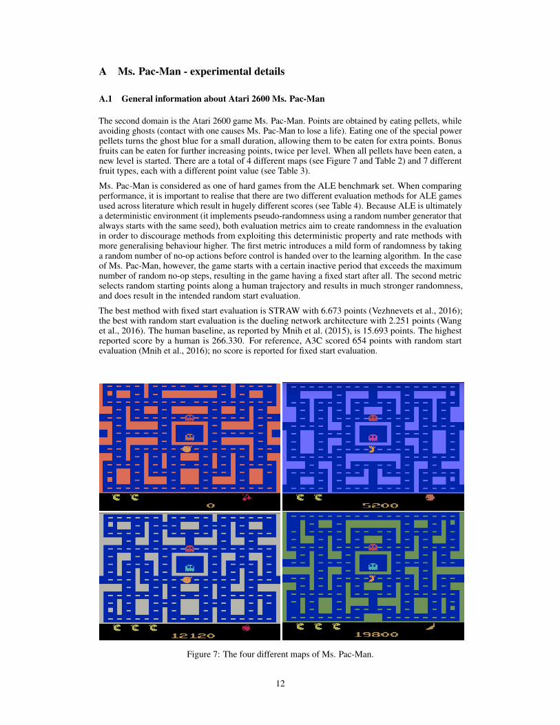
The second domain is the Atari 2600 game Ms. Pac-Man. Points are obtained by eating pellets, whileavoiding ghosts (contact with one causes Ms. Pac-Man to lose a life). Eating one of the special powerpellets turns the ghost blue for a small duration, allowing them to be eaten for extra points. Bonusfruits can be eaten for further increasing points, twice per level. When all pellets have been eaten, anew level is started. There are a total of 4 different maps (see Figure 7 and Table 2) and 7 differentfruit types, each with a different point value (see Table 3).

Ms. Pac-Man is considered as one of hard games from the ALE benchmark set. When comparingperformance, it is important to realise that there are two different evaluation methods for ALE gamesused across literature which result in hugely different scores (see Table 4). Because ALE is ultimatelya deterministic environment (it implements pseudo-randomness using a random number generator thatalways starts with the same seed), both evaluation metrics aim to create randomness in the evaluationin order to discourage methods from exploiting this deterministic property and rate methods withmore generalising behaviour higher. The first metric introduces a mild form of randomness by takinga random number of no-op actions before control is handed over to the learning algorithm. In the caseof Ms. Pac-Man, however, the game starts with a certain inactive period that exceeds the maximumnumber of random no-op steps, resulting in the game having a fixed start after all. The second metricselects random starting points along a human trajectory and results in much stronger randomness,and does result in the intended random start evaluation.

The best method with fixed start evaluation is STRAW with 6.673 points (Vezhnevets et al., 2016);the best with random start evaluation is the dueling network architecture with 2.251 points (Wanget al., 2016). The human baseline, as reported by Mnih et al. (2015), is 15.693 points. The highestreported score by a human is 266.330. For reference, A3C scored 654 points with random startevaluation (Mnih et al., 2016); no score is reported for fixed start evaluation.

Figure 7: The four different maps of Ms. Pac-Man.

12

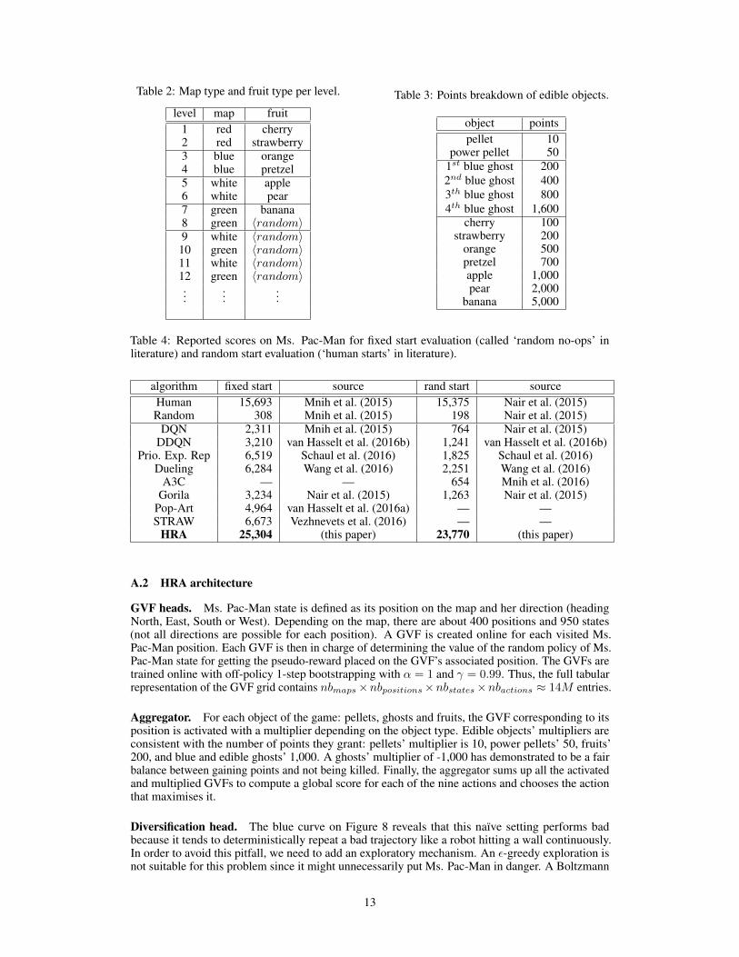
Table 2: Map type and fruit type per level.

level map fruit1 red cherry2 red strawberry3 blue orange4 blue pretzel5 white apple6 white pear7 green banana8 green 〈random〉9 white 〈random〉

10 green 〈random〉11 white 〈random〉12 green 〈random〉...

......

Table 3: Points breakdown of edible objects.

object pointspellet 10

power pellet 501st blue ghost 2002nd blue ghost 4003th blue ghost 8004th blue ghost 1,600

cherry 100strawberry 200

orange 500pretzel 700apple 1,000pear 2,000

banana 5,000

Table 4: Reported scores on Ms. Pac-Man for fixed start evaluation (called ‘random no-ops’ inliterature) and random start evaluation (‘human starts’ in literature).

algorithm fixed start source rand start sourceHuman 15,693 Mnih et al. (2015) 15,375 Nair et al. (2015)Random 308 Mnih et al. (2015) 198 Nair et al. (2015)

DQN 2,311 Mnih et al. (2015) 764 Nair et al. (2015)DDQN 3,210 van Hasselt et al. (2016b) 1,241 van Hasselt et al. (2016b)

Prio. Exp. Rep 6,519 Schaul et al. (2016) 1,825 Schaul et al. (2016)Dueling 6,284 Wang et al. (2016) 2,251 Wang et al. (2016)

A3C — — 654 Mnih et al. (2016)Gorila 3,234 Nair et al. (2015) 1,263 Nair et al. (2015)

Pop-Art 4,964 van Hasselt et al. (2016a) — —STRAW 6,673 Vezhnevets et al. (2016) — —

HRA 25,304 (this paper) 23,770 (this paper)

A.2 HRA architecture

GVF heads. Ms. Pac-Man state is defined as its position on the map and her direction (headingNorth, East, South or West). Depending on the map, there are about 400 positions and 950 states(not all directions are possible for each position). A GVF is created online for each visited Ms.Pac-Man position. Each GVF is then in charge of determining the value of the random policy of Ms.Pac-Man state for getting the pseudo-reward placed on the GVF’s associated position. The GVFs aretrained online with off-policy 1-step bootstrapping with α = 1 and γ = 0.99. Thus, the full tabularrepresentation of the GVF grid contains nbmaps×nbpositions×nbstates×nbactions ≈ 14M entries.

Aggregator. For each object of the game: pellets, ghosts and fruits, the GVF corresponding to itsposition is activated with a multiplier depending on the object type. Edible objects’ multipliers areconsistent with the number of points they grant: pellets’ multiplier is 10, power pellets’ 50, fruits’200, and blue and edible ghosts’ 1,000. A ghosts’ multiplier of -1,000 has demonstrated to be a fairbalance between gaining points and not being killed. Finally, the aggregator sums up all the activatedand multiplied GVFs to compute a global score for each of the nine actions and chooses the actionthat maximises it.

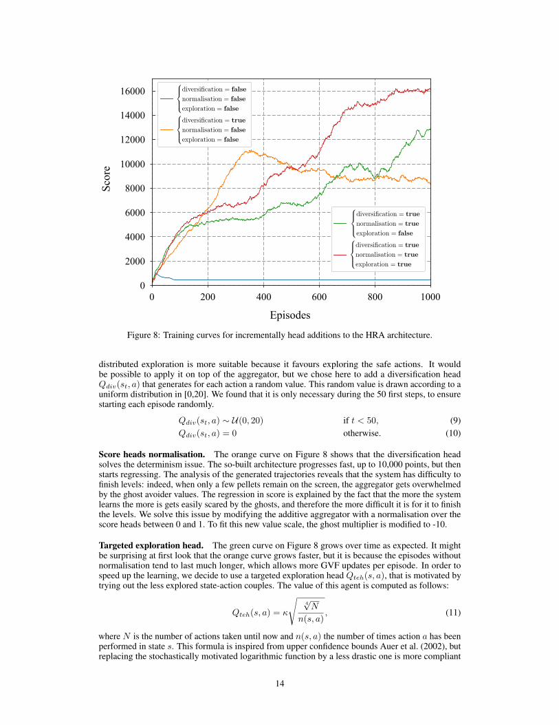
Diversification head. The blue curve on Figure 8 reveals that this naïve setting performs badbecause it tends to deterministically repeat a bad trajectory like a robot hitting a wall continuously.In order to avoid this pitfall, we need to add an exploratory mechanism. An ε-greedy exploration isnot suitable for this problem since it might unnecessarily put Ms. Pac-Man in danger. A Boltzmann

13

0

2000

4000

6000

8000

10000

12000

14000

16000

0 200 400 600 800 1000

Score

Episodes

Figure 8: Training curves for incrementally head additions to the HRA architecture.

distributed exploration is more suitable because it favours exploring the safe actions. It wouldbe possible to apply it on top of the aggregator, but we chose here to add a diversification headQdiv(st, a) that generates for each action a random value. This random value is drawn according to auniform distribution in [0,20]. We found that it is only necessary during the 50 first steps, to ensurestarting each episode randomly.

Qdiv(st, a) ∼ U(0, 20) if t < 50, (9)Qdiv(st, a) = 0 otherwise. (10)

Score heads normalisation. The orange curve on Figure 8 shows that the diversification headsolves the determinism issue. The so-built architecture progresses fast, up to 10,000 points, but thenstarts regressing. The analysis of the generated trajectories reveals that the system has difficulty tofinish levels: indeed, when only a few pellets remain on the screen, the aggregator gets overwhelmedby the ghost avoider values. The regression in score is explained by the fact that the more the systemlearns the more is gets easily scared by the ghosts, and therefore the more difficult it is for it to finishthe levels. We solve this issue by modifying the additive aggregator with a normalisation over thescore heads between 0 and 1. To fit this new value scale, the ghost multiplier is modified to -10.

Targeted exploration head. The green curve on Figure 8 grows over time as expected. It mightbe surprising at first look that the orange curve grows faster, but it is because the episodes withoutnormalisation tend to last much longer, which allows more GVF updates per episode. In order tospeed up the learning, we decide to use a targeted exploration head Qteh(s, a), that is motivated bytrying out the less explored state-action couples. The value of this agent is computed as follows:

Qteh(s, a) = κ

√4√N

n(s, a), (11)

where N is the number of actions taken until now and n(s, a) the number of times action a has beenperformed in state s. This formula is inspired from upper confidence bounds Auer et al. (2002), butreplacing the stochastically motivated logarithmic function by a less drastic one is more compliant

14

with our need for bootstrapping propagation. Note that this targeted exploration head is not areplacement for the diversification head. They are complementary: diversification for making eachtrajectory unique, and targeted exploration for prioritised exploration. The red curve on Figure 8reveals that the new targeted exploration head helps exploration and makes the learning faster. Thissetting constitutes the HRA architecture that is used in every experiment.

Executive memory head. When a human game player reaches the maximum of his cognitive andphysical ability, he starts to look for favourable situations or even glitches and memorises them. Thiscognitive process is referred as executive memory in cognitive science literature (Fuster, 2003; Glucket al., 2013). The executive memory head records every sequence of actions that led to pass a levelwithout any kill. Then, when facing the same level, the head gives a high value to the recorded action,in order to force the aggregator’s selection. Nota bene: since it does not allow generalisation, thishead is only employed for the level-passing experiment.

A.3 A3C baselines

Since we use low level features for the HRA architecture, we implement A3C and evaluate it both onthe pixel-based environment and on the low-level features. The implementation is performed in away to reproduce results of Mnih et al. (2015).

They are both trained similarly as in Mnih et al. (2016) on 8.108 frames, with γ = 0.99, entropyregularisation of 0.01, n-step return of 5, 16 threads, gradient clipping of 40, and α is set to take themaximum performance over the following values: [0.0001, 0.00025, 0.0005, 0.00075, 0.001]. Thepixel-based environment is a reproduction of the preprocessing and the network, except we only usea history of 2, because our steps are twice as long.

With the low features, five channels of a 40 by 40 map are used embedding the positions of Ms.Pac-Man, the pellets, the ghosts, the blue ghosts, and the special fruit. The input space is therefore5 by 40 by 40 plus the direction appended after convolutions: 2 of them with 16 (respectfully 32)filters of size 6 by 6 (respectfully 4 by 4) and subsampling of 2 by 2 and ReLU activation (for both).

0 1000 2000 3000 4000 50000

5000

10000

15000

20000

25000

HRA with = 0.95, = 0.95

HRA with = 0.95, = 0.97

HRA with = 0.95, = 0.99

HRA with = 0.97, = 0.95

HRA with = 0.97, = 0.97

HRA with = 0.97, = 0.99

HRA with = 0.99, = 0.95

HRA with = 0.99, = 0.97

HRA with = 0.99, = 0.99

Sco

re

Episodes

Figure 9: Gridsearch on γ values without executive memory smoothed over 500 episodes.

15

0 500 1000 1500 2000 2500 30000

20

40

60

80

100

120HRA with = 0.95, = 0.95

HRA with = 0.95, = 0.97

HRA with = 0.95, = 0.99

HRA with = 0.97, = 0.95

HRA with = 0.97, = 0.97

HRA with = 0.97, = 0.99

HRA with = 0.99, = 0.95

HRA with = 0.99, = 0.97

HRA with = 0.99, = 0.99

Lev

els

Pas

sed

Episodes

Figure 10: Gridsearch on γ values with executive memory.

Then, the network uses a hidden layer of 256 fully connected units with ReLU activation. Finally, thepolicy head has nbactions = 9 fully connected unit with softmax activation, and the value head has 1unit with a linear activation. All weights are uniformly initialised He et al. (2015).

A.4 Results

Training curves. Most of the results are already presented in the main document. For morecompleteness, we propose here the results of the gridsearch over γ values for both with and withoutthe executive memory. Values [0.95, 0.97, 0.99] have been tried independently for γscore and γghosts.

Figure 9 compares the training curves without executive memory. We can notice the following:

• all γ values turn out to yield very good results,• those good results generalise over random human starts (not shown),• high γ values for the ghosts tend to be better,• the γ value for the score is less impactful.

Figure 10 compares the training curves with executive memory. We can notice the following:

• the comments on Figure 9 are still holding,• it looks like that there is a bit more randomness in the level passing efficiency.

16