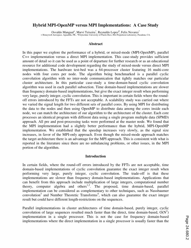
Paper ID #9953

Hybrid MPI-OpenMP versus MPI Implementations: A Case Study

Mr. Osvaldo Mangual, Honeywell Aerospace

Osvaldo Mangual has a Bachelor degree in Computer Engineering and a Master degree in ElectricalEngineering from Polytechnic University of Puerto Rico in the area of Digital Signal Processing. Hecurrently works at Honeywell Aerospace, PR, as a FPGA and ASIC Designer.

Dr. Marvi Teixeira, Polytechnic University of Puerto Rico

Dr. Teixeira is a Professor at the Electrical and Computer Engineering and Computer Science Departmentat Polytechnic University of Puerto Rico He holds a Ph.D. and MSEE degrees from University of PuertoRico at Mayaguez and a BSEE degree from Polytechnic University. Professor Teixeira is an IEEE SeniorMember, a Registered Professional Engineer and a former ASEE-Navy Summer Faculty Fellow.

Mr. Reynaldo Lopez-Roig, Polytechnic University of Puerto Rico

Mr. Lopez received his B.S. in Computer Engineering from the Polytechnic University of Puerto Rico in2013. His work as an undergraduate research assistant was related to the implementation and benchmark-ing of parallel signal processing algorithms in clusters and multicore architectures. Mr. Lopez is currentlyworking at the Jet Propulsion Laboratory as a Software Systems Engineer.

Prof. Felix Javier Nevarez-Ayala, Polytechnic University of Puerto Rico

Felix Nevarez is an Associate Professor in the Electrical and Computer Engineering Department at thePolytechnic University of Puerto Rico, He earned a BS in Physics and a MS in Electrical Engineeringfrom the University of Puerto Rico at Mayaguez and a BS in Electrical Engineering from the PolytechnicUniversity of Puerto Rico. HIs research interests are in numerical simulations and parallel and distributedprogramming.

c©American Society for Engineering Education, 2014

Page 24.680.1

Hybrid MPI-OpenMP versus MPI Implementations: A Case Study

Osvaldo Mangual+, Marvi Teixeira

*, Reynaldo Lopez

#, Felix Nevarez

*

+ Honeywell Aerospace, Aguadilla, PR., *Polytechnic University of Puerto Rico, #Jet Propulsion Laboratory, Pasadena, CA.

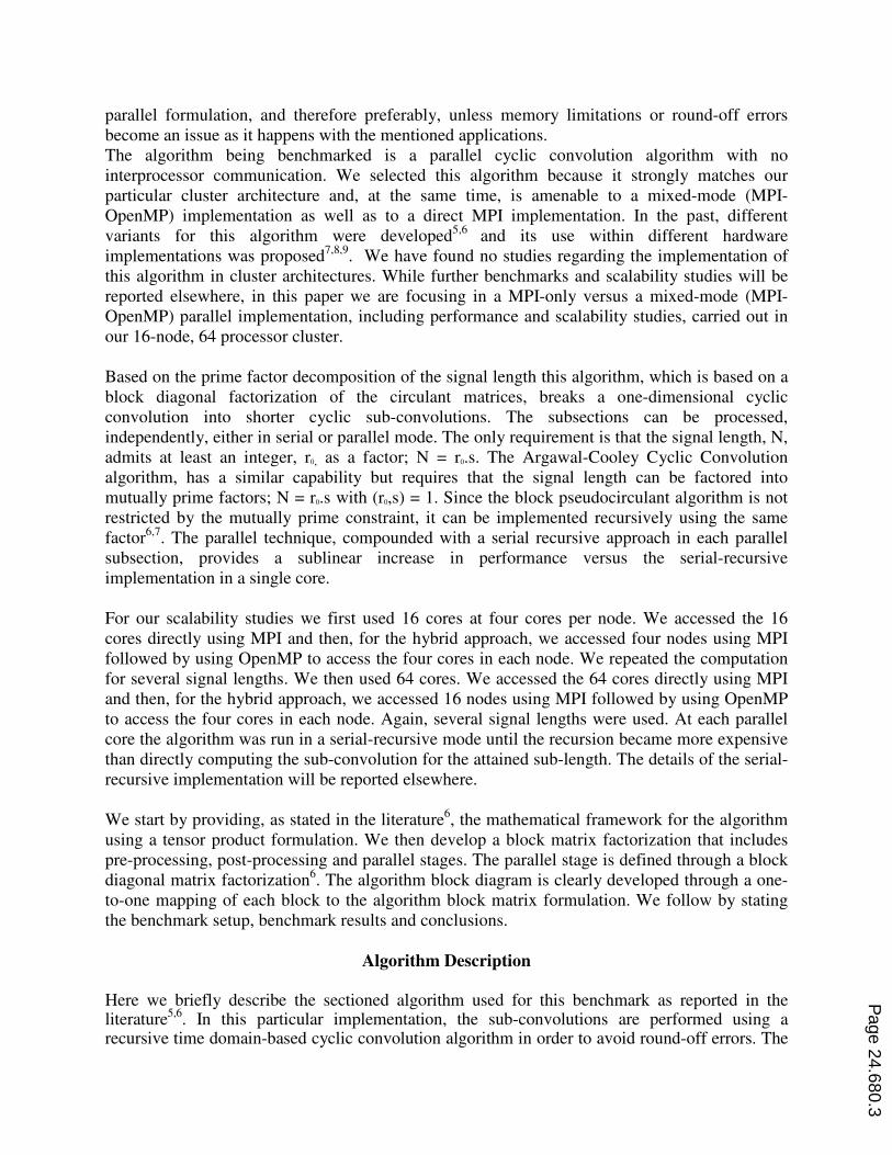
Abstract

In this paper we explore the performance of a hybrid, or mixed-mode (MPI-OpenMP), parallel

C++ implementation versus a direct MPI implementation. This case-study provides sufficient

amount of detail so it can be used as a point of departure for further research or as an educational

resource for additional code development regarding the study of mixed-mode versus direct MPI

implementations. The hardware test-bed was a 64-processor cluster featuring 16 multi-core

nodes with four cores per node. The algorithm being benchmarked is a parallel cyclic

convolution algorithm with no inter-node communication that tightly matches our particular

cluster architecture. In this particular case-study a time-domain-based cyclic convolution

algorithm was used in each parallel subsection. Time domain-based implementations are slower

than frequency domain-based implementations, but give the exact integer result when performing

very large, purely integer, cyclic convolution. This is important in certain fields where the round-

off errors introduced by the FFTs are not acceptable. A scalability study was carried out where

we varied the signal length for two different sets of parallel cores. By using MPI for distributing

the data to the nodes and then using OpenMP to distribute data among the cores inside each

node, we can match the architecture of our algorithm to the architecture of the cluster. Each core

processes an identical program with different data using a single program multiple data (SPMD)

approach. All pre and post-processing tasks were performed at the master node. We found that

the MPI implementation had a slightly better performance than the hybrid, MPI-OpenMP

implementation. We established that the speedup increases very slowly, as the signal size

increases, in favor of the MPI-only approach. Even though the mixed-mode approach matches

the target architecture there is an advantage for the MPI approach. This is consistent with what is

reported in the literature since there are no unbalancing problems, or other issues, in the MPI

portion of the algorithm.

Introduction

In certain fields, where the round-off errors introduced by the FFTs are not acceptable, time

domain-based implementations of cyclic convolution guarantee the exact integer result when

performing very large, purely integer, cyclic convolution. The trade-off is that these

implementations are slower than frequency domain-based implementations. Applications that

can benefit from this approach include multiplication of large integers, computational number

theory, computer algebra and others1,2

. The proposed, time domain-based, parallel

implementation can be considered as complementary to other techniques, such as Nussbaumer

convolution3 and Number Theoretic Transforms

4, which can also guarantee the exact integer

result but could have different length-restrictions on the sequences.

Parallel implementations in cluster architectures of time domain-based, purely integer, cyclic

convolution of large sequences resulted much faster than the direct, time domain-based, O(N2)

implementation in a single processor. This is not the case for frequency domain-based

implementations where the direct implementation in a single processor is usually faster than the

Page 24.680.2

parallel formulation, and therefore preferably, unless memory limitations or round-off errors

become an issue as it happens with the mentioned applications.

The algorithm being benchmarked is a parallel cyclic convolution algorithm with no

interprocessor communication. We selected this algorithm because it strongly matches our

particular cluster architecture and, at the same time, is amenable to a mixed-mode (MPI-

OpenMP) implementation as well as to a direct MPI implementation. In the past, different

variants for this algorithm were developed5,6

and its use within different hardware

implementations was proposed7,8,9

. We have found no studies regarding the implementation of

this algorithm in cluster architectures. While further benchmarks and scalability studies will be

reported elsewhere, in this paper we are focusing in a MPI-only versus a mixed-mode (MPI-

OpenMP) parallel implementation, including performance and scalability studies, carried out in

our 16-node, 64 processor cluster.

Based on the prime factor decomposition of the signal length this algorithm, which is based on a

block diagonal factorization of the circulant matrices, breaks a one-dimensional cyclic

convolution into shorter cyclic sub-convolutions. The subsections can be processed,

independently, either in serial or parallel mode. The only requirement is that the signal length, N,

admits at least an integer, r0, as a factor; N = r0.s. The Argawal-Cooley Cyclic Convolution

algorithm, has a similar capability but requires that the signal length can be factored into

mutually prime factors; N = r0.s with (r0,s) = 1. Since the block pseudocirculant algorithm is not

restricted by the mutually prime constraint, it can be implemented recursively using the same

factor6,7

. The parallel technique, compounded with a serial recursive approach in each parallel

subsection, provides a sublinear increase in performance versus the serial-recursive

implementation in a single core.

For our scalability studies we first used 16 cores at four cores per node. We accessed the 16

cores directly using MPI and then, for the hybrid approach, we accessed four nodes using MPI

followed by using OpenMP to access the four cores in each node. We repeated the computation

for several signal lengths. We then used 64 cores. We accessed the 64 cores directly using MPI

and then, for the hybrid approach, we accessed 16 nodes using MPI followed by using OpenMP

to access the four cores in each node. Again, several signal lengths were used. At each parallel

core the algorithm was run in a serial-recursive mode until the recursion became more expensive

than directly computing the sub-convolution for the attained sub-length. The details of the serial-

recursive implementation will be reported elsewhere.

We start by providing, as stated in the literature6, the mathematical framework for the algorithm

using a tensor product formulation. We then develop a block matrix factorization that includes

pre-processing, post-processing and parallel stages. The parallel stage is defined through a block

diagonal matrix factorization6. The algorithm block diagram is clearly developed through a one-

to-one mapping of each block to the algorithm block matrix formulation. We follow by stating

the benchmark setup, benchmark results and conclusions.

Algorithm Description

Here we briefly describe the sectioned algorithm used for this benchmark as reported in the literature

5,6. In this particular implementation, the sub-convolutions are performed using a

recursive time domain-based cyclic convolution algorithm in order to avoid round-off errors. The

Page 24.680.3

proposed algorithmic implementation does not require communication among cores but involves initial and final data distribution at the pre-processing and post-processing stages. Cyclic convolution is a established technique broadly used in signal processing applications.

The Discrete Cosine Transform and the Discrete Fourier Transform, for example, can be

formulated and implemented as cyclic convolutions6,7

. In particular, parallel processing of cyclic

convolution has potential advantages in terms of speed and/or access to extended memory, but

requires breaking the original cyclic convolution into independent sub-convolution sections. The

Agarwal-Cooley cyclic convolution algorithm is suitable to this task but requires that the

convolution length be factored into mutually prime factors, thus imposing a tight constraint on its

application3. There are also multidimensional methods but they may require the lengths along

some dimensions to be doubled3. There other recursive methods, which are also constrained in

terms of signal length3. When the mentioned constraints are not practical, this algorithm provides

a complementary alternative since it only requires that the convolution length be factorable5,6

.

This technique, depending on the prime factor decomposition of the signal length, can be

combined with the Agarwal-Cooley algorithm or with other techniques.

By conjugating the circulant matrix with stride permutations a block pseudocirculant formulation

is obtained. Each circular sub-block can be independently processed as a cyclic sub-convolution.

Recursion can be applied, in either a parallel, serial or combined fashion, by using the same

technique in each cyclic sub-convolution. The final sub-convolutions at the bottom of the

recursion can be performed using any method. The basic formulation of the algorithm as stated

in the literature is as follows6,

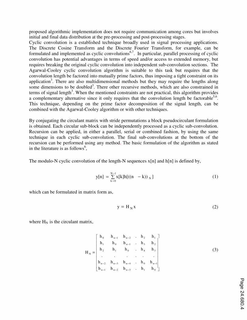
The modulo-N cyclic convolution of the length-N sequences x[n] and h[n] is defined by,

∑ −=−

=

1N

0kN ]k))x[k]h[((ny[n] (1)

which can be formulated in matrix form as,

xHy N= (2)

where HN is the circulant matrix,

−−−

−−−−

−

−−

=

013n2n1n

1n04n3n2n

34012

231n01

122n1n0

N

hh.hhh

hh.hhh

......

hh.hhh

hh.hhh

hh.hhh

H (3)

Page 24.680.4

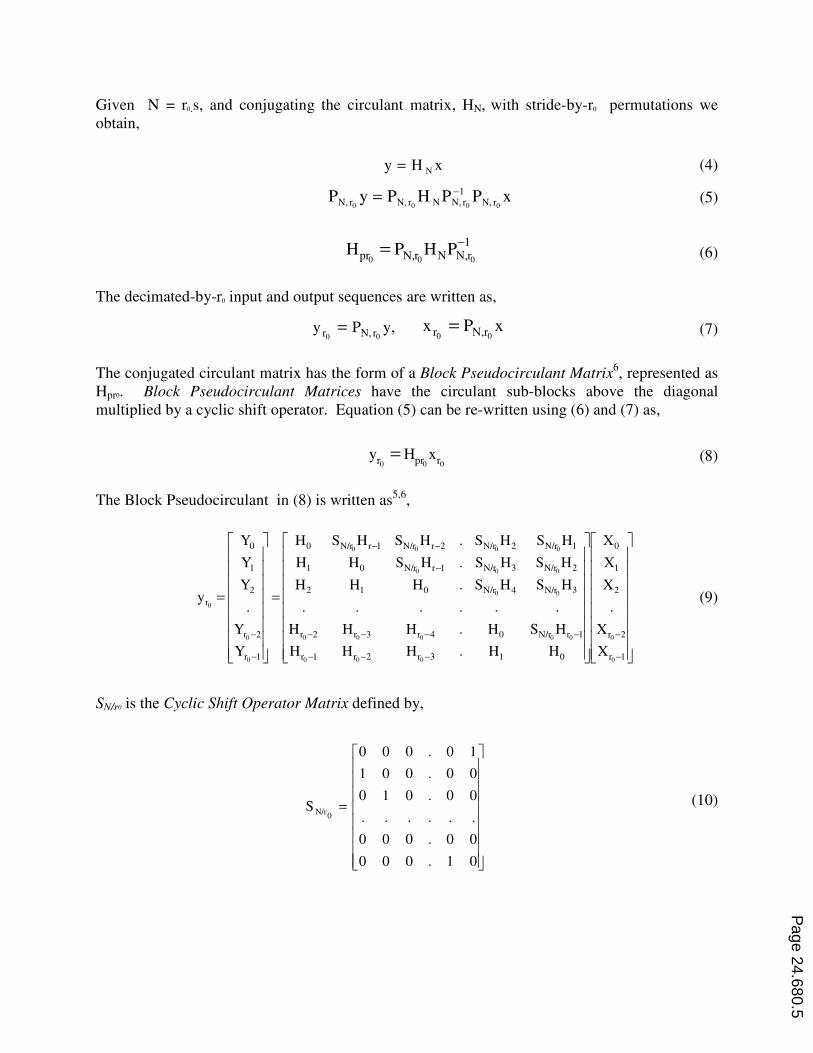
Given N = r0.s, and conjugating the circulant matrix, HN, with stride-by-r0 permutations we

obtain,

xHy N= (4)

xPPHPyP0000 rN,

1rN,NrN,rN,

−= (5)

1rN,NrN,pr 000

PHPH−

= (6)

The decimated-by-r0 input and output sequences are written as,

,yPy00 rN,r = xPx

00 rN,r = (7)

The conjugated circulant matrix has the form of a Block Pseudocirculant Matrix6, represented as

Hpr0. Block Pseudocirculant Matrices have the circulant sub-blocks above the diagonal

multiplied by a cyclic shift operator. Equation (5) can be re-written using (6) and (7) as,

000 rprr xHy = (8)

The Block Pseudocirculant in (8) is written as5,6

,

=

=

−

−

−−−

−−−−

−

−−

−

−

1r

2r

2

1

0

013r2r1r

1rN/r04r3r2r

3N/r4N/r012

2N/r3N/r1rN/r01

1N/r2N/r2rN/r1rN/r0

1r

2r

2

1

0

r

0

0

000

00000

00

000

0000

0

0

0

X

X

.

X

X

X

HH.HHH

HSH.HHH

......

HSHS.HHH

HSHS.HSHH

HSHS.HSHSH

Y

Y

.

Y

Y

Y

y

(9)

SN/r0 is the Cyclic Shift Operator Matrix defined by,

=

01.000

00.000

......

00.010

00.001

10.000

S0

N/r (10)

Page 24.680.5

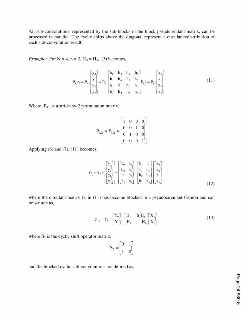
All sub-convolutions, represented by the sub-blocks in the block pseudcirculant matrix, can be

processed in parallel. The cyclic shifts above the diagonal represent a circular redistribution of

each sub-convolution result.

Example: For N = 4, r0 = 2, HN = H4, (5) becomes,

===−

3

2

1

0

4,21

4,2

0123

3012

2301

1230

4,2

3

2

1

0

4,24,2

x

x

x

x

PP

hhhh

hhhh

hhhh

hhhh

P

y

y

y

y

PyP

(11)

Where P4,2 is a stride-by-2 permutation matrix,

==

1000

0010

0100

0001

PP1-

4,24,2

Applying (6) and (7), (11) becomes,

===

3

1

2

0

02

20

13

31

31

13

02

20

3

1

2

0

20

x

x

x

x

hh

hh

hh

hh

hh

hh

hh

hh

y

y

y

y

yry

(12)

where the circulant matrix H4 in (11) has become blocked in a pseudocirculant fashion and can

be written as,

===

1

0

01

120

1

0

20 X

X

H H

HSH

Y

Yyry (13)

where S2 is the cyclic shift operator matrix,

=

01

102S

and the blocked cyclic sub-convolutions are defined as,

Page 24.680.6

=

02

20

0hh

hhH ,

=

13

31

1hh

hhH (14)

Further examples can be found in the literature6,7

. It is clear that each sub-convolution can be

separately processed, followed by a reconstruction stage to provide the final result. Parallel

algorithms can be developed by factorization of the Block Pseudocirculant matrix shown in (9),

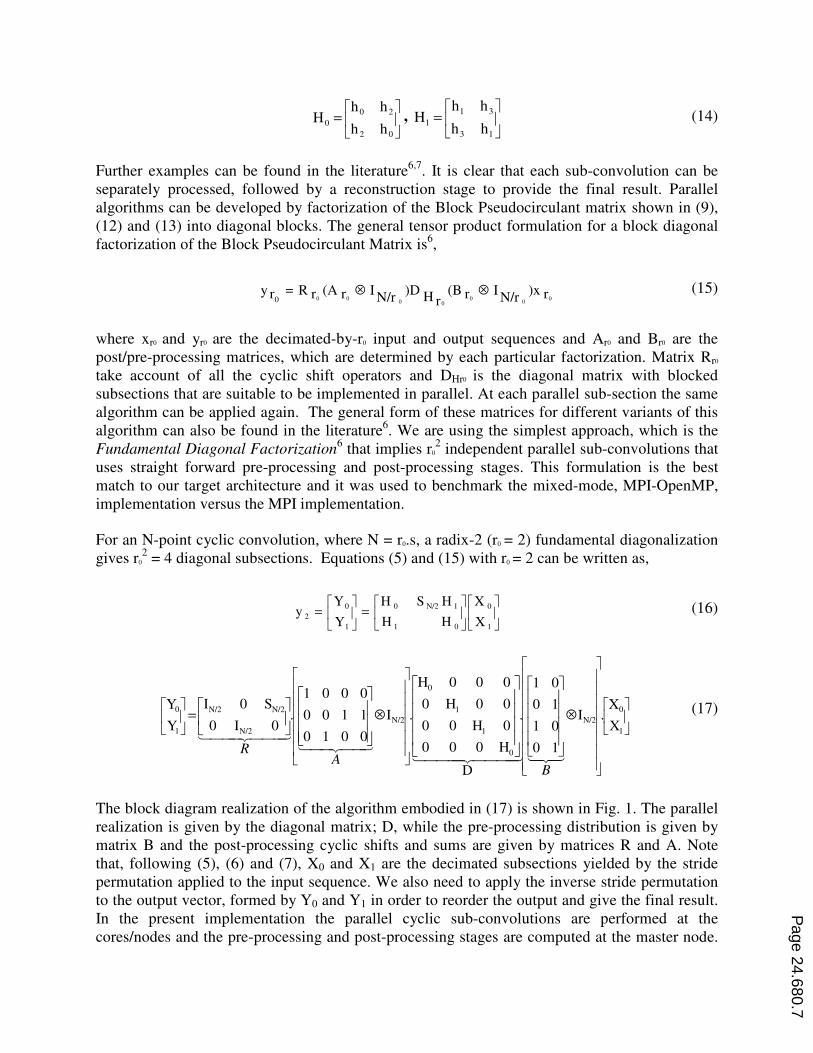
(12) and (13) into diagonal blocks. The general tensor product formulation for a block diagonal

factorization of the Block Pseudocirculant Matrix is6,

00

000

00 r)xN/r

Ir(BrH

)DN/r

Ir(ArRry0

⊗⊗= (15)

where xr0 and yr0 are the decimated-by-r0 input and output sequences and Ar0 and Br0 are the

post/pre-processing matrices, which are determined by each particular factorization. Matrix Rr0

take account of all the cyclic shift operators and DHr0 is the diagonal matrix with blocked

subsections that are suitable to be implemented in parallel. At each parallel sub-section the same

algorithm can be applied again. The general form of these matrices for different variants of this

algorithm can also be found in the literature6. We are using the simplest approach, which is the

Fundamental Diagonal Factorization6 that implies r0

2 independent parallel sub-convolutions that

uses straight forward pre-processing and post-processing stages. This formulation is the best

match to our target architecture and it was used to benchmark the mixed-mode, MPI-OpenMP,

implementation versus the MPI implementation.

For an N-point cyclic convolution, where N = r0.s, a radix-2 (r0 = 2) fundamental diagonalization

gives r0

2 = 4 diagonal subsections. Equations (5) and (15) with r0 = 2

can be written as,

==

1

0

01

1N/20

1

0

2X

X

H H

HSH

Y

Yy (16)

⊗

⊗

=

1

0

N/2

0

1

1

0

N/2

N/2

N/2N/2

1

0

X

X.I

10

01

10

01

D

.

H000

0H00

00H0

000H

.I

0010

1100

0001

.0I0

S0I

Y

Y

434214444 34444 2144 344 21

444 3444 21

BA

R

(17)

The block diagram realization of the algorithm embodied in (17) is shown in Fig. 1. The parallel

realization is given by the diagonal matrix; D, while the pre-processing distribution is given by

matrix B and the post-processing cyclic shifts and sums are given by matrices R and A. Note

that, following (5), (6) and (7), X0 and X1 are the decimated subsections yielded by the stride

permutation applied to the input sequence. We also need to apply the inverse stride permutation

to the output vector, formed by Y0 and Y1 in order to reorder the output and give the final result.

In the present implementation the parallel cyclic sub-convolutions are performed at the

cores/nodes and the pre-processing and post-processing stages are computed at the master node.

Page 24.680.7

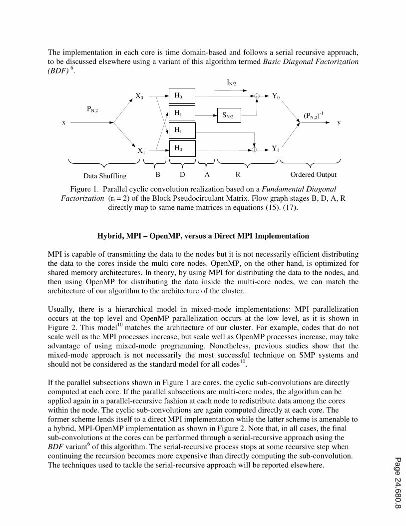
The implementation in each core is time domain-based and follows a serial recursive approach,

to be discussed elsewhere using a variant of this algorithm termed Basic Diagonal Factorization

(BDF) 6.

Figure 1. Parallel cyclic convolution realization based on a Fundamental Diagonal

Factorization (r0 = 2) of the Block Pseudocirculant Matrix. Flow graph stages B, D, A, R

directly map to same name matrices in equations (15). (17).

Hybrid, MPI – OpenMP, versus a Direct MPI Implementation

MPI is capable of transmitting the data to the nodes but it is not necessarily efficient distributing

the data to the cores inside the multi-core nodes. OpenMP, on the other hand, is optimized for

shared memory architectures. In theory, by using MPI for distributing the data to the nodes, and

then using OpenMP for distributing the data inside the multi-core nodes, we can match the

architecture of our algorithm to the architecture of the cluster.

Usually, there is a hierarchical model in mixed-mode implementations: MPI parallelization

occurs at the top level and OpenMP parallelization occurs at the low level, as it is shown in

Figure 2. This model10

matches the architecture of our cluster. For example, codes that do not

scale well as the MPI processes increase, but scale well as OpenMP processes increase, may take

advantage of using mixed-mode programming. Nonetheless, previous studies show that the

mixed-mode approach is not necessarily the most successful technique on SMP systems and

should not be considered as the standard model for all codes10

.

If the parallel subsections shown in Figure 1 are cores, the cyclic sub-convolutions are directly

computed at each core. If the parallel subsections are multi-core nodes, the algorithm can be

applied again in a parallel-recursive fashion at each node to redistribute data among the cores

within the node. The cyclic sub-convolutions are again computed directly at each core. The

former scheme lends itself to a direct MPI implementation while the latter scheme is amenable to

a hybrid, MPI-OpenMP implementation as shown in Figure 2. Note that, in all cases, the final

sub-convolutions at the cores can be performed through a serial-recursive approach using the

BDF variant6 of this algorithm. The serial-recursive process stops at some recursive step when

continuing the recursion becomes more expensive than directly computing the sub-convolution.

The techniques used to tackle the serial-recursive approach will be reported elsewhere.

H0

H1

H1

H0

SN/2

X1

Y1

X0

x

IN/2

PN,2

Y0

y

(PN,2)-1

B D A R Ordered Output Data Shuffling

Page 24.680.8

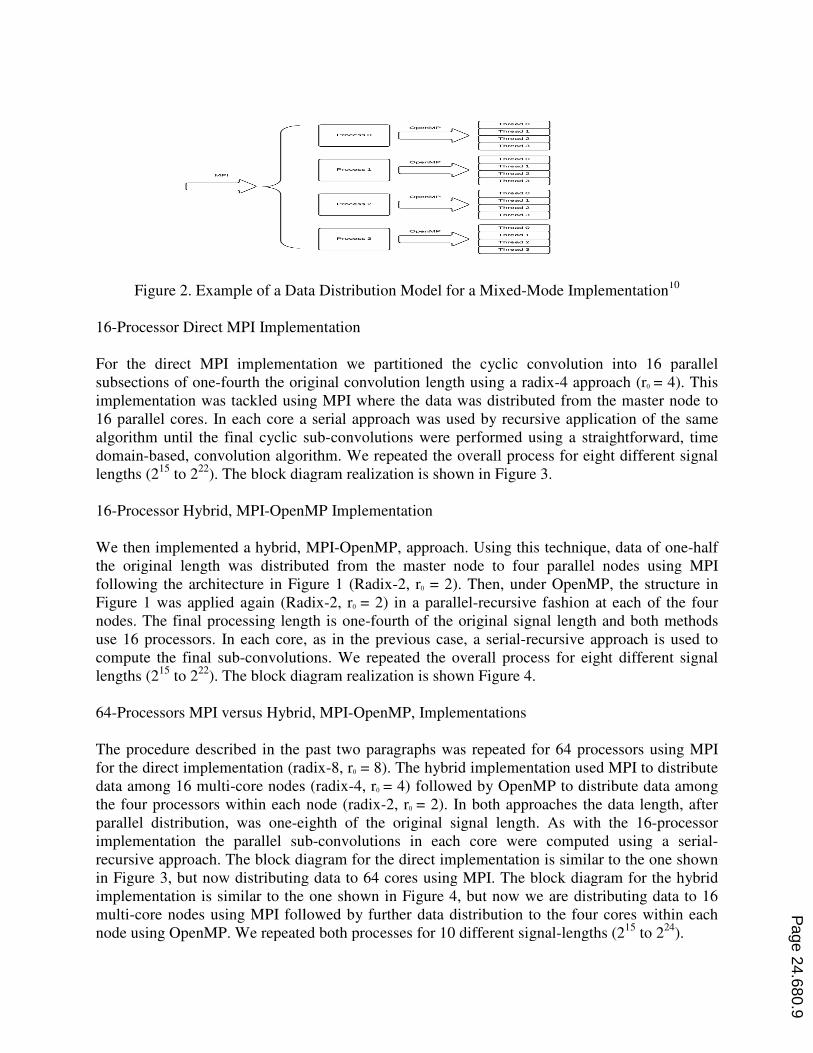
Figure 2. Example of a Data Distribution Model for

16-Processor Direct MPI Implementation

For the direct MPI implementation we

subsections of one-fourth the original convolution length using a radix

implementation was tackled using MPI where the data was distributed from the master node to

16 parallel cores. In each core a serial approach was used by

algorithm until the final cyclic sub

domain-based, convolution algorithm.

lengths (215

to 222

). The block diagram realization is show

16-Processor Hybrid, MPI-OpenMP Implementation

We then implemented a hybrid,

the original length was distributed from the master node to four

following the architecture in Figure 1

Figure 1 was applied again (Radix

nodes. The final processing length is one

use 16 processors. In each core, as in the previous case, a serial

compute the final sub-convolutions. We repeated the

lengths (215

to 222

). The block diagram re

64-Processors MPI versus Hybrid

The procedure described in the past two paragraphs was repeated for

for the direct implementation (radix

data among 16 multi-core nodes (radix

the four processors within each node (radix

parallel distribution, was one-eighth of the original signal length. As

implementation the parallel sub

recursive approach. The block diagram for the direct implementation is similar to th

in Figure 3, but now distributing

implementation is similar to the one shown in Figure 4, but now we are distributing

multi-core nodes using MPI followed by

node using OpenMP. We repeated both processes for 10 different signal

. Example of a Data Distribution Model for a Mixed-Mode Implementation

Processor Direct MPI Implementation

For the direct MPI implementation we partitioned the cyclic convolution into 16 parallel

the original convolution length using a radix-4 approach

implementation was tackled using MPI where the data was distributed from the master node to

In each core a serial approach was used by recursive application of th

sub-convolutions were performed using a straightforward,

convolution algorithm. We repeated the overall process for eight different signal

The block diagram realization is shown in Figure 3.

OpenMP Implementation

hybrid, MPI-OpenMP, approach. Using this technique,

the original length was distributed from the master node to four parallel nodes using MPI

the architecture in Figure 1 (Radix-2, r0 = 2). Then, under OpenMP

(Radix-2, r0 = 2) in a parallel-recursive fashion at each of the four

nodes. The final processing length is one-fourth of the original signal length and both method

re, as in the previous case, a serial-recursive approach is used to

convolutions. We repeated the overall process for eight different signal

. The block diagram realization is shown Figure 4.

Hybrid, MPI-OpenMP, Implementations

The procedure described in the past two paragraphs was repeated for 64 processors using MPI

for the direct implementation (radix-8, r0 = 8). The hybrid implementation used MPI to distribute

core nodes (radix-4, r0 = 4) followed by OpenMP to distribute data among

the four processors within each node (radix-2, r0 = 2). In both approaches the data length, after

eighth of the original signal length. As with

parallel sub-convolutions in each core were computed using a serial

The block diagram for the direct implementation is similar to th

distributing data to 64 cores using MPI. The block diagram for the hybrid

implementation is similar to the one shown in Figure 4, but now we are distributing

core nodes using MPI followed by further data distribution to the four cores within each

We repeated both processes for 10 different signal-lengths (2

Implementation

10

partitioned the cyclic convolution into 16 parallel

4 approach (r0 = 4). This

implementation was tackled using MPI where the data was distributed from the master node to

application of the same

straightforward, time

process for eight different signal

, data of one-half

nodes using MPI

under OpenMP, the structure in

at each of the four

ngth and both methods

recursive approach is used to

process for eight different signal

64 processors using MPI

= 8). The hybrid implementation used MPI to distribute

= 4) followed by OpenMP to distribute data among

= 2). In both approaches the data length, after

the 16-processor

convolutions in each core were computed using a serial-

The block diagram for the direct implementation is similar to the one shown

64 cores using MPI. The block diagram for the hybrid

implementation is similar to the one shown in Figure 4, but now we are distributing data to 16

cores within each

lengths (215

to 224

).

Page 24.680.9

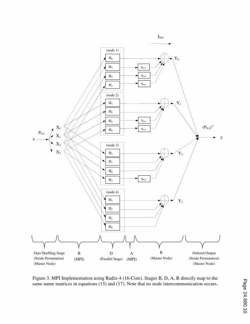
Figure 3. MPI Implementation using Radix-4 (16-Core). Stages B, D, A, R directly map to the

same name matrices in equations (15) and (17). Note that no node intercommunication occurs.

X1

X0

x

IN/4

PN,4

Y0

y

(PN,4)-1

B

(MPI)

D

(Parallel Stage)

A

(MPI)

R

(Master Node)

H0

H3

H2

H1

SN/4

(node 1)

Data Shuffling Stage

(Stride Permutation)

(Master Node)

Ordered Output

(Stride Permutation)

(Master Node)

X2

X3

SN/4

SN/4

Y1 H1

H3

H2

(node 2)

SN/4

SN/4

H0

Y2 H2

H0

H3

(node 3)

SN/4

H1

Y3 H3

H1

H0

(node 4)

H2

Page 24.680.10

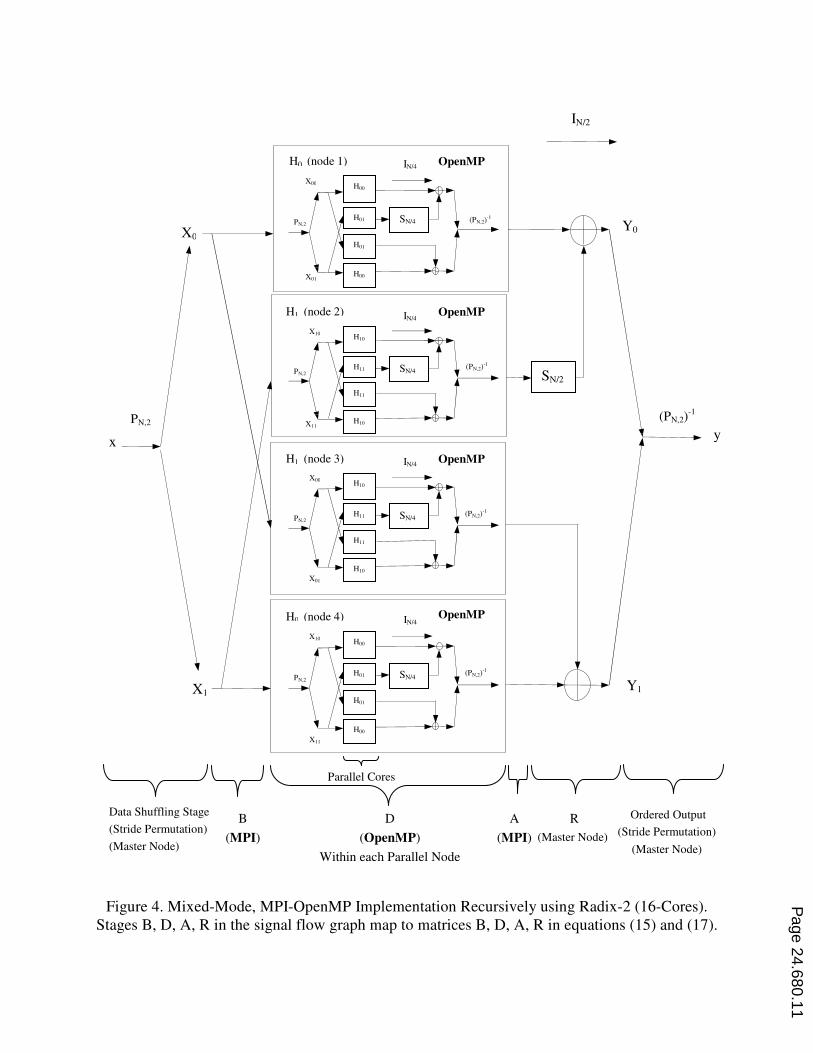
Figure 4. Mixed-Mode, MPI-OpenMP Implementation Recursively using Radix-2 (16-Cores).

Stages B, D, A, R in the signal flow graph map to matrices B, D, A, R in equations (15) and (17).

SN/2

X1 Y1

X0

x

IN/2

PN,2

Y0

y

(PN,2)-1

B

(MPI)

D

(OpenMP)

Within each Parallel Node

A

(MPI)

R

(Master Node)

H00

H01

H01

H00

SN/4

IN/4

PN,2

H10

H11

H11

H10

SN/4

IN/4

PN,2

H10

H11

H11

H10

SN/4

IN/4

PN,2

H0 (node 1)

H1 (node 2)

H1 (node 3)

H0 (node 4)

OpenMP

OpenMP

OpenMP

OpenMP

Data Shuffling Stage

(Stride Permutation)

(Master Node)

Ordered Output

(Stride Permutation)

(Master Node)

(PN,2)-1

(PN,2)-1

(PN,2)-1

H00

H01

H01

H00

SN/4

IN/4

PN,2

(PN,2)-1

Parallel Cores

X00

X01

X11

X01

X10

X00

X10

X11

Page 24.680.11

Hardware Setup

Hardware Setup: 16-Nodes, 64 Processors, Dell Cluster

The current benchmark was carried out using a 16-node cluster with multi-core nodes. Each node

has two, dual-core processors for a total of 64 cores. The cluster is somewhat dated but still

useful for comparative and scalability studies. The cluster hardware specifications are:

Master Node:

• Brand: Dell PowerEdge 1950

• Processor: 2 X Intel Xenon Dempsey 5050, 80555K @ 3.0 GHz (Dual-Core

Processor). 667MHz FSB. L1 Cache Data: 2 x 16KB, L2 Cache: 2 x 2MB.

• Main Memory: 2GB DDR2-533, 533MHz.

• Secondary Memory: 2 X 36GB @ 15K RPM.

• Operating System: CentOS Linux 5.6 64-bit.

Compute Nodes:

• Brand: Dell PowerEdge SC1435

• Processor: 2 X AMD 2210 @ 1.8GHz (Dual-Core Processor). L1 Cache Data: 2 x

128KB, L2 Cache: 2 x 1MB.

• Main Memory: 4GB DDR2-667, 667MHz.

• Secondary Memory: 80GB @ 7.2K RPM.

• Operating System: Linux 64-bit.

Software: C++

Benchmark Results

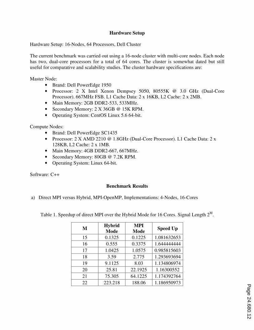
a) Direct MPI versus Hybrid, MPI-OpenMP, Implementations: 4-Nodes, 16-Cores

Table 1. Speedup of direct MPI over the Hybrid Mode for 16 Cores. Signal Length 2M

.

M Hybrid

Mode

MPI

Mode Speed Up

15 0.1325 0.1225 1.081632653

16 0.555 0.3375 1.644444444

17 1.0425 1.0575 0.985815603

18 3.59 2.775 1.293693694

19 9.1125 8.03 1.134806974

20 25.81 22.1925 1.16300552

21 75.305 64.1225 1.174392764

22 223.218 188.06 1.186950973

Page 24.680.12

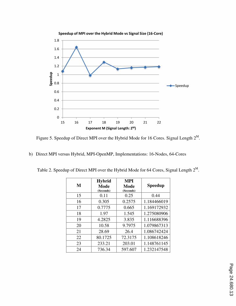
Figure 5. Speedup of Direct

b) Direct MPI versus Hybrid, MPI

Table 2. Speedup of Direct

M

15

16

17

18

19

20

21

22

23

24

0

0.2

0.4

0.6

0.8

1

1.2

1.4

1.6

1.8

15 16 17

Sp

ee

du

p

Exponent M (Signal Length: 2

Speedup of MPI over the Hybrid Mode vs Signal Size (16

Direct MPI over the Hybrid Mode for 16 Cores. Signal Length 2

Direct MPI versus Hybrid, MPI-OpenMP, Implementations: 16-Nodes, 64-Cores

Direct MPI over the Hybrid Mode for 64 Cores, Signal Length 2

Hybrid

Mode (Seconds)

MPI

Mode (Seconds)

Speedup

0.11 0.25 0.44

0.305 0.2575 1.184466019

0.7775 0.665 1.169172932

1.97 1.545 1.275080906

4.2825 3.835 1.116688396

10.58 9.7975 1.079867313

28.69 26.4 1.086742424

80.1725 72.3175 1.108618246

233.21 203.01 1.148761145

736.34 597.607 1.232147548

17 18 19 20 21 22

Exponent M (Signal Length: 2M)

Speedup of MPI over the Hybrid Mode vs Signal Size (16-Core)

Speedup

Signal Length 2

M.

Cores

Signal Length 2M

.

Speedup

Page 24.680.13

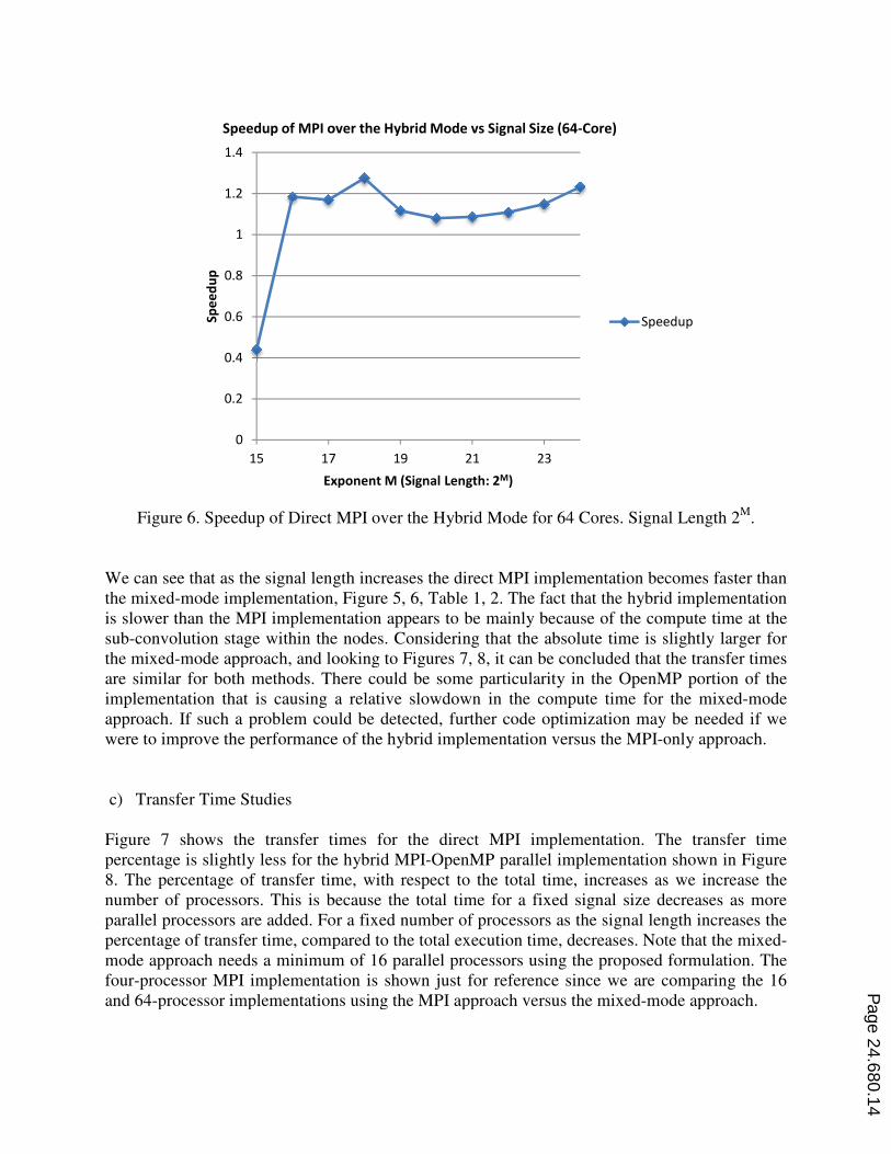
Figure 6. Speedup of Direct

We can see that as the signal length increases the direct MPI implementation becomes faster than

the mixed-mode implementation

is slower than the MPI implementation appears to be mainly because of

sub-convolution stage within the nodes

the mixed-mode approach, and looking to Figures 7, 8, it can be concluded that

are similar for both methods. There

implementation that is causing a

approach. If such a problem could

were to improve the performance of the

c) Transfer Time Studies

Figure 7 shows the transfer times for the

percentage is slightly less for the

8. The percentage of transfer time

number of processors. This is because the total time

parallel processors are added. For a fixed number of processors

percentage of transfer time, compared to the total execution time

mode approach needs a minimum of 16 parallel

four-processor MPI implementation is shown just for reference since we are

and 64-processor implementations using the MPI approach versus the mixed

0

0.2

0.4

0.6

0.8

1

1.2

1.4

15 17

Sp

ee

du

p

Exponent M (Signal Length: 2

Speedup of MPI over the Hybrid Mode vs Signal Size (64

Direct MPI over the Hybrid Mode for 64 Cores. Signal Length 2

We can see that as the signal length increases the direct MPI implementation becomes faster than

implementation, Figure 5, 6, Table 1, 2. The fact that the hybrid

mplementation appears to be mainly because of the compute time at the

the nodes. Considering that the absolute time is slightly larger for

mode approach, and looking to Figures 7, 8, it can be concluded that the trans

. There could be some particularity in the OpenMP portion of the

that is causing a relative slowdown in the compute time for the mixed

ould be detected, further code optimization may be needed if we

performance of the hybrid implementation versus the MPI-only approach

shows the transfer times for the direct MPI implementation. The transfer time

the hybrid MPI-OpenMP parallel implementation

percentage of transfer time, with respect to the total time, increases as we increase the

number of processors. This is because the total time for a fixed signal size decreas

For a fixed number of processors as the signal length

compared to the total execution time, decreases. Note that

mode approach needs a minimum of 16 parallel processors using the proposed formulation.

implementation is shown just for reference since we are comparing the 16

processor implementations using the MPI approach versus the mixed-mode approach.

17 19 21 23

Exponent M (Signal Length: 2M)

Speedup of MPI over the Hybrid Mode vs Signal Size (64-Core)

Speedup

Signal Length 2

M.

We can see that as the signal length increases the direct MPI implementation becomes faster than

hybrid implementation

compute time at the

Considering that the absolute time is slightly larger for

the transfer times

in the OpenMP portion of the

for the mixed-mode

imization may be needed if we

only approach.

The transfer time

parallel implementation shown in Figure

increases as we increase the

decreases as more

as the signal length increases the

Note that the mixed-

processors using the proposed formulation. The

comparing the 16

mode approach.

Speedup

Page 24.680.14

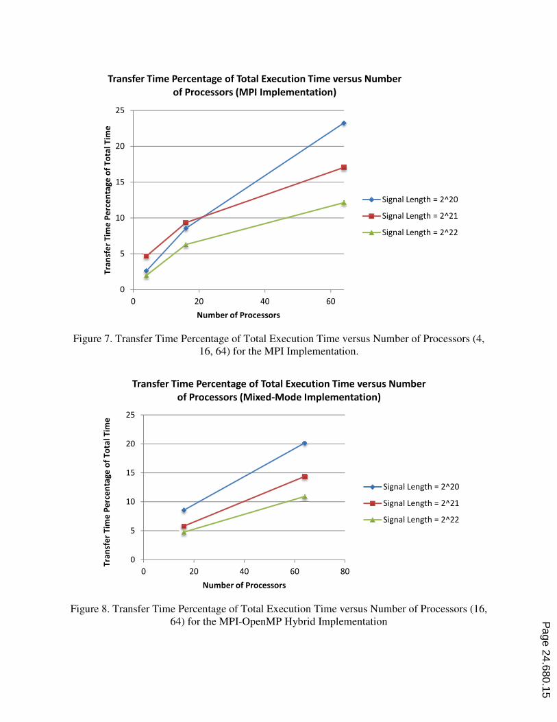
Figure 7. Transfer Time Percent

16, 64)

Figure 8. Transfer Time Percent

64) for the

0

5

10

15

20

25

0 20

Tra

nsf

er

Tim

e P

erc

en

tag

e o

f T

ota

l T

ime

Number of Processors

Transfer Time Percentage of Total Execution Time versus Number

of Processors (MPI Implementation)

0

5

10

15

20

25

0 20

Tra

nsf

er

Tim

e P

erc

en

tag

e o

f T

ota

l T

ime

Number of Processors

Transfer Time Percentage of Total Execution Time versus Number

of Processors (Mixed

centage of Total Execution Time versus Number of Processors

16, 64) for the MPI Implementation.

. Transfer Time Percentage of Total Execution Time versus Number of Processors

for the MPI-OpenMP Hybrid Implementation

40 60

Number of Processors

Transfer Time Percentage of Total Execution Time versus Number

of Processors (MPI Implementation)

Signal Length = 2^20

Signal Length = 2^21

Signal Length = 2^22

40 60 80

Number of Processors

Transfer Time Percentage of Total Execution Time versus Number

of Processors (Mixed-Mode Implementation)

Signal Length = 2^20

Signal Length = 2^21

Signal Length = 2^22

of Total Execution Time versus Number of Processors (4,

of Total Execution Time versus Number of Processors (16,

Signal Length = 2^20

Signal Length = 2^21

Signal Length = 2^22

Transfer Time Percentage of Total Execution Time versus Number

Signal Length = 2^20

Signal Length = 2^21

Signal Length = 2^22

Page 24.680.15

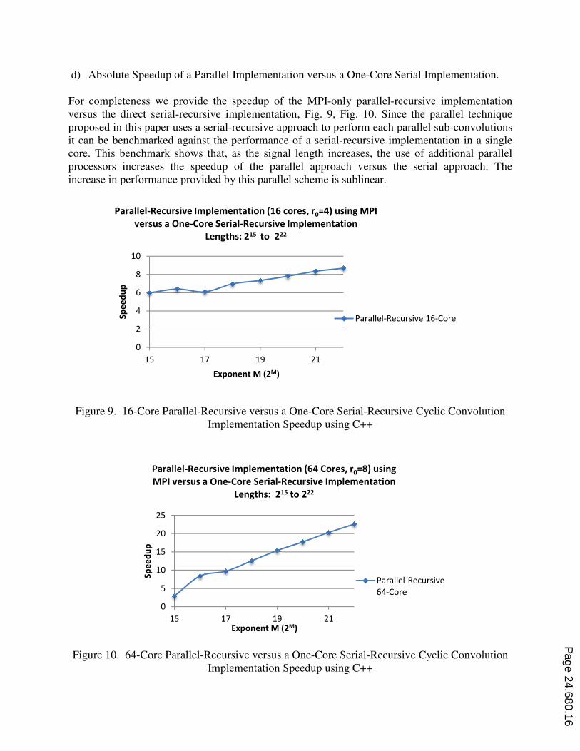
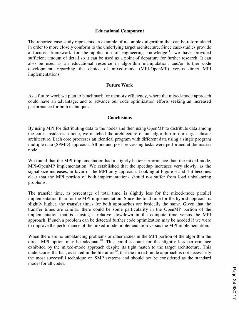
d) Absolute Speedup of a Parallel Implementation

For completeness we provide the

versus the direct serial-recursive implementation

proposed in this paper uses a serial

it can be benchmarked against the performance of a serial

core. This benchmark shows that, as the sign

processors increases the speedup

increase in performance provided by this parallel scheme

Figure 9. 16-Core Parallel-Recursive

Implementation

Figure 10. 64-Core Parallel-Recursive v

Implementation Speedup using C++

0

2

4

6

8

10

15 17

Sp

ee

du

p

Exponent M (2

Parallel-Recursive Implementation (16 cores, r

versus a One-Core Serial

Lengths: 2

0

5

10

15

20

25

15

Sp

ee

du

p

Parallel-Recursive Implementation (64 Cores,

MPI versus a One

llel Implementation versus a One-Core Serial Implementation.

For completeness we provide the speedup of the MPI-only parallel-recursive implementation

recursive implementation, Fig. 9, Fig. 10. Since the parallel technique

uses a serial-recursive approach to perform each parallel

the performance of a serial-recursive implementation

This benchmark shows that, as the signal length increases, the use of additional

speedup of the parallel approach versus the serial approach.

provided by this parallel scheme is sublinear.

Recursive versus a One-Core Serial-Recursive Cyclic Convolution

Implementation Speedup using C++

Recursive versus a One-Core Serial-Recursive Cyclic Convolution

Implementation Speedup using C++

19 21

Exponent M (2M)

Recursive Implementation (16 cores, r0=4) using MPI

Core Serial-Recursive Implementation

Lengths: 215 to 222

Parallel-Recursive 16

17 19 21Exponent M (2M)

Recursive Implementation (64 Cores, r0=8) using

MPI versus a One-Core Serial-Recursive Implementation

Lengths: 215 to 222

Parallel-Recursive

64-Core

Serial Implementation.

recursive implementation

parallel technique

sub-convolutions

recursive implementation in a single

additional parallel

of the parallel approach versus the serial approach. The

Cyclic Convolution

Cyclic Convolution

Recursive 16-Core

Recursive

Page 24.680.16

Educational Component

The reported case-study represents an example of a complex algorithm that can be reformulated

in order to more closely conform to the underlying target architecture. Since case-studies provide

a focused framework for the application of engineering knowledge11

, we have provided

sufficient amount of detail so it can be used as a point of departure for further research. It can

also be used as an educational resource in algorithm manipulation, and/or further code

development, regarding the choice of mixed-mode (MPI-OpenMP) versus direct MPI

implementations.

Future Work

As a future work we plan to benchmark for memory efficiency, where the mixed-mode approach

could have an advantage, and to advance our code optimization efforts seeking an increased

performance for both techniques.

Conclusions

By using MPI for distributing data to the nodes and then using OpenMP to distribute data among

the cores inside each node, we matched the architecture of our algorithm to our target cluster

architecture. Each core processes an identical program with different data using a single program

multiple data (SPMD) approach. All pre and post-processing tasks were performed at the master

node.

We found that the MPI implementation had a slightly better performance than the mixed-mode,

MPI-OpenMP implementation. We established that the speedup increases very slowly, as the

signal size increases, in favor of the MPI-only approach. Looking at Figure 3 and 4 it becomes

clear that the MPI portion of both implementations should not suffer from load unbalancing

problems.

The transfer time, as percentage of total time, is slightly less for the mixed-mode parallel

implementation than for the MPI implementation. Since the total time for the hybrid approach is

slightly higher, the transfer times for both approaches are basically the same. Given that the

transfer times are similar, there could be some particularity in the OpenMP portion of the

implementation that is causing a relative slowdown in the compute time versus the MPI

approach. If such a problem can be detected further code optimization may be needed if we were

to improve the performance of the mixed-mode implementation versus the MPI implementation.

When there are no unbalancing problems or other issues in the MPI portion of the algorithm the

direct MPI option may be adequate10

. This could account for the slightly less performance

exhibited by the mixed-mode approach despite its tight match to the target architecture. This

underscores the fact, as stated in the literature10

, that the mixed-mode approach is not necessarily

the most successful technique on SMP systems and should not be considered as the standard

model for all codes.

Page 24.680.17

As expected, when the signal length increases the use of additional parallel processors

sublinearly increases the performance of the parallel-recursive approach versus the serial-

recursive implementation in a single core.

The presented case-study can be used as point of departure for further research or can also be

used as an educational resource in algorithm manipulation, and/or additional code development,

regarding the choice of mixed-mode (MPI-OpenMP) versus direct MPI implementations. The

authors will gladly provide supplementary information or resources.

Acknowledgement

This work was supported in part by the U.S. Army Research Office under contract W911NF-11-

1-0180 and by Polytechnic University of Puerto Rico.

References

1. C. Percival, “Rapid multiplication modulo the sum and difference of highly composite numbers,” Mathematics

of Computation, Vol. 72, No. 241, pp. 385-395, March 2002.

2. R. E. Crandall, E. W. Mayer and J. S. Papadopoulos, “The twenty-fourth Fermat number is composite,”

Mathematics of Computation, Vol. 72, No. 243, pp. 1555-1572, December 6, 2002.

3. H. J. Nussbaumer, Fast Fourier Transform and Convolution Algorithms. New York: Springer-Verlag, 1982, 2nd

Ed., Chapter 3.

4. M. Bhattacharya, R. Cteutzburg, and J. Astola, “Some historical notes on number theoretic transform,” Astola,

J. et al. (eds). Proceedings of The 2004 International TICSP Workshop on Spectral Methods and Multirate

Signal Processing, SMMSP 2004, Vienna, Austria, 11-12 September 2004 25 pp. 289 - 298.

5. M. Teixeira and D. Rodriguez, “A class of fast cyclic convolution algorithms based on block pseudocirculants,”

IEEE Signal Processing Letters, Vol. 2, No. 5, pp. 92-94, May 1995

6. M. Teixeira and Yamil Rodríguez, “Parallel cyclic convolution based on recursive formulations of block

pseudocirculant matrices.” IEEE Transaction on Signal Processing, Vol. 56, No. 7, pp. 2755-2770, July 2008.

7. C. Cheng and K. K. Parhi, “Hardware efficient fast DCT based on novel cyclic convolution structures,” IEEE

Trans. Signal Process., Vol. 54, No. 11, pp. 4419-4434, Nov. 2006.

8. C. Cheng and K. K. Parhi, “A novel systolic array structure for DCT,” IEEE Trans. Circuits Syst. II: Express

Briefs, Vol. 52, pp. 366–369, Jul. 2005.

9. P. K. Meher, “Parallel and Pipelind Architectures for Cyclic Convolution by Block Circulant Formulation using

Low-Complexity Short-Length Algoritms”, IEEE Transactions on Circuit and Systems for Video Technology,

Vol. 18, pp. 1422-1431, Oct. 2008.

10. L. Smith and M. Bull, “ Development of Mixed Mode MPI/OpenMP Applications”, Scientific Programming 9,

pp. 83-98, IOS Press, 2001.

11. L. G. Richards and M. E. Gorman, “Using Case Studies to Teach Engineering Design and Ethics”, Proceedings

of the 2004 American Society for Engineering Education Annual Conference & Exposition.

Page 24.680.18