Hybrid Indoor Localization Based on Ranges and Video

Maria Beatriz Alves de Sousa Quintino Ferreira

Thesis to obtain the Master of Science Degree inElectrical and Computer Engineering

Supervisors: Prof. Doctor Joao Pedro Castilho Pereira Santos GomesProf. Doctor Joao Paulo Salgado Arriscado Costeira

Examination CommitteeChairperson: Prof. Doctor Joao Fernando Cardoso Silva Sequeira

Supervisor: Prof. Doctor Joao Pedro Castilho Pereira Santos GomesMember of the Committee: Prof. Doctor Jose Manuel Bioucas Dias

October 2014

Acknowledgments

This document is the result of more than six months of commitment and hard-work in order to solvethe challenging posed problem. This was a long and sometimes arduous road, which I wouldn’t be ableto surpass without the valuable support of a large group of people.Firstly I genuinely thank my advisers, Professor Joao Pedro Gomes and Professor Joao Paulo Costeira,who, despite their ultra busy agendas, could always find the time to help and guide me throughout thiswork, reassuringly answering to my doubts and anxieties. Moreover, I feel that they believed in this workvictory from the very first moment, which meant a great deal to me. From that confidence, enthusiasmand engagement expressed during the whole process, I am extremely thankful.Secondly, my appreciation goes to my colleagues, for all the good discussions about (not only) our workand materials and experiences share, thus providing a very dynamic environment for my research. I shallpersonally thank to Claudia Soares, for all the readily support given during the development of the sensornetwork localization method and Joao Carvalho for the hours spent calibrating cameras and bumpingon hardware limitations and incompatibilities, among others. From the VisLab I have to thank RicardoNunes, who was most helpful and efficient regarding the use of the 3D printer to build the reflectormodules for the cricket nodes. From the LRM people I point out my good friend Maria Braga, who hadalways a cheerful word for me.This long and sometimes hard journey would not have been possible for me to cross without the underlyingsupport provided by my parents, Beatriz and Carlos. Without your wise advice and enlightening talksabout the scientific method and the right attitude to have towards a MSc thesis in Engineering, thiswould have been incomparably more painful. Thank you deeply for always be so effective in keeping mecalm and cheering me up in the difficult moments. Furthermore, you were a fundamental help during thedata acquisitions carried out in the deployed set-up. Without your help such would have been an evenmore onerous task to be performed solo.Of course this journey would not have been the same without the ever present, even thought long distance,support of Nuno Diegues. Very frequently did your rational judgement comforted me and gave me strengthto surpass the current frustration till the next one was in place. I am exceedingly thankful that I couldrely on your assistance throughout this whole time.To all my friends from Univerisdade de Aveiro and from Tecnico I express my sincere gratitude. I shallnot forget to mention my special partner for everything, Francisco Ruivo, my Tecnico adventure partnerMiguel Grine and the always kind-hearted colleague Diogo Miranda.Last but not least I address my so-called second family, namely Teresa, Beatriz, Margarida, Mafalda,Ines, Mariana and Ines Carolina, to whom I must thank for their unconditional support.

Lisboa, October 14, 2014

Beatriz Quintino Ferreira

i

Resumo

A localizacao e, actualmente, um topico de investigacao essencial e premente devido as numerosasaplicacoes e sistemas que necessitam de conhecimento relativo a localizacao. Sistemas do tipo GPS (GlobalPositioning System) sao actualmente a solucao mais popular para o problema da localizacao, contudoestes nao podem ser usados em ambientes interiores ou sub-aquaticos, uma vez que a propagacao do sinale bloqueada. Por esta razao, varios sistemas alternativos, baseados em distancias, angulos e potencia desinal tem sido propostos para localizacao nesses ambientes.Nesta dissertacao propoem-se dois metodos alternativos, hıbridos, para paradigmas de fonte unica e co-laborativo, com vista a localizacao interior usando uma rede de sensores sem fios. Tais metodos conjugaminformacao de distancias (obtida por via acustica ou radio) e visual (adquirida por uma camera vıdeo),sendo estes dois tipos de informacao usados em sinergia.Apresenta-se o estado da arte relevante, em particular, trabalhos relativos a sistemas de localizacao basea-dos em distancia, visao e, ainda, trabalhos recentes que se focam na fusao de ambos.Neste trabalho sao desenvolvidos, implementados e testados metodos de localizacao hıbridos para espacosinteriores e tambem um procedimento capaz de realizar uma auto-calibracao entre duas redes de sensoresseparadas. O primeiro metodo proposto apresenta uma formulacao conjunta, nao convexa, baseada nafuncao de maxima verosimilhanca para ruıdo gaussiano, para informacao de distancia e orientacao paraa qual uma relaxacao convexa semidefinida positiva bastante eficaz e aplicada. Uma extensao deste tra-balho e a exploracao do paradigma colaborativo com a proposta de um algoritmo baseado numa relaxacaopara discos que funde, igualmente, distancias com direccao medida.Mostra-se que os metodos propostos apresentam uma performance semelhante ou mesmo superior, em al-guns cenarios, aos metodos da literatura. Tal resultado vem sustentar a aposta em sistemas de localizacaohıbrida de larga escala, potenciando investigacao futura com vista a superar algumas das limitacoes eevoluir para paradigmas distribuıdos e utilizando novas tecnologias.

Palavras-chave: localizacao, optimizacao nao convexa, relaxacao convexa, rede de sensores sem fios,visao, distancia e orientacao.

iii

Abstract

Location awareness is, currently, a key and urgent research topic due to the various applications andsystems that require localization information. The GPS is the most popular localization system, yetit is not available in indoor or underwater environments, since its signal is blocked. Hence, alternativesystems, based on distances, angles or signal strength have been proposed to perform localization in suchenvironments.In this dissertation, two alternative hybrid methods for single-source and sensor network indoor localiza-tion using a wireless sensor network are presented. These methods fuse information from range (obtainedacoustically or via radio) and vision (gathered by a video camera), which will be used in synergy.The relevant state-of-the-art is presented, more specifically, works related to range-based systems (single-source or cooperative), the use of visual information, and some novel work in fusing both methods.An indoor hybrid localization method able to perform self-calibration between two detached wirelesssensor networks was fully developed, implemented and tested. The first proposed method performs anon-convex joint formulation, based on the maximum likelihood functions for range and bearing informa-tion, for which a tight convex relaxation is applied to obtain a semidefinite program. An extension to thiswork is the exploration of the cooperative approach, for which an algorithm based on a disk relaxationmethod fusing, again, both range and incident streaks measurements is devised.It is shown, both in simulation and experimentally, that the two proposed methods have comparableperformance to the state-of-the-art methods, even outperforming them in some scenarios. This resultsuggests that investment should be made on large-scale hybrid localization systems, fostering future re-search not only to surpass current limitations but also to evolve to distributed paradigms and using noveltechnologies.

Keywords: localization, nonconvex optimization, convex relaxation, wireless sensor networks, vision,range and orientation.

v

Contents

1 Introduction 1

1.1 Motivation . . . . . . . . . . . . . . . . . . . . . . . . . . . . . . . . . . . . . . . . . . . . 1

1.2 Main contributions of this thesis . . . . . . . . . . . . . . . . . . . . . . . . . . . . . . . . 3

1.3 Outline . . . . . . . . . . . . . . . . . . . . . . . . . . . . . . . . . . . . . . . . . . . . . . 4

2 Related Work 5

2.1 Localization . . . . . . . . . . . . . . . . . . . . . . . . . . . . . . . . . . . . . . . . . . . . 5

2.1.1 Range . . . . . . . . . . . . . . . . . . . . . . . . . . . . . . . . . . . . . . . . . . . 7

2.1.1.1 Single-Source Localization Problems - optimization based methods . . . . 8

2.1.1.2 Cooperative Localization Paradigm - optimization based methods . . . . 10

2.1.1.3 Euclidean Geometry and Euclidean Distance Matrices . . . . . . . . . . . 11

2.1.1.4 Euclidean Distance Matrices in Localization Problems . . . . . . . . . . . 11

2.1.2 Vision . . . . . . . . . . . . . . . . . . . . . . . . . . . . . . . . . . . . . . . . . . . 15

2.1.3 Fusing Range and Vision . . . . . . . . . . . . . . . . . . . . . . . . . . . . . . . . 18

3 Methodologies 23

3.1 Single Source Hybrid Localization algorithm . . . . . . . . . . . . . . . . . . . . . . . . . . 23

3.1.1 Localization based on ranges and vision - FLORIS . . . . . . . . . . . . . . . . . . 23

3.1.1.1 2D formulation - representation in the complex plane . . . . . . . . . . . 25

3.1.1.2 3D formulation . . . . . . . . . . . . . . . . . . . . . . . . . . . . . . . . . 27

3.1.2 Self-calibration process for the two separate sensor networks . . . . . . . . . . . . . 29

3.2 Sensor Network Hybrid Localization algorithm . . . . . . . . . . . . . . . . . . . . . . . . 34

3.2.1 Collaborative Localization based on ranges and vision - CLORIS . . . . . . . . . . 34

vii

4 Results 39

4.1 Single Source Localization - FLORIS . . . . . . . . . . . . . . . . . . . . . . . . . . . . . . 39

4.1.1 Simulation . . . . . . . . . . . . . . . . . . . . . . . . . . . . . . . . . . . . . . . . 39

4.1.1.1 Preliminaries . . . . . . . . . . . . . . . . . . . . . . . . . . . . . . . . . . 39

4.1.1.2 Results . . . . . . . . . . . . . . . . . . . . . . . . . . . . . . . . . . . . . 40

4.1.2 Experimental Results - Tests with the Cricket system and tags . . . . . . . . . . . 49

4.1.2.1 Cricket system and ARUCO library . . . . . . . . . . . . . . . . . . . . . 49

4.1.2.2 Practical setbacks and solutions . . . . . . . . . . . . . . . . . . . . . . . 51

4.1.2.3 Sensor Networks Self-Calibration . . . . . . . . . . . . . . . . . . . . . . . 55

4.1.2.4 FLORIS Performance analysis . . . . . . . . . . . . . . . . . . . . . . . . 59

4.2 Sensor Network Localization - CLORIS . . . . . . . . . . . . . . . . . . . . . . . . . . . . 63

4.2.1 Simulation . . . . . . . . . . . . . . . . . . . . . . . . . . . . . . . . . . . . . . . . 63

4.2.1.1 Preliminaries . . . . . . . . . . . . . . . . . . . . . . . . . . . . . . . . . . 63

4.2.1.2 Results . . . . . . . . . . . . . . . . . . . . . . . . . . . . . . . . . . . . . 63

4.2.2 Experimental Results - Fusion Sensor Network Localization . . . . . . . . . . . . . 66

4.2.2.1 CLORIS Performance analysis . . . . . . . . . . . . . . . . . . . . . . . . 67

5 Conclusions 71

5.1 Achievements . . . . . . . . . . . . . . . . . . . . . . . . . . . . . . . . . . . . . . . . . . . 71

5.2 Future Work . . . . . . . . . . . . . . . . . . . . . . . . . . . . . . . . . . . . . . . . . . . 72

5.2.1 Range . . . . . . . . . . . . . . . . . . . . . . . . . . . . . . . . . . . . . . . . . . . 72

5.2.2 Vision . . . . . . . . . . . . . . . . . . . . . . . . . . . . . . . . . . . . . . . . . . . 72

5.2.3 Cooperative paradigm . . . . . . . . . . . . . . . . . . . . . . . . . . . . . . . . . . 73

5.2.4 Exploring other constraints . . . . . . . . . . . . . . . . . . . . . . . . . . . . . . . 73

References 75

viii

List of Figures

1.1 Envisaged application scenario for single source and network localization . . . . . . . . . 2

1.2 Localization scenario scheme considered in this work . . . . . . . . . . . . . . . . . . . . . 3

2.1 Diagram summarizing some of the most important concepts involved in localization . . . 6

2.2 Tags spread in an environment to perform localization and mapping (from [38]) . . . . . 16

3.1 Localizaion scenario assumed for the hybrid single-source formulation . . . . . . . . . . . 24

3.2 FLORIS geometric scheme (depicting target x, one acoustic anchor ai, one visual anchorai and the distances DCi(x) and DLi(x) to be minimized) . . . . . . . . . . . . . . . . . 25

3.3 Cost function error (in distance units) of FLORIS formulation, for a network of 5 acousticanchors and 2 visual tags - 2D and 3D visualizations . . . . . . . . . . . . . . . . . . . . . 28

3.4 Cost function error (in distance units) of FLORIS formulation, for a network of 8 acousticanchors and 5 visual tags - 2D and 3D visualizations . . . . . . . . . . . . . . . . . . . . . 28

3.5 Scheme for the self-calibration of the two detached networks (acoustic and visual) . . . . . 30

3.6 Auxiliary scheme for the derivation of equation (3.16) . . . . . . . . . . . . . . . . . . . . 31

3.7 Outline of the proposed self-calibration procedure workflow . . . . . . . . . . . . . . . . . 33

3.8 Localizaion scenario assumed for fusion sensor network localization approach . . . . . . . 34

3.9 Scheme illustrating the disk relaxation performed, showing the feasible region after therelaxation . . . . . . . . . . . . . . . . . . . . . . . . . . . . . . . . . . . . . . . . . . . . . 35

4.1 Performance of FLORIS algorithm, for two configuration networks, for several noise factors 41

4.2 Performance of FLORIS algorithm, for different configurations networks of 6+4 and 3+1anchors, for several noise factors . . . . . . . . . . . . . . . . . . . . . . . . . . . . . . . . 42

4.3 Histogram of the rank of matrix W for a configuration with 6 acoustic and 4 visual anchors,for noise factors 0.01 and 0.1 . . . . . . . . . . . . . . . . . . . . . . . . . . . . . . . . . . 42

4.4 Histogram of error norm for a configuration with 6 acoustic and 4 visual anchors, for noisefactors 0.01 and 0.1 . . . . . . . . . . . . . . . . . . . . . . . . . . . . . . . . . . . . . . . . 43

ix

4.5 RMSE for network configurations combining different number (between 5 and 15) of acous-tic and visual anchors . . . . . . . . . . . . . . . . . . . . . . . . . . . . . . . . . . . . . . 43

4.6 Average running time, for different noise factors, for a network of 3 acoustic anchors and1 visual anchor . . . . . . . . . . . . . . . . . . . . . . . . . . . . . . . . . . . . . . . . . . 44

4.7 Average running time versus number of anchors (with 2 visual anchors from the total) . . 44

4.8 3D source localization performance; comparison among the RMSE of the three methods,for various networks of 6 acoustic and 4 visual anchors and for several Gaussian noise factors 45

4.9 3D source localization performance; comparison of the RMSE among three methods, forvarious networks of 6 acoustic or 3 acoustic + 3 visual anchors, for several Gaussian noisefactors . . . . . . . . . . . . . . . . . . . . . . . . . . . . . . . . . . . . . . . . . . . . . . 46

4.10 Running times comparison, for networks of 6 acoustic or 3 acoustic + 3 visual anchors forFLORIS, for varying noise factor values . . . . . . . . . . . . . . . . . . . . . . . . . . . . 47

4.11 Running times comparison, for networks of different number of anchors (for FLORIS 2 ofthe acoustic anchors were converted into visual) . . . . . . . . . . . . . . . . . . . . . . . 47

4.12 3D single-source localization performance comparison: RMSE versus speed for the threeaddressed algorithms . . . . . . . . . . . . . . . . . . . . . . . . . . . . . . . . . . . . . . 48

4.13 Testing the first prototype, consisting of a Cricket listener mounted on a camera . . . . . 50

4.14 Cricket beacons attached to the ceiling in the first experimental set-up . . . . . . . . . . 50

4.15 Aruco tag with referential used and corners numbered . . . . . . . . . . . . . . . . . . . . 50

4.16 Custom-made reflector installed in the Cricket beacons . . . . . . . . . . . . . . . . . . . 51

4.17 Prototype with camera and Cricket listener attached to a parallelepiped covered by tags,whose position can be determined . . . . . . . . . . . . . . . . . . . . . . . . . . . . . . . 52

4.18 Histogram of measured angle distribution for a board 1.53 m away and under the sameenvironmental conditions . . . . . . . . . . . . . . . . . . . . . . . . . . . . . . . . . . . . 53

4.19 Histogram of measured angle distribution for a board 2.78 m away and under differentenvironmental conditions . . . . . . . . . . . . . . . . . . . . . . . . . . . . . . . . . . . . 53

4.20 Final experimental set-up, with Cricket beacon nodes, visual tags and the target comprisinga Cricket listener and a camera . . . . . . . . . . . . . . . . . . . . . . . . . . . . . . . . . 54

4.21 Box plots of the distance measurements collected for each of the 6 beacons of the network 54

4.22 Clustering obtained for the 6 beacons, minimizing within cluster variance . . . . . . . . . 54

4.23 Camera positions in the tags coordinate system, collected for the self-calibration input . 56

4.24 Cricket target positions in the Cricket coordinate system, collected for the self-calibrationinput . . . . . . . . . . . . . . . . . . . . . . . . . . . . . . . . . . . . . . . . . . . . . . . 57

4.25 Target localization using the proposed FLORIS algorithm, during a walk through theexperimental scenario . . . . . . . . . . . . . . . . . . . . . . . . . . . . . . . . . . . . . . 59

x

4.26 Histogram of the absolute error of target positions estimated by FLORIS during a walkthrough the experimental set-up . . . . . . . . . . . . . . . . . . . . . . . . . . . . . . . . 61

4.27 Target position estimations given by FLORIS algorithm, during a walk through the ex-perimental scenario, versus the ground truth positions . . . . . . . . . . . . . . . . . . . . 61

4.28 Comparing the position estimation given by FLORIS and by the SLNN with the groundtruth position . . . . . . . . . . . . . . . . . . . . . . . . . . . . . . . . . . . . . . . . . . 62

4.29 3D Sensor Localization performance; comparison of the RMSE between CLORIS and therange-based disk relaxation method, for a fixed network of 13 acoustic or 8 acoustic + 5visual anchors, for several Gaussian noise factors . . . . . . . . . . . . . . . . . . . . . . . 64

4.30 Running times comparison between CLORIS and the range-based disk relaxation method,for a fixed network of 13 acoustic or 8 acoustic + 5 visual anchors, for several Gaussiannoise factors . . . . . . . . . . . . . . . . . . . . . . . . . . . . . . . . . . . . . . . . . . . 64

4.31 3D Sensor Localization performance; comparison of the RMSE between CLORIS and therange-based disk relaxation method, for a fixed network with varying number of anchors(for the fusion case 2 of the acoustic anchors are converted into visual) . . . . . . . . . . 65

4.32 Running times comparison between the fusion and the range-based disk relaxation method,for a fixed network with varying number of anchors (for the fusion case 2 of the acousticanchors are converted into visual) . . . . . . . . . . . . . . . . . . . . . . . . . . . . . . . 65

4.33 View from sensor 2 camera, showing sensor 1 and the visual tag . . . . . . . . . . . . . . 67

4.34 Estimated sensors positions by CLORIS (with experimental ranges and synthetic angles)versus the ground truth positions during a walk through the experimental set-up . . . . . 69

xi

List of Tables

4.1 Rank-1 percentage solutions of FLORIS algorithm for fixed configuration networks, fordifferent noise factors . . . . . . . . . . . . . . . . . . . . . . . . . . . . . . . . . . . . . . . 40

4.2 Rank-1 percentage solutions of FLORIS algorithm for different network configurations, fordifferent noise factors . . . . . . . . . . . . . . . . . . . . . . . . . . . . . . . . . . . . . . . 41

4.3 3D source localization accuracy comparison, for configurations with 6 acoustic anchors,where the target and the tag are placed outside the acoustic anchors convex hull, for noisefactor equal to 0.1 . . . . . . . . . . . . . . . . . . . . . . . . . . . . . . . . . . . . . . . . 49

4.4 Variances of the measured angle (in degrees) from one tag and from a board of tags, fordifferent distances and both with uniform and non-uniform environmental conditions . . 53

4.5 3D source localization performance comparison, for a set of experimental data . . . . . . 60

4.6 3D source localization performance comparison, for a set of experimental data with Cricketcalibration . . . . . . . . . . . . . . . . . . . . . . . . . . . . . . . . . . . . . . . . . . . . 60

4.7 Performance comparison for a second 3D network configuration (with 2 sensors and 18acoustic anchors, or 12 acoustic and 6 visual for the fusion case) between the CLORIS andthe range-based disk relaxation approach for sensor network localization . . . . . . . . . . 66

4.8 3D sensor network localization performance for a walk through the experimental scenario.Comparison among the solely range based and CLORIS algorithm with both experimentalrange measurements and synthetic directions and all experimental measurements . . . . . 68

xiii

List of Abbreviations

AoA Angle of Arrival

EDM Euclidean Distance Matrix

CLORIS Collaborative Localization based on Ranges and Incident Streaks

FLORIS Fusion Localization based on Ranges and Incident Streaks

GPS Global Positioning System

LS Least-Squares

ML Maximum Likelihood

RMSE Root-Mean-Square Error

RSSI Received Signal Strength Indication

SDP Semidefinite Programming

SDR Semidefinite Relaxation

SLCP Source Localization in the Complex Plane

SLNN Source Localization with Nuclear Norm

SR-LS Squared-Range Least-Squares

SVD Singular Value Decomposition

ToA Time of Arrival

TOF Time of Flight

US Ultrasound

WSN Wireless Sensor Network

xv

Chapter 1

Introduction

1.1 Motivation

The “Where am I” problem has always been a key issue in the field of technology, both for humanmobility as well as for robots/autonomous vehicles. Currently, the most popular system used to deter-mine the localization of a target is the Global Positioning System (GPS). With the availability of thissystem, there has been, in the past few years, a widespread adoption of mobile and distributed systemsthat need precise information on location and positioning. Nonetheless, there are several situations, suchas indoors or underwater environments, in which GPS is not available and where location awareness willsoon become an essential feature. In fact, accurate indoor localization has the potential to transform theway people navigate indoors in a similar way that GPS transformed the way people navigate outdoors.However, indoor or subaquatic environments present several issues such as multi-path, diffraction due toobstacles and interferences, which lead to over-meter accuracy in the majority of existing systems. Suchaccuracy might be insufficient for numerous applications such as robot navigation; to overcome this issueit is claimed, in [39], that the solution lies in exploring hybrid schemes. Thus, alternative systems basedon distances, angles and signal strength have been proposed [7, 15].In localization systems there is normally an agent whose position we need to determine, called the target,and a set of anchors (also called beacons) which are sensor nodes that know their coordinates a priori.Furthermore, in cooperative scenarios, different agents have access to different location information andwill interact in order to jointly estimate their poses in a more precise way than they would do individually,thus enhancing performance.This cooperative approach, like the single-source approach, can be used not only for humans, but alsofor robot or autonomous vehicles navigation, since location is essential to make control and navigationdecisions.Focusing on indoor environments, most of the proposed localization systems use only one type of measure-ment. However, sensor networks are becoming ubiquitous and thus it is commonplace to find differentsensors (e.g. Wi-Fi, acoustic and mobile cameras) in the same scenario/space. Hence, the envisagedfusing approach has the ability to combine the strongest points of each technique, paving the way toa more accurate hybrid localization system. This work addresses the use of distances (that can be ob-tained acoustically or with electromagnetic signals) and visual information (gathered by a video camera)to localize a target. More specifically, range information can be easily estimated using the duration ofpropagation of an acoustic or electromagnetic signal (time of flight) and usually produces more robust

1

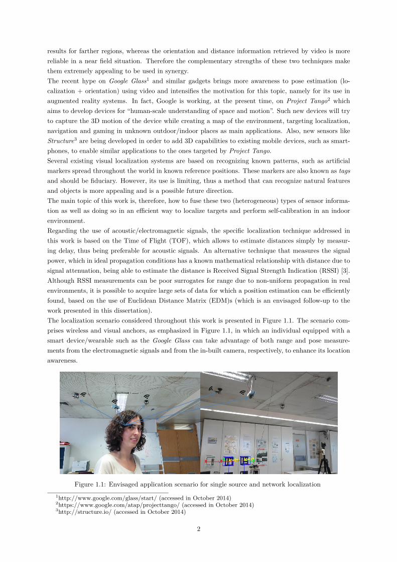
results for farther regions, whereas the orientation and distance information retrieved by video is morereliable in a near field situation. Therefore the complementary strengths of these two techniques makethem extremely appealing to be used in synergy.The recent hype on Google Glass1 and similar gadgets brings more awareness to pose estimation (lo-calization + orientation) using video and intensifies the motivation for this topic, namely for its use inaugmented reality systems. In fact, Google is working, at the present time, on Project Tango2 whichaims to develop devices for “human-scale understanding of space and motion”. Such new devices will tryto capture the 3D motion of the device while creating a map of the environment, targeting localization,navigation and gaming in unknown outdoor/indoor places as main applications. Also, new sensors likeStructure3 are being developed in order to add 3D capabilities to existing mobile devices, such as smart-phones, to enable similar applications to the ones targeted by Project Tango.Several existing visual localization systems are based on recognizing known patterns, such as artificialmarkers spread throughout the world in known reference positions. These markers are also known as tagsand should be fiduciary. However, its use is limiting, thus a method that can recognize natural featuresand objects is more appealing and is a possible future direction.The main topic of this work is, therefore, how to fuse these two (heterogeneous) types of sensor informa-tion as well as doing so in an efficient way to localize targets and perform self-calibration in an indoorenvironment.Regarding the use of acoustic/electromagnetic signals, the specific localization technique addressed inthis work is based on the Time of Flight (TOF), which allows to estimate distances simply by measur-ing delay, thus being preferable for acoustic signals. An alternative technique that measures the signalpower, which in ideal propagation conditions has a known mathematical relationship with distance due tosignal attenuation, being able to estimate the distance is Received Signal Strength Indication (RSSI) [3].Although RSSI measurements can be poor surrogates for range due to non-uniform propagation in realenvironments, it is possible to acquire large sets of data for which a position estimation can be efficientlyfound, based on the use of Euclidean Distance Matrix (EDM)s (which is an envisaged follow-up to thework presented in this dissertation).The localization scenario considered throughout this work is presented in Figure 1.1. The scenario com-prises wireless and visual anchors, as emphasized in Figure 1.1, in which an individual equipped with asmart device/wearable such as the Google Glass can take advantage of both range and pose measure-ments from the electromagnetic signals and from the in-built camera, respectively, to enhance its locationawareness.

Figure 1.1: Envisaged application scenario for single source and network localization1http://www.google.com/glass/start/ (accessed in October 2014)2https://www.google.com/atap/projecttango/ (accessed in October 2014)3http://structure.io/ (accessed in October 2014)

2

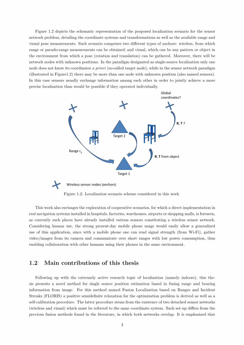
Figure 1.2 depicts the schematic representation of the proposed localization scenario for the sensornetwork problem, detailing the coordinate systems and transformations as well as the available range andvisual pose measurements. Such scenario comprises two different types of anchors: wireless, from whichrange or pseudo-range measurements can be obtained; and visual, which can be any pattern or object inthe environment from which a pose (rotation and translation) can be gathered. Moreover, there will benetwork nodes with unknown positions. In the paradigm designated as single-source localization only onenode does not know its coordinates a priori (so-called target node), while in the sensor network paradigm(illustrated in Figure1.2) there may be more than one node with unknown position (also named sensors).In this case sensors usually exchange information among each other in order to jointly achieve a moreprecise localization than would be possible if they operated individually.

R, T from object

Range rij

R, T ?

Global

coordinates?

Target 1

Wireless sensor nodes (anchors)

Target 2

Figure 1.2: Localization scenario scheme considered in this work

This work also envisages the exploration of cooperative scenarios, for which a direct implementation inreal navigation systems installed in hospitals, factories, warehouses, airports or shopping malls, is foreseen,as currently such places have already installed various sensors constituting a wireless sensor network.Considering human use, the strong present-day mobile phone usage would easily allow a generalizeduse of this application, since with a mobile phone one can read signal strength (from Wi-Fi), gathervideo/images from its camera and communicate over short ranges with low power consumption, thusenabling collaboration with other humans using their phones in the same environment.

1.2 Main contributions of this thesis

Following up with the extremely active research topic of localization (namely indoors), this the-sis presents a novel method for single source position estimation based in fusing range and bearinginformation from image. For this method named Fusion Localization based on Ranges and IncidentStreaks (FLORIS) a positive semidefinite relaxation for the optimization problem is derived as well as aself-calibration procedure. The latter procedure stems from the existence of two detached sensor networks(wireless and visual) which must be referred to the same coordinate system. Such set-up differs from theprevious fusion methods found in the literature, in which both networks overlap. It is emphasized that

3

such self-calibration procedure has no precedents in the author’s knowledge and is capable of calibratingthe networks without any a priori information, besides the wireless anchors coordinates.The proposed method is fully tested with numerical and practical experiments, revealing promising re-sults in both cases. In fact, it is shown that the new hybrid method outperforms, numerically, otherlocalization methods, specially when the measurements are quite noisy. Although several physical set-backs were found, when tested in an experimental set-up, the majority was surpassed, paving the way todemonstrate the validity of the new method in a real scenario. Hence, the new method is fully developed,implemented and tested in this dissertation work, which in addition to the auspicious attained resultsembodies an important contribution.Moreover, the work related to the single-source paradigm (FLORIS method) is included in the paper “Aunified framework for Hybrid Source Localization based on ranges and video”, submitted to the IEEEInternational Conference on Acoustics, Speech and Signal Processing (ICASSP) 2015.After tackling the single source localization, the sensor network localization problem is also addressed.This paradigm proves to be even more challenging, as fused measurements from multiple targets mustbe combined so that the position estimation is enhanced. Nevertheless, a new algorithm (CollaborativeLocalization based on Ranges and Incident Streaks (CLORIS)) based on a disk relaxation method fusingboth range and streaks measurements is devised. The latter algorithm is also tested both in simulationand in a real application scenario, achieving very good results (both in accuracy and execution time).It should be noted that in the experimental scenario, the fusion scheme outperforms the single-sensedvariable approach. Hence, the introduced solution for the sensor network problem is another relevantcontribution of this dissertation to this field of work.

1.3 Outline

The remainder of this dissertation is organized as follows: in Chapter 2 the state-of-the-art relevantto this work is addressed and discussed; Chapter 3 describes the approaches developed and followed inorder to achieve the various proposed goals, namely introducing the new derived algorithms (single-sourceand cooperative) and procedures (self-calibration) to perform hybrid localization; in Chapter 4 extensivesimulation and experimental results regarding performance are presented and compared with other state-of-the art methods. Finally, Chapter 5 states the conclusions of this thesis, pointing also some futureresearch work directions and further improvements.

4

Chapter 2

Related Work

This Chapter provides an overview of the state-of-the-art related to the problems addressed in thisthesis. The main theme is localization, and work associated with range-based positioning, vision, opti-mization and classification methods is discussed. The remainder of this Chapter is organized in a majorSection about Localization 2.1, which is divided into Ranges and Vision approaches. Inside Range Sub-section 2.1.1, the optimization based single-source localization methods are addressed and then a specialfocus on the use of Euclidean Distance Matrices to solve localization in a collaborative paradigm is made.Throughout the Vision Subsection 2.1.2, several methods that are found to be useful tools for localizationare discussed. The last Subsection addresses the previous work found in the literature that deals withthe same topic as this work, namely, fusion of sensor data to perform localization.

NotationThroughout this document, both scalars and individual position vectors will be represented by lower-caseletters. Vectors of concatenated coordinates and matrices will be denoted by boldface lower-case andupper-case, respectively. The superscript ∗ stands for the conjugate transpose and T for the transposeof the given real vector or matrix. Im is the identity matrix with dimension m×m and 1m the vector ofm ones. For symmetric matrix X, X � 0 means that X is positive semidefinite.

2.1 Localization

According to Bachrach and Taylor [3], nowadays ad-hoc sensor networks present new trade-offs insystem design, as they use very inexpensive nodes rather than globally accessible beacons or GPS. Thesesensor networks should self define a coordinate system and have enabled emerging applications such ashabitat monitoring, smart building failure detection or target tracking. Additionally, GPS is not a validalternative, for example to be used indoors since the satellite links are blocked or unreadable insidebuildings [29]. There are several localization schemes, hardware architectures and methods [3, 44]; in thiswork only a small part shall be addressed. The diagram in Figure 2.1 shows relevant aspects in localizationsystems such as the network scheme, ranging methods, computational organization, localization methodsand algorithms, based on [3, 35] .Concerning the hardware implementation, an architecture with anchors (also called beacon nodes), whichare simple sensor nodes, is recurrent. These anchors can define relative physical coordinates, known a

5

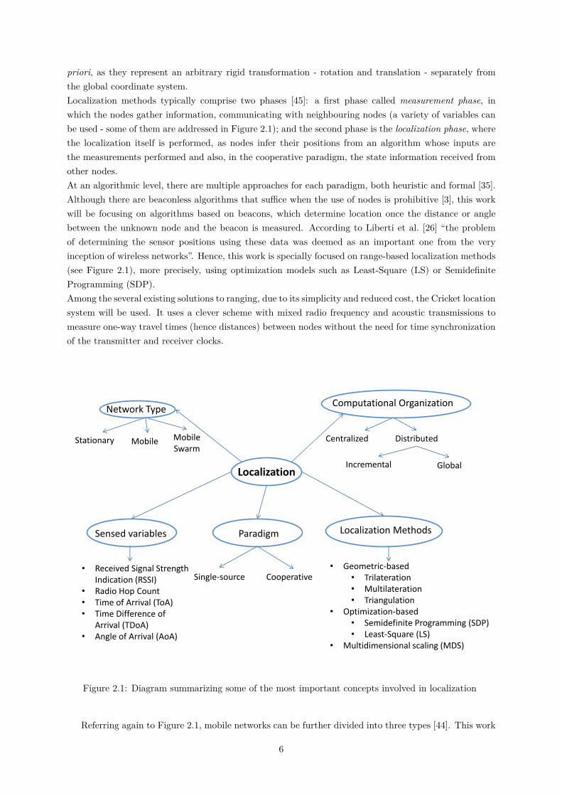
priori, as they represent an arbitrary rigid transformation - rotation and translation - separately fromthe global coordinate system.Localization methods typically comprise two phases [45]: a first phase called measurement phase, inwhich the nodes gather information, communicating with neighbouring nodes (a variety of variables canbe used - some of them are addressed in Figure 2.1); and the second phase is the localization phase, wherethe localization itself is performed, as nodes infer their positions from an algorithm whose inputs arethe measurements performed and also, in the cooperative paradigm, the state information received fromother nodes.At an algorithmic level, there are multiple approaches for each paradigm, both heuristic and formal [35].Although there are beaconless algorithms that suffice when the use of nodes is prohibitive [3], this workwill be focusing on algorithms based on beacons, which determine location once the distance or anglebetween the unknown node and the beacon is measured. According to Liberti et al. [26] “the problemof determining the sensor positions using these data was deemed as an important one from the veryinception of wireless networks”. Hence, this work is specially focused on range-based localization methods(see Figure 2.1), more precisely, using optimization models such as Least-Square (LS) or SemidefiniteProgramming (SDP).Among the several existing solutions to ranging, due to its simplicity and reduced cost, the Cricket locationsystem will be used. It uses a clever scheme with mixed radio frequency and acoustic transmissions tomeasure one-way travel times (hence distances) between nodes without the need for time synchronizationof the transmitter and receiver clocks.

Localization

Network Type

Stationary Mobile Mobile Swarm

Computational Organization

Centralized Distributed

Sensed variables

• Received Signal Strength Indication (RSSI)

• Radio Hop Count • Time of Arrival (ToA) • Time Difference of

Arrival (TDoA) • Angle of Arrival (AoA)

Localization Methods

• Geometric-based • Trilateration • Multilateration • Triangulation

• Optimization-based • Semidefinite Programming (SDP) • Least-Square (LS)

• Multidimensional scaling (MDS)

Incremental Global

Paradigm

Single-source Cooperative

Figure 2.1: Diagram summarizing some of the most important concepts involved in localization

Referring again to Figure 2.1, mobile networks can be further divided into three types [44]. This work

6

will consider the mobile scheme type where the unknown nodes are moving while the anchors are static.Furthermore, in a non-cooperative sensor network, source nodes (or targets) can communicate only withanchor nodes, whereas in a cooperative localization paradigm source nodes are able to communicate withboth anchor nodes and other targets [31], improving the accuracy of location information [45].A few algorithms used for localization for stationary networks are [44]: Simultaneous Localization andSynchronization (L-S), Large-Scale Hierarchical Localization (LSHL) and Three-Dimensional Underwa-ter Localization (3DUL), where the last two are applied to underwater scenarios. Regarding mobilenetworks, algorithms that rely on prior information, allowing localization to benefit from knowledge ofthe dynamics for improved efficiency and accuracy, are frequently used [44], such as the Monte CarloLocalization (MCL), Scalable Localization with Mobility Prediction (SLMP), Simultaneous Localizationand Environmental Mapping (SLAM). These prediction based algorithms determine the current locationby integrating the prediction from the prior information (prediction phase) with the measurement up-date from the environment observation (update phase). Filtering methods such as the Extended KalmanFilter (EKF) or Markov methods are usually applied [44]. As for mobile swarm networks, a schemein which both unknown nodes and beacons are moving (usual in ocean environments) presents severaladvantages like enhanced coverage and flexibility, efficiency and suitability for cooperation [44]. Someof the algorithms applied are: Motion-Aware Self Localization (MASL), Collaborative Localization (CL)and also Monte Carlo Localization (MCL).Finally, included in the category of centralized algorithms we may find SDP or MDS [3], whilst in thedistributed case algorithms such as Diffusion, Bounding Box or Gradient are used [3]. The design of suchlocalization algorithms has commonly constraints in resources [3], since usually nodes have to be smalland cheap. Such restraints have lead to the development of systems characterized by weak processing,sensing and communication capabilities.In the following Subsections, some algorithms resorting to both distance measurements between nearbysensor nodes and pose estimation of a target will be addressed in further detail. More specifically, wewill focus on optimization based methods rather than ad-hoc approaches. The previous methods are in-trinsically more robust when dealing with noisy measurements, which is frequent in the low-cost rangingsystems that are of interest to this work.

2.1.1 Range

One of the more commonly used types of measurement is range. The measurement phase suffersfrom several impairments such as noise, multipath blockages, signal interferences, clock drifts and otherenvironmental effects [45]. Thus choosing the adequate subjacent measurement technique is pivotal.Range can be directly obtained from Time of Arrival (ToA) and Time Difference of Arrival, which com-prise two of the most straightforward methods to sense this variable. In fact, the ranges obtained in theexperimental part of this work are computed through the ToA of electromagnetic and acoustic signals,knowing the propagation velocities.Among the other techniques to compute range information, RSSI is based on the way that the energy ofa radio signal decreases with distance (following an inverse square law in free space) from the source [3].Thus, RSSI measurement model is a function of the transmit power of the source node. Knowing thisfunction of magnitude that depends on the distance and the reported power transmitted at the origin, anode listening to a radio transmission should be able to use the strength of the received signal to calculatethe range (from the transmitter). Yet, RSSI shows, in practice, some disadvantages, because its rangingmeasurements are quite noisy (on the order of several meters) leading to uncertainty, as radio propagationtends to be highly non-uniform in real environments (walls and objects reflect and absorb radio waves).

7

Nonetheless, RSSI is an attractive method mainly because of its low hardware complexity and cost [31].

2.1.1.1 Single-Source Localization Problems - optimization based methods

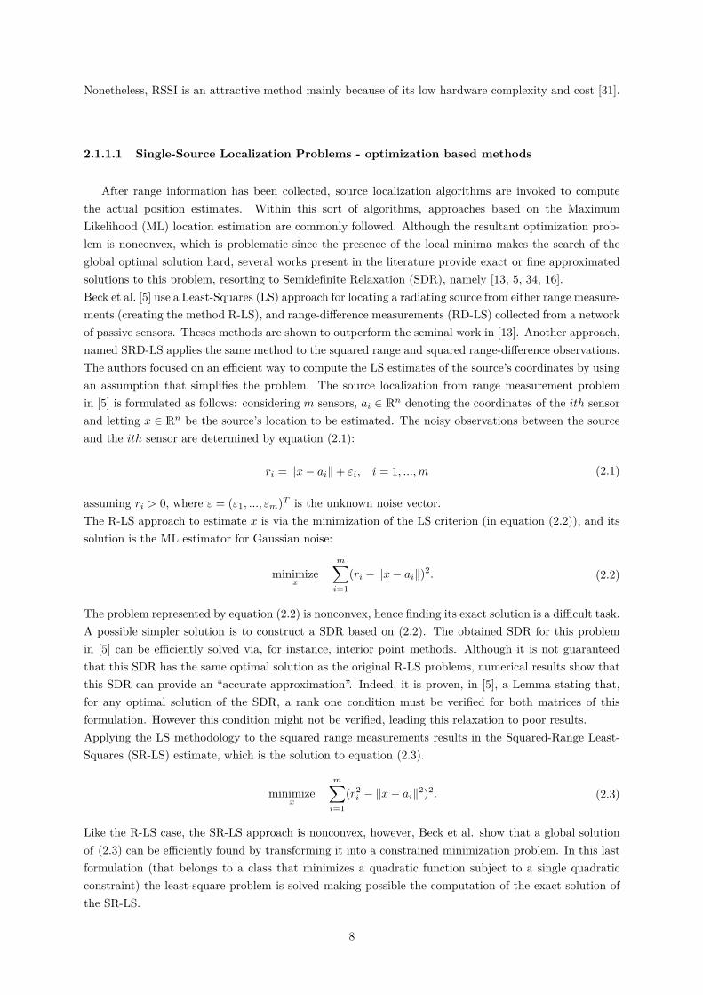
After range information has been collected, source localization algorithms are invoked to computethe actual position estimates. Within this sort of algorithms, approaches based on the MaximumLikelihood (ML) location estimation are commonly followed. Although the resultant optimization prob-lem is nonconvex, which is problematic since the presence of the local minima makes the search of theglobal optimal solution hard, several works present in the literature provide exact or fine approximatedsolutions to this problem, resorting to Semidefinite Relaxation (SDR), namely [13, 5, 34, 16].Beck et al. [5] use a Least-Squares (LS) approach for locating a radiating source from either range measure-ments (creating the method R-LS), and range-difference measurements (RD-LS) collected from a networkof passive sensors. Theses methods are shown to outperform the seminal work in [13]. Another approach,named SRD-LS applies the same method to the squared range and squared range-difference observations.The authors focused on an efficient way to compute the LS estimates of the source’s coordinates by usingan assumption that simplifies the problem. The source localization from range measurement problemin [5] is formulated as follows: considering m sensors, ai ∈ Rn denoting the coordinates of the ith sensorand letting x ∈ Rn be the source’s location to be estimated. The noisy observations between the sourceand the ith sensor are determined by equation (2.1):

ri = ‖x− ai‖+ εi, i = 1, ...,m (2.1)

assuming ri > 0, where ε = (ε1, ..., εm)T is the unknown noise vector.The R-LS approach to estimate x is via the minimization of the LS criterion (in equation (2.2)), and itssolution is the ML estimator for Gaussian noise:

minimizex

m∑i=1

(ri − ‖x− ai‖)2. (2.2)

The problem represented by equation (2.2) is nonconvex, hence finding its exact solution is a difficult task.A possible simpler solution is to construct a SDR based on (2.2). The obtained SDR for this problemin [5] can be efficiently solved via, for instance, interior point methods. Although it is not guaranteedthat this SDR has the same optimal solution as the original R-LS problems, numerical results show thatthis SDR can provide an “accurate approximation”. Indeed, it is proven, in [5], a Lemma stating that,for any optimal solution of the SDR, a rank one condition must be verified for both matrices of thisformulation. However this condition might not be verified, leading this relaxation to poor results.Applying the LS methodology to the squared range measurements results in the Squared-Range Least-Squares (SR-LS) estimate, which is the solution to equation (2.3).

minimizex

m∑i=1

(r2i − ‖x− ai‖2)2. (2.3)

Like the R-LS case, the SR-LS approach is nonconvex, however, Beck et al. show that a global solutionof (2.3) can be efficiently found by transforming it into a constrained minimization problem. In this lastformulation (that belongs to a class that minimizes a quadratic function subject to a single quadraticconstraint) the least-square problem is solved making possible the computation of the exact solution ofthe SR-LS.

8

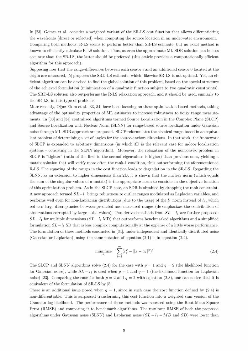
In [23], Gomes et al. consider a weighted variant of the SR-LS cost function that allows differentiatingthe wavefronts (direct or reflected) when computing the source location in an underwater environment.Comparing both methods, R-LS seems to perform better than SR-LS estimate, but no exact method isknown to efficiently calculate R-LS solution. Thus, as even the approximate ML-SDR solution can be lessaccurate than the SR-LS, the latter should be preferred (this article provides a computationally efficientalgorithm for this approach).Supposing now that the range-differences between each sensor i and an additional sensor 0 located at theorigin are measured, [5] proposes the SRD-LS estimate, which, likewise SR-LS is not optimal. Yet, an ef-ficient algorithm can be devised to find the global solution of this problem, based on the special structureof the achieved formulation (minimization of a quadratic function subject to two quadratic constraints).The SRD-LS solution also outperforms the R-LS relaxation approach, and it should be used, similarly tothe SR-LS, in this type of problems.More recently, Oguz-Ekim et al. [33, 34] have been focusing on these optimization-based methods, takingadvantage of the optimality properties of ML estimates to increase robustness to noisy range measure-ments. In [33] and [34] centralized algorithms termed Source Localization in the Complex Plane (SLCP)and Source Localization with Nuclear Norm (SLNN) for range-based source localization under Gaussiannoise through ML-SDR approach are proposed. SLCP reformulates the classical range-based in an equiva-lent problem of determining a set of angles for the source-anchors directions. In that work, the frameworkof SLCP is expanded to arbitrary dimensions (in which 3D is the relevant case for indoor localizationsystems - consisting in the SLNN algorithm). Moreover, the relaxation of the nonconvex problem inSLCP is “tighter” (ratio of the first to the second eigenvalues is higher) than previous ones, yielding amatrix solution that will verify more often the rank-1 condition, thus outperforming the aforementionedR-LS. The squaring of the ranges in the cost function leads to degradation in the SR-LS. Regarding theSLNN, as an extension to higher dimensions than 2D, it is shown that the nuclear norm (which equalsthe sum of the singular values of a matrix) is the appropriate norm to consider in the objective functionof this optimization problem. As in the SLCP case, an SDR is obtained by dropping the rank constraint.A new approach termed SL−l1 brings robustness to outlier ranges modulated as Laplacian variables, andperforms well even for non-Laplacian distributions, due to the usage of the l1 norm instead of l2, whichreduces large discrepancies between predicted and measured ranges (de-emphasizes the contribution ofobservations corrupted by large noise values). Two derived methods from SL− l1 are further proposed:SL− l1 for multiple dimensions (SL− l1 MD) that outperforms benchmarked algorithms and a simplifiedformulation SL− l1 SD that is less complex computationally at the expense of a little worse performance.The formulation of these methods conducted in [34], under independent and identically distributed noise(Gaussian or Laplacian), using the same notation of equation (2.1) is in equation (2.4).

minimizex

m∑i=1

(rpi − ‖x− ai‖p)q (2.4)

The SLCP and SLNN algorithms solve (2.4) for the case with p = 1 and q = 2 (the likelihood functionfor Gaussian noise), while SL − l1 is used when p = 1 and q = 1 (the likelihood function for Laplaciannoise) [23]. Comparing the case for both p = 2 and q = 2 with equation (2.3), one can notice that it isequivalent of the formulation of SR-LS by [5].There is an additional issue posed when q = 1, since in such case the cost function defined by (2.4) isnon-differentiable. This is surpassed transforming this cost function into a weighted sum version of theGaussian log-likelihood. The performance of these methods was assessed using the Root-Mean-SquareError (RMSE) and comparing it to benchmark algorithms. The resultant RMSE of both the proposedalgorithms under Gaussian noise (SLNN) and Laplacian noise (SL− l1 −MD and SD) were lower than

9

all the existing methods, the latter specially in the presence of outliers.The convexity and tightness of SLCP is also evaluated, and it is found out, by simulation results, thatthe convexity as well as the tightness of SLCP is superior to the previous SDR. Results seem to indicatethat this convexity behaviour is mostly because SLCP has a higher probability of having a solution withrank near 1.

2.1.1.2 Cooperative Localization Paradigm - optimization based methods

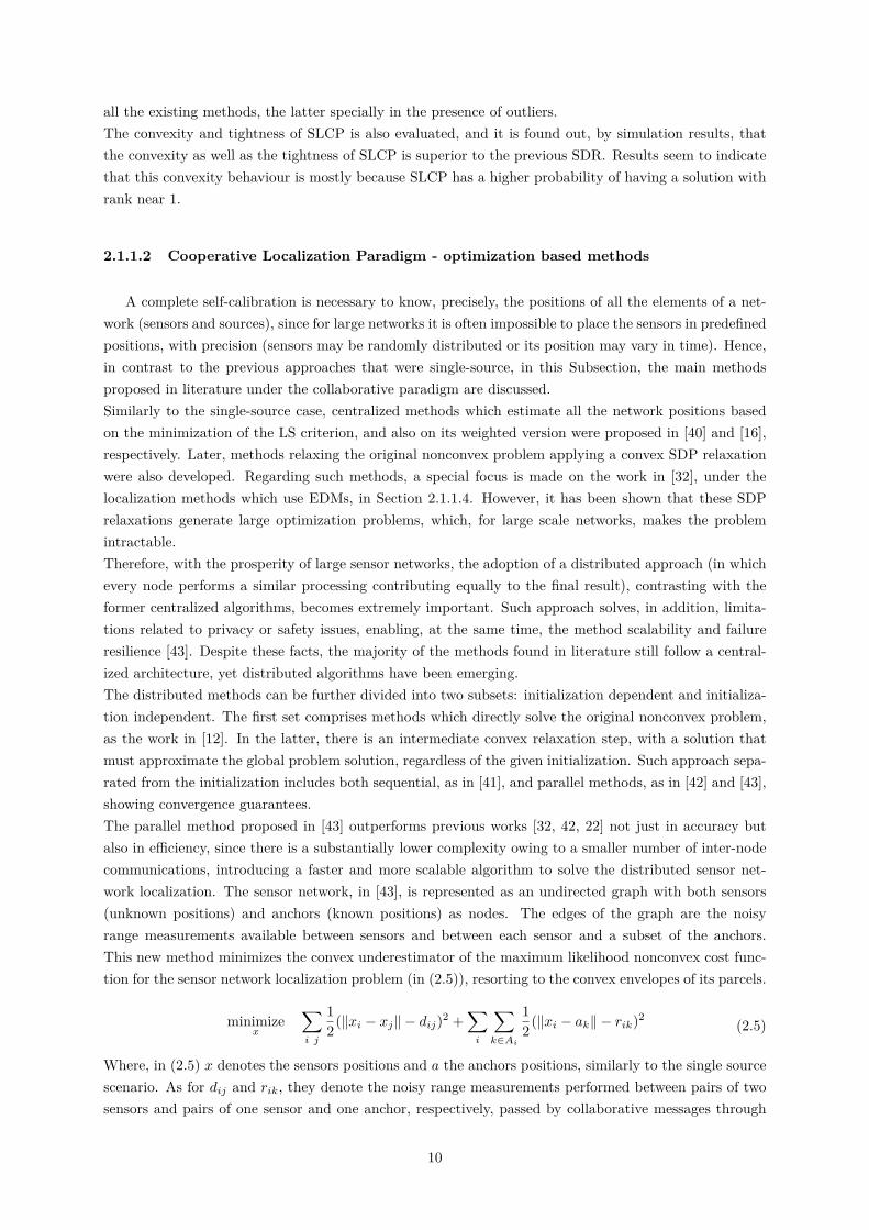
A complete self-calibration is necessary to know, precisely, the positions of all the elements of a net-work (sensors and sources), since for large networks it is often impossible to place the sensors in predefinedpositions, with precision (sensors may be randomly distributed or its position may vary in time). Hence,in contrast to the previous approaches that were single-source, in this Subsection, the main methodsproposed in literature under the collaborative paradigm are discussed.Similarly to the single-source case, centralized methods which estimate all the network positions basedon the minimization of the LS criterion, and also on its weighted version were proposed in [40] and [16],respectively. Later, methods relaxing the original nonconvex problem applying a convex SDP relaxationwere also developed. Regarding such methods, a special focus is made on the work in [32], under thelocalization methods which use EDMs, in Section 2.1.1.4. However, it has been shown that these SDPrelaxations generate large optimization problems, which, for large scale networks, makes the problemintractable.Therefore, with the prosperity of large sensor networks, the adoption of a distributed approach (in whichevery node performs a similar processing contributing equally to the final result), contrasting with theformer centralized algorithms, becomes extremely important. Such approach solves, in addition, limita-tions related to privacy or safety issues, enabling, at the same time, the method scalability and failureresilience [43]. Despite these facts, the majority of the methods found in literature still follow a central-ized architecture, yet distributed algorithms have been emerging.The distributed methods can be further divided into two subsets: initialization dependent and initializa-tion independent. The first set comprises methods which directly solve the original nonconvex problem,as the work in [12]. In the latter, there is an intermediate convex relaxation step, with a solution thatmust approximate the global problem solution, regardless of the given initialization. Such approach sepa-rated from the initialization includes both sequential, as in [41], and parallel methods, as in [42] and [43],showing convergence guarantees.The parallel method proposed in [43] outperforms previous works [32, 42, 22] not just in accuracy butalso in efficiency, since there is a substantially lower complexity owing to a smaller number of inter-nodecommunications, introducing a faster and more scalable algorithm to solve the distributed sensor net-work localization. The sensor network, in [43], is represented as an undirected graph with both sensors(unknown positions) and anchors (known positions) as nodes. The edges of the graph are the noisyrange measurements available between sensors and between each sensor and a subset of the anchors.This new method minimizes the convex underestimator of the maximum likelihood nonconvex cost func-tion for the sensor network localization problem (in (2.5)), resorting to the convex envelopes of its parcels.

minimizex

∑i j

12(‖xi − xj‖ − dij)2 +

∑i

∑k∈Ai

12(‖xi − ak‖ − rik)2

(2.5)

Where, in (2.5) x denotes the sensors positions and a the anchors positions, similarly to the single sourcescenario. As for dij and rik, they denote the noisy range measurements performed between pairs of twosensors and pairs of one sensor and one anchor, respectively, passed by collaborative messages through

10

neighbouring nodes.

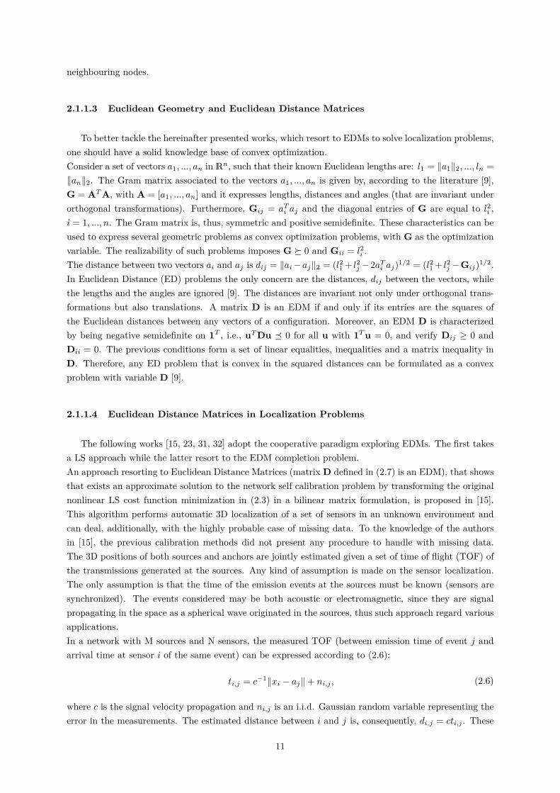
2.1.1.3 Euclidean Geometry and Euclidean Distance Matrices

To better tackle the hereinafter presented works, which resort to EDMs to solve localization problems,one should have a solid knowledge base of convex optimization.Consider a set of vectors a1, ..., an in Rn, such that their known Euclidean lengths are: l1 = ‖a1‖2, ..., ln =‖an‖2. The Gram matrix associated to the vectors a1, ..., an is given by, according to the literature [9],G = ATA, with A = [a1, ..., an] and it expresses lengths, distances and angles (that are invariant underorthogonal transformations). Furthermore, Gij = aTi aj and the diagonal entries of G are equal to l2i ,i = 1, ..., n. The Gram matrix is, thus, symmetric and positive semidefinite. These characteristics can beused to express several geometric problems as convex optimization problems, with G as the optimizationvariable. The realizability of such problems imposes G � 0 and Gii = l2i .

The distance between two vectors ai and aj is dij = ‖ai−aj‖2 = (l21 + l2j −2aTi aj)1/2 = (l21 + l2j −Gij)1/2.

In Euclidean Distance (ED) problems the only concern are the distances, dij between the vectors, whilethe lengths and the angles are ignored [9]. The distances are invariant not only under orthogonal trans-formations but also translations. A matrix D is an EDM if and only if its entries are the squares ofthe Euclidean distances between any vectors of a configuration. Moreover, an EDM D is characterizedby being negative semidefinite on 1T , i.e., uTDu � 0 for all u with 1Tu = 0, and verify Dij ≥ 0 andDii = 0. The previous conditions form a set of linear equalities, inequalities and a matrix inequality inD. Therefore, any ED problem that is convex in the squared distances can be formulated as a convexproblem with variable D [9].

2.1.1.4 Euclidean Distance Matrices in Localization Problems

The following works [15, 23, 31, 32] adopt the cooperative paradigm exploring EDMs. The first takesa LS approach while the latter resort to the EDM completion problem.An approach resorting to Euclidean Distance Matrices (matrix D defined in (2.7) is an EDM), that showsthat exists an approximate solution to the network self calibration problem by transforming the originalnonlinear LS cost function minimization in (2.3) in a bilinear matrix formulation, is proposed in [15].This algorithm performs automatic 3D localization of a set of sensors in an unknown environment andcan deal, additionally, with the highly probable case of missing data. To the knowledge of the authorsin [15], the previous calibration methods did not present any procedure to handle with missing data.The 3D positions of both sources and anchors are jointly estimated given a set of time of flight (TOF) ofthe transmissions generated at the sources. Any kind of assumption is made on the sensor localization.The only assumption is that the time of the emission events at the sources must be known (sensors aresynchronized). The events considered may be both acoustic or electromagnetic, since they are signalpropagating in the space as a spherical wave originated in the sources, thus such approach regard variousapplications.In a network with M sources and N sensors, the measured TOF (between emission time of event j andarrival time at sensor i of the same event) can be expressed according to (2.6):

ti,j = c−1‖xi − aj‖+ ni,j , (2.6)

where c is the signal velocity propagation and ni,j is an i.i.d. Gaussian random variable representing theerror in the measurements. The estimated distance between i and j is, consequently, di,j = cti,j . These

11

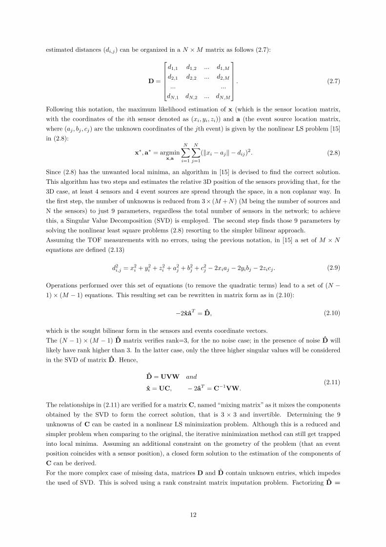
estimated distances (di,j) can be organized in a N ×M matrix as follows (2.7):

D =

d1,1 d1,2 ... d1,M

d2,1 d2,2 ... d2,M

... ...

dN,1 dN,2 ... dN,M

. (2.7)

Following this notation, the maximum likelihood estimation of x (which is the sensor location matrix,with the coordinates of the ith sensor denoted as (xi, yi, zi)) and a (the event source location matrix,where (aj , bj , cj) are the unknown coordinates of the jth event) is given by the nonlinear LS problem [15]in (2.8):

x∗,a∗ = argminx,a

N∑i=1

N∑j=1

(‖xi − aj‖ − dij)2. (2.8)

Since (2.8) has the unwanted local minima, an algorithm in [15] is devised to find the correct solution.This algorithm has two steps and estimates the relative 3D position of the sensors providing that, for the3D case, at least 4 sensors and 4 event sources are spread through the space, in a non coplanar way. Inthe first step, the number of unknowns is reduced from 3× (M +N) (M being the number of sources andN the sensors) to just 9 parameters, regardless the total number of sensors in the network; to achievethis, a Singular Value Decomposition (SVD) is employed. The second step finds those 9 parameters bysolving the nonlinear least square problems (2.8) resorting to the simpler bilinear approach.Assuming the TOF measurements with no errors, using the previous notation, in [15] a set of M × Nequations are defined (2.13)

d2i,j = x2

i + y2i + z2

i + a2j + b2j + c2j − 2xiaj − 2yibj − 2zicj . (2.9)

Operations performed over this set of equations (to remove the quadratic terms) lead to a set of (N −1)× (M − 1) equations. This resulting set can be rewritten in matrix form as in (2.10):

−2xaT = D, (2.10)

which is the sought bilinear form in the sensors and events coordinate vectors.The (N − 1) × (M − 1) D matrix verifies rank=3, for the no noise case; in the presence of noise D willlikely have rank higher than 3. In the latter case, only the three higher singular values will be consideredin the SVD of matrix D. Hence,

D = UVW and

x = UC, − 2aT = C−1VW.(2.11)

The relationships in (2.11) are verified for a matrix C, named “mixing matrix” as it mixes the componentsobtained by the SVD to form the correct solution, that is 3 × 3 and invertible. Determining the 9unknowns of C can be casted in a nonlinear LS minimization problem. Although this is a reduced andsimpler problem when comparing to the original, the iterative minimization method can still get trappedinto local minima. Assuming an additional constraint on the geometry of the problem (that an eventposition coincides with a sensor position), a closed form solution to the estimation of the components ofC can be derived.For the more complex case of missing data, matrices D and D contain unknown entries, which impedesthe used of SVD. This is solved using a rank constraint matrix imputation problem. Factorizing D =

12

FG and defining the variable m for the missing entries, the following optimization problem is obtained:

minimize ‖D(m)− FG‖2. (2.12)

An iterative algorithm to solve (2.12) is presented. This algorithm is said to be general to the numerouscontexts in which rank constraint matrix imputation problems are involved. Moreover, this procedureshows similarities with the power factorization method used for the Structure from Motion topic (as isdiscussed in Subsection 2.1.2 Vision). Once matrices F and G are determined, the coefficients of themixing matrix C are found with the same procedure explained in the non missing data situation.

A Wireless Sensor Network Localization (WSNL) is said to be solvable if it has a unique valid realiza-tion, also known as global rigidity [26]. The network anchors play a pivotal role, as they ensure the globalrigidity in RK , thus the set of anchors should have K + 1 or more elements. These facts are the basis forthe exploration of SDP to solve EDM completion problems, addressed in the next articles [23, 31, 32],since such relaxation is fundamental as low-dimensional EDM completion is NP-hard [24].The established methods for determining the positions of sensor nodes and a moving target in a network(SLAT problem) are based on ML function, as described in the previous Subsection. However, such meth-ods require an initialization with an approximate solution in order to avoid getting trapped in the localminima. Since in sensor network localization (SNL) it is frequent that the positions of several nodes haveto be simultaneously computed from pairwise range measurements, Euclidean Distance Matrices providea suitable and elegant framework for this topic [23]. Oguz-Ekim et al. in [32] propose a centralized local-ization method that uses incomplete and noisy (both Gaussian and Laplacian) range measurements, andis based on a modified EDM completion problem and SDP, and not in a Bayesian framework as [20] (inwhich bearing information is estimated from camera images - see Subsection 2.1.2 Vision). Once solvedthe completion problem for a block of range measurements, thus finding the initial sensor and targetpositions, the likelihood function is iteratively improved through Majorization-Minimization (MM). Also,a scheme, in which the current target/node position is estimated from previous locations, is developedto avoid solving the larger EDMs with time. More specifically, it is proposed a two stage algorithmcomposed by a startup and update phases. Startup phase main goal is to obtain an outline of the networkconfiguration from a batch of measurements, whereas in the update phase new target observations areincrementally treated as they become available, improving also all previous determined locations. Bothphases include, in its turn, initialization and refinement steps. The first calculates approximate locations(in startup it is solved an EDM completion problem while in update it is solved a source localization prob-lem) whilst the second is an iterative step using MM to refine the likelihood function. Besides solving theSLAT problem with modest prior knowledge on target/sensor positions with moderate complexity, [32]uses cost functions with plain ranges (non-squared) which improves robustness in the case of high noise.Suitable cost functions are derived for Gaussian and Laplacian noise, being more robust, in both cases,than standard EDM methods, due to the use of plain ranges. Under Gaussian noise in the update phaseit is used the SLCP time-recursive method, under Laplacian noise the SL− l1 is applied.Focusing on the EDM problem formulation with squared ranges, a D matrix (denominated pre-distancematrix) with elements Dij = d2

ij and diagonal entries zero is used to find an EDM E (satisfyingEij = ‖yi − yj‖2) that is nearest to D, in the LS sense. Thus, for 2D, this problem is formulated

13

according to equation (2.13) [32]:

minimizeE

∑i,j∈O

(Eij − dij)2

subject to E ∈ EDM, E(A) = A

rank(JEJ) = 2,

(2.13)

where J = (Iρ − 1ρ1ρ1Tρ ) is a centering operator and ρ = m+ n+ l (m is the number of unknown target

positions, n of unknown sensors and l of anchors) and O is the index set for which range measurementsare available. Matrix E should satisfy the properties listed in the previous Subsection. And the rankconstraint guarantees that the solution is compatible with a configuration of sensor/anchor/targets inR2. Furthermore, A is the index set of anchor distances and Aij = ‖ai− aj‖2 is the corresponding EDMsubmatrix that enforces the a priori information. A convex SDP compact relaxed formulation (since therank constraint is ignored), in matrix notation, is presented in (2.14) and is called EDM with squaredranges

minimizeE

‖W� (E−D)‖2F

subject to E ∈ EDM, E(A) = A,(2.14)

where W is a mask matrix having zero entries in the free elements of D.A similar process is performed for the plain ranges case, obtaining the EDM completion formulation in(2.15)

minimizeE

∑i,j

(√

Eij − dij)2

subject to E ∈ EDM, E(A) = A

rank(JEJ) = 2,

(2.15)

and the relaxed SDP (obtained using the epigraph technique, introducing variable T and dropping, again,the rank constraint) in (2.16)

minimizeE, T

∑i,j

(Eij − 2Tijdij)

subject to T2ij ≤ Eij ,

E ∈ EDM, E(A) = A.

(2.16)

Since the solution of these problems is a distance matrix, the Gram matrix should be obtained (factorizing-JEJ) to, afterwards, extract the node coordinates by SVD [24] and solving a Procrustes problem.Simulation results show that these methods are more robust to outliers than existing ones and are runreasonably fast for small networks (about 30 unknown positions). Even further, for small Gaussian noise,the Cramer-Rao lower bound is almost achieved.Convex formulations (2.15) and (2.16) are equally applied in the underwater scenario, by Gomes et al.in [23], for which a solution in simulation, for a network with approximately 50 nodes, is reliably found.In the experiments of [23], it was verified that the formulation (2.16) has better numerical propertiesthan (2.14), allowing the use of a faster solver.More recently, however, Soares et. al, in [43], propose an optimal distributed algorithm that outperformsprevious methods based on SDP and on edge-based relaxations. Furthermore the algorithm in [43] alsohas superior performance (both in accuracy and in communication volume) than the method based inEDM completion of [32].

14

2.1.2 Vision

This Section includes some relevant work on localization systems based on vision, namely using acamera network that follows a target in [20], mobile cameras that only recognize markers, whose locationsare known, in [29] or cameras recognizing tags in order to measure ranges and perform mapping in [38].Feature descriptors, such as the Scale-Invariant Feature Transform (SIFT) method from [27], have beenalso used in mapping and localization systems without targets or markers, thus recognizing objects ornatural features, in [18].Moreover, in parallel to localization based on video images, some important topics from the field of imageprocessing are discussed since they can be helpful tools to perform such image aided localization. Someliterature on these topics will be addressed afterwards, targeting on image recognition and reconstructionin [28] and image classification in [11].

Camera networks are perhaps the most common type of sensor network nowadays. However, a keyproblem in deploying such networks is their calibration, i.e., determining the location and orientationof each network sensor, so that the observations in an image can be mapped into locations in the realworld [20]. Furthermore, a camera pose can be represented by 6 parameters: 3 position parameters (X,Y, Z) and 3 angles (for example: roll, pitch, yaw), therefore the calibration procedure must recover theseparameters. The notation (X, Y, θ), where θ is the rotation around the z-axis, is known as the absoluteparametrization of a camera pose.For a network with a single type of sensor, Funiak et al. [20] proposed an approach for camera networkcalibration addressed by solving a localization and tracking (SLAT) problem, where both the trajectoryof a moving target and all the camera poses are estimated. In such problem, the cameras collaborate totrack a moving object through the environment, reasoning probabilistically (to handle the non-linearitiesof the projective transformation and the dense correlations arisen between distant sensors) about whichcamera poses are consistent with the observed images of this environment. Therefore, with cameras placedthroughout the environment at unknown locations, with an object moving accordingly to an unknown(smooth) trajectory, the network can automatically calibrate itself. The main contributions of such workare a novel representation (named relative over-parametrization - ROP) and hybrid conditional linearisa-tion techniques that enable the use of a single Gaussian variable to a Kalman Filter solution to the SLATproblem and a stable and online algorithm that converges always to the same solution as the centralizedapproach (contrary to the existing similar approaches that are off-line and centralized, such as [37]). Theauthors claim that the performance of their solution is very good, even when the communication is lossy,as it was experimented on a real camera network with 25 nodes, with relatively low link quality betweennodes (due to packet loss or interference), generating pose estimates within 90% confidence intervals.The proposed solution also obtains the respective uncertainty of each estimate.The approach used in [20] (SLAT) is related to SLAM, since SLAT can be understood as a SLAM prob-lem where the cameras are the landmarks (anchors) and the moving object plays the role of the robot.Some aspects of SLAT are related also to computer vision topic Structure from Motion (SFM), whichconsists in recovering the 3D geometry of a scene as well as the trajectory of the camera motion, makingcorrespondences between feature points. This is in the line with the 3D scene reconstruction from thou-sands of images, in [1], accomplished in an very efficient way, due to the use of novel parallel distributedmatching and reconstruction algorithms.More recently, triggered by the widespread and popularity of RGB-D cameras (a sensor which providesboth color images and dense depth maps), such as the Microsoft Kinect or Asus Xtion Pro, several newapproaches to SLAM algorithms have been proposed. In fact, in [18], a system that simultaneously gen-erates a dense 3D model of the surrounding environment and estimates the RGB-D camera pose (and

15

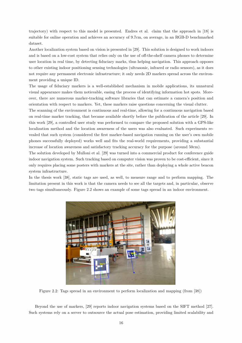
trajectory) with respect to this model is presented. Endres et al. claim that the approach in [18] issuitable for online operation and achieves an accuracy of 9.7cm, on average, in an RGB-D benchmarkeddataset.Another localization system based on vision is presented in [29]. This solution is designed to work indoorsand is based on a low-cost system that relies only on the use of off-the-shelf camera phones to determineuser location in real time, by detecting fiduciary marks, thus helping navigation. This approach opposesto other existing indoor positioning sensing technologies (ultrasonic, infrared or radio sensors), as it doesnot require any permanent electronic infrastructure; it only needs 2D markers spread across the environ-ment providing a unique ID.The usage of fiduciary markers is a well-established mechanism in mobile applications, its unnaturalvisual appearance makes them noticeable, easing the process of identifying information hot spots. More-over, there are numerous marker-tracking software libraries that can estimate a camera’s position andorientation with respect to markers. Yet, these markers raise questions concerning the visual clutter.The scanning of the environment is continuous and real-time, allowing for a continuous navigation basedon real-time marker tracking, that became available shortly before the publication of the article [29]. Inthis work [29], a controlled user study was performed to compare the proposed solution with a GPS-likelocalization method and the location awareness of the users was also evaluated. Such experiments re-vealed that such system (considered the first marker-based navigation running on the user’s own mobilephones successfully deployed) works well and fits the real-world requirements, providing a substantialincrease of location awareness and satisfactory tracking accuracy for the purpose (around 50cm).The solution developed by Mulloni et al. [29] was turned into a commercial product for conference guideindoor navigation system. Such tracking based on computer vision was proven to be cost-efficient, since itonly requires placing some posters with markers at the site, rather than deploying a whole active beaconsystem infrastructure.In the thesis work [38], static tags are used, as well, to measure range and to perform mapping. Thelimitation present in this work is that the camera needs to see all the targets and, in particular, observetwo tags simultaneously. Figure 2.2 shows an example of some tags spread in an indoor environment.

Figure 2.2: Tags spread in an environment to perform localization and mapping (from [38])

Beyond the use of markers, [29] reports indoor navigation systems based on the SIFT method [27].Such systems rely on a server to outsource the actual pose estimation, providing limited scalability and

16

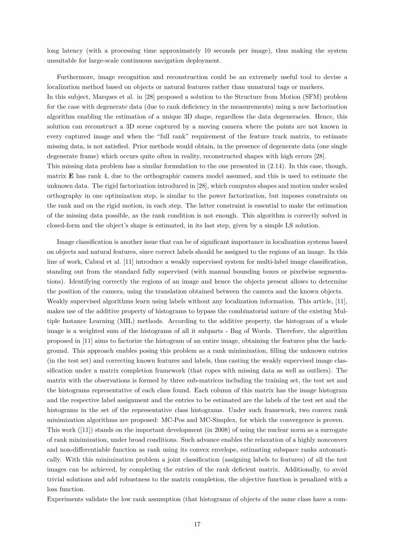
long latency (with a processing time approximately 10 seconds per image), thus making the systemunsuitable for large-scale continuous navigation deployment.

Furthermore, image recognition and reconstruction could be an extremely useful tool to devise alocalization method based on objects or natural features rather than unnatural tags or markers.In this subject, Marques et al. in [28] proposed a solution to the Structure from Motion (SFM) problemfor the case with degenerate data (due to rank deficiency in the measurements) using a new factorizationalgorithm enabling the estimation of a unique 3D shape, regardless the data degeneracies. Hence, thissolution can reconstruct a 3D scene captured by a moving camera where the points are not known inevery captured image and when the “full rank” requirement of the feature track matrix, to estimatemissing data, is not satisfied. Prior methods would obtain, in the presence of degenerate data (one singledegenerate frame) which occurs quite often in reality, reconstructed shapes with high errors [28].This missing data problem has a similar formulation to the one presented in (2.14). In this case, though,matrix E has rank 4, due to the orthographic camera model assumed, and this is used to estimate theunknown data. The rigid factorization introduced in [28], which computes shapes and motion under scaledorthography in one optimization step, is similar to the power factorization, but imposes constraints onthe rank and on the rigid motion, in each step. The latter constraint is essential to make the estimationof the missing data possible, as the rank condition is not enough. This algorithm is correctly solved inclosed-form and the object’s shape is estimated, in its last step, given by a simple LS solution.

Image classification is another issue that can be of significant importance in localization systems basedon objects and natural features, since correct labels should be assigned to the regions of an image. In thisline of work, Cabral et al. [11] introduce a weakly supervised system for multi-label image classification,standing out from the standard fully supervised (with manual bounding boxes or pixelwise segmenta-tions). Identifying correctly the regions of an image and hence the objects present allows to determinethe position of the camera, using the translation obtained between the camera and the known objects.Weakly supervised algorithms learn using labels without any localization information. This article, [11],makes use of the additive property of histograms to bypass the combinatorial nature of the existing Mul-tiple Instance Learning (MIL) methods. According to the additive property, the histogram of a wholeimage is a weighted sum of the histograms of all it subparts - Bag of Words. Therefore, the algorithmproposed in [11] aims to factorize the histogram of an entire image, obtaining the features plus the back-ground. This approach enables posing this problem as a rank minimization, filling the unknown entries(in the test set) and correcting known features and labels, thus casting the weakly supervised image clas-sification under a matrix completion framework (that copes with missing data as well as outliers). Thematrix with the observations is formed by three sub-matrices including the training set, the test set andthe histograms representative of each class found. Each column of this matrix has the image histogramand the respective label assignment and the entries to be estimated are the labels of the test set and thehistograms in the set of the representative class histograms. Under such framework, two convex rankminimization algorithms are proposed: MC-Pos and MC-Simplex, for which the convergence is proven.This work ([11]) stands on the important development (in 2008) of using the nuclear norm as a surrogateof rank minimization, under broad conditions. Such advance enables the relaxation of a highly nonconvexand non-differentiable function as rank using its convex envelope, estimating subspace ranks automati-cally. With this minimization problem a joint classification (assigning labels to features) of all the testimages can be achieved, by completing the entries of the rank deficient matrix. Additionally, to avoidtrivial solutions and add robustness to the matrix completion, the objective function is penalized with aloss function.Experiments validate the low rank assumption (that histograms of objects of the same class have a com-

17

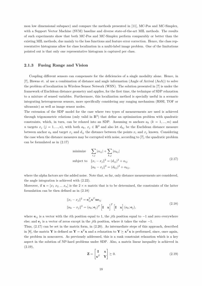
mon low dimensional subspace) and compare the methods presented in [11], MC-Pos and MC-Simplex,with a Support Vector Machine (SVM) baseline and diverse state-of-the-art MIL methods. The resultsof such experiments show that both MC-Pos and MC-Simplex perform comparably or better than theexisting MIL methods, due mainly to the loss functions and feature error correction. Hence, the class rep-resentative histograms allow for class localization in a multi-label image problem. One of the limitationspointed out is that only one representative histogram is captured per class.

2.1.3 Fusing Range and Vision

Coupling different sensors can compensate for the deficiencies of a single modality alone. Hence, in[7], Biswas et. al use a combination of distance and angle information (Angle of Arrival (AoA)) to solvethe problem of localization in Wireless Sensor Network (WSN). The solution presented in [7] is under theframework of Euclidean distance geometry and applies, for the first time, the technique of SDP relaxationto a mixture of sensed variables. Furthermore, this localization method is specially useful in a scenariointegrating heterogeneous sensors, more specifically considering any ranging mechanism (RSSI, TOF orultrasonic) as well as image sensor nodes.The extension of the SDP model for the case where two types of measurements are used is achievedthrough trigonometric relations (only valid in R2) that define an optimization problem with quadraticconstraints, which, in turn, can be relaxed into an SDP. Assuming m anchors ak (k = 1, ...,m) andn targets xj (j = 1, ..., n), with both ak, xj ∈ R2 and also let dkj be the Euclidean distance measurebetween anchor ak and target xj and dij the distance between the points xi and xj known. Consideringthe case when the distance measures may be corrupted with noise, according to [7], the quadratic problemcan be formulated as in (2.17)

minimize∑i,j

|αij |+∑k,j

|αkj |

subject to ‖xi − xj‖2 = (dij)2 + αij

‖ak − xj‖2 = (dkj)2 + αkj ,

(2.17)

where the alpha factors are the added noise. Note that, so far, only distance measurements are considered,the angle integration is achieved with (2.22).Moreover, if x = [x1 x2 ... xn] is the 2× n matrix that is to be determined, the constraints of the latterformulation can be then defined as in (2.18)

‖xi − xj‖2 = eTijxTxeij

‖ak − xj‖2 = (ak; ej)T[I x

]T [I x

](ak; ej),

(2.18)

where eij is a vector with the ith position equal to 1, the jth position equal to −1 and zero everywhereelse; and ej is a vector of zeros except in the jth position, where it takes the value −1.Thus, (2.17) can be set in the matrix form, in (2.20). As intermediate steps of this approach, describedin [8], the matrix Y is defined as Y = xTx and a relaxation to Y � xTx is performed, since, once again,the problem in nonconvex. As previously addressed, this is a rank constraint relaxation which is a keyaspect in the solution of NP-hard problems under SDP. Also, a matrix linear inequality is achieved in(2.19),

Z =[

I xxT Y

]� 0. (2.19)

18

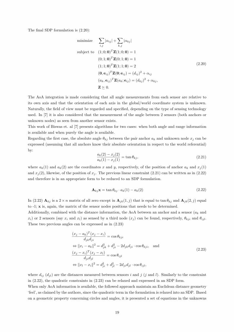
The final SDP formulation is (2.20):

minimize∑i,j

|αij |+∑k,j

|αkj |

subject to (1; 0; 0)TZ(1; 0; 0) = 1

(0; 1; 0)TZ(0; 1; 0) = 1

(1; 1; 0)TZ(1; 1; 0) = 2

(0, eij)TZ(0; eij) = (dij)2 + αij

(ak, eij)TZ(ak; eij) = (dkj)2 + αkj ,

Z � 0.

(2.20)

The AoA integration is made considering that all angle measurements from each sensor are relative toits own axis and that the orientation of each axis in the global/world coordinate system is unknown.Naturally, the field of view must be regarded and specified, depending on the type of sensing technologyused. In [7] it is also considered that the measurement of the angle between 2 sensors (both anchors orunknown nodes) as seen from another sensor exists.This work of Biswas et. al [7] presents algorithms for two cases: when both angle and range informationis available and when purely the angle is available.Regarding the first case, the absolute angle θkj between the pair anchor ak and unknown node xj can beexpressed (assuming that all anchors know their absolute orientation in respect to the world referential)by:

ak(2)− xj(2)ak(1)− xj(1) = tan θkj , (2.21)

where ak(1) and ak(2) are the coordinates x and y, respectively, of the position of anchor ak and xj(1)and xj(2), likewise, of the position of xj . The previous linear constraint (2.21) can be written as in (2.22)and therefore is in an appropriate form to be reduced to an SDP formulation.

Akjx = tan θkj · ak(1)− ak(2) (2.22)

In (2.22) Akj is a 2× n matrix of all zero except in Ajk(1, j) that is equal to tan θkj and Ajk(2, j) equalto -1; x is, again, the matrix of the sensor nodes positions that needs to be determined.Additionally, combined with the distance information, the AoA between an anchor and a sensor (ak andxi) or 2 sensors (say xi and xl) as sensed by a third node (xj) can be found, respectively, θkji and θijl.These two previous angles can be expressed as in (2.23)

(xj − ak)T (xj − xi)djkdji

= cos θkji

⇔ ‖xi − ak‖2 = d2jk + d2

ji − 2djkdji · cos θkji, and(xj − xi)T (xj − xl)

djidjl= cos θijl

⇔ ‖xl − xi‖2 = d2ji + d2

jl − 2djidjl · cos θijl,

(2.23)

where dij (djl) are the distances measured between sensors i and j (j and l). Similarly to the constraintin (2.22), the quadratic constraints in (2.23) can be relaxed and expressed in an SDP form.When only AoA information is available, the followed approach maintain an Euclidean distance geometry‘feel’, as claimed by the authors, since the quadratic term in the formulation is relaxed into an SDP. Basedon a geometric property concerning circles and angles, it is presented a set of equations in the unknowns

19

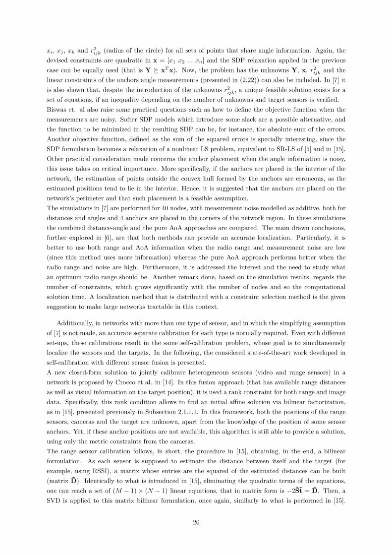
xi, xj , xk and r2ijk (radius of the circle) for all sets of points that share angle information. Again, the

devised constraints are quadratic in x = [x1 x2 ... xn] and the SDP relaxation applied in the previouscase can be equally used (that is Y � xTx). Now, the problem has the unknowns Y, x, r2

ijk and thelinear constraints of the anchors angle measurements (presented in (2.22)) can also be included. In [7] itis also shown that, despite the introduction of the unknowns r2

ijk, a unique feasible solution exists for aset of equations, if an inequality depending on the number of unknowns and target sensors is verified.Biswas et. al also raise some practical questions such as how to define the objective function when themeasurements are noisy. Softer SDP models which introduce some slack are a possible alternative, andthe function to be minimized in the resulting SDP can be, for instance, the absolute sum of the errors.Another objective function, defined as the sum of the squared errors is specially interesting, since theSDP formulation becomes a relaxation of a nonlinear LS problem, equivalent to SR-LS of [5] and in [15].Other practical consideration made concerns the anchor placement when the angle information is noisy,this issue takes on critical importance. More specifically, if the anchors are placed in the interior of thenetwork, the estimation of points outside the convex hull formed by the anchors are erroneous, as theestimated positions tend to lie in the interior. Hence, it is suggested that the anchors are placed on thenetwork’s perimeter and that such placement is a feasible assumption.The simulations in [7] are performed for 40 nodes, with measurement noise modelled as additive, both fordistances and angles and 4 anchors are placed in the corners of the network region. In these simulationsthe combined distance-angle and the pure AoA approaches are compared. The main drawn conclusions,further explored in [6], are that both methods can provide an accurate localization. Particularly, it isbetter to use both range and AoA information when the radio range and measurement noise are low(since this method uses more information) whereas the pure AoA approach performs better when theradio range and noise are high. Furthermore, it is addressed the interest and the need to study whatan optimum radio range should be. Another remark done, based on the simulation results, regards thenumber of constraints, which grows significantly with the number of nodes and so the computationalsolution time. A localization method that is distributed with a constraint selection method is the givensuggestion to make large networks tractable in this context.

Additionally, in networks with more than one type of sensor, and in which the simplifying assumptionof [7] is not made, an accurate separate calibration for each type is normally required. Even with differentset-ups, these calibrations result in the same self-calibration problem, whose goal is to simultaneouslylocalize the sensors and the targets. In the following, the considered state-of-the-art work developed inself-calibration with different sensor fusion is presented.A new closed-form solution to jointly calibrate heterogeneous sensors (video and range sensors) in anetwork is proposed by Crocco et al. in [14]. In this fusion approach (that has available range distancesas well as visual information on the target position), it is used a rank constraint for both range and imagedata. Specifically, this rank condition allows to find an initial affine solution via bilinear factorization,as in [15], presented previously in Subsection 2.1.1.1. In this framework, both the positions of the rangesensors, cameras and the target are unknown, apart from the knowledge of the position of some sensoranchors. Yet, if these anchor positions are not available, this algorithm is still able to provide a solution,using only the metric constraints from the cameras.The range sensor calibration follows, in short, the procedure in [15], obtaining, in the end, a bilinearformulation. As each sensor is supposed to estimate the distance between itself and the target (forexample, using RSSI), a matrix whose entries are the squared of the estimated distances can be built(matrix D). Identically to what is introduced in [15], eliminating the quadratic terms of the equations,one can reach a set of (M − 1) × (N − 1) linear equations, that in matrix form is −2St = D. Then, aSVD is applied to this matrix bilinear formulation, once again, similarly to what is performed in [15].

20

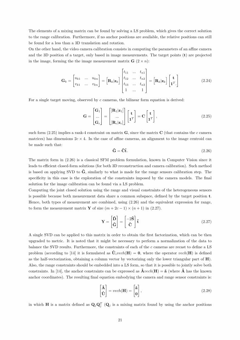
The elements of a mixing matrix can be found by solving a LS problem, which gives the correct solutionto the range calibration. Furthermore, if no anchor positions are available, the relative positions can stillbe found for a less than a 3D translation and rotation.On the other hand, the video camera calibration consists in computing the parameters of an affine cameraand the 3D position of a target, only based in image measurements. The target points (t) are projectedin the image, forming the the image measurement matrix G (2× n):

Gk =[uk1 ... ukn

vk1 ... vkn

]=[Rk|zk

]t11 ... tn1

t12 ... tn2

t13 ... tn3

1 ... 1

=[Rk|zk

] [ t1T .

](2.24)

For a single target moving, observed by c cameras, the bilinear form equation is derived:

G =

G1

...

Gc

=

[R1|z1]...

[Rc|zc]

[ t1T

]= C

[t

1T

], (2.25)

such form (2.25) implies a rank-4 constraint on matrix G, since the matrix C (that contains the c cameramatrices) has dimensions 2c × 4. In the case of affine cameras, an alignment to the image centroid canbe made such that:

G = Ct. (2.26)

The matrix form in (2.26) is a classical SFM problem formulation, known in Computer Vision since itleads to efficient closed-form solutions (for both 3D reconstruction and camera calibration). Such methodis based on applying SVD to G, similarly to what is made for the range sensors calibration step. Thespecificity in this case is the exploration of the constraints imposed by the camera models. The finalsolution for the image calibration can be found via a LS problem.Computing the joint closed solution using the range and visual constraints of the heterogeneous sensorsis possible because both measurement data share a common subspace, defined by the target position t.Hence, both types of measurement are combined, using (2.26) and the equivalent expression for range,to form the measurement matrix Y of size (m+ 2c− 1)× (n+ 1) in (2.27).

Y =[DG

]=[−2SC

]t (2.27)

A single SVD can be applied to this matrix in order to obtain the first factorization, which can be thenupgraded to metric. It is noted that it might be necessary to perform a normalization of the data tobalance the SVD results. Furthermore, the constraints of each of the c cameras are recast to define a LSproblem (according to [14] it is formulated as Uivech(H) = 0, where the operator vech(H) is definedas the half-vectorization, obtaining a column vector by vectorizing only the lower triangular part of H).Also, the range constraints should be embedded into a LS form, so that it is possible to jointly solve bothconstraints. In [14], the anchor constraints can be expressed as Avech(H) = a (where A has the knownanchor coordinates). The resulting final equation embodying the camera and range sensor constraints is:[

AU

]= vech(H) =

[a0

], (2.28)

in which H is a matrix defined as QjQTj (Qj is a mixing matrix found by using the anchor positions

21

and camera models constraints together). To compute H, equation in (2.29) can be solved simply witha pseudo-inverse:

vech(H) = (FTF)−1FT r, where F =[AU

]and r =

[a0

]. (2.29)

A real test was performed with a RGB-D device (that generates a high number of range measurementscoupled with standard images). In this test, the data matrix Y allowed to obtain the target 3D position,for each instant, together with the 3D location of the depth sensor and the camera parameters.As future work, Crocco et al., in [14], mention the extension to the missing data case in order to allowmore complex and larger networks to be also calibrated according to this method.

Discussion of existing hybrid schemesAlthough the clear relevance of the work by Biswas et al. in [7] and Crocco et al. in [14], the approachproposed in this dissertation differs from the previous and goes beyond, since it surpasses the limitationspresent in [7, 14]. More specifically, [7] shows a space dimensionality constraint, as the proposed methodcan be applied exclusively in 2D and in [14] there is a limitation of the observations, since observationsof the same target points must be performed with the different sensors (range and video). In thisdissertation work, however, two distinct sets of target points (in two different networks) in the 3D spacewill be sensed by the heterogeneous sensors: a set of wireless sensor nodes and a set of objects; thus thevector to be estimated is larger than the one in [14], as the position estimation of both types of targets,which produce different measurements, is sought. Moreover, a seamless and natural integration of bothtypes of information is pursued. Range information (either from acoustic or radio signals as Wi-Fi andfrom image properties) and pose/shape (from time varying range or pose estimation from vision) areharmoniously integrated in the same formulation. The fact that range information will depend on thetranslation between the source and the sensor while pose will depend not only on the translation butalso on the rotation matrix leads to a formulation with two minimization problems (one related to theobserved objects and the other to the estimated distances) in which the translation vector is the same.

22

Chapter 3

Methodologies

This Chapter addresses the approach followed throughout the work in order to solve the proposedproblem for this thesis, describing the new methodologies devised for such purpose. The single-sourcehybrid localization was the first issue to be tackled, thus a new method that fuses distance and angleinformation to perform a target localization is proposed in Section 3.1, including a novel optimizationbased formulation for such hybrid scenarios. Such formulation is presented in detail in Subsection 3.1.1and a procedure to solve the self-calibration problem of the different sensor networks, which emergedwhen implementing the hybrid localization algorithm in a real scenario, is described in Subsection 3.1.2.An extension of the hybrid localization to a multi-source node scenario, aiming a cooperative paradigm,is proposed in Section 3.2. The optimization criterion is similar to the one for the single-source case, butthe actual solution algorithm is entirely different and aimed at large problem sizes that often arise in thecollaborative paradigm, even for a relatively modest number of network nodes.

3.1 Single Source Hybrid Localization algorithm

3.1.1 Localization based on ranges and vision - FLORIS

In order to perform the fusion between range measurements from sensor anchor nodes and visualinformation gathered from video, a joint formulation was developed and is presented in this Section.This formulation, named FLORIS from Fusion Localization using Ranges and Incident Streaks, exhibitssome similarities to the SLCP algorithm [34] (described in Subsection 2.1.1) and is extended to 3D spaceusing a variation of the technique adopted in the SLNN algorithm, also from [34].Assuming an environment with two sensor networks comprising different types of anchors, namely, (1) sen-sor nodes that can retrieve the time of flight thus returning range information, and (2) camera-equippednodes that can retrieve visual features, it is possible to estimate the current localization of a target, basedon measurements from the hybrid network.An illustrative example of the assumed configuration/scenario is depicted in Figure 3.1, where a targetnode moves in an environment including a wireless sensor network and visual features.

23

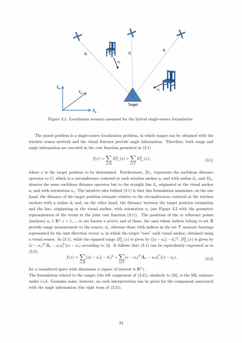
di

Xw

ZwYw

ui

ui

Target

Figure 3.1: Localizaion scenario assumed for the hybrid single-source formulation

The posed problem is a single-source localization problem, in which ranges can be obtained with thewireless sensor network and the visual features provide angle information. Therefore, both range andangle information are encoded in the cost function presented in (3.1)

f(x) =∑i∈R

D2Ci

(x) +∑i∈T

D2Li

(x), (3.1)

where x is the target position to be determined. Furthermore, DCirepresents the euclidean distance

operator to Ci which is a circumference centered at each wireless anchor ai and with radius di, and DLi

denotes the same euclidean distance operator but to the straight line Li originated at the visual anchorai and with orientation ui. The intuitive idea behind (3.1) is that this formulation minimizes, on the onehand, the distance of the target position estimate relative to the circumferences centered at the wirelessanchors with a radius di and, on the other hand, the distance between the target position estimationand the line, originating at the visual anchor, with orientation ui (see Figure 3.2 with the geometricrepresentation of the terms in the joint cost function (3.1)). The positions of the m reference points(anchors) ai ∈ Rn, i = 1, ...,m are known a priori, and of these, the ones whose indices belong to set Rprovide range measurement to the source, di, whereas those with indices in the set T measure bearingsrepresented by the unit direction vector ui in which the target “sees” each visual anchor, obtained usinga visual sensor. In (3.1), while the squared range D2

Ci(x) is given by (‖x− ai‖− di)2, D2

Li(x) is given by

(x − ai)T (In − uiuTi )(x − ai) according to [4]. It follows that (3.1) can be equivalently expressed as in(3.2),

f(x) =∑i∈R

(‖x− ai‖ − di)2 +∑i∈T

(x− ai)T (In − uiuTi )(x− ai), (3.2)

for a considered space with dimension n (space of interest is Rn).The formulation related to the ranges (the left component of (3.2)), similarly to [34], is the ML estimateunder i.i.d. Gaussian noise, however, no such interpretation can be given for the component associatedwith the angle information (the right term of (3.2)).

24

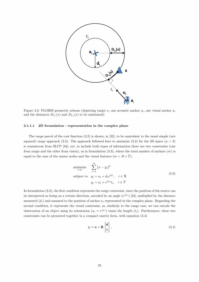
ai

di

DCi(x)

x

ai

ui

Ci

Li

Figure 3.2: FLORIS geometric scheme (depicting target x, one acoustic anchor ai, one visual anchor aiand the distances DCi(x) and DLi(x) to be minimized)

3.1.1.1 2D formulation - representation in the complex plane

The range parcel of the cost function (3.2) is shown, in [32], to be equivalent to the usual simple (notsquared) range approach (2.2). The approach followed here to minimize (3.2) for the 2D space (n = 2)is reminiscent from SLCP [34], yet, to include both types of information there are two constraints (onefrom range and the other from vision), as in formulation (3.3), where the total number of anchors (m) isequal to the sum of the sensor nodes and the visual features (m = R+ T ).

minimizex,yi

m∑i=1‖x− yi‖2

subject to yi = ai + diejφi , i ∈ R

yi = ai + ejϕiti, i ∈ T

(3.3)

In formulation (3.3), the first condition represents the range constraint, since the position of the source canbe interpreted as being on a certain direction, encoded by an angle (ejφi) [34], multiplied by the distancemeasured (di) and summed to the position of anchor ai represented in the complex plane. Regarding thesecond condition, it represents the visual constraint, as, similarly to the range case, we can encode theobservation of an object using its orientation (ui = ejϕi) times the length (ti). Furthermore, these twoconstraints can be presented together in a compact matrix form, with equation (3.4)

y = a + R[

θ

t

], (3.4)

25

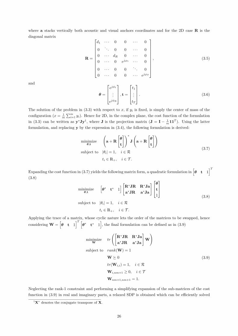
where a stacks vertically both acoustic and visual anchors coordinates and for the 2D case R is thediagonal matrix

R =

d1 · · · 0 0 · · · 0

0. . . 0 0 · · · 0

0 · · · dR 0 · · · 00 · · · 0 ejϕ1 · · · 0

0 · · · 0 0. . . 0

0 · · · 0 0 · · · ejϕT

, (3.5)

and

θ =

ejφ1

...ejφR

, t =

t1...tT

. (3.6)

The solution of the problem in (3.3) with respect to x, if yi is fixed, is simply the center of mass of theconfiguration (x = 1

m

∑mi=1 yi). Hence for 2D, in the complex plane, the cost function of the formulation

in (3.3) can be written as y∗Jy1, where J is the projection matrix (J = I − 1m11T ). Using the latter

formulation, and replacing y by the expression in (3.4), the following formulation is derived:

minimizeθ,t

(a + R

[θ

t

])∗J(

a + R[

θ

t

])subject to |θi| = 1, i ∈ R

ti ∈ R+, i ∈ T .

(3.7)

Expanding the cost function in (3.7) yields the following matrix form, a quadratic formulation in[θ t 1

]T(3.8)

minimizeθ,t

[θ∗ t∗ 1

] [R∗JR R∗Jaa∗JR a∗Ja

]θ

t1

subject to |θi| = 1, i ∈ R

ti ∈ R+, i ∈ T .

(3.8)

Applying the trace of a matrix, whose cyclic nature lets the order of the matrices to be swapped, henceconsidering W =

[θ t 1

]T [θ∗ t∗ 1

], the final formulation can be defined as in (3.9)

minimizeW

tr

([R∗JR R∗Jaa∗JR a∗Ja

]W)

subject to rank(W) = 1

W � 0

tr(Wi,i) = 1, i ∈ R

Wi,nm+1 ≥ 0, i ∈ T

Wnm+1,nm+1 = 1.

(3.9)

Neglecting the rank-1 constraint and performing a simplifying expansion of the sub-matrices of the costfunction in (3.9) in real and imaginary parts, a relaxed SDP is obtained which can be efficiently solved

1X∗ denotes the conjugate transpose of X.

26

using generic solvers. In this way, the goals of finding the phases vector θ as well as the translationsvector t are jointly achieved, through matrix W, provided that its rank is (at least approximately) one.Finally, the source position x is estimated as the average of the m points of yi, defined according to (3.4),which are directly obtained from the rightmost column (or bottom row) of W.Alternatively, it is possible to obtain, in a first step, only the phase vector θ, from the matrix W in theSDP problem (3.9) and, afterwards, use this vector to minimize the cost function relative to t.It was verified that the resulting estimated source positions are similar for both approaches.

3.1.1.2 3D formulation

To solve this problem in 3D, only minor changes are applied. More specifically, considering the 3Dspace, the variables are no longer represented using the complex plane, therefore the formulation for R3

is in (3.10).

minimizex,yi∈R3

m∑i=1‖x− yi‖2

subject to yi = ai + diθi, ‖θi‖ = 1, i ∈ R

yi = ai + uiti, ti ∈ R+, i ∈ T

(3.10)

Comparing the latter formulation in (3.10) with (3.3), it is possible to notice that the performed 2Dgeometric interpretation is now extended to the 3D case, in which θi plays the same role as ejφi and ui

takes the place of ejϕi . Similarly to the 2D case, the cost function in (3.10) can be expressed as yTJy,which allows to follow the same rationale.Furthermore, matrix R as well as the projection matrix J are now defined as follows:

R =

d1 0 0 0 0 0 · · · 0 0 0 0 0 · · · 00 d1 0 0 0 0 · · · 0 0 0 0 0 · · · 00 0 d1 0 0 0 · · · 0 0 0 0 0 · · · 00 0 0 d2 0 0 · · · 0 0 0 0 0 · · · 00 0 0 0 d2 0 · · · 0 0 0 0 0 · · · 00 0 0 0 0 d2 · · · 0 0 0 0 0 · · · 0

0 0 0 0 0 0. . . 0 0 0 0 0 · · · 0

0 0 0 0 0 0 · · · dR 0 0 0 0 · · · 00 0 0 0 0 0 · · · 0 dR 0 0 0 · · · 00 0 0 0 0 0 · · · 0 0 dR 0 0 · · · 00 0 0 0 0 0 · · · 0 0 0 u1x 0 · · · 00 0 0 0 0 0 · · · 0 0 0 u1y 0 · · · 00 0 0 0 0 0 · · · 0 0 0 u1z 0 · · · 00 0 0 0 0 0 · · · 0 0 0 0 u2x · · · 00 0 0 0 0 0 · · · 0 0 0 0 u2y · · · 00 0 0 0 0 0 · · · 0 0 0 0 u2z · · · 0

0 0 0 0 0 0 · · · 0 0 0 0 0. . . 0

0 0 0 0 0 0 · · · 0 0 0 0 0 · · · uTx

0 0 0 0 0 0 · · · 0 0 0 0 0 · · · uTy

0 0 0 0 0 0 · · · 0 0 0 0 0 · · · uTz

, (3.11)

27

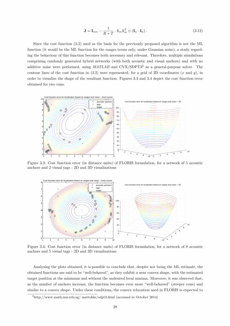
J = Imn −1

R+ T· 1m1Tm ⊗ (In · In) . (3.12)

Since the cost function (3.2) used as the basis for the previously proposed algorithm is not the MLfunction (it would be the ML function for the ranges terms only, under Gaussian noise), a study regard-ing the behaviour of this function becomes both necessary and relevant. Therefore, multiple simulationscomprising randomly generated hybrid networks (with both acoustic and visual anchors) and with noadditive noise were performed, using MATLAB and CVX/SDPT32 as a general-purpose solver. Thecontour lines of the cost function in (3.2) were represented, for a grid of 2D coordinates (x and y), inorder to visualize the shape of the resultant function. Figures 3.3 and 3.4 depict the cost function errorobtained for two runs.

0 1 2 3 4 5 6 7 8 90

1

2

3

4

5

6

7

8

9

10Cost function error for localization based on ranges and vision − level curves

5

10

15

15

20

20

25

25

30

30

35

35

40

40

45

45

50

50

55

55

60 60

60

65

65

65

70

70

70

7575

75

80

80

8085

85

85

90

90

90

95

95

95

100

100

100

acoustic anchorstagstarget

0 24 6 8 10 0 2 4 6 8 10

0

10

20

30

40

50

60

70

80

90

100

Cost function error for localization based on ranges and vision − 3D

Figure 3.3: Cost function error (in distance units) of FLORIS formulation, for a network of 5 acousticanchors and 2 visual tags - 2D and 3D visualizations

1 2 3 4 5 6 7 8 9 100

1

2

3

4

5

6

7

8Cost function error for localization based on ranges and vision − level curves

5

1015 20

2025

25

30

30

35

35

40

40

45

45

50

50

55

55

60

60

65

65

70

70

75

75

7580

80

80

85

85

85

90

90

90

95

95

95

100

100

100

acoustic anchorstagstarget

02

46

810 0

2

4

6

8

10

0

20

40

60

80

100

Cost function error for localization based on ranges and vision − 3D

Figure 3.4: Cost function error (in distance units) of FLORIS formulation, for a network of 8 acousticanchors and 5 visual tags - 2D and 3D visualizations

Analysing the plots obtained, it is possible to conclude that, despite not being the ML estimate, theobtained functions are said to be “well-behaved”, as they exhibit a near convex shape, with the estimatedtarget position at the minimum and without the undesired local minima. Moreover, it was observed that,as the number of anchors increase, the function becomes even more “well-behaved” (steeper cone) andsimilar to a convex shape. Under these conditions, the convex relaxation used in FLORIS is expected to

2http://www.math.nus.edu.sg/ mattohkc/sdpt3.html (accessed in October 2014)

28

yield an (approximately) rank-1 solution with high probability.A thorough set of simulations were performed on randomly generated networks in order to characterizeand test the performance of the previously proposed algorithm. Chapter 4 presents the results of suchsimulations. A performance comparison with other two state-of-the-art single-source methods indicatesa leading performance of FLORIS for high noise cases, due to the particular robustness of the estimatesaccuracy in such scenarios.The first experimental set-up developed to implement this hybrid localization algorithm consisted of avideo camera mounted in a solidary way with a Cricket listener node. The most relevant tests performedand results obtained in this set-up are, also, presented and discussed in Chapter 4. In this case, thepractical feasibility of FLORIS is completely attested, as the results attained surpass in accuracy theones provided by the other methods, for the same experimental dataset.

It should be highlighted that the above proposed hybrid localization algorithm differs from the meth-ods presented in Chapter 2, particularly, [7] and [14], thus making a novel contribution to this field. In theproposed scenario for this thesis there are two separate networks of heterogeneous sensors which detectand measure different variables, namely range and angle from vision. However, in the work found inthe state-of-the-art, only one network of sensors that are able to simultaneously measure different typesof variables is explored. Additionally, FLORIS, adopts the same strategy for relaxation used in SLCPin [34], and thus provides a very tight approximation to the original nonconvex problem, conferring abetter performance when compared to the R-LS method in [5]. Besides the aforementioned aspects, insuch previous works only simulation results are presented yielding neither deployment nor experimentaltests in a real scenario.

3.1.2 Self-calibration process for the two separate sensor networks

From the existence of the two detached sensor networks, which contrasts with the related work found(more specifically in [7, 14]), emerged the need to calibrate both networks, as a precondition to performlocalization. In fact, in [7] it is assumed that the obtained measurements are the absolute angles, sinceall the anchor nodes are aware of their orientation relative to the global coordinate system. This differsfrom our scenario, in which the network of sensors measuring angles is detached from the network ofranging sensors. Hence, such assumption cannot be made and a method to relate and determine thetransformation between the two is required. The present Subsection details the process developed toachieve such calibration. We highlight that this is another major original contribution of this dissertation.To fuse the information conveyed by both sensors, which belong to two different sensor networks, bothmeasurements have to be referenced in a common coordinate system. However, as shown in Figure 3.5,the acoustic anchors form a network detached from the network of the visual features. As each networkhas its own separate coordinate system (coordinate system denoted as c for the sensor network and a

for the visual anchors), it becomes necessary to define a global referential. Furthermore, Figure 3.5depicts the target (a device comprising a video camera that can measure transformations to the visualmarkers attached to an acoustic sensor that can gather range measurements to the wireless sensor nodes)performing a trajectory in the localization scenario which includes both types of anchor nodes and allthe translations and rotations that can be measured or should be determined through the calibrationprocess.In this case, the range measurements obtained acoustically will lead to a target position estimation in

29

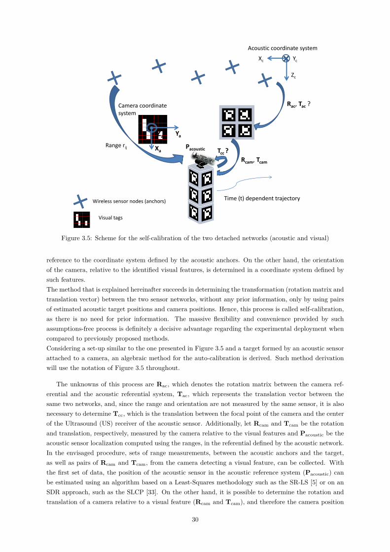
Rcam

, Tcam

Range rij

Rac

, Tac

?

Acoustic coordinate system

Wireless sensor nodes (anchors)

Visual tags

Camera coordinate

system

Xc

Zc

Yc

Tcc

?

Ya

Xa

Za

Pacoustic

Time (t) dependent trajectory

Figure 3.5: Scheme for the self-calibration of the two detached networks (acoustic and visual)

reference to the coordinate system defined by the acoustic anchors. On the other hand, the orientationof the camera, relative to the identified visual features, is determined in a coordinate system defined bysuch features.The method that is explained hereinafter succeeds in determining the transformation (rotation matrix andtranslation vector) between the two sensor networks, without any prior information, only by using pairsof estimated acoustic target positions and camera positions. Hence, this process is called self-calibration,as there is no need for prior information. The massive flexibility and convenience provided by suchassumptions-free process is definitely a decisive advantage regarding the experimental deployment whencompared to previously proposed methods.Considering a set-up similar to the one presented in Figure 3.5 and a target formed by an acoustic sensorattached to a camera, an algebraic method for the auto-calibration is derived. Such method derivationwill use the notation of Figure 3.5 throughout.

The unknowns of this process are Rac, which denotes the rotation matrix between the camera ref-erential and the acoustic referential system, Tac, which represents the translation vector between thesame two networks, and, since the range and orientation are not measured by the same sensor, it is alsonecessary to determine Tcc, which is the translation between the focal point of the camera and the centerof the Ultrasound (US) receiver of the acoustic sensor. Additionally, let Rcam and Tcam be the rotationand translation, respectively, measured by the camera relative to the visual features and Pacoustic be theacoustic sensor localization computed using the ranges, in the referential defined by the acoustic network.In the envisaged procedure, sets of range measurements, between the acoustic anchors and the target,as well as pairs of Rcam and Tcam, from the camera detecting a visual feature, can be collected. Withthe first set of data, the position of the acoustic sensor in the acoustic reference system (Pacoustic) canbe estimated using an algorithm based on a Least-Squares methodology such as the SR-LS [5] or on anSDR approach, such as the SLCP [33]. On the other hand, it is possible to determine the rotation andtranslation of a camera relative to a visual feature (Rcam and Tcam), and therefore the camera position

30

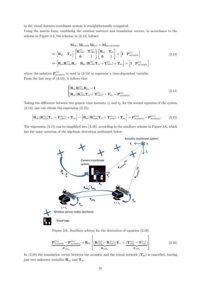
in the visual features coordinate system is straightforwardly computed.Using the matrix form, combining the rotation matrices and translation vectors, in accordance to thescheme in Figure 3.5, the relation in (3.13) follows

MAC MCAM MCC = MACOUSTIC

⇔[Rac Tac

] [R(t)cam T(t)

cam

0 1

][Rcc Tcc

0 1

]=[I P(t)

acoustic

]⇔[RacR(t)

camRcc Rac(R(t)camTcc + T(t)

cam) + Tac

]=[I P(t)

acoustic

],

(3.13)

where the notation P(t)acoustic is used in (3.13) to represent a time-dependent variable.

From the last step of (3.13), it follows thatRacR(t)camRcc = I

Rac(R(t)camTcc + T(t)

cam) + Tac = P(t)acoustic.

(3.14)

Taking the difference between two generic time instants, t1 and t2, for the second equation of the system(3.14), one can obtain the expression (3.15):[

Rac(R(t2)camTcc + T(t2)

cam) + Tac

]−[Rac(R(t1)

camTcc + T(t1)cam) + Tac

]= P(t2)

acoustic −P(t1)acoustic. (3.15)

The expression (3.15) can be simplified into (3.16), according to the auxiliary scheme in Figure 3.6, whichhas the same notation of the algebraic derivation performed below.

Wireless sensor nodes (anchors)

Visual tags

Acoustic coordinate system

Xc

Zc

Yc

Camera coordinate

system

Xa

ZaYa

t = t1

t = t2Tcc

Tcc

Rdiffk, Tdiffk

Pdiffk

Figure 3.6: Auxiliary scheme for the derivation of equation (3.16)

P(t2)acoustic −P(t1)

acoustic︸ ︷︷ ︸Pdiffk

= Rac

(R(t2)cam −R(t1)

cam)︸ ︷︷ ︸Rdiffk

Tcc + (T(t2)cam −T(t1)

cam)︸ ︷︷ ︸Tdiffk

(3.16)

In (3.16) the translation vector between the acoustic and the visual network (Tac) is cancelled, leavingjust two unknown variables Rac and Tcc.

31

Appending/stacking horizontally all the N (number of measurements −1) pairwise differences measured,equation (3.16) can be expressed as in (3.17)

[Pdiff1 · · ·PdiffN]︸ ︷︷ ︸Pdiff

= Rac

[Rdiff1Tcc · · ·RdiffNTcc]︸ ︷︷ ︸Rdiff(IN ⊗Tcc)

+ [Tdiff1 · · ·TdiffN ]︸ ︷︷ ︸Tdiff

, (3.17)

where IN denotes an identity matrix of N × N , Rdiff is formed by horizontally stacked differences ofrotations matrices (which no longer hold the properties of a rotation matrix) and Tdiff includes thepairwise differences of translation vectors.According to (3.17), the error function can be defined as

E = [Pdiff −Rac (Rdiff(IN ⊗Tcc) + Tdiff)] . (3.18)

With this formulation, Rac can be estimated by solving an orthogonal Procrustes problem3, which deter-mines the closest orthogonal rotation matrix that best fits two sets of points. Here, one set of points isgiven by Pdiff (which are the pairwise differences of the position estimations obtained through the acous-tic sensor network, alone) and the other by Rdiff(IN ⊗Tcc) + Tdiff, hence the solution of the Procrustesproblem will give an estimate of Rac.In order to reduce the complexity of the algebraic calculations in such cases, the Frobenius norm is usu-ally applied. Since one of the ways in which this norm can be defined is ‖A‖2F = tr(A∗A) , we applythe trace operator to E∗E, thus tr{E∗E}. Taking the trace truly simplifies the calculations, since theexpression is transformed in an inner-product (element-wise computation), while no information is lost,as the eigenvalues hold all the matrix information. This can also be regarded as computing the averageof the error covariance matrix.After some algebraic manipulation, a new expression for the error function is obtained in (3.19)4.

E(Tcc,Rac) = tr{PTdiffPdiff − 2PT

diffRac (RdiffIN ⊗Tcc + Tcam) + (IN ⊗Tcc)TRTdiffRdiff(IN ⊗Tcc)+

2TTcamRdiffIN ⊗Tcc + TT

camTcam}(3.19)

To determine the unknown Tcc, we should minimize the error, thereby, using the function E(Tcc,Rac),defined in (3.19) to form the cost function, yields the following optimization problem in (3.20).

minimizeRac,Tcc

tr{PTdiffPdiff − 2PT

diffRac (RdiffIN ⊗Tcc + Tcam) + (IN ⊗Tcc)TRTdiffRdiff(IN ⊗Tcc)

+ 2TTcamRdiffIN ⊗Tcc + TT

camTcam}

subject to RTacRac = I3

(3.20)The problem in (3.20) is a constrained optimization problem, since the matrix Rac has to belong to thespace of rotation matrices. Consequently, the method to minimize this objective function consists in usingthe Lagrange multipliers so that this problem is converted into an unconstrained optimization problem(the restriction is incorporated in the same equation as the cost function). The auxiliary function givenby the Lagrangian method is shown in (3.21)

L(Tcc,Rac, λ) = E(Tcc,Rac) + tr(λ(RTacRac − I3)), (3.21)

3http://en.wikipedia.org/wiki/Orthogonal Procrustes problem (accessed in October 2014)4As all the values are real (positions in the 3D space and rotation matrices), the conjugate transpose notation

(X∗) is replaced, simply, by the transpose (XT ).

32

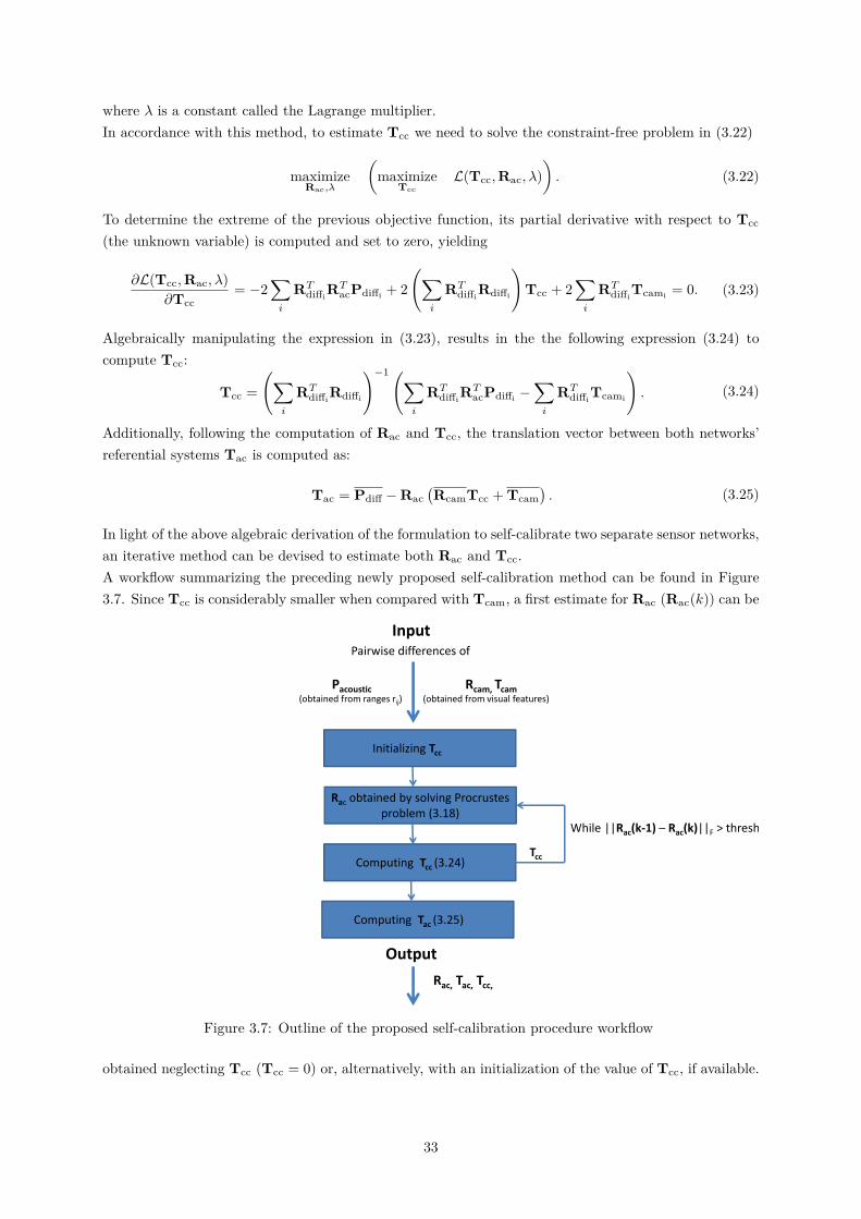
where λ is a constant called the Lagrange multiplier.In accordance with this method, to estimate Tcc we need to solve the constraint-free problem in (3.22)

maximizeRac,λ

(maximize

TccL(Tcc,Rac, λ)

). (3.22)

To determine the extreme of the previous objective function, its partial derivative with respect to Tcc

(the unknown variable) is computed and set to zero, yielding

∂L(Tcc,Rac, λ)∂Tcc

= −2∑i

RTdiffi

RTacPdiffi + 2

(∑i

RTdiffi

Rdiffi

)Tcc + 2

∑i

RTdiffi

Tcami = 0. (3.23)

Algebraically manipulating the expression in (3.23), results in the the following expression (3.24) tocompute Tcc:

Tcc =(∑

i

RTdiffi

Rdiffi

)−1(∑i

RTdiffi

RTacPdiffi −

∑i

RTdiffi

Tcami

). (3.24)

Additionally, following the computation of Rac and Tcc, the translation vector between both networks’referential systems Tac is computed as:

Tac = Pdiff −Rac(RcamTcc + Tcam

). (3.25)

In light of the above algebraic derivation of the formulation to self-calibrate two separate sensor networks,an iterative method can be devised to estimate both Rac and Tcc.A workflow summarizing the preceding newly proposed self-calibration method can be found in Figure3.7. Since Tcc is considerably smaller when compared with Tcam, a first estimate for Rac (Rac(k)) can be

Initializing Tcc

Input

Pairwise differences of

Pacoustic(obtained from ranges rij)

Rcam, Tcam(obtained from visual features)

Rac obtained by solving Procrustes

problem (3.18)

Computing Tcc (3.24)

Computing Tac (3.25)

Output

Rac, Tac, Tcc,

Tcc

While ||Rac(k-1) – Rac(k)||F > thresh

Figure 3.7: Outline of the proposed self-calibration procedure workflow

obtained neglecting Tcc (Tcc = 0) or, alternatively, with an initialization of the value of Tcc, if available.

33

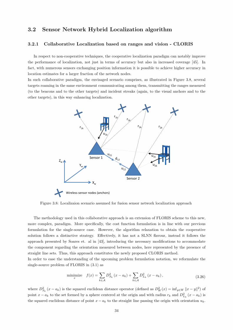
3.2 Sensor Network Hybrid Localization algorithm

3.2.1 Collaborative Localization based on ranges and vision - CLORIS

In respect to non-cooperative techniques, the cooperative localization paradigm can notably improvethe performance of localization, not just in terms of accuracy but also in increased coverage [45]. Infact, with numerous sensors exchanging position information it is possible to achieve higher accuracy inlocation estimates for a larger fraction of the network nodes.In such collaborative paradigm, the envisaged scenario comprises, as illustrated in Figure 3.8, severaltargets roaming in the same environment communicating among them, transmitting the ranges measured(to the beacons and to the other targets) and incident streaks (again, to the visual anchors and to theother targets), in this way enhancing localization.

r1k

d12

Xw

Zw

Yw

u1k

u1k

Sensor 1

r1k

Sensor 2

r2k

r1k

u12

r2k

u2k

u21

Wireless sensor nodes (anchors)

Figure 3.8: Localizaion scenario assumed for fusion sensor network localization approach

The methodology used in this collaborative approach is an extension of FLORIS scheme to this new,more complex, paradigm. More specifically, the cost function formulation is in line with our previousformulation for the single-source case. However, the algorithm relaxation to obtain the cooperativesolution follows a distinctive strategy. Effectively, it has not a SLNN flavour, instead it follows theapproach presented by Soares et. al in [43], introducing the necessary modifications to accommodatethe component regarding the orientation measured between nodes, here represented by the presence ofstraight line sets. Thus, this approach constitutes the newly proposed CLORIS method.In order to ease the understanding of the upcoming problem formulation notation, we reformulate thesingle-source problem of FLORIS in (3.1) as

minimizex

f(x) =∑k∈A

D2Sk

(x− ak) +∑k∈A

D2Lk

(x− ak) , (3.26)

where D2Sk

(x− ak) is the squared euclidean distance operator (defined as D2W (x) = infy∈W ‖x− y‖2) of

point x− ak to the set formed by a sphere centered at the origin and with radius rk and D2Lk

(x− ak) isthe squared euclidean distance of point x− ak to the straight line passing the origin with orientation uk.

34

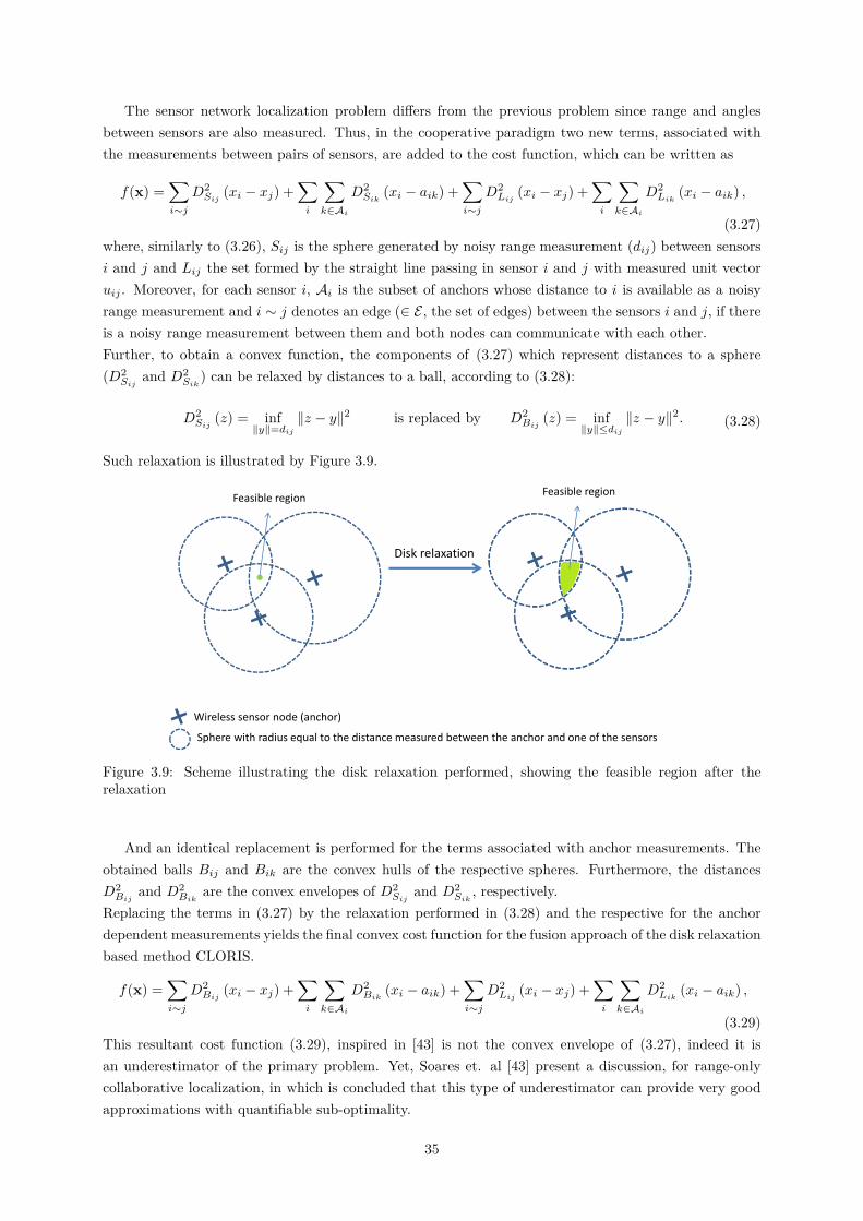
The sensor network localization problem differs from the previous problem since range and anglesbetween sensors are also measured. Thus, in the cooperative paradigm two new terms, associated withthe measurements between pairs of sensors, are added to the cost function, which can be written as

f(x) =∑i∼j

D2Sij

(xi − xj) +∑i

∑k∈Ai

D2Sik

(xi − aik) +∑i∼j

D2Lij

(xi − xj) +∑i

∑k∈Ai

D2Lik

(xi − aik) ,

(3.27)where, similarly to (3.26), Sij is the sphere generated by noisy range measurement (dij) between sensorsi and j and Lij the set formed by the straight line passing in sensor i and j with measured unit vectoruij . Moreover, for each sensor i, Ai is the subset of anchors whose distance to i is available as a noisyrange measurement and i ∼ j denotes an edge (∈ E , the set of edges) between the sensors i and j, if thereis a noisy range measurement between them and both nodes can communicate with each other.Further, to obtain a convex function, the components of (3.27) which represent distances to a sphere(D2

Sijand D2

Sik) can be relaxed by distances to a ball, according to (3.28):

D2Sij

(z) = inf‖y‖=dij

‖z − y‖2 is replaced by D2Bij

(z) = inf‖y‖≤dij

‖z − y‖2. (3.28)

Such relaxation is illustrated by Figure 3.9.

Feasible regionFeasible region

Disk relaxation

Wireless sensor node (anchor)

Sphere with radius equal to the distance measured between the anchor and one of the sensors

Figure 3.9: Scheme illustrating the disk relaxation performed, showing the feasible region after therelaxation

And an identical replacement is performed for the terms associated with anchor measurements. Theobtained balls Bij and Bik are the convex hulls of the respective spheres. Furthermore, the distancesD2Bij

and D2Bik

are the convex envelopes of D2Sij

and D2Sik

, respectively.Replacing the terms in (3.27) by the relaxation performed in (3.28) and the respective for the anchordependent measurements yields the final convex cost function for the fusion approach of the disk relaxationbased method CLORIS.

f(x) =∑i∼j

D2Bij

(xi − xj) +∑i

∑k∈Ai

D2Bik

(xi − aik) +∑i∼j

D2Lij

(xi − xj) +∑i

∑k∈Ai

D2Lik

(xi − aik) ,

(3.29)This resultant cost function (3.29), inspired in [43] is not the convex envelope of (3.27), indeed it isan underestimator of the primary problem. Yet, Soares et. al [43] present a discussion, for range-onlycollaborative localization, in which is concluded that this type of underestimator can provide very goodapproximations with quantifiable sub-optimality.

35

At this point it is important to make the following remark regarding a comparison between the relax-ation strategy followed in CLORIS and the EDM approaches discussed in the state-of-the-art. Althoughcooperative only range EDM based methods can dispense, up to a certain point, the a priori knowledgeof anchors positions, that is not the case for the present disk relaxation. Indeed, the knowledge of theanchor coordinates is crucial for this approach. Nevertheless, and as a positive feature of this disk re-laxation, while in the SDP relaxations carried out in EDM based methods a factorization, without anyrank guarantees, has to be necessarily performed, the present approach circumvents such inconvenientcomplexity. Thus, while in the EDM case we have to optimistically expect, with no guarantees, a rank-1solution, in the CLORIS case we work directly with the anchors coordinates, as discussed bellow.Now that a suitable cost function was found, the method addressed in this dissertation to obtain thesolution follows the distributed sensor network localization algorithm via the accelerated Nesterov’s gra-dient descent, introduced in [30].Following [43] and adding the terms related to the angle information, the cost function (3.29) is expressedas

minimizex

f(x) =∑i∼j

D2Bij

(Adx) +∑i∼j

D2Lij

(Alx)︸ ︷︷ ︸g(x)

+∑i

∑k∈Ai

D2Bik

(xi − aik) +∑i

∑k∈Ai

D2Lik

(xi − aik)︸ ︷︷ ︸h(x)

,

(3.30)in which matrices Ad and Al perform the coordinate differences for the acoustic and the visual anchors,respectively. These matrices are computed as Ad = Cd⊗Ip and Al = Cl⊗Ip (p is the space dimension andthis method is valid for both practical cases of p = 2 and p = 3), where Cd is the arc-node incidence matrixwith the distances of the network and Cl is the arc-node incidence matrix relative to the orientationsmeasured. The division into the sum of two functions g(x) and h(x) is useful for computing the gradientof the cost function.The function D2

Bij(z) is convex and differentiable, with gradient

∇D2Bij

(z) = z − PBij(z) , (3.31)

where PBij(z) denotes de orthogonal projection of point z onto the convex set (ball) Bij . Likewise, the

gradient of D2Lij

(z) is∇D2

Lij(z) = z − PlLij

(z) , (3.32)

PlLij(z) is the orthogonal projection of point z onto the set formed by the straight line Lij .

Hence, by (3.31), (3.32) and applying the gradient operator rules, the gradient of g(x) is obtained as in(3.33).

∇g (x) = ∇D2B (z) +∇D2

L (z)

= ATd∇D2

B (Adx) + ATl ∇D2

L (Alx)

= ATd (Adx− PB(Adx)) + AT

l (Alx− PlL(Alx))

= Ldx−ATd PB(Adx) + Llx−AT

l PlL(Alx)

(3.33)

In expression (3.33) B and L denote the Cartesian product of the balls Bij and the straight lines Lij ,corresponding to the edges with range or bearing information, respectively. Furthermore, Ld(l) is definedas Ld(l) ⊗ Ip, being Ld(l) the Laplacian matrix related to the distance (angles) graph.

36

Regarding h(x), let ∇h(x) = (∇h1(x1), ...,∇hn(xn)), where each term is:

∇hi (xi) =∑k∈Ai

∇D2Bik

(xi − aik) +∇D2Lik (xi − aik)

=∑k∈Ai

(xi − aik)− PB(xi − aik) +∑k∈Ai

(xi − aik)− PlL(xi − aik).(3.34)

From (3.33) and (3.34), the overall gradient of cost function f(x) can be computed according to expression(3.35).

∇f (x) = Ldx−ATd PB(Adx) + Llx−AT

l PlL(Alx)

+

∑k∈A1

(x1 − a1k)− PB(x1 − a1k) +∑k∈A1

(x1 − a1k)− PlL(x1 − a1k)

...∑k∈An

(xn − ank)− PB(xn − ank) +∑k∈An

(xn − ank)− PlL(xn − ank)

(3.35)

As both ∇g(x) and ∇h(x) are Lipschitz continuous functions, it is possible to compute the Lipschitzconstants, which according to [43]5 are Lg = 2δmax (δmax is the maximum sensor node degree) andLh = max |Ai| : i ∈ V (which denotes the maximum degree of the anchors nodes); for this fusion casethe graph includes both range and orientation anchors of the network. Such constants, resulting in theLipschitz constant Lf = 2δmax + max |Ai| : i ∈ V, together with the gradient of f enables the use of theparallel algorithm to minimize this cost function described below. Parallelizability is a crucial concern inthe development of distributed inference algorithms for sensor networks, but is beyond the scope of thiswork. Therefore, no advantage is taken here of the specific form of (3.35).To find the minimum of f the followed approach is the Nesterov’s optimal method [30], as in [43], sincethe cost function has a Lipschitz continuous gradient in (3.35). The choice of Nesterov’s over conventionaldescent gradient methods allows for a tremendous speed increase at almost no additional computationalcomplexity cost. At a high level, in this approach each node estimate is given an arbitrary initial valueand its position estimate (xi(k)) is updated resorting to a combination (wi) of the two previous iterationsestimates (xi(k − 1) and xi(k − 2)). The previous loop can be performed up to a predefined maximumnumber of iterations or it can stop when the gradient is smaller than a preset threshold. The pseudo-codeof this algorithm is presented in detail in Algorithm 1.

5The expressions for the Lipschitz constants in [43] were originally derived under the assumption that all setswere balls, but they still hold true even when some of these sets become lines.

37

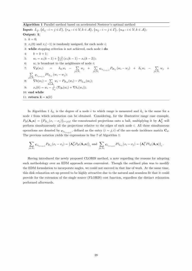
Algorithm 1 Parallel method based on accelerated Nesterov’s optimal methodInput: Lf , {dij : i ∼ j ∈ E}, {rik : i ∈ V, k ∈ A}, {uij : i ∼ j ∈ E}, {uik : i ∈ V, k ∈ A};Output: x;1: k = 0;2: xi(0) and xi(−1) is randomly assigned, for each node i;3: while stopping criterion is not achieved, each node i do4: k = k + 1;5: wi = xi(k − 1) + k−2

k+1 (xi(k − 1)− xi(k − 2));6: wi is broadcast to the neighbours of node i;7: ∇g(wi) = δdiwi −

∑j∈Ni

wj +∑j∈Ni

Cd(i∼j,i)PBij

(wi − wj) + δliwi −∑j∈Ni

wj +∑j∈Ni

Cl(i∼j,i)PlLij

(wi − wj);

8: ∇h(wi) =∑k∈Ai

wi − PBik(wi)− PlLik

(wi);

9: xi(k) = wi − 1Lf

(∇gi(wi) +∇hi(wi));10: end while11: return x = x(k)

In Algorithm 1 δdi is the degree of a node i to which range is measured and δli is the same for anode i from which orientation can be obtained. Considering, for the illustrative range case example,PB(Adx) = {PBij (xi − xj)}i∼j∈E the concatenated projections onto a ball, multiplying it by AT

d willperform simultaneously all the projections relative to the edges of each node i. All these simultaneousoperations are denoted by Cd(i∼j,i)

, defined as the entry (i ∼ j, i) of the arc-node incidence matrix Cd.The previous notation yields the expressions in line 7 of Algorithm 1:∑

j∈Ni

Cd(i∼j,i)PBij (xi − xj) =

(ATd PB(Adx)

)i

and∑j∈Ni

Cl(i∼j,i)PlLij (xi − xj) =

(ATl PlL(Alx)

)i.

Having introduced the newly proposed CLORIS method, a note regarding the reasons for adoptingsuch methodology over an EDM approach seems convenient. Though the outlined plan was to modifythe EDM formulation to incorporate angles, we could not succeed in that line of work. At the same time,this disk relaxation set-up proved to be highly attractive due to the natural and seamless fit that it couldprovide for the extension of the single source (FLORIS) cost function, regardless the distinct relaxationperformed afterwards.

38

Chapter 4

Results

In this Chapter the main simulation and experimental results attained for both FLORIS and CLORISare presented, in Sections 4.1 and 4.2, respectively.Extensive tests were run, in simulation, in order to analyse the performance of the hybrid localizationmethods proposed in this dissertation. All the conditions in which such tests were run, as well as theoutcomes, are detailed in Subsections 4.1.1 and 4.2.1.As an experimental testbed for indoor localization was also developed in the scope of this thesis, findingsfrom applying the new hybrid algorithms on a real scenario are addressed in Subsections 4.1.2 and 4.2.2.Moreover, is included a quantitative performance analysis, benchmarking FLORIS and CLORIS againstmethods found in the literature, aiming to demonstrate the improvements introduced by the contributionsgiven in this work.Regarding the experimental implementation, some hardware details as well as physical limitations (someovercome, while others not) are also discussed.

4.1 Single Source Localization - FLORIS

4.1.1 Simulation

4.1.1.1 Preliminaries

In order to assess the performance of the hybrid localization algorithm proposed in this thesis, severalsimulation tests were performed. Both the position estimation error and the rank of matrix W werestudied. The analysis of the rank of W allows to assess the formulation in (3.9) and its relaxation, sincewhen rank(W) = 1, the relaxed solution coincides with the optimal one for the non-relaxed and originalproblem.The following experiments were run using MATLAB R2013a and the general-purpose SDP solver CVX/S-DPT31. Networks of acoustic and visual anchors were randomly generated in a [0, 5] × [0, 5] × [0, 5] cubewith white Gaussian noise added both to the distances obtained for the ranging part and to computethe orientations in the visual part. Such measurements (of range and orientation) were modeled to benoisy according to the expression d = d(1 + w), where d and d are, respectively, the corrupted by noise

1http://www.math.nus.edu.sg/ mattohkc/sdpt3.html (accessed in October 2014)

39

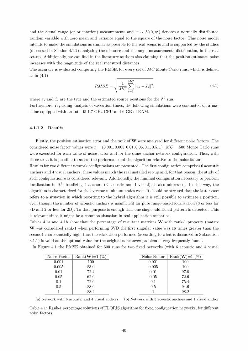
and the actual range (or orientation) measurements and w ∼ N (0, η2) denotes a normally distributedrandom variable with zero mean and variance equal to the square of the noise factor. This noise modelintends to make the simulations as similar as possible to the real scenario and is supported by the studies(discussed in Section 4.1.2) analysing the distance and the angle measurements distribution, in the realset-up. Additionally, we can find in the literature authors also claiming that the position estimates noiseincreases with the magnitude of the real measured distances.The accuracy is evaluated computing the RMSE, for every set of MC Monte Carlo runs, which is definedas in (4.1)

RMSE =

√√√√ 1MC

MC∑i=1‖xi − xi‖2, (4.1)

where xi and xi are the true and the estimated source positions for the ith run.Furthermore, regarding analysis of execution times, the following simulations were conducted on a ma-chine equipped with an Intel i5 1.7 GHz CPU and 6 GB of RAM.

4.1.1.2 Results

Firstly, the position estimation error and the rank of W were analysed for different noise factors. Theconsidered noise factor values were η = (0.001, 0.005, 0.01, 0.05, 0.1, 0.5, 1). MC = 500 Monte Carlo runswere executed for each value of noise factor and for the same anchor network configuration. Thus, withthese tests it is possible to assess the performance of the algorithm relative to the noise factor.Results for two different network configurations are presented. The first configuration comprises 6 acousticanchors and 4 visual anchors, these values match the real installed set-up and, for that reason, the study ofsuch configuration was considered relevant. Additionally, the minimal configuration necessary to performlocalization in R3, totalizing 4 anchors (3 acoustic and 1 visual), is also addressed. In this way, thealgorithm is characterized for the extreme minimum nodes case. It should be stressed that the latter caserefers to a situation in which resorting to the hybrid algorithm it is still possible to estimate a position,even though the number of acoustic anchors is insufficient for pure range-based localization (3 or less for3D and 2 or less for 2D). To that purpose is enough that one single additional pattern is detected. Thisis relevant since it might be a common situation in real application scenarios.Tables 4.1a and 4.1b show that the percentage of resultant matrices W with rank-1 property (matrixW was considered rank-1 when performing SVD the first singular value was 16 times greater than thesecond) is substantially high, thus the relaxation performed (according to what is discussed in Subsection3.1.1) is valid as the optimal value for the original nonconvex problem is very frequently found.

In Figure 4.1 the RMSE obtained for 500 runs for two fixed networks (with 6 acoustic and 4 visual

Noise Factor Rank(W)=1 (%)0.001 1000.005 83.00.01 72.40.05 62.60.1 72.60.5 88.61 88.4

(a) Network with 6 acoustic and 4 visual anchors

Noise Factor Rank(W)=1 (%)0.001 1000.005 1000.01 97.00.05 72.60.1 75.40.5 94.61 98.2

(b) Network with 3 acoustic anchors and 1 visual anchor

Table 4.1: Rank-1 percentage solutions of FLORIS algorithm for fixed configuration networks, for differentnoise factors

40

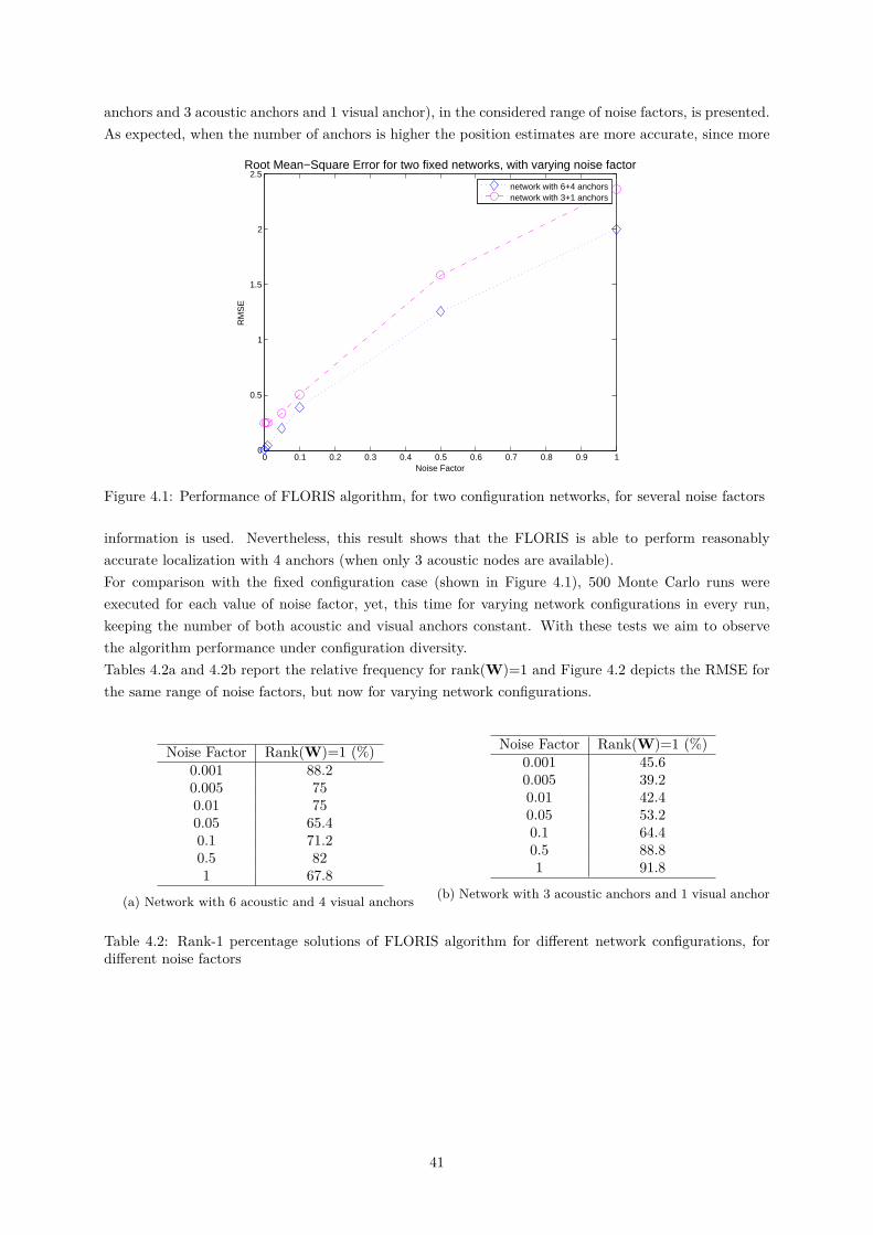
anchors and 3 acoustic anchors and 1 visual anchor), in the considered range of noise factors, is presented.As expected, when the number of anchors is higher the position estimates are more accurate, since more

0 0.1 0.2 0.3 0.4 0.5 0.6 0.7 0.8 0.9 10

0.5

1

1.5

2

2.5

RM

SE

Noise Factor

Root Mean−Square Error for two fixed networks, with varying noise factor

network with 6+4 anchorsnetwork with 3+1 anchors

Figure 4.1: Performance of FLORIS algorithm, for two configuration networks, for several noise factors

information is used. Nevertheless, this result shows that the FLORIS is able to perform reasonablyaccurate localization with 4 anchors (when only 3 acoustic nodes are available).For comparison with the fixed configuration case (shown in Figure 4.1), 500 Monte Carlo runs wereexecuted for each value of noise factor, yet, this time for varying network configurations in every run,keeping the number of both acoustic and visual anchors constant. With these tests we aim to observethe algorithm performance under configuration diversity.Tables 4.2a and 4.2b report the relative frequency for rank(W)=1 and Figure 4.2 depicts the RMSE forthe same range of noise factors, but now for varying network configurations.

Noise Factor Rank(W)=1 (%)0.001 88.20.005 750.01 750.05 65.40.1 71.20.5 821 67.8

(a) Network with 6 acoustic and 4 visual anchors

Noise Factor Rank(W)=1 (%)0.001 45.60.005 39.20.01 42.40.05 53.20.1 64.40.5 88.81 91.8

(b) Network with 3 acoustic anchors and 1 visual anchor

Table 4.2: Rank-1 percentage solutions of FLORIS algorithm for different network configurations, fordifferent noise factors

41

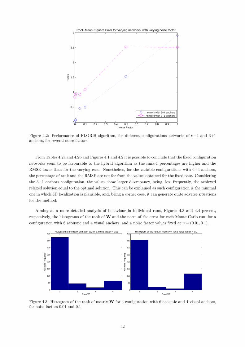
0 0.1 0.2 0.3 0.4 0.5 0.6 0.7 0.8 0.9 10

0.5

1

1.5

2

2.5

3

RM

SE

Noise Factor

Root−Mean−Square Error for varying networks, with varying noise factor

network with 6+4 anchorsnetwork with 3+1 anchors

Figure 4.2: Performance of FLORIS algorithm, for different configurations networks of 6+4 and 3+1anchors, for several noise factors

From Tables 4.2a and 4.2b and Figures 4.1 and 4.2 it is possible to conclude that the fixed configurationnetworks seem to be favourable to the hybrid algorithm as the rank-1 percentages are higher and theRMSE lower than for the varying case. Nonetheless, for the variable configurations with 6+4 anchors,the percentage of rank and the RMSE are not far from the values obtained for the fixed case. Consideringthe 3+1 anchors configuration, the values show larger discrepancy, being, less frequently, the achievedrelaxed solution equal to the optimal solution. This can be explained as such configuration is the minimalone in which 3D localization is plausible, and, being a corner case, it can generate quite adverse situationsfor the method.

Aiming at a more detailed analysis of behaviour in individual runs, Figures 4.3 and 4.4 present,respectively, the histograms of the rank of W and the norm of the error for each Monte Carlo run, for aconfiguration with 6 acoustic and 4 visual anchors, and a noise factor values fixed at η = (0.01, 0.1).

1 2 3 40

50

100

150

200

250

300

350

400

Rank(W)

Abs

olut

e F

requ

ency

Histogram of the rank of matrix W, for a noise factor = 0.01

1 2 3 40

50

100

150

200

250

300

350

400

Rank(W)

Abs

olut

e F

requ

ency

Histogram of the rank of matrix W, for a noise factor = 0.1

Figure 4.3: Histogram of the rank of matrix W for a configuration with 6 acoustic and 4 visual anchors,for noise factors 0.01 and 0.1

42

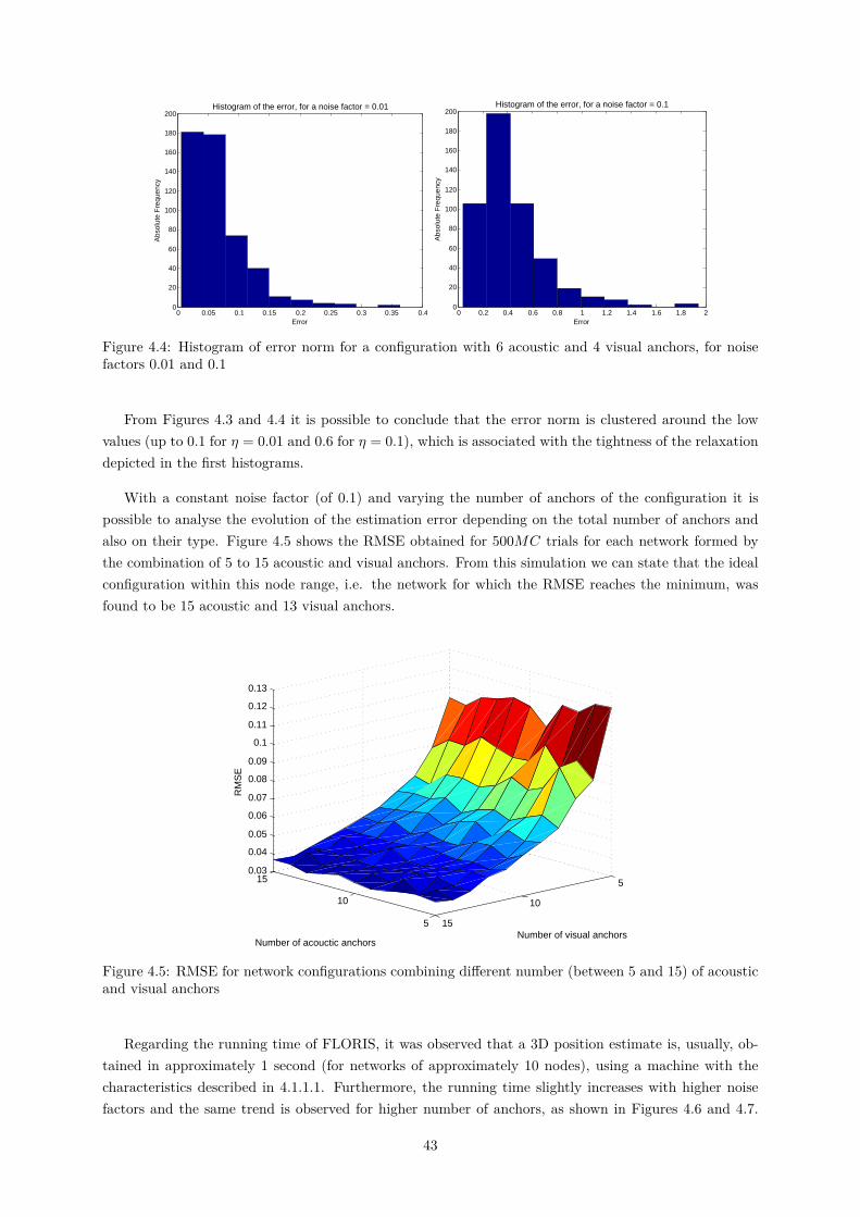
0 0.05 0.1 0.15 0.2 0.25 0.3 0.35 0.40

20

40

60

80

100

120

140

160

180

200

Error

Abs

olut

e F

requ

ency

Histogram of the error, for a noise factor = 0.01

0 0.2 0.4 0.6 0.8 1 1.2 1.4 1.6 1.8 20

20

40

60

80

100

120

140

160

180

200

Error

Abs

olut

e F

requ

ency

Histogram of the error, for a noise factor = 0.1

Figure 4.4: Histogram of error norm for a configuration with 6 acoustic and 4 visual anchors, for noisefactors 0.01 and 0.1

From Figures 4.3 and 4.4 it is possible to conclude that the error norm is clustered around the lowvalues (up to 0.1 for η = 0.01 and 0.6 for η = 0.1), which is associated with the tightness of the relaxationdepicted in the first histograms.

With a constant noise factor (of 0.1) and varying the number of anchors of the configuration it ispossible to analyse the evolution of the estimation error depending on the total number of anchors andalso on their type. Figure 4.5 shows the RMSE obtained for 500MC trials for each network formed bythe combination of 5 to 15 acoustic and visual anchors. From this simulation we can state that the idealconfiguration within this node range, i.e. the network for which the RMSE reaches the minimum, wasfound to be 15 acoustic and 13 visual anchors.

5

10

15 5

10

15

0.03

0.04

0.05

0.06

0.07

0.08

0.09

0.1

0.11

0.12

0.13

Number of visual anchorsNumber of acouctic anchors

RM

SE

Figure 4.5: RMSE for network configurations combining different number (between 5 and 15) of acousticand visual anchors

Regarding the running time of FLORIS, it was observed that a 3D position estimate is, usually, ob-tained in approximately 1 second (for networks of approximately 10 nodes), using a machine with thecharacteristics described in 4.1.1.1. Furthermore, the running time slightly increases with higher noisefactors and the same trend is observed for higher number of anchors, as shown in Figures 4.6 and 4.7.

43

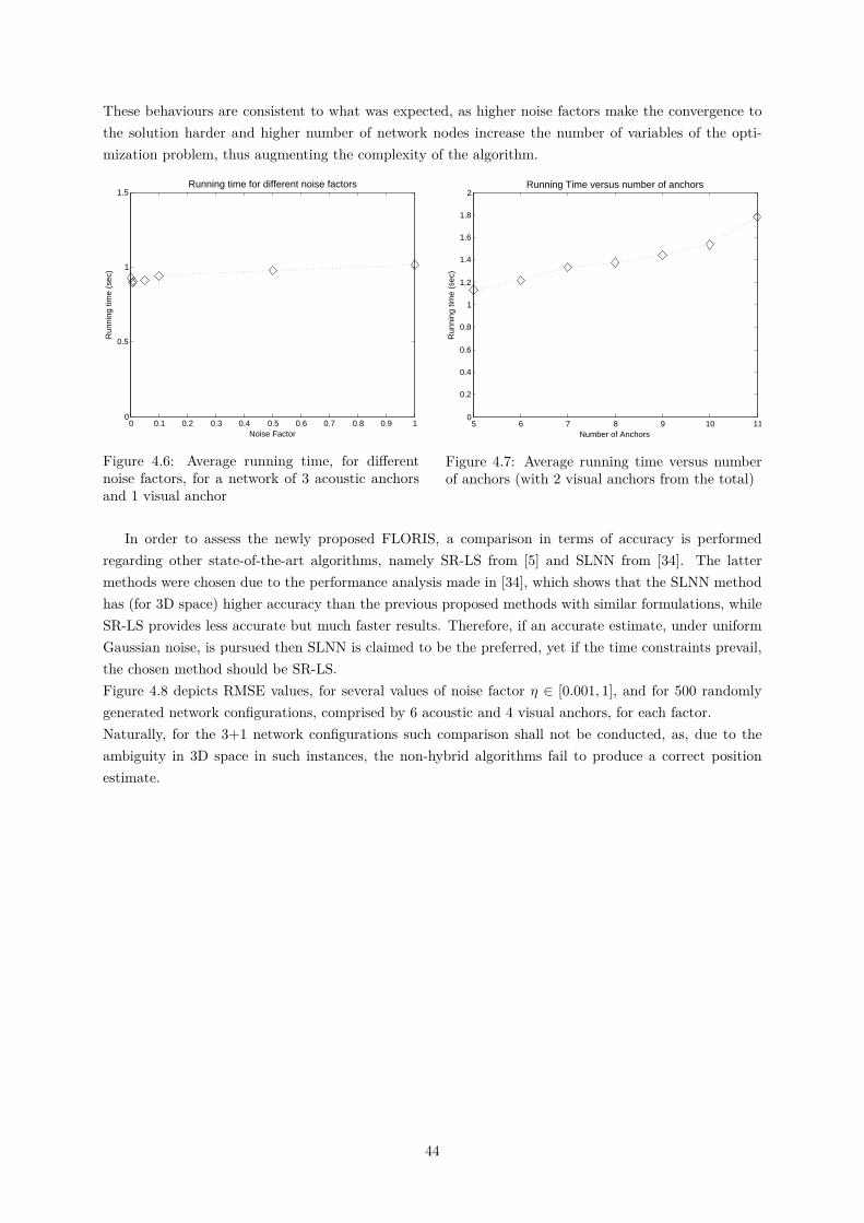
These behaviours are consistent to what was expected, as higher noise factors make the convergence tothe solution harder and higher number of network nodes increase the number of variables of the opti-mization problem, thus augmenting the complexity of the algorithm.

0 0.1 0.2 0.3 0.4 0.5 0.6 0.7 0.8 0.9 10

0.5

1

1.5

Run

ning

tim

e (s

ec)

Noise Factor

Running time for different noise factors

Figure 4.6: Average running time, for differentnoise factors, for a network of 3 acoustic anchorsand 1 visual anchor

5 6 7 8 9 10 110

0.2

0.4

0.6

0.8

1

1.2

1.4

1.6

1.8

2

Run

ning

tim

e (s

ec)

Number of Anchors

Running Time versus number of anchors

Figure 4.7: Average running time versus numberof anchors (with 2 visual anchors from the total)

In order to assess the newly proposed FLORIS, a comparison in terms of accuracy is performedregarding other state-of-the-art algorithms, namely SR-LS from [5] and SLNN from [34]. The lattermethods were chosen due to the performance analysis made in [34], which shows that the SLNN methodhas (for 3D space) higher accuracy than the previous proposed methods with similar formulations, whileSR-LS provides less accurate but much faster results. Therefore, if an accurate estimate, under uniformGaussian noise, is pursued then SLNN is claimed to be the preferred, yet if the time constraints prevail,the chosen method should be SR-LS.Figure 4.8 depicts RMSE values, for several values of noise factor η ∈ [0.001, 1], and for 500 randomlygenerated network configurations, comprised by 6 acoustic and 4 visual anchors, for each factor.Naturally, for the 3+1 network configurations such comparison shall not be conducted, as, due to theambiguity in 3D space in such instances, the non-hybrid algorithms fail to produce a correct positionestimate.

44

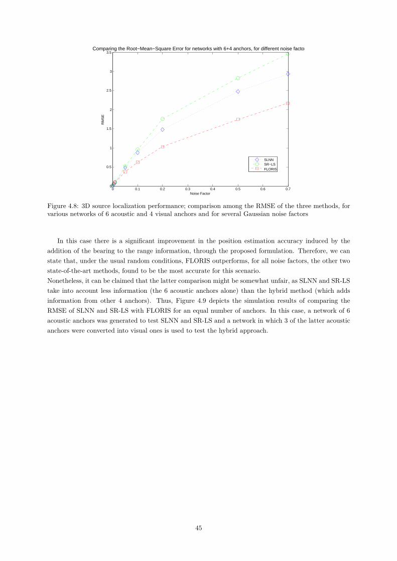
0 0.1 0.2 0.3 0.4 0.5 0.6 0.70

0.5

1

1.5

2

2.5

3

3.5

RM

SE

Noise Factor

Comparing the Root−Mean−Square Error for networks with 6+4 anchors, for different noise factors

SLNNSR−LSFLORIS

Figure 4.8: 3D source localization performance; comparison among the RMSE of the three methods, forvarious networks of 6 acoustic and 4 visual anchors and for several Gaussian noise factors

In this case there is a significant improvement in the position estimation accuracy induced by theaddition of the bearing to the range information, through the proposed formulation. Therefore, we canstate that, under the usual random conditions, FLORIS outperforms, for all noise factors, the other twostate-of-the-art methods, found to be the most accurate for this scenario.Nonetheless, it can be claimed that the latter comparison might be somewhat unfair, as SLNN and SR-LStake into account less information (the 6 acoustic anchors alone) than the hybrid method (which addsinformation from other 4 anchors). Thus, Figure 4.9 depicts the simulation results of comparing theRMSE of SLNN and SR-LS with FLORIS for an equal number of anchors. In this case, a network of 6acoustic anchors was generated to test SLNN and SR-LS and a network in which 3 of the latter acousticanchors were converted into visual ones is used to test the hybrid approach.

45

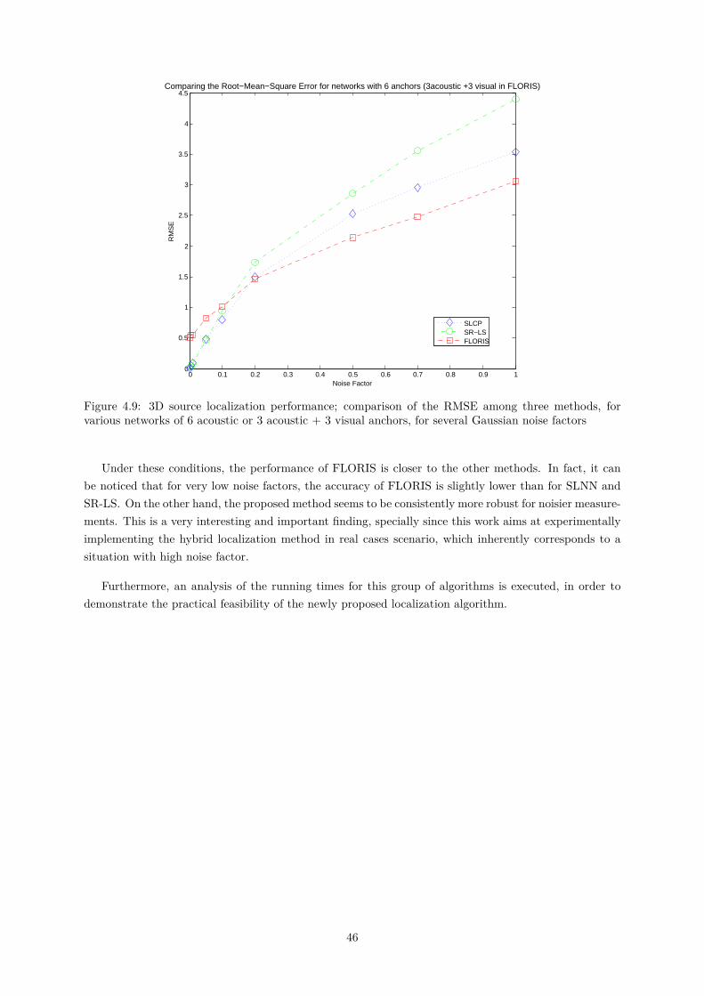
0 0.1 0.2 0.3 0.4 0.5 0.6 0.7 0.8 0.9 10

0.5

1

1.5

2

2.5

3

3.5

4

4.5

RM

SE

Noise Factor

Comparing the Root−Mean−Square Error for networks with 6 anchors (3acoustic +3 visual in FLORIS)

SLCPSR−LSFLORIS

Figure 4.9: 3D source localization performance; comparison of the RMSE among three methods, forvarious networks of 6 acoustic or 3 acoustic + 3 visual anchors, for several Gaussian noise factors

Under these conditions, the performance of FLORIS is closer to the other methods. In fact, it canbe noticed that for very low noise factors, the accuracy of FLORIS is slightly lower than for SLNN andSR-LS. On the other hand, the proposed method seems to be consistently more robust for noisier measure-ments. This is a very interesting and important finding, specially since this work aims at experimentallyimplementing the hybrid localization method in real cases scenario, which inherently corresponds to asituation with high noise factor.

Furthermore, an analysis of the running times for this group of algorithms is executed, in order todemonstrate the practical feasibility of the newly proposed localization algorithm.

46

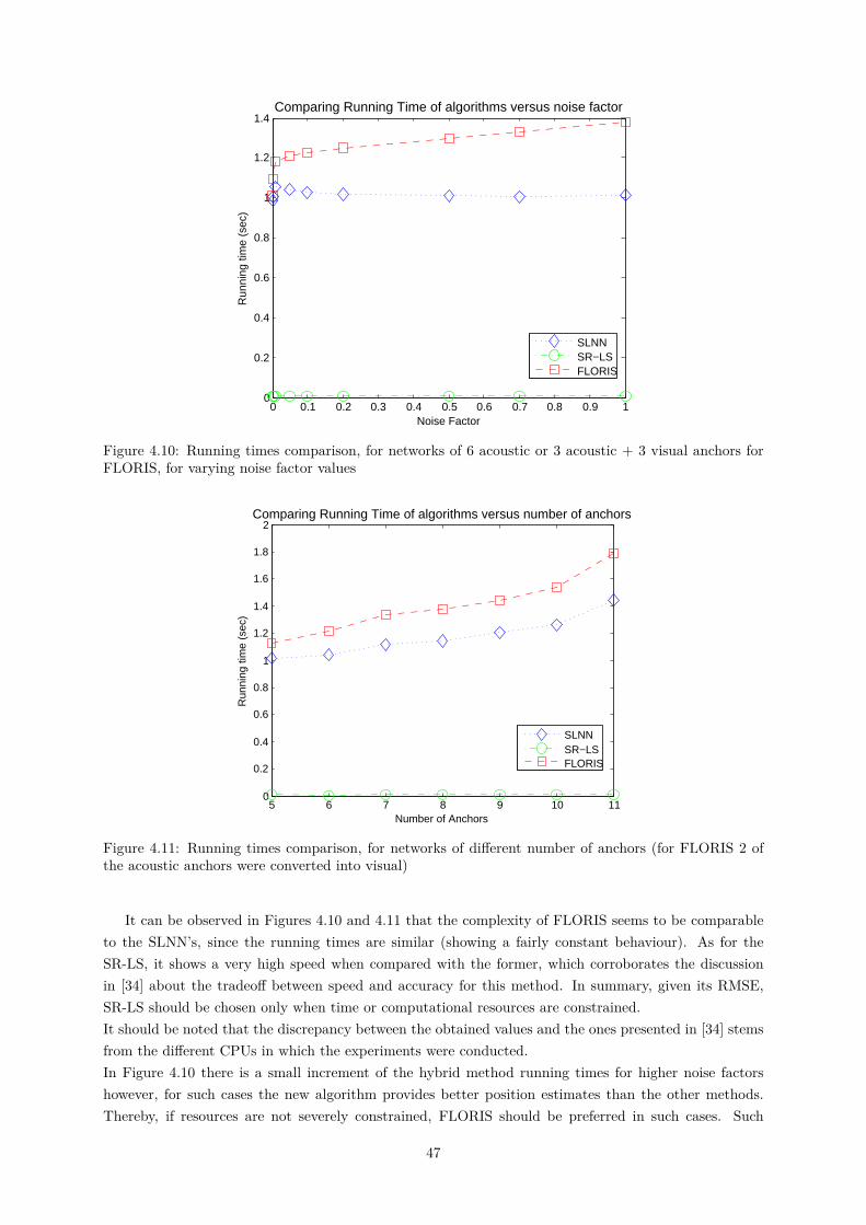
0 0.1 0.2 0.3 0.4 0.5 0.6 0.7 0.8 0.9 10

0.2

0.4

0.6

0.8

1

1.2

1.4

Run

ning

tim

e (s

ec)

Noise Factor

Comparing Running Time of algorithms versus noise factor

SLNNSR−LSFLORIS

Figure 4.10: Running times comparison, for networks of 6 acoustic or 3 acoustic + 3 visual anchors forFLORIS, for varying noise factor values

5 6 7 8 9 10 110

0.2

0.4

0.6

0.8

1

1.2

1.4

1.6

1.8

2

Run

ning

tim

e (s

ec)

Number of Anchors

Comparing Running Time of algorithms versus number of anchors

SLNNSR−LSFLORIS

Figure 4.11: Running times comparison, for networks of different number of anchors (for FLORIS 2 ofthe acoustic anchors were converted into visual)

It can be observed in Figures 4.10 and 4.11 that the complexity of FLORIS seems to be comparableto the SLNN’s, since the running times are similar (showing a fairly constant behaviour). As for theSR-LS, it shows a very high speed when compared with the former, which corroborates the discussionin [34] about the tradeoff between speed and accuracy for this method. In summary, given its RMSE,SR-LS should be chosen only when time or computational resources are constrained.It should be noted that the discrepancy between the obtained values and the ones presented in [34] stemsfrom the different CPUs in which the experiments were conducted.In Figure 4.10 there is a small increment of the hybrid method running times for higher noise factorshowever, for such cases the new algorithm provides better position estimates than the other methods.Thereby, if resources are not severely constrained, FLORIS should be preferred in such cases. Such

47

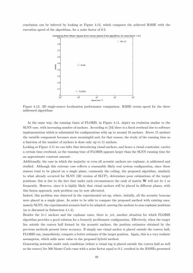
conclusion can be inferred by looking at Figure 4.12, which compares the achieved RMSE with theexecution speed of the algorithms, for a noise factor of 0.2.

10−1 100 101 102 1032

2.1

2.2

2.3

2.4

2.5

2.6

2.7

2.8

2.9

FLORIS

SR−LS

SLNN

RM

SE

Speed (sec−1)

Comparing Root−Mean−Square Error versus Speed of the algorithms, for noise factor = 0.2

Figure 4.12: 3D single-source localization performance comparison: RMSE versus speed for the threeaddressed algorithms

In the same way, the running times of FLORIS, in Figure 4.11, depict an evolution similar to theSLNN case, with increasing number of anchors. According to [34] there is a fixed overhead due to softwareimplementation which is substantial for configurations with up to around 10 anchors. Above 15 anchorsthe variable component becomes more meaningful and, for that reason, the study of the running time asa function of the number of anchors is done only up to 11 anchors.Looking at Figure 4.11 we can infer that introducing visual anchors, and hence a visual constraint, carriesa certain time overhead, as the running time of FLORIS appears larger than the SLNN running time foran approximate constant amount.Additionally, the case in which the majority or even all acoustic anchors are coplanar, is addressed andstudied. Although this extreme case reflects a reasonably likely real system configuration, since thesesensors tend to be placed on a single plane, commonly the ceiling, the proposed algorithm, similarlyto what already occurred for SLNN (3D version of SLCP), determines poor estimations of the targetpositions; this is due to the fact that under such circumstances the rank of matrix W will not be 1 sofrequently. However, since it is highly likely that visual anchors will be placed in different planes, withthis fusion approach, such problem can be now alleviated.Indeed, this problem was observed in the experimental set-up, where, initially, all the acoustic beaconswere placed in a single plane. In order to be able to compare the proposed method with existing ones,namely SLNN, the experimental scenario had to be adapted, moving the anchors to non-coplanar positions(as is discussed in Subsection 4.1.2).Besides the 3+1 anchors and the coplanar cases, there is, yet, another situation for which FLORISalgorithm provides a good solution for a formerly problematic configuration. Effectively, when the targetlies outside the convex hull formed by the acoustic anchors, the position estimates obtained by theprevious methods present lower accuracy. If simply one visual anchor is placed outside the convex hull,FLORIS can, immediately, compute a better estimate of the target position. Again, this is a very realisticassumption, which adds more value to the proposed hybrid method.Generating networks under such conditions (where a visual tag is placed outside the convex hull as wellas the source) for 500 Monte Carlo runs with a noise factor equal to 0.1, resulted in the RMSEs presented

48

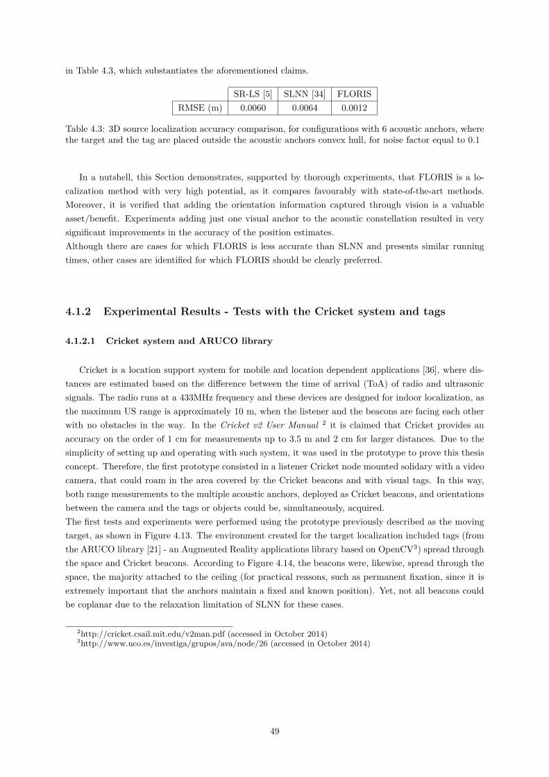
in Table 4.3, which substantiates the aforementioned claims.

SR-LS [5] SLNN [34] FLORISRMSE (m) 0.0060 0.0064 0.0012

Table 4.3: 3D source localization accuracy comparison, for configurations with 6 acoustic anchors, wherethe target and the tag are placed outside the acoustic anchors convex hull, for noise factor equal to 0.1

In a nutshell, this Section demonstrates, supported by thorough experiments, that FLORIS is a lo-calization method with very high potential, as it compares favourably with state-of-the-art methods.Moreover, it is verified that adding the orientation information captured through vision is a valuableasset/benefit. Experiments adding just one visual anchor to the acoustic constellation resulted in verysignificant improvements in the accuracy of the position estimates.Although there are cases for which FLORIS is less accurate than SLNN and presents similar runningtimes, other cases are identified for which FLORIS should be clearly preferred.

4.1.2 Experimental Results - Tests with the Cricket system and tags

4.1.2.1 Cricket system and ARUCO library

Cricket is a location support system for mobile and location dependent applications [36], where dis-tances are estimated based on the difference between the time of arrival (ToA) of radio and ultrasonicsignals. The radio runs at a 433MHz frequency and these devices are designed for indoor localization, asthe maximum US range is approximately 10 m, when the listener and the beacons are facing each otherwith no obstacles in the way. In the Cricket v2 User Manual 2 it is claimed that Cricket provides anaccuracy on the order of 1 cm for measurements up to 3.5 m and 2 cm for larger distances. Due to thesimplicity of setting up and operating with such system, it was used in the prototype to prove this thesisconcept. Therefore, the first prototype consisted in a listener Cricket node mounted solidary with a videocamera, that could roam in the area covered by the Cricket beacons and with visual tags. In this way,both range measurements to the multiple acoustic anchors, deployed as Cricket beacons, and orientationsbetween the camera and the tags or objects could be, simultaneously, acquired.The first tests and experiments were performed using the prototype previously described as the movingtarget, as shown in Figure 4.13. The environment created for the target localization included tags (fromthe ARUCO library [21] - an Augmented Reality applications library based on OpenCV3) spread throughthe space and Cricket beacons. According to Figure 4.14, the beacons were, likewise, spread through thespace, the majority attached to the ceiling (for practical reasons, such as permanent fixation, since it isextremely important that the anchors maintain a fixed and known position). Yet, not all beacons couldbe coplanar due to the relaxation limitation of SLNN for these cases.

2http://cricket.csail.mit.edu/v2man.pdf (accessed in October 2014)3http://www.uco.es/investiga/grupos/ava/node/26 (accessed in October 2014)

49

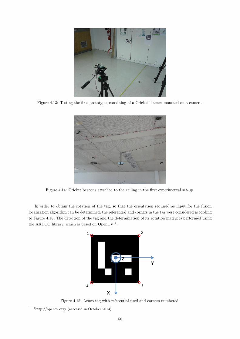
Figure 4.13: Testing the first prototype, consisting of a Cricket listener mounted on a camera

Figure 4.14: Cricket beacons attached to the ceiling in the first experimental set-up

In order to obtain the rotation of the tag, so that the orientation required as input for the fusionlocalization algorithm can be determined, the referential and corners in the tag were considered accordingto Figure 4.15. The detection of the tag and the determination of its rotation matrix is performed usingthe ARUCO library, which is based on OpenCV 4.

Y

X

Z

1 2

34

Figure 4.15: Aruco tag with referential used and corners numbered4http://opencv.org/ (accessed in October 2014)

50

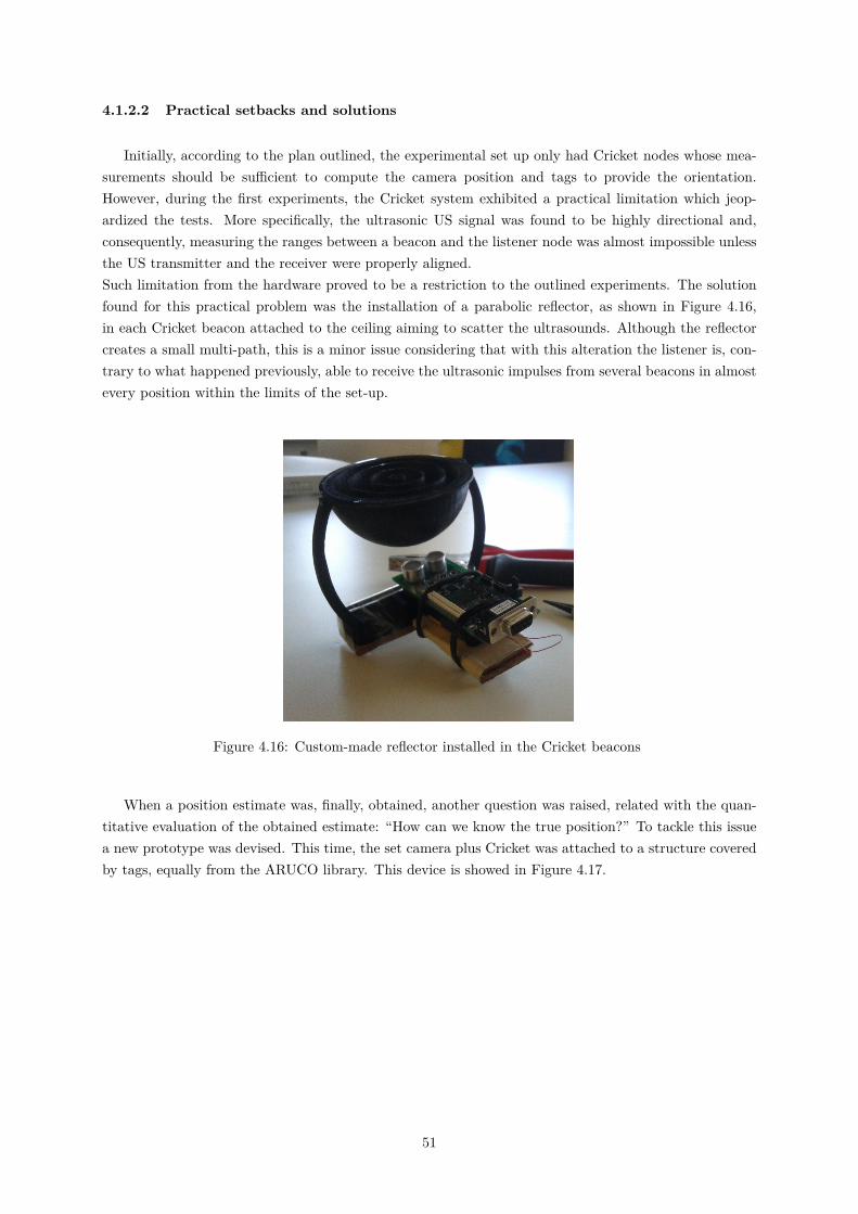
4.1.2.2 Practical setbacks and solutions

Initially, according to the plan outlined, the experimental set up only had Cricket nodes whose mea-surements should be sufficient to compute the camera position and tags to provide the orientation.However, during the first experiments, the Cricket system exhibited a practical limitation which jeop-ardized the tests. More specifically, the ultrasonic US signal was found to be highly directional and,consequently, measuring the ranges between a beacon and the listener node was almost impossible unlessthe US transmitter and the receiver were properly aligned.Such limitation from the hardware proved to be a restriction to the outlined experiments. The solutionfound for this practical problem was the installation of a parabolic reflector, as shown in Figure 4.16,in each Cricket beacon attached to the ceiling aiming to scatter the ultrasounds. Although the reflectorcreates a small multi-path, this is a minor issue considering that with this alteration the listener is, con-trary to what happened previously, able to receive the ultrasonic impulses from several beacons in almostevery position within the limits of the set-up.

Figure 4.16: Custom-made reflector installed in the Cricket beacons

When a position estimate was, finally, obtained, another question was raised, related with the quan-titative evaluation of the obtained estimate: “How can we know the true position?” To tackle this issuea new prototype was devised. This time, the set camera plus Cricket was attached to a structure coveredby tags, equally from the ARUCO library. This device is showed in Figure 4.17.

51

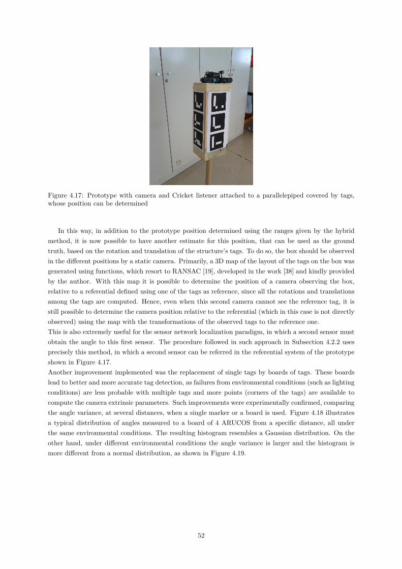
Figure 4.17: Prototype with camera and Cricket listener attached to a parallelepiped covered by tags,whose position can be determined

In this way, in addition to the prototype position determined using the ranges given by the hybridmethod, it is now possible to have another estimate for this position, that can be used as the groundtruth, based on the rotation and translation of the structure’s tags. To do so, the box should be observedin the different positions by a static camera. Primarily, a 3D map of the layout of the tags on the box wasgenerated using functions, which resort to RANSAC [19], developed in the work [38] and kindly providedby the author. With this map it is possible to determine the position of a camera observing the box,relative to a referential defined using one of the tags as reference, since all the rotations and translationsamong the tags are computed. Hence, even when this second camera cannot see the reference tag, it isstill possible to determine the camera position relative to the referential (which in this case is not directlyobserved) using the map with the transformations of the observed tags to the reference one.This is also extremely useful for the sensor network localization paradigm, in which a second sensor mustobtain the angle to this first sensor. The procedure followed in such approach in Subsection 4.2.2 usesprecisely this method, in which a second sensor can be referred in the referential system of the prototypeshown in Figure 4.17.Another improvement implemented was the replacement of single tags by boards of tags. These boardslead to better and more accurate tag detection, as failures from environmental conditions (such as lightingconditions) are less probable with multiple tags and more points (corners of the tags) are available tocompute the camera extrinsic parameters. Such improvements were experimentally confirmed, comparingthe angle variance, at several distances, when a single marker or a board is used. Figure 4.18 illustratesa typical distribution of angles measured to a board of 4 ARUCOS from a specific distance, all underthe same environmental conditions. The resulting histogram resembles a Gaussian distribution. On theother hand, under different environmental conditions the angle variance is larger and the histogram ismore different from a normal distribution, as shown in Figure 4.19.

52

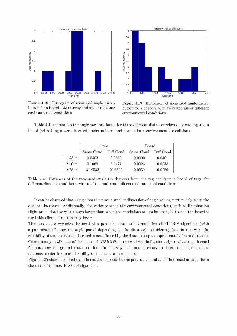
179 179.05 179.1 179.15 179.2 179.25 179.3 179.35 179.4 179.450

0.5

1

1.5

2

2.5

3Histogram of angle distribution

Angle (deg)

Abs

oltu

e fr

eque

ncy

Figure 4.18: Histogram of measured angle distri-bution for a board 1.53 m away and under the sameenvironmental conditions

170.2 170.3 170.4 170.5 170.6 170.7 170.80

0.5

1

1.5

2

2.5

3

3.5

4

4.5

5Histogram of angle distribution

Angle (deg)

Abs

oltu

e fr

eque

ncy

Figure 4.19: Histogram of measured angle distri-bution for a board 2.78 m away and under differentenvironmental conditions

Table 4.4 summarizes the angle variance found for three different distances when only one tag and aboard (with 4 tags) were detected, under uniform and non-uniform environmental conditions.

1 tag BoardSame Cond Diff Cond Same Cond Diff Cond

1.53 m 0.0403 0.0669 0.0090 0.04012.10 m 0.1069 8.0474 0.0023 0.02382.78 m 31.9533 20.6532 0.0052 0.0286

Table 4.4: Variances of the measured angle (in degrees) from one tag and from a board of tags, fordifferent distances and both with uniform and non-uniform environmental conditions

It can be observed that using a board causes a smaller dispersion of angle values, particularly when thedistance increases. Additionally, the variance when the environmental conditions, such as illumination(light or shadow) vary is always larger than when the conditions are maintained, but when the board isused this effect is substantially lower.This study also excludes the need of a possible parametric formulation of FLORIS algorithm (witha parameter affecting the angle parcel depending on the distance), considering that, in this way, thereliability of the orientation detected is not affected by the distance (up to approximately 5m of distance).Consequently, a 3D map of the board of ARUCOS on the wall was built, similarly to what is performedfor obtaining the ground truth position. In this way, it is not necessary to detect the tag defined asreference conferring more flexibility to the camera movements.Figure 4.20 shows the final experimental set-up used to acquire range and angle information to performthe tests of the new FLORIS algorithm.

53

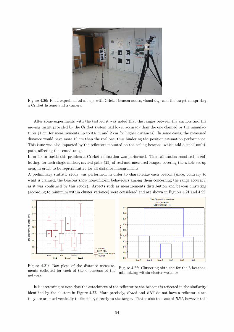
Figure 4.20: Final experimental set-up, with Cricket beacon nodes, visual tags and the target comprisinga Cricket listener and a camera

After some experiments with the testbed it was noted that the ranges between the anchors and themoving target provided by the Cricket system had lower accuracy than the one claimed by the manufac-turer (1 cm for measurements up to 3.5 m and 2 cm for higher distances). In some cases, the measureddistance would have more 10 cm than the real one, thus hindering the position estimation performance.This issue was also impacted by the reflectors mounted on the ceiling beacons, which add a small multi-path, affecting the sensed range.In order to tackle this problem a Cricket calibration was performed. This calibration consisted in col-lecting, for each single anchor, several pairs (25) of real and measured ranges, covering the whole set-uparea, in order to be representative for all distance measurements.A preliminary statistic study was performed, in order to characterize each beacon (since, contrary towhat is claimed, the beacons show non-uniform behaviours among them concerning the range accuracy,as it was confirmed by this study). Aspects such as measurements distribution and beacon clustering(according to minimum within cluster variance) were considered and are shown in Figures 4.21 and 4.22.

Measu

rem

en

t Err

or

(m)

Figure 4.21: Box plots of the distance measure-ments collected for each of the 6 beacons of thenetwork

Figure 4.22: Clustering obtained for the 6 beacons,minimizing within cluster variance

It is interesting to note that the attachment of the reflector to the beacons is reflected in the similarityidentified by the clusters in Figure 4.22. More precisely, Beac2 and BN6 do not have a reflector, sincethey are oriented vertically to the floor, directly to the target. That is also the case of BN1, however this

54

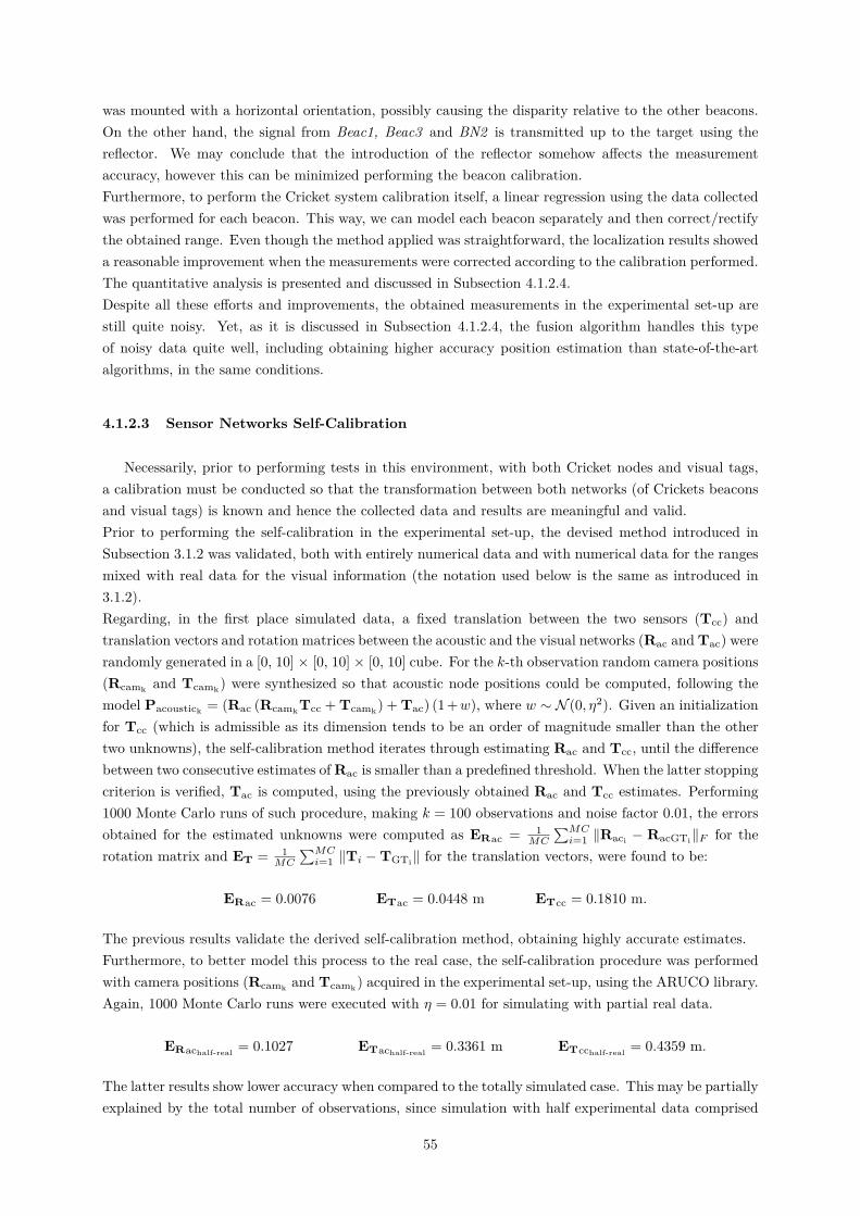
was mounted with a horizontal orientation, possibly causing the disparity relative to the other beacons.On the other hand, the signal from Beac1, Beac3 and BN2 is transmitted up to the target using thereflector. We may conclude that the introduction of the reflector somehow affects the measurementaccuracy, however this can be minimized performing the beacon calibration.Furthermore, to perform the Cricket system calibration itself, a linear regression using the data collectedwas performed for each beacon. This way, we can model each beacon separately and then correct/rectifythe obtained range. Even though the method applied was straightforward, the localization results showeda reasonable improvement when the measurements were corrected according to the calibration performed.The quantitative analysis is presented and discussed in Subsection 4.1.2.4.Despite all these efforts and improvements, the obtained measurements in the experimental set-up arestill quite noisy. Yet, as it is discussed in Subsection 4.1.2.4, the fusion algorithm handles this typeof noisy data quite well, including obtaining higher accuracy position estimation than state-of-the-artalgorithms, in the same conditions.

4.1.2.3 Sensor Networks Self-Calibration

Necessarily, prior to performing tests in this environment, with both Cricket nodes and visual tags,a calibration must be conducted so that the transformation between both networks (of Crickets beaconsand visual tags) is known and hence the collected data and results are meaningful and valid.Prior to performing the self-calibration in the experimental set-up, the devised method introduced inSubsection 3.1.2 was validated, both with entirely numerical data and with numerical data for the rangesmixed with real data for the visual information (the notation used below is the same as introduced in3.1.2).Regarding, in the first place simulated data, a fixed translation between the two sensors (Tcc) andtranslation vectors and rotation matrices between the acoustic and the visual networks (Rac and Tac) wererandomly generated in a [0, 10] × [0, 10] × [0, 10] cube. For the k-th observation random camera positions(Rcamk and Tcamk) were synthesized so that acoustic node positions could be computed, following themodel Pacoustick = (Rac (RcamkTcc + Tcamk) + Tac) (1+w), where w ∼ N (0, η2). Given an initializationfor Tcc (which is admissible as its dimension tends to be an order of magnitude smaller than the othertwo unknowns), the self-calibration method iterates through estimating Rac and Tcc, until the differencebetween two consecutive estimates of Rac is smaller than a predefined threshold. When the latter stoppingcriterion is verified, Tac is computed, using the previously obtained Rac and Tcc estimates. Performing1000 Monte Carlo runs of such procedure, making k = 100 observations and noise factor 0.01, the errorsobtained for the estimated unknowns were computed as ERac = 1

MC

∑MCi=1 ‖Raci − RacGTi‖F for the

rotation matrix and ET = 1MC

∑MCi=1 ‖Ti −TGTi‖ for the translation vectors, were found to be:

ERac = 0.0076 ETac = 0.0448 m ETcc = 0.1810 m.

The previous results validate the derived self-calibration method, obtaining highly accurate estimates.Furthermore, to better model this process to the real case, the self-calibration procedure was performedwith camera positions (Rcamk and Tcamk) acquired in the experimental set-up, using the ARUCO library.Again, 1000 Monte Carlo runs were executed with η = 0.01 for simulating with partial real data.

ERachalf-real = 0.1027 ETachalf-real = 0.3361 m ETcchalf-real = 0.4359 m.

The latter results show lower accuracy when compared to the totally simulated case. This may be partiallyexplained by the total number of observations, since simulation with half experimental data comprised

55

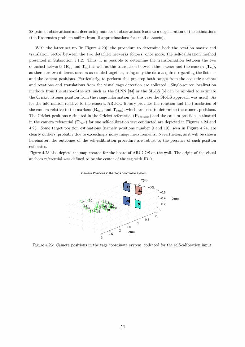
28 pairs of observations and decreasing number of observations leads to a degeneration of the estimations(the Procrustes problem suffers from ill approximations for small datasets).

With the latter set up (in Figure 4.20), the procedure to determine both the rotation matrix andtranslation vector between the two detached networks follows, once more, the self-calibration methodpresented in Subsection 3.1.2. Thus, it is possible to determine the transformation between the twodetached networks (Rac and Tac) as well as the translation between the listener and the camera (Tcc),as there are two different sensors assembled together, using only the data acquired regarding the listenerand the camera positions. Particularly, to perform this pre-step both ranges from the acoustic anchorsand rotations and translations from the visual tags detection are collected. Single-source localizationmethods from the state-of-the art, such as the SLNN [34] or the SR-LS [5] can be applied to estimatethe Cricket listener position from the range information (in this case the SR-LS approach was used). Asfor the information relative to the camera, ARUCO library provides the rotation and the translation ofthe camera relative to the markers (Rcam and Tcam), which are used to determine the camera positions.The Cricket positions estimated in the Cricket referential (Pacoustic) and the camera positions estimatedin the camera referential (Tcam) for one self-calibration test conducted are depicted in Figures 4.24 and4.23. Some target position estimations (namely positions number 9 and 10), seen in Figure 4.24, areclearly outliers, probably due to exceedingly noisy range measurements. Nevertheless, as it will be shownhereinafter, the outcomes of the self-calibration procedure are robust to the presence of such positionestimates.Figure 4.23 also depicts the map created for the board of ARUCOS on the wall. The origin of the visualanchors referential was defined to be the center of the tag with ID 0.

−0.6

−0.4

−0.2

0

−0.50

0.5

00.5

11.5

22.5

3

X(m)

Y(m)

21212121212121212121212121212121212121212121212121212121

0000000000000000000000000000

Z(m)

17171717171717171717171717171717171717171717171717171717

29292929292929292929292929292929292929292929292929292929

Camera Positions in the Tags coordinate system

202292110

23

18

11

192825

12

274

237

5

16

18

1715

26

24613

14

Figure 4.23: Camera positions in the tags coordinate system, collected for the self-calibration input

56

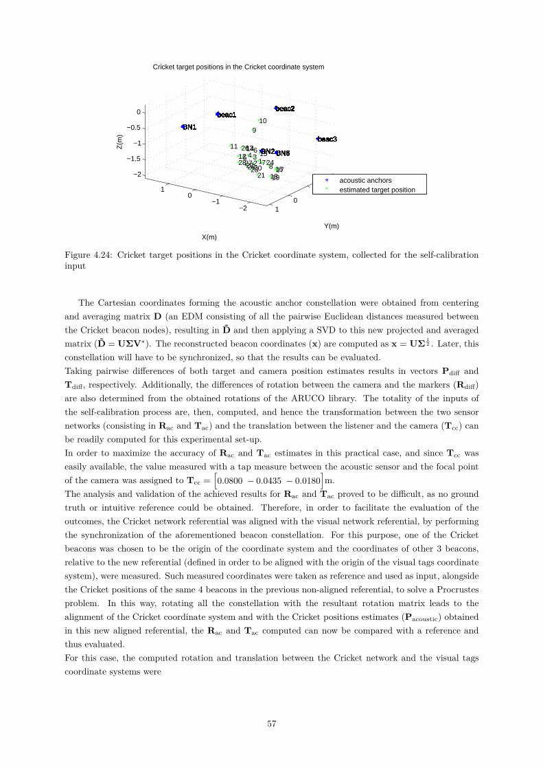
−2−1

01

−2−1

01

−2

−1.5

−1

−0.5

0

Y(m)

beac3beac3beac3beac3beac3beac3beac3beac3beac3beac3beac3beac3beac3beac3beac3beac3beac3beac3beac3beac3beac3beac3beac3

17

BN6 BN6 BN6 BN6 BN6 BN6 BN6 BN6 BN6 BN6 BN6 BN6 BN6 BN6 BN6 BN6 BN6 BN6 BN6 BN6 BN6 BN6 BN6 BN6 BN6 BN6 BN6 BN6

beac2beac2beac2beac2beac2beac2beac2beac2beac2beac2beac2beac2beac2beac2beac2beac2beac2beac2beac2beac2beac2beac2beac2beac2

161918

8247

BN2 BN2 BN2 BN2 BN2 BN2 BN2 BN2 BN2 BN2 BN2 BN2 BN2 BN2 BN2 BN2 BN2 BN2 BN2 BN2 BN2 BN2 BN2 BN2 BN2 BN2 BN2 BN2 15

10

1

21202

63

9

23

4

25

14

22

13

27526

12

Cricket target positions in the Cricket coordinate system

28

11

beac1beac1beac1beac1beac1beac1beac1beac1beac1beac1beac1beac1beac1beac1beac1beac1beac1beac1beac1beac1

X(m)

BN1 BN1 BN1 BN1 BN1 BN1 BN1 BN1 BN1 BN1 BN1 BN1 BN1 BN1 BN1

Z(m

)

acoustic anchorsestimated target position

Figure 4.24: Cricket target positions in the Cricket coordinate system, collected for the self-calibrationinput

The Cartesian coordinates forming the acoustic anchor constellation were obtained from centeringand averaging matrix D (an EDM consisting of all the pairwise Euclidean distances measured betweenthe Cricket beacon nodes), resulting in D and then applying a SVD to this new projected and averagedmatrix (D = UΣV∗). The reconstructed beacon coordinates (x) are computed as x = UΣ 1

2 . Later, thisconstellation will have to be synchronized, so that the results can be evaluated.Taking pairwise differences of both target and camera position estimates results in vectors Pdiff andTdiff, respectively. Additionally, the differences of rotation between the camera and the markers (Rdiff)are also determined from the obtained rotations of the ARUCO library. The totality of the inputs ofthe self-calibration process are, then, computed, and hence the transformation between the two sensornetworks (consisting in Rac and Tac) and the translation between the listener and the camera (Tcc) canbe readily computed for this experimental set-up.In order to maximize the accuracy of Rac and Tac estimates in this practical case, and since Tcc waseasily available, the value measured with a tap measure between the acoustic sensor and the focal pointof the camera was assigned to Tcc =

[0.0800 − 0.0435 − 0.0180

]m.

The analysis and validation of the achieved results for Rac and Tac proved to be difficult, as no groundtruth or intuitive reference could be obtained. Therefore, in order to facilitate the evaluation of theoutcomes, the Cricket network referential was aligned with the visual network referential, by performingthe synchronization of the aforementioned beacon constellation. For this purpose, one of the Cricketbeacons was chosen to be the origin of the coordinate system and the coordinates of other 3 beacons,relative to the new referential (defined in order to be aligned with the origin of the visual tags coordinatesystem), were measured. Such measured coordinates were taken as reference and used as input, alongsidethe Cricket positions of the same 4 beacons in the previous non-aligned referential, to solve a Procrustesproblem. In this way, rotating all the constellation with the resultant rotation matrix leads to thealignment of the Cricket coordinate system and with the Cricket positions estimates (Pacoustic) obtainedin this new aligned referential, the Rac and Tac computed can now be compared with a reference andthus evaluated.For this case, the computed rotation and translation between the Cricket network and the visual tagscoordinate systems were

57

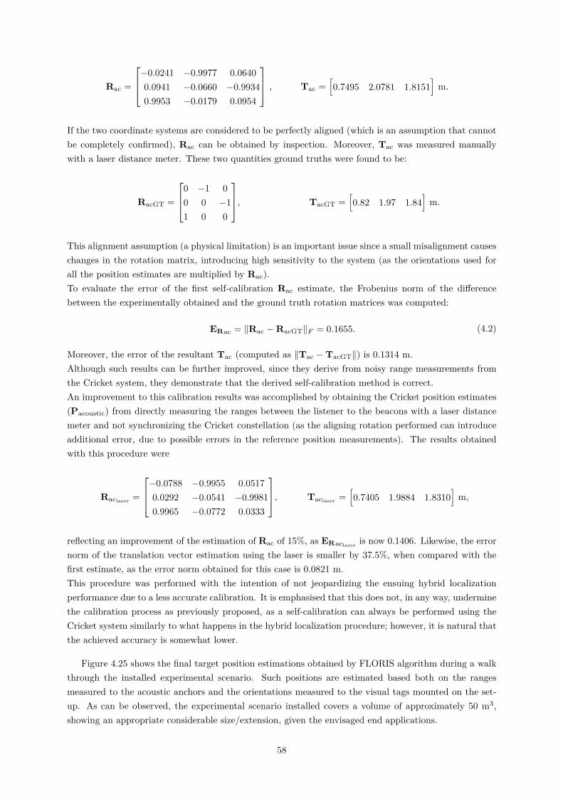
Rac =

−0.0241 −0.9977 0.06400.0941 −0.0660 −0.99340.9953 −0.0179 0.0954

, Tac =[0.7495 2.0781 1.8151

]m.

If the two coordinate systems are considered to be perfectly aligned (which is an assumption that cannotbe completely confirmed), Rac can be obtained by inspection. Moreover, Tac was measured manuallywith a laser distance meter. These two quantities ground truths were found to be:

RacGT =

0 −1 00 0 −11 0 0

, TacGT =[0.82 1.97 1.84

]m.

This alignment assumption (a physical limitation) is an important issue since a small misalignment causeschanges in the rotation matrix, introducing high sensitivity to the system (as the orientations used forall the position estimates are multiplied by Rac).To evaluate the error of the first self-calibration Rac estimate, the Frobenius norm of the differencebetween the experimentally obtained and the ground truth rotation matrices was computed:

ERac = ‖Rac −RacGT‖F = 0.1655. (4.2)

Moreover, the error of the resultant Tac (computed as ‖Tac −TacGT‖) is 0.1314 m.Although such results can be further improved, since they derive from noisy range measurements fromthe Cricket system, they demonstrate that the derived self-calibration method is correct.An improvement to this calibration results was accomplished by obtaining the Cricket position estimates(Pacoustic) from directly measuring the ranges between the listener to the beacons with a laser distancemeter and not synchronizing the Cricket constellation (as the aligning rotation performed can introduceadditional error, due to possible errors in the reference position measurements). The results obtainedwith this procedure were

Raclaser =

−0.0788 −0.9955 0.05170.0292 −0.0541 −0.99810.9965 −0.0772 0.0333

, Taclaser =[0.7405 1.9884 1.8310

]m,

reflecting an improvement of the estimation of Rac of 15%, as ERaclaser is now 0.1406. Likewise, the errornorm of the translation vector estimation using the laser is smaller by 37.5%, when compared with thefirst estimate, as the error norm obtained for this case is 0.0821 m.This procedure was performed with the intention of not jeopardizing the ensuing hybrid localizationperformance due to a less accurate calibration. It is emphasised that this does not, in any way, underminethe calibration process as previously proposed, as a self-calibration can always be performed using theCricket system similarly to what happens in the hybrid localization procedure; however, it is natural thatthe achieved accuracy is somewhat lower.

Figure 4.25 shows the final target position estimations obtained by FLORIS algorithm during a walkthrough the installed experimental scenario. Such positions are estimated based both on the rangesmeasured to the acoustic anchors and the orientations measured to the visual tags mounted on the set-up. As can be observed, the experimental scenario installed covers a volume of approximately 50 m3,showing an appropriate considerable size/extension, given the envisaged end applications.

58

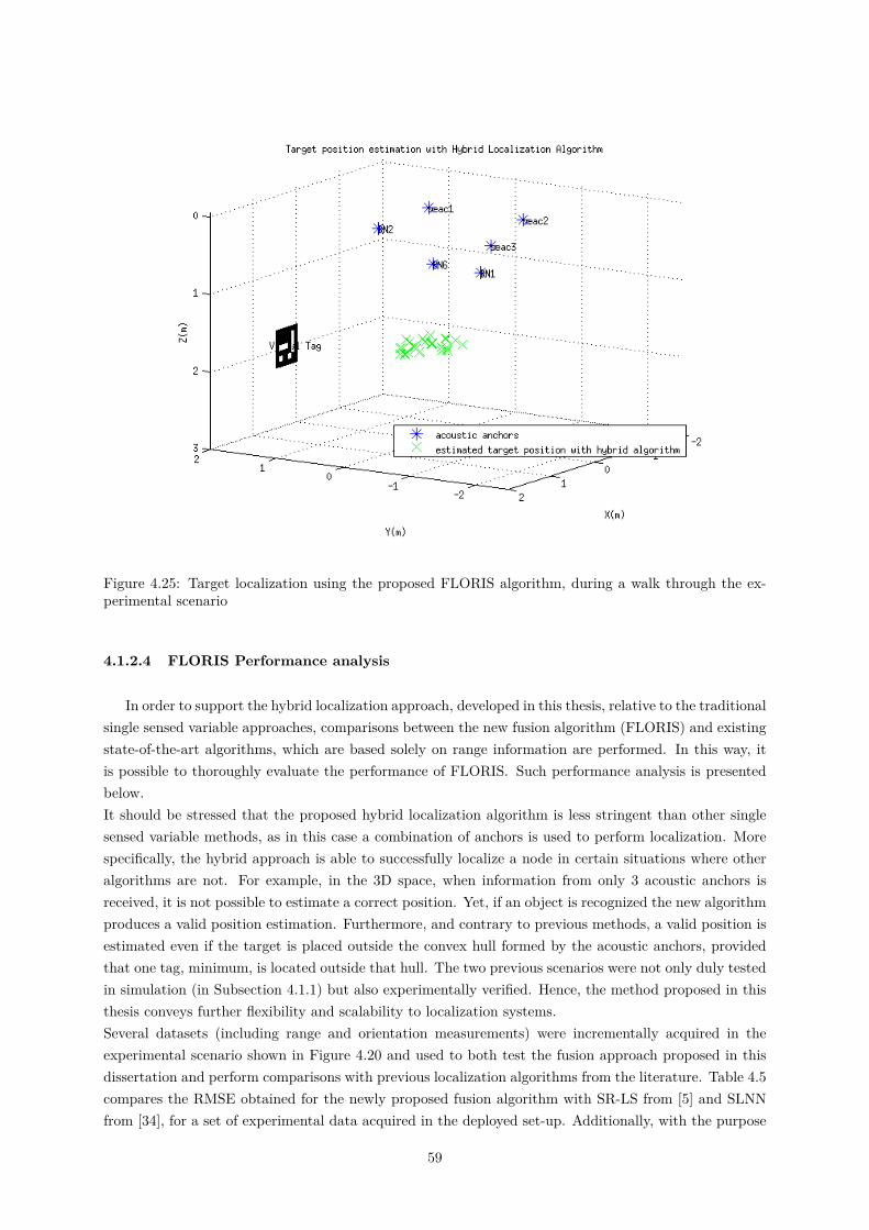
Figure 4.25: Target localization using the proposed FLORIS algorithm, during a walk through the ex-perimental scenario

4.1.2.4 FLORIS Performance analysis

In order to support the hybrid localization approach, developed in this thesis, relative to the traditionalsingle sensed variable approaches, comparisons between the new fusion algorithm (FLORIS) and existingstate-of-the-art algorithms, which are based solely on range information are performed. In this way, itis possible to thoroughly evaluate the performance of FLORIS. Such performance analysis is presentedbelow.It should be stressed that the proposed hybrid localization algorithm is less stringent than other singlesensed variable methods, as in this case a combination of anchors is used to perform localization. Morespecifically, the hybrid approach is able to successfully localize a node in certain situations where otheralgorithms are not. For example, in the 3D space, when information from only 3 acoustic anchors isreceived, it is not possible to estimate a correct position. Yet, if an object is recognized the new algorithmproduces a valid position estimation. Furthermore, and contrary to previous methods, a valid position isestimated even if the target is placed outside the convex hull formed by the acoustic anchors, providedthat one tag, minimum, is located outside that hull. The two previous scenarios were not only duly testedin simulation (in Subsection 4.1.1) but also experimentally verified. Hence, the method proposed in thisthesis conveys further flexibility and scalability to localization systems.Several datasets (including range and orientation measurements) were incrementally acquired in theexperimental scenario shown in Figure 4.20 and used to both test the fusion approach proposed in thisdissertation and perform comparisons with previous localization algorithms from the literature. Table 4.5compares the RMSE obtained for the newly proposed fusion algorithm with SR-LS from [5] and SLNNfrom [34], for a set of experimental data acquired in the deployed set-up. Additionally, with the purpose

59

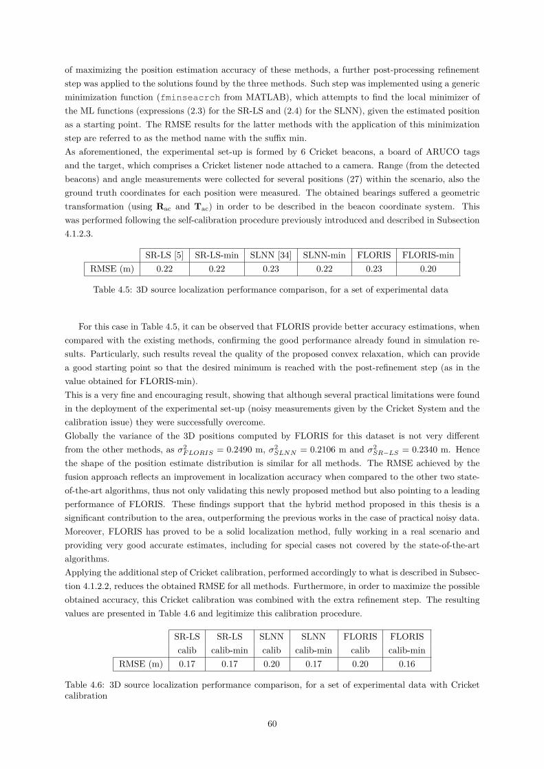
of maximizing the position estimation accuracy of these methods, a further post-processing refinementstep was applied to the solutions found by the three methods. Such step was implemented using a genericminimization function (fminseacrch from MATLAB), which attempts to find the local minimizer ofthe ML functions (expressions (2.3) for the SR-LS and (2.4) for the SLNN), given the estimated positionas a starting point. The RMSE results for the latter methods with the application of this minimizationstep are referred to as the method name with the suffix min.As aforementioned, the experimental set-up is formed by 6 Cricket beacons, a board of ARUCO tagsand the target, which comprises a Cricket listener node attached to a camera. Range (from the detectedbeacons) and angle measurements were collected for several positions (27) within the scenario, also theground truth coordinates for each position were measured. The obtained bearings suffered a geometrictransformation (using Rac and Tac) in order to be described in the beacon coordinate system. Thiswas performed following the self-calibration procedure previously introduced and described in Subsection4.1.2.3.

SR-LS [5] SR-LS-min SLNN [34] SLNN-min FLORIS FLORIS-minRMSE (m) 0.22 0.22 0.23 0.22 0.23 0.20

Table 4.5: 3D source localization performance comparison, for a set of experimental data

For this case in Table 4.5, it can be observed that FLORIS provide better accuracy estimations, whencompared with the existing methods, confirming the good performance already found in simulation re-sults. Particularly, such results reveal the quality of the proposed convex relaxation, which can providea good starting point so that the desired minimum is reached with the post-refinement step (as in thevalue obtained for FLORIS-min).This is a very fine and encouraging result, showing that although several practical limitations were foundin the deployment of the experimental set-up (noisy measurements given by the Cricket System and thecalibration issue) they were successfully overcome.Globally the variance of the 3D positions computed by FLORIS for this dataset is not very differentfrom the other methods, as σ2

FLORIS = 0.2490 m, σ2SLNN = 0.2106 m and σ2

SR−LS = 0.2340 m. Hencethe shape of the position estimate distribution is similar for all methods. The RMSE achieved by thefusion approach reflects an improvement in localization accuracy when compared to the other two state-of-the-art algorithms, thus not only validating this newly proposed method but also pointing to a leadingperformance of FLORIS. These findings support that the hybrid method proposed in this thesis is asignificant contribution to the area, outperforming the previous works in the case of practical noisy data.Moreover, FLORIS has proved to be a solid localization method, fully working in a real scenario andproviding very good accurate estimates, including for special cases not covered by the state-of-the-artalgorithms.Applying the additional step of Cricket calibration, performed accordingly to what is described in Subsec-tion 4.1.2.2, reduces the obtained RMSE for all methods. Furthermore, in order to maximize the possibleobtained accuracy, this Cricket calibration was combined with the extra refinement step. The resultingvalues are presented in Table 4.6 and legitimize this calibration procedure.

SR-LS SR-LS SLNN SLNN FLORIS FLORIScalib calib-min calib calib-min calib calib-min

RMSE (m) 0.17 0.17 0.20 0.17 0.20 0.16

Table 4.6: 3D source localization performance comparison, for a set of experimental data with Cricketcalibration

60

Figure 4.26 shows the histogram of the absolute error for the FLORIS estimates, from which the lowerror of the majority of the position estimates can be perceived.

0.1 0.2 0.3 0.4 0.5 0.6 0.7 0.80

1

2

3

4

5

6

7

8Absolute error of FLORIS experimental position estimates

m

Figure 4.26: Histogram of the absolute error of target positions estimated by FLORIS during a walkthrough the experimental set-up

Figure 4.27 depicts the target positions estimated by FLORIS algorithm versus the ground truthpositions. It can be observed that the estimated positions are, globally, very close to the ground truth,indicating a reasonable and promising accuracy.

Figure 4.27: Target position estimations given by FLORIS algorithm, during a walk through the experi-mental scenario, versus the ground truth positions

61

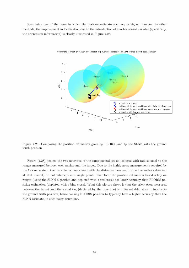
Examining one of the cases in which the position estimate accuracy is higher than for the othermethods, the improvement in localization due to the introduction of another sensed variable (specifically,the orientation information) is clearly illustrated in Figure 4.28.

Figure 4.28: Comparing the position estimation given by FLORIS and by the SLNN with the groundtruth position

Figure (4.28) depicts the two networks of the experimental set-up, spheres with radius equal to theranges measured between each anchor and the target. Due to the highly noisy measurements acquired bythe Cricket system, the five spheres (associated with the distances measured to the five anchors detectedat that instant) do not intercept in a single point. Therefore, the position estimation based solely onranges (using the SLNN algorithm and depicted with a red cross) has lower accuracy than FLORIS po-sition estimation (depicted with a blue cross). What this picture shows is that the orientation measuredbetween the target and the visual tag (depicted by the blue line) is quite reliable, since it interceptsthe ground truth position, hence causing FLORIS position to typically have a higher accuracy than theSLNN estimate, in such noisy situations.

62

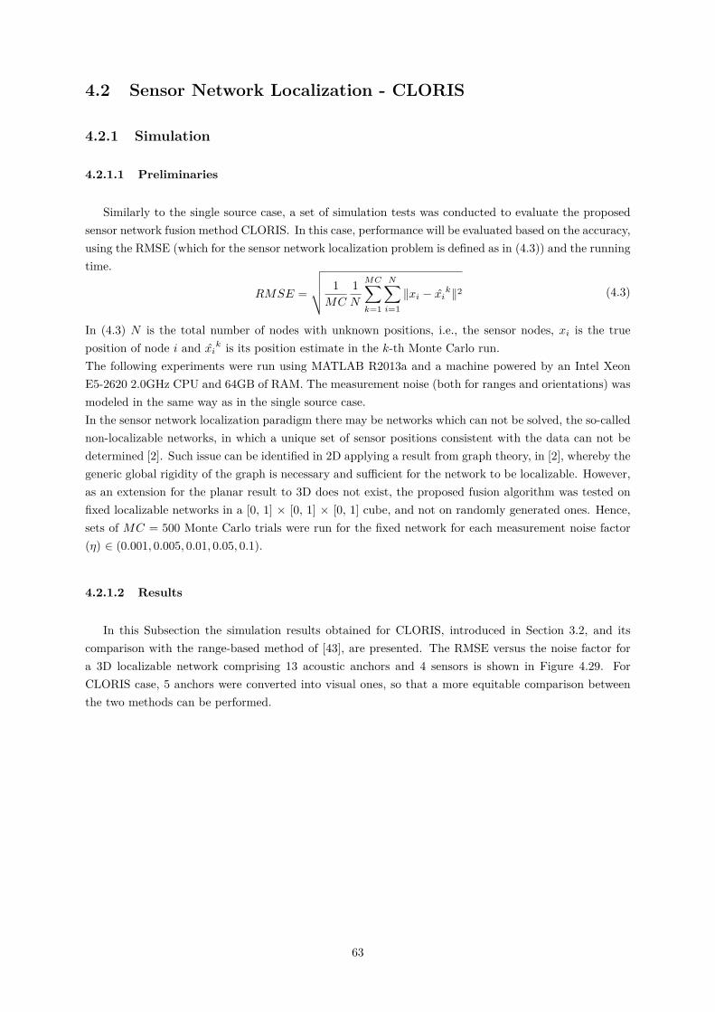
4.2 Sensor Network Localization - CLORIS

4.2.1 Simulation

4.2.1.1 Preliminaries

Similarly to the single source case, a set of simulation tests was conducted to evaluate the proposedsensor network fusion method CLORIS. In this case, performance will be evaluated based on the accuracy,using the RMSE (which for the sensor network localization problem is defined as in (4.3)) and the runningtime.

RMSE =

√√√√ 1MC

1N

MC∑k=1

N∑i=1‖xi − xik‖2 (4.3)

In (4.3) N is the total number of nodes with unknown positions, i.e., the sensor nodes, xi is the trueposition of node i and xi

k is its position estimate in the k-th Monte Carlo run.The following experiments were run using MATLAB R2013a and a machine powered by an Intel XeonE5-2620 2.0GHz CPU and 64GB of RAM. The measurement noise (both for ranges and orientations) wasmodeled in the same way as in the single source case.In the sensor network localization paradigm there may be networks which can not be solved, the so-callednon-localizable networks, in which a unique set of sensor positions consistent with the data can not bedetermined [2]. Such issue can be identified in 2D applying a result from graph theory, in [2], whereby thegeneric global rigidity of the graph is necessary and sufficient for the network to be localizable. However,as an extension for the planar result to 3D does not exist, the proposed fusion algorithm was tested onfixed localizable networks in a [0, 1] × [0, 1] × [0, 1] cube, and not on randomly generated ones. Hence,sets of MC = 500 Monte Carlo trials were run for the fixed network for each measurement noise factor(η) ∈ (0.001, 0.005, 0.01, 0.05, 0.1).

4.2.1.2 Results

In this Subsection the simulation results obtained for CLORIS, introduced in Section 3.2, and itscomparison with the range-based method of [43], are presented. The RMSE versus the noise factor fora 3D localizable network comprising 13 acoustic anchors and 4 sensors is shown in Figure 4.29. ForCLORIS case, 5 anchors were converted into visual ones, so that a more equitable comparison betweenthe two methods can be performed.

63

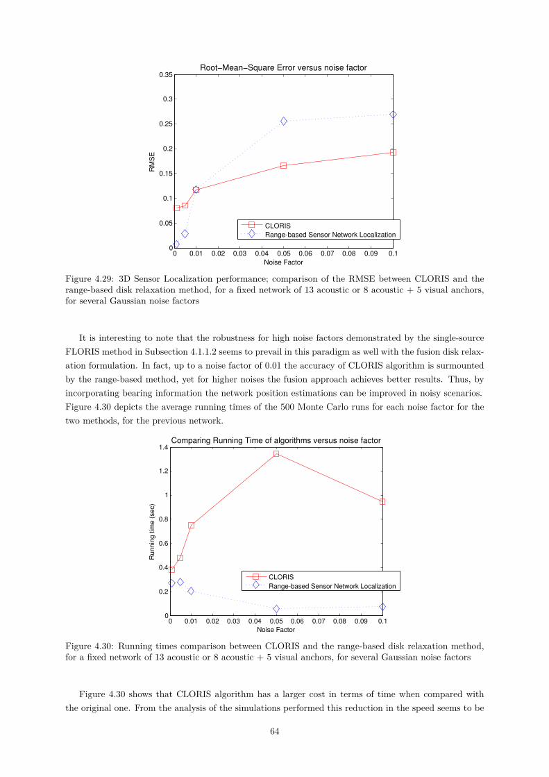
0 0.01 0.02 0.03 0.04 0.05 0.06 0.07 0.08 0.09 0.10

0.05

0.1

0.15

0.2

0.25

0.3

0.35

RM

SE

Noise Factor

Root−Mean−Square Error versus noise factor

CLORISRange-based Sensor Network Localization

Figure 4.29: 3D Sensor Localization performance; comparison of the RMSE between CLORIS and therange-based disk relaxation method, for a fixed network of 13 acoustic or 8 acoustic + 5 visual anchors,for several Gaussian noise factors

It is interesting to note that the robustness for high noise factors demonstrated by the single-sourceFLORIS method in Subsection 4.1.1.2 seems to prevail in this paradigm as well with the fusion disk relax-ation formulation. In fact, up to a noise factor of 0.01 the accuracy of CLORIS algorithm is surmountedby the range-based method, yet for higher noises the fusion approach achieves better results. Thus, byincorporating bearing information the network position estimations can be improved in noisy scenarios.Figure 4.30 depicts the average running times of the 500 Monte Carlo runs for each noise factor for thetwo methods, for the previous network.

0 0.01 0.02 0.03 0.04 0.05 0.06 0.07 0.08 0.09 0.10

0.2

0.4

0.6

0.8

1

1.2

1.4

Run

ning

time

(sec

)

Noise Factor

Comparing Running Time of algorithms versus noise factor

CLORISRange-based Sensor Network Localization

Figure 4.30: Running times comparison between CLORIS and the range-based disk relaxation method,for a fixed network of 13 acoustic or 8 acoustic + 5 visual anchors, for several Gaussian noise factors

Figure 4.30 shows that CLORIS algorithm has a larger cost in terms of time when compared withthe original one. From the analysis of the simulations performed this reduction in the speed seems to be

64

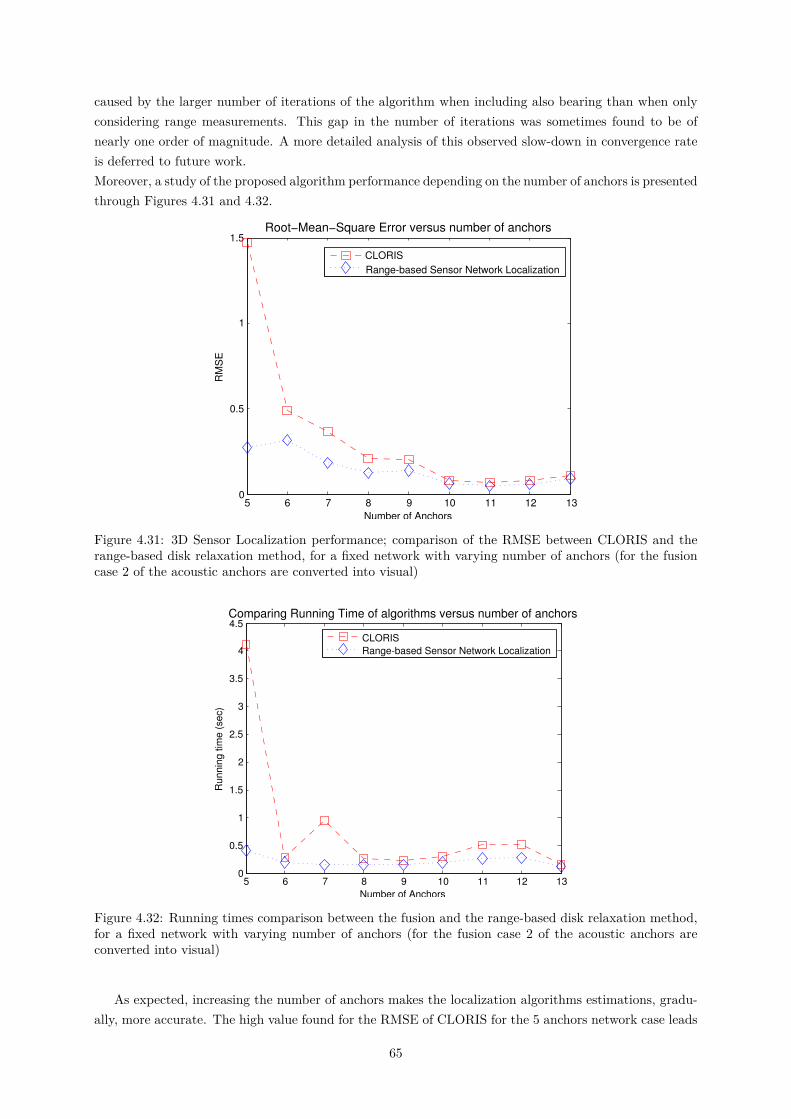
caused by the larger number of iterations of the algorithm when including also bearing than when onlyconsidering range measurements. This gap in the number of iterations was sometimes found to be ofnearly one order of magnitude. A more detailed analysis of this observed slow-down in convergence rateis deferred to future work.Moreover, a study of the proposed algorithm performance depending on the number of anchors is presentedthrough Figures 4.31 and 4.32.

5 6 7 8 9 10 11 12 130

0.5

1

1.5

RM

SE

Number of Anchors

Root−Mean−Square Error versus number of anchors

CLORISRange-based Sensor Network Localization

Figure 4.31: 3D Sensor Localization performance; comparison of the RMSE between CLORIS and therange-based disk relaxation method, for a fixed network with varying number of anchors (for the fusioncase 2 of the acoustic anchors are converted into visual)

5 6 7 8 9 10 11 12 130

0.5

1

1.5

2

2.5

3

3.5

4

4.5

Run

ning

time

(sec

)

Number of Anchors

Comparing Running Time of algorithms versus number of anchors

CLORISRange-based Sensor Network Localization

Figure 4.32: Running times comparison between the fusion and the range-based disk relaxation method,for a fixed network with varying number of anchors (for the fusion case 2 of the acoustic anchors areconverted into visual)

As expected, increasing the number of anchors makes the localization algorithms estimations, gradu-ally, more accurate. The high value found for the RMSE of CLORIS for the 5 anchors network case leads

65

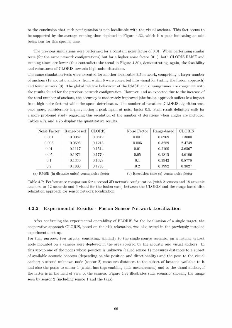
to the conclusion that such configuration is non localizable with the visual anchors. This fact seems tobe supported by the average running time depicted in Figure 4.32, which is a peak indicating an oddbehaviour for this specific case.

The previous simulations were performed for a constant noise factor of 0.01. When performing similartests (for the same network configurations) but for a higher noise factor (0.1), both CLORIS RMSE andrunning times are lower (this contradicts the trend in Figure 4.30), demonstrating, again, the feasibilityand robustness of CLORIS towards high noise situations.The same simulation tests were executed for another localizable 3D network, comprising a larger numberof anchors (18 acoustic anchors, from which 6 were converted into visual for testing the fusion approach)and fewer sensors (3). The global relative behaviour of the RMSE and running times are congruent withthe results found for the previous network configuration. However, and as expected due to the increase ofthe total number of anchors, the accuracy is moderately improved (the fusion approach suffers less impactfrom high noise factors) while the speed deteriorates. The number of iterations CLORIS algorithm was,once more, considerably higher, noting a peak again at noise factor 0.5. Such result definitely calls fora more profound study regarding this escalation of the number of iterations when angles are included.Tables 4.7a and 4.7b display the quantitative results.

Noise Factor Range-based CLORIS0.001 0.0082 0.08190.005 0.0695 0.12130.01 0.1117 0.15140.05 0.1976 0.17700.1 0.1330 0.13280.2 0.1800 0.1783

(a) RMSE (in distance units) versus noise factor

Noise Factor Range-based CLORIS0.001 0.6269 1.30000.005 0.3289 2.47490.01 0.2100 3.65670.05 0.1815 4.61060.1 0.3942 0.87780.2 0.1992 0.3027

(b) Execution time (s) versus noise factor

Table 4.7: Performance comparison for a second 3D network configuration (with 2 sensors and 18 acousticanchors, or 12 acoustic and 6 visual for the fusion case) between the CLORIS and the range-based diskrelaxation approach for sensor network localization

4.2.2 Experimental Results - Fusion Sensor Network Localization

After confirming the experimental operability of FLORIS for the localization of a single target, thecooperative approach CLORIS, based on the disk relaxation, was also tested in the previously installedexperimental set-up.For that purpose, two targets, consisting, similarly to the single source scenario, on a listener cricketnode mounted on a camera were deployed in the area covered by the acoustic and visual anchors. Inthis set-up one of the nodes whose position is unknown (called sensor 1) measures distances to a subsetof available acoustic beacons (depending on the position and directionality) and the pose to the visualanchor; a second unknown node (sensor 2) measures distances to the subset of beacons available to itand also the poses to sensor 1 (which has tags enabling such measurement) and to the visual anchor, ifthe latter is in the field of view of the camera. Figure 4.33 illustrates such scenario, showing the imageseen by sensor 2 (including sensor 1 and the tags).

66

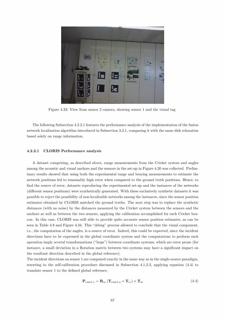
Figure 4.33: View from sensor 2 camera, showing sensor 1 and the visual tag

The following Subsection 4.2.2.1 features the performance analysis of the implementation of the fusionnetwork localization algorithm introduced in Subsection 3.2.1, comparing it with the same disk relaxationbased solely on range information.

4.2.2.1 CLORIS Performance analysis

A dataset comprising, as described above, range measurements from the Cricket system and anglesamong the acoustic and visual anchors and the sensors in the set-up in Figure 4.20 was collected. Prelim-inary results showed that using both the experimental range and bearing measurements to estimate thenetwork positions led to reasonably high error when compared to the ground truth positions. Hence, tofind the source of error, datasets reproducing the experimental set-up and the instances of the networks(different sensor positions) were synthetically generated. With these exclusively synthetic datasets it waspossible to reject the possibility of non-localizable networks among the instances, since the sensor positionestimates obtained by CLORIS matched the ground truths. The next step was to replace the syntheticdistances (with no noise) by the distances measured by the Cricket system between the sensors and theanchors as well as between the two sensors, applying the calibration accomplished for each Cricket bea-con. In this case, CLORIS was still able to provide quite accurate sensor position estimates, as can beseen in Table 4.8 and Figure 4.34. This “debug” process allowed to conclude that the visual component,i.e., the computation of the angles, is a source of error. Indeed, this could be expected, since the incidentdirections have to be expressed in the global coordinate system and the computations to perform suchoperation imply several transformations (“hops”) between coordinate systems, which are error prone (forinstance, a small deviation in a Rotation matrix between two systems may have a significant impact onthe resultant direction described in the global reference).The incident directions on sensor 1 are computed exactly in the same way as in the single-source paradigm,resorting to the self-calibration procedure discussed in Subsection 4.1.2.3, applying equation (4.4) totranslate sensor 1 to the defined global reference.

Pcam1 c = Rac (Tcam1 a + Tcc) + Tac (4.4)

67

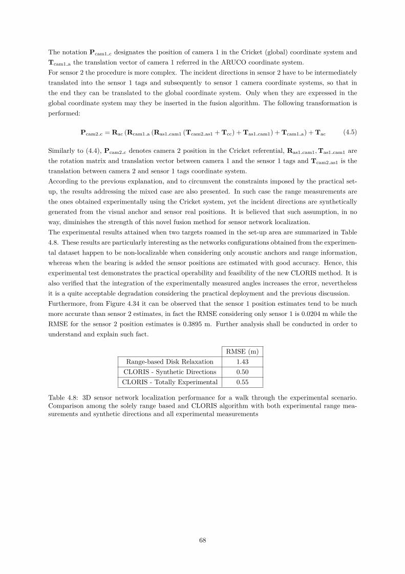
The notation Pcam1 c designates the position of camera 1 in the Cricket (global) coordinate system andTcam1 a the translation vector of camera 1 referred in the ARUCO coordinate system.For sensor 2 the procedure is more complex. The incident directions in sensor 2 have to be intermediatelytranslated into the sensor 1 tags and subsequently to sensor 1 camera coordinate systems, so that inthe end they can be translated to the global coordinate system. Only when they are expressed in theglobal coordinate system may they be inserted in the fusion algorithm. The following transformation isperformed:

Pcam2 c = Rac (Rcam1 a (Ras1 cam1 (Tcam2 as1 + Tcc) + Tas1 cam1) + Tcam1 a) + Tac (4.5)

Similarly to (4.4), Pcam2 c denotes camera 2 position in the Cricket referential, Ras1 cam1,Tas1 cam1 arethe rotation matrix and translation vector between camera 1 and the sensor 1 tags and Tcam2 as1 is thetranslation between camera 2 and sensor 1 tags coordinate system.According to the previous explanation, and to circumvent the constraints imposed by the practical set-up, the results addressing the mixed case are also presented. In such case the range measurements arethe ones obtained experimentally using the Cricket system, yet the incident directions are syntheticallygenerated from the visual anchor and sensor real positions. It is believed that such assumption, in noway, diminishes the strength of this novel fusion method for sensor network localization.The experimental results attained when two targets roamed in the set-up area are summarized in Table4.8. These results are particularly interesting as the networks configurations obtained from the experimen-tal dataset happen to be non-localizable when considering only acoustic anchors and range information,whereas when the bearing is added the sensor positions are estimated with good accuracy. Hence, thisexperimental test demonstrates the practical operability and feasibility of the new CLORIS method. It isalso verified that the integration of the experimentally measured angles increases the error, neverthelessit is a quite acceptable degradation considering the practical deployment and the previous discussion.Furthermore, from Figure 4.34 it can be observed that the sensor 1 position estimates tend to be muchmore accurate than sensor 2 estimates, in fact the RMSE considering only sensor 1 is 0.0204 m while theRMSE for the sensor 2 position estimates is 0.3895 m. Further analysis shall be conducted in order tounderstand and explain such fact.

RMSE (m)Range-based Disk Relaxation 1.43

CLORIS - Synthetic Directions 0.50CLORIS - Totally Experimental 0.55

Table 4.8: 3D sensor network localization performance for a walk through the experimental scenario.Comparison among the solely range based and CLORIS algorithm with both experimental range mea-surements and synthetic directions and all experimental measurements

68

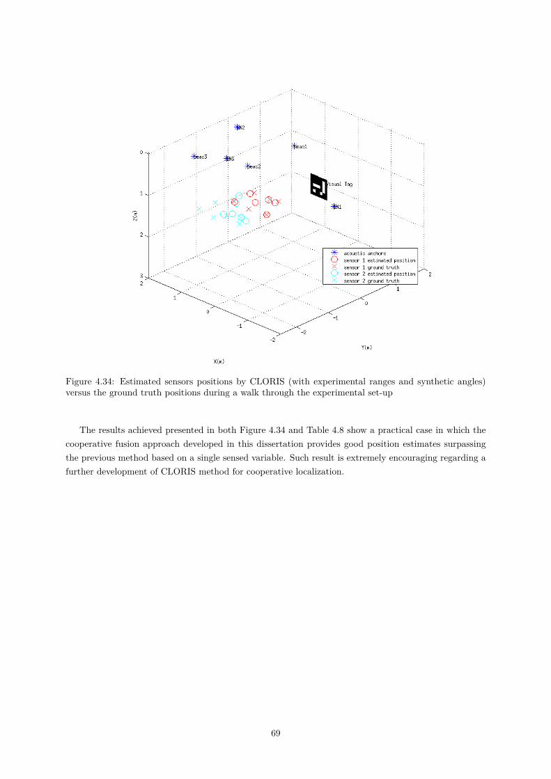
Figure 4.34: Estimated sensors positions by CLORIS (with experimental ranges and synthetic angles)versus the ground truth positions during a walk through the experimental set-up

The results achieved presented in both Figure 4.34 and Table 4.8 show a practical case in which thecooperative fusion approach developed in this dissertation provides good position estimates surpassingthe previous method based on a single sensed variable. Such result is extremely encouraging regarding afurther development of CLORIS method for cooperative localization.

69

Chapter 5

Conclusions

This Chapter presents the major contributions and attained results of this dissertation (in Section5.1) and discusses, in further detail, some foreseen directions for future research on this topic (in Section5.2).

5.1 Achievements

The work presented in this dissertation successfully addressed the growing need for solutions and ap-plications for large scale heterogeneous sensor networks, taking advantage of the distinct sensing devices.More precisely, this work provides accurate indoor localization methods that can use different types ofproximity information, namely ranges and incident directions estimated from video images, in a totallyintegrated fashion.A new formulation based on a nonconvex LS joint formulation fusing information from ranges and an-gles and a tight convex relaxation for this problem were devised. The single-source method was calledFLORIS, owing to the geometry of the formulation.Additionally, a procedure to derive the observation model and its parameters - a key component for in-formation fusion that expresses spatial data acquired from the two separate sensor networks in a commonreference frame - is proposed. This calibration procedure was analytically and experimentally testedenabling integration of the localization system in the deployed experimental set-up.In the same vein, this dissertation also targeted the collaborative scenario (i.e., the sensor network local-ization problem) for heterogeneous measurements. The proposed CLORIS algorithm is an extension ofa previous sensor network localization method developed in-house and based on a convexification mech-anism by disk relaxation.The results obtained show that the both methods can provide accurate localization. More quantitatively,FLORIS method achieves, in numerical results, lower RMSE (thus higher accuracy) than state-of-the-artrange-only methods, specially for high noise scenarios, while the running times are comparable with theformer preferred method (SLNN). In this way it can be claimed that the newly proposed FLORIS has asimilar performance or even outperforms, in some cases, the previous existing localization methods.Simulation results for the collaborative scenario were extremely promising too. Again, the algorithm’smost salient feature is high accuracy in the presence of strong observation noise, thus presenting a goodperformance trade-off when compared to the range-only methods.Moreover, an experimental set-up was deployed leading to a validation of the feasibility and robustness of

71

the algorithms in real application scenarios for the two localization paradigms. Although several physicalsetbacks were found, most of them were surpassed, allowing for an entirely integrated implementationof FLORIS and CLORIS. Both methods showed very good behaviour in the real scenario, with betteraccuracy than benchmark algorithms in the conducted tests. The experimental findings clearly motivatefurther implementations, using higher performance technologies and devices.

5.2 Future Work

As multiple future work directions were identified during this dissertation work, this Section is dividedinto topics, detailing, for each, the further improvements foreseen.

5.2.1 Range

The variables sensed to obtain distance information for the proposed hybrid localization method are animportant practical concern, thus alternative technologies to acoustic based sensors, such as the Cricketsystem which was shown to provide noisy range measurements, shall be addressed.Received Signal Strength Indication (RSSI) is one technique that measures pseudo-ranges (since the rangeis computed using a function that relates the power magnitude with distance) and that can be advan-tageous. In fact, although the resulting range measurements can be quite noisy, they can be obtainedusing low complexity hardware and in an inexpensive way. Furthermore, this technology can providelarge datasets, which can be most convenient to an EDM approach (discussed in 5.2.4), in which thelocalization problem is formulated as an EDM completion.Another technology that should be taken into account is Wi-Fi, mainly due to its ubiquitousness in theenvisaged practical application scenarios. As the majority of smart devices have Wi-Fi receptors, an hy-brid system relying on such technology to obtain the distance measurements would be easy to implementwith widespread acceptance.Lastly, in challenging environments such as indoors, owing to interferences, occlusions and multi-path, [45]suggests ultra-wideband (UWB) transmission technology, albeit being currently expensive, as a promisingalternative for localization. Thus, exploring (low-cost) UWB nodes is another future prospect.

5.2.2 Vision

The method developed in this work can be seen, regarding the vision component, as a first step/phaseto the exploration of objects/patterns present in the environment. Effectively, an evolution from theuse of (augmented reality) markers/tags as visual anchors to general known objects spread throughoutthe surroundings is a natural evolution for this work. Thus, object/pattern detection and recognitionalgorithms should be applied in order to obtain the bearing from visual anchors. This final phase wouldresort to the Bag of Words image representation and use methods such as SIFT (Scale-Invariant FeatureTransform) [27], following the work developed by Lampert et al. [25], which allows the use of classifiersfor object localization that were previously considered too slow for this task, since the convergence to theglobal solution is in sub-linear time.

72

5.2.3 Cooperative paradigm

In regard to the sensor network localization problem, although the attained results both in simulationand experimentally were positive, there is still room for improvement. Namely, one of the identifiedissues concerns the large number of iterations executed by the disk relaxation algorithm when angles areconsidered, which degrades the retrieved running times. Thus, a deeper analysis of the computationsassociated with the incident directions and their projections onto lines, performed during Nesterov’sgradient descent method, is pertinent.Furthermore, a potential formulation with fine tuned weights for the range and angular components shallbe assessed. Effectively, exploratory tests suggest that varying the weights assigned to the heterogeneousmeasurements, rather than considering an equal influence in the cost function, may have a positive impactin the obtained results.Another aspect that was proven to have impact in the experimental localization performance is theprocedure to translate between the coordinate systems for the various types of nodes. Certainly thishas also impact in the single-source localization paradigm, yet it has more negative consequences inthe cooperative case since more poses from the multiple sensors must be expressed, via the knowntransformations, in the global referential system. A robust method to execute such transformation to acommon coordinate system shall be devised, as such procedure has high sensitivity to small fluctuationsof the entries of rotation matrices. Additionally, a flawless calibration of the cameras is mandatory forany devised procedure. In fact, the general underperformance found for the experimental results shouldbe partly consequence of physical limitations and constraints of the available hardware.

5.2.4 Exploring other constraints

Parallel to the line of work followed in this dissertation, based on ML/LS approaches, an innovativeapproach exploring the low rank properties of EDM is foreseen. With the ranges available, the distanceestimation should be formulated as an EDM completion problem, as found in the literature [32, 31, 23].Furthermore, the completion problem will use the rank constraint, as the matrix rank is given by thesubspace where localization is being performed (most commonly 3D). A matrix (D) comprising all theEDM (per column, using the vectorization operation) related to each instant of the target trajectorywill be built and a decomposition in a matrix with the correct “clean” distances (Dr) added with theerror (E) is pursued. A formulation consisting in a cost function with both matrices, penalizing theerror matrix and a low rank constraint imposed to the “clean” matrix will be sought. To obtain suchdecomposition from a matrix built from batches of measurements, dealing with the outliers, a techniquecalled Sparse Subspace Clustering (SSC) [17] could be applied. This method [17] proposes a convexrelaxation to represent data points from a high-dimensional space as a sparse linear affine combinationof the remaining points from a low-dimensional subspace.Also, a more theoretical approach may be explored regarding the use of the rank constraint in the EDMcompletion problem. In this topic the rank evolution in several EDMs formed by the moving target in awireless network for each time instant will be studied. With this secondary approach we will try to devisea new formulation for the problem of localizing and tracking a single moving source (not addressed inthis Thesis). In this scenario a dependence of the position estimation on prior estimates combined withthe target trajectory information may be established.Under this EDM completion approach the case in which not all distances between the sensors and anchorsare available, i.e., the missing data case, is inherently addressed.Moreover, it should be stressed that promising cues regarding a unified fusion using EDMs have been

73

found. In fact, low rank constraints are used not only in WSN localization (via EDMs), as aforementioned,but also, more recently, in several traditional vision methods/problems [10]. Such fact paves the way tofurther research in this topic, strongly suggesting that a common methodology, integrating both rangesand orientations can be devised. This approach could be applied together with 3D reconstruction mapsas in [1].

74

References

[1] S. Agarwal, Y. Furukawa, N. Snavely, I. Simon, B. Curless, S. M. Seitz, and R. Szeliski. BuildingRome in a Day. Communications of the ACM, 54(10):105–112, Oct 2011.

[2] B. Anderson, I. Shames, G. Mao, and B. Fidan. Formal Theory of Noisy Sensor Network Localization.SIAM Journal on Discrete Mathematics, 24(2):684–698, Feb. 2010.

[3] J. Bachrach and C. Taylor. Localization in Sensor Networks, in Handbook of Sensor Networks:Algorithms and Architectures. John Wiley & Sons, 2005.

[4] J. P. Ballantine and A. R. Jerbert. Distance from a line, or plane, to a point. The AmericanMathematical Monthly, 59(4):242–243, Apr. 1952.

[5] A. Beck and P. Stoica. Exact and Approximate Solutions of Source Localization Problems. IEEETransactions on Signal Processing, 56(5):1770–1778, May 2008.

[6] P. Biswas. Semidefinite Programming Approaches to Distance Geometry Problems. PhD thesis,Stanford University, 2007.

[7] P. Biswas, H. Aghajan, and Y. Ye. Integration of Angle of Arrival Information for Multimodal SensorNetwork Localization using Semidefinite Programming. In Proceedings of 39th Asilomar Conferenceon Signals, Systems and Computers, 2005.

[8] P. Biswas and Y. Ye. Semidefinite Programming for Ad Hoc Wireless Sensor Network Localization.In Proceedings of the third international symposium on Information processing in sensor networks,pages 45 – 54. ACM, 2004.

[9] S. Boyd and L. Vandenberghe. Convex Optimization. Cambridge University Press, 2004.

[10] R. S. Cabral, D. Fernando, J. P. Costeira, and A. Bernardino. Unifying Nuclear Norm and BilinearFactorization Approaches for Low-rank Matrix Decomposition. In IEEE International Conferenceon Computer Vision (ICCV), pages 2488 – 2495, 2013.

[11] R. S. Cabral, D. Fernando, J. P. Costeira, and A. Bernardino. Matrix Completion for Weakly-supervised Multi-label Image Classification. IEEE Transactions on Pattern Analysis and MachineIntelligence, in press, online July 2014.

[12] G. Calafiore, C. L., and M. Wei. Distributed optimization techniques for range localization innetworked systems. In Proceedings of the 49th IEEE Conference on Decision and Control (CDC),pages 2221–2226, 2010.

[13] K. Cheung, W. Ma, and H. So. Accurate approximation algorithm for TOA based maximum likeli-hood mobile location using semidefinite programming. In Proceedings of IEEE Int. Conf. Acoust.,Speech, Signal Process (ICASSP’04), pages 145–148, Montreal, Canada, 2004. IEEE.

[14] M. Crocco, A. D. Bue, I. B. Barbosa, and V. Murino. A Closed Form Solution for the Self-Calibrationof Heterogeneous Sensors. In Procedings of the British Machine Vision Conference 2012, Los Angeles,California, 2012.

[15] M. Crocco, A. D. Bue, and V. Murino. A Bilinear Approach to the Position Self-Calibration ofMultiple Sensors. IEEE Transactions on Signal Processing, 60(2):660–673, Feb. 2012.

75

[16] G. Destino and G. Abreu. On the maximum likelihood approach for source and network localization.IEEE Transactions on Signal Processing, 59(10):4954–4970, Oct. 2011.

[17] E. Elhamifar and R. Vidal. Sparse Subspace Clustering. In IEEE Conference on Computer Visionand Pattern Recognition, 2009. CVPR 2009, pages 2790 – 2797. IEEE, 2009.

[18] F. Endres, J. Hess, N. Engelhard, J. Sturm, D. Cremers, and W. Burgard. An Evaluation of theRGB-D SLAM System. In Procedings of the 2012 IEEE International Conference on Robotics andAutomation, pages 1691 – 1696, 2012.

[19] M. Fischler and R. Bolles. Random Sample Consensus: A Paradigm for Model Fitting with Applica-tions to Image Analysis and Automated Cartography. Communications of the ACM, 24(6):381–395,June 1981.

[20] S. Funiak, C. Guestrin, M. Paskin, and R. Sukthankar. Distributed Localization of NetworkedCameras. In 5th International Conference on Information Processing in Sensor Networks, pages34–42, 2006.

[21] S. Garrido-Jurado, R. Munoz-Salinas, F. J. Madrid-Cuevas, and M. J. MarıÂŋn-Jimenez. Automaticgeneration and detection of highly reliable fiducial markers under occlusion. Pattern Recognition,47(6):2280 – 2292, 2014.

[22] M. Gholami, L. Tetruashvili, E. Strom, and Y. Censor. Cooperative Wireless Sensor Network Posi-tioning via Implicit Convex Feasibility. Signal Processing, IEEE Transactions on, 61(23):5830–5840,Dec 2013.

[23] J. Gomes, E. Zamanizadeh, J. Bioucas-Dias, J. Alves, and T. C. Furfaro. Building location awarenessinto acoustic communication links and networks through channel delay estimation Categories andSubject Descriptors. In WUWNet’12 7th ACM International Conference on Underwater Networks& Systems, Los Angeles, California, 2012.

[24] N. Krislock and H. Wolkowicz. Handbook on Semidefinite, Conic and Polynomial Optimization.Springer, 2012.

[25] C. H. Lampert, M. Blaschko, and T. Hofmann. Beyond sliding windows: Object localization byefficient subwindow search. In IEEE Conference on Computer Vision and Pattern Recognition,2008. CVPR 2008, pages 1–8. IEEE, 2008.

[26] L. Liberti, C. Lavor, N. Maculan, and A. Mucherino. Euclidean distance geometry and applications.arXiv:1205.0349v1, 2012.

[27] D. Lowe. Object recognition from local scale-invariant features. In Proceedings of the Seventh IEEEInternational Conference on Computer Vision, 1999 (Volume:2), pages 1150–1157. IEEE, 1999.

[28] M. Marques and J. P. Costeira. Estimating 3D shape from degenerate sequences with missing data.Computer Vision and Image Understanding, 13(2):261–272, Feb. 2011.

[29] A. Mulloni, D. Wagner, I. Barakonyi, and D. Schmalstieg. Indoor Positioning and Navigation withCamera Phones. IEEE Pervasive Computing, 8(2):2–31, Apr. 2009.

[30] Y. Nesterov. A method of solving a convex programming problem with convergence rate o (1/k2).Soviet Mathematics Doklady, 27(2):372–376, Feb. 1983.

[31] P. Oguz-Ekim, J. Gomes, and P. Oliveira. RSS Based Cooperative Sensor Network Localization withUnknown Transmit Power. In Proceedings of Signal Processing and Communications ApplicationsConference (SIU), 2013 21st, pages 1–4. IEEE, 2013.

[32] P. Oguz-Ekim, J. Gomes, J. Xavier, and P. Oliveira. Robust Localization of Nodes and Time-Recursive Tracking in Sensor Networks Using Noisy Range. IEEE Transactions on Signal Processing,59(8):3930–3942, Aug. 2011.

[33] P. Oguz-Ekim, J. Gomes, J. Xavier, M. Stosic, and P. Oliveira. Approximate Maximum LikelihoodSource Localization from Range Measurements Through Convex Relaxation. arXiv:1111.6755v1,2011.

76

[34] P. Oguz-Ekim, J. Gomes, J. Xavier, M. Stosic, and P. Oliveira. An Angular Approach for Range-Based Approximate Maximum Likelihood Source Localization Through Convex Relaxation. IEEETransactions on Wireless Communications, 13(7):3951–3964, July 2014.

[35] N. Patwari, J. Ash, S. Kyperountas, A. Hero, R. Moses, and N. Correal. Locating the nodes:cooperative localization in wireless sensor networks. Signal Processing Magazine, IEEE, 22(4):54–69, July 2005.

[36] N. B. Priyantha, A. Chakraborty, and H. Balakrishnan. The Cricket Location-Support System. InThe Proceedings of the sixth ACM International Conference on Mobile Computing and Networking(ACM Mobicom 2000), pages 32–43, 2000.

[37] A. Rahimi, B. Dunagan, and T. Darrell. Simultaneous Calibration and Tracking with a Networkof Non-Overlapping Sensors. In Proceedings of the 2004 IEEE Computer Society Conference onComputer Vision and Pattern Recognition, 2004, pages 187–194. IEEE, 2004.

[38] P. F. R. C. Santos. Mapeamento e Localizacao em Forma Fechada. Master’s thesis, Instituto SuperiorTecnico, 2013.

[39] D. Schneider. You Are Here. IEEE Spectrum, 50(12):34–39, Dec. 2013.

[40] Y. Shang, W. Rumi, Y. Zhang, and F. M. Localization from connectivity in sensor networks. IEEETransactions on Parallel and Distributed Systems, 15(11):961–974, Nov. 2004.

[41] Q. Shi, C. He, H. Chen, and L. Jiang. Distributed wireless sensor network localization via sequentialgreedy optimization algorithm. IEEE Transactions on Signal Processing, 58(6):3328–3340, June2010.

[42] A. Simonetto and G. Leus. Distributed maximum likelihood sensor network localization. IEEETransactions on Signal Processing, 62(6):1424–1437, Mar. 2014.

[43] C. Soares, J. Xavier, and J. Gomes. Simple and fast cooperative localization for sensor networks.arXiv:1408.4728v1 [math.OC], 2014.

[44] S. Wang and H. Hu. Wireless Sensor Networks for Underwater Localization: A Survey. TechnicalReport CES-521, School of Computer Science and Electronic Engineering University of Essex, UnitedKingdom, May 2012.

[45] H. Wymeersch, J. Lien, and M. Win. Cooperative Localization in Wireless Networks. Proceedingsof the IEEE, 97(2):427–450, Feb. 2009.

77