HYBRID ELECTRIC VEHICLE OWNERSHIP AND FUEL ECONOMY ACROSS

TEXAS: AN APPLICATION OF SPATIAL MODELS

Prateek Bansal

Graduate Research Assistant

Department of Civil, Architectural and Environmental Engineering

The University of Texas at Austin

prateekbansal@utexas.edu

Kara M. Kockelman

(Corresponding author)

E.P. Schoch Professor in Engineering

Department of Civil, Architectural and Environmental Engineering

The University of Texas at Austin

kkockelm@mail.utexas.edu

Phone: 512-471-0210

Yiyi Wang

Assistant Professor

Montana State University

Civil Engineering Department

yiyi.wang@ce.montana.edu

The following paper is a pre-print, the fnal publication can be found in the Transportation Research Record No. 2495: 53-64, 2015.

ABSTRACT

Policymakers, transport planners, automobile manufacturers, and others are interested in the

factors that affect adoption rates of electric vehicles and more fuel efficient vehicles. Using

Census-tract-level data and registered vehicle counts across Texas counties in 2010, this study

investigated the impact of various built environment and demographic attributes, including land

use balance, employment density, population densities, median age, gender, race, education,

household size, and income. To allow for spatial autocorrelation (across census tracts) in

unobserved components of vehicle counts by tract, as well as cross-response correlation (both

spatial and local/aspatial in nature), models of ownership levels (vehicle counts, by vehicle type

and fuel economy level) were estimated using bivariate and trivariate Poisson-lognormal

conditional autoregressive models. The presence of high spatial autocorrelations and local cross-

response correlations is consistent in all models, across all counties studied. Fuel-efficient-

vehicle ownership rates were found to rise with household incomes, resident education levels,

and the share of male residents, and fall in the presence of larger household sizes and higher jobs

densities.

The average fuel economy of each tract’s light-duty vehicles were also analyzed, using a spatial

error model, across all Texas tracts; and this variable was found to depend most on educational

attainment levels, median age, income, and household size variables, though all covariates used

were statistically significant. If households registering more fuel-efficient vehicles, including

hybrid EVs, are also more inclined to purchase plug-in EVs, these findings can assist in spatial

planning of charging infrastructure as well as other calculations (such as gas-tax revenue

implications).

Key Words: electric vehicles, fuel economy, vehicle ownership, spatial econometric models

INTRODUCTION

Many worry about the world’s continuing reliance on petroleum as a transportation fuel, with

various air quality impacts and energy security issues. Fuel economy is a salient feature of

automobiles, and fuel-efficient hybrid electric vehicles (HEVs) are achieving some marketplace

success (Keith 2012, Chen et al. 2014, Paul et al. 2011, Dijk et al. 2013). For example, 495,000

HEVs were sold in the United States in 2013, with over 1.5 million sold worldwide (EVs Roll

2014). Only 96,000 plug-in EVs (PEVs) were sold in the US in 2013, which includes 47,700

battery-only EVs (EVs Roll 2014), so the PEV future is less certain. Since market success

depends on consumer response, understanding the factors that affect purchase and use of more

fuel efficient and electric vehicles becomes crucial for sales and use forecasts, as well as energy

and environmental policies (Koo et al. 2012).

While EV sales (including both HEVs and PEVs) have risen considerably in the United

States over the past decade, high adoption rates tend to concentrate in a relatively few cities and

neighborhoods. In the case of Texas, Figure 1 shows how HEV ownership rates (per 1,000

registered light-duty vehicles [LDVs]) concentrate in the state’s biggest cities/regions: San

Antonio, Austin, Dallas-Ft. Worth, and Houston. (Since almost no PEVs were registered in

Texas in year 2010 [according to the vehicle decoder used on the DMV database], only HEV

counts were non-negligible in the 2010 Texas data sets, and thus analyzed separately from

conventional vehicles here.) Within these regions, spatial variation is striking (Figure 1).

Understanding of the factors behind such variations provides direction for policymaking,

planning, production, and marketing.

One reason for the clustering in HEV ownership rates is presumably spatial correlation in

local government incentives and marketing, demographics, and land use patterns (Kodjak 2012,

Chen et al. 2014). Another reason for the clustering relates to the theory of social contagion, with

consumers more likely to buy EVs if they see them regularly, on nearby roads, in neighbor’s

driveways, and being driven by their friends and colleagues (Axsen and Kurani 2011). Positive

contagion feedbacks can intensify to create adoption inhomogeneity at different scales.

This study’s first two models employ a multivariate conditional autoregressive (MCAR)

specification (as developed by Wang and Kockelman [2013] and applied in Chen et al. [2014]) to

understand many of the factors responsible for adoption rates of HEVs and other classes (based

on fuel economy) of LDVs across Texas’ major cities, while recognizing correlations that

emerge over space across vehicle ownership types. The paper’s bivariate model (Model 1)

estimates counts of HEVs vs. non-HEV passenger vehicles in each of the four largest counties of

Texas’ top 4 regions. The trivariate model (Model 2) examines tract-level registration numbers in

each of 3 fuel-economy-based vehicle classes (fuel efficient [>25 mi/gal], regular [15 to 25

mi/gal], and fuel inefficient [ 15 mi/gal]). A third model (Model 3) is of average fuel economy,

across all census tracts of Texas, and so relies on a continuous-response spatial error model for

spatial autocorrelation (Wall 2004, Kissling et al. 2008, and Anselin 1988).

FIGURE 1. HEV Adoption Rates in Year 2010 HEV counts per 10,000 light-duty vehicles

across Texas Census Tracts (using Texas Department of Motor Vehicles registration data, 2010)

BACKGROUND AND LITERATURE REVIEW

Several researchers have developed choice models to identify key factors encouraging EV and

other vehicle purchases. For example, Li et al. (2013) used a bivariate probit model to find that

consumers with environmentally-relevant information (from the Internet or friends) were more

likely to purchase HEVsthan flex-fuel vehicles, whereas males, those driving more miles, and

those registered as Republicans were less inclined. He et al.’s (2012) hierarchical choice model

analysis of the U.S. National Household Travel Survey (NHTS) 2009 and Vehicle Quality

Survey data found that those primarily making local trips (versus highway-based trips) and those

with higher education have a more positive attitude toward buying an HEV. Caulfield’s (2010)

survey of an Irish car company’s new customers suggest that preferences depend significantly on

vehicle price, reliability, safety, and fuel costs. Liu (2014) estimated that U.S. consumers are

willing to pay, on average, from $960 to $1720 more (depending on their income category) for

HEVs, which is lower than an HEV’s typical price premium. Jenn et al. (2013) estimated that the

Energy Policy Act of 2005 caused a 4.6% increase in U.S. HEV sales for every $1000 incentive

provided (per HEV). Liu (2014) concluded that offering $1000 and $3000 tax savings would

increase U.S. HEV sales by 4% and over 13% respectively. Using a 5% discount rate, Tuttle and

Kockelman (2012) estimated that gas prices above approximately $5.90, $5.00, and $3.75 per

gallon are estimated to make the Leaf, Volt, and Prius-PHEV (as offered in year 2011) more

financially attractive, respectively, than their conventional counterparts - without any credits. In

Musti and Kockelman’s (2011) survey, 76% of Austinites (with sample weighted to reflect true

local population) stated that fuel economy lies in their top three criteria for vehicle purchase, and

56% claimed they would consider purchasing a plug-in HEV if it were to cost $6,000 more than

its internal combustion counterpart (vs. just 36% of all U.S. respondents in Paul et al.’s [2011]

follow-up survey).

Very few studies have explored spatial variations and neighborhood effects in HEV

adoption rates. Keith et al. (2012) developed a spatial diffusion model to understand the reasons

behind high-adoption clusters of the Toyota Prius HEV across the United States. For greatest

impact or sales increases, they concluded that HEV adoption should be incentivized in regions

already exhibiting strong adoption. Chen et al. (2014) employed an MCAR model to anticipate

LDV registration counts of the Prius HEV, other EVs, and conventional (internal combustion)

vehicles across 1000 census block groups in the city of Philadelphia. They found that more

central/core zones and those with more higher-income households have higher EV ownership

rates, and that spatial correlations exist in unobserved terms (not controlled for by their set of

eleven covariates).

Auto purchases by individuals are arguably not as rational as those by fleet managers,

who have the time and expertise to do rigorous net present valuations. To understand Americans’

willingness to pay for fuel savings, Greene et al. (2013) surveyed 1000 US households four

times: in 2004, 2011, 2012 and 2013. Each time, they estimated that US car buyers expect fuel

economy savings to payback up-front vehicle costs in just 3 years, suggesting consumer myopia,

significant risk aversion (to car loss, rather than gas price increases), and/or a very high personal

discount rate (on a vehicle’s future benefits). They argue that accuracy of fuel economy

information is extremely important, because its uncertainty leads loss-averse consumers to

significantly undervalue fuel savings. In some contrast, Koo et al. (2012) calibrated mixed logit

and mixed multiple discrete continuous extreme value (MDCEV) models for Koreans’ recent

vehicle purchases, and concluded that Koreans tend to care most about fuel economy. Axsen and

Kurani (2013) found that new-vehicle buyers in California prefer HEVs and PEVs, not only

because of their functional benefits (e.g., lowered gasoline use and emissions), but also due to

their image association (with intelligence, responsibility, and support for the environment and

national energy security).

As noted above, most studies on vehicle choice are disaggregated in nature. Few studies

have explored spatial variations in adoption rates or have worked with complete samples. This

study employs rigorous and behaviorally plausible spatial models to better illuminate overall

factors that affect fuel economy choices and adoption rates of HEVs and other LDVs across

much of the U.S.’s second largest state.

DATA DESCRIPTION

This study uses the Texas Department of Motor Vehicles’ (DMV’s) vehicle registration counts

for year 2010. This database includes all registered vehicles in Texas, from cement trucks and

combines harvesters to passenger cars and motorized scooters. The fuel type and fuel economy

of vehicles were added to the DMV data using a vehicle identification number (VIN) decoder, as

purchased by Texas A&M University’s Dr. Steve Puller, and able to decode all vehicles with

model years newer than 1980. To provide anonymity to households, the final data set shows only

total vehicle counts by fuel type (hybrid, diesel, flex fuel, and gasoline) and fuel economy (miles

per gallon, MI/GAL) across Texas census tracts.

Out of the state’s 22.81 million registered-vehicle records, the LDV decoder was able to

match 17.35M vehicles to fuel information, leaving 5.19 million unmatched due to an early

model year (before 1981) or commercial-vehicle status (heavy- and medium-duty trucks and

agricultural equipment that sometimes runs on roadways. The VIN decoder also placed all plug-

in HEVs and battery EVs in the “unknown” category. For another 205,630 vehicle records

(0.90% of the database), fuel type was identified but not census tract, and for another 63,296

vehicle records (0.28% of registered vehicles), neither tract nor fuel information was matched.

Puller’s team coded the 2010 vehicles to the U.S. census tract system of year 2000 (in

order to map to census income data). For consistency in covariate timing, the count data were

transferred to the year 2010’s system using a census tract relationship file (US Census Bureau

2010). Texas’ tract counts in years 2000 and 2010 were 4388 and 5265, respectively; so 2010

tracts are somewhat smaller, reflecting a higher year 2010 state population (25.1M in 2010

versus 20.8M in 2000). 2200 of the year-2000 census tracts remained intact, while the rest split

or merged. Vehicle counts in modified tracts come from a population-weighted average of year-

2000 person counts.

This study relies on three models of vehicle type and fuel economy. The first two are

multivariate models for vehicle counts by type: Model 1 is a bivariate model with HEV and non-

HEV counts (in each census tract) as the response variables. Model 2 is a trivariate model with

vehicle counts in three fuel economy bins as the response variables. Model 2’s three fuel

economy levels are determined by thresholds one standard deviation (4.81 mi/gal) away from the

mean fuel economy (19.30 mi/gal) for the state’s entire LDV fleet. After rounding those

thresholds, the bins’ cut points are 15 mi/gal and 25 mi/gal. The vehicles falling into these low,

medium and high fuel economy categories are referred to here as “fuel inefficient”, “regular”

(fuel economy), and “fuel efficient” vehicles, respectively. Finally, Model 3 relies on a single,

continuous response variable, average fuel economy per tract, along with a spatial error model

(Cressie 1993 and Anselin 1988). Figure 2 shows a histogram of fuel economy across Texas’s

LDV fleet, as registered in the year 2010.

The model’s covariates mainly capture census-tract-level demographic attributes, like

average age, gender, race, household size, education, population density, number of commuting

workers, and income. These tract-level covariates come from the U.S. Census of Population

2010 database (which offers a complete sample of many variables) and the 2010 American

Community Survey (ACS) estimates (which samples a share of households every year, for a host

of additional variables). 5,188 Census tracts (out of Texas’s 5,265 tracts) offered complete data

for the aforementioned covariates and response variables. Jobs density and land use balance1

variables were also obtained for Travis County from the Capital Area Metropolitan Planning

Organization. Table 1 provides summary statistics of all census tract level variables. Since

vehicle counts should (in theory) scale with population counts (e.g., one may expect a doubling

in vehicle registrations when tract population is doubled), tract population variable is used an

exposure variable for the count models. Due to this scaling, many covariates are controlled for as

fractions, rather than as counts.

1 Land use balance was computed using the following entropy term (from Cervero and Kockelman [1997]):

(∑ ) ( )⁄ , where is the proportion of land use type k (including residential, commercial, office,

and industry uses) in the tract. An equal or uniform balance (with 25% of land falling into each of the four

categories) yields the maximum entropy value of 1.

FIGURE 2. Histogram of Fuel Economy across All Registered Light-duty Vehicles in Texas

(2010)

TABLE 1. Summary Statistics of Model Variables at Census Tract Level across Texas (2010) Variable Name Mean Median Std. Dev. Min Max

Dependent Variables

Vehicle Count (# LDVs per tract) 3,336 2,968 2,134 74 51,399

Model 1

# Hybrid EVs in tract 16.56 9.50 21.88 0 500

# Non-Hybrid LDVs in tract 3,320 2,956 2,122 74 50,993

Model 2

# Fuel efficient LDVs ( 25 mi/gal) 470.3 403 523.2 0 22,715

# Regular LDVs ( 15 mi/gal & <25 mi/gal) 2,358 2,103 1,454 43 26,003

# Fuel inefficient vehicles (<15 mi/gal) 507.4 450 292.0 15 3,429

Model 3

Average fuel economy of tract’s LDVs (mi/gal) 19.23 19.19 0.825 16.70 23.07

Covariates (all Texas Census tracts)

Total population of tract (exposure variable) 4,841 4,457 2,450 85 34,354

Fraction of population 16 years old or younger 0.236 0.238 0.059 0 0.515

Median age (years) 35.18 34.40 6.562 14.90 71.30

Male fraction 0.495 0.492 0.033 0.313 0.987

African American fraction 0.119 0.058 0.164 0 0.963

Average household size (# persons) 2.77 2.73 0.50 1.31 4.84

Fraction of pop. with Bachelor's degree or higher 0.248 0.188 0.191 0 0.893

Population density (per square mile) 3,103 2,451 3,288 0.1271 68,892

Fraction of workers commuting by driving 0.783 0.800 0.091 0.118 1

Mean household income (dollars per year, in 2010) 66,416 57,637 36,273 12,821 445,620

Fraction of households with income over $100,000 0.186 0.135 0.166 0 1

Fraction of families below poverty level 0.144 0.111 0.124 0 1

Additional Covariates (for Travis County tracts)

Land use balance 0.645 0.712 0.229 0.036 0.988

Employment density (jobs per square mile) 1200.1 704.2 1379.2 1.5 7655.2

MODEL SPECIFICATION

Since Models 1 and 2 have bivariate and trivariate count values as response vectors, and the data

are highly spatial in nature, Wang and Kockelman’s (2013) Poisson-lognormal MCAR model

specification was applied here. This model quantifies the contributions of tract-level

heterogeneity, spatial dependence in error terms (unobserved attributes) for the same count type,

and aspatial and spatially-lagged correlations across response types. The Model 1 specification

is presented here, and Model 2’s analogous specification can be found in Wang and Kockelman

(2013). The first stage of these specifications can be expressed as a Poisson process:

( ) (1)

where is the observed vehicle count by vehicle type (k = 1 for HEVs and k = 2 for

conventional passenger vehicles) for the ith

census tract of Texas, and the expected vehicle

counts( ) for each vehicle type and tract are defined in the second step, as follows:

( ) ( ) (2)

where is an exposure term (population of each census tract in this case), is a column

vector of covariates for the ith

census tract, is a column vector of parameters specific to

vehicle type k, indicates the MCAR model’s spatial random effects (shown in Equation 3),

and captures tract-specific heterogeneity or latent variations (not explained by spatial effects).

The random error term, captures spatial dependence, as measured by and in Equations

4 and 5, which are specific to each vehicle type. The model’s overall covariance structure allows

for aspatial and spatially-lagged correlations between error terms (unobserved effects) for the

two vehicle types, as shown in Equations 3 to 5.

(

) ((

) (

)) (3)

where is a n by 1 vector containing the spatial random effects across n census tracts for

vehicle type k, and is the matrix of covariance terms across vehicle types k and l.

The spatial MCAR structure was constructed using a series of conditional distributions,

expressed as follows:

( [( ) ] ) (4)

( [( ) ] ) (5)

where ( ), with denoting the number of neighbors for the ith

census tract, W is a

second-order contiguity matrix (where all , while if i and j share a common

border and 1 if j and k share a common border, else ), is a scaling parameter for

the covariance matrix of the ith

vehicle type, and is a measure of spatial autocorrelation in

error terms for counts of the ith

vehicle type (across tracts), Finally, is a transformation matrix,

which can be written as follows:

(6)

Using Equations 5 and 6, ’s conditional mean can be written as follows:

( ) ( ) (7)

where and are called the bridging parameters, since they associate and (for

aspatial cross-response correlations within the same tract) and (for spatially-lagged cross-

response correlations). In other words, the conditional mean of is a weighted average of

neighboring values, along with a scaled value at its own location.

Vehicle-count models 1 and 2 were implemented using a combination of R programming

language and WinBUGS software. The model parameters were estimated using Bayesian

Markov-chain Monte Carlo (MCMC) sampling techniques. Due to the complex nature of this

multivariate sampling with spatial autocorrelation, it was not possible to estimate model

parameters for all 5188 census tracts across Texas simultaneously. Moreover, spatial effects in

vehicle ownership patterns are also expected to die out over miles of separation (after controlling

for demographics and other local attributes). Therefore, the most populous counties in the state’s

4 most populous regions were used to deliver a suite of separate models. These comprise the

counties of Harris (with 780 tracts covering the central Houston region), Dallas (526 tracts),

Bexar (361 tracts in central San Antonio), and Travis2 (215 tracts in central Austin).

As noted earlier, a relatively standard spatial-error specification (Cressie 1993, Anselin

1988) was employed for Model 3, in order to predict the average fuel economy of LDVs in each

tract. Thanks to the continuous nature of the response variable (average fuel economy), sample

size is not an issue, and this model was estimable using all census tracts across Texas (n =

5,188). Model 3’s parameters were estimated using classical maximum likelihood estimation

techniques, via the R programming language.

MODEL 1 RESULTS, FOR HEV AND NON-HEV COUNTS

To evaluate the performance between spatial and aspatial models, goodness-of-fit statistics of

three model specifications were compared using each of the four counties’ data sets. The first

model shown is the original Poisson lognormal MCAR specification, the most behaviorally

flexible (and complicated) of the three. The second is a Poisson lognormal CAR ( and =0),

which allows for spatial dependence but removes cross-correlation among vehicle types. The last

model tested uses a Poisson-lognormal multivariate specification ( ), which

ignores spatial dependence but still permits cross-correlation. Table 2’s comparison of average

log-likelihood values (after convergence of the Bayesian MCMC sample chains) and deviance

information criterion (DIC) values of these models suggest that the original model, with an

MCAR specification, outperformed the simpler models (Table 2), as expected.

Table 2 also shows Model 1’s parameter estimates for all four counties. The direction and

magnitude of all covariates’ effects, on vehicle ownership rates (per person), are consistent

across counties, with a few exceptions (in cases of non-statistically and non-practically

significant variables). Most variables are statistically significant (with pseudo t-statistic more

than 1.64 or less than -1.64), and those that are most practically significant (as judged by highly

elastic behaviors) have their estimates shown in bold. All elasticity estimates were generated by

increasing each covariate’s value by 1% in each census tract and obtaining the average of

2 Models 1 and 2 were calibrated for Travis County using the additional covariates of employment density and land

use balance.

proportional changes in the county’s total/overall vehicle ownership rate predictions (for each of

the two vehicle classes).

The presence of children (persons under 17 years of age) exhibits a positive3 (and

statistically significant) association with non-HEV ownership rates in Bexar and Travis counties.

A plausible interpretation is that greater shares of children indicates the presence of more

families, which tend to favor cars of larger size, and most larger vehicles are not available in

hybrid design. Similarly, median age of tract residents positively affects both vehicle ownership

rates (HEV and non-HEV) across all counties, with the exception of HEV ownership rates in San

Antonio’s Bexar County. This effect is very practically significant in Dallas County, where one-

percent increase in the median age of population (in each tract) is predicted to come with an

average 1.07 percent increase in HEV ownership rates (per person).

A high share of males leads to higher ownership rates (and counts), regardless of vehicle

type and location. Evidently, males prefer to own more cars (and trucks), and have a preference

for hybridization (perhaps because males drive more than females, on average [according to the

2009 NHTS], and so can harness more HEV fuel savings). Their effects are substantial: the

average increase in HEV ownership rates following a one-percent increase in each tract’s

fraction of males are 3.62, 3.98, 2.43, and 1.99 percentage points - across Bexar, Dallas, Harris,

and Travis counties, respectively. (The elasticities for non-HEV ownership rates are 1.25, 1.68,

0.78, and 3.37, respectively.).

Race and ethnicity were controlled for in these regressions, with the share of African

Americans having a statistically significant effect. This race variable predicted lower vehicle

ownership rates in all four counties, for both vehicle types (except in the case of Harris County’s

non-HEV ownership, where it was not statistically significant). In Dallas and Harris Counties,

African Americans 21.5 and 19.5 percent of the population, respectively, and offer significant

HEV ownership impacts in these counties.

Average household size is found to have significant (both statistically and practically4)

negative effect on HEV ownership levels. As alluded to above, larger households may have seek

to buy larger vehicles than is available in hybrid versions, to accommodate children, friends,

pets, vacation baggage for recreational trips, and large shopping items (Turrentine and Kurani

2007). When hybrid versions are available, they are often much more expensive: e.g., the

Chevrolet Tahoe hybrid is the most cost-effective SUV of its size, but $13,000 costlier than the

conventional Tahoe (Wiesendelder 2013).

The share of population with higher education (i.e., at least a Bachelor's degree) has a

consistently positive and statistically significant (but not very practically significant) impact on

HEV ownership rates. Well-educated individuals know more about environmental issues, and

new technologies; and owning a less environmentally damaging vehicle may allay some of their

concerns (Egbue and Long 2012, Axsen and Kurani 2013). Moreover, HEV ownership can

symbolize and communicate to others their personal values, as related to environmental

awareness (Heffner et al. 2007).

While a host of other variables, like parking prices, transit provision, jobs access, and

local land use balance would be valuable to have in these models, they are not available at the

Census tract level across Texas. However, population density may proxy for several of these

3 The presence of children is negatively associated with non-HEV ownership rates is Dallas and Harris counties, but

it is not statistically significant. 4 The effect of average household size on HEV ownership rates of Travis County is also negative, but neither

statistically nor practically significant.

built environment and access attributes (Potoglou and Kanaroglou 2008), and is available at the

tract level. As expected, population density has a negative and statistically significant impact on

HEV and non-HEV ownership levels (Chu 2002). Elasticity magnitudes are relatively high for

the population density variable, in several cases (e.g., -0.72 for Austin HEVs and -0.61 for Dallas

HEVs), suggesting that this is a key variable (as confirmed by Chen et al.’s [2014]).

As expected, the share of workers commuting to work by driving has a positive (and

statistically significant) impact on both vehicle ownership rates in Bexar and Harris counties

5,

but was estimated to be practically significant only for HEV ownership rates in San Antonio’s

Bexar County. It is surprising that average household income shows no significant impacts

(except for non-HEV ownership rates in Bexar County), perhaps due to the confounding effects

of other income-related variables in the model. For example, the fraction of high-income

households (those with annual income over $100,000) is positively associated with greater HEV

ownership and lower non-HEV ownership rates. These results may reflect the tendency of high-

income households to choose pricier vehicles over more (short-term) economical ones, rather

than purchasing more vehicles (Prevedouros and Schofer 1992). Related to this, the tract-wide

share of families living below the U.S. poverty level negatively6 affects vehicle ownership rates

of both types, but mostly significant for HEV ownership rates. Perhaps, financially

disadvantaged people cannot afford HEVs’ relatively higher prices (Gallagher and Muehlegger

2011), though fuel savings may offset such expenses over time (Tuttle and Kockelman 2012).

The positive and statistically significant coefficient on the land use balance (entropy)

variables suggests higher vehicle ownership rates (per person) in Travis County’s (Austin’s)

more mixed-use locations, per capita, perhaps due to smaller households sizes with fewer

children and relatively high income per capita in such locations. Moreover, employment density

is negatively associated with vehicle ownership rates in Travis County, as expected (due to a

tendency for higher land values and relative scarcity of low-cost parking in more jobs-rich

locations). However, Travis County’s jobs-density variable is only statistically significant for

HEV ownership rates.

The second-order autocorrelation coefficients, and , seek to account for missing

variables that affect vehicle ownership rates and vary over space, such as parking availability and

congestion. The autocorrelation coefficients for both types are highly significant, but coefficients

for HEV ownership rates ( = {0.79, 0.81, 0.76, 0.74}, with t-stats. = {8.1, 9.2, 8.5, 7.1} for

Bexar, Dallas, Harris, and Travis counties, respectively) are remarkably and consistently high

across all counties, suggesting social contagion effects (Keith 2012, Lane and Potter 2007) and a

high spatial clustering of HEVs (Chen et al. 2014).

The extremely high (and very statistically significant) aspatial correlations (within a

census tract) between HEV and non-HEV adoption rates in each county are also of interest, and

not unexpected (with = {0.58, 0.77, 0.66, 0.60}, and pseudo t-statistics = {4.1, 7.2, 3.8, 5.1}).

In other words, high HEV and non-HEV adoption rates tend to co-exist in individual census

tracts due to missing factors, which vary in the space. Interestingly, spatially-lagged cross-

response correlation coefficient ( ) estimates are quite low across all counties, suggesting that

HEV adoption rates are not much affected by the non-HEV adoption rates in neighboring census

tracts, which appears very reasonable.

5 The share of workers commuting by car and has an unexpected negative impact on the HEV ownership rates of

Dallas County, but it is not practically or statistically significant. 6 The share of families below poverty level is exceptionally positively affecting the non-HEV ownership rates of

Dallas, but it is not statistically significant.

TABLE 2. Comparison of Spatial and Aspatial Specification Results for Model 1 (HEV and Non-HEV Ownership Rates)

Model Specification

San Antonio (Bexar County,

n=361 tracts)

Dallas (Dallas County, n=526

tracts)

Houston (Harris County,

n=780 tracts)

Austin (Travis County, n=215

tracts)

DIC Average log

likelihood DIC

Average log

likelihood DIC

Average log

likelihood DIC

Average log

likelihood

Poisson Log-Normal

MCAR 6331 -5720 9139 -8247 13549 -12284 4033 -3632

Poisson Log-Normal

CAR ( ) 6952 -6199 9828 -8641 14790 -13183 4725 -4101

Poisson Log-Normal

Multivariate ( , &

)

7199 -6308 9967 -8835 14986 -13567 4802 -4285

Model 1’s Parameter Estimates (using the Poisson-Lognormal MCAR specification)

Variables Type

Mean

estimate

(t-stat.)

San

Antonio

elasticity

Mean

estimate

(t-stat.)

Dallas

elasticity

Mean

estimate

(t-stat.)

Houston

elasticity

Mean

estimate

(t-stat.)

Austin

elasticity

Constant

HEV

(1)

-9.16

(-12.4) -

-7.92

(-8.4) -

-7.52

(-24.5) -

-7.54

(-9.3)

Non-

HEV

(2)

-3.14

(-29.4) -

-1.92

(-7.2) -

-1.70

(-16.8) -

-3.01

(-7.7)

Fraction of

population 16

years old or

younger

1 2.77

(0.8) 0.652

1.75

(1.2) 0.216

2.34

(1.3) 0.564

1.05

(0.9) 0.126

2 1.06

(2.5) 0.261

-1.34

(-1.4) -0.124

-1.06

(-0.8) -0.112

2.94

(3.04) 0.595

Median age of

population

(years)

1 -3.17E-03

(-0.6) -0.121

2.88E-02

(3.8) 1.075

1.46E-02

(2.1) 0.374

2.48E-02

(2.2) 0.838

2 1.41E-02

(4.2) 0.512

1.06E-02

(2.8) 0.363

8.14E-03

(2.4) 0.245

-7.95E-03

(-1.2) -0.266

Male fraction

1 6.87

(7.2) 3.621

7.12

(6.5) 3.982

6.43

(7.3) 2.435

3.91

(2.6) 1.994

2 2.45

(8.4) 1.253

3.21

(5.8) 1.683

1.56

(5.4) 0.789

6.56

(8.7) 3.371

African

American

fraction

1 -0.72

(-0.9) -0.048

-1.28

(-5.2) -0.224

-0.65

(-4.8) -0.001

-2.64

(-3.5) -0.219

2 -0.62 -0.046 -4.23E-02 -0.008 4.12E-02 0.008 -1.39 -0.115

(-2.0) (-0.4) (0.5) (-1.8)

Average

household size

1 -0.85

(-4.4) -2.331

-0.99

(-10.5) -2.456

-0.75

(-10.6) -2.208

-0.42

(-2.6) -0.956

2 -1.62E-02

(-0.4) -0.045

7.36E-02

(1.5) 0.213

0.12

(6.1) 0.389

-0.47

(-3.1) -1.151

Fraction of

population with

Bachelor’s

degree or higher

1 3.11

(2.3) 0.910

2.23

(3.2) 0.814

1.15

(4.1) 0.278

1.36

(3.1) 0.582

2 0.12

(0.8) 0.036

0.22

(1.1) 0.062

2.22E-02

(0.5) 0.005

-1.06

(-3.6) -0.451

Population

density (per

square mile)

1 -3.15E-05

(-3.1) -0.455

-5.31E-05

(-5.2) -0.612

-1.23E-05

(-2.3) -0.027

-7.94E-05

(-4.5) -0.724

2 -2.11E-05

(-3.7) -.091

-3.12E-05

(-4.5) -0.112

-1.06E-05

(-2.7) -0.079

-5.69E-05

(-5.1) -0.232

Fraction of

workers

commuting by

driving

1 1.88

(2.5) 2.214

-0.73

(-.7) -0.626

0.81

(2.1) 0.105

0.36

(0.6) 0.466

2 1.12

(6.1) 0.867

0.28

(1.2) 0.112

0.55

(3.3) 0.521

0.98

(2.5) 0.715

Mean household

income (dollars)

1 2.11E-06

(0.6) 0.115

-1.02E-06

(-0.8) -.0718

7.82E-07

(0.5) 0.062

-1.44E-06

(-0.5) -0.111

2 4.11E-06

(2.1) 0.256

-8.11E-07

(-0.5) -0.044

-7.18E-07

(-0.3) -0.037

-2.41E-06

(-1.2) -0.186

Fraction of

households with

income over

$100,000

1 0.45

(0.7) 0.091

1.11

(2.1) 0.132

1.38

(3.8) 0.292

0.97

(1.1) 0.226

2 -1.12

(-2.2) -0.121

-0.56

(-1.8) -0.097

-9.23E-02

(-0.2) -0.045

-9.15E-02

(-0.7) -0.025

Fraction of

families below

poverty level

1 -1.01

(-3.1) -0.126

-1.25

(-2.8) -0.278

-1.68

(-3.8) -0.319

-0.26

(-0.5) -0.032

2 -8.15E-02

(-0.3) -0.011

4.12E-02

(0.1) 0.007

-0.22

(-1.3) -0.061

-0.68

(-1.9) -0.086

Land use balance

1 - - - - - - 0.30

(1.8) 0.231

2 - - - - - - 0.44

(2.5) 0.303

Employment

density 1 - - - - - -

-6.88E-05

(-1.7) -0.081

Notes: DIC is the deviance information criterion7. Highly elastic elasticities (|| > 1.0) are shown in bold.

7The model with the smallest DIC is estimated to be the model that will best predict another sample data set with the same structure as that currently observed.

, where is effective number of parameters and is posterior mean of deviance ( ) ( ) , where is a constant

that cancels across calculations and is a vector of unknown parameters.

2 - - - - - - -3.92E-05

(-0.8) -0.043

0.58

(4.1) -

0.77

(7.2) -

0.66

(3.8) -

0.60

(5.1) -

0.21

(1.8) -

.09

(1.6) -

0.19

(1.2) -

0.18

(2.2) -

0.79

(8.1) -

0.81

(9.2) -

0.76

(8.5) -

0.74

(7.1) -

0.55

(6.2) -

0.59

(4.2) -

0.62

(5.1) -

0.62

(5.9) -

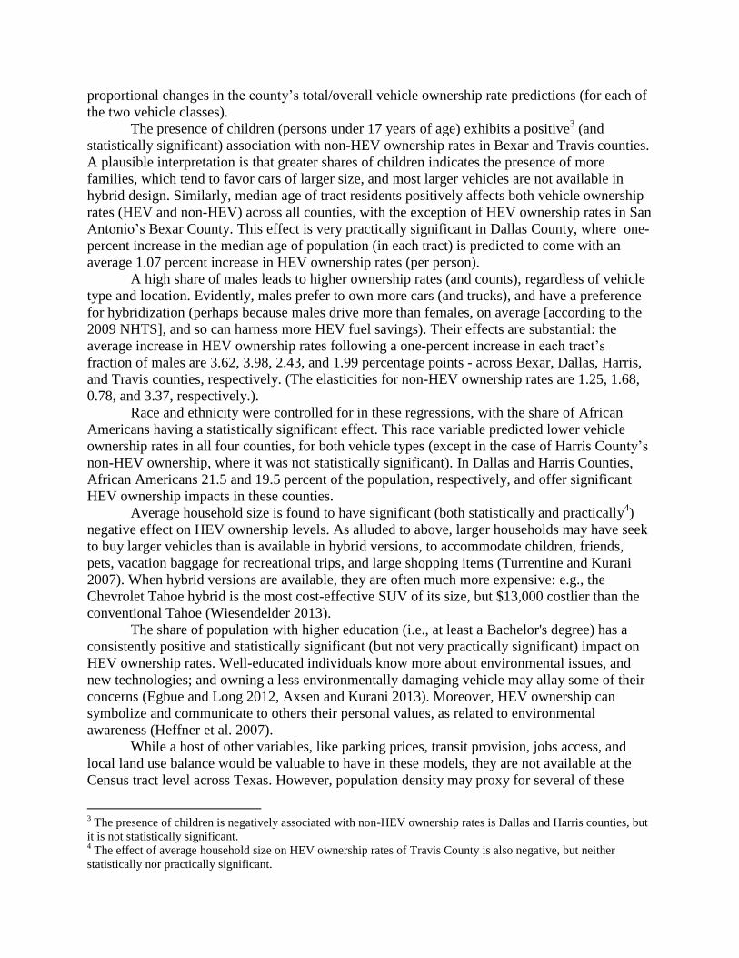
MODEL 2 RESULTS, FOR VEHICLE COUNTS BY FUEL ECONOMY CATEGORY

Table 3 shows Model 2’s parameter estimates. Since most HEVs fall into the third (“fuel

efficient”) vehicle category, some Model 2 coefficients are quite consistent with those estimated

for Model 1. The presence of children yields no significant effect on the adoption rates of fuel

efficient and inefficient vehicles, but has a positive and statistically significant effect on adoption

rates or counts of regular vehicles in two counties (for San Antonio and Austin locations). As in

Model 1, higher (median) ages (of tract residents) and shares of males have significantly positive

associations with all rates of vehicle ownership. Elasticity values of 1.10 to 2.17 (across the 4

counties) suggest that a higher share of males will have the greatest practical effect on the

purchase of fuel-efficient vehicles. A higher tract share of African Americans and higher

population density offer a negative association with vehicle ownership rates, regardless of fuel

efficiency level, presumably for the same reasons discussed above, in the context of Model 1

results. Population density remains rather a key here, with elasticity magnitudes ranging from

0.099 to 0.332 (for the categories of fuel-inefficient vehicles in Houston and regular vehicles in

Austin). Unlike many of the other covariates, density is a variable that almost has no bounds, and

can vary by orders of magnitude in U.S. data sets; thus, its cumulative effects on ownership,

vehicle choices, travel distances, and fuel use can be quite sizable.

Rising average household size is associated with lower ownership rates of fuel efficient

vehicles and higher fuel-inefficient vehicle adoption rates across all counties. As suggested

earlier, this may be attributed to larger households seeking more full-size vehicles (e.g., SUVs

and minivans), which typically have fuel economy ratings below 25 mi/gal (U.S. Department of

Energy 2014)8. As discussed earlier, for Model 1, higher education levels are positively

associated with higher ownership of fuel efficient vehicles and lower rates of fuel-inefficient

vehicles9.

The share of workers that commute by driving has positive and significant effects on all

three vehicle ownership rates in Bexar and Harris counties, as expected. (Dallas County has

negative coefficient estimates, but it is statistically and practically insignificant.) While average

household income is not a significant predictor, the share of high-income households has positive

(and significant except in Travis County) effects on ownership of more efficient vehicles in all

counties, with strongest responses for San Antonio’s and Dallas’ central counties (thanks to

elasticity estimates of 0.37 and 0.14, respectively). As noted earlier, this underscores the fact that

fuel-efficient vehicles tend to cost more than other vehicles and are more affordable for higher-

income households (Collins 2013, Prevedouros and Schofer 1992). Moreover, using the Travis

County model results, greater land use balance is associated with higher vehicle ownership rates

(in a statistically significant way), while greater employment density is correlated with lower

vehicle ownership rates (but this latter relationship is statistically significant only for rates of

fuel-efficient vehicles).

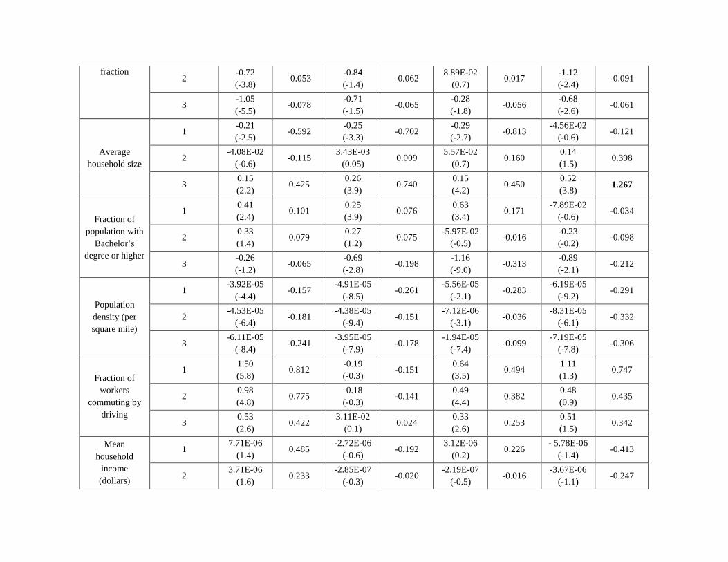
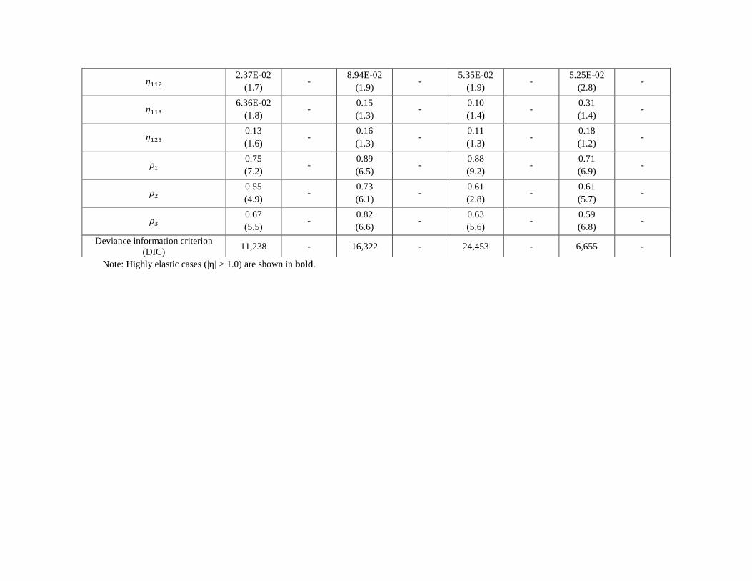
As before, spatial autocorrelation values (ρ’s) suggest that sizable spatial clustering

patterns exist in ownership rates, across all vehicle types (Keith 2012, Lane and Potter 2007).

Within the same census tract, correlation between fuel-efficient and regular-vehicle ownership

rates ( ) is not significant, but correlations between rates of fuel-efficient and inefficient

ownership ( ), and between rates of-fuel inefficient and regular vehicle ownership ( ) are

8 Austin’s Travis County yields the opposite sign on household size and education levels, but these estimates are not

significant (and may come from the presence of many college-age students in Travis County, who reside in Travis

County to attend U.T. Austin and other schools).

significant. Across census tracts, the spatially-lagged cross-correlations for all response pairs are

statistically insignificant and very low in magnitude, suggesting that levels of fuel efficient

vehicles in one census tract are not appreciably affected by adoption rates of other types of

vehicles in neighboring (first- and second-order contiguity) tracts.

TABLE 3. Model 2’s Parameter Estimates for Vehicle Ownership Counts at Different Fuel Economy Levels, using an MCAR

Specification

Variables Type

San Antonio (Bexar

County, n=361 tracts)

Dallas (Dallas County,

n=526 tracts)

Houston (Harris County,

n=780 tracts)

Austin (Travis County,

n=215 tracts)

Mean

(t-stat.) Elasticity

Mean

(t-stat.) Elasticity

Mean

(t-stat.) Elasticity

Mean

(t-stat.) Elasticity

Constant

Fuel Efficient

(1)

-3.82

(-5.7) -

-2.37

(-3.6) -

-2.84

(-5.3) -

-3.11

(-3.2) -

Regular

(2)

-2.41

(-4.5) -

-1.77

(-3.4) -

-2.08

(-6.3) -

-4.42

(-3.1) -

Fuel Inefficient

(3)

-4.60

(-8.6) -

-4.31

(-7.7) -

-4.24

(-11.4) -

-5.76

(-8.1) -

Fraction of

population 16

years old or

younger

1 2.46

(0.3) 0.593

1.20

(0.6) 0.287

0.52

(0.9) 0.126

0.29

(0.3) 0.062

2 1.72

(3.9) 0.415

-0.34

(-0.6) -0.0816

-0.77

(-0.4) -0.188

0.81

(2.1) 0.163

3 0.97

(0.6) 0.233

-2.64

(-0.9) -0.625

-0.79

(-0.9) -0.192

0.29

(0.4) 0.056

Median age of

population

(years)

1 -7.11E-03

(-0.3) -0.242

2.61E-03

(2.5) 0.088

1.11E-02

(2.7) 0.707

1.14E-02

(3.2) 0.678

2 6.98E-03

(1.6) 0.238

1.69E-02

(3.8) 0.574

1.26E-02

(4.4) 0.424

3.11E-02

(3.1) 0.715

3 1.79E-02

(4.1) 0.613

1.43E-02

(5.0) 0.425

1.69E-02

(5.3) 0.569

1.53E-02

(3.9) 0.502

Male fraction

1 2.24

(2.7) 1.101

3.78

(4.4) 1.893

2.62

(3.6) 1.551

3.11

(2.3) 2.178

2 1.56

(2.4) 0.872

2.56

(3.7) 1.085

1.51

(3.6) 0.858

3.67

(2.8) 1.871

3 2.07

(3.1) 0.821

2.60

(3.5) 0.933

2.44

(5.2) 0.852

6.31

(4.2) 1.562

African

American 1

-1.06

(-4.4) -0.098

-0.40

(-3.2) -0.086

-8.44E-02

(-4.9) -0.046

-1.62

(-3.3) -0.134

fraction 2

-0.72

(-3.8) -0.053

-0.84

(-1.4) -0.062

8.89E-02

(0.7) 0.017

-1.12

(-2.4) -0.091

3 -1.05

(-5.5) -0.078

-0.71

(-1.5) -0.065

-0.28

(-1.8) -0.056

-0.68

(-2.6) -0.061

Average

household size

1 -0.21

(-2.5) -0.592

-0.25

(-3.3) -0.702

-0.29

(-2.7) -0.813

-4.56E-02

(-0.6) -0.121

2 -4.08E-02

(-0.6) -0.115

3.43E-03

(0.05) 0.009

5.57E-02

(0.7) 0.160

0.14

(1.5) 0.398

3 0.15

(2.2) 0.425

0.26

(3.9) 0.740

0.15

(4.2) 0.450

0.52

(3.8) 1.267

Fraction of

population with

Bachelor’s

degree or higher

1 0.41

(2.4) 0.101

0.25

(3.9) 0.076

0.63

(3.4) 0.171

-7.89E-02

(-0.6) -0.034

2 0.33

(1.4) 0.079

0.27

(1.2) 0.075

-5.97E-02

(-0.5) -0.016

-0.23

(-0.2) -0.098

3 -0.26

(-1.2) -0.065

-0.69

(-2.8) -0.198

-1.16

(-9.0) -0.313

-0.89

(-2.1) -0.212

Population

density (per

square mile)

1 -3.92E-05

(-4.4) -0.157

-4.91E-05

(-8.5) -0.261

-5.56E-05

(-2.1) -0.283

-6.19E-05

(-9.2) -0.291

2 -4.53E-05

(-6.4) -0.181

-4.38E-05

(-9.4) -0.151

-7.12E-06

(-3.1) -0.036

-8.31E-05

(-6.1) -0.332

3 -6.11E-05

(-8.4) -0.241

-3.95E-05

(-7.9) -0.178

-1.94E-05

(-7.4) -0.099

-7.19E-05

(-7.8) -0.306

Fraction of

workers

commuting by

driving

1 1.50

(5.8) 0.812

-0.19

(-0.3) -0.151

0.64

(3.5) 0.494

1.11

(1.3) 0.747

2 0.98

(4.8) 0.775

-0.18

(-0.3) -0.141

0.49

(4.4) 0.382

0.48

(0.9) 0.435

3 0.53

(2.6) 0.422

3.11E-02

(0.1) 0.024

0.33

(2.6) 0.253

0.51

(1.5) 0.342

Mean

household

income

(dollars)

1 7.71E-06

(1.4) 0.485

-2.72E-06

(-0.6) -0.192

3.12E-06

(0.2) 0.226

- 5.78E-06

(-1.4) -0.413

2 3.71E-06

(1.6) 0.233

-2.85E-07

(-0.3) -0.020

-2.19E-07

(-0.5) -0.016

-3.67E-06

(-1.1) -0.247

3 3.09E-06

(2.2) 0.194

-4.03E-06

(-0.4) -0.284

-3.37E-06

(-0.3) -0.245

-1.98E-06

(-1.3) -0.156

Fraction of

households with

income over

$100,000

1 2.22

(4.9) 0.370

0.74

(2.9) 0.142

0.25

(4.7) 0.053

3.13E-02

(0.8) 0.008

2 -1.21

(-3.4) -0.202

-0.72

(-2.3) -0.137

2.19E-02

(0.2) 0.004

-8.12E-02

(-0.1) -0.023

3 -0.82

(-2.3) -0.137

-0.71

(-2.1) -0.126

-1.43E-02

(-0.08) -0.003

-0.91

(-1.5) -0.167

Fraction of

families below

poverty level

1 -0.54

(-2.1) -0.078

-0.84

(-3.2) -0.129

-0.81

(-4.4) -0.123

-0.33

(-0.4) -0.042

2 -0.44

(-3.1) -0.064

3.81E-02

(0.2) 0.006

-0.30

(-2.6) -0.046

-0.25

(-2.9) -0.034

3 -0.10

(-0.5) -0.015

0.91

(4.1) 0.139

-0.10

(-0.8) -0.016

0.16

(0.2) 0.025

Land use

balance

1 - - - - - - 0.21

(2.1) 0.322

2 - - - - - - 0.11

(2.9) 0.412

3 - - - - - - 0.34

(1.9) 0.335

Employment

density

1 - - - - - - -3.32E-04

(-2.1) -0.112

2 - - - - - - -8.27E-05

(-0.9) -0.063

3 - - - - - - -6.11E-05

(-0.3) -0.045

0.32

(1.4) -

0.39

(1.4) -

0.36

(1.3) -

0.45

(1.6) -

0.40

(2.0) -

0.49

(4.1) -

0.52

(3.9) -

0.56

(4.1) -

0.59

(2.9) -

0.58

(5.0) -

0.67

(3.6) -

0.61

(3.6) -

Note: Highly elastic cases (|| > 1.0) are shown in bold.

2.37E-02

(1.7) -

8.94E-02

(1.9) -

5.35E-02

(1.9) -

5.25E-02

(2.8) -

6.36E-02

(1.8) -

0.15

(1.3) -

0.10

(1.4) -

0.31

(1.4) -

0.13

(1.6) -

0.16

(1.3) -

0.11

(1.3) -

0.18

(1.2) -

0.75

(7.2) -

0.89

(6.5) -

0.88

(9.2) -

0.71

(6.9) -

0.55

(4.9) -

0.73

(6.1) -

0.61

(2.8) -

0.61

(5.7) -

0.67

(5.5) -

0.82

(6.6) -

0.63

(5.6) -

0.59

(6.8) -

Deviance information criterion

(DIC) 11,238 - 16,322 - 24,453 - 6,655 -

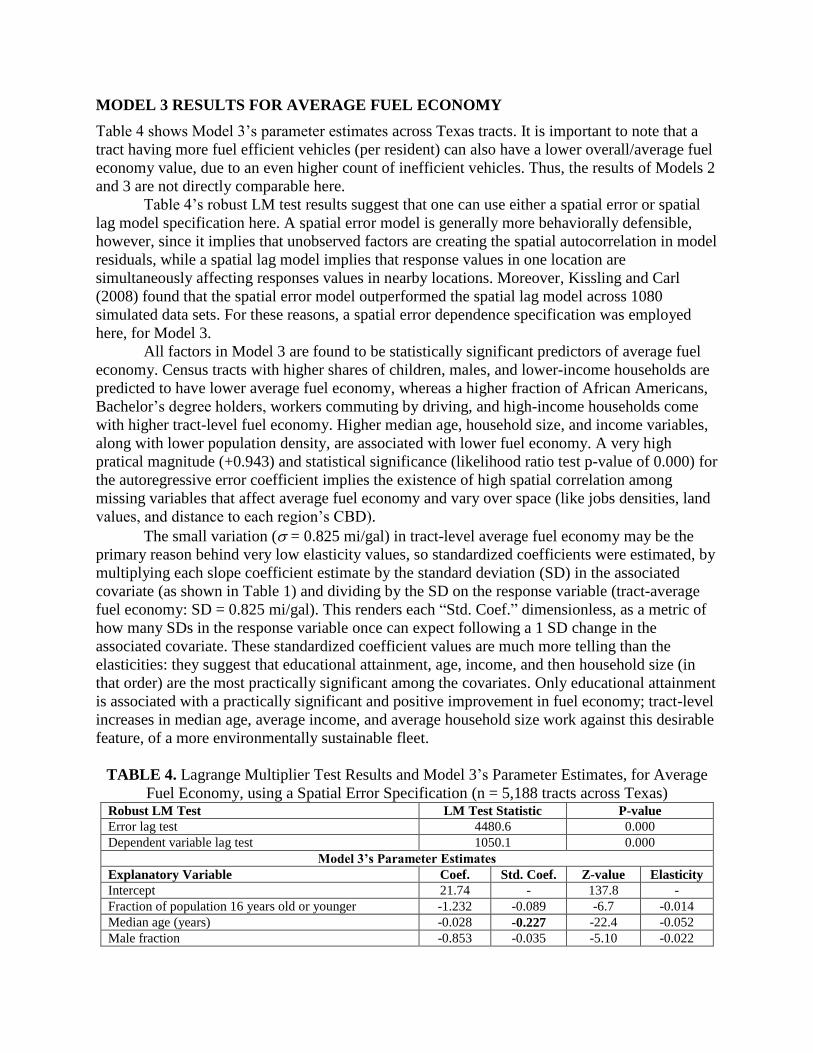
MODEL 3 RESULTS FOR AVERAGE FUEL ECONOMY

Table 4 shows Model 3’s parameter estimates across Texas tracts. It is important to note that a

tract having more fuel efficient vehicles (per resident) can also have a lower overall/average fuel

economy value, due to an even higher count of inefficient vehicles. Thus, the results of Models 2

and 3 are not directly comparable here.

Table 4’s robust LM test results suggest that one can use either a spatial error or spatial

lag model specification here. A spatial error model is generally more behaviorally defensible,

however, since it implies that unobserved factors are creating the spatial autocorrelation in model

residuals, while a spatial lag model implies that response values in one location are

simultaneously affecting responses values in nearby locations. Moreover, Kissling and Carl

(2008) found that the spatial error model outperformed the spatial lag model across 1080

simulated data sets. For these reasons, a spatial error dependence specification was employed

here, for Model 3.

All factors in Model 3 are found to be statistically significant predictors of average fuel

economy. Census tracts with higher shares of children, males, and lower-income households are

predicted to have lower average fuel economy, whereas a higher fraction of African Americans,

Bachelor’s degree holders, workers commuting by driving, and high-income households come

with higher tract-level fuel economy. Higher median age, household size, and income variables,

along with lower population density, are associated with lower fuel economy. A very high

pratical magnitude (+0.943) and statistical significance (likelihood ratio test p-value of 0.000) for

the autoregressive error coefficient implies the existence of high spatial correlation among

missing variables that affect average fuel economy and vary over space (like jobs densities, land

values, and distance to each region’s CBD).

The small variation ( = 0.825 mi/gal) in tract-level average fuel economy may be the

primary reason behind very low elasticity values, so standardized coefficients were estimated, by

multiplying each slope coefficient estimate by the standard deviation (SD) in the associated

covariate (as shown in Table 1) and dividing by the SD on the response variable (tract-average

fuel economy: SD = 0.825 mi/gal). This renders each “Std. Coef.” dimensionless, as a metric of

how many SDs in the response variable once can expect following a 1 SD change in the

associated covariate. These standardized coefficient values are much more telling than the

elasticities: they suggest that educational attainment, age, income, and then household size (in

that order) are the most practically significant among the covariates. Only educational attainment

is associated with a practically significant and positive improvement in fuel economy; tract-level

increases in median age, average income, and average household size work against this desirable

feature, of a more environmentally sustainable fleet.

TABLE 4. Lagrange Multiplier Test Results and Model 3’s Parameter Estimates, for Average

Fuel Economy, using a Spatial Error Specification (n = 5,188 tracts across Texas) Robust LM Test LM Test Statistic P-value

Error lag test 4480.6 0.000

Dependent variable lag test 1050.1 0.000

Model 3’s Parameter Estimates

Explanatory Variable Coef. Std. Coef. Z-value Elasticity

Intercept 21.74 - 137.8 -

Fraction of population 16 years old or younger -1.232 -0.089 -6.7 -0.014

Median age (years) -0.028 -0.227 -22.4 -0.052

Male fraction -0.853 -0.035 -5.10 -0.022

African American fraction 0.681 0.136 14.0 0.004

Average household size (# persons) -0.298 -0.180 -12.6 -0.042

Fraction of population with Bachelor's degree or higher 1.120 0.259 16.1 0.014

Population density (per square mile) 2.55E-05 0.102 12.6 0.004

Fraction of workers commuting by driving 0.199 0.022 3.2 0.008

Mean household income (dollars per year, in 2010) -5.1E-06 -0.225 -13.8 -0.018

Fraction of households with income over $100,000 0.327 0.065 3.5 0.003

Fraction of families below poverty level -0.443 -0.066 -7.3 -0.003

Simultaneous autoregressive error coefficient (λ) 0.943 - 140.2 -

Likelihood ratio test on λ 4673.2 (p-value = 0.000)

Akaike information criterion (AIC) 3368.5 (vs. 8037.9 for OLS model)

Note: Practically significant covariates have their standardized coefficients shown in bold.

CONCLUSIONS

This study employed a Poisson-lognormal CAR model to anticipate tract-level counts of HEVs

and non-HEVs, fuel efficient and inefficient vehicles across Texas’ most populous cities, along

with a spatial error model for average fuel economy across all Texas tracts. Model results

identify demographic (including population density) factors that most affect HEV ownership

rates, vehicle ownership by fuel economy categories, and the average fuel economy of registered

LDVs in each tract.

Results of the count models suggest that household size, resident gender, household

income, jobs density, and education levels are key predictors for HEV adoption rates and fuel

economy choices, though average fuel economy does not vary much across tracts (with = 19.2,

and = 0.82 mi/gal). It appears that larger households tend to not purchase HEVs or other fuel

efficient vehicles, presumably due to a preference for larger vehicles (e.g., SUVs and minivans

[Kockelman and Zhao 2000]), and possibly due to higher up-front pricing of fuel-saving

technologies. Higher population densities are associated with statistically significantly lower

vehicle ownership rates (regardless of vehicle type), presumably due to better access options to

destinations without a private vehicle and due to more parking challenges or costs. All three

model specifications exhibit high (and statistically significant) spatial autocorrelations and local

(within a tract) cross-response correlations in unobserved attributes (like concern for the

environment, parking challenges, manufacturers’ marketing campaigns, locations of vehicle

dealerships, and access to neighbors and friends who already own HEVs and/or vehicles that

enjoy higher fuel economy). While the Bayesian sampling methods and the MCAR model

specification are not familiar techniques for many data analysts, neglect of such correlations can

result in biased parameter estimates. The spatial error model is more accessible to a variety of

potential users (and exists in various software programs); it also can handle much larger data sets

(though it effectively requires a continuous response variable).

Although modeling vehicle-choice behavior at the level of individuals or households,

with disaggregate data, can also prove quite informative for understanding HEV ownership, such

data are obtained for small samples of the population, and only sporadically. (For example,

typically 1 percent or fewer households in a region provide data for a regional household travel

survey, which is undertaken every 5 to 10 years. In contrast, DMV records contain all registered

vehicles, continuously in time.) This study demonstrates how one can use rigorous spatial

modeling methods at the census tract or other levels to understand vehicle ownership choices and

fuel economy relationships across counties and a large state.

Opportunities for future research in this area are many. For example, while it is often

challenging to obtain tract level data of various land use, transit provision, and other relevant

variables across a state like Texas, inclusion of such covariates will provide even more insight

for planners, policy-makers, automobile manufacturers, and other interested readers. Access to

count data on PEVs (as these become non-negligible), average vehicle age information, and

other features of DMV databases will also inform these analyses, while helping chart a course for

charging infrastructure investments and other decisions. Vehicle age is relevant, for example,

because lower-income households are less likely to buy new vehicles, and so may be holding less

fuel efficient vehicles as rising Corporate Average Fuel Economy standards ensure the nation’s

new-sales fleet becomes more efficient. This study also was able to estimate rather complex

MCAR count models for only subsets of Texas tracts, due to computing limitations; advances in

Bayesian estimation and software programming may eventually permit estimation of such

models for much larger data sets.

While ownership of an HEV does not require special charging stations, larger power

transformers, or very large batteries on board, their rising presence does affect future sales, of

vehicles and gasoline, as well as state and federal gas tax receipts, air quality, and energy

security. Since early adopters of HEVs are likely to be more sustainability-minded and

technology savvy than others, on average; so their heavy presence in various neighborhoods may

well be a strong signal for the early adoption and longer-term registration numbers of plug-in

EVs in those same locations. Greater understanding of the factors causing spatial clustering in all

EVs’ adoption rates can help shape environmental policy, infrastructure planning, and vehicle

marketing.

ACKNOWLEDGEMENTS

The authors are thankful to the NSF Industry-University Research Center titled “Efficient

Vehicles and Sustainable Transportation Systems” for financially supporting this research, and to

several anonymous reviewers for their suggestions. They are also obliged to Texas A&M

University’s Prof. Steve Puller for providing access to the coded and aggregate vehicle

registration data, and to the Texas Department of Motor Vehicles for permitting this access.

REFERENCES

Anselin, L. (1988) Spatial Econometrics: Methods and Models. Dordrecht: Kluwer Academic

Publishers.

Anselin, L. (2003) An introduction to spatial regression analysis in R. University of Illinois,

Urbana-Champaign. Retrieved from: https://geodacenter.asu.edu/drupal_files/spdepintro.pdf

(October 26, 2014).

Anselin, L., Bera, A. K., Florax, R., and Yoon, M. J. (1996) Simple diagnostic tests for spatial

dependence. Regional Science and Urban Economics, 26(1):77-104.

Axsen, J., and Kurani, K. S. (2013) Hybrid, Plug-in Hybrid, or Electric-What do Car Buyers

Want? Energy Policy 61: 532-543.

Axsen, J., and Kurani, K. S. (2011) Interpersonal influence in the early Plug-in Hybrid Market:

Observing Social Interactions with an Exploratory Multi-Method Approach. Transportation

Research Part D: Transport and Environment 16(2): 150-159.

Caulfield, B., Farrell, S., and McMahon, B. (2010) Examining Individuals Preferences for

Hybrid Electric and Alternatively Fuelled Vehicles. Transport Policy 17(6): 381-387.

Cervero, R., and Kockelman, K. (1997) Travel demand and the 3Ds: density, diversity, and

design. Transportation Research Part D 2(3): 199-219.

Chen, T. D., Wang, Y., and Kockelman, K. M. (2014) Where are the Electric Vehicles? A

Spatial Model for Vehicle-Choice Count Data. Forthcoming in Journal of Transport Geography.

Chu, Y. L. (2002) Automobile Ownership Analysis using Ordered Probit Models.

Transportation Research Record: Journal of the Transportation Research Board 1805(1): 60-67.

Collins A.P. (2013) New Fuel Standards: Costlier Cars, but Less Expensive to Run. Retrieved

from: http://www.csmonitor.com/Business/In-Gear/2013/1005/New-fuel-standards-Costlier-cars-

but-less-expensive-to-run (July 4, 2014)

Cressie, N.A.C. (1993) Statistics for Spatial Data. Wiley Series in Probability and Mathematical

Statistics. Wiley, New York.

Dijk, M., Orsato, R. J., and Kemp, R. (2013) The Emergence of an Electric Mobility

Trajectory. Energy Policy 52: 135-145.

Egbue, O., and Long, S (2012) Barriers to Widespread Adoption of Electric Vehicles: An

Analysis of Consumer Attitudes and Perceptions. Energy Policy 48: 717-729.

EVs Roll (2014) Hybrid Car Statistics. Retrieved from:

http://www.evsroll.com/Hybrid_Car_Statistics.html# (June 12, 2014)

Gallagher, K. S., and Muehlegger, E. (2011) Giving Green to Get Green? Incentives and

Consumer Adoption of Hybrid Vehicle Technology. Journal of Environmental Economics and

Management 61(1): 1-15

Greene, D. L., Evans, D. H., and Hiestand, J. (2013) Survey Evidence on the Willingness of US

Consumers to Pay for Automotive Fuel Economy. Energy Policy 61: 1539-1550.

He, L., Chen, W., and Conzelmann, G. (2012) Impact of Vehicle Usage on Consumer Choice of

Hybrid Electric Vehicles. Transportation Research Part D: Transport and Environment 17(3):

208-214.

Heffner, R. R., Kurani, K. S., and Turrentine, T. S. (2007) Symbolism in California’s Early

Market for Hybrid Electric Vehicles. Transportation Research Part D: Transport and

Environment 12(6): 396-413.

Jenn, A., Azevedo, I. L., and Ferreira, P. (2013) The Impact of Federal Incentives on the

Adoption of Hybrid Electric Vehicles in the United States. Energy Economics 40: 936-942.

Keith, D. R. (2012) Essays on the Dynamics of Alternative Fuel Vehicle Adoption: Insights from

the Market for Hybrid-electric Vehicles in the United States. Doctoral dissertation in

Engineering Systems Division. Massachusetts Institute of Technology.

Keith, D., Sterman, J., and Struben, J. (2012) Understanding Spatiotemporal Patterns of Hybrid-

Electric Vehicle Adoption in the United States. In Transportation Research Board 91st Annual

Meeting (No. 12-4164).

Kissling, W. D., and Carl, G. (2008) Spatial Autocorrelation and the Selection of Simultaneous

Autoregressive Models. Global Ecology and Biogeography 17(1): 59-71.

Kodjak, D. (2012) Consumer Acceptance of Electric Vehicles in the United States. Retrieved

from: http://www.epa.gov/oar/caaac/mstrs/dec2012/kodjak.pdf (June 16, 2014)

Koo, Y., Kim, C. S., Hong, J., Choi, I. J., and Lee, J. (2012) Consumer Preferences for

Automobile Energy-Efficiency Grades. Energy Economics 34(2): 446-451.

Lane, B., and Potter, S. (2007) The Adoption of Cleaner Vehicles in the UK: Exploring the

Consumer Attitude–action Gap. Journal of Cleaner Production 15(11): 1085–1092.

Li, X., Clark, C. D., Jensen, K. L., Yen, S. T., and English, B. C. (2013) Consumer Purchase

Intentions for Flexible-Fuel and Hybrid-Electric Vehicles. Transportation Research Part D:

Transport and Environment 18: 9-15.

Liu, Y. (2014), Household Demand and Willingness to Pay for Hybrid Vehicles. Energy

Economics 44: 191-197.

Murakami, E., and Young, J. (1997) Daily Travel by Persons with Low Income, US Federal

Highway Administration.

Musti, S., and Kockelman, K. (2011) Evolution of the Household Vehicle Fleet: Anticipating

Fleet Composition and PHEV Adoption in Austin, Texas. Transportation Research Part A 45

(8): 707-720.

Paul, B., Kockelman, K., Musti, S. (2011) Evolution of the Light-Duty-Vehicle Fleet:

Anticipating Adoption of Plug-In Hybrid Electric Vehicles and Greenhouse Gas Emissions

Across the U.S. Fleet. Transportation Research Record No. 2252: 107-117.

Potoglou, D., and Kanaroglou, P. S. (2008) Modeling Car Ownership in Urban Areas: A Case

Study of Hamilton, Canada. Journal of Transport Geography 16(1): 42-54.

Prevedouros, P.D., and Schofer, J.L. (1992) Factors Affecting Automobile Ownership and Use.

Transportation Research Record 1364:152–16.

Tuttle, D., and Kockelman, K. (2012) Electrified Vehicle Technology Trends, Infrastructure

Implications, and Cost Comparisons. J of the Transportation Research Forum 51 (1): 35-51.

Turrentine, T. S., and Kurani, K. S. (2007) Car Buyers and Fuel Economy? Energy Policy 35(2):

1213-1223.

United States Census Bureau (2010) Census Tract Relationship File. Retrieved from:

https://www.census.gov/geo/maps-data/data/relationship.html (June 16, 2014)

U.S. Department of Energy (2014) Best and Worst MI/GAL Trucks, Vans and SUVs.

Wall, M. M. (2004) A Close Look at the Spatial Structure Implied by the CAR and SAR Models.

Journal of Statistical Planning and Inference 121(2): 311-324.

Wang, Y., and Kockelman, K. M. (2013) A Poisson-lognormal Conditional-Autoregressive

Model for Multivariate Spatial Analysis of Pedestrian Crash Counts across Neighborhoods.

Accident Analysis & Prevention 60: 71-84.

Wiesendelder J. (2013) Best Hybrids for the Money 2013.Retrieved from:

http://blogs.cars.com/kickingtires/2013/04/best-hybrids-for-the-money-2013.html (June 2, 2014).

Zhao, Y., and Kockelman, K. (2000) Behavioral Distinctions: The Use of Light-Duty Trucks and

Passenger Cars. Journal of Transportation and Statistics 3 (3): 47-60.