Huygens - Experimental Oncology Graduate Study

Scientific Volume Imaging B.V.

Huygens Essential

User Guide for version 3.5

Huygens Essential

User Guide for version 3.5

Scientific Volume Imaging B.V.

Copyright © 1995-2009 by Scientific Volume Imaging B.V.All rights reserved

Cover illustration: Macrophage recorded by Dr. James Evans (White-head Institute, MIT, Boston MA, USA) using widefield microscopy, as deconvolved with Huygens®. Stained for tubulin (yellow/green), actin (red) and the nucleus (DAPI, blue).

Mailing Address Scientific Volume Imaging B.V.Laapersveld 631213 VB HilversumThe Netherlands

Phone +31 35 6421626Fax +31 35 6837971E-mail [email protected]

URL http://www.svi.nl/

Contents

CHAPTER 1 Introduction. . . . . . . . . . . . . . . . . . . . . . . . . . . . . . . . . . . . . . 1

CHAPTER 2 Installation . . . . . . . . . . . . . . . . . . . . . . . . . . . . . . . . . . . . . . 3Microsoft Windows . . . . . . . . . . . . . . . . . . . . . . . . . . . . . . . . . . . . . . . . . . . . . . . . . . . . .3Microsoft Windows 64 bit Edition . . . . . . . . . . . . . . . . . . . . . . . . . . . . . . . . . . . . . . . . .3Mac OS X . . . . . . . . . . . . . . . . . . . . . . . . . . . . . . . . . . . . . . . . . . . . . . . . . . . . . . . . . . . . .3Linux (Debian) . . . . . . . . . . . . . . . . . . . . . . . . . . . . . . . . . . . . . . . . . . . . . . . . . . . . . . . .3Linux (RPM) . . . . . . . . . . . . . . . . . . . . . . . . . . . . . . . . . . . . . . . . . . . . . . . . . . . . . . . . . .4After the Installation . . . . . . . . . . . . . . . . . . . . . . . . . . . . . . . . . . . . . . . . . . . . . . . . . . . .4The License String . . . . . . . . . . . . . . . . . . . . . . . . . . . . . . . . . . . . . . . . . . . . . . . . . . . . . .4Updating the Software. . . . . . . . . . . . . . . . . . . . . . . . . . . . . . . . . . . . . . . . . . . . . . . . . . .6Removing the Software . . . . . . . . . . . . . . . . . . . . . . . . . . . . . . . . . . . . . . . . . . . . . . . . . .7System Requirements for Huygens Essential . . . . . . . . . . . . . . . . . . . . . . . . . . . . . . . .7Support on Installation . . . . . . . . . . . . . . . . . . . . . . . . . . . . . . . . . . . . . . . . . . . . . . . . . .8

CHAPTER 3 The Image Restoration Process . . . . . . . . . . . . . . . . . . . . . . . 9The Processing Stages in the Wizard . . . . . . . . . . . . . . . . . . . . . . . . . . . . . . . . . . . . . . .9Loading an Image . . . . . . . . . . . . . . . . . . . . . . . . . . . . . . . . . . . . . . . . . . . . . . . . . . . . . .9Verifying Microscopic Parameters . . . . . . . . . . . . . . . . . . . . . . . . . . . . . . . . . . . . . . . 10The Intelligent Cropper. . . . . . . . . . . . . . . . . . . . . . . . . . . . . . . . . . . . . . . . . . . . . . . . 12The Image Histogram . . . . . . . . . . . . . . . . . . . . . . . . . . . . . . . . . . . . . . . . . . . . . . . . . 13Estimating the Average Background . . . . . . . . . . . . . . . . . . . . . . . . . . . . . . . . . . . . . 14The Deconvolution Stage . . . . . . . . . . . . . . . . . . . . . . . . . . . . . . . . . . . . . . . . . . . . . . 15Finishing or Restarting a Deconvolution Run . . . . . . . . . . . . . . . . . . . . . . . . . . . . . 16Multi-channel Images . . . . . . . . . . . . . . . . . . . . . . . . . . . . . . . . . . . . . . . . . . . . . . . . . 16Z-drift Correcting for Time Series . . . . . . . . . . . . . . . . . . . . . . . . . . . . . . . . . . . . . . . 17Saving the Result . . . . . . . . . . . . . . . . . . . . . . . . . . . . . . . . . . . . . . . . . . . . . . . . . . . . . 17Using a Measured PSF. . . . . . . . . . . . . . . . . . . . . . . . . . . . . . . . . . . . . . . . . . . . . . . . . 17

Huygens Essential User Guide for version 3.5 i

CHAPTER 4 The Batch Processor. . . . . . . . . . . . . . . . . . . . . . . . . . . . . . . 19The Batch Processor Window. . . . . . . . . . . . . . . . . . . . . . . . . . . . . . . . . . . . . . . . . . . 19Usage. . . . . . . . . . . . . . . . . . . . . . . . . . . . . . . . . . . . . . . . . . . . . . . . . . . . . . . . . . . . . . . 20Menus . . . . . . . . . . . . . . . . . . . . . . . . . . . . . . . . . . . . . . . . . . . . . . . . . . . . . . . . . . . . . . 23

CHAPTER 5 The Twin Slicer . . . . . . . . . . . . . . . . . . . . . . . . . . . . . . . . . . 25Using the Slicer in Basic Mode . . . . . . . . . . . . . . . . . . . . . . . . . . . . . . . . . . . . . . . . . . 26Using the Slicer in Advanced Mode . . . . . . . . . . . . . . . . . . . . . . . . . . . . . . . . . . . . . . 28Measurement . . . . . . . . . . . . . . . . . . . . . . . . . . . . . . . . . . . . . . . . . . . . . . . . . . . . . . . . 30

CHAPTER 6 The MIP Renderer . . . . . . . . . . . . . . . . . . . . . . . . . . . . . . . . 33Basic Usage. . . . . . . . . . . . . . . . . . . . . . . . . . . . . . . . . . . . . . . . . . . . . . . . . . . . . . . . . . 33Advanced Usage. . . . . . . . . . . . . . . . . . . . . . . . . . . . . . . . . . . . . . . . . . . . . . . . . . . . . . 35Simple Animations . . . . . . . . . . . . . . . . . . . . . . . . . . . . . . . . . . . . . . . . . . . . . . . . . . . 35

CHAPTER 7 The SFP Renderer . . . . . . . . . . . . . . . . . . . . . . . . . . . . . . . . 37Basic Usage. . . . . . . . . . . . . . . . . . . . . . . . . . . . . . . . . . . . . . . . . . . . . . . . . . . . . . . . . . 37Advanced Usage. . . . . . . . . . . . . . . . . . . . . . . . . . . . . . . . . . . . . . . . . . . . . . . . . . . . . . 39Simple Animations . . . . . . . . . . . . . . . . . . . . . . . . . . . . . . . . . . . . . . . . . . . . . . . . . . . 40

CHAPTER 8 The Surface Renderer . . . . . . . . . . . . . . . . . . . . . . . . . . . . . 41Basic Usage. . . . . . . . . . . . . . . . . . . . . . . . . . . . . . . . . . . . . . . . . . . . . . . . . . . . . . . . . . 42Advanced Usage. . . . . . . . . . . . . . . . . . . . . . . . . . . . . . . . . . . . . . . . . . . . . . . . . . . . . . 43Simple Animations . . . . . . . . . . . . . . . . . . . . . . . . . . . . . . . . . . . . . . . . . . . . . . . . . . . 44

CHAPTER 9 The Movie Maker . . . . . . . . . . . . . . . . . . . . . . . . . . . . . . . . 47An Overview . . . . . . . . . . . . . . . . . . . . . . . . . . . . . . . . . . . . . . . . . . . . . . . . . . . . . . . . 47Creating and Adjusting Keyframes . . . . . . . . . . . . . . . . . . . . . . . . . . . . . . . . . . . . . . 48Using the Storyboard. . . . . . . . . . . . . . . . . . . . . . . . . . . . . . . . . . . . . . . . . . . . . . . . . . 49Working with Movie Projects . . . . . . . . . . . . . . . . . . . . . . . . . . . . . . . . . . . . . . . . . . . 50Using the Timeline. . . . . . . . . . . . . . . . . . . . . . . . . . . . . . . . . . . . . . . . . . . . . . . . . . . . 50Advanced Topics . . . . . . . . . . . . . . . . . . . . . . . . . . . . . . . . . . . . . . . . . . . . . . . . . . . . . 51

CHAPTER 10 Introducion to the Object Analyzer . . . . . . . . . . . . . . . . . . . 53Starting the Object Analyzer . . . . . . . . . . . . . . . . . . . . . . . . . . . . . . . . . . . . . . . . . . . 53Segmenting the Objects: Setting the Threshold . . . . . . . . . . . . . . . . . . . . . . . . . . . . 55Interaction with the Objects . . . . . . . . . . . . . . . . . . . . . . . . . . . . . . . . . . . . . . . . . . . . 57Render Pipes . . . . . . . . . . . . . . . . . . . . . . . . . . . . . . . . . . . . . . . . . . . . . . . . . . . . . . . . 58Object Statistics . . . . . . . . . . . . . . . . . . . . . . . . . . . . . . . . . . . . . . . . . . . . . . . . . . . . . . 59

ii Huygens Essential User Guide for version 3.5

Storing your Results . . . . . . . . . . . . . . . . . . . . . . . . . . . . . . . . . . . . . . . . . . . . . . . . . . 63Further Reading. . . . . . . . . . . . . . . . . . . . . . . . . . . . . . . . . . . . . . . . . . . . . . . . . . . . . . 63

CHAPTER 11 Object Analyzer Geometry Measurements . . . . . . . . . . . . . 65Iso-surface . . . . . . . . . . . . . . . . . . . . . . . . . . . . . . . . . . . . . . . . . . . . . . . . . . . . . . . . . . 65Principal Axis. . . . . . . . . . . . . . . . . . . . . . . . . . . . . . . . . . . . . . . . . . . . . . . . . . . . . . . . 65Length and width. . . . . . . . . . . . . . . . . . . . . . . . . . . . . . . . . . . . . . . . . . . . . . . . . . . . . 65Sphericity . . . . . . . . . . . . . . . . . . . . . . . . . . . . . . . . . . . . . . . . . . . . . . . . . . . . . . . . . . . 66Aspect Ratio . . . . . . . . . . . . . . . . . . . . . . . . . . . . . . . . . . . . . . . . . . . . . . . . . . . . . . . . . 67More Parameters and Filtering . . . . . . . . . . . . . . . . . . . . . . . . . . . . . . . . . . . . . . . . . . 67

CHAPTER 12 Object Analyzer Component Reference. . . . . . . . . . . . . . . . 69Main window components . . . . . . . . . . . . . . . . . . . . . . . . . . . . . . . . . . . . . . . . . . . . . 70

CHAPTER 13 The Colocalization Analyzer. . . . . . . . . . . . . . . . . . . . . . . . 85Iso-colocalization object analysis . . . . . . . . . . . . . . . . . . . . . . . . . . . . . . . . . . . . . . . . 85How to use the Colocalization Analyzer . . . . . . . . . . . . . . . . . . . . . . . . . . . . . . . . . . 86Backgrounds vs. thresholds in colocalization . . . . . . . . . . . . . . . . . . . . . . . . . . . . . . 88

CHAPTER 14 The PSF Distiller . . . . . . . . . . . . . . . . . . . . . . . . . . . . . . . . . 89The Processing Stages in the Wizard . . . . . . . . . . . . . . . . . . . . . . . . . . . . . . . . . . . . . 89Averaging Stage . . . . . . . . . . . . . . . . . . . . . . . . . . . . . . . . . . . . . . . . . . . . . . . . . . . . . . 90Distillation Stage . . . . . . . . . . . . . . . . . . . . . . . . . . . . . . . . . . . . . . . . . . . . . . . . . . . . . 91Assembly Stage . . . . . . . . . . . . . . . . . . . . . . . . . . . . . . . . . . . . . . . . . . . . . . . . . . . . . . 91Beads Suited for PSF Distillation . . . . . . . . . . . . . . . . . . . . . . . . . . . . . . . . . . . . . . . . 92

CHAPTER 15 Establishing Image Parameters . . . . . . . . . . . . . . . . . . . . . . 93Image Size. . . . . . . . . . . . . . . . . . . . . . . . . . . . . . . . . . . . . . . . . . . . . . . . . . . . . . . . . . . 93Signal to Noise Ratio . . . . . . . . . . . . . . . . . . . . . . . . . . . . . . . . . . . . . . . . . . . . . . . . . . 93Black Level . . . . . . . . . . . . . . . . . . . . . . . . . . . . . . . . . . . . . . . . . . . . . . . . . . . . . . . . . . 95Sampling Density. . . . . . . . . . . . . . . . . . . . . . . . . . . . . . . . . . . . . . . . . . . . . . . . . . . . . 95Computing the Backprojected Pinhole Radius and Distance . . . . . . . . . . . . . . . . . 96

CHAPTER 16 Improving Image Quality . . . . . . . . . . . . . . . . . . . . . . . . . 101Data Acquisition Pitfalls . . . . . . . . . . . . . . . . . . . . . . . . . . . . . . . . . . . . . . . . . . . . . . 101Deconvolution Improvements . . . . . . . . . . . . . . . . . . . . . . . . . . . . . . . . . . . . . . . . . 104

CHAPTER 17 Appendix . . . . . . . . . . . . . . . . . . . . . . . . . . . . . . . . . . . . . . 105License String Details . . . . . . . . . . . . . . . . . . . . . . . . . . . . . . . . . . . . . . . . . . . . . . . . 105

Huygens Essential User Guide for version 3.5 iii

The Point Spread Function . . . . . . . . . . . . . . . . . . . . . . . . . . . . . . . . . . . . . . . . . . . . 106Quality Factor . . . . . . . . . . . . . . . . . . . . . . . . . . . . . . . . . . . . . . . . . . . . . . . . . . . . . . 107File Series . . . . . . . . . . . . . . . . . . . . . . . . . . . . . . . . . . . . . . . . . . . . . . . . . . . . . . . . . . 107Adjusting the Global Color Scheme. . . . . . . . . . . . . . . . . . . . . . . . . . . . . . . . . . . . . 108Hue Selector . . . . . . . . . . . . . . . . . . . . . . . . . . . . . . . . . . . . . . . . . . . . . . . . . . . . . . . . 109Image Statistics . . . . . . . . . . . . . . . . . . . . . . . . . . . . . . . . . . . . . . . . . . . . . . . . . . . . . 109Setting the Coverslip Position . . . . . . . . . . . . . . . . . . . . . . . . . . . . . . . . . . . . . . . . . 110Excitation Beam Overfill Factor. . . . . . . . . . . . . . . . . . . . . . . . . . . . . . . . . . . . . . . . 111Brightfield Images . . . . . . . . . . . . . . . . . . . . . . . . . . . . . . . . . . . . . . . . . . . . . . . . . . . 112Support and Contact Information . . . . . . . . . . . . . . . . . . . . . . . . . . . . . . . . . . . . . . 112

iv Huygens Essential User Guide for version 3.5

CHAPTER 1 Introduction

Huygens Essential is an image processing software package tailored for restoration, visu-alization and analysis of microscopic images. Its wizard driven user interface guides through the process of deconvolving images from light microscopes. Huygens Essential is able to deconvolve a wide variety of images ranging from 2D widefield images to 4D multi-channel multi-photon confocal time series. To facilitate comparison of raw and deconvolved data or results from different deconvolution runs Huygens Essential is equipped with a dual 4D slicer tool. Also 3D images and animations can be rendered with its powerful visualization tools. Post-restoration analysis is possible using the inter-active analysis tools.

Based on the same image processing engine (the compute engine) as Huygens Profes-sional, Huygens Essential combines the quality and speed of the algorithms available in Huygens Professional with the ease of use of a wizard driven intelligent user interface fortified with a versatile and intuitive batch processor.

Huygens Essential uses cross-platform technology. It is available on Microsoft Windows 2000, NT, 2003 Server, XP (32 and 64 bit), Vista (32 and 64 bit), and Windows 7 (32 and 64 bit), Linux (32 and 64 bit), and Mac OS X Tiger (32 bit only) and (Snow)Leopard (32 and 64 bit). IRIX and Itanium distributions are available on demand.

Huygens Essential User Guide for version 3.5 1

2 Huygens Essential User Guide for version 3.5

CHAPTER 2 Installation

Huygens Essential can be downloaded from the SVI website1.

Microsoft Windows Double click on the Huygens installer executable, e.g. huygens-350p0.exe. Double click its icon to start the installation. During installation the directory C:\Program files\SVI\ will be created by default. After completion the four Huygens icons appear on the desktop. Double clicking on the Huygens Essential icon starts the pro-gram.

Microsoft Windows 64 bit Edition

Double click the Huygens installer executable, e.g. huygens-350p0_x86_64.exe. Note that the 64 bit Windows version will only run on 64 bit editions of Microsoft Windows 7, Vista and XP. During installation the directory C:\Program files (x86)\SVI\ will be created by default. Both the 32 and 64 bit Huygens versions will be installed in this directory. After completion the four Huygens icons appear on the desktop.

Mac OS X Double click the package file, for instance huygens-3.5.0-p0-Leopard-i386.pkg.tar.gz. The archive manager expands it to a .pkg file, which will be placed in the same directory. Double click this file, and follow the installation wizard.

Linux (Debian) Debian packages are natively used by Ubuntu and other Debian-based Linux distribu-tions. Double click the package file, .e.g. huygens-3.5.0-p0_i386.deb, and fol-low the steps in the package manager. To install the package through the command line:

dpkg -i huygens-3.5.0-p0_i386.deb

1.http://www.svi.nl/


Linux (RPM) RPM (RedHat Package Manager) packages are natively used by RedHat, Fedora, SuSE, and other Debian-based Linux distributions. Double click the package file, e.g. huy-gens-3.5.0-p0.i386.rpm, and follow the steps in the package manager, or install the package through the command line:

rpm -ivh --force huygens-3.5.0-p0.i386.rpm

After the Installation After a first-time installation there is not yet a license available. However, still the soft-ware can be start ed. Without a license it will run in Freeware mode. The System ID, nec-essary for generating a license, pops up when opening Huygens (See Figure 2.1) and it

can be find in the HELP→LICENSE menu. The next section explains how to obtain and install a license string.

The License String The license key used by all SVI software is a single string per licensed package. It may look as follows:

HuEss-3.5-wcnp-d-tvAC-emnps-eom2011Dec31-e7b7c623393d708e-{[email protected]}-4fce0dbe86e8ca4344dd

At startup Huygens Essential searches for a license file huygensLicense which con-tains a license string. This license string is provided by SVI via e-mail. Installing the license string is the same for all platforms.

FIGURE 2.1. The startup window on Microsoft Windows. If no license string is installed the software runs in freeware mode.


The License String

Obtaining a License StringIf upgrading is not handled from a previous installa-tion it is likely that a license is not yet available. To enable us to generate a license string, we need the fin-gerprint of the computer used, the so called system ID number. If Huygens Essential is not alreadyrunning, please start it. The system ID pops up as long as no valid license is available and is displayed in the HELP→ABOUT dialog (Figure 2.2). Send it to [email protected], and a license string will be pro-vided. To prevent any typing error use the COPY but-ton to save the ID to the clipboard. It can be printed into the license mail message with the EDIT→PASTE menu item of the mail program.

This dialog box also contains a button to Check for updates on the SVI company server.

Installing the License StringSelect the license string in the e-mail message and copy it to the clipboard using EDIT→COPY in the mailing program. Start Huygens Essential and go to HELP→LICENSE: a dialog box pops up. Then press the ADD NEW LICENSE button and paste the string into the text field (Figure 2.3). Complete the procedure by pressing ADD LICENSE; this will

add the string to the huygensLicense file. Please try to avoid typing the license string by hand: any typing error will invalidate the license. With an invalid license, the software will remain in Freeware mode. When the license is correct the message “Added license successfully” will appear.Restart Huygens Essential to activate the new license.

FIGURE 2.2. The HELP→ABOUT window. The system ID is shown at the bottom.

FIGURE 2.3. The license window allows to add, delete and troubleshoot licenses.


Location of the License FileThe license string is added to the file huygensLicense in the SVI directory (Table 2.1 on page 6).

On Irix and Linux and Mac OS X an alternative location is the user's home directory. On OS X this is especially convenient when updating frequently.

Troubleshooting License StringsThe license string as used by SVI has the same appear-ance on all supported plat-forms. For each product it is required to have a license string installed. Select a license string in the license window (HELP→LICENSE) and press the EXPLAIN LICENSE button. All details for the current license will be listed (Figure 2.4). If run-ning into licensing prob-lems this information can be used to analyze the prob-lem.

Updating the Software

When the system is attached to the internet a pop-up window will be shown when a newer version is available. Otherwise the website could be consulted. Twice a year (April and October) new releases will become available. During and shortly after this period it is advisable to consult more frequently. Download the new version from the SVI web-site2. Proceed with the installation as explained above.

TABLE 2.1. The default installation paths per platform.

Platform Installation pathWindows C:\Program files\SVI\

Windows 64 bit Edition C:\Program files (x86)\SVI\

Mac OS X /Applications/SVI/a

a. The path name on Mac OS X depends on where the software is installed. This is a typical example.

Linux /usr/local/svi/

FIGURE 2.4. The Explain License window lists all license details.

2.http://www.svi.nl/


Removing the Software

Do not uninstall the old version as this will delete the license string. The newer version will by default automatically replace the older one. On Mac OS X please make a backup of the license string in a safe place before removing the previous installation.

Removing the Software

Removing the software will also cause the license string to be removed. If it is prefered to uninstall the current version prior to installing a newer one, take care to store the license string in a safe place. Table 2.2 on page 7 shows the uninstallation procedure for each platform.

System Requirements for Huygens Essential

Tables 2.3, 2.4, and 2.5 list the requirements for Windows, Mac OS X, and Linux.

TABLE 2.2. The uninstallation procedure per platform.

Platform ProcedureWindows Open the start menu and select:

PROGRAMS→HUYGENS SUITE→UNINSTALL→REMOVETHE HUYGENS SUITE.

Linux Open the package manager, search for huygens and unin-stall it. This could also be handled with the command line; type dpkg -r huygens to install a Debian package or rpm -e huygens to install an RPM package.

Mac OS X Drag the installed version to the waste basket.

TABLE 2.3. System requirements for Microsoft Windows.Operating system Huygens runs on Microsoft Windows 2000, NT,

2003 Server, XP (32 and 64 bit), Vista (32 and 64 bit), and Windows 7 (32 and 64 bit)

Processor AMD Athlon 64 or Intel Pentium 4 and higher.Memory 2 Gb or more.Graphics card Any fairly modern card will do.

TABLE 2.4. System requirements for Mac OS XOperating system Huygens runs on Mac OS X Tiger (32 bit only) and

(Snow)Leopard (32 and 64 bit)a.

a. OS X 10.5 or higher with X11 is required for full 64 bit capabilities.

Processor G5 PowerPC or Intel.Memory 2 Gb or more.Graphics card Any fairly modern card will do.

TABLE 2.5. System requirements for LinuxOperating system Most popular distributions like Ubuntu, RedHat, Fedora,

and SuSE are supported (32 and 64 bit).Processor AMD Athlon 64 or Intel Pentium 4 and higher.Memory 2 Gb or more.Graphics card Any fairly modern card will do.


Support on Installation

If any problem are encountered in installing the program or the licenses which could not be solved with the guidelines here included, please search the support Wiki3 or contact SVI (See “Support and Contact Information” on page 112).

3.http://support.svi.nl/wiki/


CHAPTER 3 The Image Restoration Process

The Processing Stages in the Wizard

Huygens Essential guides through the process of microscopic image deconvolution (also referred to as restoration) in several stages. Each stage is composed of one or more tasks. While proceeding, each stage is briefly described in the bottom-left Task Info window pane. The stage progress is indicated at the right side of the status bar. Additional infor-mation can be found in the online help (HELP→ONLINE HELP) as well as by clicking on the highlighted help questions.

The following steps and stages are to be followed:

• Loading an image.• Stage P: the preprocessing stage. Here the possibility exists to load a microscopic

parameter template, check the microscopic parameters, and crop the data.• Stage 1: parameter tuning. This stage will be skipped if the preprocessing stage was

aready passed. If the RESTART button is pressed in the last stage, then the wizard from stage 1 will be entered again.

• Stage 2: inspecting the image histogram.• Stage 3: estimate the background level.• Stage 4: the deconvolution run.• Save the result.

The next sections will explain the stages in detail.

Loading an Image Select FILE→OPEN to open the file dialog, browse to the directory where the images are stored, and select the image to be deconvolved, e.g. faba128.h5. A demo image (faba128.h5) is placed in the Images subdirectory of the installation path (see Table 2.1 on page 6).

Most file formats from microscope vendors are supported, but some of them require a special option in the license to be read. See the SVI support Wiki1 for updated informa-tion.

1.http://support.svi.nl/wiki/FileFormats


When the file is read successfully, either START DECONVOLUTION can be pressed to begin processing the image or the data can be converted using the tools in the TOOLS menu; some tools are described in the next subsections.

If a bead image was loaded, then one can also proceed selecting START PSF DISTILLER and proceed with generating a point spread function from measured beads (See Chapter 14 on page 89). A special license is needed in order to launch the PSF Distiller.

Additional images can be loaded for reference purposes (FILE→OPEN ADDITIONAL...), but only the one named original will be deconvolved during the guided restoration.

Converting a DatasetBefore pressing the START DECONVOLUTION button, a 3D stack can be converted into a 3D time series (TOOLS→CONVERT XYZ TO XYZT) or vice versa, or a 3D stack can be converted into a time series of 2D images (TOOLS→XYZ TO XYT) or vice versa.

Time SeriesA time series is a sequence of images recorded along time at uniform time intervals. Every recorded image is a time frame. Huygens Essential is capable of automatic decon-volution of 2D-time or 3D-time data. There are some tools that are intended only for time series, as the confocal bleaching corrector or the z-drift corrector.

Verifying Microscopic Parameters

Next to the basic voxel data Huygens Essential also tries to read as much information as possible about the microscopic recording conditions. However, depending on the file type some information may be incomplete or missing. In this first stage all parameters relevant for deconvolution (Table 3.1 on page 10) are displayed and can be modified.

TABLE 3.1. Optical parameters explained.

Parameter ExplanationMicroscope type Select from widefield, confocal, spinning disk, or fourPi.Numerical aperture The NA of the objective lens.Objective quality Select from perfect, poor, or something in between.Coverslip position The position of the glass interface between the immersion

and embedding medium in μm, relative to the first slice of the stack.

Imaging direction Select from upward or downward. Upward means that the objective lens is closest to the first slice in the stack.

Backprojected pinhole spac-ing

The distance (in μm) between the pinholes in the spin-ning disk as it appears in the specimen plane. This is the physical pinhole distance divided by the total magnifica-tion of the detection system.

Lens refractive index The RI of the immersion medium for the objective lens.Medium refractive index The RI of the specimen embedding medium.Backprojected pinhole radius The radius (in nm) of the pinholes in the spinning disk as

it appears in the specimen plane. This is the physical pin-hole radius divided by the total magnification of the detection system.


Verifying Microscopic Parameters

If values are displayed in a red background, they are highly suspicious. An orange back-ground indicates a non-optimal situation (See Figure 3.1). Oversampling is also indi-

cated with a cyan background, that becomes violet when it is very severe.

Excitation wavelength The wavelength (in nm) of the excitation light (usually a laser line).

Emission wavelength The wavelength (in nm) of the light emitted by the sub-ject.

Excitation photon count The number of photons used in multi-photon micros-copy.

Excitation fill factor The width of the beam relative to the aperture. The default for this value is 2, meaning that the aperture has a diameter of 2σ, where σ is the standard deviation of the Gaussian distribution in the beam.

TABLE 3.1. Optical parameters explained.

Parameter Explanation

FIGURE 3.1. Parameter check stage: Sampling. Red coloring indicates a suspicious value, and orange a non-optimal value.


The image parameters can be checked and corrected, not only at this deconvolution stage, but also at any time by right-clicking on the image thumbnail and selecting SHOW PARAMETERS or EDIT PARAM-ETERS. The parameter editor is show in Figure 3.2.

Microscopic Template FilesOnce the proper parameters have been set and verified, they can be saved to a Huygens template file (.hgst). These templates can be applied at the start of the wizard, hence the user can skip the parame-ters verification stage, provided that an image is to be restored with the same optical properties as the ones which were recorded on the tem-plate.

The LOAD MICROSCOPIC TEMPLATE button will allow the selection of a

template from a list of saved template files which reside both in the common templates directory and in the user's personal template directory. The Huygens common templates directory is named Templates, and resides in the Huygens installation directory (See Table 2.1 on page 6). The user's personal templates directory is called SVI/Tem-plates and be found in the user's home directory2.

The Intelligent Cropper

The time needed to deconvolve an image increases more than proportional with its vol-ume. Therefore, deconvolution can be accelerated considerably by cropping the image. Huygens Essential is equipped with an intelligent cropper which automatically surveys the image to find a reasonable proposal for the crop region (See Figure 3.3). In comput-ing this initial proposal the microscopical parameters are taken into account, making sure that cropping will not have a negative impact on the deconvolution result. Because the survey depends on accurate microscopical parameters it is recommended to use the cropper as final step in the preprocessing stage (press YES when the wizard asks to launch the cropper), but it can be launch from outside the wizard through the menu TOOLS→CROP.

Cropping in X, Y, and Z.The borders of the proposed cropping region are indicated by a red contour. The initial position is computed from the image content and the microscopic parameters at launch time of the cropper.

2. The user home directories are usually located in C:\Users on Windows 7 and Vista and in C:\Documents and Settings on Windows XP and lower. On Mac OS X they are usually in /Users and on Linux in /home.

FIGURE 3.2. The microscopic parameter editor. This window can be opened by right-clicking on the thumbnail and selecting EDIT PARAMETERS.


The Image Histogram

The three views shown are maximum intensity projections (MIPs) along the main axes. By default the entire volume (including all time frames) is projected. The red, yellow, and blue triangles can be dragged to restrict the projected volume.

The cropper allows manual adjustment of the proposed crop region. To adjust the crop region put the cursor inside the red boundary, press the left mouse button and drag the contour to the preferred position. Accept the new borders by pressing the CROP button. Do not crop the object too tightly, because that would remove blur information relevant for deconvolution.

Cropping in TimeThe number of frames in a time series can be reduced by selecting TIME→SELECT FRAMES... from the cropper menu.

Removing ChannelsThe number of channels in a multi-channel image can be reduced by selecting CHANNELS→SELECT CHANNELS... from the cropper menu.

The Image Histogram

The histogram is an important statistical tool for inspecting the image. It is included to be able to spot problems that might have occurred during the recording. It has no image manipulation options as such, it just may be preventing from future recording problems.

The histogram shows the number of pixels as a function of the intensity (gray value) or groups of intensities. If the image is an 8 bit image (gray values in the range 0-255) the x-axis is the gray value and the y-axis is the number of pixels in the image with that gray value. If the image is more than 8 bit, then gray values are collected to form a bin. For

FIGURE 3.3. The crop tool in Huygens Essential.


example, gray values in the range 0-9 are collected in bin 0, values in the range 10-19 in bin 1, etc. The histogram plot now shows the number of pixels in every bin.

The histogram in Figure 3.4 shows that the intensity distribution in the demo image is of reasonable qual-ity. The narrow peak shown at the left represents the background pixels, all with similar values. The height of the peak represents the amount of background pix-els (note that the vertical axes uses logarithmic scal-ing). Because in this particular image there are many voxels with a value in a narrow range around the back-ground the peak is higher than the other.

In this case there is also a small black gap at the left of the histogram. This indicates an electronic offset, often referred to as black level, in the signal recording chain of the microscope.

If a peak is visible at the extreme right hand side of the histogram it indicates saturation or clipping. Clipping is caused by intensities above the maximum digital value available in the microscope. Usually, all values above the maxi-mum value are replaced by the maximum value. On rare occasions they are replaced by zeros. Clipping will have a negative effect on the results of deconvolution, especially with widefield images.

The histogram stage is included for examining purpose only. It does not affect the deconvolution process that follows.

Estimating the Average Background

In this stage the average background in a volume image is estimated. The average back-ground corresponds with the noise-free equivalent of the background in the measured (noisy) image. It is important for the search strategy that the microscopic parameters of the image are correct, in especially the sampling distance and the microscope type.

The following search strategies are available:

• Lowest value (default): The image is searched for a 3D region with the lowest average value. The axial size of the region is about 0.3 μm; the lateral size is controlled by the radius parameter which is by default set to 0.5 μm.

• In/near object: The neighborhood around the voxel with the highest value is searched for a planar region with the lowest average value. The size of the region is controlled by the radius parameter.

• Widefield: First the image is searched for a 3D region with the lowest values to ensure that the region with the least amount of blur contributions is found. Subse-quently the background is determined by searching this region for the planar region with radius r that has the lowest value.

Press the ESTIMATE button in the wizard to continue. If the estimated value should be checked, then open the image in the Twin Slicer and hover over a background area; the intensity values are displayed at the top. The value could now be adapted either by alter-ing the value in the Estimated background field or in the Relative background field. Set-ting the latter to -10, for example, lowers the estimated background by 10%. If done press ACCEPT to proceed to the deconvolution stage.

FIGURE 3.4. The image histogram. The vertical mapping mode can be selected from linear, logarithmic or sigmoid.


The Deconvolution Stage

The Deconvolution Stage

Huygens Essential uses Classical Maximum Likelihood Estimation for the deconvolution process3. This method is extremely versatile; applicable for all types of data sets. The fol-lowing parameters to this algorithm can be set:

1. Number of iterations. MLE is an iterative process that never stops if no stopping cri-terion is given. This stopping criterion can simply be the maximum number of itera-tions. This value depends on the desired final quality of the image. For an initial run the value can be left at its default. To achieve the best result this value can be increased to e.g. 100. Another stopping criterion is the Quality threshold of the pro-cess (See Item 3).

2. Signal to noise ratio. The SNR is a parameter than controls the sharpness of the res-toration result. Using a too large SNR value might be risky when restoring noisy orig-inals, because the noise could just being enhanced. A noise-free widefield image usually has SNR values higher than 50. A noisy confocal image can have values lower than 20.

3. Quality threshold. Beyond a certain amount of iterations, typically below 100, the difference between successive iterations becomes insignificant and progress grinds to a halt. Therefore it is a good idea to monitor progress with a quality measure, and to stop iterations when the change in quality drops below a threshold. At a high setting of this quality threshold, e.g. 0.1, the quality difference between subsequent iterations may drop below the threshold before the indicated maximum number of iterations has been completed. The smaller the threshold the larger the number of iterations which are completed and the higher the quality of restoration. Still, the extra quality gain becomes very small at higher iteration counts.

4. Iteration mode. In optimized mode (highly recommended) the iteration steps are bigger than in classical mode. The advantage of classical mode is that the direction of its smaller steps is sure to be in the right direction; this is not always the case in opti-mized mode. Fortunately, the algorithm detects if the optimized mode hits upon a sub optimal result. If so, it switches back to the classical mode to search for the opti-mum.

5. Bleaching correction. If this option is set to if possible, then the data is inspected for bleaching. 3D stacks and time series of widefield images will always be corrected. Confocal images can only be corrected if they are part of a time series, and when the bleaching over time shows exponential behavior.

6. Brick layout. When this option is set to auto, then Huygens Essential splits the image in bricks in two situations:a. The system’s memory is not sufficiently large to allow an image to be deconvolved

as a whole.b. Spherical aberration is present, for which the point spread function needs to be

adapted to the depth.

Press DECONVOLVE to start the restoration process (See Figure 3.5). Pressing STOP halts the iterations and retrieves the result from the previous iteration. If the first iteration is not yet complete a empty image will result.

3. Huygens Professional also has Quick-MLE-time, Quick-Tikhonov-Miller, and Iterative Con-strained Tikhonov-Miller algorithms available.


Finishing or Restarting a Deconvolution Run

When a deconvolution run is finished use the Twin Slicer to inspect the result in detail. Depending on the outcome of it there can be selected to RESTART, RESUME or ACCEPT the restoration:

• Restart discards the present result, and returns to the very first stage where the microscopic parameters can be entered. Now the process can be restarted with differ-ent microscopic and/or deconvolution parameters.

• Resume keeps the result and returns to the stage where the deconvolution parame-ters can be entered. The software will ask to continue at the left off, or to start from the raw image again. A new result will be generated to compare with the previous one. This can be repeated several times.

• Accept proceeds to the final stage or, if the data was multi-channel, to the next chan-nel. If several results are generated by resuming the deconvolution there will be asked to select the best result as the final one, that will be renamed to deconvolved. The other results will remain as well in case it is desired to save them.

Multi-channel Images

Multi channel images can be deconvolved in a semi automatic fashion, to give the oppor-tunity to fine tune the results obtained with each individual channel. After the prepro-cessing stage the multi channel image is split into single channel images named channel-0, channel-1, etc. The first of these is automatically selected for deconvolution.

The procedure to deconvolve a channel in a multi channel data set is exactly the same as for a single channel image. Therefore multiple reruns on the channel can be done at at hand, just as with single channel data. When everything is done press ACCEPT in the last stage. This will cause the next channel to be selected for restoration. Proceed as usual with that channel and the remaining channels. If it is not needed to process all the chan-nels in an image one or more channels may be skipped.

FIGURE 3.5. The Deconvolution Stage in the wizard.


Z-drift Correcting for Time Series

When the last channel has been processed, the wizard allows to select the results which yshould be combine into the final deconvolved multi channel image. This means that up to this point it is still possible to decide which of the results to combine, even in what order. Once ACCEPT is pressed a multi channel image named deconvolved is created.

Z-drift Correcting for Time Series

For 3D time series the wizard shown an additional stage to enable correction for move-ment in the z direction (axial) that could have been occurred for instance by thermal drift of the microscope table. In case of a multi channel image, the corrector can survey All channels and determine the mean z position of the channels, or it can take One chan-nel as set by the Reference channel parameter.

After determining the z positions per frame, the z positions (not the image) can be fil-tered using a median, Gaussian or Kuwahara filter of variable width. When the drift is gradual, a Gaussian filter is probably best. In case of a drift with sudden reversals or out-liers a median filter is best. In case the z positions show sudden jumps, we recommend the Kuwahara filter.

Saving the Result After each deconvolution run the result can be saved. Select the image to be saved and select FILE→SAVE 'IMAGENAME' AS... in the menu bar. The HDF5 file format preserves all microscopic parameters and applies a lossless compression.

Select DECONVOLUTION→SAVE TASK REPORT to store the information as displayed in the Task report tab.

Using a Measured PSF

Measured PSF's improve deconvolution results and may also serve as a quality test for the microscope. If a PSF was loaded (FILE→OPEN PSF), then Huygens Essential will auto-matically use it. If the measured PSF contains less channels than the image, a theoretical PSF will be generated for the channels where there is no PSF available. See “The PSF Dis-tiller” on page 89 and “The Point Spread Function” on page 106 for more information.


CHAPTER 4 The Batch Processor

Once is known how to deal with a particular kind of dataset and the restoration parame-ters are determined, a couple or more of similar datasets can be restored automatically. This is called batch processing.

A batch process is consisting of a number of image restoration tasks (one per image) which are executed one by one until all are finished. Depending on the multithreading capabilities of the computer multiple tasks can be executed in parallel.

For example batch scripts can be programmed with Huygens Scripting, which makes it possible to run scripts written in Tcl, using the extensive set of Tcl-Huygens image pro-cessing commands.

Batch processes can also be configured easily with the interactive Huygens Batch Proces-sor. The Batch Processor is the tool to do large scale deconvolution of multiple images within Huygens Essential.

The Batch Processor Window

To launch the Batch Processor first open Huygens Essential, then click on the menu DECONVOLUTION→BATCH PROCESSOR.

The different elements that form the window (initially with no tasks, see Figure 4.1 on page 20) are:

• The Save Location. This is the directory where the resulting images will be placed during the batch run. With the two folder buttons a location can be respectively selected or a new location can be created in the currently selected folder.

• The Tasks area shows a list of tasks (empty at start). Tasks are jobs that will be pro-cessed by the Batch Processor one by one. Each task line consists of an image, a microscopic template and a deconvolution template. These templates can be updated after a task line is added to the list to tune the values in each particular case. In the Usage section this is explained in more detail.

• The button bar has at the left side a clock to delay the beginning of the processing, and at the right side buttons to delete, duplicate, stop, start, and add tasks to the list (one by one or many at the same time).


• The Usage, Progress, and Processing report tabs in the Processing overview area give information about the whole process in its different stages.

• The status tabs at the bottom of the batch processor window supply some state infor-mation about Huygens Essential. The most left tab shows the state of Huygens Essen-tial and the tab to the right of it shows information of the batch scheduler. The most right of these tabs gives information about the button the mouse is curently pointing at.

Usage Before to start with creating and running tasks, the places should be defined were the results are saved (Save location field), and a file format in which the results should be stored (OPTIONS→OUTPUT FORMAT).

Selecting Input FilesThe Batch Processor has a wizard to guide in creating new tasks with only a few clicks. By clicking add button ( ) below the task field a new field titled Selected images is expanded at the right (See Figure 4.2 on page 21).

Either a complete folder containing images can be selected or files can be browsed to select single files. If a file is selcted containing multiple sub-images (e.g. a Leica LIF file), a secondary menu will pop up to select which sub-image to deconvolve. Each selected sub-image will be added as a new task in the queue.

After selecting the images to restore, the next button ( ) can be clicked to select or cre-ate a microscopic template.

FIGURE 4.1. The Batch Processor main window.


Usage

Microscopic Templates: Describing the ImagesTo guarantee the quality of the deconvolution it is very important that the image acquisi-tion conditions are properly described. Luckily, the parameters that the Huygens algo-rithms need are just a few. Because they are so important the Batch Processor does not trust the image metadata included in the file but applies only the entered settings.

This is because different microscope manufactures report these parameters in different ways and units. It is therefore important to understand what the different microscopic parameters refer to and know how to establish them (See Table 3.1 on page 10). A typi-cally conflictive one is the backprojected pinhole radius, but once it is understood to what it refers. It is very easy to calculate1, especially with the assistance of the online backpro-jected pinhole calculator2.

The entered parameters can be stored in templates for convenience reasons, so the same template can be applied to a series of images acquired with the same physical conditions.

Click the next button ( ) again when finshed with the image description, possibly hav-ing reused a previous template.

Deconvolution Templates: Configuring the Restoration ProcessLike the microscopic parameters, the deconvolution algorithms are also gathered in a template. Again, it is important that there is understood what these parameters do. Please see “The Deconvolution Stage” on page 15 and the Restoration Parameters article3 in the support Wiki.

1.http://support.svi.nl/wiki/BackProjectedPinholeRadius

2.http://support.svi.nl/wiki/BackprojectedPinholeCalculator

3.http://support.svi.nl/wiki/RestorationParameters

FIGURE 4.2. The Batch Processor with the Selected images field expanded.


A typically conflictive point is setting the signal-to-noise ratio. Mind that this is not a number describing the image, but something that can be tuned to achieve different deconvolution results. In practice this is not difficult at all, please see “The Deconvolu-tion Stage” on page 15 and the Set the Signal to Noise Ratio article in the support Wiki4.

As before, the parameters can be stored in a newly created template, or just a previously saved one can be selected to reuse it.

Saving TemplatesThe microscopic and deconvolution templates are by default saved in the SVI/Tem-plates folder in the user’s home directory5, where Huygens can find them. The next time he Batch processor is used, the saved templates will be found in the wizard to set up the batch task.

There are some sample templates in a global location, where the system administrator can also store templates for everybody to use. This global location is a subdirectory Templates of the Huygens installation directory (See Table 2.1 on page 6).

Adding the TaskAfter selecting the deconvolution template the DONE button appears. By pushing it the task is created and shown in the Tasks field. The task can be deactivated by clicking the READY TO RUN button in the status column, setting the status to DEACTIVATED. Marked tasks can be deleted by clicking the delete button ( ) or selecting EDIT→DELETE TASK from the menu.

Tasks can still be added to the queue before starting the computations, or start comput-ing right away and add new tasks afterward.

Duplicating TasksThe duplicate tasks button ( ) is very convenient to prepare series of tasks for the same image. Just push the button and the copy of the selected line is ready for modification. For example it might be required to vary one deconvolution parameter to find the opti-mal value.

Running the Batch Job When the batch process is configured, its configuration can be saved for future reference by selecting FILE→SAVE in the menu.

Add as many tasks as required, single files of complete folders, the Huygens Batch Pro-cessor will take care to run them all. By pushing the start button ( ) the Batch processor will start and go over the task list.

The progress of the Batch Processor and the report for each individual task are shown on the tabs in the Processing overview area. The status of each task in the task list changes accordingly to the evolution of the process.

4.http://support.svi.nl/wiki/SetTheSignalToNoiseRatio

5. The user home directories are usually located in C:\Users on Windows 7 and Vista and in C:\Documents and Settings on Windows XP. On Mac OS X they are usually in /Users and on Linux in /home.


Menus

The restored images are saved in the selected destination directory as soon as they are ready, along with the image history and an independent task description that can be loaded later in the Batch Processor to re-execute it.

If the computations are very demanding for the system and it should not be blocked, at this moment, the beginning of the queue processing can be delayed by using the timer ( ). Just adjust the delay in days (zero for today) and set the time of the day in which the processing should start. The timer checkbox is selected automatically.; deselect it to dis-able the timer.

Exiting the Batch ProcessorIf the batch processor is quit while it is running tasks, the batch processor will stop all running tasks. The Batch processor window can be rolled down while running task. Just exit the batch processor after all the jobs have been finished.

Menus The FILE menu can be used to store the tasks list for future reference, or in case it should not be started immediately but loaded later for execution. In this menu also the reported information can be saved during the batch processing.

The EDIT menu can be used to duplicate or delete tasks in the list.

The OPTIONS menu has three sub menus:

• OUTPUT FORMAT: this sub-menu shows several options for the file format to select for saving the restoration result.

• THREADS PER TASK: this sub-menu allows to set the number of processors per job. Typically, in a run where tasks are processed sequentially, the computational work will still be distributed over the available processors, depending on license limita-tions. The number of threads Huygens can use in parallel is by default set to AUTO, but in cases where it is required to restrict the computing resources, set the number of threads.

• CONCURRENT TASKS: if the system has multiple processors there can be selected to run multiple jobs at the same time. However, it is not necessarily true that concurrent execution of tasks is faster than sequential execution, because in the former case mul-tiple tasks will compete for the available memory (deconvolution demands a lot of memory) If the available memory is insufficient, a slowdown will occur.


CHAPTER 5 The Twin Slicer

The Twin Slicer allows to synchronize views of two images, measure distances, plot line profiles, etc. In basic mode, which is also available without a license, image comparison is intuitive and easy, while the advanced mode gives the user the freedom to rotate the cut-ting plane to any arbitrary orientation, link (synchronize) or unlink viewing parameters between the two images, and more.

To launch the Huygens Twin Slicer, select an image and select VISUALIZATION→TWIN SLICER from the main menu. To view another image in an existing slicer, click the image name in the drop-down menu above the left or right view port (See Figure 5.1).

FIGURE 5.1. The Twin Slicer in basic mode, showing an original and deconvolved image side-by-side.


The View MenuUse the VIEW menu to show or hide image properties and guides. These are listed in Table 5.1:

PanningClick and hold the right mouse button on the slice to move it around. Clicking the center button ( ) or pressing the ‘c’ key centers the slice.

SlicingDrag the slider below the view ports to move the cutting plane back and forth. This can also be achieved using the buttons adjacent to the slider ( and ), the up/down arrow keys on the keyboard, or by placing the mouse pointer over the slider and using the scroll wheel. The play button ( ) moves the cutting plane through the data volume. The pointer coordinates can be displayed through the VIEW menu. Note that it is possible to move the cutting plane out of the volume. Pressing the center button ( ) or pressing the ‘c’ key centers the plane again.

Using the Slicer in Basic Mode

The button centered at the top of the window enables switching between basic and advanced mode. In basic mode, all controls are visible in the panels below the view ports (See Figure 5.1). In contrast to the advanced mode, which allows independent control of the left and right slicer (See “Using the Slicer in Advanced Mode” on page 28), the basic mode shows a single set of controls that apply to both slicers.

TABLE 5.1. The options in the Twin Slicer’s VIEW menu.

Option DescriptionPOINTER COORDINATES Display the position of the mouse pointer in μm or in voxel

coordinates.TIME Display the time for the current slice in seconds or frame num-

bers.INTENSITY VALUES Display the intensity values for all channels on the current

pointer location.ZOOM Display the zoom value in screen-pixels per micron. A magnifi-

cation factor is displayed as well; using the pixel density for the monitor, this value gives an estimation for the absolute magnifi-cation.

ROTATION ANGLES Display the tilt and twist angles in degrees.DROP SHADOWS Enhance the contrast for the overlayed lines and text by show-

ing drop shadows.SLICE BOUNDARIES Draws the slice boundaries for the left image in the right one

and vice versa. This is helpful when both slicers are used.WIREFRAME BOX Show or hide the wireframe box, which gives visual feedback on

the position and orientation of the cutting plane (green), and the displayed slice (gray) in the data volume (red).

SVI LOGO Show or hide the SVI logo in the lower right of the view port.


Using the Slicer in Basic Mode

Changing Time FramesDrag the slider in the lower Time frame panel to change the time frame or press the play button ( ) to animate the time series. The time frame can be displayed through the VIEW menu.

OrientationMake a selection in the most left Orientation panel to change the plane used to display the image.

ZoomingClick the buttons in the Zoom panel or use the scroll wheel to zoom in or out on the loca-tion of the mouse pointer.

Changing Display ColorsClick an option in the Color panel to select a color scheme:

• Greyscale: the image is displayed in gray tints. For single-channel images, this gives a higher contrast than the emission or global colors.

• Emission colors: if the the emission wavelengths are set correctly, this gives the most intuitive view.

• Global colors: the colors as defined in the global color scheme. The global color scheme applies to all visualization tools and can be modified via the Huygens Essen-tial main menu: TOOLS→PREFERENCES...→EDIT GLOBAL COLORS.

• False colors: a false color is given to each intensity value. This view gives a high con-trast and makes it easy to spot areas of homogeneous intensity.

Tuning the Brightness and ContrastThe brightness can be adjusted in the most right Brightness panel using the buttons ( and ), dragging the slider, or putting the mouse pointer over the slider and using the scroll wheel. The Gamma panel provides a linear and some nonlinear ways of mapping data values to pixel intensities. These are:

• Linear (default): pixel values are mapped to screen buffer color intensities in a linear fashion. Note that the actual translation of the screen buffer values to the actual brightness of a screen pixel is usually quite nonlinear.

• Compress: where an image contains a few very bright spots and some larger darker structures using linear mode will result in poor visibility of the darker structures. Restoration of such images is likely to further increase the dynamic range resulting in the large structures becoming even dimmer. In such cases use the compress display mode to increase the contrast of the low valued regions and reduce the contrast of the high-valued regions. Another way to improve the visibility of dark structures is the usage of false colors (See “Changing Display Colors” on page 27).

• Widefield: in restoring widefield images it sometimes happens that blur removal is not perfect, for instance when one is forced to use a theoretical point spread function in sub optimal optical conditions. In such cases the visibility of blur remnants can be effectively suppressed.


Automatic Panning, Slicing and ZoomingWhen the middle mouse button is clicked, the Twin Slicer will automatically center and zoom in on the brightest spot in a 3D neighborhood around the cursor.

Using the Slicer in Advanced Mode

The button centered at the top of the window offers switching between basic and advanced mode. The advanced mode allows independent control of the left and right slicer. In thid mode, all controls are available in twofold and accessible through the tabs in the bottom of the window.

Changing Time FramesDrag the slider in the Time frame tab to change the time frame or press the play button ( ) to animate the time series. The time frame can be displayed through the VIEW menu.

ZoomingUse the scroll wheel to zoom in or out on the location of the mouse pointer, or access the Zoom tab. The four buttons in this tab respectively zoom out ( ), zoom in ( ), zoom 1:1 ( ) (the x-sample distance matches 1 pixel), and view all ( ).

RotationThe three radio buttons in the Rotate tab can be used to switch between axial (xy), fron-tal (xz), and transverse (yz) orientations. The Twist slider rotates the cutting plane around a z-axis, while the Tilt button rotates the the cutting plane around an axis in the xy plane. The tilt and twist angles can be displayed through the VIEW menu. Note that the wireframe box in the bottom left of each view port gives visual feedback about the position and orientation of the slice.

Changing Display ColorsClick the Colors tab key to view the color settings panel. The Active channels drop down menu can be used to enable or disable channels.

In addition to the color schemes that are available in basic mode (“Changing Display Col-ors” on page 27), the advanced mode allows the use of custom colors. Use the color picker ( ) to manually select a color for each channel.

Tuning the Brightness and ContrastThe brightness and contrast controls are accessible in the Contrast panel. The brightness can be changed per channel, or for all channels at once. The Gamma drop down menu provides a linear and some non-linear ways of mapping data values to pixel intensities (See “Tuning the Brightness and Contrast” on page 27 for an overview).

If the Link channels box is checked, this means that the way of mapping data values to pixel intensities is the same for all channels; if not, the range is automatically adjusted for to minimum and maximum in each channel.


Using the Slicer in Advanced Mode

Linking ControlsThe LINKING menu can be used to change the way in which both slicers communicate. The options in this menu are listed in Table 5.2. Note that settings get synchronized once

the controls are being used.

Some useful ways of linking the controls are:

• Comparison mode: to configure the Huygens Twin Slicer to compare two images, e.g. original and deconvolved, it is best to link all orientation parameters, i.e. slice position, time frame, zoom level, panning and rotation. This ensures that there is always looked at the same piece of data.

• Orthogonal mode: to view a part of an image in two orthogonal directions, for instance axial (xy) and frontal (xz), do the following:· Select the same image for both the left and right slicer.· Tick ADVANCED LINKING and link the slice position, time frame, zoom level, and

panning. Unlink the rotation.· Select the Rotate tab at the bottom of the window and select the xz and xz orienta-

tion.Now it is possible to zoom, pan, and slice while the centers of the left and right slice are always aligned. Note that when the cutting planes are not the same, the projected mouse pointer will show a distance (in μm) besides it. If this number is positive, it means that real pointer is more towards the observer (in front of the screen).

• Overview mode: An easy overview mode can be configured as follows:· Select the same image for both the left and right slicer.

TABLE 5.2. The options in the Twin Slicer’s LINKING menu (accessible in advanced mode).

Option DescriptionADVANCED LINKING Enables the user to change the linking of the slice position, pan-

ning, and rotation. Doing so may lead to complex situations regarding orientation.

POINTER LOCATION Shows the position of the mouse pointer in the other slicer.SLICE POSITION Makes sure that the the cutting plane for the right slicer crosses

the center of the left slice, and vice versa.TIME FRAME Synchronize the time.ZOOM LEVEL Synchronize the level of magnification.PANNING This does not affect position of the cutting plane, but it shifts the

right slice such that the projection of the center of the left slice is in the center of the right slice, and vice versa.

ROTATION Makes sure that the rotation angles for both cutting planes are the same.

ACTIVE CHANNELS The left and right slicer will have the same channels enabled and disabled.

COLOR SCHEME Makes sure that the left and right slicer use the same colors scheme.

CUSTOM COLORS Use the same custom color scheme for both slicers.BRIGHTNESS Synchronize the brightness.GAMMA Synchronize the gamma setting.


· Tick ADVANCED LINKING and link the slice position, time frame, and rotation. Unlink the zoom level and panning.

· Drag the sash to the left to make the left slicer a bit smaller.· Select the Zoom tab at the bottom and click the view all button ( ).Now the right slicer can be used to zoom in on the data, while the left slicer shows the position in the image (See Figure 5.2).

Measurement MarkersDouble click in one of the images to place a marker at the position of the mouse pointer. As configured in the VIEW menu, the marker shows the coordintes and intensity values besides it. To remove the marker, click it and press the Delete key.

RulersTo overlay a ruler on the image, hold the left mouse button and drag. The length of the line in μm is displayed beside it. Click and drag the end points of the ruler to make adjustments. Press and hold the Ctrl key while dragging an end point to change length without changing direction. Click and drag the middle of the ruler to move it in its entirety, without changing length or direction. Press and hold the Ctrl key while drag-ging the ruler to move it perpendicular to its direction. To remove the ruler, click it and press the Delete key.

Intensity ProfilesWhen a ruler in the left slicer is selected, the right slicer will be replaced by a plot win-dow and vice versa. See the online SVI support Wiki1 for more information on the data plotter.

FIGURE 5.2. The Twin Slicer in advanced mode, with all controls but zoom and panning linked.


Measurement

Select PLOT→PLOT BOTH SLICERS from the menu to show the intensity profiles for both the left and right image in the same plot. The graphs for the left slicer will have solid lines, while the graphs for the right one are dashed (See Figure 5.3).

1.http://support.svi.nl/wiki/DataPlotter

FIGURE 5.3. Measuring the intensity profile along a line. The plot can be configured such that it shows the profile of both images (left solid, right dashed).


CHAPTER 6 The MIP Renderer

The Maximum Intensity Projection (MIP) Renderer enables the possibility to obtain an orthogonal projection of 3D data from any given viewpoint.

The renderer projects the voxels with maxi-mum intensity that fall in the way of parallel rays traced from inside the image volume to the screen (See Figure 6.1). Notice that this implies that two MIP renderings from oppo-site viewpoints show symmetrical images.

To start the MIP Renderer, right-click on a thumbnail and select VIEW→MIP RENDERER from the pop-up menu.

Basic Usage Orientation and ZoomAdjust the viewpoint by moving the Tilt and Twist sliders (See Figure 6.2), or by dragging the mouse pointer on the large view. The magnification can be adjusted using the Zoom slider or by using the scroll wheel. Use right mouse button to pan the center of the pro-jection.

Note that the thumbnail preview (the top right) reflects changes in the configuration instantly, while the large view should be updated manually. To update the large view, press the fast mode button ( ) or the high quality button ( ).

ThresholdThe Soft thresold slider in the Channel parameters pannel at the right affects the thresh-old level. The application of a threshold is a preprocessing step that reduces the back-ground in the image, i.e. voxels with intensity values below the threshold value become transparent. Contrary to a standard threshold, which is ‘all or nothing’ (values above the

4

view point

projection plane

data volume9FIGURE 6.1. A schematic overview of MIP rendering. The maximum intensities on rays perpendicular to the screen are projected.


threshold are kept, values below it are deleted), the soft threshold function handles images in a different way. It makes a smooth transition between the original an the deleted value.

Saving ScenesChoose FILE→SAVE SCENE... to save the rendered scene as a Tiff file.

FIGURE 6.2. The MIP Renderer window.


Advanced Usage

Advanced Usage Render OptionsTable 6.1 gives an overview of the different render options that are available through the

OPTIONS menu. The ANIMATION FRAME COUNT, ANIMATION FRAME RATE and RENDER QUALITY apply to the rendering of simple movies as explained in the next section.

TemplatesAll scene settings, i.e. both the render options and all parameters, can be exported to a template file via FILE→SAVE SCENE TEMPLATE. The template files have the extention .hgsv and they can be applied to any image that is loaded in the MIP Renderer.

Simple Animations The Huygens Movie Maker (See “The Movie Maker” on page 47) allows to create easily sophisticated animations using the MIP, SFP, and Surface Renderer.

Without the Movie Maker the MIP Renderer has the option to make simple animations of the image, changing the view point in different frames. Set the render parameters for the first frame and click SET→HOME in the Position settings panel at the right. Now adjust the viewpoint for the final frame, and click SET→END. Also the frame count, frame rate, or other render options in the OPTIONS menu may be adjusted. Finally press the animate button ( ), and select a directory to save the AVI movie or the TIFF frames to.

The exported AVI files use the MJPEG1 codec and can be loaded in most movie players, including Windows Movie Player and Apple Quicktime. TIFF frames are useful to com-bine multiple animations or edit the movie in e.g. Windows Movie Maker.

TABLE 6.1. Render options for the MIP Renderer.

Option DescriptionANIMATION FRAME COUNT Set the number of frames that will be rendered in a movie.

180 frames with a frame rate of 24 fps result in a movie with a duration of 7.5 seconds.

ANIMATION FRAME RATE Adjust the frame rate; a rate of 24 frames per second is fine for smooth movies.

RENDER SIZE Adjust the size of the rendered image. When the render size exceeds the display area, then use the middle mouse button to pick up and move the rendered image.

RENDER QUALITY Set the default quality (FAST or HIGH QUALITY). This setting will be used for rendering animations.

COLOR MODE Choose between GREY, EMISSION COLORS, GLOBAL PALETTE (See “Adjusting the Global Color Scheme” on page 108), or FALSE COLOR.

BOUNDING BOX Enable or disable the bounding box, or adjust the line color.SHOW SCALE BAR Enable or disable the scale bar.SOFT THRESHOLD MODE Adjust the smoothness of the soft threshold (See “Thresh-

old” on page 33).SHOW SVI LOGO Hide or show the SVI logo at the bottom right.CENTER SCENE Undo both the panning of the projeciton center (right

mouse button) and the rendered image itself (middle mouse button).


1.http://en.wikipedia.org/wiki/Mjpeg


CHAPTER 7 The SFP Renderer

The SFP Renderer generates real-istic 3D scenes, based on taking the 3D microscopy image as a dis-tribution of fluorescent material. The computational work is done by the Simulated Fluorescence Pro-cess (SFP) algorithm1, simulating what happens if the material is excited and how the subsequently emitted light travels to the observer (See Figure 7.1). The unique properties of this algo-rithm enable it to create depth cue rich images from unprocessed data. Because it does not rely on boundaries or sharp gradients, it is eminently suited to render 3D microscopic data sets. Since the SFP algorithm is based on ray tracing that runs efficiently on multi-core computers, it does not require a special graph-ics card.

To start the SFP Renderer, right-click on a thumbnail and select VIEW→SFP RENDERER from the pop-up menu, or choose VISUALIZATION→SFP RENDERER from the main menu.

Basic Usage Orientation and ZoomAdjust the viewpoint by moving the Tilt and Twist sliders (See Figure 7.2) or by dragging the mouse pointer on the large view. The magnification can be adjusted using the Zoom slider or by using the scroll wheel.

1.http://support.svi.nl/wiki/SFP

FIGURE 7.1. In the SFP renderer excitation and subsequent emission of light of fluorescent materials is simulated. Each subsequent voxel in the light beam is affected by shadowing from its predecessors. The transparency of the object for the emission light controls to what extent the viewer can peer inside the object.


Note that the thumbnail preview (the top right) reflects changes in the configuration instantly, while the large view should be updated manually. To update the large view, press the fast mode button ( ) or the high quality button ( ).

ThresholdThe Soft threshold slider in the Channel parameters panel at the right affects the thresh-old level. The application of a threshold is a preprocessing step that reduces the back-ground in the image, i.e. voxels with intensity values below the threshold value become transparent. Contrary to a standard threshold, which is ‘all or nothing’ (values above the threshold are kept, values below it are deleted), the soft threshold function handles images in a different way. It makes a smooth transition between the original an the deleted value.

Object SizeThe characteristic object size can be set by the Object size slider in the Image parameters panel at the right. This parameter affects both the excitation and the emission transpar-ency. While traveling through the object, the light intensity is attenuated to some degree. This enables us to define some definition for penetration depth at which the light inten-sity is decreased to some extent, for instance 10 % of its initial value. This penetration depth should be in line with the object size. A transparent object is small with respect to the penetration depth. Thus for the same physical properties of the light one object can be transparent while the other is oblique due to its size. To find a reasonable range in transparencies the object size may be altered. The initial object size is computed from the microscopic sampling sizes and number of pixels the image is composed of. If the micro-scopic sampling sizes of the image are incorrect, then the object size is set according to some default parameters. and may not be related to the actual object size.

FIGURE 7.2. The SFP Renderer window.


Advanced Usage

Saving ScenesChoose FILE→SAVE SCENE... to save the rendered scene as a Tiff file.

Advanced Usage SFP FundamentalsThe voxel values in the image are taken as the density of a fluorescent material. In case of a multi channel image, each channel is handled as a different fluorescent dye. Each dye has its specific excitation and emission wavelength with corresponding distinct absorp-tion properties. The absorption properties can be controlled by the user (See the trans-parencies in Table 7.1 on page 39). The different emission wavelengths give each dye its specific color.

To excite the fluorescent matter light must traverse other matter. The resulting attenua-tion of the excitation light will cause objects, which are hidden from the light source by other objects, to be weakly illuminated, if at all. The attenuation of the excitation light will be visible as shadows on other objects. To optimally use the depth perception cues generated by these shadows, a flat table below the data volume is placed on which the cast shadows become clearly visible. In Figure 7.2 the table is rendered as a mirror.

After excitation the fluorescent matter will emit light at a longer wavelength. Since this emitted light has changed wavelength it is not capable to re-excite the same fluorescent matter: multiple scattering does not occur. Thus only the light emitted in the direction of the viewer, either directly or by way of the semi reflecting table is of importance. By sim-ulating the propagation of the emitted light through the matter, the algorithm computes the final intensities of all wavelengths (the spectrum) of the light reaching the viewpoint.

The properties of the interaction between object and light (transparency), both for exci-tation and emission, can be adapted interactively by the user to produce different scener-ies.

Render ParametersTable 7.1 gives an overview of all render parameters in the SFP Renderer.

TABLE 7.1. SFP render parameters

Parameter DescriptionLight direction Change the angle for the excitation illumination.Table distance Adjust the distance between the object and the table.Time frame Set the time frame (in case of a time series).Object size Adjust the total transparency of the rendered object. See “Object

Size” on page 38Excitation Adjust the excitation transparency for the matter in the selected

channel.Emission Adjust the emission transparency for the matter in the selected

channel.Object brightness Set the intensity level for the excitation light source for the selected

channel.Soft threshold Adjust the threshold level for the selected channel. See “Threshold”

on page 38.


Render OptionsTable 7.2 gives an overview of the different render options that are available through the


TemplatesAll scene settings, i.e. both the render options and all parameters, can be exported to a template file via FILE→SAVE SCENE TEMPLATE. The template files have the extension .hgsv and they can be applied to any image that is loaded in the SFP Renderer, but keep in mind that the sampling sizes of the data affect the transparency.


Without the Movie Maker the SFP Renderer has the option to make simple animations of the image, changing the view point in different frames. Set the render parameters for the first frame and click SET→HOME in the Position settings panel at the right. Now adjust the viewpoint for the final frame, and click SET→END. Also the frame count, frame rate, or other render options in the OPTIONS menu may be adjusted. Finally press the animate button ( ), and select a directory to save the AVI movie or the TIFF frames to.


TABLE 7.2. Render options for the SFP Renderer.

Option DescriptionCOMPUTE SHADOW Enable or disable the computation of shadows.SHOW SVI LOGO Show or hide the SVI logo at the bottom right.SMALL THUMBNAIL Reduce the size of the preview thumbnail. This enhances

the interactivity on slower computers.TABLE STYLE The table style can be set to OFF (hidden), NORMAL (grey),

and MIRROR. (reflective).ANIMATION FRAME COUNT Set the number of frames that will be rendered in a movie.



VIRTUAL RENDER SIZE Adjust the size of the rendered image. When the render size exceeds the display area, then use the middle mouse button to pick up and move the rendered image.

RENDER QUALITY Set the default quality (FAST, NORMAL, or BEST). This set-ting will be used for rendering animations.

COLOR MODE Choose between EMISSION COLORS or GLOBAL PALETTE (See See “Adjusting the Global Color Scheme” on page 108).



CHAPTER 8 The Surface Renderer

An iso-surface is a 3D surface representation of points with equal intensities in a 3D stack; it is the 3D equivalent of a contour line (See Figure 8.3). The Huygens Surface Renderer is a powerful 3D visualization tool that enables the visualization of these sur-faces and thus the representation of the data in a convenient way to clearly see separated volumes. Shading enhances the perception of 3D shapes and texture (See Figure 8.1).

Besides iso-intensity surfaces, this renderer is able to generate MIP projections which are blended with the surfaces to be used as a reference to the original microscopic data (See Chapter 6 on page 33).

Because the Surface Renderer is based on fast ray tracing that runs efficiently on multi-core computers, there is no need for any special graphics card as would be necessary for conventional polygon based techniques.

To start the Surface Renderer, right-click on a thumbnail and select VIEW→SURFACE RENDERER from the pop-up menu, or choose VISUALIZATION→SURFACE RENDERER from the main menu.

6

view point

projection plane

light direction

9 data volume

surface normalsdetermine shading

FIGURE 8.1. A schematic overview of surface rendering. The orientation of the surface determines the shading.


Basic Usage Orientation and ZoomAdjust the viewpoint by moving the Tilt and Twist sliders (See Figure 8.2) or by dragging

the mouse pointer on the large view. The magnification can be adjusted using the Zoom slider or by using the scroll wheel. Use right mouse button to pan the center of the pro-jection

ThresholdUse the Threshold slider in the Render pipes panel to apply different thresholds to the data channels (See Figure 8.3). Voxels that are spatially connected and have intensities above this threshold define closed vol-umes. These volumes are represented by the 3D (iso-intensity) surfaces containing them, each object having a different surface color.

The three render pipes, referred to as primary, second-ary, and tertiary, allow us to define three threshold lev-els that can be applied to the same or to different data channels. The data channel can be selected using the menu button in the Render pipes panel. The color range in which the different objects inside a render pipe will be displayed can be adjusted with the hue selector next to it.

Saving ScenesPress the HIGH QUALITY button in Actions panel to apply full scene anti aliasing to the rendering and choose FILE→SAVE SCENE... to save the rendered scene as a Tiff file.

FIGURE 8.2. The Surface Renderer window.

12 0

6 6

FIGURE 8.3. A contour line for an interpolated value of 5. Because 5 is much closer to 6 than to 12, the distance of the contour to the voxel with value 12 is larger than the distance to the bottom-right voxel with value 6


Advanced Usage

Advanced Usage Adding a Maximum Intensity ProjectionBesides the surface pipes there are additional rendering pipes to redirect data to the scene. The MIP pipe works projecting the voxels with maximum intensity laying in the path of the rays traced along the viewing direction (See Chapter 6 on page 33). In combi-nation with the surface pipes, very clear representations can be obtained of the different objects in the image. The MIP of a channel can be a good spatial reference for the objects in other channels.

Adding a SliceThe Slicer pipe is available to represent a single slice of the 3D dataset in its correspond-ing location.

Render ParametersTable 8.1 gives an overview of all render parameters in the Surface Renderer.

TABLE 8.1. Surface render parameters

Parameter DescriptionFrame Set the time frame (in case of a time series).Threshold (surface) Adjust the threshold level for the selected pipe, i.e. the intensity for

which the iso-intensity surfaces are defined. See “Threshold” on page 42

Threshold (MIP) Set the soft threshold level for the MIP pipe. See “Threshold” on page 33

Garbage volume Volumes that contain less voxels than defined by the garbage volume parameter will not be rendered. This is useful for rendering only sig-nificant objects in noisy images.

Transparency Set the level of transparency to other pipes.Brightness Adjust the brightness for the selected pipe.Slice Z-position Set the position of the slice in the Slicer pipe.


Render OptionsTable 8.2 gives an overview of the different render options that are available through the


TemplatesAll scene settings, i.e. both the render options and all parameters, can be exported to a template file via FILE→SAVE SCENE TEMPLATE. The template files have the extension .hgsv and they can be applied to any image that is loaded in the Surface Renderer.


Without the Movie Maker the Surface Renderer has the option to make simple anima-tions of the image, changing the view point in different frames. Set the render parame-ters for the first frame and click SET→HOME in the Position settings panel at the right. Now adjust the viewpoint for the final frame, and click SET→END. Also the frame count, frame rate, or other render options in the OPTIONS menu may be adjusted. Finally press the Animate button in the Actions pane, and select a directory to save the AVI movie or the TIFF frames to.

TABLE 8.2. Render options for the Surface Renderer.

Option DescriptionANIMATION FRAME COUNT Set the number of frames that will be rendered in a movie.



VIRTUAL RENDER SIZE Adjust the size of the rendered image. When the render size exceeds the display area, then use the middle mouse button to pick up and move the rendered image.

TRANSPARENCY DEPTH This option defines how different surfaces are seen through the others:Simple: see through one surface, the surface closest to the viewer. Quite often this is sufficient.Normal: see through two surfaces.Deep: consider many more screening levels, making the final rendering computationally more complex.

BOUNDING BOX Enable or disable the bounding box, or adjust the line color.SCALE BAR Enable or disable the scale bar.SHOW SVI LOGO Hide or show the SVI logo at the bottom right.HIGH QUALITY MIP Render the MIP pipe in high quality mode.CENTER SCENE Undo both the panning of the projection center (right

mouse button) and the rendered image itself (middle mouse button).


Simple Animations




CHAPTER 9 The Movie Maker

The Movie Maker is a tool that allows to create easily sophisticated animations of multi-channel 3D images using the powerful Huygens visualization tools. Animations from the MIP Renderer (See Chapter 6 on page 33), the SFP Renderer (See Chapter 7 on page 37), and the Surface Renderer (See Chapter 8 on page 41) can be combined in a single movie.

The Movie Maker assists the user in creating the key frames that define the main scenes, and the smooth transitions between them. Interactive manipulation of the scenes is pos-sible using the interfaces of the renderers or by dragging nodes in the Timeline.

The movies can be exported to AVI files or to TIFF series that can be combined with other software. Movie projects can be saved for later editing or for usage with other 3D datasets.

An introductory tutorial can be found in the HELP menu at the top right. This interactive tutorial guides the user step by step through the process of creating a simple movie.

An Overview Figure 9.1 shows the Movie Maker's user interface. The numbered areas are:

1. The storyboard: this filmstrip shows the main elements of the movie, which are the keyframes and the transitions between them.

2. The preview area: this mini movie player quickly creates a low-resolution version of the movie.

3. The timeline: this interactive plot shows how render parameters change over time. Use the menu-button below this timeline to the render parameter to be visualized. Green nodes, representing render parameters at each keyframe, can be dragged verti-cally.


Creating and Adjusting Keyframes

About KeyframesA keyframe defines a control point within a transition. This can be either a start point, end point, or an intermediate point in time. The appearance of the 3D rendered image is fixed in these frames. In between keyframes, the Huygens Movie Maker calculates a smooth or linear transition (a technique called tweening).

Inserting New KeyframesTo add the first keyframe to the storyboard, one of the renderers should be launched from the Movie Maker window by pressing the corresponding button ( , , or ). In the renderer a scene can be defined using the available controls; see Chapter 6, Chapter 7, and Chapter 8 for more information on these windows. Once the looks of the first frame are satisfactory, press the add keyframe button ( ) to capture this configura-tion and add the keyframe to the storyboard. All render parameters are captured and can most of them be smoothly animated.

Because a movie needs at least two keyframes (the start and end point of a transition), the same renderer should be used to define a second configuration. Once the looks of the second frame are satisfactory, press the add keyframe button ( ) again. The storyboard will now show two keyframes with an arrow in between. This arrow indicates transition from one keyframe to another.

FIGURE 9.1. An overview of the Movie Maker user interface, showing the storyboard (1), the preview area (2), and the timeline (3).


Using the Storyboard

The Huygens Movie Maker allows the user to mix key-frames from different render-ers, but transitions can only be made between keyframes from the same renderer, as shown in Figure 9.2.

Editing KeyframesTo edit an existing keyframe, double click it or select the frame and choose EDIT→EDIT KEYFRAME from the menu. This will load the keyframe's settings in the corresponding renderer. The renderer's con-trols can now be used to adjust the 3D scene. To submit the changes to the Movie Maker, press the add keyframe button ( ) again. Because the original keyframe is still selected, the Movie Maker will ask if the original frame should be replaced.

Using the Storyboard

Rearranging KeyframesThe storyboard allows the user to copy, delete, and rearrange keyframes. The cut ( ), copy ( ), delete ( ), and edit ( ) buttons are activated whenever a keyframe is selected. When there is no keyframe selected, the paste button ( ) will append the copied or cut keyframe to the last frame in the storyboard. If one of the keyframes is selected, the Movie Maker will ask where the frame should be inserted. All these operations can be undone by clicking the undo button ( ).

Changing TransitionsTransitions can be changed by double clicking the arrow that joins two keyframes. This will pop-up a window in which the duration of transition (in frames or seconds) can be changed, as well as the transition type of the parameters that are animated (See Figure 9.3). For most parameters, the Huygens Movie Maker can calculate lin-ear or smooth transitions. An exception to this is the twist, which also requires a direction of rotation (clock-wise or counter clockwise) and a number of rotations.

Playing a Preview MovieTo preview the movie, just press the play button ( ) in the Pre-view area (See Figure 9.4). The Movie Maker quickly creates a low-resolution movie and displays it in the preview area. If loop mode ( ) is on, the movie will be repeated until the stop button ( ) is pressed.

To change the animation settings (aspect ratio, size, frame rate, etc.), press the render settings button ( ) in the Preview area. The High quality setting and the AVI quality are not reflected in the movie preview, but only noticeable in the final result.

FIGURE 9.2. The Movie Maker's storyboard showing two surface renderer keyframes, followed by two MIP renderer keyframes.

FIGURE 9.3. The transition settings dialog is shown by double clicking a transition arrow in the

FIGURE 9.4. The preview area


Export to AVI or Tiff SeriesIf the result is satisfactory, press the record but-ton ( ) below the preview (See Figure 9.4) to render the final movie and export it to AVI or a Tiff series. Before the save dialog appears, the Huygens Movie Maker will show the animation settings dialog (See Figure 9.5), where e.g. the AVI quality can be set. Note that large movies will take several minutes to render.

Once the movie has been exported to AVI, it can be opened in a movie player like Apple Quick-Time or Windows Movie Player. To quickly open the last saved movie in the operating sys-tem's default movie player, press the button labeled “Open AVI in external movie player” ( ).

Working with Movie Projects

Saving ProjectsThe collection of keyframes, transitions, and animation settings is called a project. The image itself does not belong to the project. To save the current project to disk, press the save button ( ) or choose FILE→SAVE PROJECT in the menu. The Movie Maker project files have the extension .hgsa (Huygens animation template).

The Movie Maker will ask if the project should be saved when one attempts to close the Movie Maker while there are unsaved changes to the project.

Reloading and Appending ProjectsIf a saved project is reloaded in a Movie Maker that has the same image attached, then the final movie will be exactly the same. However, the Movie Maker allows the user to apply saved projects to different images or append saved projects to the current story-board. To load or append a project from disk, select FILE→OPEN PROJECT... or FILE→APPEND PROJECT... from the menu respectively.

Besides projects from disk, the Movie Maker has some presets that can be appended to the movie. These can be found in the PRESETS menu.

Using the Timeline Visual FeedbackThe timeline is an interactive plot which shows the frame number on the horizontal axis and the value of a render parameter on the vertical axis (See Figure 9.6). It gives a more detailed visual feedback on values of each of the animated parameters. A mouse click somewhere in the timeline area will select the corresponding frame and display a pre-view of the frame in the preview area. The left and right arrow keys can be used to navi-gate through the frames.

To zoom in on the timeline, click near the frame of interest and use the scrollwheel or the magnifying glass buttons below the timeline to change the zoom level.

FIGURE 9.5. The animation settings dialog.


Advanced Topics

Changing Render ParametersThe keyframe nodes are displayed in green and can be dragged vertically to adapt the value of the parameter. The (interpolated) transition frames are displayed as smaller red dots (See Figure 9.6). If a render parameter has been changed, the Movie Maker will recalculate the transitions, update the thumbnails in the storyboard, and update the still of this frame in the preview area.

To select the render parameter which value should be shown in the graph, open the drop-down menu below the timeline and choose the preferred parameter. Because the amount of parameters that can be animated is huge, the menu only lists the ones that change during the movie. If “Other render parameter...” is selected, a dialog window will pop up that shows a list of all available parameters.

In order to change one of the parameters in a frame which is not a keyframe, the frame can be converted into a keyframe. To do this, select the frame in the timeline and choose EDIT→CONVERT TO KEYFRAME from the menu.

Advanced Topics Stretching Movie LengthThe number of frames in a transition can be changed by double clicking the transition arrow. However, if a movie gets complex it is easier to use the stretch tool to e.g. double the number of frames in all transitions. This tool can be found in the menu TOOLS→STRETCH MOVIE.

The stretch tool shows the frame rate, the number of frames, and the duration in seconds (See Figure 9.7). The two sliders can be used to change the frame rate and the number of frames; changing these will affect the duration of the movie. The stretch tool tries to redistribute the total number of frames over the whole movie in such a way that the relative length of each transition does not change.

FIGURE 9.6. The timeline area gives a detailed visual feedback on the animated parameters.

FIGURE 9.7. The stretch dialog helps increasing or decreasing the number of frames in a complex movie.


Synchronizing Transitions in Time and Slice Plane Transitions Most render parameters, like the tilt, twist, and zoom, can be set to non-integer values. The time frame (in case of a time series), and the slicer z-position, however, are fixed to integer values. When the transi-tion of such a parameter is not lin-ear, or when the change in value does not match the number of frames, then this parameter is out of sync. In that case the Movie Maker will show a warning symbol ( ) on the transition arrow (See Figure 9.8). In the final result, these asynchronous transitions may show irregularities.

To restore the synchronization, right click on the transition arrow and choose SYNCHRONIZE TIME FRAMES... from the pop-up menu. The Movie

Maker will set the transition type to linear and add or remove some frames from the transition to achieve a 1:1, 2:1, 1:2, etc. synchronization.

Creating Loopable and Bouncing MoviesIn two simple steps, a movie can be made loopable, i.e. it can be played seamlessly in repeat mode:

1. Copy the first keyframe and paste it to the end.2. Right-click on the final keyframe that has just been pasted, and click SKIP THIS FRAME

in the pop-up menu.

The result is the best when all transitions are set to smooth.

To create a bouncing animation, i.e. an animation that is played in reverse when the last frame is reached, mark the bounce option in the animation settings dialog. Doing so will not insert extra keyframes on the storyboard, but the frames are appended in reverse to the final AVI file or Tiff series.

About Movie QualityIn the Huygens Movie Maker, two types of quality can be set:

1. The High quality check box determines if the quality of the renderers should be set to the highest possible setting when rendering the final movie.

2. The AVI quality scale bar determines the compression level of the AVI file. Set to 100 %, the quality is the best, but then the file size will be large.

These quality settings are not reflected in the movie preview, but only noticeable in the final result.

FIGURE 9.8. A transition in which the time frame parameter is out of sync with the number of frames. In this example, the transition counts 27 frames, while the time frame parameter increases linearly from 0 to 30. Note the irregular change of this parameter in the plot.


CHAPTER 10 Introducion to the Object Analyzer

The interactive Object Analyzer (OA) tool allows you to obtain statistics of individual objects by clicking on them, or analyzing all objects with a single button press.

In this context, an object is a distinct group of interesting voxels that are spatially con-nected one to another. Interesting voxels are distinguished from the background by using a seed and threshold criterion. Therefore, defining objects in an image implies:

1. Segmentation: Separating interesting voxels from the background according to a given criterion;

2. Labeling: Grouping them together and assigning them a distinct name or label.

This is done interactively by the Object Analyzer. To remove too small objects in an early stage from the analysis, a garbage level can be set below which objects are discarded. After that, detected objects are automatically labeled and sent to a continuous iso-surface renderer (See Chapter 8 on page 41).

The Object Analyzer is an extended optional tool, and is enabled by a special flag in the Huygens license string.

This chapter is written in the form of a step-by-step, introductory tutorial to the basic functions of the Object Analyzer. A reference guide that describes all the components of this tool can be found on page 69.

Starting the Object Analyzer

• Launch Huygens Essential or Huygens Professional.• Load an image you want to analyze. To explore all the OA possibilities, better use a

multi channel image.• Select the image thumbnail, and in the top menu go to

ANALYSIS→OBJECT ANALYZER ADVANCED.

You can find this introductory tutorial on-line in the SVI support Wiki1, from where you can also download the test image we will use in the following explanations.

1.http://support.svi.nl/wiki/ObjectAnalyzerTutorial


Please explore the image with the Twin Slicer (See Chapter 5 on page 25) to get an impression of it. This is a deconvolved image, to reduce noise and blur artifacts. It is always a good idea to perform object analysis with deconvolved datasets.

The image in Figure 10.1 is a MIP projection of the test 3D dataset. Notice that there are a few bright objects in the red channel against a more or less homogeneous background (it is actually a quite flat cell nucleus), and lots of scattered objects of different sizes and intensities in the green channel. The red channel is in general very dim with the excep-tion of the inner bright objects and some increase in intensity in its periphery, making something like a border.

When the image is opened it in the OA this is what we first see what is shown in Figure 10.2.

The bright objects in the red channel are recognizable, now from a top view. The image was automatically rendered with some default settings. The intensity range was explored to set a convenient threshold to segment the objects in the first (red) channel, that are shown as iso-surfaces. Every independent object gets a different color, ranging from red to green.

How were these objects separated from the background, isolated from the rest of the intensities in the image so that they could be represented on the rendering as indepen-dent entities? They are said to be segmented.

FIGURE 10.1. Maximum intensity projection of the test image. Cell nucleus FISH-stained, recorded at the Nuclear organization Group, SILS, University of Amsterdam (head: Prof. Roel van Driel), under the 3D-Genome research project.


Segmenting the Objects: Setting the Threshold

Segmenting the Objects: Setting the Threshold

The segmentation method currently available is the Object Analyzer is more flexible than simply setting a threshold: it uses a combined seed-and-threshold method. You can ignore the seed if you want, for starters. It acts as a secondary threshold level, so that objects that do not reach it in intensity (in at least one voxel) are discarded. In this intro-ductory tutorial we will basically ignore the seed, an leave it at the automatic linked value, slightly larger than the threshold itself. For more details on how it works, you may refer to the expert on-line tutorial2.

Let's try different segmentation parameters and see what happens. First we lower the threshold value from the automatically calculated value down to something around 360 (the mentioned numerical values refer to this particular test image, of course). You can drag the blue line in the channel histogram and shift it to lower values, or click on the blue-font label showing the threshold value to enter any number. The threshold line on the histogram can be found at the right of the window, in a pane labeled Render pipes, primary surface. Next to it, in magenta, there is the seed level. As it is linked to the threshold by default, when you shift the blue line the other one goes with it.

(You can also switch to a percentage representation of threshold and seed by clicking the small button at the top-right of the histogram. In this alternative slider view, the only one before Huygens 3.5, you can also control whether the seed is linked to the threshold or it remains independent).

FIGURE 10.2. Start up screen of the Object Analyzer. The objects in the image’s first channel are automatically segmented with some default parameters calculated based on the intensity distribution.

2.http://support.svi.nl/wiki/ObjectAnalyzerExpertTutorial


We see many things happening when we shift the threshold to lower values. First, the objects we had defined grow in size because more voxels around them get attached to them. Some objects that were separated before grow so much that the now get con-nected, and they define new single objects. We also get more and more objects of all sizes. To appreciate the details better, you can increase the zoom factor up to 1.30 to see what is shown in Figure 10.3.

In this new segmentation, after lowering the threshold, we have made the original objects larger, but also included many new ones that may be in the way. If you are not interested in all those new objects now, you can try to remove them. Here is where the seed plays an interesting role, but we decided to forget it by now. We can also filter the objects based on their measurable properties, or just use a garbage voxel level, to discard objects that are too small.

Setting a Garbage Volume LevelA quick way of removing disturbing objects is the GARBAGE VOLUME. You can find this entry in the alternative slider view of the threshold, to which you can switch by clicking the small button ( ) at the top-right of the histogram. The garbage entry will be shown right below the seed slider. Objects with a number of voxels below the garbage level are discarded. This means that when you set it to 1, no segmented object is discarded, but if you set it to e.g. 100, any object with a volume smaller than 100 voxels will be removed.

So far for the segmentation. You can apply some post-segmentation filtering in complex ways, the details are explained in the expert tutorial. In the top menu you can also find some predefined Filters that you can use for quick access to discard objects based on some basic geometrical properties or on the way they relate to other objects.

FIGURE 10.3. Different segmentation conditions. Lowering the threshold increases the objects size, and adds more objects to the scene.


Interaction with the Objects

By now, these two tools (threshold and garbage level) are already powerful enough to continue our exploration of other Object Analyzer features.

Interaction with the Objects

On the left of the window you can find a column of buttons. Many of the buttons are deactivated at this moment, they will be activated when it makes sense later. But almost all in the first group are always available. They control the Mouse mode, i.e. what the mouse does when you left-click on the image. When you hover with the mouse over these buttons you get a tip on what they are for. If they have a keyboard shortcut to activate them, it is also shown here. For example, the first mouse mode is intended to Analyze objects, and you can always activate it from within the rendering view by pressing the keyboard key ‘1’.

These are the currently available mouse modes (from left to right, and from top to bottom):

• Analyze object lets you click on different defined objects and obtain the local statistics.

• Select area lets you define a 2D region on the current view of the image so you can do different things with it: analyze or discard objects below it, anchor them as references, or interactively define regions of inter-est (ROI). We will see what all this is useful for.

• Discard object lets you discard irrelevant objects one by one. Just select this mode and click on the disturbing objects.

• Select object (as anchor) lets you select and deselect objects to be `anchors', for example to act as references to measure distances from other objects when asking for local statistics. When you set an object as a refer-ence anchor it will `light up' and change color on the screen to indicate its new status. It is possible to select a group of anchor objects, and you can operate with them through the Anchors menu.

• Rotate scene interacts with the full image to rotate it in the space, by dragging the mouse pointer on the rendering view. That can also be achieved by moving the Tilt and Twist sliders along the rendering.

• Pan scene interacts with the full image to move it in space laterally. This means that you can pan the scene in the 2D plane of your screen, not along the third dimen-sion, along your line of sight.

• Pan canvas is similar to ‘pan scene’ but not exactly the same. It allows you to explore the canvas by not re-rendering the scene. This only makes sense when you have a canvas larger than your rendering window, of course. See OPTIONS→VIRTUAL RENDER SIZE in the top menu.

• Shift the ROI. This is the only mouse mode that is not always enabled: you need to have defined a region of interest (ROI) before moving it around.

The buttons in the second, third and fourth groups are not mouse modes: they do not set new behaviors for your mouse when interacting with the objects view but execute opera-tions on previously defined conditions, for example deleting the objects under a selected area, or discarding every object that has not been selected as anchor. We will not con-sider them in this basic tutorial, as you don't need them to perform basic measurements!


Please see the “Object Analyzer Component Reference” on page 69 for a detailed description of these toolbox buttons.

At the end of the buttons column there's a colored reference cube that will help you in orienting in space when you rotate the dataset, specially with large zoom factors that do not let you see the surrounding box frame in the rendered image. The initial view of this cube is the blue top face corresponding to . Hovering the mouse over the cube faces brings a tooltip with the face label (x, y and z with values 0 or 1).

The Analyze object mouse mode is the default one. Click on an object and see what happens. You probably already did by now and noticed that some parameters were reported on the table at the bottom of the window. We will see how to report even more in a minute.

First, we need to briefly explain what a pipe is, just to know how to select what channels from the image you want to analyze.

Render Pipes When we opened the analyzer we got the first channel of the image directly shown on the screen, but we can change that and select the other channel from the multi-channel original image to explore it. For that we simply need to select another channel to be shown in the PRIMARY SURFACE: where it reads Chan 0 you just select Chan 1 (See Figure 10.4).

But what if you want to explore both channels at the same time?

The term pipe suggests that data go from your original image to the final rendering in the Object Analyzer through a ‘computational duct’ in which some processing occurs. You have two of these pipes in the OA to redirect data through.

So we have a secondary pipe too. You can activate its control pane by clicking on the tab that reads SCND. ‘Secondary’ does not mean here ‘less important’, it is just that we have the first pipe (Primary) and the second pipe (Secondary), abbreviated P and S in some places. We could have called them also Red and Green pipes, independently of their real colors, like it is common in conventional colocalization analysis (and the name may so be changed in future versions of the software). We keep numbers to refer to image chan-nels, which is something different, because in each of these pipes you can put any chan-

z 1=

FIGURE 10.4. Rendering pipes control panel.


Object Statistics

nel you want, in any order. You can even segment the same channel twice, with different conditions in each of the pipes.

All the different objects in a pipe are colored differently to be able to distinguish them. The range of colors assigned to each pipe can be controlled with a HUE SELECTOR (See “Hue Selector” on page 109). You can collapse this range completely if you want that all objects in a pipe get the same color.

There is also a maximum intensity projection (MIP) pipe that doesn't interfere in the analysis but that can be used to set a spatial reference to our eyes.

Before continuing our exploration, let's put channel 0 again in the primary pipe with a threshold of 40% (488 in absolute terms), nothing (Off) in the secondary pipe, and chan-nel 0 again in the MIP, so we see something like Figure 10.5.

Object Statistics The Object Analyzer can measure a lot of different parameters on the segmented objects, but only a few are reported by default. Otherwise the statistic table would be too satu-rated with information and you will not be able to find your way in it. To obtain object information you can click on each object interactively while you are in the Analyze object mouse mode, or press the ANALYZE ALL button on the top-right of the table to automati-cally process all the segmented objects in all pipes. (When you have an area selected on the screen, enclosing a few objects, this button changes into Analyze selection).

There are many parameters you can measure for each object, not only about its `internal' information but also about its relationship with other objects and regions in the image. Let's see now how to retrieve all this information.

FIGURE 10.5. Objects and MIP. Objects in a surface pipe rendered together with a MIP pipe for spatial reference. The data channel is the same one in both pipes.


Configuring the Reported ParametersTo simplify the usability of the OA there is a big button on the top right of the window that reads EXPERIMENT PRESET at start-up. Click on it and you will get a configuration dialog like the one in Figure 10.6.

On its left column a series of different experimental needs are listed. When you click on each of them, a new list of parameters is listed in the middle column, and a description is shown on the right column. Even more, when you hover with your mouse over the listed parameters you get a tooltip text explaining each parameter with more detail. Please read the descriptions briefly to get an impression of them. Let's select now the preset called CORRELATION INSIDE CHANNELS and inspect it in detail. Please read the descriptive text.

“This parameter set will report for each object the distance and the ID of the nearest neigh-bor in its same pipe.”

For each object we are interested in, we are going to find also the closest object.

Notice that from the listed parameters in this preset only one is selected by default to be reported on the scene. All of them will be calculated and reported on the table, but only the selected ones will be shown on the rendering canvas as well, when you interact with the objects. In this case it is smart to report only the distance there.

Once you have selected this CORRELATION INSIDE CHANNELS preset, press OK to con-tinue.

Measuring the Objects

Make sure you have the Analyze object mouse mode selected, click on a nice object on the screen, and notice the new columns that appear on the statistics table.

FIGURE 10.6. The Experiment Presets dialog. Collections of parameters can be selected to be reported on the table and interactively on the scene, depending on the experimental needs.


Object Statistics

Before showing the actual object details, a row in the table informs you about the seg-mentation conditions for this pipe. Then comes the data itself. When you move your mouse over the column titles at the top of the table you get a description of each param-eter at the very bottom of the window. As many parameters are available, sometimes measuring things complex to describe, there is only room for a cryptic label in the column title. You can always find out what each parameter is by look-ing at its tooltip. The description of each parameter will be also stored in your file when you export the table later.

The tooltip of the column header also shows the sum and the average of all the cells below it, that you can optionally restrict to include data of a given pipe only.

Click on another object to add its data to the table. You will see that the conditions are not reported again, because they have not changed. A checkbox option at the top-right of the table clears it automatically when the segmentation or report conditions change, so you always have an organized table. Deselect this option to simply accumulate rows on the table, so you can save it later and process it with another program. Another button next to that checkbox clears the table manually whenever you want.

You may also have noticed that something else happens when you interact with the ren-dered objects. In the example of Figure 10.7 the user clicked on object 11. A line joins the center of mass (CM) of this object with the center of mass of the nearest neighbor, and this distance is reported at the top of the window. (This is the only parameter reported on the canvas because that is the only one we selected on the preset configuration, but all the interesting information is now included in the table too).

Other Measuring ParametersThere are two basic parameter presets: this one we have used here to explore the nearest neighbors, and another one to retrieve morphological parameters about objects, called SMALL PARTICLES GEOMETRY.

This other parameter preset can report object information like length, width, aspect ratio, and sphericity. Details on how these parameters are defined can be found on page 65.

FIGURE 10.7. Interaction with the objects. When the distance to the nearest neighbor is computed, it is also displayed on the screen for the object aimed at.


The presets are organized in basic and advanced modes. The basic modes refer to presets on which you don't have to do much before starting measuring: you click on the objects and you get the desired information. The advanced modes require that you define some conditions first: to define a ROI, for example. They are not intrinsically more complex, but they demand from the user to know how to set these reference conditions first.

For more details about any parameter preset just click the Help button you can find at the lower-right part of the configuration window, and follow the on-screen tooltips during the interaction with the module.

Exploring the TableLet's try another thing: click on ANALYZE ALL at the top-right of the table so the data of all objects are gathered. When the computations are finished (it should be quite fast in this example) move your mouse over the table rows and see what happens. The object corresponding to the current row will be highlighted on the canvas, and the distance to its nearest neighbor will be shown.

A good way to find an object in a very long table is by clicking on it on the rendering canvas while the Analyze object mode is active: the table will be shifted to show its corre-sponding row, and it will be highlighted.

By moving the mouse over the column titles you get an expanded description of the parameter plus some basic statistics of all the cells in that column. You can also right-click on a column and select STATS for more detailed statistics.

To plot a histogram of the distribution of values in a column, select the column (or a sub-set), click with the right mouse button, and select HISTOGRAM from the pop-up menu.

FIGURE 10.8. Exploring the table. Hovering the cursor over the table rows also highlights the corresponding object on the scene.


Storing your Results

Storing your Results In the top menu you can do FILE→SAVE OBJECT STATISTICS to export the table you see on the screen to a text file that you can import elsewhere. The table can be stored for exam-ple as comma separated values (.csv), that can be easily imported in conventional spreadsheet programs or data plotters like Microsoft Excel, OpenOffice Calc, or GNU-plot.

The separator for the data inside each row is determined by the EXPORT FORMAT option, that you can configure at the global program preferences, choosing between comma, space or tab.

You can also save the current scene as you see it on the rendering canvas to a TIFF file on disk with FILE→SAVE SCENE. In the OPTIONS menu you can find different options that affect how the scene is rendered. You can set the MIP pipe to high quality, for example, or render each analyzed object together with its numeric ID label, so that you can link them with the exported data visually.

In the HISTORY menu, you can save your analysis history as a template, to reproduce it using the same or other dataset.

Further Reading This tutorial has covered the very basic features to the Huygens Object Analyzer. If you want to learn much more, consider following the expert on-line tutorial3, where you will be told on many other powerful things you can do with this versatile analyzer.

FIGURE 10.9. Histogram representation of one colum values. After computing all objects spericity parameters, for example, and having them reported on the table, we can plot a histogram of the particle spericity distribution.

3.http://support.svi.nl/wiki/ObjectAnalyzerExpertTutorial


A reference description of the Object Analyzer components can be found in Chapter 10 on page 53.


CHAPTER 11 Object Analyzer Geometry Measurements

Iso-surface In the Object Analyzer, the threshold set for the segmentation is also used to define an iso-surface around the object.

An iso-surface is a 3D surface representation of points with equal values in a 3D data dis-tribution. Is the 3D equivalent of a 2D contour line (See Figure 8.3 on page 42).

Based on this, one can measure volume and surface in high resolution, by fine polygonization at a sub-pixel level.

Principal Axis Segmented objects are geometrically analyzed in terms of their principal moments of inertia. (In this sense, the recorded light intensity registered in the image is used as den-sity: the pixel ‘values’ are interpreted as local mass, so brighter regions weight more).

The principal axes of an object establish a natural system of reference based on its mass distribution. When you rotate an object around one of its principal axes, the angular momentum is parallel to it. This does not happen in general, and is what makes these axes so special.

Around these axes the principal moments of inertia of the object are defined. For one of these axes, the rotation inertia of the object is minimal (around this axis the object would rotate with the least effort). This axis usually lies along the length of the object. The other two axes are orthogonal to it, and orthogonal to each other.

Length and width One can easily define a box, with dimensions L, pBoxW0, pBoxW1 in the system of refer-ence of the principal axes, that encloses the object completely. The sides of this box are in general not parallel to the main planes of the image, because the principal axes do not coincide with the image x, y, or z-axes in general. It is as if the principal box is rotated with respect to the image in order to properly enclose the object, which may not be aligned with any of the image axes.

The length of the object is the largest distance measured along the three principal axes, it coincides with the largest dimension of the principal box L.

One could use the other two dimensions of the principal box as width and thickness of the object, but for some practical uses this may be too simplistic.


The width of the objects is actually computed with a search algorithm that acts as a vir-tual caliper held perpendicular to the length axis. To find the largest width of an object one would rotate the caliper around the object and repeat this procedure while sliding the caliper along the length axis. However, because microscopic data, even when it is deconvolved, often shows orientation dependent imaging due to the lower axial resolu-tion, structures are often elongated in the axial direction. Moreover, in most cases, the voxels themselves are much higher than they are wide, causing all small objects to be elongated.

Clearly, without correction, the anisotropy in resolution would result in an overestima-tion of the width. To avoid this problem the rotation angles at which the caliper is held are divided in axial directions and lateral directions.

To measure in the axial directions several slices are taken out of the object and analyzed one by one. Each of these slices is parallel to the 'caliper plane', perpendicular to the length axis of the object. In any slice there are directions more oriented towards the opti-cal axis (axial directions) than others. The largest axial width of each slice is obtained by holding the caliper in these directions and searching for the largest among them.

After all slices along the length axis have been examined, the largest axial width of the object is reported as WiAx.

The lateral directions in the caliper plane are the directions closer to the xy-plane. The caliper measures now the width of each slice in directions near-perpendicular to the optical axis. Taking the largest figure among these lateral directions might again intro-duce a bias due to elongation, so now two values are computed per slice: the largest and the smallest width along the lateral directions.

After exploring all slices some global relevant figures are reported. The largest lateral width obtained while sliding the caliper plane along the length axis is reported as WiLat. The largest of the smallest widths is reported as WiLatC. In case of small objects and moderate to high ratios between the axial and lateral resolution this last value is likely to suffer least from the orientation dependent imaging.

The waist (the smallest of the smallest widths) in the lateral directions is reported as WaistLat.

What about objects with a vertical length axis? In that case the ‘caliper plane’, perpendic-ular to the length axis, will be horizontal, parallel to the xy-plane. In a horizontal caliper plane all directions in it are perpendicular to the vertical z-axis. As a result there is no 'most axial direction' in that plane. The software then orients the lateral width towards the x-axis and the axial direction towards the y-axis.

Sphericity The sphericity is reported in two ways in the Object Analyzer:

1. The axial sphericity is defined in general as the ratio of the volume of an ellipsoid with axes length L, width W and thickness T to the volume of a sphere circumscribed around the segmented object, defined by its length.Because it is based on three axes, it gives an idea of the 3D aspect ratio of the objects.Depending on what of the previously reported parameters we choose for W and T we have different practical definitions of axial sphericity.Probably the most intuitive one is the axial sphericity of the principal box axSphPB: the ratio of the volume of an ellipsoid with axes L, pBoxW0, pBoxW1 to the volume of a sphere circumscribed around the principal box (see above) using the largest side (the length of the object L) as diameter (Equation 1).


Aspect Ratio

(EQ 1)

2. Another definition (reported as AxSph) involves the lateral and axial widths dis-cussed above, obtained with the virtual caliper algorithm (Equation 2).

(EQ 2)

The roughness sphericity characterizes the roughness of the iso-surface, it measures how close the volume-to-surface ratio is to the one of an ideal sphere. This is conven-tionally defined as:

(EQ 3)

where Vi is the iso-volume and Ai is the iso-surface of the segmented object. Both sphericity values become 1 for an ideal sphere. The SurfSph is the inverse of the ‘sur-face factor’ fs used in Goetze et al.1

Aspect Ratio Again, the aspect ratio of an object can be defined in terms of different dimensions:

• The axial aspect ratio AxRatio is the ratio of the object length to its axial width WiAx.• Similarly, the lateral aspect ratio LatRatio is the length divided by WiLatC.

More Parameters and Filtering

Many more parameters, geometrical and of other kinds, can be calculated, reported, and used to filter the data by the Object Analyzer. Please refer to the on-line tutorials to learn how to use the different parameters and Experiment presets.

Parameters are available that report:

• Correlation inside and between channels, by analyzing neighbor objects• Location of objects with respect to reference objects (anchors).• Location of objects inside regions of interest (for example bodies inside a cell nucleus)• Colocalization of objects (by computing the volume and the intensity overlap of seg-

mented objects in different pipes).Any of the calculated parameters can be used to filter out objects and further segment your image in elaborated ways.

1. Goetze et al., Molecular Cellular Biology 27, p. 4475-4487 (2007)

AxSphPB pBoxW0 pBoxW1 L

L3----------------------------------------------------- 1 3

=

AxSph L WiAx WiLatC

L3--------------------------------------------- 1 3

=

SurfSph1 3

6Vi 2 3Ai

-----------------------------------=


CHAPTER 12 Object Analyzer Component Reference

This section describes the components of the Object Analyzer (OA) interface.

This section is intended as a quick reference. See “Introducion to the Object Analyzer” on page 53 to learn how to use the basic components in context.

FIGURE 12.1. The Object Analyzer interface. Different regions are enumerated to describe them in sections of this chapter.


Main window components

The OA main window is shown in Figure 12.1 with most of its components in an active state. Different regions of the interface are enumerated to describe them conveniently along this chapter.

When the OA is launched, not all the buttons in the toolbox are enabled. Most buttons are automatically enabled when they are usable, depending on conditions set by the user.

Main Menu (1)FILE: Entries to save the rendered image, export or clear the object statistics, and analyze all time frames in a series.

OPTIONS: Rendering options and advanced statistics configuration:

• Virtual render size: sets the size of the canvas on which the Ray Tracing algorithm renders the image. This canvas can be larger that the OA window or even the screen (that's why you can pan the canvas to inspect other regions). Like that you can render and save high-resolution TIFF images.

• Transparency depth: controls the number of surfaces considered by the renderer in order to show inner cavities and objects inside objects.

• Bounding box: shows or hides the reference 3D bounding box• Scale bar: shows a scale bar on the scene. The distances are calculated based on the

voxel sizes in the original image microscopic parameters.• Show ID labels: render the scene showing the numerical ID label of each of the ana-

lyzed objects.• Show SVI logo.• High quality MIP: enables or disables the high quality rendering mode for the MIP

pipe• Show reference cube (See “Reference Cube (7)” on page 75).• Show on-screen tooltips for interactive actions.• Relaxed selection: when active, objects partially outside the selected 2D area are also

considered.• Center scene: moves the point of view to show the center of the dataset.• Configure statistics report: shows all available parameters to let you select which ones

are calculated and reported on the table. This is intended for advanced users, begin-ners should better use the Experiment presets (See “Experiment Presets (14)” on page 77).

HISTORY

• Undo the last operation, or Redo it again.• Reload original data after cropping the image or discarding objects.• View the whole operations history up to the current point.• Load and save analysis templates, so that the current view and parameters can be

stored and retrieved, or a whole operations history re-executed with other data. This is also useful to store your analysis steps and reproduce them.

• Set analyzer as in any other open instance of the tool.

ROI: operations to define a region of interest in complex ways, and to modify and save the currently defined ROI.

• Set:



· Set to extruded selected area: uses the interactively defined 2D area to set the ROI to the volume below it.

· Set using MIP threshold: use the threshold and data channel of the MIP pipe to set a 3D ROI

· Make coincide with objects: use the currently segmented objects to define a 3D ROI. Objects from the Primary, Secondary or both pipes can be used depending on the active pipes and the pipe mode (See “Active Pipe Mode (6)” on page 74).

· Make coincide with anchors: use the currently selected anchors to define a 3D ROI. This may leave holes in the interior of the ROI if the anchor is not a solid object.

· Make coincide with intersection: this is interesting to do object analysis with colo-calizing volumes only. When you have two pipes active and some objects colocal-ize (so that the intersection volume of the two pipes is not empty) a ROI can defined with this operation, and applied it to discard objects and parts of objects outside it, so that only the colocalizing regions remain.

· Envelop anchors: use the currently selected anchors to define a 3D ROI, so that also holes inside the objects are 'filled in' and in the ROI.

· Enclose anchor in a box: define a prism that is an envelop to the selected anchors.· Make a spherical ROI of a given diameter, centered in the image. You can shift it

later with the shift ROI mouse mode.· Set to all volume: maybe a good starting point for further interactive modifica-

tions.• Modify:

· Fill inner cavities: a ROI defined by using a threshold may contain inner cavities (visible when selecting the deep Transparency Depth). This operation fills them in automatically.

· Fill inner and cutoff cavities: A cutoff cavity is a hole in the surface of a ROI that touches the image limits.

· Grow/shrink: the currently defined ROI can be enlarged or reduced in a certain number of VoXels, independently in the xy-plane or in the z-direction. A 3D (xyz) reduction is also possible: here the number of voxels in the xy-plane will be partially adapted to the entered voxels along z to, considering the voxel anisot-ropy, grow/shrink the volume proportionally.

· Outer shell: re-define the ROI considering only an outer shell of given thickness.· Invert the ROI volume.

• Storage· Save current ROI to file· Load ROI from file· Add ROI from file· Intersect with ROI from file· Subtract ROI from file

• Center ROI on the anchor CM: align the Center Of Mass (CM) of the currently defined ROI with the CM of the selected anchors.

• Clear ROI• Keep only objects inside the ROI, discarding anything else. The relaxed selection

mode in the options also affects how objects partially inside the ROI are handled.


• Analyze ROI volume computes and reports information on the table about the ROI itself.

• Analyze all objects inside the ROI reports in the table information about objects inside the ROI, or partially outside it, depending on the relaxed selection option.

• Help on Regions of Interest.

ANCHORS

• Select all objects as anchors.• Deselect all anchors.• Invert current anchor set.• Set anchors by filtering. This opens a filter dialog as explained in “Table and Analysis

Shortcuts (19)” on page 79, but allowing you to select or deselect anchors instead of discarding objects.

• Keep anchor objects, discarding anything else• Discard all anchor objects.• Analyze only objects select as anchors

FILTER: some useful predefined filters to remove objects based on their features, and access to a full control filter tool and to reload the original data.

• Quickly remove objects that are touching the borders of the image, as they are surely incomplete.

• Quickly remove objects based on size or sphericity• Quickly remove non-colocalizing objects• Quickly find pairs of objects, inside the same pipe or by combining the two pipes.• Advanced filtering shows the same filter dialog explained in “Table and Analysis

Shortcuts (19)” on page 79.

HELP: shows on-line help and tutorials

Mouse Modes (2)These buttons control the Mouse mode, what the mouse does when you left-click on the image. When you hover with the mouse over these buttons you get a tip on what they are for. If they have a keyboard shortcut to activate them, it is also shown here. For example, the first mouse mode is intended to analyze objects, and you can always activate it from within the rendering view by pressing the keyboard key ‘1’.

From left to right, and from top to bottom:

• Analyze object lets you click on different defined objects and obtain the local sta-tistics.

• Select area lets you define a 2D region on the current view of the image so you can do different things with it: analyze or discard objects below it, anchor them as references, or interactively define regions of interest (ROI). We will see what all this is useful for.

• Discard object lets you discard irrelevant objects one by one. Just select this mode and click on the disturbing objects.



• Select object (as anchor) lets you select and deselect objects to be ‘anchors’, for example to act as references to measure distances from other objects when asking for local statistics. When you set an object as a reference anchor it will ‘light up’ and change color on the screen to indicate its new status. It is possible to select a group of anchor objects, and you can operate with them through the Anchors menu.

• Rotate scene interacts with the full image to rotate it in the space, by dragging the mouse pointer on the rendering view. That can also be achieved by moving the Tilt and Twist sliders along the rendering.

• Pan scene interacts with the full image to move it in space laterally. This means that you can pan the scene in the 2D plane of your screen, not along the third dimen-sion, along your line of sight.

• Pan canvas is similar to ‘pan scene’ but not exactly the same. It allows you to explore the canvas by not re-rendering the scene. This only makes sense when you have a canvas larger than your rendering window, of course. See OPTIONS→VIRTUAL RENDER SIZE in the top menu.

• Shift the ROI. This is the only mouse mode that is not always enabled: you need to have defined a region of interest (ROI) before moving it around.

For the advanced users: some of these mouse modes have 'shortcuts' in other mouse modes. Most of the times you can 'pan scene' independently of the selected mouse mode if you use your mouse right button instead of the left one. Similarly, you can 'pan canvas' using the middle button at any time. You will learn this with practice if you need it, but you don't have to care about it right now. When a mouse mode is active and the cursor is inside the canvas, the tooltip in the status bar (See Figure 12.1, item 23) tells you what each mouse button can do.

Selection Interactive Operations (3)The rest of the buttons in the toolbar are not mouse modes: they do not set new behav-iors for your mouse when interacting with the objects view but execute operations on previously defined conditions, for example deleting the objects inside a defined ROI. They are all disabled until these conditions have been set (in the example, until you define a ROI to operate with).

After having drawn a 2D selection (See “The Selected Area (9)” on page 75) in the Select area mouse mode, you can click on:

• Keep all objects under the selected area, discarding anything else.

• Discard all objects under the selected area

• Set as anchors all objects under the selected area

The way the drawn 2D area considers objects in its limit can be controlled with an option in the top Options menu: the area can consider only objects fully under the selection, or also objects partially outside it (relaxed selection mode). In any case, the objects not affected by the selection are rendered with dimmer intensity to clearly indicate what objects are selected.

When you have selected certain objects as anchors, you can further operate with them:

• Deselect all anchors.

• Keep the selected anchors, discarding anything else.


• Discard the selected anchors.

More operations are available at the top ANCHORS menu. The main purpose of an anchor is to serve as analysis reference in some experiment presets, for example to measure dis-tances relative to them. But you can also use the selected anchors to delete some objects, or to define a 3D ROI based on them.

ROI Interactive Operations (4)

• Reduce the current ROI to the volume under the selected 2D area (intersects the ROI with the selection)

• Add the volume under the selection to the ROI volume.

• Remove the volume under the selection from the defined ROI.

• Set all objects inside the ROI as anchors. This requires a ROI to be defined, of course.

• Keep objects inside the ROI, discarding anything else.

• Discard the defined ROI, reverting to the whole image.

Data Cropping and Restore Operations (5)

• Once a ROI is defined, you can use these scissors to crop the dataset and delete (set to zero) all voxels outside the ROI.

• Export the current data (as cropped by the ROI, or after deleting objects interac-tively) to the original image in order to save it.

• If deleted data was not yet exported to overwrite the original, you can always reload the original dataset with this button.

• Undo last operation.

Active Pipe Mode (6)These radio buttons control, for most of the interactive, ROI and selection oper-ations, on which of the active data pipes (Primary, Secondary or both) and chan-nels (Selected pipe, or All) they act. Pipes are explained in “Render Pipes (16-17)” on page 78.

Examples of operations controlled by these buttons are:

• Interactively clicking on objects. When you click on the scene, only objects in the active pipe are considered.

• Analyze all / Analyze selection• Set ROI to the visible objects• Sum all column values (when hovering over a column header in the table)• Apply the ROI to crop the dataset

There are only a couple of practical differences between the PS and All modes:



When cropping data by applying a ROI, you can crop the channel in the Primary pipe (P), the channel on the Secondary pipe (S), on both (PS), or all channels in the image (All), even if they are not shown in any active pipe.

When summing cell values in a column of the table, you can include in the summation cells for the channel in the Primary pipe (P), the channel on the Secondary pipe (S), both (PS), or all cells (All), including those reporting about the ROI.

For all the other operations the PS and All modes are equivalent.

Reference Cube (7)At the end of the buttons column there is a colored reference cube that will help you in orienting in space when you rotate the dataset, specially with large zoom factors that do not let you see the surrounding box frame in the ren-dered image. The initial view of this cube is the blue top face corresponding to

. Hovering the mouse over the cube faces brings a tooltip with the face label (x, y and z with values 0 or 1).

The Interactive Rendering Canvas (8-11)

The canvas shows the scene, the result of the ray tracing1 algorithm rendering the seg-mented objects.

The scene is determined by the objects orientation (tilt and twist), the zoom, the bright-ness of the pipes, what point is centered on the view and so on. All that is taken into account by the renderer, that generates the scene, and puts it in the canvas on the screen for you to see it. Notice that depending on the render size (OPTIONS→VIRTUAL RENDER SIZE) the canvas can be larger than your screen.

The On-Screen Reported Parameters and Tooltips (8)The currently selected Experiment preset (See “Experiment Presets (14)” on page 77) configures the statistics to report many parame-ters to the table (See Figure 12.1, item 20, 21, and 22) A few of these parameters can be also reported on the screen for the current object for easy reading. The magnitude of the distance that is plotted on the screen is followed by a triple dash ‘---’

The Selected Area (9)

The Select area mouse mode lets you define a region in the image so you can do different things with it: analyze objects ‘inside’ it, anchor them as references, or use the selected volume to define a region of interest (ROI).

Therefore the selection is not yet a 3D ROI, but simply a 2D area. That is why ‘inside’ is quoted in the previous paragraph: objects are inside the selection only from the current point of view, so it would more appropriate to say ‘below’ it. It allows quick and simple interaction with the objects, specially on flat images here the objects remain more or less in a plane, but only by defining a 3D ROI you have full control on what objects are removed when you want to discard some of them, or when you want to crop the dataset.

1.http://support.svi.nl/wiki/RayTracing

z 1=


In the Select area mouse mode you can use the right mouse button to shift the defined selection around and reuse it multiple times in different locations.

Anchor Objects (10)Objects that act as references (anchors) are shown in the rendering with magenta or violet colors, depending on the pipe they belong to, so that they are clearly distinct from other regular objects.

There are different ways to set objects as anchors, interactively (See “Selection Interactive Operations (3)” on page 73) or by using filtering

operations (top ANCHORS menu). See the on-line article about anchor objects for more details on their utility.

Aim (11)Objects under your cursor are shown highlighted. Objects that have been already analyzed are also shown enclosed by a box when the mouse moves over them, or over the correspondent table row. To ana-lyze an object just click on it while in the Analyze object mouse mode, or press ANALYZE ALL (See Figure 12.1, item 19).

Objects in the Primary pipe are framed with a red box, and objects in the Secondary pipe with a green one.

A small label showing the object's number ID is also shown when pointing at it. The background color also indicates if it belongs to the primary (red) or the secondary (green) pipe. Yellow labels are shown whenever the pointer has two objects below it, from different pipes.

If a distance is configured to be reported on-screen (See Figure 12.1, item 8), it is also plotted when pointing to an object.

If you hover over an object’s row in the table and point to a cell containing a distance parameter, it will also be plotted on the rendering canvas. Like this you can interactively explore many reported distances.

Notice that, depending on the active pipe mode (See “Active Pipe Mode (6)” on page 74), the interaction with the scene may highlight and affect objects in one pipe only.

Scene Control Sliders (12)Three sliders run along the canvas (vertically, on its right, and horizontally, on its bottom) to control the point of view of the scene:

•Zoom: the number is just indicative, 1 meaning that the whole dataset is shown in the canvas.•Tilt: the angle of rotation (in degrees) around the canvas x-axis.•Twist: the angle of rotation (in degrees) around the image z-axis.

By clicking on the labels you can enter numerical values manually to quickly switch to the desired scene.



Hide Pane Button (13)This button at the top right of the window collapses the control pane to make more room for the rendered scene. Once you have defined the segmentation conditions for all pipes, you don't need to interact with those controls anymore, but with the objects, so you can hide the pane to focus on the scene.

Experiment Presets (14)This button opens a configuration dialog that allows to select an experiment preset, a collection of parameters that make sense to be reported together in the context of certain experi-mental needs (See Figure 10.6 on page 60).

Users are very much welcome to send their own suggestions to implement new presets. We will gather all the feedback in different wiki articles that will explain what parameters are best for certain experiments and how to interpret them. Please feel free to tell us about your experiences!

In this dialog you can see three columns. On its left column a series of different experi-mental needs are listed. When you click on each of them, a different list of parameters is listed in the middle column, and a description is shown on the right column. Even more, when you hover with your mouse over the listed parameters you get a tooltip text explaining each parameter with more detail.

By selecting a particular preset all the listed parameters (apart from the basic ones) will be reported and calculated. Moreover, all the listed parameters will also be available for filtering the objects (See “Filtering Objects” on page 79). The check boxes allow a few of these parameters to be also reported on the screen (See Figure 12.1, item 8) for the cur-rent object. The magnitude of the distance that is plotted on the screen is followed by a triple dash ‘---’. Only one distance can be plotted at a time by clicking on an object, but many can be reported on the table and explored interactively there by simply moving the cursor over the cells.

Only one preset can be selected at a time, and all its parameters will be reported. Advanced and more flexible configuration of the parameters is always possible through OPTIONS→CONFIGURE STATISTICS REPORT in the menu. In this configuration dialog users can also store any set of reported parameters as a new preset.

Time frame selector (15)When time series are loaded in the OA, this slider controls which time frame is take for visualization and analysis.

Changes to the current frame (like discarding objects or selecting anchors) are remembered when you change the time frame. But voxel editions (using the ROI to crop the dataset) are lost unless you export them first with Export the applied ROI to original ( ).

You can analyze all frames in a time series, accumulating the data in the table, through the FILE→ANALYZE TIME SERIES menu entry.


Render Pipes (16-17)The Huygens Object Analyzer has two surface pipes (named Primary and Secondary surface pipes) for you to put image data through for object analysis, another pipe to simultaneously visualize a MIP of one of the channels, and another pipe to visualize the ROI (See Figure 12.1, item 17).

‘Secondary’ does not mean here ‘less important’, it is just that you can use the first pipe (Primary) and the second pipe (Secondary), abbreviated P and S in some places. We keep numbers to refer to image channels, which is something different, because in each of these

pipes one can put any image channel, in any order. One can even segment the same channel twice with different conditions in each of the pipes if necessary!

This pane controls what data channel goes through each pipe, how its objects are seg-mented (with a seed and a threshold2), and how the data is rendered (transparency and brightness). A garbage volume in voxels can also be set to get rid of little spurious objects, with a number of voxels lower than the garbage level.

You can see the seed as a secondary threshold. The first threshold segments the data and makes independent objects, but then only objects with intensity that goes above the seed level remain, while the rest are discarded.

At start-up, the threshold and seed levels are repre-sented by vertical blue and magenta lines, respectively, on top of a histogram of the channel in the pipe. An alternative representation of these levels as sliders is available, that also show their values as a percentage of the channel maximum and allows you to link the seed with the threshold. The garbage volume control is also

in the slider pane, not in the histogram. To switch between the histogram and the sliders control panes you have to click on the small button ( ) at the right of the pane title.

The threshold ranges between the minimum and the maximum values in the channel intensities, considering all the time frames. Its percentage representation refers to the maximum value.

By default, the seed is linked to the threshold value, so when you vary the latter the seed absolute value also changes, in such a way that its relative value remains constant. In its linked mode, the seed is set referred to the span between the actual threshold and the maximum, and ranges from the threshold value itself (0%) to the image maximum (100%). This is because the seed, being an 'upper threshold', can never be lower that the threshold. It is also useful to be able to set the seed to 0% so that it is not used at all and you retrieve the classical threshold-only segmentation. Still you may find convenient to express the seed relative value in the same terms you use for the threshold (relative to the image intensity rage), or to be able to set the seed to a fixed value independent of the threshold. For that, deselect the seed checkbox so that 0% also represents the same value as the 0% threshold (the image minimum, or zero), and the two sliders are unlinked. The linking mode of the seed does not really affect the segmentation, it is just a matter of

2.http://support.svi.nl/wiki/SeedAndThreshold



convenient representation of relative values: what is applied to the image as threshold and seed are always the absolute numeric values shown on the entry widgets and next to the histogram lines, that you can edit directly by clicking on them.

All the different objects in a pipe are colored differently to be able to distinguish them. The range of colors assigned to each pipe can be controlled with a Hue Selector (See “Hue Selector” on page 109.). You can collapse this range completely if you want so all objects in a pipe get the same color.

General Object Information (18)This little bar reports:

• left: the number of objects currently segmented in each surface pipe.• right: the total number of objects selected as anchors.

Table and Analysis Shortcuts (19)These widgets give quick access to some table operations.

• Auto clean checkbox: this option makes the table to be cleaned whenever the seg-mentation or analysis conditions change, to always have a fresh start. Deselect this option to keep all data and keep accumulating rows in the table.

• Clear statistics table: manually delete the table contents• Filter: opens a dialog that allows you to filter objects out based on the reported

parameters (see below).• Analyze all / Analyze sel.: This button runs the analysis procedure on all the currently

segmented objects, for objects on the pipes selected by the Pipe mode radio-buttons (See Figure 12.1, item 6). When a 2D area has been selected (See Figure 12.1, item 9) this buttons analyzes only the objects under the selection.

Filtering Objects

The Filter button opens a pop up dialog that allows you to discard objects:

• Based on any of the reported parameters...• Using a certain arithmetic operator...• To compare the parameter with either a fixed value or with another reported param-

eter

The pipes that are filtered can be controlled with the active pipe radio-buttons.

You have to select one of the two options (fixed value or another parameter) and enter the value or select the parameter you want to compare with.


Because the filter is based on the reported parameters, you may need to configure the reported parameters or change the Experiment preset first in order to filter based on the desired property.

For interesting usages of this filter, see for example the neighbors article in the SVI-wiki3.

For time series, another button shows to allow filtering all time frames.

Statistics Table (20-22)The statistics table is the place where all the objects parameters are reported after the analysis. You can explore the table values in interesting ways directly on the Object Ana-lyzer (see below), or export the contents for further analysis in other program.

When you move your mouse over the table rows, the objects they refer to are highlighted on the rendering canvas. When you point to a cell reporting a distance, this distance is also plotted on the screen.

The contents of the table can be copied to your clipboard, or stored to a file in disk by using the FILE menu.

The Table Columns and Their Headers (20)When you move your mouse over the column titles at the top of the table you get a description of each parameter, at the

very bottom of the window (See Figure 12.1, item 20). There are many parameters that measure complex things, so in the column title there is only room for a cryptic label. You can always find out what each parameter is by looking at its tooltip. The description of each parameter will be also stored in your file when you export the table later.

This brief parameter description, plus longer explanations, are also given in the configu-ration dialogs that set the reported parameters.

For columns with numeric values, basic descriptive statistics of all values in the column are also reported along with the parameter description. You can select whether the sum runs for both pipes (ALL or PS) or only for one of the pipes (P or S) depending on the selected pipe mode (See Figure 12.1, item 6). This provides a quick way of finding the total number of voxels in the object list, or those that are colocalizing, for example. Many interesting questions can be answered by this summations and ratios between them.

You can right click on a column to pop-up a contextual menu, from which you can retrieve more detailed statistics (STATS) for that column. The descriptive statistics will analyze pipes separately and together, and also include ROI information if present. The reported values are the maximum (MAX), the median (MED), the minimum (MIN), the number of items considered (N), the summation of the values (SUM), the average value

3.http://support.svi.nl/wiki/ObjectAnalyzerNeighbors



(AVG) and the standard deviation for the N items (SD-N), reported also as a percentage relative to the average value.

Clicking on a column title selects the whole column for you to copy. Multi-ple columns can be selected by hold-ing the Ctrl key. To plot a histogram of the distribution of values in a col-umn, select the column (or a subset) and select Histogram from the pop-up menu.

Selected columns also act as ‘special parameter selector’. The value of the parameter for selected columns will be reported on the status bar (See Figure 12.1, item 23) when you explore cell values for given objects. Like this, you can quickly compare different param-eter values for the same object, by looking at the report in the status bar while you move your mouse over the table cells.

A similar thing can be also done by selecting rows, see below.

When multiple columns are selected, the STATS popup dialog will report descriptive sta-tistics for all them.

Conditions Report (21)When new segmentation or analysis conditions are set, they are reported when you ana-lyze one or all objects. One row is added to describe the image and the time of the analy-sis, and another row per active pipe is added that reports the image channel in that pipe, the segmentation conditions, the number of objects in that pipe, and the volume and geometrical center of mass of the ROI:

# Conditions: pipe 0 chan 0: thresh 504.8, seed 540.52, garb. 1, objects 12. ROI: vol 1103 um^3, CM (130, 115, 10)

The parameters about the ROI (volume and CM) are the same for both pipes, in case two are active. This is because there is only one ROI for all pipes and channels, and the Cen-ter Of Mass (CM) here reported is calculated considering the ROI as a uniform, solid object.

There is another way to calculate the CM of the ROI, not considering it homogeneous but taking into account the real image intensities in envelops. These intensities, being different per pipe, yield to different ROI's CM per pipe. This is not reported in the condi-tions rows, but as object rows in the table when you select Analyze all. In this case, the ROI itself is treated as a new object in each pipe and more detailed information is reported in separate rows in the table. See the wiki article about ROI4.

4.http://support.svi.nl/wiki/ObjectAnalyzerROI


The Table Rows, How to Explore Them (22)

Each row in the table is either a Conditions report (See “Conditions Report (21)” on page 81) or information about one of the segmented objects.

In the second case, the object the row refers to is identified by some mandatory parame-ters (parameters that are always reported):

• Label: an integer index that is unique, per object, inside its pipe.• Chan: the image channel this object belongs to• Surf: the surface pipe in the current analysis the object belongs to (P is Primary, S is

Secondary).• Voxels: the number of voxels in that object• C.Mass: three columns (x, y, z) for the center of mass location of the object, in the

image coordinate system, with voxels as units.

The second letter in the Surf. column informs whether the object you clicked was in the front (F) or the back (B) position. This is only relevant in the following situation: it may happen that two objects in different pipes overlap in space (or they apparently do from the current point of view) and when you click somewhere on the screen you are actually selecting both of them, if the pipe interaction mode is PS or ALL (See “Active Pipe Mode (6)” on page 74). In that case, two rows are added to the table, and this second letter lets you know which of the two was in front of the other, from the current point of view.

By moving the mouse over the table rows the corresponding object is highlighted on the canvas (See Figure 12.1, item 11). Objects in the Primary pipe are highlighted in red, and objects in the Secondary pipe in green.

A good way to find an object in a very long table is by clicking on it on the rendering canvas while the Analyze object mode is active: the table will be shifted to show its corre-sponding row, and it will be highlighted.

When you move over the table cells the current value is shown on the tooltip bar at the bottom (See Figure 12.1, item 23). This, combined with the selection of rows (see below) or columns (See Figure 12.1, item 20), allows a quick exploration of the table and the comparison of different parameter values.

In the following example, when the cursor is moved over one cell that contains the dis-tance to the first neighbor, the following is reported in the tooltip: 38/S 1NP.CMCM: 4.2345. The first part is the label of the object in the current row: label 38 on the Sec-ondary pipe. Then the parameter tag 1NP.CMCM refers to the CM-to-CM distance between this object and the nearest object in the other pipe. Then comes the distance itself: 4.23 microns.

That tooltip region can show not only the information of the cell pointed by the mouse, which would not be really useful, but also other values that can be set as reference. Try this: while keeping the Ctrl key pressed on the keyboard, select a couple of rows by clicking on the row number at the very left of the table. The selected rows will turn



green. If you now hover the mouse over a cell on any other row, you will get the value not only of that cell, but also those in the corresponding cells of the selected objects (rows). This is a quick way to compare results for different objects that can be distant in the table.

If you select columns instead of rows in the table the tooltip will display the correspond-ing parameter values for the same object. Do not highlight columns and rows at the same time by now: it may be too confusing to interpret!

The Status Bar and Tooltip (23)The bottom part of the window is a status bar that also shows an contextual tooltip.

The left side reports the current status of the renderer and analyzer. You can see whether a long computation is running or if the analyzer is ready for further interaction.

Then the current size of the canvas is reported. When you first start the OA, the canvas size is adapted to the exact room left for the scene rendering, but it can be larger or smaller at wish (OPTIONS→VIRTUAL RENDER SIZE).

The ‘Dragging’ status refers to the automatic rendering of the scene while the user inter-acts with it. In very slow systems, the dragging is turned off automatically and the ren-dering only happens after the user released the mouse buttons or finished moving the segmentation sliders.

The tooltip (the region with light yellow background) shows contextual information:

• A longer description of the reported parameters when you hover over the table head-ers (See Figure 12.1, item 20) and a sum of the cell below them.

• The value in the cell under the cursor when you point at table rows, plus selected ref-erence values.

• The different actions bound to the mouse buttons, when the cursor is inside the ren-dering canvas.


CHAPTER 13 The Colocalization Analyzer

The Colocalization Analyzer provides information about the amount of spatial overlap between structures in different data channels, for 3D images and time series.

As this overlapping can be defined in many ways, Huygens gives the colocalization coeffi-cients most commonly used in literature: Pearson, Overlap, Intersection, and Manders M and K. More information on these coefficients can be found in the SVI support Wiki1,2.

The Colocalization Analyzer is an extended optional tool, and is enabled by a C flag in the license string (See “License String Details” on page 105).

Notice that the Object Analyzer (See page 53) also provides colocalization measure-ments at the object level. The Colocalization Analyzer works more at the level of the whole image, despite local statistics of the colocalizing regions can be easily retrieved. Both analyzers work, in a sense, in complementary ways.

The Object Analyzer allows to define objects (segmentation) and observe how much they overlap, in volume or intensity. Objects defined like this can overlap with other objects, or not.

The Colocalization Analyzer explores the whole image to search for colocalizing regions based on the usual colocalization coefficients. These regions are then segmented and treated as objects to analyze. These objects are therefore always volumes of intersection.

Iso-colocalization object analysis

One of the features of the colocalization analyzer is iso-colocalization object analysis. It allows to determine quickly the properties of the different colocalization regions in the data. This is realized by visualizing the colocalization map as iso-colocalization surfaces. In this way regions in which the degree of colocalization exceeds a certain value become objects. By clicking on the objects local colocalization parameters are computed and reported. To relate the iso-colocalization objects to the original data the surface objects can be blended with a MIP projection of the data (See “The MIP Renderer” on page 33).

1.http://support.svi.nl/wiki/ColocalizationTheory

2.http://support.svi.nl/wiki/ColocalizationCoefficients


The color range in which these objects are displayed can be modified using a hue selector (page 109).

How to use the Colocalization Analyzer

To start the Colocalization Analyzer in Huygens Essential, right-click on an image's thumbnail to open the contextual menu, then select SHOW IN COLOCALIZATION ANA-LYZER. Alternatively, an image's thumbnail can be selected, then in the menu bar select VISUALIZATION → LAUNCH COLOCALIZATION ANALYZER. The image must be multi chan-nel (See “Multi-channel Images” on page 16) as the colocalization is based on the over-lapping of different channel intensities. Wait for the analyzer to initialize and to compute the first MIP projection of the data.

The viewpoint of the MIP projection can be selected by moving the Tilt and Twist slides (Figure 13.1 on page 86), or by dragging the mouse pointer on the object view. Also try

changing the zoom.

At the beginning the iso-colocalization surface sliders are deactivated, as we have to cal-culate a colocalization map first.

First we select the data to analyze. For time series, the Frame slider selects the time coor-dinate.

We follow the usual naming convention in colocalization theory for the two compared channels: Red (R) for the first channel, Green (G) for the second channel. We can select,

FIGURE 13.1. Colocalization Analyzer showing surfaces for regions of overlapping channels.


How to use the Colocalization Analyzer

in the lower part of the window, which data channels from our image are the Red and Green channels to be compared.

A two-channel histogram is calculated by default, and updated whenever we change the Red or Green channel selection. This histogram is already an indication of the degree of overlapping between the selected channels: for two channels with a high degree of over-lapping, the histogram pixels trend to concentrate along the diagonal line. On the other side, total absence of overlapping would produce a 2D histogram with values only on the coordinate axes1.

By moving the colored background lines in the histogram, or by changing the numeric values in the input fields, we specify the backgrounds for the two selected channels. These values are subtracted from the voxels intensities when calculating the coefficients (if the result is negative, it is understood as a zero). Generally the colocalization coeffi-cients depend much on correct estimation of the image background and resolution. For these reasons we strongly recommend to compute colocalization coefficients only on deconvolved images.

A background value can be set in order to remove signal that would otherwise lead to spurious colocalization, prior to the calculation. This is intended for minor tuning, or just in case it is really needed to calculate colocalization in raw images that still have all the measured background. See “Backgrounds vs. thresholds in colocalization” on page 88

Next we select what colocalization map we want to calculate: Pearson, Overlap, Manders M, K, or H.

Notice the difference between maps and coefficients: the colocalization coefficients parametrize the degree of colocalization of the full image, while a colocalization map parametrizes the colocalization locally. In a map, a single colocalization value is calcu-lated per voxel creating a 3D distribution that is represented in a 3D image by iso-sur-faces.

The Colocalization Analyzer computes only the map selected by the user, but it always computes all the available coefficients.

When the COMPUTE button is pressed, the Frame colocalization coefficients pane will show all available colocalization coefficients for the whole frame.

The obtained colocalization map is represented in the renderer window by iso-colocal-ization surfaces: regions in which the degree of colocalization exceeds a certain value become objects. This “certain value” can be controlled by the threshold slider in the iso-colocalization surface parameters. The transparency and the brightness of this surface pipe can be controlled with the correspondent sliders, or just switch this pipe off. The color range in which the objects are displayed can be modified using a hue selector (page 109).

Some modes generate two-channel colocalization maps: colocalization of red respect to green, and vice versa, e.g. in case of the Manders M1 and M2 coefficients. In these cases, the iso-colocalization surface parameters will offer the possibility of rendering any of the two channels, and thus the threshold is referred to the active one.

By clicking on the rendered objects local colocalization parameters are computed and reported.

y x=


There is one Maximum Intensity Projection (MIP) pipe available to redirect the data channels to. The MIP rendering of one original channel (maybe none of the ones used for colocalization) or the two channels under analysis can be a good spatial reference for the objects from the colocalization map. When an original channel is selected, the threshold slider can be used to select what voxels are considered for the MIP rendering, depending on their intensities. Notice that here the threshold is simply used for representation. If both R and G channels are selected to be rendered, their correspondent backgrounds as selected in the histogram will be used as projection thresholds. As with the surface pipes, the transparency and the brightness of this MIP can also be controlled.

All the obtained information can be saved to external data (text or image) files through the FILE menu.

Backgrounds vs. thresholds in colocalization

Backgrounds are for removing signal prior to the calculation. In an ideally restored image that would not be necessary, because all the signal present in the image gives a valid rep-resentation of it. The background would have been removed during the image restora-tion.

Thresholds are used to split the colocalization maps in two regions: what are interesting objects, and what are not. Local colocalization values are calculated for every image voxel, but the zero value would be very rarely achieved. In most of the cases there are some non-zero colocalization everywhere, the interest probably is in regions where colo-calization exceeds typically a value of 20 % of the maximum.

With the backgrounds, data based on voxels intensities are discarded: high intensity regions are kept, low intensity regions are disregarded. But that says nothing about colo-calization! High colocalization levels can very well occur in regions with low voxel inten-sity.

Therefore, backgrounds should not be used to remove signal that can still have some colocalization level. Ideally consider all the signal, then study the colocalization levels using thresholds to split regions of high colocalization from regions with low colocaliza-tion, something that can not be know beforehand! Setting the background is used for removing really constant background signals.

Thresholds do not affect colocalization, but only the way colocalization maps are repre-sented on the screen and objects split apart from each other based on the locally calcu-lated colocalization. What affects colocalization, as explained in the colocalization theory at the SVI Wiki, are the backgrounds. In the computation of Manders coefficients the background values act like in this example: to the computation of M1 only pixels in R contribute when their corresponding pixel in G is above the background.

More information ca be found at the SVI Wiki3.

3.http://support.svi.nl/wiki/ColocalizationAnalyzer


CHAPTER 14 The PSF Distiller

The Processing Stages in the Wizard

Huygens Essential is optionally equipped with the PSF Distiller. This wizard driven tool guides though the process of measuring a microscope's Point Spread Function (PSF). Measured PSF's improve deconvolu-tion results and may also serve as a quality test for the microscope1. The measured PSF acts as a calibra-tion of the microscope in the sense of relating a phys-ical known object with what the microscope actually measures. Figure 14.1 shows an example of a theoret-ical PSF next to a measured one.

The PSF Distiller is able to measure a PSF from one or more 3D stacks, each containing one or more flu-orescent beads. It can distill multi channel PSF’s from information collected from multi wavelength beads, or assemble a multi channel PSF from single channel PSF’s.

The following steps and stages are to be followed:

• Loading an image.• Stage P: the preprocessing stage. Here the possibility exists to load a microscopic

parameter template and check the microscopic parameters.• Stage 1: averaging. In this stage (all channels of) the image are searched for beads that

meet the selection criteria. After each successful or unsuccessful search there is the possibility to load in additional bead images, or go to the next stage.

• Stage 2: distillation. In this stage the PSF is measured from the averaged beads, for all available channels.

• Stage 3: assembly. In case it is desired to combine results from earlier distillations with the current result to obtain a multi channel PSF, an earlier result can be add here. It is also possible to add single or multi channel previous results to a current multi chan-nel result.

• Save the result.

1. We advise to measure the PSF after a change in the recording setup and certainly after each maintenance job in which the optics or scanning device was serviced.

FIGURE 14.1. An xz cross section of a theoretical PSF versus a measured PSF for the same confocal setup.


The next sections will explain the stages in detail. See “Loading an Image” on page 9 and “Saving the Result” on page 17 for more information on handling image files.

Starting the DistillerAfter launching Huygens Essential open the first bead image via FILE→OPEN. If the license includes the PSF Distiller option the START PSF DISTILLER button appears in the workspace; press it. One or more accumulator images will be created into which later on the averaged beads will be kept. Now the preprocessing stage will be entered.

Verifying Microscopic ParametersSee “Verifying Microscopic Parameters” on page 10 for more information on the micro-scopic parameters. Next to the optical parameters listed in Table 3.1 on page 10, it is in particular important to check the sampling densities.

Do not use undersampled bead images. If any of the entry fields for the sampling density turns orange or red, the data is unusable for distilling PSF’s.

If there are multiple bead images, then the parameters of bead images loaded at a later stage should match the ones to establish in this stage; a warning of any mismatch will be given.

Averaging Stage After setting the bead diameter and estimated Signal to Noise Ratio (SNR), the image is searched for beads that meet the following selection criteria:

• A bead should not be too close to another bead. If a bead it too close to another bead their images will interfere with each other. In widefield bead images this is quite problematic due to the large size of the blur cone. Fortunately, widefield PSF can be derived from single bead images.

• A bead should not be too close to an image edge. After all, another bead might be located just over the image edge.

• The intensity of a bead should not deviate too much from the median intensity of all beads. If it is brighter then it may be a cluster of two or more beads. If it is dimmer then it is not likely to be a bead. In both cases the object geometry is unknown so they are unusable.

If for some reason no usable beads are found, an explanation and some advice will be displayed in a pop up window. The software will try to find beads first with ideal selec-tion criteria. If this does not yield a single bead then it will automatically retry with reduced inter bead distance criteria.

After having add the last bead recording press DISTILL to enter the distillation stage (See Figure 14.2).

Confocal and Two Photon Bead ImagesImages from 160 nm beads should look like smooth fuzzy blobs with hardly visible noise. Use the default SNR settings. If available, it is a good idea to average 2 to 5 beads. Two photon bead images may look slightly noisy. If so, set the SNR to 20 and average 4 to 10 beads. To load additional bead images press LOAD ADDITIONAL after completing a search.


Distillation Stage

Widefield Bead ImagesImages from 160 nm beads should look like smooth fuzzy blobs with no visible noise. Use the default SNR settings. Averaging beads is not necessary for widefield images.

Distillation Stage The distillation stage usually requires no user intervention, though in some cases a pop up window will be displayed with a question or a warning. All channels will be processed automatically.

Assembly Stage In the assembly stage a previously obtained PSF image can be add as a channel before or after the current result. Press ADD CHANNEL if this is desirable. The Distiller will com-pare the microscopic image parameters of the selected PSF image and check its content. In case there are problems the software will ask to decide between ignoring the differ-ences and discarding the selected file.

If channels should not be add press NEXT and then DONE. This will leave a loaded mea-sured PSF for immediate use in a subsequent deconvolution run.

Read more about PSF’s and the PSF Distiller on the SVI support Wiki2.

FIGURE 14.2. The averaging stage in the PSF Distiller wizard.

2.http://support.svi.nl/wiki/PsfDistiller


Beads Suited for PSF Distillation

In order to measure a PSF from beads, the diameter of the beads should be in the order of the half intensity width3 (HIW; also referred to as full width at half maximum, FWHM) of the expected PSF. Larger beads will reduce the accuracy of the Distiller, while smaller beads yield insufficient signal for accurate stacking in the averaging procedure, resulting also in reduced accuracy. Beads ranging from 120 to 250 nm can be used; typi-cally beads with a diameter of 160 nm perform very well for many types of microscopy.

The beads should be imaged with the same microscopic parameters that will be used later to image the specimens. Please find more practical information about beads for PSF measurements on the SVI support Wiki4.

3.http://support.svi.nl/wiki/HalfIntensityWidth

4.http://support.svi.nl/wiki/RecordingBeads


CHAPTER 15 Establishing Image Parameters

The deconvolution algorithm needs to know some of the parameters describing the image acquisition. These are not too many, but careful determination may significantly enhance the deconvolution results.

Image Size The amount of computing time involved in deconvolving images is more than propor-tional to the image size. It is therefore sensible to limit the data size as much as possible. Regarding widefield images we recommend to not record planes below and above the object which only contain blur. Huygens Essential does not need these planes to restore the object. Since the blur in these planes might be affected by hard to correct bleaching they might even reduce the quality of the deconvolution result. In any case, never crop the objects of interest. As a rule of thumb, leave about one extra μm above and below the objects.

Brick-Wise ProcessingDeconvolving images requires much computer memory than the image size, because all computations are done in 32 bit floating point format, and because several extra (hid-den) images are needed to store intermediate results. To reduce the memory require-ments Huygens Essential will split the images into bricks, deconvolve the bricks sequentially, and fit the bricks together in a seamless fashion. Brick-wise processing is an automatic feature of Huygens Essential. To find out the best number of bricks, let the software run in automatic mode for splitting. It will consider many options and go for the most optimal one.

More information can be found on the SVI support Wiki1.

Signal to Noise Ratio The Signal to Noise Ratio (referred to as SNR or S/N) is in the Huygens Software used as a regularization parameter, i.e. as a parameter that controls the sharpness of the restora-tion result. The higher this value, the sharper the restored image will be. Therefore it

1.http://support.svi.nl/wiki/BrickSplitting


should not be considered as a parameter describing the original image, but more as a tunable parameter that controls the deconvolved result.

Using a too large SNR value might be risky when restoring noisy originals, because the noise could just being enhanced. A noise-free widefield image usually has SNR values higher than 50. A noisy confocal image can have values lower than 20.

A good starting SNR value can be estimated simply by visual inspection from the quality of the image. Figure 15.1 shows some examples of recordings where different noise levels

were added to an original (restored) image.

Estimating the SNR in noisy images is fairly easy. It is based on the idea of establishing the voxel intensity value s corresponding to a single photon hit by looking for such an event in a dark areas of the image. Knowing the intensity value M of the brightest voxel in the image, one can now calculate how many photons are involved in it. The SNR is now defined as:

(EQ 1)

If a significant blacklevel is present, it should be subtracted from M and s. See “Black Level” on page 95 and the SVI support wiki2 for more details.

In low noise images this is much more difficult, as single photon events are no longer easily observed. Fortunately, in such cases the establishment of the precise SNR is not very important for the restoration method, and a rough estimation based on the appear-ance of the image is usually enough (See Figure 15.1).

2.http://support.svi.nl/wiki/SNR

Original SNR=30

SNR=15 SNR=5

FIGURE 15.1. Examples of different SNR values. Same image, different noise levels.

SNR Ms

----=


Black Level

Black Level The blacklevel (also called base line or electronic shift) is the output of the photo-multi-plier if no light is coming through.

A positive black level (See Figure 15.2) will do no harm to the deconvolution since it is

automatically accounted for in the background estimation stage. A large black level value, however, will reduce the effective dynamic range of the microscope. Besides that, a large black level will prevent the bleaching decay analyzer to do its job correctly, and the bleaching correction may turn out to be poor or even impossible. To prevent this Huy-gens Essential has a tool to adjust the base line of an image, and the Batch Processor tem-plates show the option to remove the black level as a preprocessing step.

It is also possible that the black level is negative. In the image histogram this will show as a spike on the left. This causes clipping (See “Clipping” on page 102) in the lower inten-sity limit, and it is impossible to correct: clipped images should be reacquired.


Sampling Density The sampling density is the number of recorded samples per unit area volume (3D) or area (2D). It is a microscopic parameter that describes the conditions of the image acqui-sition, established by the way the microscope is configured (usually by the zoom factor). The ideal sampling density depends on the system optics and is determined by the Nyquist rate. It is recommended to sample as close to the Nyquist rate as possible. Note that the actual sampling distances from the acquisition must be used in the deconvolu-tion.

The SVI support Wiki has an on-line tool4 that computes the Nyquist rate for any wide-field, confocal, spinning disc, and 4-Pi microscope.

Sampling according to the Nyquist rate makes sure that all information generated by the optics of the microscope is captured in digital form. It can be shown that if the sampling distance is smaller than the so-called critical sampling distance, no new information about the object is captured. Apart from practical problems like bleaching, acquisition time and data size there is no objection at all against using a smaller sampling distance than the critical distance, on the contrary.

3.http://support.svi.nl/wiki/BlackLevel

0 72. 7 145 218

0

1. 94e+05

3. 89e+05

5. 83e+05

0 72. 7 145 218

2. 36e+05

4. 73e+05

7. 09e+05

0

FIGURE 15.2. Left: The histogram of an image without black level. Right: The histogram of a similar image with a significant black level.

4.http://support.svi.nl/wiki/NyquistCalculator


Figure 15.3 shows the dependency of this critical sampling distance on the numerical

aperture for a wavelength of 500 nm. To apply this plot of to another wavelength, simply scale the vertical axis by that wavelength. For example, if a widefield microscope with NA 1.3 is used, there can be noticed from the plot that the critical lateral Nyquist sam-pling distance at 500 nm emission is 95 nm. For an emission wavelength of 570 nm, this becomes .

In the confocal case it is the excitation wavelength which determines the Nyquist sample distance. In theory the pinhole plays no role, but larger pinholes strongly attenuate fine structures at the resolution limit. Therefore, as a rule of thumb, with a common pinhole diameter of 1 Airy disk the lateral critical sampling distance may be increased by 50 % with negligible loss of information. In cases were the pinhole is much larger, the lateral imaging properties much resemble those of a widefield system and the sampling distance can be set accordingly. We do not recommend to increase the axial sampling distance appreciably beyond the critical distance.

In a multi photon excitation microscope, it is the excitation wavelength divided by the photon count which determines the sampling.


Computing the Backprojected Pinhole Radius and Distance

Throughout Huygens Essential pinhole sizes of confocal systems are specified as the backprojected radius in nm. Backprojected means the size of the pinhole as it appears in the specimen plane, i.e. the physical pinhole radius divided by the total magnification of the detection system. This total magnification is the product of the (variable) objective magnification multiplied by a fixed internal magnification :

5.http://support.svi.nl/wiki/NyquistRate

0.4 0.6 0.8 1 1.2 1.410

100

1000

Sam

plin

g D

ista

nce

(nm

)

Lateral WFAxial WFAxial ConfocalLateral Confocal

Numerical Aperture

FIGURE 15.3. Critical sampling distance vs. NA. The curves above show the critical sampling distance in axial and lateral directions for wide-field and confocal microscopes. The emission wavelength in both cases is 500 nm.

500 500 95 108 nm=

rb

mobj msys



(EQ 2)

The SVI support Wiki has a calculator6 to automatically compute the backprojected pin-hole radius for specific microscope models. Note that the Bio-Rad MRC500, 600, and 1024 microscopes have a very high magnification in the detection system (See “Check-ing the Bio-Rad System Magnification” on page 98).

The equations that can be found in the next pages are intended to orientate the user in finding out the backprojected value for different types of microscopes, but the idea is always the same: given a diameter d of the real pinhole, we might need to multiply it by a factor for unit conversion (to obtain the radius in nm), and divide the result by some other factor that takes account of the magnification of the microscope. These include both the objective and the intrinsic system magnification. In some microscopes with pinholes that are not circular, a geometrical correction will also be needed.

The Airy Disk as Unit for The Backprojected Pinhole

Some confocal microscopes report their pinhole size with the diameter of the Airy disk7 as unit. shows how to compute the backprojected pinhole radius:

(EQ 3)

with NA the numerical aperture of the lens, the number of Airy disks, and the excitation wavelength. In principle using is not correct because the Airy diffraction pattern is formed by the emitted light. However, we suspect microscope manufacturers prefer to use the excitation wavelength because it is better defined and does not depend on settings of devices like adjustable band filters.

Note that this relation bypasses the need to know internal system and lens magnifica-tions.

Square Pinholes and the Shape FactorThe shape correction from a square to a circular pin-hole is based on equalizing the area for both pinholes. Because the area (See Figure 15.4), the shape factor c for a square pinhole becomes

. For circular pinholes to just convert the diameter to a radius.

If the size of a square pinhole is given in Airy disk units, then the backprojected radius is a combination of Equation 3 and the shape factor c for a square pinhole. Taking into account that Equation 3 already converts a diameter into a radius, the relation becomes:

(EQ 4)


7.http://support.svi.nl/wiki/AiryDisk

rbrphy

mobjmsys---------------------=

rb0.61exNAd

NA---------------------------=

NAd ex

ex

d r d =

AA

FIGURE 15.4. A square and a disk with an equal area A.

A d2 r2= =

1 0.564= c 0.5=

rb0.69exNAd

NA---------------------------=


Converting from an Integer ParameterUnfortunately, quite a few microscopes do not report the physical pinhole size or the Airy disk size. Instead, often an integer size parameter in the range (8 bit) is specified. If maps to a physical size in linear fashion, then Equation 5 can be used to translate that parameter into a backprojected pinhole radius.

(EQ 5)

Here, c is the shape factor and and are the minimal and maximal pinhole size

in μm. The factor converts from μm to nm.

The backprojected Pinhole Spacing for Spinning DisksAs is the case for the backprojected pinhole diameter, the distances between the pinholes in spinning disks must be divided by the system magnification. For the frequently used Yokogawa disks8, for example, the physical spacing is about 253 μm. This can be checked by imaging a stopped disk. Using a 100× lens for example, the backprojected distance is about 2.53 μm. If an extra zoom lens is placed between the disk and the sample, its mag-nification must be also considered.

A Supplied Calibration Curve If a calibration curve was supplied with the microscope best use that curve to convert the displayed setting to a physical size and from there convert to the backprojected radius.

An Example: the Olympus FV1000As reported by Olympus engineers, the FV1000 confocal microscope has a square pin-hole and an internal magnification of 3.82×. The pinhole size reported in the Olympus software is the side length of this square pinhole. Therefore, , and

. Using a 100× objective lens and a reported pinhole size d of 150 μm the backprojected pinhole radius in nm is:

(EQ 6)

The on-line calculator9 knows the system magnifications and pinhole shapes for most popular microscopes.

Checking the Bio-Rad System Magnification

The Bio-Rad MRC 500, 600, and 1024 microscopes have a very high magnification in the detection system. The fixed system magnification is, according to Pawley10,

8.http://support.svi.nl/wiki/YokogawaDisk


10. Pawley, J. B., Handbook of Biological Confocal Microscopy, 2nd edition, 1995. Plenum Press, New York and London. ISBN 0-306-448262. Page 30.

p8 0 255[ , ]

p8

rb 103c

p8 255 smax smin– smin+

mobjmsys--------------------------------------------------------------------=

smin smax

103

c 1 0.564= =

mobj 3.82=

rb

rb c dmobjmsys--------------------- 0.564

150 103

100 3.82---------------------- 221= = =



, with between 1.0 and 1.56 (factor 1.25 for the fluorescence attachment multiplied by factor 1.25 for the DIC attachment). The factor of 53 includes the 8× eyepiece just below the scan head, but does not include that variability in magnifica-tion due to the variations in tube-length that are result from the aligning the system.

The high system magnification allows the viewing of the diffraction pattern (Airy disk) at the pinhole plane directly by eye. To enable the correctness verification of the values for the system magnification used in the on-line calculator, the way the system magnifi-cation was derived is now explained.

In a Bio-Rad MRC600 with a NA 1.3 60× objective, the Airy disk has a diameter of around 2 to 2.5 mm at the pinhole plane. The diameter of the first Airy zero ring is 7.6 lateral optical units11 (o.u.), using Equation 7 to express a distance r in dimensionless o.u.:

(EQ 7)

In the system described here, an o.u. is 0.3 ± 0.033 mm. At the specimen plane (backpro-jected) a lateral o.u. is in this case around 61 nm. The total magnification is in that case 4918×, the system magnification ×. This value corresponds well with the largest possible system magnification for the MRC600 ( ).

11.http://support.svi.nl/wiki/OpticalUnits

53 mtube mtube

v r2

------NA=

4918 60 82 9=

53 1.25 1.25 83=


CHAPTER 16 Improving Image Quality

In this chapter discusses basic suggestions on how to acquire better microscope images. These are based on common problems that we find frequently in data provided by users. The recommendations go on the direction of obtaining the highest quality images from the microscope, from the point of view of acquiring as much information as clean as possible. This alone is worth the effort, but it will also be very valuable for the deconvo-lution afterwards.

Some basic guidelines to improve the deconvolution results are also listed. More infor-mation can be found in the SVI support Wiki1.

Data Acquisition Pitfalls

Refractive Index MismatchA mismatch between the refractive index of the lens immersion medium and specimen embedding medium can cause several serious problems:

• Geometrical distortion: Frequently referred to as the fishtank effect2. The axial sam-pling distance that is recorded in the image file is the step size by which the objective lens moves along the z-axis. The focal point inside the sample, however, shifts due to the fishtank effect by a different step size. Therefore objects will appear elongated or shortened in the image data.Huygens Essential will automatically adapt the PSF to this situation, but it will not modify the image geometry. After deconvolution the geometric distortion can be cor-rected by multiplying the z-sampling distance by the medium refractive index divided by the immersion refractive index.

• Spherical aberration: this phenomenon causes the oblique rays to be focused in a different location than the central rays3. The distance in this focal shift is dependent on the depth of the focus in the specimen. If the mismatch is large, e.g. when going from oil immersion into a watery medium, the PSF will become asymmetric at depths of already a few microns. This is especially harmful for the deconvolution of wide-field images.


2.http://support.svi.nl/wiki/FishtankEffect

3.http://support.svi.nl/wiki/SphericalAbberation


A workaround for this problem is to keep the z-range of the data (the number of slices) as small as possible. The solution is to use a water immersion lens instead.

• Total internal reflection: When the numerical aperture of the objective lens is larger than the medium refractive index, total internal reflection4 will occur. This is causing excitation light at high angles to be bounced back into the lens and therefore limiting the effective NA.If spherical abberation is unavoidable, the image can still be improved during resto-ration using an adaptive point spread function (See “Refractive Index Mismatch” on page 101).

ClippingThe intensity of the light emitted by the microscopic sample is converted to electrical signals that pass an adjustable amplifier. These electrical signals must be converted to numbers processed by the computer. This conversion is done by the CCD camera. Most scientific CCD cameras have a 12 bit converter limiting the output numbers to the range

. Negative input signals are usually converted to 0 while positive input values exceeding the dynamic range5 are all converted to 4095. This phenomenon is called clip-ping: information in the clipped samples is lost.

In practice: be suspicious if the data contains intensity values at the extremes of the numerical range. These ranges are for 8 bit data, for 12 bit data, and

for 16 bit data.

Read more on the SVI support Wiki6.

UndersamplingOne of the rules of measurement that is often overlooked is sampling according to the Nyquist rate (See “Sampling Density” on page 95). Especially the sampling distance along the optical axis is frequently too large; too few xy slices are imaged. This leaves as result a 3D stack in which there is hardly any relation between the adjacent slices.

It is important to know how the sampling conditions should be established in order to recover an image from the sampled values. How the objects should be sampled depends on the microscope type (widefield, confocal, etc.) and on the microscopic parameters used, like the numerical aperture and wavelength.

The SVI support Wiki has an on-line tool7 that computes the ideal (Nyquist) sampling distances for any widefield, confocal, spinning disc, and 4-Pi microscope.

Do Not Undersample to Limit PhotodamageSometimes undersampling is done to limit photodamage to live cells. However, if photo-damage plays a role it is actually better to limit the number of photons per sample than to limit the number of samples. Having less photons per sample means that the overall pho-ton dose can remain largely constant; as a result bleaching does not need to get worse.

4.http://support.svi.nl/wiki/TotalInternalReflection

5.http://support.svi.nl/wiki/DynamicRange

6.http://support.svi.nl/wiki/ClippedImages

7.http://support.svi.nl/wiki/NyquistCalculator

0 4095[ , ]

0 255[ , ] 0 4095[ , ]0 65535[ , ]


Data Acquisition Pitfalls

Although this results in an apparently noisier image, there is actually more information in the data because sampling density is higher. Deconvolution with Huygens Essential removes the noise and may enhance the image quality dramatically. Of course there are limits, but a fair trade-off can be often found.

Concluding, it is better to record 10 separate noisy slices 100 nm apart than two slices 1000 nm apart and avaraged 5 times in order to reduce noise.

BleachingBleaching is a practically unavoidable phenomenon in fluorescence microscopy. Because the image planes are acquired sequentially, bleaching will vary along the z direction. Assuming it is not strong it will not affect deconvolution results on confocal or two pho-ton images. But in widefield deconvolution bleaching is more of a problem. Fortunately, the bleaching in widefield images can usually be corrected quite easily. Huygens Essen-tial will do so automatically. However, if the bleaching is strong the correction might not be perfect, resulting in lower quality deconvolution results.

Illumination InstabilitySome widefield systems are equipped with unstable arc lamps which can cause amongst others jitter. These are irregular deviations from the average intensity in time. Huygens Essential will correct this instability, but when the instability is severe it cannot do so suf-ficiently.

Mechanical InstabilityMechanical instability can take many shapes, for example:

• Vibrations sometimes seen in confocal images. They may seriously hamper deconvo-lution.

• The z-stage moves irregular or with sudden jumps. This deforms the data along the z-axis and is fatal for widefield and confocal deconvolution.

• The specimen moves. If in widefield data the object can clearly be seen moving when slicing along over a few μm in z. This will cause problems for the deconvolution. Best cause of action, apart from speeding up acquisition, is limiting the z-range of the data as much as possible. Confocal data of moving specimen causes less problems.

Thermal EffectsThermal effects are known to affect calibration of the z-stage, especially if piezo actua-tors without feedback control are used. In particular harmful for widefield data. In time series the effect can be seen as a drift of the z-position, or even a periodic movement induced by e.g. an air-conditioning system switching on and off. The z-drift corrector is able to correct this in most situations though.

Internal ReflectionAt high NA the angle of incidence of the most oblique rays can be close to 70 degrees. When a ray has to cross the cover-glass to medium interface at such an angle total reflec-tion may occur. To be precise, total reflection occurs when the NA of the lens is higher than the refractive index of the embedding medium. This will reduce the effective NA of the lens.


Deconvolution Improvements

Acquire an Experimental PSF

A point spread function or PSF is the image of a single point object8. The degree of spreading (blurring) in the image of this point object is a measure for the quality of an optical system. The imaging in a fluorescent microscope is completely described by its PSF. Although in many cases a theoretically calculated PSF very well matches the real one, ideal theoretical calculations can not predict actual misalignments or other prob-lems inside the optical path. Therefore it is always recommendable to measure an exper-imental PSF and, if it is very different from the ideal one, use it for deconvolution instead of the theoretical one.

The experimental PSF can be measured by aqcuiring the image of a small bead. When the size of the bead is known, then the PSF Distiller can distill the real shape of the PSF from the recording (See “The PSF Distiller” on page 89).

Spherical Aberration CorrectionWhen there is a refractive index mismatch, then the Huygens software automatically correct for spherical aberration9 by adapting the theoretical PSF to the sample depth.

In case the image suffers from severe spherical aberration, it might be better to use a the-oretical PSF with this depth-dependent correction than an experimental one.

Improve the Deconvolution ParametersSome deconvolution parameters, for example the SNR and the background level, can be fine-tuned to get the best out of the restoration process. See the SVI support Wiki10 for detailed steps in configuring the restoration process.

8.http://support.svi.nl/wiki/PointSpreadFunction

9.http://support.svi.nl/wiki/SphericalAberration

10.http://support.svi.nl/wiki/DeconvolutionProcedure


CHAPTER 17 Appendix

License String Details

Detailed information about the installed license strings can be displayed via HELP→LICENSE. Select the license string of interest and click EXPLAIN LICENSE.

A Huygens license string consists of a set of substrings separated by dashes (-). These substrings describe e.g. the product, version number, options, etc. The checksum at the end of the string should match with all other substrings. A complete string looks like this:

HuEss-3.5-wcnp-d-tvAC-emnps-eom2011Dec31-e7b7c623393d708e-{[email protected]}-4fce0dbe86e8ca4344dd

Table 17.1 lists the building blocks from which this string is composed.

TABLE 17.1. The building blocks of the Huygens license string.

Substring DescriptionProduct The product to which the license string applies. This can be

HuEss, HuPro, HuScript, and HuCore.Version The version number of the product.Microscope types This substring consists of one or more characters representing the

microscope types for which the deconvolution is enabled. These are ‘w’ (widefield), ‘c’ (confocal), ‘n’ (Nipkow spinning disk), ‘p’ (multi-photon), and ‘4’ (4-Pi experimental microscopes).

Server flag Determines the number of cores that are enabled for multi-thread-ing. A hyperthreaded core is counted as a single core. It can be ‘d’ (desktop; 2 cores), ‘s’ (small server; 4 cores), ‘m’ (medium server; 8 cores), ‘l (larger server; 16 cores), and ‘x’ (extreme server; 512 cores).

Option flags This is a set of characters that list the enabled optional modules. An overview of these modules is given in Table 17.2.

Locking policy A set of characters that indicate to which properties the license is locked. These can be ‘d’ (expiry date), ‘e’ (e-mail address), ‘m’ (sys-tem ID), ‘n’ (number of cores), ‘p’ (processor type), and ‘s’ (pro-cessor details).


The Point Spread Function

One of the basic concepts in image deconvolution is the point spread function (PSF). The PSF of the microscope is the image which results from imaging a point object in the microscope. Because of wave diffraction1 a point object is imaged (spread out) into a fuzzy spot: the point spread function. In fluorescence imaging the PSF completely deter-mines the image formation. In other words: all microscopic imaging properties are packed into this 3D function. In Huygens Essential, a PSF can be obtained in two different ways:

1. Generating a theoretical PSF: When a measured PSF is not available, Huygens Essen-tial automatically uses a theoretical PSF. The PSF is computed from the microscopic parameters attached to the data. Because a theoretical PSF can be generated without any user intervention Huygens Essential does the calculation in the background without any notice.Images affected by spherical aberration (See “Refractive Index Mismatch” on page 101) are better restored using a theoretical depth-dependent PSF.

2. Measuring a PSF: By using the PSF Distiller a measured PSF can be derived from images of small fluorescent beads (See “Beads Suited for PSF Distillation” on page 92). Measured PSF's improve deconvolution results and may also serve as a quality test for the microscope

Expiry date The date on which the license or maintanance ends. When this substring starts with ‘eom’, then only the maintanance expires; the license remains valid.

System ID A 16 character hexadecimal string containing hardeware identifi-cation numbers.

E-mail address The customer e-mail address.Checksum A 20 character hexadecimal checksum on the previous substrings.

TABLE 17.2. Identifiers for the optional modules.

Character Modulea Object AnalyzerA Advanced Object Analyzerb Small file reader bundleB Complete file reader bundleC Colocalization Analyzerf PSF DistillerM Movie MakerN Enable new, pre-released featuress Object Stabilizert Time seriesv Surface Renderer visualization

TABLE 17.1. The building blocks of the Huygens license string.

Substring Description

1.http://support.svi.nl/wiki/ImageFormation


Quality Factor

Quality Factor Deconvolution as it is done in Huygens Essential is based on the idea of finding the best estimate of the object that is imaged by the microscope. To assess the quality of an esti-mate, Huygens Essential simulates the microscopic imaging of each estimate (the esti-mated is convolved with the PSF) and compares the simulation with the measured image. From the difference a quality factor is computed. The difference is also used to compute a correction factor to modify the estimate in such a way that the corrected esti-mate will yield a better quality factor. The quality factor as reported by the software is a measure relative to the first estimate and therefore a number greater than or equal to 1. If the increase in quality drops below the quality threshold the iterations are stopped.

File Series There are many ways in which Tiff files or other file series are named. These files can have multiple counters (referring to slices, time frames, or channels), and these counters can have arbitrary prefixes and ordering.

Numbered Tiff SeriesIf a series is simply numbered like: slice001.tif, slice002.tif, ..., slice0nn.tif, then Huygens Essential will read the series into a single 3D image. Because Tiff files usually carry no additional microscopic information, check the param-eters carefully.

Leica NumberingHuygens Professional natively supports both reading and writing Tiff series with Leica style numbering, if there is more than one channel, slice, or time frame. A single channel 2D time series would be numbered according to the scheme:

im_tNN.tif

Here, NN is replaced by the time index for each frame. A more complex, multi-channel 3D time series has this pattern:

im_tNN_zNNN_cNN.tif

In this series, the second channel of the fourth slice of the the third time frame has the filename:

im_t02_z003_c01.tif


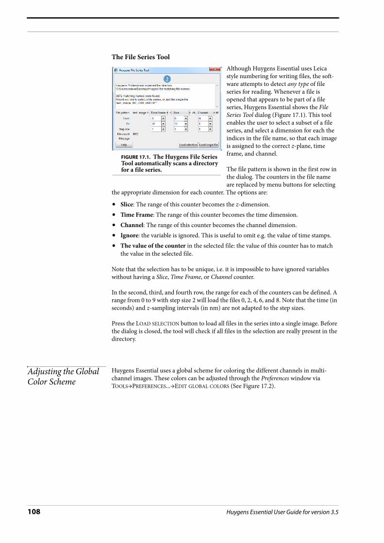
The File Series ToolAlthough Huygens Essential uses Leica style numbering for writing files, the soft-ware attempts to detect any type of file series for reading. Whenever a file is opened that appears to be part of a file series, Huygens Essential shows the File Series Tool dialog (Figure 17.1). This tool enables the user to select a subset of a file series, and select a dimension for each the indices in the file name, so that each image is assigned to the correct z-plane, time frame, and channel.

The file pattern is shown in the first row in the dialog. The counters in the file name are replaced by menu buttons for selecting

the appropriate dimension for each counter. The options are:

• Slice: The range of this counter becomes the z-dimension.• Time Frame: The range of this counter becomes the time dimension.• Channel: The range of this counter becomes the channel dimension.• Ignore: the variable is ignored. This is useful to omit e.g. the value of time stamps.• The value of the counter in the selected file: the value of this counter has to match

the value in the selected file.

Note that the selection has to be unique, i.e. it is impossible to have ignored variables without having a Slice, Time Frame, or Channel counter.

In the second, third, and fourth row, the range for each of the counters can be defined. A range from 0 to 9 with step size 2 will load the files 0, 2, 4, 6, and 8. Note that the time (in seconds) and z-sampling intervals (in nm) are not adapted to the step sizes.

Press the LOAD SELECTION button to load all files in the series into a single image. Before the dialog is closed, the tool will check if all files in the selection are really present in the directory.

Adjusting the Global Color Scheme

Huygens Essential uses a global scheme for coloring the different channels in multi-channel images. These colors can be adjusted through the Preferences window via TOOLS→PREFERENCES...→EDIT GLOBAL COLORS (See Figure 17.2).

FIGURE 17.1. The Huygens File Series Tool automatically scans a directory for a file series.


Hue Selector

Hue Selector The hue selector is a component that allows adjustment of the color range in which objects are displayed (See “The Surface Renderer” on page 41 and “The Colocalization Analyzer” on page 85). Objects belonging to different channels can be represented in dif-ferent hue ranges to make them clearly distinct. The gradual differences inside the selected range make independent objects distinguishable. Also a range can be collapsed to have all objects in a channel displayed with exactly the same color. In Huygens the hue selector does appear in two flavors.

Hue RangeThis selector allows the adjustment of a hue range. The objects on which this selector acts will get a color that lies within this range. The assignment of colors is based on the position of an object or on another parameter.

Hue Range and SaturationThis selector allows the adjustment of a single hue value and a satura-tion. The upper triangle defines the color, while the lower triangle sets the saturation for this color; left is white, right is fully saturated.

Image Statistics Right-click on a thumbnail image and select SHOW PARAMETERS from the pop-up menu. This window shows, besides the parameter settings, statistical information of the partic-ular image. Amongst them are the mean, sum, standard deviation, norm, and position of the center of mass.

FIGURE 17.2. The global color scheme can be modified through the Preferences window.


Setting the Coverslip Position

When there is a mismatch between the refractive index for which the microscope's objective is designed and the actual refractive index of the embedding medium, the shape of the point spread function (PSF) will be distorted due to spherical aberration (See “Refractive Index Mismatch” on page 101). As deeper layers in the specimen are imaged, moving away from the coverslip, this distortion will progressively worsen. To compute the spherical aberration it is necessary to know the distance from the coverslip. Because in many cases the coverslip position does not coincide with the first plane in the data, this position can be set in the microscopic parameter editor. To our knowledge none of the existing microscopic image files record the coverslip position in the meta data.

Next to direct numerical input, the cov-erslip position and imaging direction can be set using a visual editor (Figure 17.3), reachable from the parameter editor or from the Huygens Essential wizard by clicking the wrench button ( ).

Inverted MicroscopeThe editor shows the coverslip position and imaging direction relative to the data as read from the microscopic file. In an inverted microscope, with the objective physically below the speci-men it is likely that the first xy-plane in the data, corresponding with the lowest location in the xz maximum intensity projection (MIP) on the screen, corre-sponds with the xy-plane scanned clos-est to the objective. This situation is shown in REF TO FIG. However, since scan directions and data planes might

have been reordered, this match is not guaranteed. Fortunately, it is often easy to spot the flat side of the object where it adheres to the glass, so the orientation can be verified.

Upright MicroscopeIn an upright microscope, and a z-scan starting away from the coverslip, the first plane is also likely to be physically the lowest plane. In that case, the imaging direction should be set to downwards and the coverslip position in the top part of the xz MIP projection. However, if the scan started close to the coverslip while storing these first planes first in the data set, the MIP projection will show the data upside down. Consequently, the cov-erslip position will be in the lower part of the MIP, and the imaging direction is upward.

Slide PositionWhen the specimen is mounted on the coverslip, the distance from the object to the slide is probably in the range from 50 to100 μm, outside of the image. In this case, or in the case there is no slide, select Far away in the top-right selector.

FIGURE 17.3. The coverslip position editor showing an xy MIP of the data along they y-direction. The coverslip position can be adjusted by dragging the blue line. The imaging direction, here upwards, is indicated by the position of the objective relative to the data as shown. The z-position shown top-left in the image indicates the distance in μm of the coverslip to the first data plane.


Excitation Beam Overfill Factor

When the specimen is close to or mounted on the slide, select Close to object (). Drag the coverslip to its proper location. When this location is at some distance from the data it might be necessary to zoom out. The image can be dragged by holding down the right mouse button. In terms of imag-ing quality, when there is a refractive index mismatch between embedding medium and immersion medium, this is not an ideal situation since the light from and to the objective must travel hundreds of wavelengths through the embedding medium, possibly resulting in strong spherical aberration induced bloating of the PSF.

Excitation Beam Overfill Factor

In confocal microscopes, the entry pupil of the microscope objective is illuminated by a laser beam. Usually, laser beams have a Gaussian intensity profile2. As a result, the illu-mination intensity is not constant over the pupil but will decrease towards the edges. Lower edge intensities will lower the effective NA and therefore negatively affect resolu-tion. In most confocal microscopes this is remedied by using a beam width which is sig-nificantly larger than the entry pupil, at the cost of loss of excitation power. The ratio between the beam width and the pupil diameter is the excitation beam overfill factor (See Figure 17.5) and is typically in the range from 2 to 4.

FIGURE 17.4. The Coverslip editor with the slide position set to Close to object.

2.http://en.wikipedia.org/wiki/Gaussian_beam

-5.0 -2.5 0.0 2.5 5.00.00

0.25

0.50

0.75

1.00

Rela

tive

Beam

Inte

nsity

Relative Distance from Optical Axis

exp(-2(x/1)^2)exp(-2(x/2)^2)exp(-2(x/4)^2)

FIGURE 17.5. Lens entry pupil (red), beam profile with overfill factor 1 (blue), 2 (green), and 4(dark red). At overfill factor 1, the beam intensity is 14 % of the maximum, at overfill factor 2 the edge intensity is 61 % of the maximum.


The overfill factor can be set as a microscopic parameter in Huygens Essential, and is taken into account when computing the point spread function.

Brightfield Images Brightfield imaging is not a linear imaging process. In a linear imaging process the image formation can be described as the linear convolution of the object distribution and the point spread function, hence the name deconvolution for the reverse process. So in prin-ciple one cannot apply deconvolution based on linear imaging to non linear imaging modes like brightfield and reflection. One could state that the image formation in these cases is linear because it is governed by linear superposition of amplitudes. However, microscopes do not measure light amplitudes but rather intensities, i.e. the absolute squared values of the amplitudes. Taking the absolute square destroys all phase informa-tion one would need to effectively apply deconvolution. Fortunately, in the brightfield case the detected light is to a significant degree incoherent. Because in that case there are few phase relations the image formation is largely governed by the addition of intensities, especially if one is dealing with a high contrast image.

In practice one goes about deconvolving brightfield images by inverting them (using TOOLS→INVERT IMAGE image) and processing them further as incoherent fluorescence widefield images. The Tikhonov Miller algorithm was proven to work excellently for brightfield data. This algorithm is available in the Huygens Professional only. With the MLE algorithm one should watch out sharply for interference like patterns (periodic rings and fringes around objects) in the measured image. As a rule these become pro-nounced in low contrast images. After the deconvolution run a reverse to the original contrast setting is possible.

Support and Contact Information

Addresses and Phone Numbers

We are directly reachable by phone during office hours (CET) or by e-mail 24/7.

Distributors

A up-to-date list of distributors can be found on our web site3.

SVI Support Wiki

The SVI-wiki4 is a rapidly expanding public knowledge resource on 3D microscopy and deconvolution. Based on the WikiWikiWeb principle, it is open to contributions from

Mailing Address Scientific Volume Imaging B.V.Laapersveld 631213 VB HilversumThe Netherlands

Phone +31 35 6421626Fax +31 35 6837971E-mail [email protected]

URL http://www.svi.nl

3.http://www.svi.nl/distributors/



Support and Contact Information

every visitor. In addition it serves as a support medium for SVI customers and relations to discuss different aspects of the Huygens software.

This is a list of useful starting points in the SVI Support Wiki to learn more about the Huygens software and microscopical imaging in general:

• Information on the parameters describing the imaging conditions (sampling, numer-ical aperture, pinholes, etc.):http://support.svi.nl/wiki/MicroscopicParameters

• Information on the restoration parameters (signal to noise ratio, background, quality criteria, etc.) used by the deconvolution algorithms:http://support.svi.nl/wiki/RestorationParameters

• A step by step example on how to tune these parameters to achieve the desired resto-ration results:http://support.svi.nl/wiki/DeconvolutionProcedure

• Important issues regarding image acquisition and restoration (sampling, clipping, etc.):http://support.svi.nl/wiki/ImportantFactors

• Typical acquisition pitfalls (spherical aberration, undersampling, bleaching, etc.):http://support.svi.nl/wiki/AcquisitionPitfalls

• Information on recording beads to measure a PSF:http://support.svi.nl/wiki/RecordingBeads

• Tutorials and detailed information on using the different aspects of the Huygens soft-ware (restoration, visualization, analysis, programming, etc.):http://support.svi.nl/wiki/Tutorials

• Uploading images to SVI:http://support.svi.nl/wiki/SendImagesToSvi


Huygens Essential User Guide fo

Index

AAddress iv, 112Airy disk 97Analyze object 57Anchor 76Animation

frame count 35, 40, 44frame rate 35, 40, 44MIP 35Movie Maker 47SFP 40Surface Renderer 44

AVI files 50

BBackground 14, 88Backprojected

pinhole radius 10, 96pinhole spacing 10, 96

Base line 95Batch Processor 19Beads 90, 92Black level 14, 95Bleaching 103Bleaching correction 15Bounce 52Brick layout 15Bricks 93Brightfield images 112Brightness 27

CCenter scene 35, 44Channels 16Clipping 14, 102CMLE 15Colocalization 67, 85

coefficients 87map 87

Color mode 35, 40

Colors 27, 28, 108Compress 27Concurrent tasks 23Contact SVI 112Contrast 27Convert 10Correlation 67Coverslip position 10, 110Cropper 12csv file 63

DDeconvolution

templates 21wizard 9

Discard object 57Distiller 89Distributors 112Drift 17Dynamic range 95

EE-mail iv, 112Emission

transparency 39wavelength 11

Excitationfill factor 11, 111photon count 11transparency 39wavelength 11

Experiment preset 60, 77

FFax number iv, 112File

Formats 9Open 9Save 17Series 107

r version 3.5 115

116

Fill factor 11Filter Objects 79Freeware mode 4

GGamma 27Garbage volume 43, 56Geometrical distortion 101Global color scheme 108

Hhgst file 12hgsv file 35, 40, 44Histogram 13, 62

IImaging direction 10Installation 3

Linux 3Mac OS X 3path 6Uninstall 7Windows 3

Intensity profile 30Iso-surface 41Iteration mode 15Iterations 15

KKeyframes 48

LLeica numbering 107Lens refractive index 10License string 4, 105Linking 29Linux 3

MMac OS X 3Markers 30Maximum Intensity Projection 33Measure

Aspect Ratio 67Colocalization 67, 85Correlation 67Intensity profile 30Length 30, 65Principal Axis 65Sphericity 66

Medium refractive index 10Memory 7Microscope type 10Microscopic parameters 10MIP 33Mouse mode 57, 72Movie Maker 47Multi-channel images 16

NNumber of iterations 15

Numerical aperture 10Nyquist rate 95, 102

OObject Analyzer 53Object size 38Objective quality 10Overfill factor 111

PParameter templates 12Parameters 10Phone number iv, 112Photodamage 102Pinhole

radius 10, 96spacing 10, 96Spinning disk 98Square 97

PipeMode 74Render 42, 58, 78

Point spread function 89, 106Presets 50, 60, 77Principal axis 65Processor 7PSF 106

Asymmetric 101Distiller 89Experimental 104

QQuality factor 107Quality threshold 15

RRefractive index

Lens 10Medium 10Mismatch 101

Region of interest 70Render

MIP 33pipes 42, 58, 78quality 35, 40SFP 37size 35, 40, 44Surface 41

ROI 70

SSampling density 95Saturation 14Segmentation 55Select area 57Select object 57SFP 37Shape factor 97Signal to noise ratio 15, 93Slide position 110SNR 15, 93

Huygens Essential User Guide for version 3.5

Huygens Essential User Guide fo

Spherical aberration 101, 104, 110Sphericity 66Statistics 59, 109Storyboard 49Support 112Surface Renderer 41System ID 4, 106System requirements 7

TTable style 40Task 22Templates

Deconvolution 21Microscopic 12, 21Visualization 35, 40, 44

Threads per task 23Threshold 33, 38, 42, 55Time series 10Timeline 50Total internal reflection 102Transitions 49Transparency 43Transparency depth 44Twin Slicer 25

UUndersampling 102Uninstall 7Updates 5, 6

WWavelength

Emission 11Excitation 11

Windows 3Wizard 9, 89

r version 3.5 117

118
Huygens Essential User Guide for version 3.5

Huygens - Experimental Oncology Graduate Study

Documents

Transcript of Huygens - Experimental Oncology Graduate Study