HURRAY TR 080501

Scheduling Arbitrary-Deadline Sporadic Task Systems on Multiprocessors

Björn Andersson, Konstantinos Bletsas andSanjoy Baruah

www.hurray.isep.ipp.pt

Technical Report

HURRAY-TR-080501

Version: 0

Date: 09-09-2008

Technical Report HURRAY-TR-080501 Scheduling Arbitrary-Deadline Sporadic Task Systems on Multiprocessors

© IPP Hurray! Research Group www.hurray.isep.ipp.pt

1

Scheduling Arbitrary-Deadline Sporadic Task Systems on Multiprocessors Björn Andersson, Konstantinos Bletsas and Sanjoy Baruah

IPP-HURRAY!

Polytechnic Institute of Porto (ISEP-IPP)

Rua Dr. António Bernardino de Almeida, 431

4200-072 Porto

Portugal

Tel.: +351.22.8340509, Fax: +351.22.8340509

E-mail: [email protected], [email protected], [email protected]

http://www.hurray.isep.ipp.pt

Abstract A new algorithm is proposed for scheduling preemptiblearbitrary-deadline sporadic task systems upon multiprocessor platforms, with interprocessor migration permitted. This algorithmis based on a task-splitting approach --- while most tasks areentirely assigned to specific processors, a few tasks (fewer thanthe number of processors) may be split across two processors. This algorithm can be used for two distinct purposes: for actuallyscheduling specific sporadic task systems, and for feasibilityanalysis. Simulation-based evaluation indicates that this algorithm offers asignificant improvement on the ability to schedulearbitrary-deadline sporadic task systems as compared to thecontemporary state-of-art.With regard to feasibility analysis, the new algorithm is proved tooffer superior performance guarantees in comparison to prior feasibility tests.

Scheduling Arbitrary-Deadline Sporadic Tasks on Multiprocessors

Bjorn Andersson∗ Konstantinos Bletsas∗ Sanjoy Baruah†

Abstract

A new algorithm is proposed for scheduling preemptible arbitrary-deadline sporadic task systems upon multiprocessorplatforms, with interprocessor migration permitted. Thisalgorithm is based on a task-splitting approach — while mosttasks are entirely assigned to specific processors, a few tasks (fewer than the number of processors) may be split across twoprocessors. This algorithm can be used for two distinct purposes: for actually scheduling specific sporadic task systems,and for feasibility analysis. Simulation-based evaluation indicates that this algorithm offers a significant improvement on theability to schedule arbitrary-deadline sporadic task systems as compared to the contemporary state-of-art. With regard tofeasibility analysis, the new algorithm is proved to offer superior performance guarantees in comparison to prior feasibilitytests.

1 Introduction

Consider the problem of preemptively schedulingn sporadically arriving tasks onm identical processors. A taskτi isuniquely indexed in the range 1..n and a processor likewise in the range 1..m. A task τi generates a (potentially infinite)sequence of jobs. The arrival times of these jobs cannot be controlled by the scheduling algorithm and area priori unknown.We assume that the time between two successive jobs by the same taskτi is at leastTi. Every job byτi requires at mostCi time units of execution over the nextDi time units after its arrival. We assume thatTi, Di andCi are real numbers and0 ≤ Ci ≤ Di. A processor executes at most one job at a time and a job is not permitted to execute on multiple processorssimultaneously.

A task set can, depending on its deadlines, be categorized ashavingimplicit deadlines, constrained deadlinesor arbitrarydeadlines. A task set is said to be of implicit deadlines if∀i : Di = Ti. A task set is said to be of constrained deadlinesif ∀i : Di ≤ Ti. Otherwise, a task set is said to be of arbitrary deadlines. We consider the arbitrary-deadline model in thispaper. In this model, a job may arrive although the deadline of a previously released job of the same task has not yet expired.Because of this, there may be instants where two jobs of the same task are ready for execution. We require that two jobs ofthe same task are not permitted to execute simultaneously. With this requirement, it follows that if a taskτi hasCi > Ti thenit is impossible to schedule that task to meet deadlines. Forthis reason, we assumeCi ≤ Ti.

Algorithms for scheduling sporadic task systems on multiprocessors have traditionally been categorized aspartitionedor global. Global scheduling stores tasks which have arrived but not finished execution in one queue, shared by all proces-sors. At any moment, them highest-priority tasks among those are selected for execution on them processors. In contrast,partitioned scheduling algorithms partition the task set such that all tasks in a partition are assigned to the same processor.Tasks may not migrate from one processor to another. The multiprocessor scheduling problem is thus transformed to multipleuniprocessor scheduling problems. This simplifies scheduling and schedulability analysis as the wealth of results in unipro-cessor scheduling can be reused. Partitioned scheduling algorithms suffer from an inherent performance limitation inthat atask may fail to be assigned to any processor although the total available processing capacity across all processors is large.Global scheduling has the potential to rectify this performance limitation. In fact, there exist a family of algorithmscalledpfair [8, 1] which are able to schedule tasks to meet deadlines evenwhen up to 100% of the processing capacity is requested.

∗IPP-HURRAY! Research Group, Polytechnic Institute of Porto (ISEP-IPP), Rua Dr. Antonio Bernardino de Almeida 431, 4200-072 Porto, Portugal –[email protected], [email protected]

†Department of Computer Science, University of North Carolina, Chapel Hill, NC 27599, USA – [email protected]

Unfortunately, these algorithms have two drawbacks; they are only designed for implicit deadlines. Also, all task parametersmust be multiples of a time quantum and in every quantum a new task is selected for execution. Preemption counts can thusbe high [11].

Recent advances in the real-time scheduling theory have however made a new class [2, 12, 10, 5, 3] of algorithms availablewith the purpose of offering the best of both global scheduling and partitioning. Tasks are assigned to processors in a waysimilar to partitioning but if the task cannot be assigned toa processor then the task is “split” into two pieces and thesetwo“pieces” are scheduled by a uniprocessor scheduling algorithm on each processor. The splitting approach uses dispatchers oneach processor which ensure that a split task never executeson two processors simultaneously.

The task splitting approach has been successfully, and widely, used in scheduling implicit-deadline systems. Andersonet al. [2] designed an algorithm which can miss deadlines butit offers the guarantee that even at high processor utilization,the finishing time is not too much later than its deadline and this amount is low and bounded. Kato et al. [12] designed analgorithm aiming to meet deadlines and it performed well in simulations. The task splitting approach has also been used[10, 5, 3] to design algorithms for both periodic and sporadic tasks such that if at most a certain fraction (greater than 50%)of the total processing capacity is requested then all deadlines are met. Despite these successes of the task splitting approachfor scheduling implicit-deadline tasks, task splitting has not been used for scheduling arbitrary-deadline sporadictasks. Infact, we are not aware of any previous work (with task splitting or some other approach) that aims for offering pre-run-timeguarantees in scheduling arbitrary-deadline tasks on a multiprocessor with performance better than what partitioning schemescan offer.

Our algorithm. In this paper, we present a new algorithm for scheduling arbitrary-deadline sporadic tasks on a multi-processor that is based on task splitting. We call this algorithm EDF-SS(DTMIN/δ), the name denotingEarliest-Deadline-First scheduling of non-split tasks withSplit tasks scheduled inSlots of durationDTMIN/δ. The symbol DTMIN denotesmin(D1,D2,. . . ,Dn,T1,T2,. . .,Tn), andδ is an integer parameter (≥1) that is selected by the designer. Thus for a given tasksystem the value assigned toδ determines the scheduling slot size used. The smaller this slot size, the more frequently splittasks migrate between the processors that they utilize. As we will see, by choosing different values forδ the designer is ableto trade offschedulability– the likelihood of a system being guaranteed schedulable – for a lower number of preemptions.More specifically, we will derive (Theorem 2) an upper bound on the number of preemptions per job in a schedule as afunction ofδ and the task parameters: the smaller the value ofδ, the fewer the number of preemptions. We also quantify (inSection 2.3) the amount by which the execution requirementsof jobs are “inflated” by our scheduling algorithm in order toguarantee that all deadlines are met: we will see that the larger the value ofδ, the smaller the amount of such inflation. Thusa larger value ofδ makes it more likely that a particular task system will be determined to be schedulable, but the generatedschedule is likely to have a larger number of preemptions.

Using our algorithm. By choosing an appropriate value ofδ, we can use our scheduling algorithm in two different ways.First it can be used by a designer toschedule a specific task set. For such a use, the run-time dispatching overhead isimportant. Our algorithm uses no global data-structures and is appropriate for that purpose. It is also important to maintaina low number of preemptions and hence the value ofδ should not be too large. For example choosingδ such that 1≤δ ≤ 4 seems reasonable. Baker [6] has conducted simulation experiments of randomly generated task sets of previouslyknown algorithms for arbitrary-deadline sporadic multiprocessor scheduling and evaluated them for the context wherepre-run-time guarantees are needed. Baker observed that generally speaking, partitioned algorithms tend to perform better thanglobal scheduling algorithms perhaps because partitionedscheduling algorithms are based on uniprocessor schedulabilitytests whereas currently known global schedulability teststend to be very pessimistic. The partitioning-based algorithm EDF-FFD [6] was found to be the champion among all algorithms studied. We compare our new algorithm EDF-SS(DTMIN/δ)with EDF-FFD in simulation experiments, with the same setupas Baker and we find that for everyδ ≥ 1, EDF-SS(DTMIN/δ)offers a significant performance improvement.

A second use of our schedulability algorithm is infeasibility analysis— determining whether a given task system can bescheduled by a hypothetical optimal algorithm to always meet all deadlines. Currently no exact (necessary and sufficient)algorithms are known for performing feasibility analysis of arbitrary deadline sporadic task systems. In fact, all currentfeasibility tests are based on actually using a specific scheduling algorithm and performing schedulability analysis for it. Asstated above, Baker [6] has observed that partitioning-based algorithms tend to perform better than global ones; by extendinga previously-proposed partitioning-based scheduling algorithm [7] to allow for task-splitting, our algorithm, withδ → ∞,yields a sufficient feasibility test that is superior to previously-proposed sufficient tests.

(a) The reserves on processors for the split taskτ2. (b) We require that a job from a split task finishes its execution at a mo-ment before its deadline.

Figure 1. How to perform run-time dispatching of tasks that a re assigned to two processors.

Organization. The remainder of this paper is organized as follows. Section2 presents the theoretical basis of our newalgorithm. Section 3 presents the new algorithm itself, andderives some of its properties while Section 4 discusses itsusein feasibility testing. Section 5 presents the performanceof the new algorithm obtained by running simulation experiments.Section 6 gives conclusions.

2 Conceptual foundations

Before describing the new algorithm, it is beneficial to get acquainted with the ideas behind its design and also certainconcepts and results that will be used. Section 2.1 explainshow task splitting is performed. Section 2.2 presents a dispatcherfor use with task splitting. Section 2.3 performs dimensioning of the reserves used for execution of split tasks. Section 2.4derives the amount of execution of split tasks. Section 2.5 presents a new schedulability analysis for real-time scheduling ona single processor.

2.1 Task Splitting

As mentioned in Section 1, partitioned scheduling offers the advantage that results from the vast body of uniprocessorscheduling theory can be reused to schedule tasks on a multiprocessor. The disadvantage of partitioned scheduling is alsowell-known: as tasks get assigned to processors, the remaining available capacity gets fragmented among the processors;it may then so happen that no individual fragment is large enough to accommodate an additional task (although the sum ofthese fragments would be sufficient for the additional task). Task splittingcircumvents this problem by permitting that a taskbe split across multiple processors. And in fact this idea has been used by several researchers [2, 12, 10, 5, 3] for schedulingsporadic or periodic tasks with implicit deadlines. In thiswork, we apply task-splitting to scheduling sporadic taskswitharbitrary deadlines, by allowing an individual task to be split between two processors. Our approach is similar to previouswork for implicit-deadline systems [3] but differs mainly (i) in the task assignment/splitting scheme used and (ii) in that,instead of a utilization-based schedulability test, a demand-based test is used, applicable to arbitrary-deadline systems.

Recall that our task model mandates that each task may be executing on at most one processor at each instant in time. Tasksplitting must therefore address two important challenges(i) create a dispatching algorithm for ensuring that two pieces of atask do not execute simultaneously and (ii) design a schedulability test for the dispatching algorithm. (Observe that becauseof (i), there is no need for the source code or the binary corresponding to a task to be restructured.)

2.2 Dispatching

Figure 1(a) provides further details on run-time dispatching. We subdivide the time into time slots of durationS=DTMIN/δ.The time slots on any two different processors are synchronized in time. On processorp, the beginning of a time slot is re-served for executing a split taskτi shared with processorp-1; let x[p] denote the duration of this reserve. Analogously, thefinal part of a time slot on processorp is reserved for executing a split task shared with processorp+1; let z[p] denote theduration of this reserve.

Figure 2. An example showing that at certain instants, a rese rve may be unused.

The dispatching is simple. If processorp is in a reserve at timet and if the split task assigned that reserve has unfinishedexecution then the split task is executed in that reserve on processorp at timet. Otherwise, the non-split task, assigned toprocessorp, with the earliest deadline is selected for execution.

2.3 Dimensioning of the Reserves

A task that is split over processorsp − 1 andp executes during the reservesz[p-1] andx[p]. For δ < ∞, we will seethat the total amount of these reserves must exceed the splittask’s execution requirement in order to guarantee that thesplittask meets its deadline. We now derive “safe” values for these reserves, which will ensure that all jobs of the split tasksareguaranteed to meet their deadlines. In deriving these values, the objective is to minimize the inflation – the amount by whichthe reserves exceed the execution requirement.

In order to meet deadlines we need to ensure that for each jobJi,k of taskτi it holds that wheneverJi,k arrives, it completesCi time units at mostDi time units after its arrival. For split tasks, we have chosento impose an even stronger requirement;we require that within

⌊

min(Di, Ti)

S

⌋

· S (1)

time units after its arrival, the jobJi,k should completeCi time units. Figure 1(b) illustrates this. Equation 1 implies thatdeadlines of split tasks are met and it also implies that a split task finishes before it arrives again. Observe that the durationin Equation 1 is an integer multiple ofS. We know that for any time interval of durationS (which does not necessarily startat a slot boundary), it holds that the amount of execution available (in reserves) for a split taskτi is x[p]+z[p-1]. Thereforewe obtain that during a time interval of duration given by Equation 1, the amount of execution available for the split taskτi

assigned to processorp and processorp-1 is exactly⌊

min(Di, Ti)

S

⌋

· (x[p] + z[p − 1]) (2)

In order to meet deadlines we should selectx[p] and z[p-1] such that the expression in Equation 2 is at leastCi. We areinterested also in using “small reserves” and for this reason we choosex[p] andz[p-1] such that it is equal toCi. Hence weselectx[p] andz[p-1] such that

x[p] + z[p− 1] =Ci

⌊min(Di,Ti)S

⌋(3)

Clearly, the choice by Equation 3, gives us that whenever a job of a split taskτi is released, it finishes within at most⌊min(Di, Ti)/S⌋ · S time units, as desired (see Equation 1 above). A property which we will find useful in the next sectionthat follows from Equation 3 is that if a job released by a split taskτi executes forCi time units then it executes exactly

⌊

min(Di, Ti)

S

⌋

· x[p] (4)

time units on processorp and⌊

min(Di, Ti)

S

⌋

· z[p − 1] (5)

time units on processorp-1.

2.4 Execution by Split Tasks

In order to perform schedulability analysis (in Section 2.5below), we must obtain an upper bound on the amount ofexecution that the split tasks perform on a processorp during any time interval of durationL. We now derive such an upperbound. This upper bound is given in Equation 8; the reader maywish to skip its derivation (i.e., the remainder of Section 2.4)at a first reading and return to it later.

It is easy to see that if jobs of a split task during this time interval execute for less than their maximum execution time thenwe can obtain another scenario with no less execution of split tasks on processorp duringL, by letting jobs execute by theirmaximum amount1. Hence, we will assume that all jobs from split tasks executefor their maximum execution time. Let usdefineslotexecas:

slotexec(t, r) =

⌊

t

S

⌋

· r + min(t −

⌊

t

S

⌋

· S, r) (6)

Slotexecgives us an upper bound on the amount of execution performed by a split task in a time interval of durationt,assuming that it executes in all of its reserves and assumingthat each reserve assigned to that task has the durationr. Thisbound can be used to find an upper bound on the amount of time that split tasks execute on processorp.

But consider the example in Figure 2. It shows a taskτ2 split between processors 2 and 1. The task hasT2 = 5 · SandD2 = 4.2 · S. For the scenario in Figure 2, it follows that during [4.4 · S,5.3 · S), the reserve on processor 2 for taskτ2 is unused. For this reason, we need to calculate an upper bound on the amount of execution of split tasks by taking theparameters of the split tasks into account. We will do so now.

Let τhi,p denote the task that is split between processorp and processorp-1. Analogously, letτlo,p denote the task that issplit between processorp and processorp+1.

With this definitions, one can show (see [4, Appendix A]) thatthe amount of execution of taskτhi,p on processorp duringa time interval of durationL is at most:

⌊

L + S − x[p]

Thi,p

⌋

· Chi,p ·x[p]

x[p] + z[p− 1]+

slotexec(min(L + S − x[p] −

⌊

L + S − x[p]

Thi,p

⌋

· Thi,p,

⌊

min(Dhi,p, Thi,p)

S

⌋

· S), x[p])

(7)

Intuitively, Equation 7 can be understood as follows. When finding the amount of execution ofτhi,p duringL, it is actuallynecessary to consider arrivals ofτhi,p duringL + S − x[p] because the taskτhi,p may arriveS − x[p] time units before the

beginning of the interval of durationL. The time interval of durationL + S − x[p] can be subdivided into⌊

L+S−x[p]Thi,p

⌋

time

intervals each one of durationThi,p and one time interval of duration

L + S − x[p] −⌊

L+S−x[p]Thi,p

⌋

· Thi,p.

Applying the reasoning of Equation 7 toτlo,p and adding them together gives us that the amount of execution of split taskson processorp during a time interval of durationL is at most:

1For split taskτi with Di ≤ Ti it is easy to see this because increasing the execution time of a job of such a task does not affect the scheduling of anyother jobs of split taskτi. For the case of a taskτi with Di > Ti it may not be so easy to see because one may think that two jobs of a task may be activesimultaneously and then increasing the execution time of the former job may change the starting time of execution of the latter job. This cannot happenthough because of our choice expressed in Equation 3.

⌊

L + S − x[p]

Thi,p

⌋

· Chi,p ·x[p]

x[p] + z[p− 1]+


⌊

L + S − x[p]

Thi,p

⌋

· Thi,p,

⌊

min(Dhi,p, Thi,p)

S

⌋

· S), x[p]) +

⌊

L + S − z[p]

Tlo,p

⌋

· Clo,p ·z[p]

x[p + 1] + z[p]+

slotexec(min(L + S − z[p]−

⌊

L + S − z[p]

Tlo,p

⌋

· Tlo,p,

⌊

min(Dlo,p, Tlo,p)

S

⌋

· S), z[p])

(8)

2.5 Schedulability Analysis

The processor demand [9] is a well-known concept for feasibility testing on a single processor. Intuitively, the processordemand represents the amount of execution that must necessarily be given to a task in order to meet its deadline. Theprocessor demand of a taskτj in a time interval of durationL is the maximum amount of execution of jobs released byτj such that these jobs (i) arrive no earlier than the beginningof the time interval and (ii) have deadlines no later than thefinishing of the time interval. Letdbf(τj,L) denote the processor demand of taskτj over a time interval of durationL. It isknown [9] that:

dbf(τj , L) = max(0,

⌊

L − Dj

Tj

⌋

+ 1) · Cj (9)

The processor demand of a task set is defined analogously. Letdbf(τ ,L) denote the processor demand of the task setτ ofa time interval of durationL. It is known that:

dbf(τ, L) =∑

τj∈τ

max(0,

⌊

L − Dj

Tj

⌋

+ 1) · Cj (10)

One can show [9] that for EDF [13] scheduling on a single processor, it holds that all deadlines for tasks inτ are metif and only if ∀L > 0: dbf(τj ,L) ≤ L. In fact, we only need to check this condition for the values of L where there is anon-negative integerk and a taskτi such thatL=k · Ti + Di andL does not exceed 2· lcm(T1,T2,. . .,Tn). This conditioncan be used as a schedulability test for partitioned scheduling where EDF is used on each processor. Recall however that thetask splitting approach we use requires that split tasks areexecuted in special time intervals in the time slots and hence a newschedulability analysis must be developed. We know that if the processor demand of the non-split tasks during a time intervalL (expressed by Equation 10) plus the amount of execution of the split tasks (expressed by Equation 8) does not exceedLthen all deadlines are met. Let us define:

f(L) =∑

τj∈τp

max(0,

⌊

L − Dj

Tj

⌋

+ 1) · Cj +

min(L,

⌊

L + S − x[p]

Thi,p

⌋

· Chi,p ·x[p]

x[p] + z[p− 1]+


⌊

L + S − x[p]

Thi,p

⌋

· Thi,p,

⌊

min(Dhi,p, Thi,p)

S

⌋

· S), x[p]) +

⌊

L + S − z[p]

Tlo,p

⌋

· Clo,p ·z[p]

x[p + 1] + z[p]+

slotexec(min(L + S − z[p]−

⌊

L + S − z[p]

Tlo,p

⌋

· Tlo,p,

⌊

min(Dlo,p, Tlo,p)

S

⌋

· S), z[p]) )

(11)

Clearly this gives us that

if

∀L, L = k · Ti + Di, L ≤ 2 · lcm(T1, T2, . . . , Tn) :

f(L) ≤ L

then all deadlines are met (12)

2.6 Faster Schedulability Analysis

Consider the schedulability analysis in Equation 12. It canbe seen that a large number of values ofL must be explored.Our task splitting approach requires that several such schedulability tests are performed and consequently we are interestedin creating a faster schedulability analysis. Let us defineLlim as follows:

Llim =

(∑

τj∈τp Cj) + 2 · S + Thi,p + Tlo,p

1 − ((∑

τj∈τp

Cj

Tj) +

Chi,p

Thi,p· x[p]

x[p]+z[p−1] +Clo,p

Tlo,p· z[p]

x[p+1]+z[p] )

(13)

Let us consider the case that the denominator of the right-hand side Equation 13 is positive. LetDMAX denotemax(D1, D2, ..., Dn).Then it holds (see Appendix B in Technical Report HURRAY-TR-080501 available at http://www.hurray.isep.ipp.pt) thatf(L) ≤ L for all L≥Llim. This idea was known for pure EDF scheduling on a uniprocessor [9] but now we have transferredthe result to a uniprocessor with reserves. Formally, this is stated as follows:

if

the denominator of the right − hand side of

Equation 13 is positive

and

∀L, L = k · Ti + Di,

L < min(2 · lcm(T1, T2, . . . , Tn), max(DMAX, Llim)) :

f(L) ≤ L


2.7 Design Consideration of Task Assignment

Previous work on task splitting [3] for implicit-deadline tasks was based on next-fit bin-packing. Unfortunately, suchusefor scheduling arbitrary-deadline tasks can lead to poor performance, as shown in Example 1.

Example 1. Consider three tasks and two processors. The tasks are characterized asT1=L2,D1=L,C1=L · (2/3+ǫ),T2=L2,D2=L, C2=L · (2/3+ǫ), T3=L2,D3=1, C3=2/3+ǫ. Let L denote a positive number much larger than one. Andlet ǫ denote a positive number much smaller than one. Note thatτ1 andτ2 are identical and they have largeDi. The taskτ3

has smallDi however.A next-fit bin-packing algorithm with task splitting would start consideringτ1 and it would be assigned to processor 1.

The next task to be considered would beτ2 and it would be attempted to be assigned to processor 1 but theschedulability testwill fails so the task will be split between processor 1 and processor 2. The capacity of processor 1 assigned toτ2 will be1/3-ǫ and the capacity assigned toτ2 will be 1/3+2ǫ. The next task to be considered would beτ3 and it would be consideredfor processor 2. Unfortunately, it cannot be assigned there. The reason is that during a time window of duration 1, thereserves forτ2 will be busy by execution ofτ2 and this does not give enough time toτ3 to execute and hence it would missa deadline. Intuitively, this can be understood as priorityinversion, whereτ3 is ready for execution and it has the shortestdeadline but stillτ2 executes andτ2 has a much longer deadline.

It can be seen, from Example 1, that it is advantageous to assign tasks such that tasks with large deadlines are non-splitand tasks with short deadlines are split. A bin-packing algorithm based on first-fit (boosted with a task splitting approach inthe end) might achieve that. But unfortunately, another performance penalty would arise, as shown in Example 2.

Example 2. Considerm+1 tasks andm processors. The tasks are characterized asTi=1,Di=1,Ci=2/3+ǫ. Let ǫ denote apositive number much smaller than one.

A first-fit bin-packing algorithm with task splitting would start by assigning one task to each processor. Then it wouldconsider taskτm+1 and find that it cannot be assigned to any processor. Therefore splitting is attempted; the task is splitinto two pieces but even in this way, it cannot be assigned to two processors. It is necessary to split the task into three ormore pieces in order to meet deadlines. Such splitting makesrun-time dispatching non-trivial; we note in particular that theapproach sketched on Figure 1 cannot be used.

We have seen, from Example 1 and Example 2, that (i) a processor should be “filled” before new processors are consideredand (ii) tasks that are split should preferably have a smallDi. This can be achieved as follows.

Initialize a variablep to one; it denotes the processor under consideration. For whichever processorp is in consideration,all tasks which are not yet assigned are scanned in order of decreasing deadline. If a task can be assigned (according to aschedulability test) to processorp then it is assigned there; if not, we consider if the next taskcan be assigned to processorp,subject to assignments already made (and so on).

After the scanning of all tasks has finished, it holds that of all the tasks that have still not been assigned to any processor,none can be assigned to processorp, subject to assignments already made. At this point, so as toutilize whatever capacity isstill remaining on processorp, we thus have to “split” one of those tasks and assign a piece of it to the processor. We selectfor this purpose, among all tasks not yet assigned assigned,the task with the smallestDi. It is split and assigned to processorsp andp + 1, such that as much execution as possible is assigned to processorp.

After that, the variablep is incremented by one and the procedure is repeated. Note that in this way, we obtain the twoproperties (i) and (ii) above and we can therefore expect good performance.

1. for each processor pdo2. x[p] := 03. z[p] := 04. τ [p] := ∅6. end for7. for each processor p with index p< m do8. sharedtask[p] := NULL9. end for

10. p := 111. unassigned :=τ12. while unassigned6= ∅ do13. for each taskτi ∈ unassigned, considered in descending

order ofDi do14. τ [p] := τ [p] ∪ { τi }15. if the test Equation 14 succeeds for processorp

and x[p]+z[p]≤S then16. unassigned := unassigned\ { τi }17. elseτ [p] := τ [p] \ { τi } end if18. end for19. if unassigned6= ∅ then20. if p ≤ m-1 then21. i := index of the task in unassigned with leastDi

22. sumreserve := right-hand side of Equation 323. if sumreserve> S then24. p := p + 125. else26. p := p + 127. assign values tox[p] andz[p-1] such thatz[p-1] is

maximized and the test Equation 14 succeeds forp-1and x[p-1]+z[p-1]≤ S and Equation 3 is true forp

28. sharedtask[p-1] :=τi

29. unassigned := unassigned\ { τi }30. end if31. elsedeclare FAILUREend if32. end if33. end while34. declare SUCCESS

Figure 3. An algorithm for assigning tasks to processors (an d performing splitting if needed).

3 The New Scheduling Algorithm

Let us now specify detailed pseudo-code for the new scheduling algorithm. The scheduling algorithm is comprised of twoalgorithms (i) one algorithm for assigning (and splitting if needed) tasks to processor and (ii) an algorithm for dispatchingthe tasks.

Figure 3 shows the algorithm for assigning tasks to processors. The main idea is to assign as many tasks as possible tothe current processorp. The lines 13-18 do that. The tasks are considered for assignment in the order largest-Di-first andthe decision on whether a task can be assigned to processorp is made based on whether Equation 14 can guarantee thisassignment. Once no additional task can be assigned to processorp, the unassigned task with the leastDi is selected and itis split between processorp and processorp+1. The lines 26-29 do that. The splitting is done such that asmuch as possibleof the currently considered task is assigned to processorp and as little as possible is assigned to processorp+1. Clearly, thisleaves as much room as possible on processorp+1 for other tasks. Equation 14 is used for this splitting.

A variablesumreserve is calculated (on line 22). It represents the sum of the reserve of the split taskτi on processorpand the reserve of the split taskτi on processorp+1. In order to ensure that the split taskτi does not execute on two processorssimultaneously, we comparesumreserve to S, the slot size. Ifsumreserve is greater then splitting is not possible andthe algorithm continues without splitting that task. Ifsumreserve does not exceedS then splitting is performed. Asalready mentioned, this splitting is performed on lines 26-29.

Line 27 states that a maximization problem should be solved.Note that the right-hand side of Equation 11 is non-decreasing with increasingz[p-1] and hence it can be solved easily.2

Figure 4 shows the algorithm for dispatching. It computes a time t0 which is the beginning of the time slot and a timet1 which is the end of the time slot. Based on that, it computestimea andtimeb which denote the end and the beginningrespectively of the two reservations.

We will now present the correctness of the algorithm in Figure 4 and Figure 5. We will also prove a bound on the numberof preemptions. In addition, we present equations for the case whereδ → ∞.

Theorem 1. If tasks are assigned according to the algorithm in Figure 3 and it declares SUCCESS and the algorithm inFigure 4 dispatches tasks at run-time then all deadlines aremet.

Proof. It follows from the schedulability analysis in Section 2.5 and Section 2.6.

Let us now state a bound on the number of preemptions.

Theorem 2. Assume that tasks are assigned according to the algorithm inFigure 3 and it declares SUCCESS and thealgorithm in Figure 4 dispatches tasks at run-time. Letnpreempt(t,p) denote an upper bound on the number of preemptionsgenerated on processorp in a time interval of durationt. Letτhi,p denote the task that is split between processorsp-1 andp.Analogously, letτlo,p denote the task that is split between processorsp+1 andp. LetS denote the size of the time slots. Letjobs(t, p) denote the maximum number of jobs that are released during a time interval of durationt from either (i) non-splittasks assigned to processorp or (ii) the task split between processorp-1 andp or (iii) the task split between processorp+1andp. We then have that:

npreempt(t, p) = jobs(t, p) + 2 +

min(⌈

tS

⌉

, activeslots(t, p)) · 3 (15)

where

activeslots(t, p) =⌈

tThi,p

⌉

·⌈

min(Dhi,p,Thi,p)S

⌉

+⌈

tTlo,p

⌉

·⌈

min(Dlo,p,Tlo,p)S

⌉

(16)

2A solution is as follows. LetLB denote a lower bound onz[p-1] and letUB denote an upper bound onz[p-1]. We know that one choice isLB = 0andUB = sumreserve so we start with that. Letmiddle denote (LB+UB)/2. We tryz[p-1]:=middle andx[p]:=sumreserve-middle and apply theschedulability test. If it succeeds then we setLB := middle otherwiseUB := middle. We repeat this procedure untilLB andUB are close enough (10iterations tend to be sufficiently good) and then computez[p-1]:=LB andx[p]:=sumreserve-LB.

1. when booting2. if another processor q has already performeddo

”‘when booting”’ then3. tstart[p] := tstart[q]4. else5. tstart[p] := any value6. end if7. lo active[p] := false8. hi active[p] := false9. end when booting

10. when a job released from a task split between processorprocessorp-1 andp arrivesdo

11. hi active[p] := true12. settimer again( p)13. dispatch(p)14. end when

15. when a job released from a task split between processorprocessorp+1 andp arrivesdo

16. lo active[p] := true17. settimer again( p)18. dispatch(p)19. end when

20. when a job released from a task split between processorprocessorp-1 andp finishesdo

21. hi active[p] := false22. settimer again( p)23. dispatch(p)24. end when

25. when a job released from a task split between processorprocessorp+1 andp finishesdo

26. lo active[p] := false27. settimer again( p)28. dispatch(p)29. end when

30. procedure set timer again( p : integer)is31. if lo active[p]=trueor hi active[p]=truethen32. t := readtime33. t0 := tstart +⌊ (t-tstart[p])/S⌋ · S34. t1 := tstart +⌊ (t-tstart[p])/S⌋ · S + S35. timea := t0 + x36. timeb := t1 - y37. end if38. end procedure

39. procedure dispatch( p : integer)is40. selected := NULL41. t := readtime42. if hi active[p]and t0 ≤ t < timeathen43. selected := task that is split between processor p-1

and processor p44. end if45. if lo active[p]and timeb≤ t < t1 then46. selected := task that is split between processor p

and processor p+147. end if48. if selected=NULLand there is a non-split task assigned48. to processor p that is readythen49. selected := the non-split task assigned to50. processor p with the earliest deadline50. end if51. end procedure

Figure 4. An algorithm for dispatching tasks.

Proof. Note that a preemption can only occur when either (i) a job arrives or (ii) a reserve begins or ends. The number ofpreemptions due to job arrivals is clearly at mostjobs(t, p). If we consider a time interval [t,t+S) then it holds that therecan be at most three preemptions caused by the beginning or ending of reserves. We can therefore subdivide a time intervalof durationL into time intervals of durationS, each with at most three time preemptions caused by the beginning or endingof reserves. And then add two preemptions because of the beginning and ending of the time interval of durationL. Thisreasoning gives us the theorem.

Consider now the problem of feasibility test of a task set, that is to decide if it is possible to schedule the task set. For sucha use, we recommend the use ofδ → ∞ with our algorithm. Let us introduce the following auxiliary variables:

xf [p] =x[p]

S(17)

and

zf [p] =z[p]

S(18)

Applying δ → ∞, Equation 17, Equation 18 and Equation 6 on Equation 3, Equation 11, Equation 13 and Equation 14yields that:

xf [p] + zf [p − 1] =Ci

min(Di, Ti)(19)

and

g(L) =∑

τj∈τp

max(0,

⌊

L − Dj

Tj

⌋

+ 1) · Cj +

min(L,

⌊

L

Thi,p

⌋

· Chi,p ·xf [p]

xf [p] + zf [p− 1]+

min(L −

⌊

L

Thi,p

⌋

· Thi,p, min(Dhi,p, Thi,p)) · xf [p] +

⌊

L

Tlo,p

⌋

· Clo,p ·zf [p]

xf [p + 1] + zf [p]+

min(L −

⌊

L

Tlo,p

⌋

· Tlo,p, min(Dlo,p, Tlo,p)) · zf [p] ) (20)

and

LGlim =

(∑

τj∈τp Cj) + Thi,p + Tlo,p

1 − ((∑

τj∈τp

Cj

Tj) +

Chi,p

Thi,p· x[p]


Tlo,p· z[p]

x[p+1]+z[p])

(21)

and

1. for each processor pdo2. xf[p] := 03. zf[p] := 04. τ [p] := ∅6. end for7. for each processor p with index p< m do8. sharedtask[p] := NULL9. end for

10. p := 111. unassigned :=τ12. while unassigned6= ∅ do13. for each taskτi ∈ unassigned, considered in descending

order ofDi do14. τ [p] := τ [p] ∪ { τi }15. if the test Equation 22 succeeds for processorp

and xf [p]+zf [p]≤1 then16. unassigned := unassigned\ { τi }17. elseτ [p] := τ [p] \ { τi } end if20. end for21. if unassigned6= ∅ then22. if p ≤ m-1 then23. i := index of the task in unassigned with leastDi

24. p := p + 125. assign values toxf [p] andzf [p-1] such thatzf [p-1] is

maximized and the test Equation 22 succeeds forprocessorp-1 andxf [p-1]+zf [p-1] ≤ 1 andEquation 19 is true forp

26. sharedtask[p-1] :=τi

27. unassigned := unassigned\ { τi }28. elsedeclare FAILUREend if29. end if30. end while31. declare SUCCESS

Figure 5. A feasibility test

if

the denominator of the right− hand side of


and

∀L, L = k · Ti + Di,

L < min(2 · lcm(T1, T2, . . . , Tn), max(DMAX, LGlim)) :

g(L) ≤ L

then all deadlines are met

(22)

Based on these equations we have a feasibility test as expressed by Figure 5.

4 Feasibility testing

A sporadic task system is said to befeasibleupon a specified platform if every possible sequence of jobs that can be legallygenerated by the task system can be scheduled upon the platform to meet all deadlines. Exact (necessary and sufficient) testsare known for determining feasibility for sporadic task systems upon preemptive uniprocessors [9]. For global schedulingupon preemptive multiprocessors, however, no exact (or particularly good sufficient) feasibility tests are known; obtainingsuch feasibility tests is currently one of the most important open problems in multiprocessor real-time scheduling theory.In particular, it would be useful to have feasibility tests that both perform well in practice (as determined by extensive

simulations) andare able to provide concrete quantitative performance guarantees. The kind of quantitative performanceguarantee we will look to provide is the processor speedup factor.

Definition 1 (Processor speedup factor). A feasibility test is said to have a processor speedup factors if any task systemdeemed to not be feasible upon a particular platform by the test is guaranteed to actually not be feasible upon a platform inwhich each processor is1/s times as fast.

A sufficient feasibility test that may perform arbitrarily poorly has a processor speedup factor of infinity, while an exactfeasibility test has a processor speedup factor of 1. Thus, the processor speedup factor of a sufficient feasibility testmaybe considered to be a quantitative measure of the amount by which the test is removed from being exact — the smaller theprocessor speedup factor, the closer to being an exact test and hence the better the test.

As stated in Section 1, current sufficient feasibility testsfor sporadic task systems adopt the approach of performingschedulability analysis of a specific scheduling algorithm(since any schedulable task system is trivially feasible).Baker [6]has experimentally evaluated the schedulability tests fora large number of scheduling algorithms, and observed that partitioning-based schedulability tests tend to perform better than global ones. Our approach in this section is to take a partitioningalgorithm that is able to make quantitative performance guarantees — the one proposed in [7] — and obtain a sufficientglobal feasibility test, which we call FEAS-SS, by extending it to incorporate task splitting. We will show that FEAS-SSisstrictly superior to the test in [7] (in the sense that it is able to demonstrate feasibility for all task systems determined to beschedulable by the test of [7] while there are task systems determined to be feasible by FEAS-SS that the test of [7] will notdetermine to be schedulable) — hence, FEAS-SS tends to perform better in practice than the schedulability test of [7]. Atthe same time, since FEAS-SS dominates the schedulability test of [7] it is able to make the same quantitative performanceguarantee as the test in [7].

The quantitative performance guarantee made by the schedulability test in [7] is as follows:

Theorem 3 (From [7]). If an arbitrary sporadic task system is feasible onm identical processors each of a particularcomputing capacity, then the scheduling algorithm in [7] successfully partitions this system upon a platform comprised ofmprocessors that are each(4 − 2

m) times as fast.

The scheduling algorithm in [7] has a run-time computational complexity of O(n2) wheren is the number of tasks;Theorem 3 therefore yields a polynomial-time (anO(n2)) sufficient feasibility test.

The partitioning algorithm of [7] considers tasks in non-decreasing order of relative deadline parameter, attemptingtoaccommodate each task onto any processor upon which it “fits”according to a polynomial-time testable condition (see [7]for details). The algorithm succeeds if all tasks are assigned to processors, and returns failure if it fails to assign some task.

FEAS-SS extends the partitioning algorithm of [7] by not returning failure if some task is not assigned to a processor;instead, it attempts to split this task among two processors, using the test of Equation 12 to identify processors upon which tosplit. Since we are interested infeasibility analysis, the number of preemptions in the resulting schedule is not of significanceto us, and we assign the parameterδ the value infinity. (It may be verified that this reduces the overhead – the size of thereserves over the minimum needed to accommodate the split tasks – to zero.) If FEAS-SS is able to successfully split thistask, it proceeds with the next task, attempting to split this among two processors as well (ensuring that no processor getsassigned more than two split tasks), and so on until either all the remaining tasks are split in this manner or the test ofEquation 12 reveals that some task cannot be split and assigned to processors.

Evaluation. Baker has shown [6] that feasibility tests based on schedulability tests for partitioned scheduling tend to per-form the best in practice; since FEAS-SS dominates the partitioning algorithm of [7], we expect it to perform at least as wellas the algorithm of [7]. Furthermore, since FEAS-SS deems feasible all task systems that are successfully scheduled by thepartitioning algorithm of [7], the following result trivially follows from Theorem 3:

Theorem 4. The feasibility test FEAS-SS has a processor speedup factor≤ (4 − 2m

) uponm-processor platforms.

We have thus shown that FEAS-SS both performs well in practice, and is able to offer a non-trivial quantitative perfor-mance guarantee.

5 Evaluating the run-time algorithm

We saw above that the task-splitting approach yields a superior feasibility test, FEAS-SS. We now experimentally evaluatethe performance of EDF-SS(DTMIN/δ) when used for scheduling systems. We claim that for the problem of scheduling

0

5000

10000

15000

20000

25000

0.5 0.6 0.7 0.8 0.9 1

num

ber

of ta

sks

utilization

[comparison of the number of task sets that can be guaranteed to meet deadlines]

EDF-SS(0)EDF-SS(DTMIN/4)

EDF-SS(DTMIN)EDF-FFD

(a) bimodal; m=2

0

2000

4000

6000

8000

10000

12000

14000

16000

18000

0.5 0.6 0.7 0.8 0.9 1

num

ber

of ta

sks

utilization




(b) bimodal; m=8

0

5000

10000

15000

20000

25000

0.5 0.6 0.7 0.8 0.9 1

num

ber

of ta

sks

utilization




(c) uniform; m=2

0

5000

10000

15000

20000

25000

0.5 0.6 0.7 0.8 0.9 1

num

ber

of ta

sks

utilization




(d) uniform; m=8

0

5000

10000

15000

20000

25000

0.5 0.6 0.7 0.8 0.9 1

num

ber

of ta

sks

utilization




(e) exponential; m=2

0

2000

4000

6000

8000

10000

12000

14000

16000

18000

20000

0.5 0.6 0.7 0.8 0.9 1

num

ber

of ta

sks

utilization




(f) exponential; m=8

Figure 6. Results from simulation experiments. Two-proces sor and eight-processor systems aresimulated, with task systems drawn from the bimodal, unifor m, and exponential distributions (seethe appendix for further detail.) Only the results for high- utilization systems ( 1

m

∑

Ci

Ti≥ 0.5) are

depicted. It is evident from these graphs that EDF-SS(DTMIN /δ) outperforms EDF-FFD for all theconsidered values of δ.

arbitrary-deadline sporadic tasks on a multiprocessor with pre-run-time guarantees, the new algorithm, EDF-SS(DTMIN/δ)offers a significant improvement versus the best previouslyknown algorithm, EDF-FFD [6]. We substantiate this claimthrough a set of simulation experiments based on randomly generated task sets. The task sets were generated by a taskgenerator, provided to us by Baker3, which follows the spirit of the task generator in [6] but it is slightly different; details ofthe task-generation process are provided in the appendix.

Due to space limitations, only a few highlights of the simulation results are provided here; extensive description of theexperimental results are available in [4, Appendix C].

Figure 6 shows, for arbitrary-deadline tasks, the number oftasks that could be given pre-run-time guarantees for our newalgorithms and for EDF-FFD. It can be seen that all EDF-SS(x)algorithms outperform the best bin-packing algorithms. Thisfigure focuses on task systems with utilization exceeding 50%. For task sets with utilization less than 50%, most task setsthat were generated could be scheduled by all the algorithms. (Plots for task systems with other utilization ranges may befound in [4, Appendix C]).

6 Conclusions

We have explored the use of thetask splittingapproach for scheduling arbitrary-deadline sporadic tasksystems upon mul-tiprocessor platforms. We have presented an algorithm for scheduling arbitrary-deadline sporadic tasks on a multiprocessor.The algorithm is configurable with a parameterδ, and can be used in two ways. For actual use in scheduling a system,choosing a smallδ is recommended since this results in fewer preemptions. Ouralgorithm can also be used for feasibilitytesting and for this purpose the choiceδ → ∞ is recommended.

We have evaluated both potential uses of our algorithm. Whenused for actually scheduling task systems, our new al-gorithm was shown, via extensive simulation experiments, to outperform previously known scheduling algorithms. Thesesimulations were conducted using the same task-generator that has previously been used by other researchers, thereby pro-viding additional confidence in the validity of our results.

When used for feasibility analysis, we have shown that our approach yields a sufficient feasibility test, FEAS-SS, with aprocessor speedup factor< 4; this is the same as the processor speedup factor of one of thebest previously-known sufficientfeasibility tests. We have also shown that FEAS-SS strictlydominates this prior test — all systems deemed feasible by theprior test are also deemed feasible by FEAS-SS, whereas there are systems determined to be feasible by FEAS-SS that theprior one fails to determine is feasible.

References

[1] J. Anderson and A. Srinivasan. Mixed Pfair/ERfair scheduling of asynchronous periodic tasks.Journal of Computer and SystemSciences, 68(1):157–204, 2004.

[2] J. H. Anderson, V. Bud, and U. C. Devi. An EDF-based scheduling algorithm for multiprocessor soft real-time systems.In Proceed-ings of the 17th Euromicro Conference on real-time systems, pages 199–208, 2005.

[3] B. Andersson and K. Bletsas. Sporadic multiprocessor scheduling with few preemptions. InProceedings of the 20th EuromicroConference on real-time systems, 2008.

[4] B. Andersson, K. Bletsas, and S. Baruah. Scheduling arbitrary-deadline sporadic tasks on multiprocessors. Tech-nical report, IPP-HURRAY Research Group. Institute Polytechnic Porto, HURRAY-TR-080501, available online athttp://www.hurray.isep.ipp.pt/privfiles/HURRAYTR 080501.pdf, September 2008.

[5] B. Andersson and E. Tovar. Multiprocessor scheduling with few preemptions. InProc. of the 12th IEEE International Conferenceon Embedded and Real-Time Computing Systems and Applications, pages 322–334, 2006.

[6] T. P. Baker. Comparison of empirical success rates of global vs. partitioned fixed-priority EDF scheduling for hard realtime. Technical Report TR-050601, Department of Computer Science, Florida State University, Tallahassee, availableathttp://www.cs.fsu.edu/research/reports/tr-050601.pdf, July 2005.

[7] S. Baruah and N. Fisher. The partitioned dynamic-priority scheduling of sporadic task systems.Real-Time Systems: The InternationalJournal of Time-Critical Computing, 36(3):199–226, 2007.

[8] S. K. Baruah, N. K. Cohen, C. G. Plaxton, and D. A. Varvel. Proportionate progress: A notion of fairness in resource allocation.Algorithmica, 15(6):600–625, June 1996.

[9] S. K. Baruah, A. K. Mok, and L. E. Rosier. Preemptively scheduling hard-real-time sporadic tasks on one processor. InProceedingsof the 11th IEEE Real-Time Systems Symposium, pages 182–190, 1990.

3We would like to acknowledge Professor Baker’s assistance —he made his task-generator, implemented in Ada, available to us.

[10] H. Cho, B. Ravindran, and E. D. Jensen. An optimal real-time scheduling algorithm for multiprocessors. InProc. of the 27th IEEEReal-Time Systems Symposium, pages 101–110, 2006.

[11] U. Devi and J. Anderson. Tardiness bounds for global EDFscheduling on a multiprocessor. InProc. of the 26th IEEE Real-TimeSystems Symposium, pages 330–341, 2005.

[12] S. Kato and N. Yamasaki. Real-time scheduling with tasksplitting on multiprocessors. InProceedings of the 13th InternationalConference on Embedded and Real-Time Computing Systems andApplications, pages 441–450, 2007.

[13] C. L. Liu and J. W. Layland. Scheduling algorithms for multiprogramming in a hard real-time environment.Journal of the Associationfor the Computing Machinery, 20:46–61, 1973.

Figure 7. An example showing that it is challenging to find an u pper bound on the amount of execu-tion in reserves.

Appendix A: Execution by Split tasks

We are interested in finding an upper bound on the amount of execution that the split tasks perform on processorp duringa time interval of durationL. It is easy to see that if the jobs during this time interval execute for less than its maximumexecution time then we can obtain another scenario with no less execution of split tasks on processorp duringL, by lettingjobs execute by their maximum amount. (For split taskτi with Di ≤ Ti it is easy to see this because increasing the executiontime of a job does not affect the scheduling of any other jobs of split task τi. For the case of a taskτi with Di > Ti itmay not be so easy to see because one may think that two jobs of atask may be active simultaneously and then increasingthe execution time of the former job may change the starting time of execution of the latter job. This cannot happen thoughbecause of our choice expressed in Equation 3). For this reason, we will now assume that all jobs from split tasks execute bytheir maximum execution time. Let us define

slotexec(t, r) = ⌊t

S⌋ · r +

min(t − ⌊t

S⌋ · S, r) (23)

Slotexecgives us an upper bound on the amount of execution performed by a task in a time interval of durationt, assumingthat it executes in all of its reserves and assuming that eachreserve assigned to that task has the durationr. This bound canbe used to find an upper bound on the amount of time that split tasks execute on processorp. Many reserves are not used ornot fully used though and for this reason, we need a bound thattakes the parameters of the split tasks into account. We willderive such a bound now.

Let τhi,p denote the task that is split between processorp and processorp-1. Let us consider a time interval [tstart,tend)of durationL. Our goal is to find an upper bound on the amount of execution byτhi,p during [tstart,tend).

It is not obvious how to find the amount of execution. One may think that a split task arriving at timetstart wouldmaximize the amount of execution of the split task during [tstart,tend) because this is the case in many normal uniprocessor

scheduling problems, such as normal static-priority scheduling on a single processor. Consider Figure 7 however. It showsa taskτ2 and a processorP . To simplify the discussion, it shows only one reserve of theprocessor. The arrival times areshown as lines with arrows pointing upwards and the deadlines are shown as lines with arrows pointing downwards. It canbe seen that two jobs ofτ2 can execute within the time interval shown in Figure 7. However if we would consider the casewhere the taskτ2 arrives at timetstart then only one of its job would execute in the time interval [tstart,tend). Hence, caremust be taken when finding an upper bound on the amount of execution time. In particular, we can observe that if a taskarrives S-r time units before the considered time interval starts then it that task does not execute during those first S-rtimeunits and before of this ”‘early arrival”’ it is possible forthe task to arrive again and hence it can execute more in the timeinterval considered.

We will find an upper bound on the amount of execution byτhi,p during [tstart,tend).Let us consider two cases.

1. L ≤ Thi,p

Using Equation 23 we obtain that the amount of execution performed byτhi,p during this time interval is at most:

slotexec(L, x[p]) (24)

another upper bound is:

slotexec(⌊min(Dhi,p, Thi,p)

S⌋ · S, x[p]) (25)

For the caseDhi,p ≤ Thi,p it is obvious that Equation 25 holds. For the caseDhi,p > Thi,p may not be so obvious tosee it. Its correctness follows though from the fact that we assign reserves according to Equation 3 and hence a job ofτhi,p cannot finish more thanThi,p time units after its arrival even ifDhi,p > Thi,p.

Note thatslotexec (defined in Equation 23) is non-decreasing with increasingt. So clearly we have an upper bound:

slotexec(min(L, ⌊min(Dhi,p, Thi,p)

S⌋ · S), x[p])

(26)

2. L > Thi,p

We will now do a transformation of the jobs released byτhi,p; the transformation has the following steps.

(a) LetJ denote the job with the earliest arrival time among the tasksthat were released byτhi,p such that the arrivaltime is no earlier thantstart.

(b) If no suchJ (as defined in (a)) exist and no job ofτhi,p was released during [tstart-Thi,p,tstart) then letτhi,p

release a job at the timetstart. The job released will be referred to asJ ; it satisfies the definition ofJ in 1.

(c) If no suchJ (as defined in (a)) exists and a job Q ofτhi,p was released during [tstart-Thi,p,tstart) then letτhi,p

release a job at the the timeThi,p time units after the arrival of Q. The job released will be referred to asJ ; itsatisfies the definition ofJ in 1.

(d) LetS denote the set of jobs such that for each jobQ in S it holds that (i)Q is released byτhi,p and (ii) the arrivaltime ofQ is greater than the arrival time ofJ . For each jobQ in S do

i. Let P denote the job with the maximum arrival time among the jobs that satisfies (i)P is in S and (ii) thearrival time of P is less than the arrival time ofQ.

ii. Set the arrival time of Q to be equal to the arrival time of PplusThi,p.

(e) Of all jobs fromτhi,p that arrive no earlier thantstart, let K denote the job with the latest arrival.

(f) Let AK denote the arrival time of jobK.

(g) If AK+Thi,p<tend then add new job arrivals of taskτhi,p at timeAK+Thi,p, AK+2·Thi,p, AK+3 · Thi,p, . . .

This transformation (with step (a)-(g)) causes the amount of execution of split tasks in [tstart,tend) to increase or stayunchanged. Lettbodystart(τhi,p,[tstart,tend)) denote the earliest time in [tstart,tend) such thatτhi,p arrives at thattime. Let us consider two cases:

(a) There is no instant in [tstart,tbodystart(τhi,p,[tstart,tend))) such thatτhi,p executes on processorp at that mo-ment.

Then let us decrease the arrival time of all jobs fromτhi,p by tbodystart(τhi,p,[tstart,tend)) - tstart. We end upwith tbodystart(τhi,p,[tstart,tend)) = tstart.

Note that the time interval of durationL can be subdivided into two time intervals,∆V1 and∆V2. One timeinterval,∆V1, starts at timetstart and ends

⌊L

Thi,p

⌋ · Thi,p (27)

time units later. Using Equation 27 and Equation 4 we obtain that the amount of execution performed byτhi,p

during this time interval,∆V1, is at most:

⌊L

Thi,p

⌋ · Chi,p ·x[p]

x[p] + z[p − 1](28)

The other time interval,∆V2, ends attend and starts when the former time interval,∆V1, ends. The duration ofthis time interval,∆V2, is:

L − ⌊L

Thi,p

⌋ · Thi,p (29)

Using Equation 23 we obtain that the amount of execution performed byτhi,p during this time interval is at most:

slotexec(L − ⌊L

Thi,p

⌋ · Thi,p, x[p]) (30)

another upper bound is:

slotexec(⌊min(Dhi,p, Thi,p)

S⌋ · S, x[p]) (31)

Note thatslotexec (defined in Equation 23) is non-decreasing with increasingt. So clearly we have an upperbound:

slotexec( min(L − ⌊L

Thi,p

⌋ · Thi,p,

⌊min(Dhi,p, Thi,p)

S⌋ · S) , x[p] )

(32)

This gives us that an upper bound on the amount of execution ofτhi,p in a time interval of durationL is:

⌊L

Thi,p

⌋ · Chi,p ·x[p]

x[p] + z[p− 1]+

slotexec( min(L − ⌊L

Thi,p

⌋ · Thi,p,


S⌋ · S) , x[p] )

(33)

(b) There is an instant in [tstart,tbodystart(τhi,p,[tstart,tend))) such thatτhi,p executes on processorp at that mo-ment.Let us explore two subcases.

i. tbodystart(τhi,p,[tstart,tend)) - Thi,p < tstart-SThen we can increase all arrival times of jobs released fromτhi,p by S. This increases the amount ofexecution of split tasks on processor or it is unchanged. Repeat this argument as long as Case 2bi is true.Eventually, we end up in Case 2bii.

ii. tbodystart(τhi,p,[tstart,tend)) - Thi,p ≥ tstart-SLet us consider two further subcases:A. There is no moment in [tbodystart(τhi,p,[tstart,tend)) - Thi,p,tstart) such thatτhi,p executes on proces-

sorp at that moment.Since there is no execution byτhi,p in [tbodystart(τhi,p,[tstart,tend)) - Thi,p,tstart), we can computethe amount of execution in [tbodystart(τhi,p,[tstart,tend)) - Thi,p,tend) instead of during [tstart, tend).The difference in duration between these intervals is at most S-x[p]. So we can get the amount ofexecution by considering a time interval of durationL+S-x[p] and applying the expression in Case 2a.

B. There is a moment in [tbodystart(τhi,p,[tstart,tend)) - Thi,p,tstart) such thatτhi,p executes on processorp at that moment.Let EX denote the latest moment of execution in [tbodystart(τhi,p,[tstart,tend)) - Thi,p,tstart). Wecan increase all arrival times of jobs released fromτhi,p by EX-(tbodystart(τhi,p,[tstart,tend)) - Thi,p).This transformation increases execution byτhi,p on processorp in [tstart,tend) or it is unchanged. Thistakes us to Case 2biiA.

It can be seen that Case 2biiA gives the maximum execution ofτhi,p on processorp.

Let τlo,p denote the task that is split between processorp and processorp+1. Doing similar reasoning forτlo,p and addingthem gives us that the amount of execution of split tasks on processorp during a time interval of durationL is at most:

⌊L + S − x[p]

Thi,p

⌋ · Chi,p ·x[p]

x[p] + z[p − 1]+

slotexec(min(L + S − x[p] − ⌊L + S − x[p]

Thi,p

⌋ · Thi,p,


S⌋ · S), x[p]) +

⌊L + S − z[p]

Tlo,p

⌋ · Clo,p ·z[p]

x[p + 1] + z[p]+

slotexec(min(L + S − z[p] − ⌊L + S − z[p]

Tlo,p

⌋ · Tlo,p,

⌊min(Dlo,p, Tlo,p)

S⌋ · S), z[p])

(34)

Appendix B: Proof of Faster Schedulability Test

We will now prove that the speedup technique is safe. That is,it does not cause a deadline miss. Recall the definition off . It is:

f(L) =∑

τj∈τp

max(0, ⌊L − Dj

Tj

⌋ + 1) · Cj +

min(L, ⌊L + S − x[p]

Thi,p

⌋ · Chi,p ·x[p]

x[p] + z[p − 1]+

slotexec(min(L + S − x[p] − ⌊L + S − x[p]

Thi,p

⌋ · Thi,p,


S⌋ · S), x[p]) +

⌊L + S − z[p]

Tlo,p

⌋ · Clo,p ·z[p]

x[p + 1] + z[p]+

slotexec(min(L + S − z[p] − ⌊L + S − z[p]

Tlo,p

⌋ · Tlo,p,

⌊min(Dlo,p, Tlo,p)

S⌋ · S), z[p]) )

(35)

Let DMAX denotemax(D1,D2,. . .,Dn). Let us assume thatL ≥ DMAX and∑

τj∈τp

Cj

Tj≤ 1. We can then reason as

follows:We obtain that an upper bound onf is:

∑

τj∈τp

(L − Dj

Tj

+ 1) · Cj +

S + L ·Chi,p

Thi,p

·x[p]

x[p] + z[p− 1]+ Thi,p +

S + L ·Clo,p

Tlo,p

·z[p]

x[p + 1] + z[p]+ Tlo,p (36)

We can rewrite the upper bound. We obtain that an upper bound on f is:

L · ( (∑

τj∈τp

Cj

Tj

) +Chi,p

Thi,p

·x[p]

x[p] + z[p − 1]+

Clo,p

Tlo,p

·z[p]

x[p + 1] + z[p]) +

(∑

τj∈τp

(Cj − Cj ·Dj

Tj

)) + 2 · S + Thi,p + Tlo,p

(37)

We can do a simple relaxation. We obtain that an upper bound onf is:

L · ( (∑

τj∈τp

Cj

Tj

) +Chi,p

Thi,p

·x[p]

x[p] + z[p − 1]+

Clo,p

Tlo,p

·z[p]

x[p + 1] + z[p]) +

(∑

τj∈τp

Cj) + 2 · S + Thi,p + Tlo,p

(38)

We can now see how these upper bounds are useful.

Lemma 1. Assume that

1 − ((∑

τj∈τp

Cj

Tj

) +Chi,p

Thi,p

·x[p]

x[p] + z[p − 1]) > 0 (39)

LetLlim be defined as:

Llim =

(∑


1 − ((∑

τj∈τp

Cj

Tj) +

Chi,p

Thi,p· x[p]


Tlo,p· z[p]

x[p+1]+z[p] )

(40)

We claim that for allL such thatLlim ≤ L andDMAX ≤ L, it holds that:

f(L) ≤ L (41)

Proof. From Inequality 39 we obtain that∑

τj∈τp

Cj

Tj≤ 1. From the fact thatLlim ≤ L we obtain:

(∑


1 − ((∑

τj∈τp

Cj

Tj) +

Chi,p

Thi,p· x[p]


Tlo,p· z[p]

x[p+1]+z[p] )

≤ L (42)

Rewriting yields:

(∑

τj∈τp

Cj) + 2 · S + Thi,p + Tlo,p

≤ L ·

( 1 − ((∑

τj∈τp

Cj

Tj

) +Chi,p

Thi,p

·x[p]

x[p] + z[p− 1]+

Clo,p

Tlo,p

·z[p]

x[p + 1] + z[p]) )

(43)

Further rewriting yields:

(∑

τj∈τp

Cj) + 2 · S + Thi,p + Tlo,p +

L · ( (∑

τj∈τp

Cj

Tj

) +Chi,p

Thi,p

·x[p]

x[p] + z[p − 1]+

Clo,p

Tlo,p

·z[p]

x[p + 1] + z[p])

≤ L (44)

Using Equation 38 gives us that:

f(L) ≤ L (45)

which states the lemma.

Recall that

if

∀L, L = k · Ti + Di, L ≤ 2 · lcm(T1, T2, . . . , Tn) :

f(L) ≤ L


Combining this with Lemma 1 gives us that:

if

the denominator of the right − hand side of


and

∀L, L = k · Ti + Di,

L < min(2 · lcm(T1, T2, . . . , Tn), max(DMAX, Llim)) :

f(L) ≤ L


Appendix C: Performance Evaluation

We essentially follow the setup used by Baker [6], and generously provided to us (with minor differences) by him. Thevalues ofTi are given as a uniformly distributed variable with minimum 1and maximum 1000. Experiments are performedfor m=2 processors orm=8 processors.

Execution times may be drawn from either a bimodal, uniform,or exponential distribution.

• Execution times given according to the bimodal distribution are as follows. Each task is categorized as “heavy”’ or“light”’ with 33% probability for the former and 67% probability for the latter. A heavy task has a utilization as givenby a uniformly distributed random variable in [0.5,1). A light task has a utilization as given by a uniformly distributedrandom variable in [0,0.5). The execution time of a taskCi is chosen asTi multiplied by the utilization of the task.

• Execution times chosen according to a uniform distributionare as follows. A task has a utilization as given by auniformly distributed random variable in [0,1). The execution time of a taskCi is given asTi multiplied by theutilization of the task.

• Execution times given according to an exponential distribution are as follows. A task has a utilization as given by aexponential distributed random variable with mean 0.3. Theexecution time of a taskCi is given asTi multiplied bythe utilization of the task. The mean value of this distribution in the code given by Baker was set to zero, so we set itarbitrarily to 0.3.

Experiments are performed for implicit deadlines (in Baker’s setup this is called “periodic”), for constrained deadlines, forarbitrary deadlines (in Baker’s setup this is called “unconstrained”) and for arbitrary deadlines where the deadline of a taskis significantly larger than itsTi (in Baker’s setup this is called “superperiod”)

• Deadlines given according to implicit deadlines are simplyset asDi=Ti for each task.

• Deadlines given according to constrained deadlines are setas follows. The deadline of a taskτi is Ci + (a uniformlydistributed variable in [0,1)) multiplied by (Ti-Ci+1).

• Deadlines given according to unconstrained deadlines are set as follows. The deadline of a taskτi is Ci + (a uniformlydistributed variable in [0,1)) multiplied by (4· Ti-Ci+1).

• Deadlines given according to arbitrary deadlines, superperiod are set as follows. When computing the deadline ofa task, generate a uniformly distributed random variable and multiply that by four and take the floor of that. Thenmultiply it by Ti. This isDi.

The intent of Baker’s task set generator is to generate task sets that are not obviously infeasible. For this reason, tasksetswith (1/m) ·

∑n

i=1 Ci/Ti > 1 are immediately rejected by the task set generator and task sets where at least one task hasCi > Di or Ci > Ti are rejected as well.

The intent of Baker’s task set generator is also that task sets should not be easily scheduled by algorithms for implicit-deadline tasks. For this reason, task sets with(1/m) ·

∑n

i=1Ci

min(Di,Ti)≤ 1 are rejected as well.

We run several experiments. For each experiment, we used Baker’s task set generator to generate 1000000 task sets andthese task sets were written to a file. Our own tool read all task sets and applied algorithms on each task set. The algorithmsconsidered were the following. EDF-SS(0), EDF-SS(DTMIN/4), EDF-SS(DTMIN) and EDF-FFD. In the case of implicitdeadline systems, we also included the Ehd2-SIP algorithm.

For each task set we calculated the utilization4 and put it into a “bucket”. There are 100 buckets; one for eachpercentage ofutilization. For example, all task sets with utilization within [0.77,0.78) are put in one bucket. For each bucket we calculatedthe number of task sets that can be scheduled with each algorithm considered. These histograms are reported in subsequentsubsections. Note that, some buckets have a large number of task sets generated and other buckets have a smaller numberof task sets generated. Our simulation results should therefore not be used to asses how “success ratio” varies as certainparameters vary. Our simulation results can however be usedto find out which algorithm performs best.

4The utilization of a task set is defined as1m

∑

n

i=1

Ci

Ti

Experimental Results

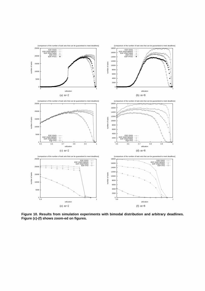
The results from the bimodal distribution are shown in Figure 8-Figure 11. It can be seen that the new algorithm EDF-SS(x) performs significantly better than EDF-FFD.

The results from the uniform distribution are shown in Figure 12-Figure 15. The results from the exponential distributionare shown in Figure 16-Figure 19. The conclusion is the same;the new algorithm EDF-SS(x) performs significantly betterthan EDF-FFD.

0

5000

10000

15000

20000

25000

0 1

num

ber

of ta

sks

utilization




EDF-FFDUEhd2-SIP

(a) m=2

0

2000

4000

6000

8000

10000

12000

14000

16000

18000

20000

0 1

num

ber

of ta

sks

utilization




EDF-FFDUEhd2-SIP

(b) m=8

0

5000

10000

15000

20000

25000

0.5 0.6 0.7 0.8 0.9 1

num

ber

of ta

sks

utilization



EDF-SS(DTMIN)EDF-FFDEhd2-SIP

(c) m=2

0

2000

4000

6000

8000

10000

12000

14000

16000

18000

20000

0.5 0.6 0.7 0.8 0.9 1

num

ber

of ta

sks

utilization




(d) m=8

0

5000

10000

15000

20000

25000

0.9 1

num

ber

of ta

sks

utilization




(e) m=2

0

2000

4000

6000

8000

10000

12000

14000

16000

18000

0.9 1

num

ber

of ta

sks

utilization




(f) m=8

Figure 8. Results from simulation experiments with bimodal distribution and implicit deadlines. Fig-ure (c)-(f) shows zoom-ed on figures.

0

2000

4000

6000

8000

10000

12000

14000

16000

0 1

num

ber

of ta

sks

utilization




EDF-FFDU

(a) m=2

0

2000

4000

6000

8000

10000

12000

14000

16000

18000

0 1

num

ber

of ta

sks

utilization




EDF-FFDU

(b) m=8

0

2000

4000

6000

8000

10000

12000

14000

16000

0.5 0.6 0.7 0.8 0.9 1

num

ber

of ta

sks

utilization




(c) m=2

0

2000

4000

6000

8000

10000

12000

14000

16000

18000

0.5 0.6 0.7 0.8 0.9 1

num

ber

of ta

sks

utilization




(d) m=8

0

1000

2000

3000

4000

5000

6000

0.9 1

num

ber

of ta

sks

utilization




(e) m=2

0

200

400

600

800

1000

1200

0.9 1

num

ber

of ta

sks

utilization




(f) m=8

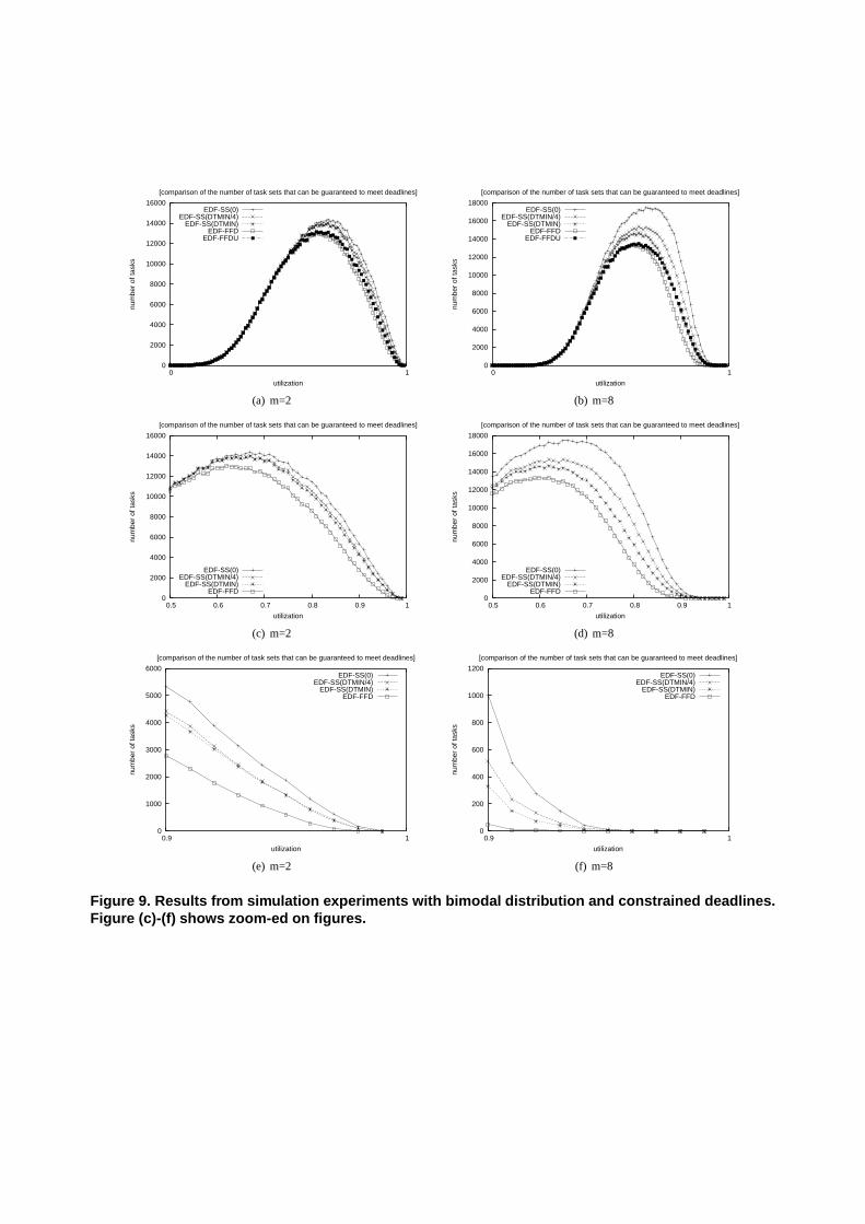
Figure 9. Results from simulation experiments with bimodal distribution and constrained deadlines.Figure (c)-(f) shows zoom-ed on figures.

0

5000

10000

15000

20000

25000

0 1

num

ber

of ta

sks

utilization




EDF-FFDU

(a) m=2

0

2000

4000

6000

8000

10000

12000

14000

16000

18000

0 1

num

ber

of ta

sks

utilization




EDF-FFDU

(b) m=8

0

5000

10000

15000

20000

25000

0.5 0.6 0.7 0.8 0.9 1

num

ber

of ta

sks

utilization




(c) m=2

0

2000

4000

6000

8000

10000

12000

14000

16000

18000

0.5 0.6 0.7 0.8 0.9 1

num

ber

of ta

sks

utilization




(d) m=8

0

5000

10000

15000

20000

25000

0.9 1

num

ber

of ta

sks

utilization




(e) m=2

0

2000

4000

6000

8000

10000

12000

14000

16000

18000

0.9 1

num

ber

of ta

sks

utilization




(f) m=8

Figure 10. Results from simulation experiments with bimoda l distribution and arbitrary deadlines.Figure (c)-(f) shows zoom-ed on figures.

0

5000

10000

15000

20000

25000

0 1

num

ber

of ta

sks

utilization




EDF-FFDU

(a) m=2

0

2000

4000

6000

8000

10000

12000

14000

16000

18000

0 1

num

ber

of ta

sks

utilization




EDF-FFDU

(b) m=8

0

5000

10000

15000

20000

25000

0.5 0.6 0.7 0.8 0.9 1

num

ber

of ta

sks

utilization




(c) m=2

0

2000

4000

6000

8000

10000

12000

14000

16000

18000

0.5 0.6 0.7 0.8 0.9 1

num

ber

of ta

sks

utilization




(d) m=8

0

5000

10000

15000

20000

25000

0.9 1

num

ber

of ta

sks

utilization




(e) m=2

0

2000

4000

6000

8000

10000

12000

14000

16000

18000

0.9 1

num

ber

of ta

sks

utilization




(f) m=8

Figure 11. Results from simulation experiments with bimoda l distribution and arbitrary deadlines(superperiod). Figure (c)-(f) shows zoom-ed on figures.

0

5000

10000

15000

20000

25000

30000

0 1

num

ber

of ta

sks

utilization




EDF-FFDUEhd2-SIP

(a) m=2

0

5000

10000

15000

20000

25000

0 1

num

ber

of ta

sks

utilization




EDF-FFDUEhd2-SIP

(b) m=8

0

5000

10000

15000

20000

25000

30000

0.5 0.6 0.7 0.8 0.9 1

num

ber

of ta

sks

utilization




(c) m=2

0

5000

10000

15000

20000

25000

0.5 0.6 0.7 0.8 0.9 1

num

ber

of ta

sks

utilization




(d) m=8

0

5000

10000

15000

20000

25000

30000

0.9 1

num

ber

of ta

sks

utilization




(e) m=2

0

5000

10000

15000

20000

25000

0.9 1

num

ber

of ta

sks

utilization




(f) m=8

Figure 12. Results from simulation experiments with unifor m distribution and implicit deadlines.Figure (c)-(f) shows zoom-ed on figures.

0

2000

4000

6000

8000

10000

12000

14000

16000

0 1

num

ber

of ta

sks

utilization




EDF-FFDU

(a) m=2

0

5000

10000

15000

20000

25000

0 1

num

ber

of ta

sks

utilization




EDF-FFDU

(b) m=8

0

2000

4000

6000

8000

10000

12000

14000

16000

0.5 0.6 0.7 0.8 0.9 1

num

ber

of ta

sks

utilization




(c) m=2

0

5000

10000

15000

20000

25000

0.5 0.6 0.7 0.8 0.9 1

num

ber

of ta

sks

utilization




(d) m=8

0

1000

2000

3000

4000

5000

6000

7000

8000

0.9 1

num

ber

of ta

sks

utilization




(e) m=2

0

500

1000

1500

2000

2500

0.9 1

num

ber

of ta

sks

utilization




(f) m=8

Figure 13. Results from simulation experiments with unifor m distribution and constrained deadlines.Figure (c)-(f) shows zoom-ed on figures.

0

5000

10000

15000

20000

25000

0 1

num

ber

of ta

sks

utilization




EDF-FFDU

(a) m=2

0

5000

10000

15000

20000

25000

0 1

num

ber

of ta

sks

utilization




EDF-FFDU

(b) m=8

0

5000

10000

15000

20000

25000

0.5 0.6 0.7 0.8 0.9 1

num

ber

of ta

sks

utilization




(c) m=2

0

5000

10000

15000

20000

25000

0.5 0.6 0.7 0.8 0.9 1

num

ber

of ta

sks

utilization




(d) m=8

0

5000

10000

15000

20000

25000

0.9 1

num

ber

of ta

sks

utilization




(e) m=2

0

5000

10000

15000

20000

25000

0.9 1

num

ber

of ta

sks

utilization




(f) m=8

Figure 14. Results from simulation experiments with unifor m distribution and arbitrary deadlines.Figure (c)-(f) shows zoom-ed on figures.

0

5000

10000

15000

20000

25000

30000

0 1

num

ber

of ta

sks

utilization




EDF-FFDU

(a) m=2

0

5000

10000

15000

20000

25000

0 1

num

ber

of ta

sks

utilization




EDF-FFDU

(b) m=8

0

5000

10000

15000

20000

25000

30000

0.5 0.6 0.7 0.8 0.9 1

num

ber

of ta

sks

utilization




(c) m=2

0

5000

10000

15000

20000

25000

0.5 0.6 0.7 0.8 0.9 1

num

ber

of ta

sks

utilization




(d) m=8

0

5000

10000

15000

20000

25000

30000

0.9 1

num

ber

of ta

sks

utilization




(e) m=2

0

5000

10000

15000

20000

25000

0.9 1

num

ber

of ta

sks

utilization




(f) m=8

Figure 15. Results from simulation experiments with unifor m distribution and arbitrary deadlines(superperiod). Figure (c)-(f) shows zoom-ed on figures.

0

5000

10000

15000

20000

25000

0 1

num

ber

of ta

sks

utilization




EDF-FFDUEhd2-SIP

(a) m=2

0

2000

4000

6000

8000

10000

12000

14000

16000

18000

20000

0 1

num

ber

of ta

sks

utilization




EDF-FFDUEhd2-SIP

(b) m=8

0

5000

10000

15000

20000

25000

0.5 0.6 0.7 0.8 0.9 1

num

ber

of ta

sks

utilization




(c) m=2

0

2000

4000

6000

8000

10000

12000

14000

16000

18000

20000

0.5 0.6 0.7 0.8 0.9 1

num

ber

of ta

sks

utilization




(d) m=8

0

5000

10000

15000

20000

25000

0.9 1

num

ber

of ta

sks

utilization




(e) m=2

0

2000

4000

6000

8000

10000

12000

14000

16000

18000

20000

0.9 1

num

ber

of ta

sks

utilization




(f) m=8

Figure 16. Results from simulation experiments with expone ntial distribution and implicit deadlines.Figure (c)-(f) shows zoom-ed on figures.

0

2000

4000

6000

8000

10000

12000

14000

16000

0 1

num

ber

of ta

sks

utilization




EDF-FFDU

(a) m=2

0

2000

4000

6000

8000

10000

12000

14000

16000

18000

0 1

num

ber

of ta

sks

utilization




EDF-FFDU

(b) m=8

0

2000

4000

6000

8000

10000

12000

14000

16000

0.5 0.6 0.7 0.8 0.9 1

num

ber

of ta

sks

utilization




(c) m=2

0

2000

4000

6000

8000

10000

12000

14000

16000

18000

0.5 0.6 0.7 0.8 0.9 1

num

ber

of ta

sks

utilization




(d) m=8

0

1000

2000

3000

4000

5000

6000

7000

8000

0.9 1

num

ber

of ta

sks

utilization




(e) m=2

0

500

1000

1500

2000

2500

3000

3500

4000

0.9 1

num

ber

of ta

sks

utilization




(f) m=8

Figure 17. Results from simulation experiments with expone ntial distribution and constrained dead-lines. Figure (c)-(f) shows zoom-ed on figures.

0

5000

10000

15000

20000

25000

0 1

num

ber

of ta

sks

utilization




EDF-FFDU

(a) m=2

0

2000

4000

6000

8000

10000

12000

14000

16000

18000

20000

0 1

num

ber

of ta

sks

utilization




EDF-FFDU

(b) m=8

0

5000

10000

15000

20000

25000

0.5 0.6 0.7 0.8 0.9 1

num

ber

of ta

sks

utilization




(c) m=2

0

2000

4000

6000

8000

10000

12000

14000

16000

18000

20000

0.5 0.6 0.7 0.8 0.9 1

num

ber

of ta

sks

utilization




(d) m=8

0

5000

10000

15000

20000

25000

0.9 1

num

ber

of ta

sks

utilization




(e) m=2

0

2000

4000

6000

8000

10000

12000

14000

16000

18000

20000

0.9 1

num

ber

of ta

sks

utilization




(f) m=8

Figure 18. Results from simulation experiments with expone ntial distribution and arbitrary deadlines.Figure (c)-(f) shows zoom-ed on figures.

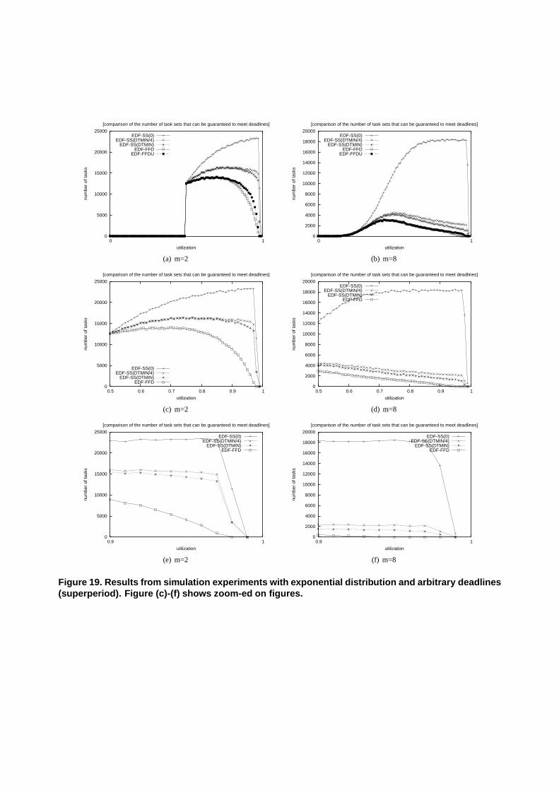
0

5000

10000

15000

20000

25000

0 1

num

ber

of ta

sks

utilization




EDF-FFDU

(a) m=2

0

2000

4000

6000

8000

10000

12000

14000

16000

18000

20000

0 1

num

ber

of ta

sks

utilization




EDF-FFDU

(b) m=8

0

5000

10000

15000

20000

25000

0.5 0.6 0.7 0.8 0.9 1

num

ber

of ta

sks

utilization




(c) m=2

0

2000

4000

6000

8000

10000

12000

14000

16000

18000

20000

0.5 0.6 0.7 0.8 0.9 1

num

ber

of ta

sks

utilization




(d) m=8

0

5000

10000

15000

20000

25000

0.9 1

num

ber

of ta

sks

utilization




(e) m=2

0

2000

4000

6000

8000

10000

12000

14000

16000

18000

20000

0.9 1

num

ber

of ta

sks

utilization




(f) m=8

Figure 19. Results from simulation experiments with expone ntial distribution and arbitrary deadlines(superperiod). Figure (c)-(f) shows zoom-ed on figures.

HURRAY TR 080501

Documents

Transcript of HURRAY TR 080501