Hunters Point Community Microgrid Project Power … Point Community Microgrid Project Power Flow...
36
Hunters Point Community Microgrid Project Power Flow Analysis Methodology A Distribution Grid, Dynamic Power Flow Modeling Case Study
-
Upload
nguyenliem -
Category
Documents
-
view
220 -
download
5
Transcript of Hunters Point Community Microgrid Project Power … Point Community Microgrid Project Power Flow...

Hunters Point Community Microgrid Project
Power Flow Analysis Methodology
A Distribution Grid, Dynamic Power Flow Modeling Case Study

____________________________________________________________________________________________ © 2016 Clean Coalition | www.clean-coalition.org 2
Acknowledgements
The following organizations have provided a great deal of support through training, applications,
data, and suggestions for this paper.
CYME International T&D, a division of Eaton
Pacific Gas and Electric Company
Integral Analytics, Inc.
The Clean Coalition is deeply grateful to the following for their support of the Hunters Point
Community Microgrid Project.
Common Sense Fund
Threshold Foundation, Sustainable Planet Funding Circle
The 11th Hour Project
The San Francisco Foundation
Wells Fargo Foundation
____________________________________________________________________________________________ © 2016 Clean Coalition | www.clean-coalition.org 3
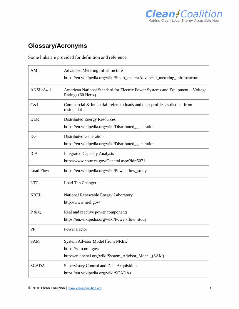
Glossary/Acronyms
Some links are provided for definition and reference.
AMI Advanced Metering Infrastructure
https://en.wikipedia.org/wiki/Smart_meter#Advanced_metering_infrastructure
ANSI c84-1 American National Standard for Electric Power Systems and Equipment – Voltage
Ratings (60 Hertz)
C&I Commercial & Industrial: refers to loads and their profiles as distinct from
residential
DER Distributed Energy Resources
https://en.wikipedia.org/wiki/Distributed_generation
DG Distributed Generation
https://en.wikipedia.org/wiki/Distributed_generation
ICA Integrated Capacity Analysis
http://www.cpuc.ca.gov/General.aspx?id=5071
Load Flow https://en.wikipedia.org/wiki/Power-flow_study
LTC Load Tap Changer
NREL National Renewable Energy Laboratory
http://www.nrel.gov/
P & Q Real and reactive power components
https://en.wikipedia.org/wiki/Power-flow_study
PF Power Factor
SAM System Advisor Model [from NREL]
https://sam.nrel.gov/
http://en.openei.org/wiki/System_Advisor_Model_(SAM)
SCADA Supervisory Control and Data Acquisition
https://en.wikipedia.org/wiki/SCADAs

____________________________________________________________________________________________ © 2016 Clean Coalition | www.clean-coalition.org 4
Table of Contents
Hunters Point Community Microgrid Project ........................................................................... 1
Power Flow Analysis Methodology ............................................................................................. 1
A Distribution Grid, Dynamic Power Flow Modeling Case Study .......................................... 1
Acknowledgements ....................................................................................................................... 2
Glossary/Acronyms ....................................................................................................................... 3
Background ................................................................................................................................... 6 Hunters Point Substation ....................................................................................................................... 6
Methodology ................................................................................................................................ 10 Metrics and Output .............................................................................................................................. 12 Establishing a Baseline ......................................................................................................................... 12 Effect of Adding DG ............................................................................................................................. 12 Siting the PV ......................................................................................................................................... 13 Assessing Capacity to add DG to Hunters Point Grid ...................................................................... 15 Voltage Regulation in Action ............................................................................................................... 19 Other DER Methods ............................................................................................................................. 21 Forcing Out-of-Range Voltages ........................................................................................................... 21
Conclusion ................................................................................................................................... 22 Significant Findings .............................................................................................................................. 22 Six Step Methodology ........................................................................................................................... 22 Capacity Planning Cost Effectiveness ................................................................................................. 23 Impact .................................................................................................................................................... 24
Appendix A: Data Processing to Support Dynamic Load Flows ............................................ 25 Modeling Platform ................................................................................................................................ 25 Problems to be Solved .......................................................................................................................... 25
Examples ............................................................................................................................................ 25 Solutions/limitations/work arounds/consequences ............................................................................ 26
Data limitations .................................................................................................................................. 26 Static vs Dynamic (Time Based) Load Flow Modeling ..................................................................... 26 Network Model ..................................................................................................................................... 27
Discrete Feeder Model ....................................................................................................................... 27 Substation Model................................................................................................................................ 27 Testing the Model............................................................................................................................... 27
Determining Load and Generation Profiles ....................................................................................... 28 Generation .......................................................................................................................................... 28 Loads .................................................................................................................................................. 28 Validation of Complete Circuit Model ............................................................................................... 30 Performing Dynamic Load Flow Runs .............................................................................................. 33
Other Assumptions, Issues ................................................................................................................... 35 Long Term Dynamics Modeling software ......................................................................................... 35 Network model conversion ................................................................................................................ 35
Appendix B: How Adding DG Affects Local Voltage.............................................................. 36
References .................................................................................................................................... 36
____________________________________________________________________________________________ © 2016 Clean Coalition | www.clean-coalition.org 5
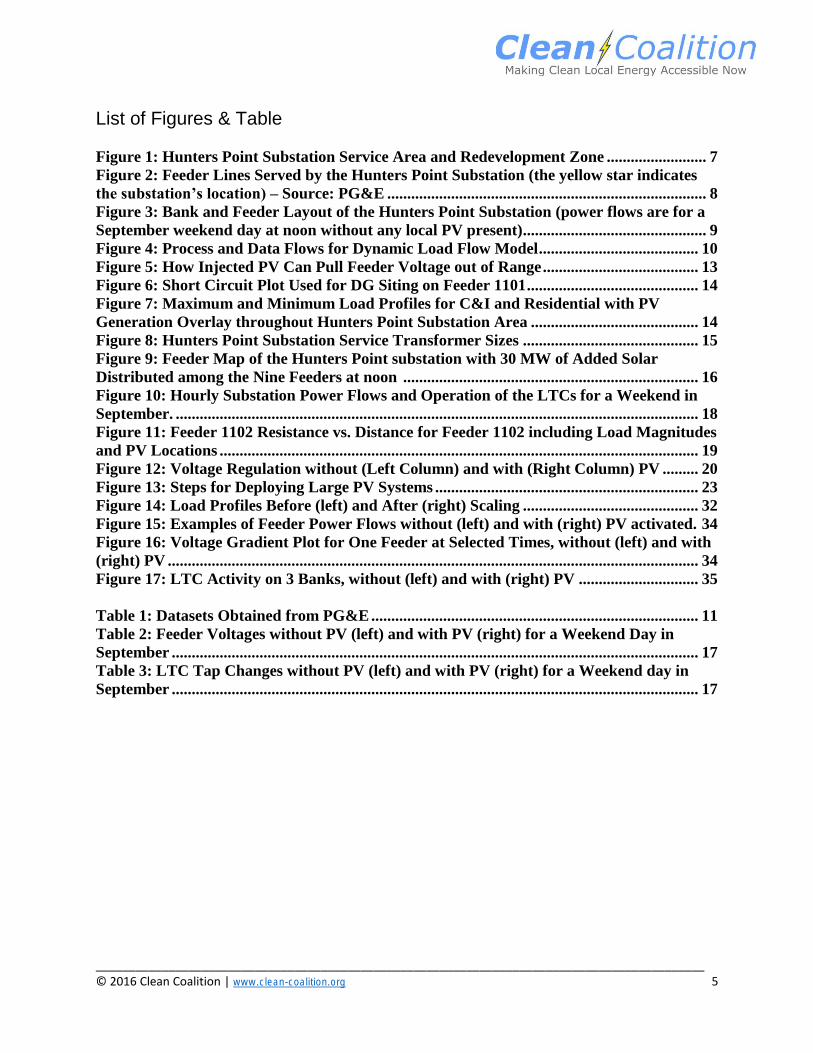
List of Figures & Table
Figure 1: Hunters Point Substation Service Area and Redevelopment Zone ......................... 7 Figure 2: Feeder Lines Served by the Hunters Point Substation (the yellow star indicates
the substation’s location) – Source: PG&E ................................................................................ 8
Figure 3: Bank and Feeder Layout of the Hunters Point Substation (power flows are for a
September weekend day at noon without any local PV present).............................................. 9 Figure 4: Process and Data Flows for Dynamic Load Flow Model ........................................ 10 Figure 5: How Injected PV Can Pull Feeder Voltage out of Range ....................................... 13 Figure 6: Short Circuit Plot Used for DG Siting on Feeder 1101 ........................................... 14
Figure 7: Maximum and Minimum Load Profiles for C&I and Residential with PV
Generation Overlay throughout Hunters Point Substation Area .......................................... 14 Figure 8: Hunters Point Substation Service Transformer Sizes ............................................ 15
Figure 9: Feeder Map of the Hunters Point substation with 30 MW of Added Solar
Distributed among the Nine Feeders at noon .......................................................................... 16 Figure 10: Hourly Substation Power Flows and Operation of the LTCs for a Weekend in
September. ................................................................................................................................... 18 Figure 11: Feeder 1102 Resistance vs. Distance for Feeder 1102 including Load Magnitudes
and PV Locations ........................................................................................................................ 19
Figure 12: Voltage Regulation without (Left Column) and with (Right Column) PV ......... 20 Figure 13: Steps for Deploying Large PV Systems .................................................................. 23
Figure 14: Load Profiles Before (left) and After (right) Scaling ............................................ 32 Figure 15: Examples of Feeder Power Flows without (left) and with (right) PV activated. 34 Figure 16: Voltage Gradient Plot for One Feeder at Selected Times, without (left) and with
(right) PV ..................................................................................................................................... 34
Figure 17: LTC Activity on 3 Banks, without (left) and with (right) PV .............................. 35
Table 1: Datasets Obtained from PG&E .................................................................................. 11
Table 2: Feeder Voltages without PV (left) and with PV (right) for a Weekend Day in
September .................................................................................................................................... 17
Table 3: LTC Tap Changes without PV (left) and with PV (right) for a Weekend day in
September .................................................................................................................................... 17

____________________________________________________________________________________________ © 2016 Clean Coalition | www.clean-coalition.org 6
Background
The United States’ power system, built on century-old technology and methods, was designed to deliver
electricity from large, remote power plants across significant distances to the cities and towns where
electricity is actually used. However, locally sited renewable energy generation has become economically
competitive with centralized generation and offers a superior approach for a vastly improved power
system.
To accelerate the deployment of high penetration distributed generation (DG), the Clean Coalition
established the Community Microgrid Initiative and undertaken the Hunters Point Community Microgrid
Project (HPCMP). The design criteria for the HPCMP is 1) achieving 25% of total energy consumed from
local renewables, while 2) at least maintaining grid reliability and power quality. This study covers the
power flow analysis modeling that was undertaken to simulate the design criteria.
The Clean Coalition collaborated with Pacific Gas & Electric (PG&E) and CYME International T&D to
demonstrate that existing grid modeling software can ensure a stable, effective distribution grid
containing high penetration PV. This power flow analysis case study was undertaken in coordination with
the City of San Francisco and PGE&E.
Hunters Point Substation
The Bayview Hunters Point (BVHP) area of San Francisco encompasses an extensive, existing urban
infrastructure, including a wastewater treatment plant, a large recycling facility, and significant
commercial, industrial, and residential buildings. The area also includes the former Hunters Point Naval
Shipyard that is being redeveloped with new urban, mixed use (residential and commercial) construction.
PG&E Hunters Point substation provides approximately 20,000 BVHP customers with electrical power.
Of those customers, 90% are residential and 10% are commercial/industrial (C&I) by customer type, but
loads are mostly C&I, as is shown later in Figure 7.
The HPCMP had a PV penetration goal of 25% of total electric energy for BVHP from local renewables.
This translates to about 30 MW for the substation boundary area, not including the part planned for
redevelopment (see Figure 1). If the redevelopment area is included, 50 MW (60,000 MWh) of
renewable generation is necessary to achieve the 25% goal. Existing and/or renewables planned for the
redevelopment area total around 20 MW, leaving 30 MW of new generation to meet the 25% goal in both
instances. Of critical importance is that this new power be sited such that the impact on grid reliability
and power quality is neutral or enhanced.
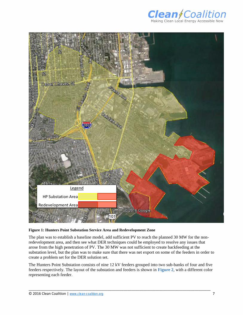
____________________________________________________________________________________________ © 2016 Clean Coalition | www.clean-coalition.org 7
Figure 1: Hunters Point Substation Service Area and Redevelopment Zone
The plan was to establish a baseline model, add sufficient PV to reach the planned 30 MW for the non-
redevelopment area, and then see what DER techniques could be employed to resolve any issues that
arose from the high penetration of PV. The 30 MW was not sufficient to create backfeeding at the
substation level, but the plan was to make sure that there was net export on some of the feeders in order to
create a problem set for the DER solution set.
The Hunters Point Substation consists of nine 12 kV feeders grouped into two sub-banks of four and five
feeders respectively. The layout of the substation and feeders is shown in Figure 2, with a different color
representing each feeder.
HP Substation Area
Redevelopment Area
Legend
____________________________________________________________________________________________ © 2016 Clean Coalition | www.clean-coalition.org 8
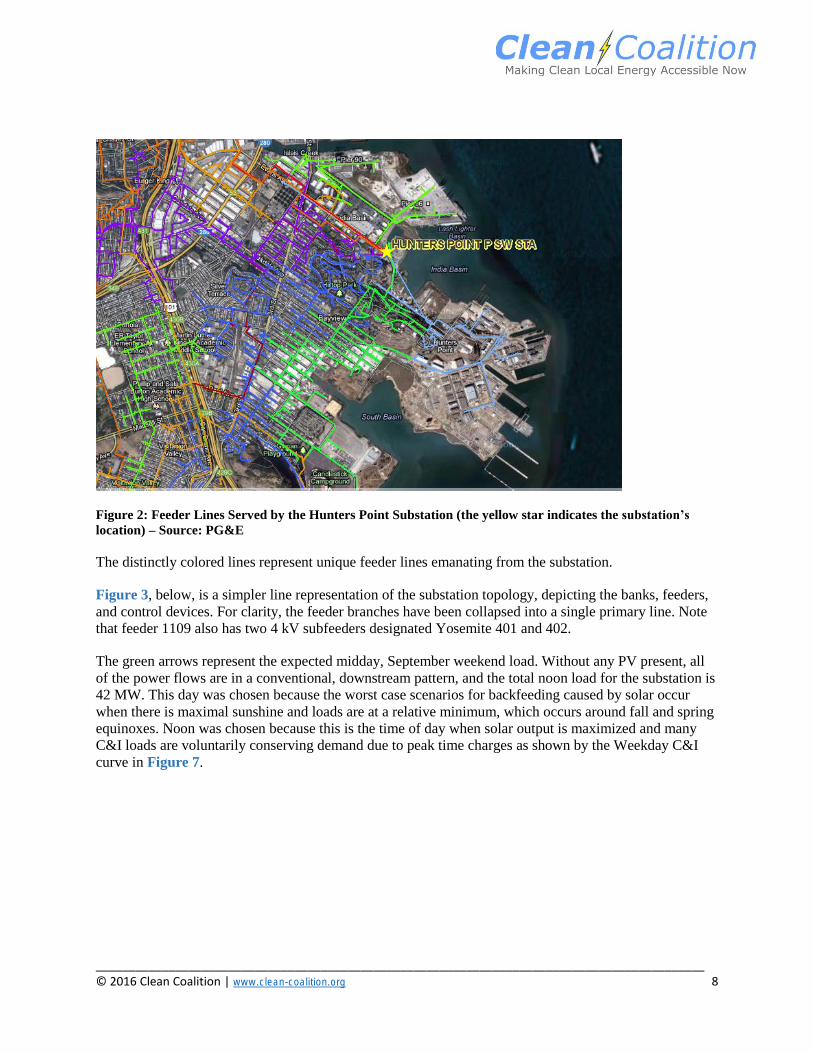
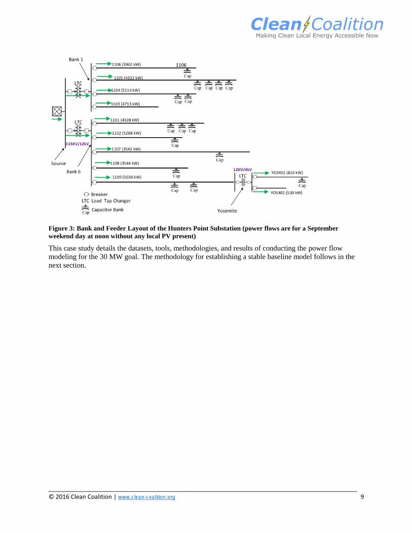
Figure 2: Feeder Lines Served by the Hunters Point Substation (the yellow star indicates the substation’s
location) – Source: PG&E
The distinctly colored lines represent unique feeder lines emanating from the substation.
Figure 3, below, is a simpler line representation of the substation topology, depicting the banks, feeders,
and control devices. For clarity, the feeder branches have been collapsed into a single primary line. Note
that feeder 1109 also has two 4 kV subfeeders designated Yosemite 401 and 402.
The green arrows represent the expected midday, September weekend load. Without any PV present, all
of the power flows are in a conventional, downstream pattern, and the total noon load for the substation is
42 MW. This day was chosen because the worst case scenarios for backfeeding caused by solar occur
when there is maximal sunshine and loads are at a relative minimum, which occurs around fall and spring
equinoxes. Noon was chosen because this is the time of day when solar output is maximized and many
C&I loads are voluntarily conserving demand due to peak time charges as shown by the Weekday C&I
curve in Figure 7.
____________________________________________________________________________________________ © 2016 Clean Coalition | www.clean-coalition.org 9
Figure 3: Bank and Feeder Layout of the Hunters Point Substation (power flows are for a September
weekend day at noon without any local PV present)
This case study details the datasets, tools, methodologies, and results of conducting the power flow
modeling for the 30 MW goal. The methodology for establishing a stable baseline model follows in the
next section.
____________________________________________________________________________________________ © 2016 Clean Coalition | www.clean-coalition.org 10
Methodology
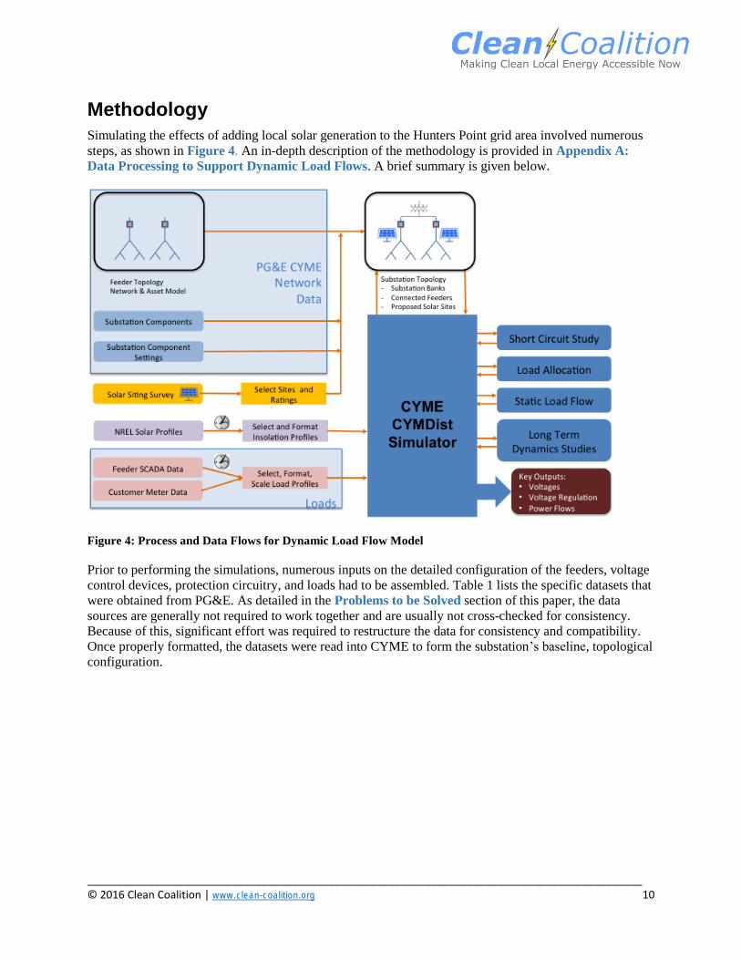
Simulating the effects of adding local solar generation to the Hunters Point grid area involved numerous
steps, as shown in Figure 4. An in-depth description of the methodology is provided in Appendix A:
Data Processing to Support Dynamic Load Flows. A brief summary is given below.
Figure 4: Process and Data Flows for Dynamic Load Flow Model
Prior to performing the simulations, numerous inputs on the detailed configuration of the feeders, voltage
control devices, protection circuitry, and loads had to be assembled. Table 1 lists the specific datasets that
were obtained from PG&E. As detailed in the Problems to be Solved section of this paper, the data
sources are generally not required to work together and are usually not cross-checked for consistency.
Because of this, significant effort was required to restructure the data for consistency and compatibility.
Once properly formatted, the datasets were read into CYME to form the substation’s baseline, topological
configuration.
____________________________________________________________________________________________ © 2016 Clean Coalition | www.clean-coalition.org 11
Dataset Format Description
Network Model CYME Data schema, lines, transformers (with ids), impedances, switches, fuses,
voltage regulators (e.g. LTCs, capacitors)
Asset Database CYME Transformer ids / switch ids / addresses / hardware parameters that may
be missing from Network Model
Network assets Excel Separate listings of such items as switch actions/settings, breaker trips,
regulator tap movements, capacitor switches, reclosers, voltage regulators,
existing distributed generation, seasonal loadings on transformers
Circuit map CYME Coordinate data is preferred for each element so that grid properties can
be displayed on Google Earth to see the effects of changes to the models.
Substation
SCADA Data
Excel Phase loads for each feeder as granular as possible with Power Factors
Customer
consumption /
load data
Excel Processed AMI data of load/consumption, monthly summary for four
different load types (Residential, Commercial, Industrial, Agricultural) by
weekday and weekend for 12 months
Table 1: Datasets Obtained from PG&E
The power flow simulation was performed using CYMDIST v5.04, a component of the CYME suite of
power modeling tools. The simulation is a four step process as described below. At each step, stability
must be achieved by correcting any issues uncovered before proceeding to the next step.
1) Short Circuit and Protection Test: The first step in the simulation is to perform a short circuit test.
This test quickly identifies weak areas of protection in the circuit configuration. Any protection
deficits have to be rectified before proceeding with load flow simulations. A typical finding
would be the absence of series reactors in the configuration of the substation.
2) Load Allocation: Load allocation is the process of partitioning power (kW) or current (Amps) per
phase load at a given point to the individual circuit elements down the line. It is a close
approximation to actual loading and is something of an art form. (Jennifer Taylor, 2009).
3) Static Load Flow: Static (single set of initial conditions) load flow runs must be performed to
validate the model before running dynamic load flows. The initial test is conducted with
distributed generation disabled. After a stable run is completed, DG can be enabled and then
gradually increased to full output to verify no new voltage or other capacity issues are caused by
the DG.
4) Dynamic Load Flow: CYMEDIST’s Dynamic Load Flow module runs a series of load flows with
time-based profiles for load and generation. The simulation provides detailed information on the
grid operating under real, dynamic conditions. Specific outputs include voltages, load flows, and
voltage regulating operation. All of the simulations reported below were performed with the
Dynamic Load Flow Module.
Once a stable configuration was established, we performed a baseline analysis of the grid without any DG
present and then began adding DG to the grid. As with the previous steps, the overall system must be
stable and any anomalous behavior must be resolved before moving forward. Comparisons were made
between weekday and weekend operation. A mid-September timeframe was chosen as the time most

____________________________________________________________________________________________ © 2016 Clean Coalition | www.clean-coalition.org 12
likely to create issues with good solar power and minimal loads to create the greatest seasonal variation
with high DG penetration.
Metrics and Output
The simulation reported several key outputs:
Voltages at key monitoring points along each feeder
Power flow magnitude, phase, and direction
Activity for all voltage regulating equipment (LTCs & capacitor banks)
These outputs also served as the primary metrics for comparing one configuration to another. The metrics
are summarized below:
Voltage: Voltage monitoring points were located at key components and some chosen nodes. Min, Max,
and Average voltages were summarized. Voltages were considered in-range if they were within the ANSI
c84-1 spec of ± 5% of the nominal voltage.
Power Flow: The magnitude of the power flow was monitored to ensure consistency with the load
profiles. Any change in power factor, direction, cross-feeding, or backfeeding was also noted.
Voltage regulation: Tap counts were recorded for load tap changers. The tap changers were also
monitored to ensure that they were not stuck at their min or max settings. Capacitor banks were also
monitored to ensure proper operation of those that could sense voltage to switch on/off.
Circuit Components: In addition to the above metrics, all circuit components were monitored for normal
operation and potential exceptions. Once stable runs were achieved, it was not likely that any component
ratings would be exceeded, but these were monitored, nonetheless.
Establishing a Baseline
The baseline power flow for a September weekend day is shown in Figure 3. This case was run without
any additional DG. Performing baseline runs is a critical step before assessing the impacts of local
renewables. The baseline case provides the point of comparison for all subsequent simulations and must
have a stable and repeatable outcome.
Effect of Adding DG
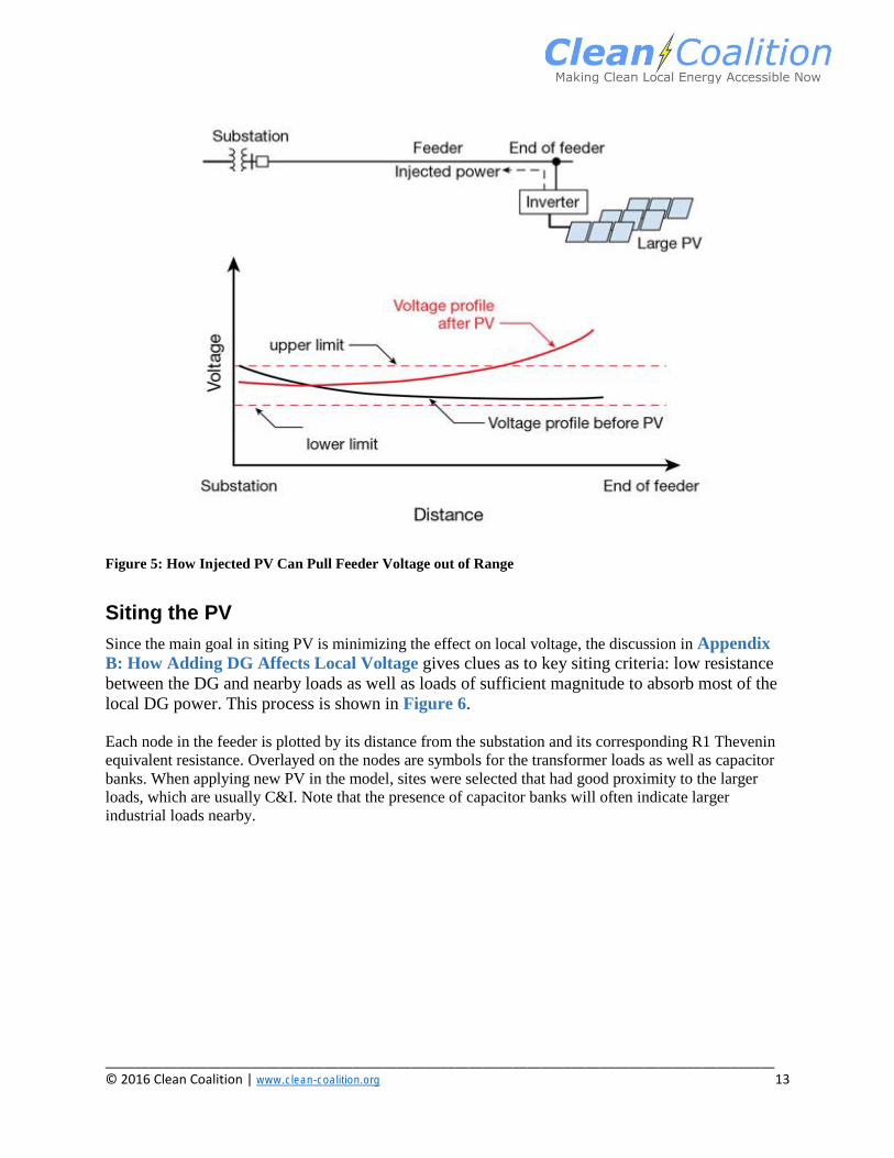
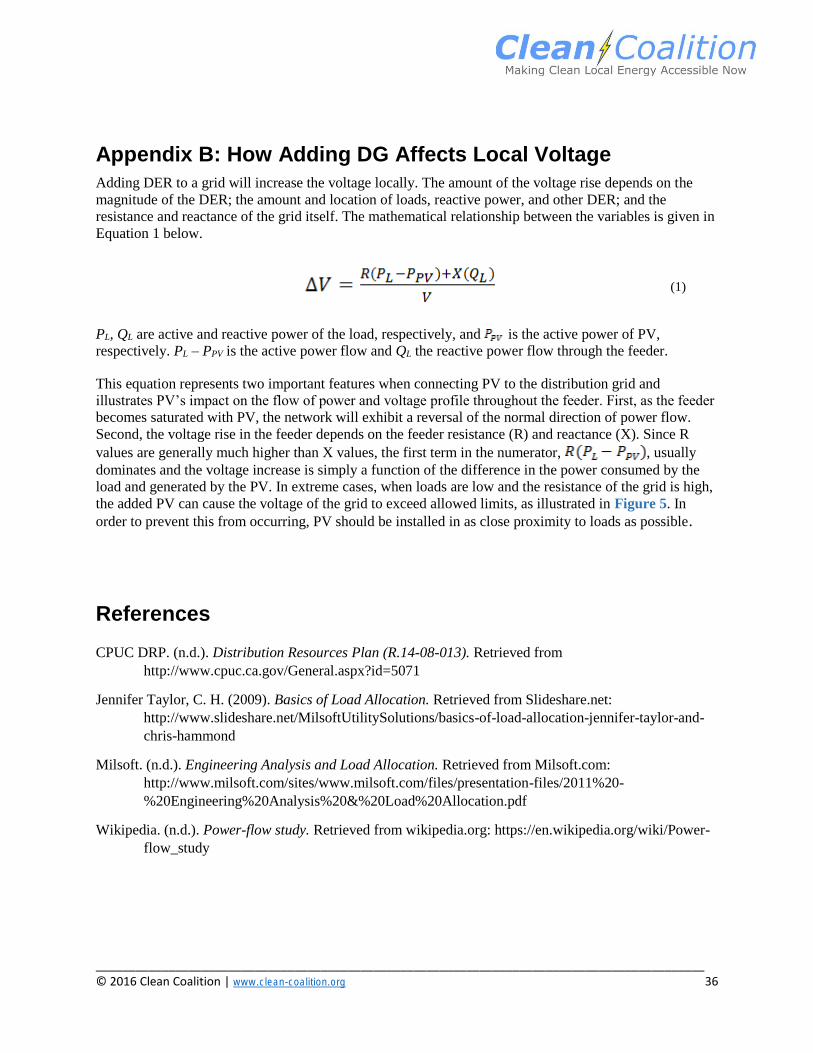
Adding DER to a grid will increase the voltage locally as shown in Figure 5. The amount of the voltage
rise depends on the magnitude of the DER, the amount and location of loads, reactive power, other DER,
and the resistance and reactance of the grid itself. A more detailed explanation is given in Appendix B:
How Adding DG Affects Local Voltage.
____________________________________________________________________________________________ © 2016 Clean Coalition | www.clean-coalition.org 13
Figure 5: How Injected PV Can Pull Feeder Voltage out of Range
Siting the PV
Since the main goal in siting PV is minimizing the effect on local voltage, the discussion in Appendix
B: How Adding DG Affects Local Voltage gives clues as to key siting criteria: low resistance
between the DG and nearby loads as well as loads of sufficient magnitude to absorb most of the
local DG power. This process is shown in Figure 6.
Each node in the feeder is plotted by its distance from the substation and its corresponding R1 Thevenin
equivalent resistance. Overlayed on the nodes are symbols for the transformer loads as well as capacitor
banks. When applying new PV in the model, sites were selected that had good proximity to the larger
loads, which are usually C&I. Note that the presence of capacitor banks will often indicate larger
industrial loads nearby.
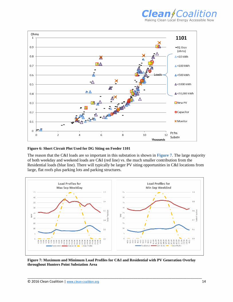
____________________________________________________________________________________________ © 2016 Clean Coalition | www.clean-coalition.org 14
Figure 6: Short Circuit Plot Used for DG Siting on Feeder 1101
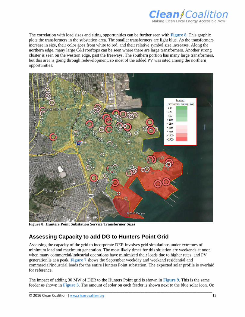
The reason that the C&I loads are so important in this substation is shown in Figure 7. The large majority
of both weekday and weekend loads are C&I (red line) vs. the much smaller contribution from the
Residential loads (blue line). There will typically be larger PV siting opportunities in C&I locations from
large, flat roofs plus parking lots and parking structures.
Figure 7: Maximum and Minimum Load Profiles for C&I and Residential with PV Generation Overlay
throughout Hunters Point Substation Area
____________________________________________________________________________________________ © 2016 Clean Coalition | www.clean-coalition.org 15
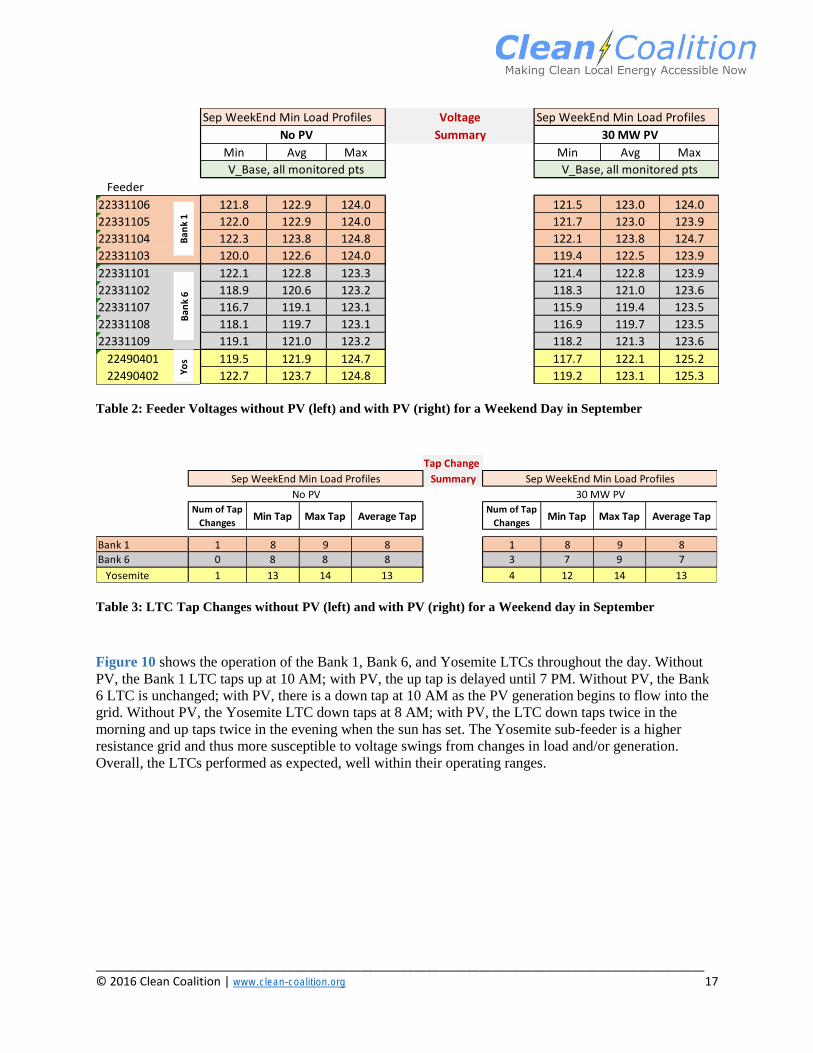
The correlation with load sizes and siting opportunities can be further seen with Figure 8. This graphic
plots the transformers in the substation area. The smaller transformers are light blue. As the transformers
increase in size, their color goes from white to red, and their relative symbol size increases. Along the
northern edge, many large C&I rooftops can be seen where there are large transformers. Another strong
cluster is seen on the western edge, past the freeways. The southern portion has many large transformers,
but this area is going through redevelopment, so most of the added PV was sited among the northern
opportunities.
Figure 8: Hunters Point Substation Service Transformer Sizes
Assessing Capacity to add DG to Hunters Point Grid
Assessing the capacity of the grid to incorporate DER involves grid simulations under extremes of
minimum load and maximum generation. The most likely times for this situation are weekends at noon
when many commercial/industrial operations have minimized their loads due to higher rates, and PV
generation is at a peak. Figure 7 shows the September weekday and weekend residential and
commercial/industrial loads for the entire Hunters Point substation. The expected solar profile is overlaid
for reference.
The impact of adding 30 MW of DER to the Hunters Point grid is shown in Figure 9. This is the same
feeder as shown in Figure 3. The amount of solar on each feeder is shown next to the blue solar icon. On

____________________________________________________________________________________________ © 2016 Clean Coalition | www.clean-coalition.org 16
four of the feeders, the added solar at noon is greater than the noon load and the normal power flow
direction is reversed as indicated by the red arrows. Power flows out of these feeders and crossfeeds to
serve loads on other feeders. Because the combined net load for the entire substation is greater than the
added 30 MW of PV, all of the PV is consumed within the Hunters Point substation and there is no power
backfeeding from the distribution to the transmission grid.
Figure 9: Feeder Map of the Hunters Point substation with 30 MW of Added Solar Distributed among the
Nine Feeders at noon
Note: green arrows indicate downstream power flow; red arrows indicate upstream power flow.
The grid remains within voltage limits even with the added PV. The existing voltage control devices
operate to smooth out any voltage variations, as seen in Table 2. With the added PV, the load tap
changers (LTC) experienced a slight increase in activity, as seen in Table 3. The Yosemite transformer
had one tap without added PV and four taps (two down, two up) with; Bank 1 had one without and one
with; Bank 6 had one without and three with.
____________________________________________________________________________________________ © 2016 Clean Coalition | www.clean-coalition.org 17
Sep WeekEnd Min Load Profiles Sep WeekEnd Min Load Profiles
No PV 30 MW PV
Min Avg Max Min Avg Max
V_Base, all monitored pts V_Base, all monitored pts
Feeder
22331106 121.8 122.9 124.0 121.5 123.0 124.0
22331105 122.0 122.9 124.0 121.7 123.0 123.9
22331104 122.3 123.8 124.8 122.1 123.8 124.7
22331103 120.0 122.6 124.0 119.4 122.5 123.9
22331101 122.1 122.8 123.3 121.4 122.8 123.9
22331102 118.9 120.6 123.2 118.3 121.0 123.6
22331107 116.7 119.1 123.1 115.9 119.4 123.5
22331108 118.1 119.7 123.1 116.9 119.7 123.5
22331109 119.1 121.0 123.2 118.2 121.3 123.6
22490401 119.5 121.9 124.7 117.7 122.1 125.2
22490402 122.7 123.7 124.8 119.2 123.1 125.3
Voltage
Summary
Ban
k 6
Yo
s B
ank
1
Table 2: Feeder Voltages without PV (left) and with PV (right) for a Weekend Day in September
Tap Change
Summary
Num of Tap
ChangesMin Tap Max Tap Average Tap
Num of Tap
ChangesMin Tap Max Tap Average Tap
Bank 1 1 8 9 8 1 8 9 8
Bank 6 0 8 8 8 3 7 9 7
Yosemite 1 13 14 13 4 12 14 13
Sep WeekEnd Min Load Profiles Sep WeekEnd Min Load Profiles
No PV 30 MW PV
Table 3: LTC Tap Changes without PV (left) and with PV (right) for a Weekend day in September
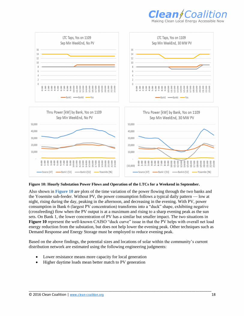
Figure 10 shows the operation of the Bank 1, Bank 6, and Yosemite LTCs throughout the day. Without
PV, the Bank 1 LTC taps up at 10 AM; with PV, the up tap is delayed until 7 PM. Without PV, the Bank
6 LTC is unchanged; with PV, there is a down tap at 10 AM as the PV generation begins to flow into the
grid. Without PV, the Yosemite LTC down taps at 8 AM; with PV, the LTC down taps twice in the
morning and up taps twice in the evening when the sun has set. The Yosemite sub-feeder is a higher
resistance grid and thus more susceptible to voltage swings from changes in load and/or generation.
Overall, the LTCs performed as expected, well within their operating ranges.
____________________________________________________________________________________________ © 2016 Clean Coalition | www.clean-coalition.org 18
Figure 10: Hourly Substation Power Flows and Operation of the LTCs for a Weekend in September.
Also shown in Figure 10 are plots of the time variation of the power flowing through the two banks and
the Yosemite sub-feeder. Without PV, the power consumption follows a typical daily pattern — low at
night, rising during the day, peaking in the afternoon, and decreasing in the evening. With PV, power
consumption in Bank 6 (largest PV concentration) transforms into a “duck” shape, exhibiting negative
(crossfeeding) flow when the PV output is at a maximum and rising to a sharp evening peak as the sun
sets. On Bank 1, the lower concentration of PV has a similar but smaller impact. The two situations in
Figure 10 represent the well-known CAISO “duck curve” issue in that the PV helps with overall net load
energy reduction from the substation, but does not help lower the evening peak. Other techniques such as
Demand Response and Energy Storage must be employed to reduce evening peak.
Based on the above findings, the potential sizes and locations of solar within the community’s current
distribution network are estimated using the following engineering judgments:
Lower resistance means more capacity for local generation
Higher daytime loads mean better match to PV generation
____________________________________________________________________________________________ © 2016 Clean Coalition | www.clean-coalition.org 19
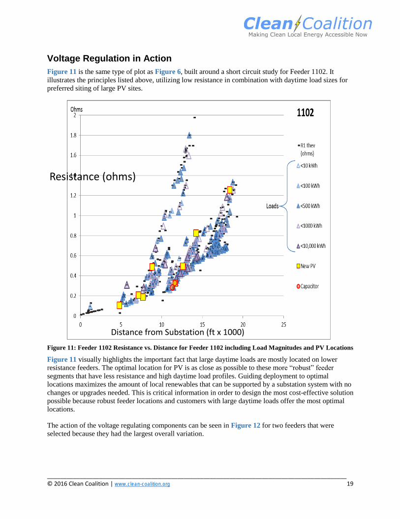
Voltage Regulation in Action
Figure 11 is the same type of plot as Figure 6, built around a short circuit study for Feeder 1102. It
illustrates the principles listed above, utilizing low resistance in combination with daytime load sizes for
preferred siting of large PV sites.
Figure 11: Feeder 1102 Resistance vs. Distance for Feeder 1102 including Load Magnitudes and PV Locations
Figure 11 visually highlights the important fact that large daytime loads are mostly located on lower
resistance feeders. The optimal location for PV is as close as possible to these more “robust” feeder
segments that have less resistance and high daytime load profiles. Guiding deployment to optimal
locations maximizes the amount of local renewables that can be supported by a substation system with no
changes or upgrades needed. This is critical information in order to design the most cost-effective solution
possible because robust feeder locations and customers with large daytime loads offer the most optimal
locations.
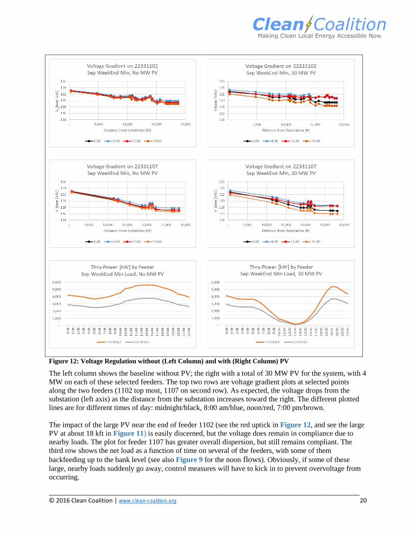
The action of the voltage regulating components can be seen in Figure 12 for two feeders that were
selected because they had the largest overall variation.
Distance from Substation (ft x 1000)
Resistance (ohms)
____________________________________________________________________________________________ © 2016 Clean Coalition | www.clean-coalition.org 20
Figure 12: Voltage Regulation without (Left Column) and with (Right Column) PV
The left column shows the baseline without PV; the right with a total of 30 MW PV for the system, with 4
MW on each of these selected feeders. The top two rows are voltage gradient plots at selected points
along the two feeders (1102 top most, 1107 on second row). As expected, the voltage drops from the
substation (left axis) as the distance from the substation increases toward the right. The different plotted
lines are for different times of day: midnight/black, 8:00 am/blue, noon/red, 7:00 pm/brown.
The impact of the large PV near the end of feeder 1102 (see the red uptick in Figure 12, and see the large
PV at about 18 kft in Figure 11) is easily discerned, but the voltage does remain in compliance due to
nearby loads. The plot for feeder 1107 has greater overall dispersion, but still remains compliant. The
third row shows the net load as a function of time on several of the feeders, with some of them
backfeeding up to the bank level (see also Figure 9 for the noon flows). Obviously, if some of these
large, nearby loads suddenly go away, control measures will have to kick in to prevent overvoltage from
occurring.

____________________________________________________________________________________________ © 2016 Clean Coalition | www.clean-coalition.org 21
Other DER Methods
It was assumed at the beginning of this project that advanced DER techniques ― such as smart inverters,
demand response, EV charging stations, and energy storage ― would be needed to enable the planned 30
MW of PV to function without causing voltage issues. It was a surprise to discover that the combination
of a network designed to service large C&I loads plus the profiles of the C&I loads were sufficient to
manage the voltage for this case.
The other DER techniques were simulated successfully using fixed sets of generation and load profiles to
verify they could be used to model these methods implicitly. Since this study was concluded, CYME has
added explicit DER features to support advanced inverters and energy storage directly in CYMDIST.
Forcing Out-of-Range Voltages
To verify that out-of-range voltages could be created in this configuration, changes were made to force
the error condition. Overvoltage was finally achieved by:
Increasing the additional PV from 30 W to 42 MW among the feeders.
Removing 12 MW of spot loads.
Freezing the LTCs near the high end of their range.
This amount of perturbation needed to force an error indicates a very robust and stable grid.

____________________________________________________________________________________________ © 2016 Clean Coalition | www.clean-coalition.org 22
Conclusion
Significant Findings
This case study emphasizes that this enormous asset ― the Hunters Point Substation Distribution Grid —
has significant underutilized capacity to accommodate local PV and other DER assets based on this
analysis. This capacity, and capability, should be realized in order to get the most out of our distribution
grid investment.
The biggest finding from the PV siting and the simulations is that existing load itself, along with low-
impedance access to that load, should be considered as resources when planning DER. This resource
already exists without any further effort and should be first on the list of considerations for planning.
For utility distribution planning, C&I customers can be an ideal match for DER programs, and especially
PV, in these important ways:
Maximum Generation Potential: C&I customers have larger rooftop and parking lot spaces that
can generate larger amounts of energy. Although some older buildings may have problems with
weight bearing of new PV systems, this issue can be addressed through newer light-weight
mounting systems or adding internal reinforcement to the roof structures.
Lower Costs: Larger PV systems at C&I locations are more cost-effective to deploy than smaller
residential rooftop systems, reducing overall system costs.
Best Locations: C&I customers typically use much larger loads and thus are connected to more
robust feeder segments. These more robust feeder segments are capable of handling more DER
without grid upgrades.
Matching Loads: C&I customers typically have larger daytime loads that match solar generation
profiles.
Financial Motivation: With proper feed-in tariffs, the owner of a C&I building can create a
guaranteed revenue stream that utilizes an asset, the roof, that normally does nothing more than
keep the rain out.
Given these five advantages, C&I customers offer the lowest hanging fruit to achieve scalable and cost-
effective DER deployments. Utilities seeking to achieve distributed generation goals quickly and cost-
effectively should design DER programs to leverage the C&I opportunity. Figure 7, above, helps
illustrate the value of a utility or community DER program focused on C&I customers. Note the load
shape for the C&I customer segment, which is the red line in the diagram. As a general rule, the load
requirements of the C&I customer segment reach an extended peak during the daytime, matching the
generation profile of PV much more closely than the residential customer segment.
Consuming all local DER within a substation’s distribution grid is a key aspect of the Hunters Point
Power Flow Analysis Methodology Case Study. These simulations demonstrate how excess power in one
part of the distribution grid can meet load demands in another part of the same distribution grid. The
added generation capacity can be accommodated by the existing loads and voltage control equipment. No
upgrades to the grid are required.
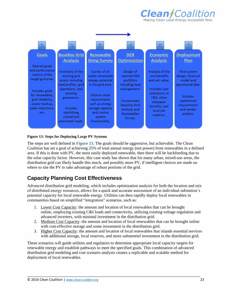
Six Step Methodology
As a result of this and other studies, the Clean Coalition recommends the following sequence for
deploying large amounts PV in small areas (substation level).
____________________________________________________________________________________________ © 2016 Clean Coalition | www.clean-coalition.org 23
Figure 13: Steps for Deploying Large PV Systems
The steps are well defined in Figure 13. The goals should be aggressive, but achievable. The Clean
Coalition has set a goal of achieving 25% of total annual energy (not power) from renewables in a defined
area. If this is done with PV, the most easily deployed renewable, then there will be backfeeding due to
the solar capacity factor. However, this case study has shown that for many urban, mixed-use areas, the
distribution grid can likely handle this much, and possibly more PV, if intelligent choices are made on
where to site the PV to take advantage of robust portions of the grid.
Capacity Planning Cost Effectiveness
Advanced distribution grid modeling, which includes optimization analysis for both the location and mix
of distributed energy resources, allows for a quick and accurate assessment of an individual substation’s
potential capacity for local renewable energy. Utilities can then rapidly deploy local renewables in
communities based on simplified “integration” scenarios, such as:
1. Lower Cost Capacity: the amount and location of local renewables that can be brought
online, employing existing C&I loads and connectivity, utilizing existing voltage regulation and
advanced inverters, with minimal investment in the distribution grid.
2. Medium Cost Capacity: the amount and location of local renewables that can be brought online
with cost-effective storage and some investment in the distribution grid.
3. Higher Cost Capacity: the amount and location of local renewables that islands essential services
with additional storage, local reserves, and more substantial investment in the distribution grid.
These scenarios will guide utilities and regulators to determine appropriate local capacity targets for
renewable energy and establish pathways to meet the specified goals. This combination of advanced
distribution grid modeling and cost scenario analysis creates a replicable and scalable method for
deployment of local renewables.

____________________________________________________________________________________________ © 2016 Clean Coalition | www.clean-coalition.org 24
The Hunters Point case study demonstrates that the distribution grid has the capacity to add significant
amounts of local renewables when they are properly sited utilizing existing grid assets.
Impact
We delivered the results and recommendations from this case study to PG&E, the City of San Francisco,
and the California Public Utilities Commission (CPUC). We used data from this case study to strengthen
implementation of Assembly Bill (AB) 327 ― first in the nation legislation requiring investor owned
utilities (IOUs) in California to identify optimal locations for the deployment of DER through distribution
resources plans. In November 2015, CPUC Commissioner Michael Picker issued draft guidance on AB
327 implementation through the CPUC’s Distribution Resources Plan proceeding, which incorporates
seven recommendations that come directly from this case study, including developing demonstration
projects. This in turn has led to the Integrated Capacity Analysis (ICA) requirement for California’s IOUs
to develop new methods to more accurately estimate the capacity of feeders to support various types of
DER and to make this information available to the public.
We also shared our case study results with officials in New York, as the State embarked on its ambitious
Reforming the Energy Vision proceeding. This case study was key to the development of new
requirements for New York utilities, which must now produce Distributed System Implementation Plans
that are very similar to distribution resources plans.
The existing process of evaluating local renewable energy projects one at a time is painstakingly slow and
introduces costly delays for these projects. By modeling large areas of the distribution grid, utilities and
regulators can efficiently identify greater DG opportunities and establish streamlined deployment plans.
This system-wide approach enables large amounts of local renewables to come online in months rather
than years.
____________________________________________________________________________________________ © 2016 Clean Coalition | www.clean-coalition.org 25
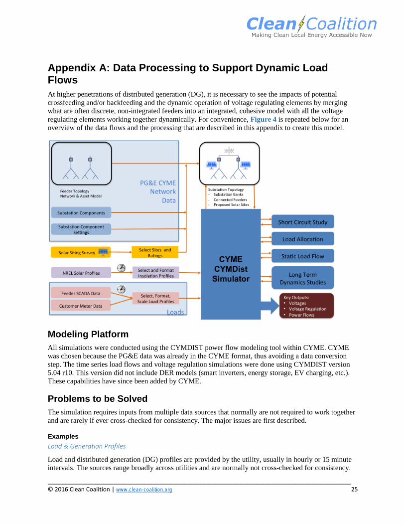
Appendix A: Data Processing to Support Dynamic Load Flows
At higher penetrations of distributed generation (DG), it is necessary to see the impacts of potential
crossfeeding and/or backfeeding and the dynamic operation of voltage regulating elements by merging
what are often discrete, non-integrated feeders into an integrated, cohesive model with all the voltage
regulating elements working together dynamically. For convenience, Figure 4 is repeated below for an
overview of the data flows and the processing that are described in this appendix to create this model.
Modeling Platform
All simulations were conducted using the CYMDIST power flow modeling tool within CYME. CYME
was chosen because the PG&E data was already in the CYME format, thus avoiding a data conversion
step. The time series load flows and voltage regulation simulations were done using CYMDIST version
5.04 r10. This version did not include DER models (smart inverters, energy storage, EV charging, etc.).
These capabilities have since been added by CYME.
Problems to be Solved
The simulation requires inputs from multiple data sources that normally are not required to work together
and are rarely if ever cross-checked for consistency. The major issues are first described.
Examples
Load & Generation Profiles
Load and distributed generation (DG) profiles are provided by the utility, usually in hourly or 15 minute
intervals. The sources range broadly across utilities and are normally not cross-checked for consistency.
____________________________________________________________________________________________ © 2016 Clean Coalition | www.clean-coalition.org 26
Various types of data are used for different purposes, and their normal applications do not normally
require correlation with other datasets.
Profiles by customer type
The best and most accurate load data is from Advanced Metering Infrastructure (AMI) data. Utilities
collect these data from all customers of all types. With AMI data it is possible to get a detailed breakdown
by customer type as long as the model is correctly configured. Integral Analytics provided anonymized
AMI data of the Hunters Point substation loads. The AMI data was scaled to match known peak loads
from the total substation SCADA data. Details on this methodology are discussed below in the Load
Profile Scaling section.
Absent AMI data, load information is obtained from SCADA feeder level profiles which do not break
loads down by customer type. The dynamic load flow can still be run successfully, but the insight from
customer type on different feeders and sections will not be available. See Load Profiles for more details.
Solutions/limitations/work arounds/consequences
The basic goal is to find the issues with the data and decide how to correct them, correlate them, or fill in
the missing components.
Data limitations
Many companies have adapted tools designed for transmission load flow studies to those targeted at the
distribution grid. When used for distribution grid studies, distribution components or details may have
been omitted from the models and now need to be added with newer tools that can take a more detailed
look at the distribution grid. Examples include substation components like load tap changers (LTC), bank
transformers, and series reactors. Without these components, the accuracy of modeling unbalanced loads
and similar issues is limited.
All companies have periodic upgrades of the tools they use to conduct operations. With each major
change, decisions must be made as to how much historical data will be transferred into the new formats
and verified. Assumptions have to be made as to content of new fields that were not present in the old
data set. As the data translations occur, data is often lost if it was not needed in the new platform or has
not been added if it did not prevent studies from being run. Over time, the troublesome networks are kept
up to date, but those that have not had many problems and have not much attention may be lacking in
detail in the network databases. The type of data that is missing determines the approach to replacement
or substitution.
Secondary Side Data
For the modeling, no secondary side data, other than load summaries by customer type at the transformer,
was available. When detailed customer load information is available, it may be necessary to create a
reduced dataset with the secondary information trimmed off and the net loads summed at the transformer
level. Doing so will minimize the number of issues that have to be resolved in initial debug of the dataset.
The section on Static Load Flow modeling discusses this in greater detail.
Static vs Dynamic (Time Based) Load Flow Modeling
Most utilities have focused their effort historically on static, worst-case load flows and have not yet
developed the expertise in-house for dealing with high levels of DG with time-of-day dependencies. In
some cases, work-arounds have been developed when varying values are needed, e.g. modeling each tap

____________________________________________________________________________________________ © 2016 Clean Coalition | www.clean-coalition.org 27
on a LTC and running separate load flows with different starting voltage conditions. Where customer
types are known but time data is not available, it is sometimes possible to use curves from other studies to
make reasonable estimates of the profile shapes and then make several runs to discover which ones are
the best match for the overall substation SCADA profiles.
Dynamic models like CYMDIST allow load flows and voltage changes to be simulated based on the time
of day, date, and time varying inputs (loads, insolation, etc.).
Network Model
Discrete Feeder Model
Utilities typically model distribution grids as distinct, disconnected feeders with no view of the banks or
other substation components. These models have been adequate in the past when DG penetration was
low. At higher penetrations of DG, it is necessary to see the impacts of potential crossfeeding and/or
backfeeding and the dynamic operation of voltage regulating elements.
Substation Model
Simulating crossfeeding and/or backfeeding requires a model of the substation topology, potentially up to
the interconnection with the transmission grid. The complexity of the model will vary depending upon
how far upstream, toward the transmission grid, the simulation is required to cover. The basic level will
be determined by how far backfeeding needs to be simulated. A bank level model is sufficient for
simulating crossfeeding between feeders. Joining the banks into a complete substation model is usually
straightforward and will cover most scenarios.
Substation Components
A reasonable representation of the substation is needed in order to see the effects of crossfeeding between
feeders in the same bank. Including bank transformers will improve the accuracy of the simulations.
Moving the driving point of the model upstream from the feeder headend through the transformer
impedances provides more “room” for the voltages to vary in a more realistic manner. Series Reactors are
needed in order to get reasonable values from short circuit studies. These can be added discretely, but
some programs allow adding them as integral properties of devices such as circuit breakers.
Voltage Regulator Settings
In addition to the transformer attributes, LTC attributes and settings are crucial to getting a stable model
that gives proper outputs under a wide variety of load conditions. It is important to match the control
connectivity choice that is being employed in the field. The model will not be stable until the voltage
regulator settings are accurate.
Capacitor Bank values and settings will also be critical. Most modeling programs allow options for fixed
on/off or voltage sensing on/off. Some allow scheduled settings.
Testing the Model
Testing the complete model with all the components and their settings is found in the section on
Validation of Complete Circuit Model.

____________________________________________________________________________________________ © 2016 Clean Coalition | www.clean-coalition.org 28
Determining Load and Generation Profiles
Seasonal worst case loads are normally used in load flow calculations. Cases to consider are:
Typical situations for calibration of loads, baseline (with DG off)
Max/Min loads
Min/Max generation
Generation
Generation profiles will come from sources associated with the type of generation. For renewables, there
are sources that can provide good statistical variety.
PV Profiles
The best source of information on expected PV profiles is NREL’s System Advisory Model (SAM). It
includes the effects of weather (clouds). One trick that can simplify other calculations is to run SAM for a
hypothetical 1 MW PV array at the location under consideration, then use the output as a scale factor for
other proposed site sizes.
The weather variability inherent in the model allows simulating multiple scenarios. The choice of day(s)
could include
Clear days for max solar
Cloudy days (minimal output)
Consecutive minimum days (worst case total energy sum)
Ps & Qs
Modeling programs generally allow generation and load profiles to be stated as either a magnitude and
phase angle or as real and reactive components. Updates to some programs are beginning to allow smart
inverter functionality with variable/controllable reactive power based upon various control profiles and
settings.
Siting DG
For a proposed site, the location is already determined. See Siting DG and DER for discussion on siting
for broader capacity studies.
Loads
Spot Loads
Commercial software vendors have very detailed methods for entering load data into their models.
Fixed value given in kW or kWh (or both)
Verify what statistic the spot load in the model represents: average over a period, max in a period, etc.
Given in model
Utilities employ processes that periodically populate the spot load data based upon billing information. It
is preferable to get both current and historical data to match the needs of the use cases that will be run.

____________________________________________________________________________________________ © 2016 Clean Coalition | www.clean-coalition.org 29
Load Profiles
The approach depends upon whether metered load data is available. The load data will be used to set up
corner cases with generation data, so choices should be made with this in mind.
For instance, load flows are often run with a focus on overall peak loading conditions. However, a worst
case condition for dynamic modeling is minimum loads with maximum PV near the noon hour, where
overvoltage is more likely. Also, the weekend and weekday profiles can be distinctly different depending
upon the mix of customer types found on different feeders (see Figure 7).
Metered Data available
Metered data is much more useful if it can be binned by customer type. It usually consists of:
Customer Type
Month or season
Weekday and Weekend
By hour or quarter hour
Choices of Summary Statistics
Load data can be summarized in many ways with differing statistics. Utilities already are expert at
extracting monthly or seasonal statistics for their own planning purposes. One very useful approach is to
create separate curves which represent profile probabilities, i.e. probabilities that at a given time
increment, the load value will be less than the stated value. Typical examples would be to use data for
peak loads and data for minimum loads.
No metered data available
Without AMI data, SCADA data from the substation must be used to create load profiles, but there will
be no independent representation by customer type.
SCADA Data
Like all other data sources, SCADA data needs to be screened and qualified. Companies may not be using
SCADA data for daily operational decisions, so there may be some holes and unique situations
represented in raw data.
Ps & Qs
Users of load flow modeling are already familiar with how each tool can accept complex power
representation. Choices will normally be either VA magnitude plus phase angle or separate P and Q
components.
Scaling
The statistical nature of the load profiles guarantees they will not sum up to any given daily load profile.
Therefore, they must be scaled to match the particular case/problem being analyzed.
Scaling of the load profiles cannot be done until dynamic power flow modeling is working, as described
in Static Load Flow.
Briefly, one must pick a reference point to scale to. Examples are peak load or total energy over some
interval. Peak load is normally chosen because it represents the most likely condition in which anomalies

____________________________________________________________________________________________ © 2016 Clean Coalition | www.clean-coalition.org 30
might occur that could be triggered in the simulations. Figure 14 shows how scaling is applied to load
profiles by customer type, in this case against peak load for the substation for the given conditions.
Validation of Complete Circuit Model
The model to be used should be validated using good engineering practice. A series of steps is normally
used to do this. For legacy models that have been transferred among various modeling tools over the
years, this process may uncover discrepancies and missing data that may need to rectified.
Short Circuit and Protection Tests
For feeders in stable areas, these tests may not have been done for a long time, and they provide a great
way to test how other components may have been dropped from the network model over the years.
Where discrete feeder models have been in use for some years, a common missing component are the
series reactors at the head end. This omission will be obvious by excessive currents in the short circuit
test. It may require digging through old records to find the values that need to be inserted. Any issues
should be rectified before proceeding with load flow models.
The studies should first be performed with DG off. After correcting any problems, they should then be
done with DG enabled to see if the new generators cause any problems.
One output of the short circuit studies that can be useful is the R1 Thevenin equivalent resistance from the
substation as will be discussed in Siting DG. It can be used for making visualization plots for PV siting
(Figure 6).
Running Balanced or Unbalanced
It is desirable to run the network model unbalanced to get greater detail, but very good insight can still be
obtained for typical networks running only balanced. If the phase details are not available, most
commercial programs will make reasonable assumptions for distributing the load on 2 and 1 phase
circuits.
Load Allocation
Load allocation is the process of partitioning power (kW) or current (Amps) per phase load at a given
point to the individual circuit elements down the line. It is a close approximation to actual loading and is
something of an art form. (Jennifer Taylor, 2009)
There are different ways of distributing the load, and modeling programs will assist with deciding upon
an allocation method based upon the type of analysis that will be done. (Milsoft)
The allocation must be done before load flow can be run.
Correct Allocation Problems
Typical problems found during allocation runs might include missing load values or locked loads that
must be unlocked in order to be adjusted. Plan on several runs if the feeders have not been examined in a
long time.

____________________________________________________________________________________________ © 2016 Clean Coalition | www.clean-coalition.org 31
Inputs and Outputs.
All of the network elements for a load flow are required. In addition to the network and its components,
some method of estimating the spot load on each transformer is needed. Typically billing data for power
(kW) or energy (kWh) is used, but transformer ratings can be used in the absence of billing data. The
modeling software will provide approaches to choose from based upon what data sources are available
(Jennifer Taylor, 2009). Most utilities have standardized processes for updating the seasonal loads in their
models.
The outputs will be updates to the model with properly allocated loads that are ready to run load flow
simulations.
Static Load Flow
Load flow is a numerical analysis of the flow of electric power in an interconnected system. (Wikipedia)
Static (single set of initial conditions) load flow runs must be performed to validate the model before
running dynamic load flows with time profiles that vary the conditions throughout a time period of
interest.
Additional inputs
Voltage Regulators
Voltage regulators can destabilize the model until their settings are correct. It is simpler to start the load
flow runs with the regulators disabled (set to a fixed point such as midpoint) until other issues have been
resolved. Once the runs are stable, the regulators can be enabled. Most programs allow the user to adjust
the initial settings of the regulators.
PV and Inverters
Solar PV usually has two main components in the model: DC power and inverter power. DG should be
Off or disconnected for initial runs until the circuit model is stable. When PV is enabled, some checks
must be done as to the relationship between PV DC ratings and inverter ratings.
When the DG is enabled, be sure to check how the system deals with oversized PV generation. Some
modeling programs will follow the insolation curve for the PV without regard to the constraints of the
inverter ratings. This can also happen when database conversion programs put in a default large value for
the PV panels with the intent of adjusting later when more detailed information is available. One work-
around to this problem is to drive the inverter from a generator curve rather than a PV insolation curve. It
may require several test runs to determine how the modeling program handles these situations and the
best way to handle it.
Voltage Check
Most commercial programs provide simple straightforward plots of voltage gradient as a function of
distance on a feeder for static load flow runs. These provide an excellent quick check on stability.
Selecting Nodes to Monitor
Some programs provide outputs for every node in the model for each run. In this case, the output will be
extremely large files that must be filtered for analysis.

____________________________________________________________________________________________ © 2016 Clean Coalition | www.clean-coalition.org 32
Other programs allow the user to select the points to monitor. Where points are being selected, a chart
such as Figure 6 becomes a useful tool. More detail is provided in Siting DG.
Dynamic Load Flow
Dynamic load flow runs a series of load flows with time-based profiles for load and generation that allow
a more detailed simulation of grid operation. It provides more detailed information about how the system,
especially the voltage regulating components, will behave under varying load and generation
combinations that are typical of daily operation.
Stability
It is important that the settings for regulating devices be accurate for the dynamic models to be stable
under all conditions. The system must first be made stable (all voltages in range and components
operating within limits) running a baseline load without DG activated. If the system is working in real
life, then the settings for the regulating equipment should work in the model.
If the model is not stable (voltages out of range, LTCs pegged at limits, oscillating, etc.), it must be
debugged. Settings on the voltage regulators are a typical culprit. Make sure that the monitoring points are
correct and that the type of connection/operating mode are correct. On LTCs, check to see if the taps have
reached their min/max limits; this could indicate errors in line drop compensation, such as R&X settings
or the point being monitored.
Load Profile Scaling
The advantage of dynamic load flow modeling is that the effects on non-coincident peaks among various
loads and sources can be examined. However, it does require that the profiles in use have a basis in the
known reality for those circuits. When different customer types with unique profiles are employed, it is
important to scale their profiles to match desired modeling conditions. As mentioned earlier, the max load
of the substation with DG Off is typically the easiest statistic to target. The same scale factor can be
applied to all customer type load profiles. It is an iterative process and will converge faster using a binary
search algorithm where the error around the target has both positive and negative values. Figure 14
shows an example of scaling a set of load profiles for different customer types for a given scenario.
Figure 14: Load Profiles Before (left) and After (right) Scaling

____________________________________________________________________________________________ © 2016 Clean Coalition | www.clean-coalition.org 33
Time Range
Different programs have different methods of managing time sequencing. The interval of coverage can
vary from hours to unlimited. The increments may be fixed throughout the simulation run or may allow
finer resolution around anticipated events. The load and generation profiles must be set up to match the
intended time intervals that each simulation run will cover. CYMDIST is set up to cover 24 hours with
resolution as fine as one second for observing the timings involved in voltage regulation elements.
Performing Dynamic Load Flow Runs
Siting DG and DER
For studies involving applications for specific sites, it is straightforward to add the DG to a specific
transformer in the model. For more general studies of potential of a section or feeder, siting has more
possibilities. Traditional fixed percentage rules of thumb for DG capacity limitations are based upon
assumptions around load profile shapes and need to be replaced by analytical approaches grounded in the
realities of each circuit’s characteristics. New tools are evolving, e.g. California’s Integrated Capacity
Analysis (ICA) that is built around circuit parameters and the profiles of loads and DG (CPUC DRP).
A visual method for selecting potential locations is shown in Figure 6. The black dots are the R1 values
from the Short Circuit Study plotted according to distance from the substation. The changes in slope
represent the changes in wire gauge along the feeder. Transformer loads of various groupings have been
plotted on the appropriate nodes as a reference. Existing capacitor banks are also shown and are usually
good indicators of industrial loads that can absorb a lot of daytime PV.
Also shown in Figure 6 are monitoring points that have been selected for output reports from the
modeling runs. A few well-placed points can yield significant insight with smaller datasets.
Inputs
The set of inputs for each run must be logged in order to allow reproducibility of results. Most
commercial programs have ways to save the entire set of inputs needed for particular studies. Notes
follow on a few items.
Voltage Regulator Settings
If the initial condition for voltage regulators is critical, then these should be recorded for the different
runs. Besides LTCs, settings for capacitor banks can be important.
Load & Generation Profiles
As the number of use case combinations rises it is tempting to make up many unique sets of profiles.
Where programs use drop down lists for selecting profiles, it can lead to very cluttered, slow, error prone
decisions each time a run is made. Some programs, e.g. CYME, only store the path name to the
designated profiles in the study file. This allows setting up some standardized corner case filenames for
the different cases and then changing the actual profile data to that needed for the month, season, or other
appropriate condition for a set of runs. However, good record keeping and consistent methodology is
required.
Time range to run
Most programs allow at least a 24-hour run duration. For those that allow longer runs, a 48-hour window
allows running with the typical maximum weekday load and minimum weekend load cases in the same
run, which can save time in running cases.

____________________________________________________________________________________________ © 2016 Clean Coalition | www.clean-coalition.org 34
Outputs
All programs can output real and reactive voltages and power for the nodes being monitored. It is
especially important to monitor the real power for signs of export. The negative power excursion in
Figure 15 with PV active is an example of export at the feeder level.
Figure 15: Examples of Feeder Power Flows without (left) and with (right) PV activated.
A set of voltage profiles for selected times can show the increased range of voltages that are caused by
large amounts of PV. Figure 16 shows the impact of PV on a feeder to increase the voltage dispersion,
especially from PV near the end of the feeder.
Figure 16: Voltage Gradient Plot for One Feeder at Selected Times, without (left) and with (right) PV
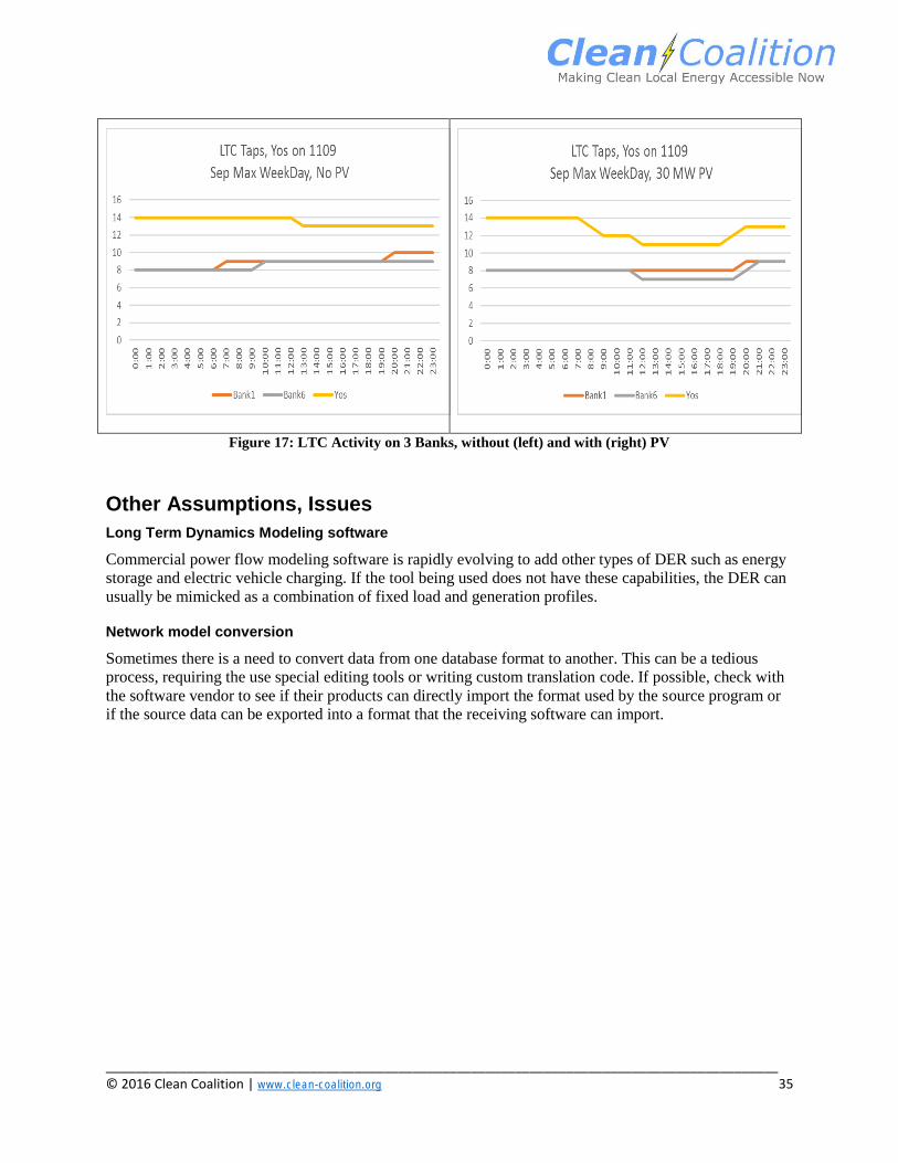
Voltage regulator activity is also important. The timing of state changes can provide insight into how the
regulation is accomplished. Figure 17 shows the increased activity of the LTCs in maintaining voltages
in range.
____________________________________________________________________________________________ © 2016 Clean Coalition | www.clean-coalition.org 35
Figure 17: LTC Activity on 3 Banks, without (left) and with (right) PV
Other Assumptions, Issues
Long Term Dynamics Modeling software
Commercial power flow modeling software is rapidly evolving to add other types of DER such as energy
storage and electric vehicle charging. If the tool being used does not have these capabilities, the DER can
usually be mimicked as a combination of fixed load and generation profiles.
Network model conversion
Sometimes there is a need to convert data from one database format to another. This can be a tedious
process, requiring the use special editing tools or writing custom translation code. If possible, check with
the software vendor to see if their products can directly import the format used by the source program or
if the source data can be exported into a format that the receiving software can import.
____________________________________________________________________________________________ © 2016 Clean Coalition | www.clean-coalition.org 36
Appendix B: How Adding DG Affects Local Voltage
Adding DER to a grid will increase the voltage locally. The amount of the voltage rise depends on the
magnitude of the DER; the amount and location of loads, reactive power, and other DER; and the
resistance and reactance of the grid itself. The mathematical relationship between the variables is given in
Equation 1 below.
(1)
PL, QL are active and reactive power of the load, respectively, and is the active power of PV,
respectively. PL – PPV is the active power flow and QL the reactive power flow through the feeder.
This equation represents two important features when connecting PV to the distribution grid and
illustrates PV’s impact on the flow of power and voltage profile throughout the feeder. First, as the feeder
becomes saturated with PV, the network will exhibit a reversal of the normal direction of power flow.
Second, the voltage rise in the feeder depends on the feeder resistance (R) and reactance (X). Since R
values are generally much higher than X values, the first term in the numerator, , usually
dominates and the voltage increase is simply a function of the difference in the power consumed by the
load and generated by the PV. In extreme cases, when loads are low and the resistance of the grid is high,
the added PV can cause the voltage of the grid to exceed allowed limits, as illustrated in Figure 5. In
order to prevent this from occurring, PV should be installed in as close proximity to loads as possible.
References CPUC DRP. (n.d.). Distribution Resources Plan (R.14-08-013). Retrieved from
http://www.cpuc.ca.gov/General.aspx?id=5071
Jennifer Taylor, C. H. (2009). Basics of Load Allocation. Retrieved from Slideshare.net:
http://www.slideshare.net/MilsoftUtilitySolutions/basics-of-load-allocation-jennifer-taylor-and-
chris-hammond
Milsoft. (n.d.). Engineering Analysis and Load Allocation. Retrieved from Milsoft.com:
http://www.milsoft.com/sites/www.milsoft.com/files/presentation-files/2011%20-
%20Engineering%20Analysis%20&%20Load%20Allocation.pdf
Wikipedia. (n.d.). Power-flow study. Retrieved from wikipedia.org: https://en.wikipedia.org/wiki/Power-
flow_study