1

Humanoid Robotics

Inverse Kinematics and Whole-Body Motion Planning

Maren Bennewitz

2

Motivation §  Plan a sequence of configurations (vector of

joint angle values) that let the robot move from its current configuration to a desired goal configuration

§  High-dimensional search space according to the degrees of freedom of the humanoid

§  Several constraints have to be considered such as joint limits, avoidance of self- and obstacle collisions, and balance

3

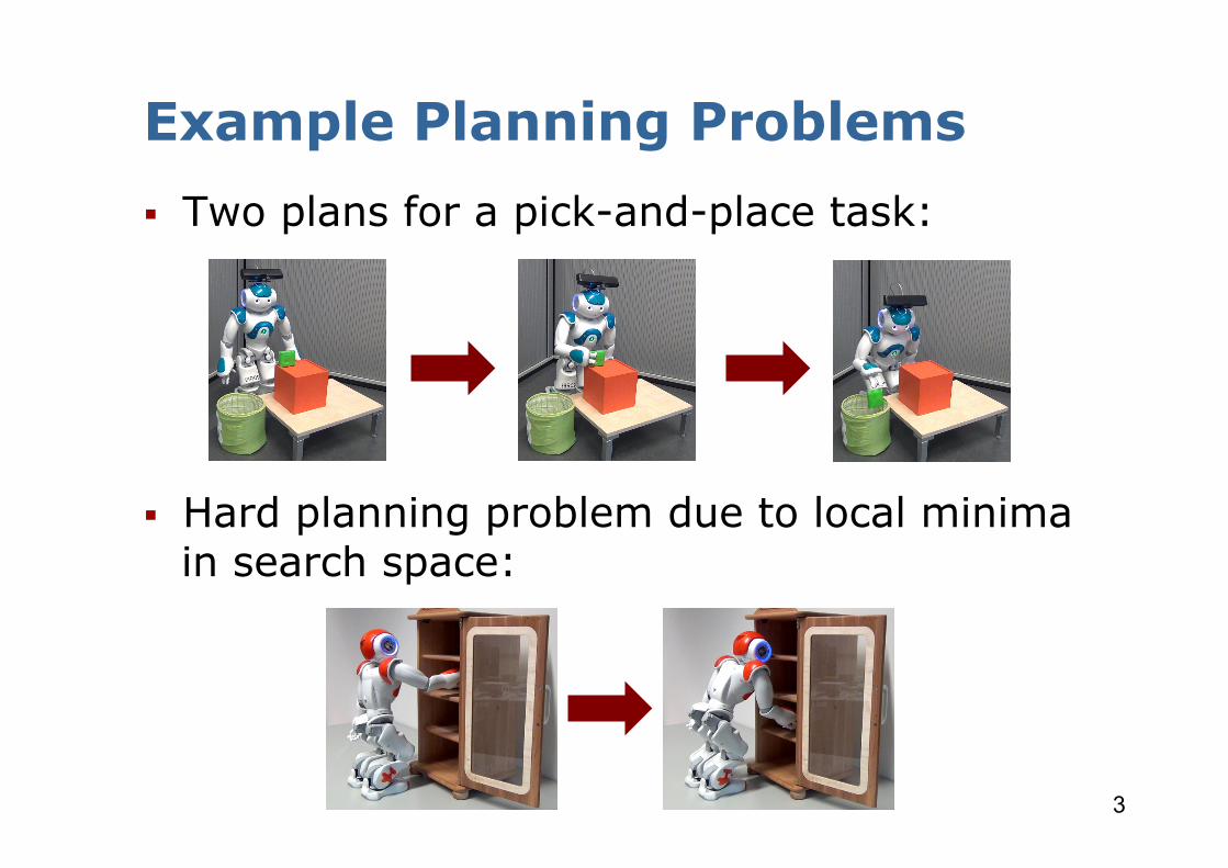
Example Planning Problems §  Two plans for a pick-and-place task:

§  Hard planning problem due to local minima in search space:

4

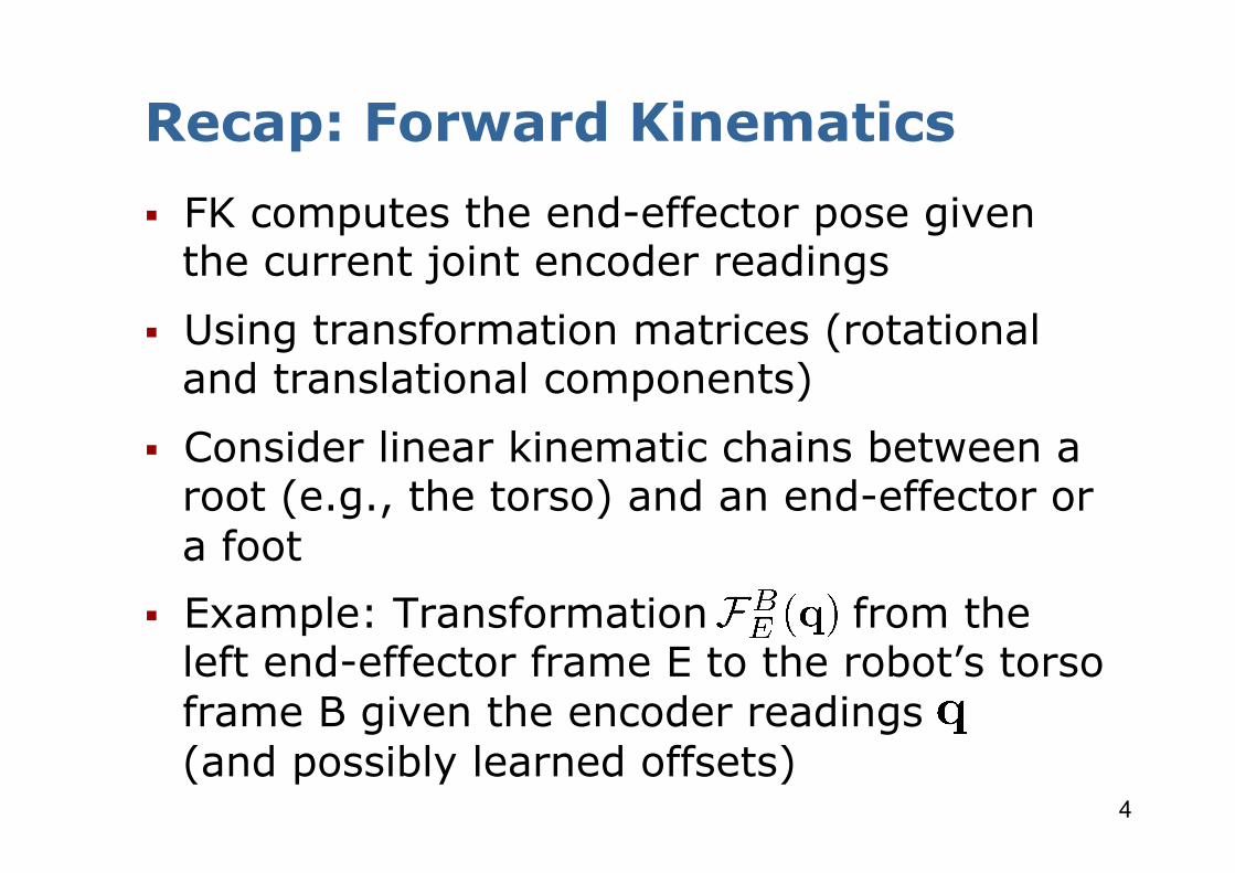
Recap: Forward Kinematics §  FK computes the end-effector pose given

the current joint encoder readings §  Using transformation matrices (rotational

and translational components) §  Consider linear kinematic chains between a

root (e.g., the torso) and an end-effector or a foot

§  Example: Transformation from the left end-effector frame E to the robot’s torso frame B given the encoder readings (and possibly learned offsets)

5

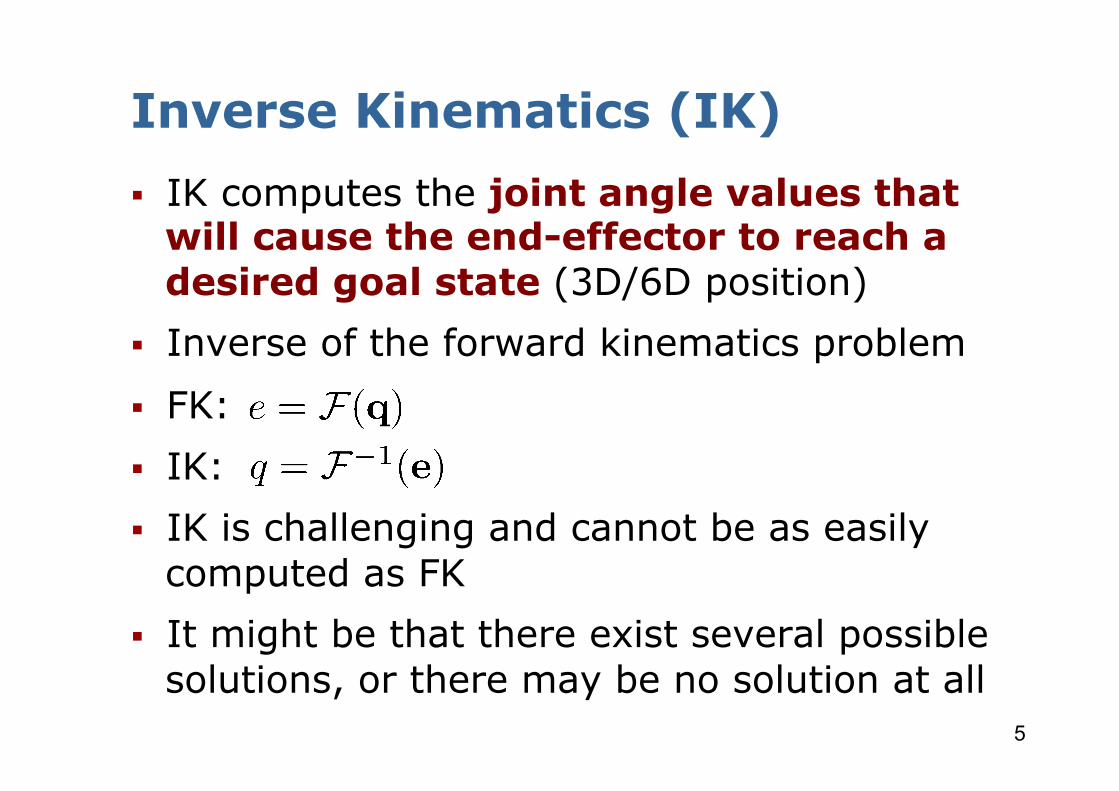
Inverse Kinematics (IK) §  IK computes the joint angle values that

will cause the end-effector to reach a desired goal state (3D/6D position)

§  Inverse of the forward kinematics problem §  FK: §  IK: §  IK is challenging and cannot be as easily

computed as FK §  It might be that there exist several possible

solutions, or there may be no solution at all

6

Inverse Kinematics (IK) §  Even if a solution exists, it may require

complex computations to find it §  Many different approaches to solving IK

problems exist §  Analytical methods: Closed-form solution,

directly invert the forward kinematics equations, use trig/geometry/algebra

§  Numerical methods: Use approximation and iteration to converge to a solution, usually more expensive but also more general

7

Inverse Kinematics Solver §  IKFast: Analytically IK, very fast,

calculates all possible solutions http://openrave.org/docs/latest_stable/openravepy/ikfast/

§  Kinematics and Dynamics Library (KDL): Included in ROS, contains several numerical methods for IK http://wiki.ros.org/kdl

8

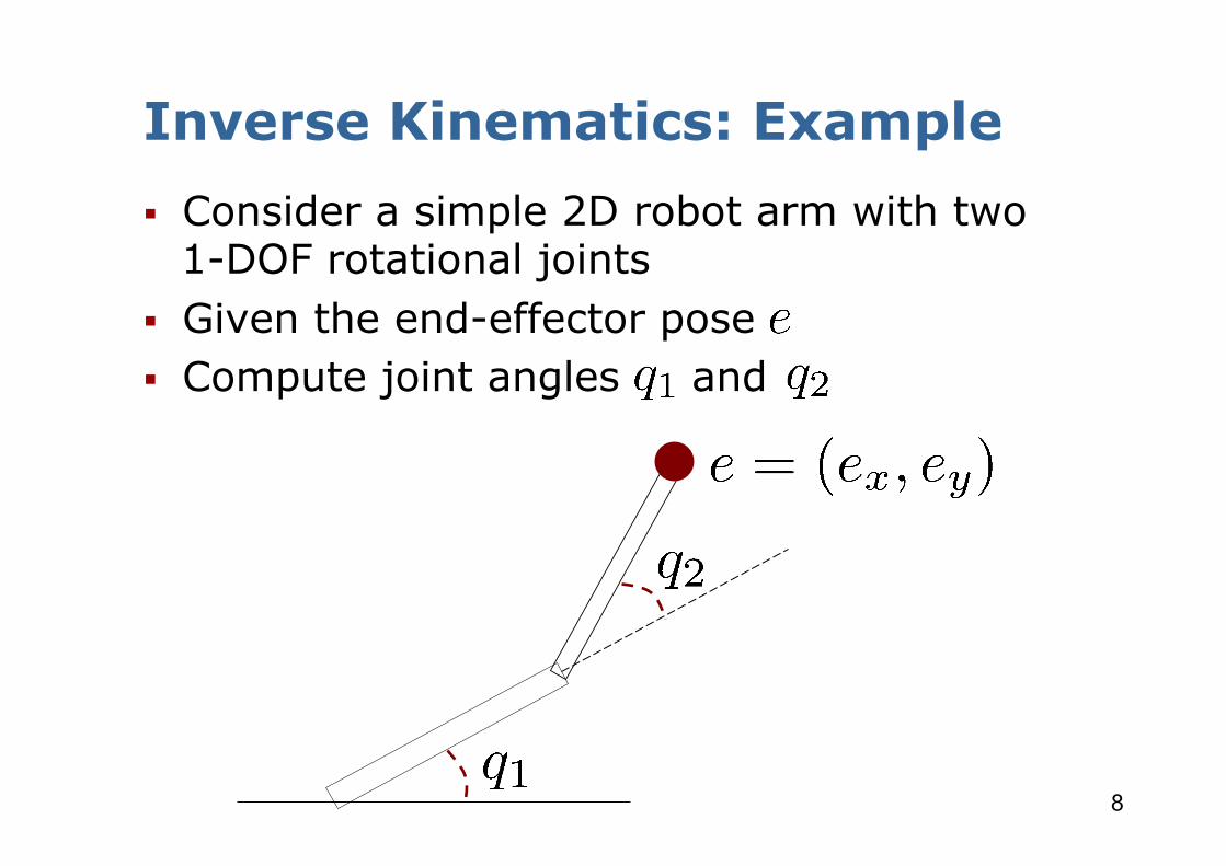
Inverse Kinematics: Example §  Consider a simple 2D robot arm with two

1-DOF rotational joints §  Given the end-effector pose §  Compute joint angles and

9

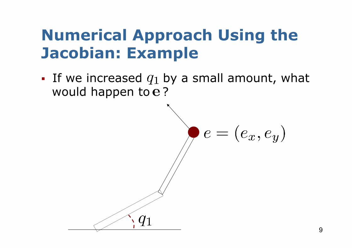
Numerical Approach Using the Jacobian: Example §  If we increased by a small amount, what

would happen to ?

10

Numerical Approach Using the Jacobian: Example §  If we increased by a small amount, what

would happen to ?

11

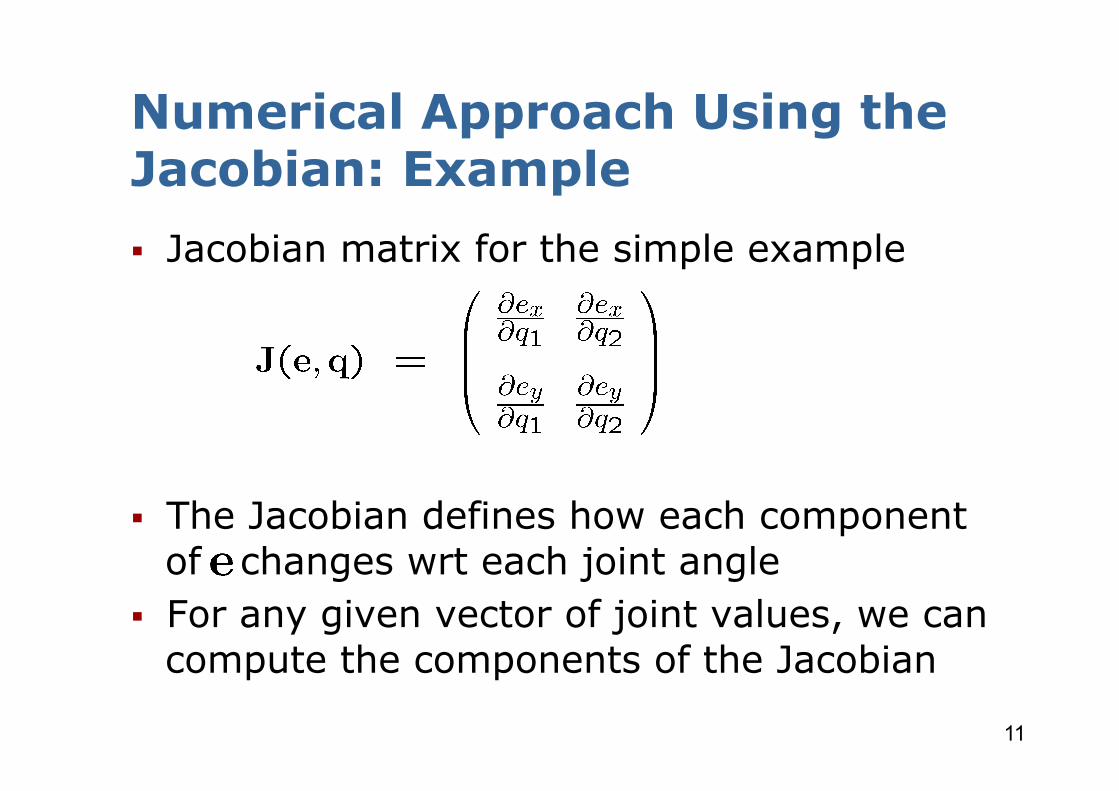
Numerical Approach Using the Jacobian: Example §  Jacobian matrix for the simple example

§  The Jacobian defines how each component of changes wrt each joint angle

§  For any given vector of joint values, we can compute the components of the Jacobian

12

Numerical Approach Using the Jacobian §  In general, the Jacobian will be an 3xN or

6xN matrix where N is the number of joints §  For each joint, analyze how would change

if the joint position changed §  The Jacobian can be computed based on the

equation of FK

13

Numerical Approach Using the Jacobian §  Given a desired incremental change in the

end-effector configuration, we can compute an appropriate incremental change in joint DOFs:

§  As cannot be inverted in the general case,

it is replaced by the pseudoinverse or by the transpose in practice (see KDL library)

14

Numerical Approach Using the Jacobian §  Forward kinematics is a nonlinear function

(as it involves sin’s and cos’s of the input variables)

§  Thus, we have an approximation that is only valid near the current configuration

§  We must repeat the process of computing the Jacobian and then taking a small step towards the goal until the end-effector is close to the desired pose

15

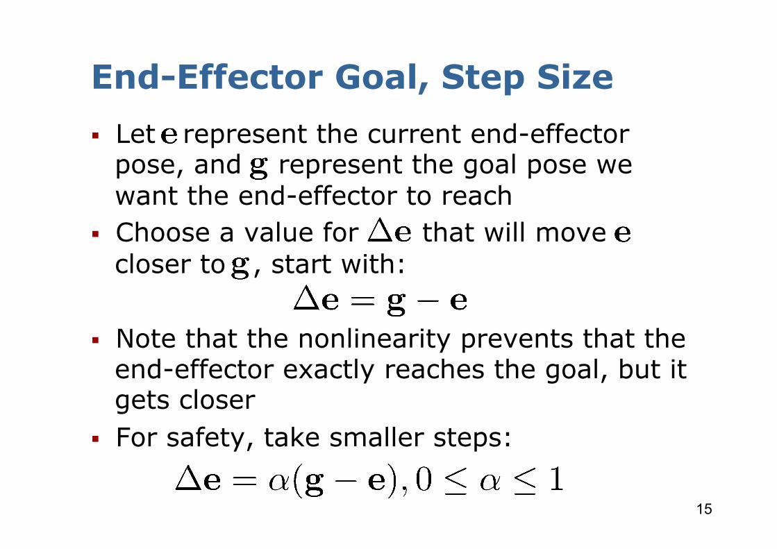
End-Effector Goal, Step Size §  Let represent the current end-effector

pose, and represent the goal pose we want the end-effector to reach

§  Choose a value for that will move closer to , start with:

§  Note that the nonlinearity prevents that the

end-effector exactly reaches the goal, but it gets closer

§  For safety, take smaller steps:

16

Basic Jacobian IK Technique while ( is too far from ) { Compute for the current config. Compute // choose a step to take // compute change in joints

// apply change to joints Compute resulting // apply FK compute new pose of end-effector

}

17

Limitations of the IK-based Approach §  For local motion generation problems, IK-

based methods can be applied §  Numerical optimization methods, however,

bear the risk of being trapped in local minima

§  For more complex problems requiring collision-free motions in narrow environments, planning methods have to be applied

18

Whole-Body Motion Planning §  Find a path through a high-dimensional

configuration space (>20 dimensions) §  Consider constraints such as avoidance of

joint limits, self- and obstacle collisions, and balance

§  Complete search algorithms are not tractable

§  Apply a randomized, sampling-based approach to find a valid sequence of configurations

19

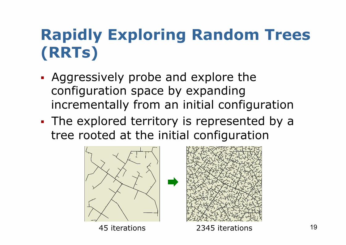
Rapidly Exploring Random Trees (RRTs) §  Aggressively probe and explore the

configuration space by expanding incrementally from an initial configuration

§  The explored territory is represented by a tree rooted at the initial configuration

45 iterations 2345 iterations

20

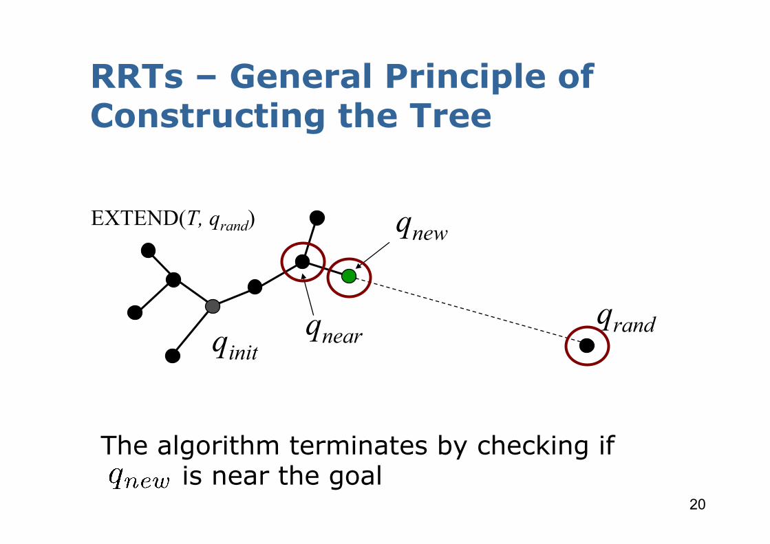
RRTs – General Principle of Constructing the Tree

RI 16-735, Howie Choset with slides from James Kuffner

Path Planning with RRTs(Rapidly-Exploring Random Trees)

BUILD_RRT (qinit) {T.init(qinit); for k = 1 to K do

qrand = RANDOM_CONFIG(); EXTEND(T, qrand)

}

EXTEND(T, qrand)

qnear

qnew

qinitqrand

[ Kuffner & [ Kuffner & LaValleLaValle , ICRA, ICRA’’00]00]

The algorithm terminates by checking if is near the goal

21

Bias Towards Goal §  When expanding, with some probability

(5-10%) pick the goal instead of a random node

§  Why not picking the goal every time? §  This will waste much effort in running into

local minima (due to obstacles or other constraints) instead of exploring the space

22

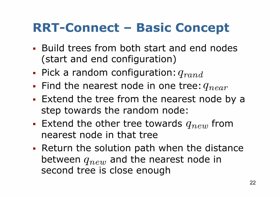
RRT-Connect – Basic Concept §  Build trees from both start and end nodes

(start and end configuration) §  Pick a random configuration: §  Find the nearest node in one tree: §  Extend the tree from the nearest node by a

step towards the random node: §  Extend the other tree towards from

nearest node in that tree §  Return the solution path when the distance

between and the nearest node in second tree is close enough

23

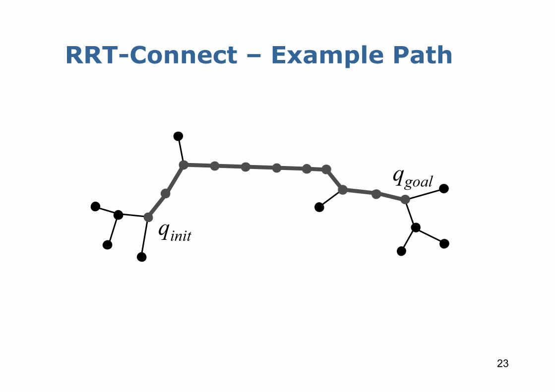
RRT-Connect – Example Path

RI 16-735, Howie Choset with slides from James Kuffner

qinit

qgoal

7) Return path connecting start and goal

24

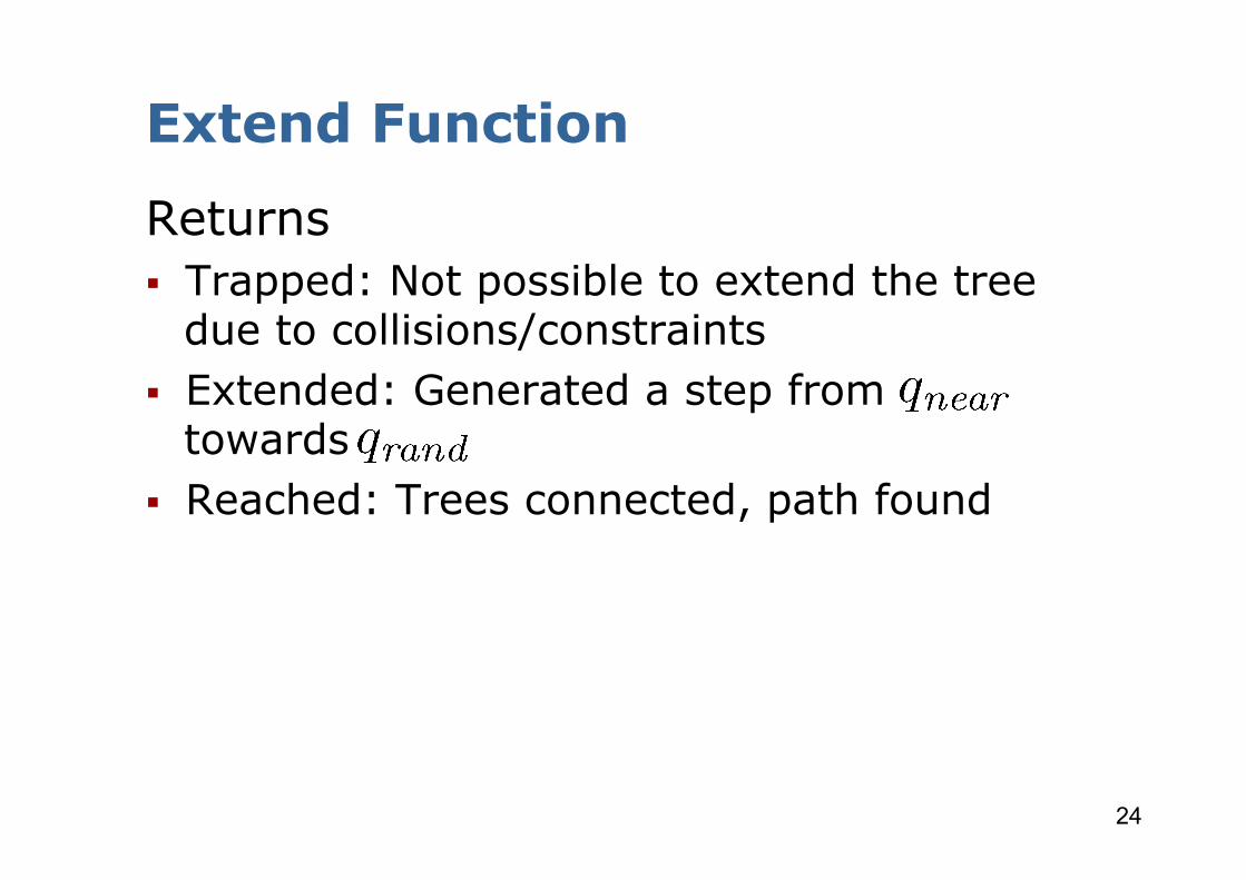
Extend Function

Returns §  Trapped: Not possible to extend the tree

due to collisions/constraints §  Extended: Generated a step from

towards §  Reached: Trees connected, path found

25

RRT-Connect

RI 16-735, Howie Choset with slides from James Kuffner

Basic RRT-Connect

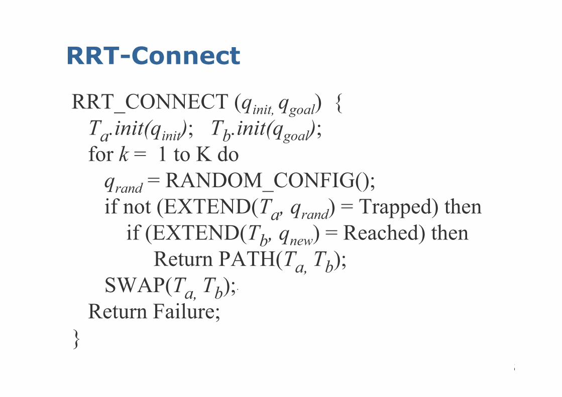
RRT_CONNECT (qinit, qgoal) {Ta.init(qinit); Tb.init(qgoal); for k = 1 to K do

qrand = RANDOM_CONFIG(); if not (EXTEND(Ta, qrand) = Trapped) then

if (EXTEND(Tb, qnew) = Reached) thenReturn PATH(Ta, Tb);

SWAP(Ta, Tb);Return Failure;

}

Instead of switching, use Ta as smaller tree. This helped James a lot

26

RRTs – Properties (1) §  Easy to implement §  Fast §  Produce non-optimal paths: Solutions are

typically jagged and may be overly long §  Post-processing such as smoothing

smoothing is necessary: Connect non-adjacent nodes along the path with a local planner

§  Generated paths are not repeatable and unpredictable

§  Rely on a distance metric (e.g., Euclidean)

27

RRTs – Properties (2) §  Probabilistic completeness:

The probability of finding a solution if one exists approaches one

§  However, when there is no solution (path is blocked due to constraints), the planner may run forever

§  To avoid endless runtime, the search is stopped after a certain number of iterations

28

Considering Constraints for Humanoid Motion Planning §  When randomly sampling configurations,

most of them will not be valid since they cause the robot to lose its balance

§  Use a set of precomputed statically stable double support configurations from which we sample

§  Check for joint limits, self-collision, collision with obstacles, and whether it is statically stable within the extend function

29

Collision Checking §  FCL library for collision checks

https://github.com/flexible-collision-library/fcl

§  Check the mesh model of each robot for self-collisions and collisions with the environment

30

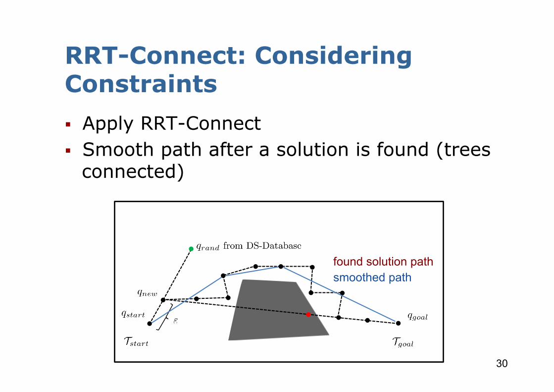
RRT-Connect: Considering Constraints §  Apply RRT-Connect §  Smooth path after a solution is found (trees

connected)

f  

found solution path smoothed path

31

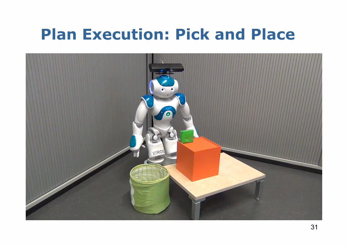
Plan Execution: Pick and Place

32

Plan Execution: Grabbing Into a Cabinet

33

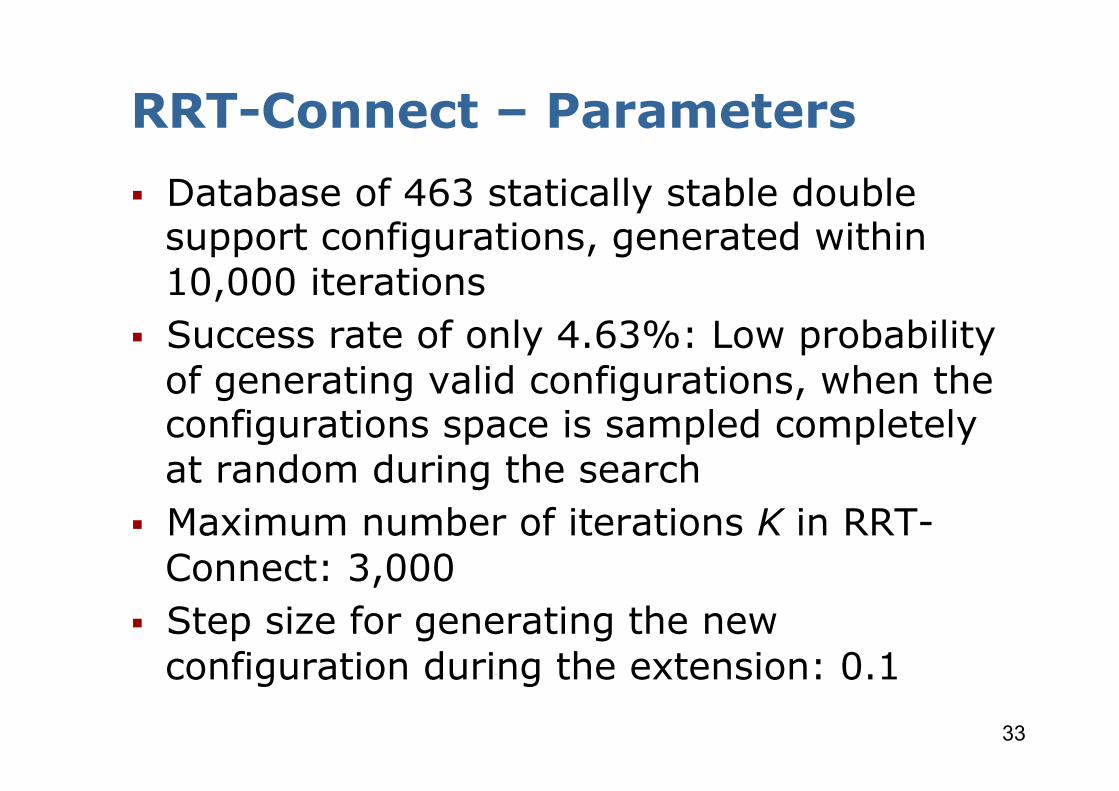
RRT-Connect – Parameters §  Database of 463 statically stable double

support configurations, generated within 10,000 iterations

§  Success rate of only 4.63%: Low probability of generating valid configurations, when the configurations space is sampled completely at random during the search

§  Maximum number of iterations K in RRT-Connect: 3,000

§  Step size for generating the new configuration during the extension: 0.1

34

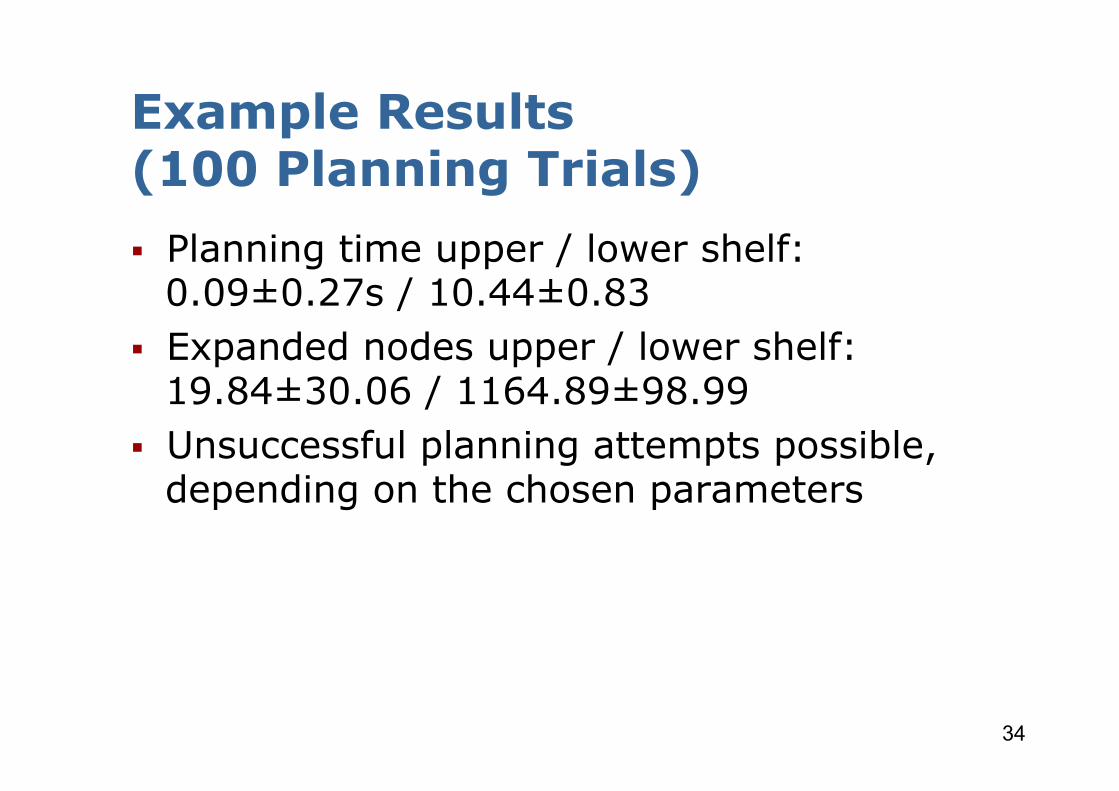
Example Results (100 Planning Trials) §  Planning time upper / lower shelf:

0.09±0.27s / 10.44±0.83 §  Expanded nodes upper / lower shelf:

19.84±30.06 / 1164.89±98.99 §  Unsuccessful planning attempts possible,

depending on the chosen parameters

35

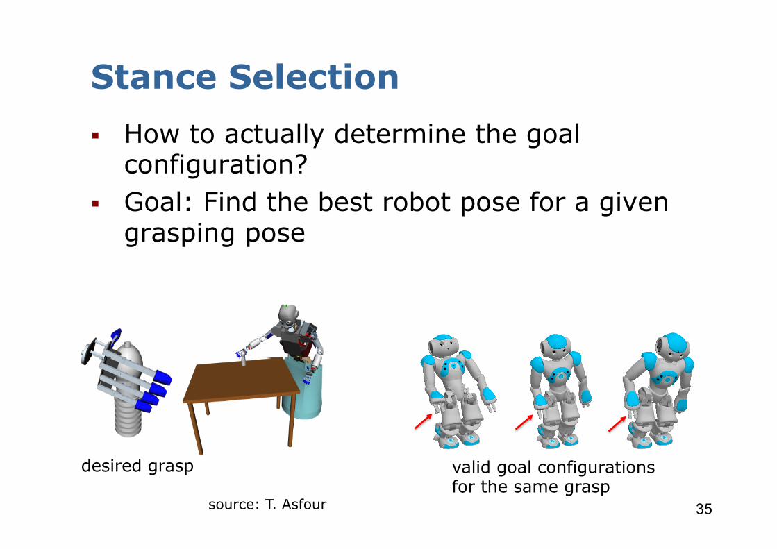
Stance Selection §  How to actually determine the goal

configuration? §  Goal: Find the best robot pose for a given

grasping pose

source: T. Asfour

desired grasp valid goal configurations for the same grasp

36

Spatial Distribution of the Reachable End-Effector Poses

§  Representation of the robot’s reachable workspace

§  Data structure generated in an offline step: reachability map (voxel grid)

§  Represents all possible end-effector poses and quality information (manipulability)

37

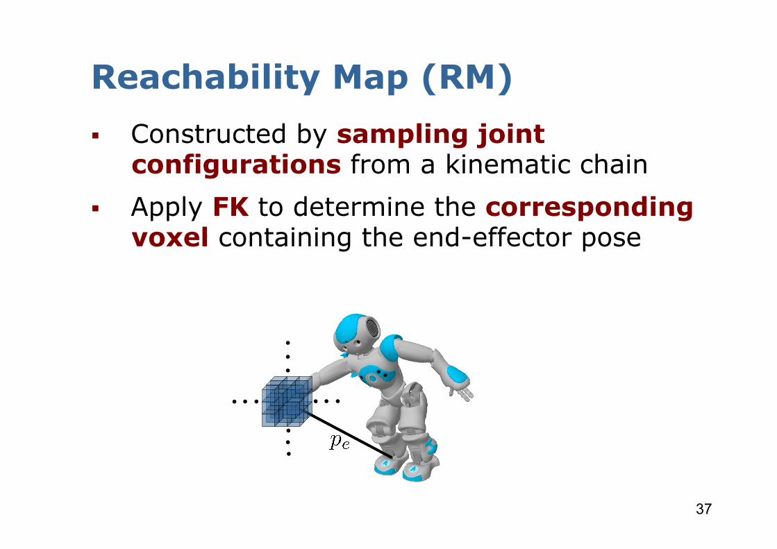
Reachability Map (RM) §  Constructed by sampling joint

configurations from a kinematic chain §  Apply FK to determine the corresponding

voxel containing the end-effector pose

38

Reachability Map (RM) §  Constructed by sampling joint

configurations from a kinematic chain §  Apply FK to determine the corresponding

voxel containing the end-effector pose §  Configurations are added to the RM if they

are statically-stable and self-collision free §  Result: Reachability representation, each

voxel contains configurations and quality measure

§  Generating the RM is time-consuming, but done only once offline

39

Configuration Sampling §  Stepping though the range of the

kinematic chain’s joints §  Serial chain: joints between the

right foot and the gripper link §  Larger step width for the upper

body joints to keep the reachability map representation sparse

§  Smaller step width for the lower body joints to increase the probability of achieving a double support configuration

40

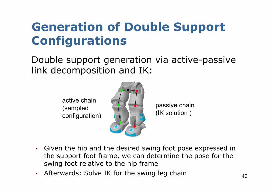
Generation of Double Support Configurations Double support generation via active-passive link decomposition and IK:

active chain (sampled configuration)

passive chain (IK solution )

§  Given the hip and the desired swing foot pose expressed in the support foot frame, we can determine the pose for the swing foot relative to the hip frame

§  Afterwards: Solve IK for the swing leg chain

41

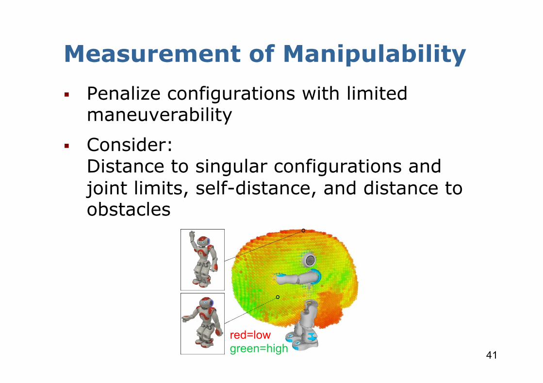
Measurement of Manipulability §  Penalize configurations with limited

maneuverability §  Consider:

Distance to singular configurations and joint limits, self-distance, and distance to obstacles

red=low green=high

42

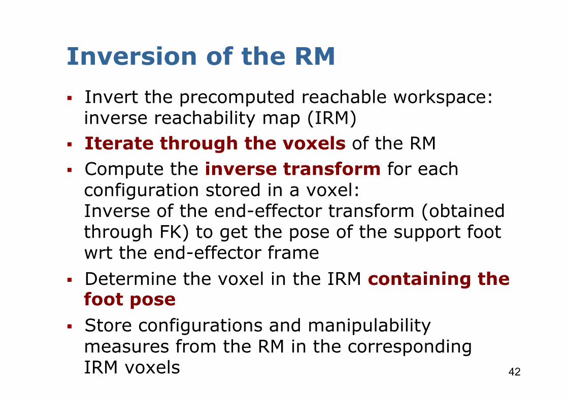
Inversion of the RM §  Invert the precomputed reachable workspace:

inverse reachability map (IRM) §  Iterate through the voxels of the RM §  Compute the inverse transform for each

configuration stored in a voxel: Inverse of the end-effector transform (obtained through FK) to get the pose of the support foot wrt the end-effector frame

§  Determine the voxel in the IRM containing the foot pose

§  Store configurations and manipulability measures from the RM in the corresponding IRM voxels

43

Inversion of the RM Algorithm 2: Reachability Map Inversion (RM )

1 while v GET VOXEL(RM ) do2 n

c

GET NUM CONFIGS(v)3 for i = 1 to n

c

do4 (q

c

, q

SWL

, w) GET CONFIG DATA(v, i)5 p

tcp

COMPUTE TCP POSE(qc

)6 p

base

(ptcp

)�1

7 idx FIND EE VOXEL(pbase

)8 IRM ADD CONF TO VOXEL(idx, q

c

, q

SWL

, w)9 end

10 end

its extend from a statically stable and collision-free doublesupport configuration. Since sampling is performed onlyfor a serial chain of the robot, e.g., for the joint betweenthe foot and gripper link, the loop-closure and stabilityconstraint must be additionally enforced. The former requiresthe adaption of the swing leg configuration such that the feetof the robot are placed parallel to each other on the floor.Here, we apply the active-passive link decomposition methodintroduced in [12] to achieve a closed-loop configuration forthe leg, where the active chain is the support leg for whichjoint values are sampled and the passive chain is the swingleg. Let us assume w.l.o.g that the right leg is the supportleg whose configuration is given by q

SUL

(Line 3 of Alg. 1).By computing the forward kinematics we obtain the posep

hip

of the hip frame Fhip

w.r.t. the support foot frameF

rfoot

(see Fig. 2). Then, using the fixed transformationp

SUF

SWF

expressing the desired pose of the swing foot frameF

lfoot

w.r.t. the support foot we can infer the desired posep

SWF

of the swing foot w.r.t. frame Fhip

. We then applyan inverse kinematics solver to find a configuration for theswing leg q

SWL

.

V. REACHABILITY MAP INVERSION

The reachability map generated according to Sec. IV rep-resents the robot’s capability of reaching certain end-effectorposes from statically stable, collision-free double supportconfigurations. In manipulation and reaching tasks, however,we face exactly the inverse problem. Namely, the requiredend-effector pose is predefined by the pose of an object to begrasped and we aim at finding a base or feet configurationthat maximizes the probability of successful task execution.For this purpose, we use an inverse reachability map (IRM)that represents potential base or feet poses relative to the end-effector. The IRM is generated by inverting the previouslygenerated reachability map. The individual steps performedfor inverting the reachability information are shown aspseudo code in Alg. 2 and will be explained in detail inthe following.

Given the reachability map RM as input, we iteratethrough its voxels v and for each of them in turn through then

c

configurations stored in it (Line 1 of Alg. 2). Here, the i-thconfiguration of voxel v is represented by the data structurecomposed of the configuration of the sampled chain q

c

, theconfiguration of the swing leg q

SWL

and the manipulabilitymeasure w (Line 4 of Alg. 2). By computing the inverseof the end-effector transformation p

tcp

, obtained by solving

Fig. 3: Cross section through the IRM showing potentialright foot locations (left foot is parallel) relative to the handof the robot. Voxels are colored by their manipulabilityindex (red = low, green = high).

the forward kinematics for the sampled chain, we obtainthe pose p

base

of the support foot w.r.t. the end-effectorframe (Line 5, 6 of Alg. 2). Equivalent to the reachabilitymap construction in Alg. 1, we afterwards determine theindex idx of the IRM voxel containing the support footin pose p

base

and add the configuration to the inverse reach-ability map data structure (Line 7, 8 of Alg. 2). Note that themap inversion process does not invalidate any configurationsof the RM . Thus, no additional check for constraint violationis required. The generated IRM is representing a set ofvalid stance poses relative to the end-effector independentfrom any specific grasp configuration. A cross section of anIRM , representing all right foot poses w.r.t. the right gripperis shown in Fig. 3. As with the RM , the IRM needs to bebuilt only once in an offline step and can subsequently beused in all stance pose selection queries for required targetgrasp poses.

VI. SELECTING STANCE POSES USING THE INVERSEREACHABILITY MAP (IRM)

Once the IRM has been computed, it can be used todetermine the optimal stance pose for a given grasping pose.Here, we assume a 6D target pose for the end-effector givenas

p

global

grasp

= (x, y, z, roll, pitch, yaw)T , (3)

where (x, y, z)T and (roll, pitch, yaw)T is the position andorientation of the desired grasp pose w.r.t. the global frameF

global

. To obtain the set of potential stance poses for aspecific grasp pose from the IRM , we perform the followingsteps (see also Alg. 3). At first, the IRM is transformed inorder to align its center with the grasp frame F

grasp

(Line 1of Alg. 3). Afterwards, we determine the intersection ofthe transformed map IRM

grasp

with the ground plane onwhich the feet must be placed planar (Line 2 of Alg. 3). Theresulting layer IRM

floor

of ground floor voxels representsall support foot positions from which the grasp pose pglobal

grasp

isreachable. However, the orientation of the support foot poses

configuration of sampled chain configuration of the swing leg

end-effector pose via FK inverse of transform to get pose of the foot wrt EE frame

determine voxel of support foot

The IRM represents valid stance poses relative to the end-effector

manipulability measure

44

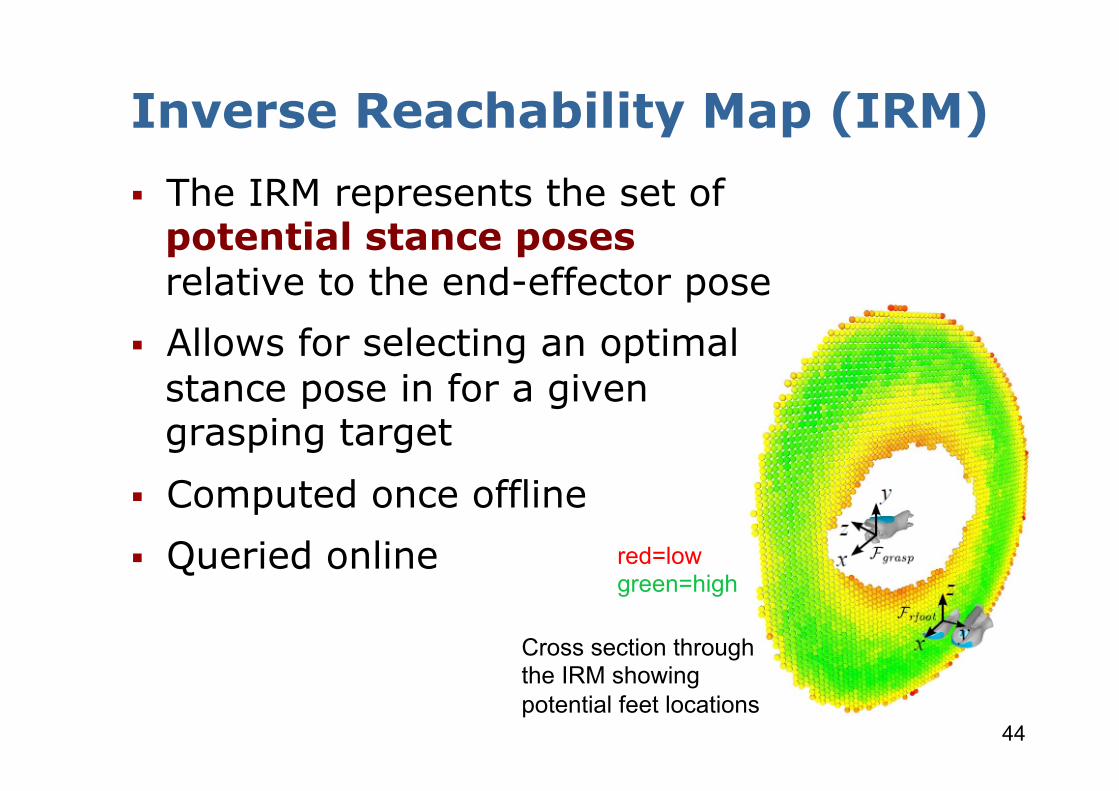
Inverse Reachability Map (IRM) §  The IRM represents the set of

potential stance poses relative to the end-effector pose

§  Allows for selecting an optimal stance pose in for a given grasping target

§  Computed once offline §  Queried online

Cross section through the IRM showing potential feet locations

red=low green=high

45

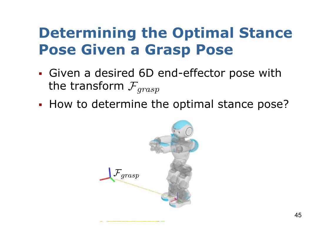
Determining the Optimal Stance Pose Given a Grasp Pose §  Given a desired 6D end-effector pose with

the transform §  How to determine the optimal stance pose?

46

Determining the Optimal Stance Pose Given a Grasp Pose §  The IRM needs to be transformed and valid

configurations of the feet on the ground have to be determined

§  Transform the IRM voxel centroids according to to get

§  Intersect with the floor plane F:

§  Remove unfeasible configurations from to get

47

Determining the Optimal Stance Pose: Example

desired grasp pose

optimal stance pose

Select the optimal stance pose from the voxel with the highest manipulability measure

red=low green=high

48

Summary (1) §  IK computes the joint angle values so that

the end-effector reaches a desired goal §  Several analytical/numerical approaches §  Basic Jacobian IK technique iteratively

adapts the joint angles to reach the goal §  Motion planning: Computes global plan from

the initial to the goal configuration §  RRTs are efficient and probabilistically

complete, but yield non-optimal, not repeatable, and unpredictable paths

49

Summary (2) §  RRTs have solved previously unsolved

problems and have become the preferred choice for many practical problems

§  Several extensions exist, e.g., anytime RRTs §  Also approaches that combine RRTs with

local Jacobian control methods have been proposed

§  Efficiently determine the optimal stance pose for a given grasping pose using an IRM that is computed once offline

50

Literature (1) §  Introduction to Inverse Kinematics with Jacobian

Transpose, Pseudoinverse and Damped Least methods S.R. Buss, University of California, 2009

§  RRT-Connect: An Efficient Approach to Single-Query Path Planning J. Kuffner and S. LaValle , Proc. of the IEEE International Conference on Robotics & Automation (ICRA), 2000

§  Whole-Body Motion Planning for Manipulation of Articulated Objects F. Burget, Armin Hornung, and M. Bennewitz, Proc. of the IEEE International Conference on Robotics & Automation (ICRA), 2013

51

Literature (2) §  Stance Selection for Humanoid Grasping Tasks by

Inverse Reachability Maps F. Burget and M. Bennewitz, Proc. of the IEEE International Conference on Robotics & Automation (ICRA), 2015

§  Robot Placement based on Reachability Inversion N. Vahrenkamp, T. Asfour, and R. Dillmann, Proc. of the IEEE International Conference on Robotics & Automation (ICRA), 2013

52

Acknowledgment §  Parts of the slides rely on presentations of

Steve Rotenberg, Kai Arras, Howie Choset, and Felix Burget