Human Pose Extraction from Monocular Videosusing Constrained Non-Rigid Factorization

Appu ShajiDept. of Computer Science and Engineering

IIT Bombay

Powai, Mumbai 400 076, India

appu@cse.iitb.ac.in

Behjat SiddiquieDept. of Computer Science

University of Maryland

College Park, MD 20742, USA

behjat@cs.umd.edu

Sharat ChandranDept. of Computer Science and Engineering

IIT Bombay

Powai, Mumbai 400 076, India

sharat@cse.iitb.ac.in

David SuterDept. of Electrical and Computer Systems Engineering

Monash University

Clayton 3800, Victoria, Australia

d.suter@eng.monash.edu.au

Abstract

We focus on the problem of automatically extracting the 3D configuration of humanposes from 2D image features tracked over a finite interval of time . This problemis highly non-linear in nature and confounds standard regression techniques. Ourapproach effectively marries a non-rigid factorization algorithm with prior learnedstatistical models from archival motion capture database. We show that a stand alonenon-rigid factorization algorithm is highly unsuitable for this problem. However,when coupled with the learned statistical model in the form of a constrained non-linear programming method, it yields a substantially better solution.

1 IntroductionGiven a monocular video which features a single human in motion, our goal in this work is to re-construct the 3D configuration (seen from an arbitrary choice of a world coordinate system). Weassume that we have as input anatomically well-defined landmark points (such as major joints)recorded from an orthographic or weak-perspective camera. Our emphasis is not in feature track-ing, but rather on recovering the lost depth during image formation from noisy and possiblyincomplete data.

Human motion comprises of an enormous amount of inherent subtlety and variability. Conse-quently the problem of inferring 3D pose from 2D image sequences is highly non-linear in natureand confounds standard regression techniques. Besides, even if we have a good knowledge aboutthe projection matrix of the camera, for any single input observation of a human pose in 2D, thereare possibly multiple valid body configurations. Correlate this with our lack of judgment whenwe see the Necker cube. From a numerical point of view, estimating 3D structure and motionfrom image sequences is a higher order (quartic) non-linear optimization problem (§Eq. 5), proneto local minima. These local minima are intrinsic to the problem (termed as true illusions [1]).

Previous Work: A variety of statistical as well as deterministic methods have been developedfor extracting pose from single view image sequences. We can define a gross dichotomy onthe class of approaches: Ones that concentrate on learning a mapping from silhouette featurespace to 3D pose [2], and others that try to map feature points, usually localized to anatomicallymeaningful landmark points such as elbows position, limb end-point position etc. to 3D poses [3,4]. Our approach falls in the second category. For a curious reader, we suggest [5] which catalogsmost of the important works on 3D human tracking.

BMVC 2007 doi:10.5244/C.21.92

The solution approach in all of the above cases sans [4] is formulated as an (approximate)probabilistic inference problem. Given an observation, they try to pick a pose from a prior distri-bution which best fits the current likelihood. Though this is an extremely powerful tool, we notethat the methods do not explicitly address geometric properties or algebraic details of the data.Rather, the methods rely on these details being captured during the training stage and appear aslatent parameters. In essence, this transfers too much importance to the training stage.

An alternative less explored, is to borrow techniques from structure from motion (SfM) andcouple them with prior statistical knowledge. SfM [6] techniques are able to produce highlyaccurate solution when the object is rigid, and is widely regarded as one of biggest success storyof computer vision. But, extending SfM to non-rigid scenario has turned out to be quite tricky.One popular flavor of SfM algorithm is the Factorization algorithm [7–10].

In this work, we use a variant of recently proposed [10] non-rigid factorization method (NRF,hereafter) for performing SfM.

Methodology: Factorization methods attempt to capture the implicit geometric invariantspresent in a wide temporal window of input data. (An example invariant might be that two fea-ture points from a single rigid body should have similar motion trajectories. These invariantsuncover themselves as reduced rank constraints [7, 8, 10] on the data observation matrix consist-ing of stacked (x,y) points. This matrix can be factorized into two matrices, one representingthe rotation, and the other representing the shape of the object. A straightforward Singular ValueDecomposition (SVD) of this matrix results in the recovery of this factorization only up-to a gen-eralized linear corrective transform (§Eq. 3). Solving this linear transform is a non-trivial taskfor several reasons as has been recently observed in the literature.

Further, the current factorization based solutions are not directly adaptable to the humanmovement problem (our interest) since the quality of the solution degenerates very rapidly whenthe “deformations” are large1 .

Contribution: In this paper we propose a novel constrained factorization algorithm, whicheffectively couples prior learned statistical knowledge about human shape variability (and the sub-space it spans) from the ground truth motion capture data, with non-rigid factorization algorithm.Specifically, we make use of motion capture data to build a prior reference pre-shape (§Sec. 3.1). We assume that the recovered shape from the NRF algorithm should be structurally similar tothe reference pre-shape. This is formulated as a constrained non-linear programming problem.These constraints on the structure of shape subspaces reduces the search domain and renders theproblem well-posed (Eq. 6). We provide qualitative and quantitative results to demonstrate thevalidity of our scheme.

Notation: We follow the notation used in [10]. a is a scalar, a is a vector and A is a matrix.⊗ denotes Kronecker product. � denotes Hadamard product. vec(A) vectorizes A by stackingits columns and vech(A) vectorizes only its lower triangular portion. A† denotes the generalizedinverse. vc(x,y) = vech(xyT +yxT−diag(x�y)). Note that vc(x,y) operator helps to representequations of the form vec(xTAy) when A is symmetric, more concisely as vc(x,y)T.vech(A)

Road Map In Section 2 we outline two different applications of existing NRF methods, whichare relevant in our context. We first describe how NRF can be used to de-noise and fill in miss-ing entries of a noisy and possibly incomplete data sequence. This is followed up with a briefoverview of a straightforward way of using prior NRF methods, with our experiments that exposessome problems. Section 3 formalizes our notion of shape and describes how shape variability ofan ensemble of data can be captured. Section 4 gives the details of a Sequential Quadratic Pro-gramming based constrained optimization scheme which couples NRF algorithm with the learnedstatistical data. We discuss our experiments and results in Section 5 and conclude in Section 6.

2 Non Rigid FactorizationApart from structure from motion, factorization techniques can be applied to a wide range ofapplication like data segmentation, data de-noising and data imputation. Data de-noising and im-putation are of significant interest to us since the feature tracks from the off-the shelf trackers are

1There has been some recent work on extending factorization methods for articulated structures [11, 12]. But thesemethods require a very large number of features, whereas we work with a very sparse number of features and assume thehuman body to be a deforming object

+ + =︸ ︷︷ ︸R

Figure 1: A pictorial representation of a morphable model. The right hand side is the actual data seen but can be obtained by modifying“basis” shapes.

typically noisy and contain missing information due to occlusion. The de-noising and structurerecovering capability of the factorization algorithm is reviewed in this section.

The Basics: A popular representation for image formation (for either non-rigid or articulatedobjects) under orthographic or weak projective camera models is to write

W f = R f (K

∑i=1

c f iSi)

where W f is the observed 2D feature in frame f (out of F given frames), R f ∈ R2×3 is thetruncated row-orthonormal rotation matrix. K is the number of morph shapes needed to fullyrepresent the object, Si ∈ R3×P the ith morph shapes (where P refers to the number of featurepoints tracked), and c f i, the morph weights corresponding to S in the f th frame. This is pictoriallyrepresented in Fig. 1.

We build an observation matrix W ∈ R2F×P by stacking the position of P landmark pointsobserved in F frames. The structure of the observation matrix W appears in the left hand side ofEq. 1. Here (xi j,yi j) refers to the 2D co-ordinates of the point j in frame i.

P =

x11 · · · x1Py11 · · · y1P... · · ·

...xF1 · · · xFPyF1 · · · yFP

= MS =

cT1 ⊗R1

...cT

F ⊗RF

︸ ︷︷ ︸

2F×3K

S1...

SF

︸ ︷︷ ︸

3K×P

(1)

This factorization can be performed modulo a gauge factor of G ∈ GL(3K,3K) [8](§Sec.2.2)using SVD, if we assume an isotropic and Gaussian noise model2. But when there are outliers andmissing data, which indeed is the case with most real-life measurements due to tracking failureand outliers, a straightforward SVD is no longer applicable.

2.1 Data denoising and missing information recoveryThe most commonly used approach is to re-write the above problem with some robust ρ-functionwhere the contribution of each item is weighted according to its fitness to the subspace [13,14]. The modified factorization problem is now to compute the maximum likely estimator of aweighted L2 norm cost function.

εmle(M, S) = ||W� (P−MS)||2F (2)

where wi j ≥ 0 is a weighing factor which specifies the uncertainty in pi j and wi j = 0 if pi j ismissing

The literature on factorization with missing data falls into several categories: close-form solu-tions, imputation methods, EM-akin alteration methods and direct non-linear minimization meth-ods. An excellent comparative study between these various method can be found in [14].

2Note that though the factorization assumes that temporal dependices in the data are caught by the tracker, the rankconstraint enforces another layer of weak and subtle constraint on the contunity of motion.

(a)

Uncorrupted Data Incomplete and Noisy Data Recovered Data

(b)

Figure 2: Surface and matrix plots (left and right hand side respectively) of noisy+incomplete data, de-noised data and Ground Truth.Notice that the recovered data has a high similarity to the ground truth

Our Denoising Method: We make use of the second order damped Newton algorithm intro-duced in [14] to de-noise the noisy point tracks. But we additionally perform modified Gram-Schmidt orthogonalization on the current estimate of both M and S at each iteration. Note thatEq. 2 does not impose any structure on M or S, whereas SVD based solutions ensured that M andS are orthonormal and form good bases. We find that enforcing the orthonormality at each stepmakes the algorithm more numerically robust, rather than performing one single SVD toward theend. We initialize the optimization with left and right subspace estimate from a sparse SVD [15]of the incomplete data matrix. We weigh the visible features isotropically. These weights areestimated by contrasting the singular value spectrum of the sparse SVD with the mean value of aprior computed ensemble of spectrum of non-noisy, complete and typical data sets. The featureswhich are not visible are assigned zero weights. A typical example is shown in Fig. 2(a). Thedeep trenches in the top figure corresponds to the missing data feature points. Observe that thesevalleys disappear after the de-noising step (middle figure). Moreover, the recovered data has ahigh similarity to the ground truth (bottom figure).

2.2 Recovering Motion and ShapeAs mentioned earlier, unfortunately this factorization is not unique, but determinable only up to anon-singular linear corrective transformation G as

M = M.G S = G−1.S (3)

where we have the true scaled rotation matrix M and shape matrix S. The heart of the non-linearfactorization algorithm lies in solving for this corrective transform G ∈ GL(3K×3K) as describedbriefly below.

Let xTf and yT

f be the pair of rows in M which gives the projection for frame f . Notice that Mis made up of blocks of 2×3 scaled rotation matrices. Hence rows of each of these 2×3 blocksmust be orthogonal and of equal norm.

xTf y f = 0 (orthogonality constraint)

xTf GGT yf = 0⇒ vc(xf, yf)vech(GGT) = 0xT

f x f = yTf y f ⇒ (x f −y f )T (x f +y f ) = 0 (equal norm constraint)

(x f − y f )T GGT (x f + y f )⇒ vc(xf− yf, xf + yf)vech(GGT) = 0Let L = [vc(xf, yf),vc(xf− yf, xf + yf)]T∀ f and QA = LLT

(4)Note that M1:3 = MG1:3 ∈ R2F×3. It turns out that solving for G1:3 is sufficient to solve for

the rest of G [10]. The vanilla NRF computes G1:3GT1:3 that minimizes the sum squared deviation

from orthogonality in the final motion matrix by least squares solving the system of equationsgiven by

OrthErrQA(G1:3) = vech(G1:3GT1:3)

TQAvech(G1:3GT1:3) (5)

The symmetric matrix G1:3G1:3 is later decomposed to G1:3 by performing a rank-3 EVD (G1:3 =VΛ0.5)

Significantly, it was recently shown [9] that these rotation constraints are not sufficient touniquely solve for the corrective transform G for articulate and non-rigid motions. More specif-ically the general solution of the rotation constraints is GHGT , where H is the summation of anarbitrary block skew symmetric matrix and an arbitrary block scale identity matrix. The culprit be-ing the redundancy in the constraint matrix which leaves the solution to Eq. 5 under-constrained.One way to overcome this ill-posedness is a heuristic scheme proposed by the authors of [9] whereshapes in K frames are assumed to be independent and will act as a set of bases. Unfortunately, ingeneral, this is not a good practice, since it tries to represent the shape space non-parsimoniouslywith a finite set of local diffeomorphisms, and hence has questionable subspace representationability [16].

An alternative appears in [10] where Brand makes another relevant observations that approxi-mation of Eq. 5 as a nested linear least square solution doesn’t do justice to the physical reality. Itoverlooks a lot of co-variance information encoded in QA. Instead, the author solves G1:3 directlyfrom Eq. 5 using a variant of first order line search global optimization framework (the step sizesare calculated by direct root finding). But, our experiments showed that the error surfaces gener-ally have a rough terrain and many a times converge to the dreaded local minima. An example isshow in Fig. 3.

Figure 3: Non-rigid factorization algorithms have the tendency to flatten the body structure (notice the legs). The red colored humanmodel is the representation of the actual data and the pink colored model is a reconstruction from 2D data.

The vanilla NRF, does not make any assumption about the shape of the object in scene. But ahuge chunk of vision related engineering problems (in our case human pose extraction) do allowus to make valid assumption regarding object shape subspaces and possibly get an estimate of thesubspace apriori. In the next section we describe how a good prior estimate of shape subspacecan be obtained.

3 Shape AnalysisThe word “shape” is very commonly used in everyday language, usually referring to the appear-ance of an object. Following Kendall [17] the definition of shape that we consider is:

Shape is all the geometrical information that remains when location, scale and rota-tional effects are filtered out from an object

Important aspects of shape analysis are to obtain a measure of distance between shapes, toestimate average shapes from a random sample and to estimate shape variability from a randomsample.

Procrustes analysis involves matching configurations with similarity transformations to be asclose as possible according to Euclidean distance, using least squares techniques. More formally,given two mean centered configuration matrices X1 and X2, the full Procrustes distance betweenX1 and X2 is

Dpro =inf

Γ∈SO(3),β∈R ||Z2−βZ1Γ||

where Xr = Zr/||Xr||,r = 1,2

Similarly, the full Procrustes estimate of mean shape [µ] is obtained by minimizing (over µ)the sum of square full Procrustes distance from each Xi to an unknown unit mean configurationµ , i.e

[µ] = arg infµ

n

∑i=1

d2F(Xi,µ)

For a more detailed exposition, we refer the readers to [18] and the original work of Kendall [17]

3.1 Creating The Reference Pre-ShapeIn the last decade or so, principal component analysis (PCA) has become a favorite tool forcomputer vision and graphics researchers [19, 20]. PCA is a simple, yet powerful technique tocollect and investigate the statistically variability of data which resides in linear spaces (R3 in ourcase). To learn a good set of bases we need a corpus of accurate data with wide variability, whichnow a days is publicly available in the form of archival motion capture data.

Each pose is parametrized as a single observation 60 dimensional column vector (vec(Qtrain))containing the Euclidean positional information of all the land mark points3. We borrow tech-niques from Procrustes Analysis introduced in the previous section to strip these vectors of posi-tional, scale, and orientation details.

If µ be a pre-shape corresponding to the full Procrustes mean shape, the aligned vectors canbe computed as

vF = (1−vec(µ µT))vec(βiQtrainΓi)

These aligned vectors are stacked into a data matrix Xmocap and we compute the principal com-ponents of this data matrix. PCA performs a basis transformation to an orthogonal co-ordinatesystem formed by the eigen vectors Vi of the covariance matrix of Xmocap. These orthogonal com-ponents are ordered with respect to the descending values of their eigenvalues and are arrangedinto Sref. We call Sref as Reference Pre-shape. For a full body motion with just 5 bases we areable to represent more than 94% variation in the data.

4 Constrained FactorizationThe primal idea behind our method is that shapes recovered by the NRF should having significantsimilarity to the pre-learned Reference Pre-Shape. We express this as a constrained non-linearprogramming problem.

More formally, we rewrite Eq. 5 as

E(G1:3) = vech(G1:3GT1:3)

TQAvech(G1:3GT1:3)

S.T trace(G1:3GT1:3) = 1

D2pro(G1:3, SS†

ref)≤−d(6)

where Dpro(X,Y) gives the orthogonal Procrustes distance between X and Y and d is an user-setparameter, which specifies the tolerance level for the structural variation and defines the feasiblearea or the domain of the cost function (smaller the tolerance, narrower the feasible area) . Inour experiments we used 0.2 as the threshold. Though it is tempting to decrease the tolerance,lesser tolerance makes the algorithm more prone to over-fitting (especially if the training set isnot exhaustive enough).

Notice that both our cost function and constraints are non-linear. While the cost function isquartic, the constraints are of quadratic nature. Though constrained non-linear optimization (ingeneral) is still an open problem, many efficient, but approximate numerical schemes exist [21]especially for relatively lower order cost function (quartic, in our case) and near linear constraintfunctions (quadratic). We make use of Sequential Quadratic Programming, a well known andused numerical solution for optimizing smooth non-linear cost functions under smooth non-linearconstraints [21,22]. It is Newton like in that it requires second derivatives of the cost function andpotentially provides quadratic convergence.

The goal is to extremize a scalar cost function E(x) subject to a vector of constraints c(x)≤ 0.(Note that inequality constraints can be treated at par with the equality constraint by assuming its

3Note that the ordering (or the meta-knowledge about it) of this vector has to be consistent with the 2D observationvector.

respective Lagrange multiplier vanishes whenever the inequality is not strict [21] and is strictlypositive whenever the inequality is strict). Lagrange multipliers λ give an implicit solution.

5E +λ 5 c = 0 with c(x) = 0

We resolve this iteratively starting from some initial guess bx0. We approximate the cost tosecond order and the constraints to first order at x0, giving a quadratic optimization sub-problemwith linear constraints.

minδx

(5E.δx+

12

δxT 52 f .δx)|c+5c.δx

This sub-problem has an exact linear solution(52E 5cT

5c 0

)(δxλ

)=−

(5E

c

)(7)

We solve for δx, update x0 to x1 = x0 +δx, re-estimate derivatives and iterate to converge.The first order and second order derivatives of the Lagrange function in Eq. 6 are given in

Appendix A.

5 ExperimentsTraining Data: We use 700 frames from motion capture data included in the HumanEvadataset [5] for learning the pre-shapes. These frames are selected by randomly sampling fromthe training set provided in the dataset. Selected frames span poses from various set of humanaction like walking, boxing, making hand gestures etc.

Testing: We test the performance of our algorithm on synthetic data with ground truth in-cluded in the testing set of the HumanEva dataset, as well as videos which give us only 2Dinformation.

Motion-Capture Based Synthetic Data: In any choice of motion clip (from the motion cap-ture data base) we know the 3D positions. We synthetically created a two dimensional projectionby randomly choosing a center of projection. To simulate tracking errors and the like, the result-ing “features” are further corrupted by adding Gaussian noise and frames dropped randomly tosimulate quantifiable error and occlusion errors in the tracking process. This constituted the pro-cess of creating the observation matrix. The incomplete and noisy observation matrix is denoisedusing the method described in Section 2. Recall that the output of factorization is only accurateup-to an arbitrary rotation and scale. So the error at each frame is defined to be the Procrustesdistance from the recovered orientation to the ground truth. We compare the performance of ouralgorithm to that of the unconstrained case [10].

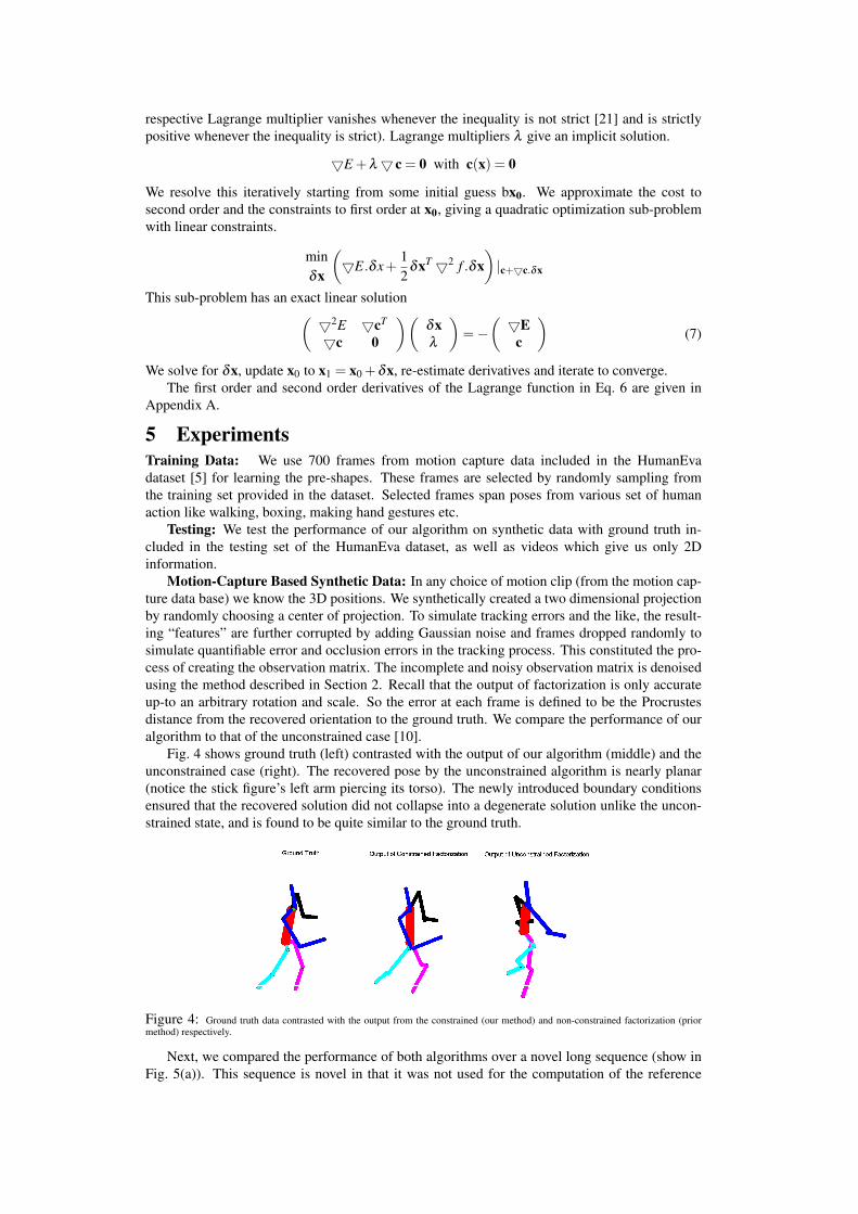
Fig. 4 shows ground truth (left) contrasted with the output of our algorithm (middle) and theunconstrained case (right). The recovered pose by the unconstrained algorithm is nearly planar(notice the stick figure’s left arm piercing its torso). The newly introduced boundary conditionsensured that the recovered solution did not collapse into a degenerate solution unlike the uncon-strained state, and is found to be quite similar to the ground truth.

Figure 4: Ground truth data contrasted with the output from the constrained (our method) and non-constrained factorization (priormethod) respectively.

Next, we compared the performance of both algorithms over a novel long sequence (show inFig. 5(a)). This sequence is novel in that it was not used for the computation of the reference

pre-shape. We selected a complicated clip of a boxing motion consisting of 577 frames sampledat 30Hz. The data is corrupted with 10% additive Gaussian noise and around 15% of its observa-tions are masked out. Note that average performance of the constrained factorization algorithmhovers around the 5–15% reconstruction error mark. One interesting variation in the plot is thatoccasionally (frame numbers 290–320, 348–355 and 380–395) the error of the unconstrained al-gorithm dips somewhat below that of its constrained counter part (our method). The reason forthis unexpected better performance is that during these frames, the actor is assuming a near planarpose and the degenerate shape base extracted by the unconstrained factorization algorithm is bet-ter able to explain these frames. Nevertheless, the unconstrained algorithm rapidly loses accuracyin the more common situation, when the actor resumes his or her flexible movements.

The scatter diagram in Fig. 5(b) plots the average error recorded by the constrained factoriza-tion algorithm (shown in yellow) and its unconstrained counterpart (shown in cyan) for variousdata input (a total of 39 different inputs). Each of the data input was seeded with 2% additiveGaussian error, and no occlusion condition was assumed. While carrying out these experimentswe further assumed that the inequality constraints are strict. Fig. 5(c) shows the performance ofboth the version of the algorithm with three different sequence (walking , boxing and running)when subjected to different amount of synthetic noise. While the dotted line records the perfor-mance of the unconstrained version of the algorithm, the regular line record that of the constrainedone. Walking, Boxing and Dancing motion sequence are represented by the red, green and bluelines respectively. Superior performance by the constrained version of the algorithm is amplyrecorded in every experiment.

0 100 200 300 400 500 6000

0.05

0.1

0.15

0.2

0.25

0.3

0.35

0.4

Pro

cru

stes

Err

or

Frame Number

Unconstrained FactorizationConstrained Factorization

(a) Error comparison of constrained andunconstrained NFM over a 577 frames box-ing sequence

0 5 10 15 20 25 30 35 400

0.02

0.04

0.06

0.08

0.1

0.12

Experiment Number

Aver

age

Angu

lar E

rror

Our MethodBrands Method

(b) Average error of constrained and un-constrained NFM from different experi-ments

0.05 0.1 0.15 0.2 0.25 0.3 0.35 0.4 0.450

0.2

0.4

0.6

0.8

1

1.2

1.4

Amount on Noise (Normalised to 0−1)

Per

cent

age

Err

or

Walking Sequence (our method)

Boxing Sequence (our method)

Dancing Sequnce (our method)

Walking Sequence (Brand’s method)

Boxing Sequence (Brand’s method)

Dancing Sequnce(Brand’s method)

(c) The performance of the algorithm withvarious amount of noise levels

Figure 5: Comparative Performance Evaluation

5.1 Data With No Ground TruthIn this experiment an 80 frame video sequence was semi-automatically tracked using the KLTbased tracker. We hand picked the features which conformed to the anatomically relevant land-mark points. We re-picked the lost features after every 10 frames. Note that far superior trackingschemes exist [23] for tracking humans from video. The purpose of this experiment was to testthe performance under non-linear error models which often appear in real data sequences. Twodifferent ‘pigeon’ views of the recovered orientation of the actor is shown along with actual datais show in Fig. 6. As a post-processing step, the recovered data is smoothed out using a Kalmansmoother. More output including the video of the just explained experiment can be found athttp://www.cse.iitb.ac.in/appu/bmvc07/

6 Conclusion and Future WorkWe have given a novel constrained non-rigid factorization algorithm that extracts 3D human posesfrom 2D video sequences. Both qualitative and quantitative results were provided. Note that ourmethod can be applied to any deforming data sequences (apart from human motion), providedaccurate motion capture or similar high precision quantized data exists.

Future Work: The strength and weakness of factorization based techniques lies in its blockbased nature. This potentially rules out any online scheme. We are currently exploring the pos-sibility of having a windowed scheme, thereby making the algorithm semi-online. We are alsoconsidering having an iterative refinement of reference pre-shape, hence equipping the algorithm

Figure 6: The top row shows the raw frames with features overlayed. The middle and bottom shows the recovered 3d pose renderedfrom two novel view points. The front view is identical and not shown.

to handle non-stationary data, and previously unseen data. Another possibility we wish to exploreis to merge the optimization given in Eq. 2 and Eq. 6 as a single optimization problem.

A DerivativesThe corresponding Lagrange function of Eq. 6 can be written as

L = vech(G1:3GT1:3)

TQAvech(G1:3GT1:3)+λ (vec(G1:3)Tvec(G1:3)−1)

+µ(vec(G1:3− SS†refΓ)Tvec(G1:3− SS†

refΓ)−d) (8)

where Γi ∈ SO(3). Let Z = G1:3 and Ji j ∈ {0,1}3K×3 is all zeros except for element Ji j = 1

∂L (Z,λ ,µ)∂Zi j

=2vech(ZZT)TQAvech(ZJTij +JijZT)+λvec(ZJT

ij +JijZT)

+ µ(vec((Z− SS†refΓ)JT

ij +Jijvec((Z− SS†refΓ)T)

∂L (Z, ,λ ,µ)∂λ

=vec(G1:3)Tvec(G1:3)

∂L (Z, ,λ ,µ)∂ µ

=vec(G1:3− SS†refΓ)Tvec(G1:3− SS†

refΓ)

∂L (Z,λ ,µ)∂ZijZkl

=2.vech(ZJTkl)+JklZT)QA.vech(ZJT

ij +JijZT)

+(vech(ZZT)TQA +λ + µ)vech(JklJTij +JijJT

kl)

(9)

References[1] Soatto, S., Brockett, R.: Optimal structure from motion: Local ambiguites and global estimates. In:

CVPR. (1998) 282–288

[2] Agarwal, A., Triggs, B.: Recovering 3d human pose from monocular images. IEEE Transactions onPattern Analysis & Machine Intelligence 28(1) (2006)

[3] Sigal, L., Black, M.J.: Predicting 3d people from 2d pictures. In: Articulated Motion and DeformableObjects, 4th International Conference. (2006) 185–195

[4] Taylor, C.J.: Reconstruction of articulated objects from point correspondences in a single uncalibratedimage. Computer Vision and Image Understanding 80(3) (2000) 349–363

[5] Sigal, L., Black, M.J.: Humaneva: Synchronized video and motion capture dataset for evaluation ofarticulated human motion. Technical Report CS-06-08, Dept. of Computer Science, Brown University,Providence, Rhode Island 02912 (2006)

[6] Ma, Y., Soatto, S., Kosecka, J., Sastry, S.: An Invitation to 3-D Vision. From Images to GeometricModels. Springer (2004)

[7] Tomasi, C., Kanade, T.: Shape and motion from image streams under orthography: a factorizationmethod. International Journal of Computer Vision (1992) 137–154

[8] Bregler, C., Hertzmann, A., Biermann, H.: Recovering non-rigid 3D shape from image streams. In:IEEE CVPR. (2000) 690–696

[9] Xiao, J., Chai, J.X., Kanade, T.: A closed form solution to non-rigid shape and motion recovery. In:ECCV. (2004) 573–587

[10] Brand, M.: A direct method of 3D factorization of nonrigid motion observed in 2D. In: ComputerVision and Pattern Recognition. (2005) 122–128

[11] Yan, J., Pollefeys, M.: A factorization-based approach to articulated motion recovery. In: CVPR’05: Proceedings of the 2005 IEEE Computer Society Conference on Computer Vision and PatternRecognition (CVPR’05) - Volume 2, Washington, DC, USA, IEEE Computer Society (2005) 815–821

[12] Tresadern, P., Reid, I.: Articulated structure from motion by factorization. In: Proc. 23nd IEEE Conf.on Computer Vision and Pattern Recognition, San Diego. (2005)

[13] Brandt, S.: Closed-form solutions for affine reconstruction under missing data. In: European Confer-ence on Computer Vision, Springer-Verlag, 2002 (2002) 109–114

[14] Buchanan, A., Fitzgibbon, A.: Damped newton algorithms for matrix factorization with missing data.In: CVPR. Volume 2. (2005) 316–322

[15] Larsen, R.: Lanczos bidiagonalization with partial reorthogonalization. PhD thesis, Dept. ComputerScience, University of Aarhus, DK-8000 Aarhus C, Denmark, (1998)

[16] Soatto, S., Yezzi, A.J.: DEFORMOTION: Deforming motion, shape average and the joint registrationand segmentation of images. In: ECCV (3). (2002) 32–57

[17] Kendall, D.: Shape manifolds, procrustean metrics and complex projective spaces. Statistical Science16 (1984) 81 – 121

[18] Dryden, I., Mardia, K.: Statistical Shape Analysis. Number ISBN 0-471-95816-6 in Wiley series inproability and Statistics. John Wiley and Sons (1998)

[19] Cootes, T.F., Taylor, C.J., Cooper, D.H., Graham, J.: Active shape models and their training andapplication. Computer Vision and Image Understanding 61(1) (1995) 38–59

[20] Blanz, V., Vetter, T.: A morphable model for the synthesis of 3d faces. In: SIGGRAPH, ACMTransaction on Graphics, New York, NY, USA, ACM Press/Addison-Wesley Publishing Co. (1999)187–194

[21] Fletcher, R.: Practical Methods of Optimization. 2nd edition edn. John Wiley & Sons (1987)

[22] Triggs, B., McLauchlan, P., Hartley, R.I., A.W., F.: Bundle adjustment - a modern synthesis. In Triggs,B., Zisserman, A., Szeliski, R., eds.: Vision Algorithms: Theory and Practice, International Workshopon Vision Algorithms, Springer (1999) 298–373

[23] Felzenszwalb, P.F., Huttenlocher, D.P.: Pictorial structures for object recognition. International Journalof Computer Vision 61(1) (2005) 55–79