Contents lists available at ScienceDirect

Human Movement Science

journal homepage: www.elsevier.com/locate/humov

Full Length Article

Kinetic analysis of oxygen dynamics under a variable work rate

Alexander Artiga Gonzaleza,⁎, Raphael Bertschingerb, Fabian Brosdaa,Thorsten Dahmena, Patrick Thummb, Dietmar Saupea

a Dept. of Computer and Information Science, University of Konstanz, Fach 697, 78457 Konstanz, Germanyb Sensorimotor Performance Lab, Department of Sport Science, University of Konstanz, 78457 Konstanz, Germany

A R T I C L E I N F O

Keywords:Mathematical modelingSimulationOxygen dynamicsVariable work rate

A B S T R A C T

Measurements of oxygen uptake are central to methods for the assessment of physical fitness andendurance capabilities in athletes. Two important parameters extracted from such data of in-cremental exercise tests are the maximal oxygen uptake and the critical power. A commonlyaccepted model of the dynamics of oxygen uptake during exercise at a constant work ratecomprises a constant baseline oxygen uptake, an exponential fast component, and another ex-ponential slow component for heavy and severe work rates. We have generalized this model tovariable load protocols with differential equations that naturally correspond to the standardmodel for a constant work rate. This provides the means for predicting the oxygen uptake re-sponse to variable load profiles including phases of recovery. The model parameters have beenfitted for individual subjects from a cycle ergometer test, including the maximal oxygen uptakeand critical power. The model predictions have been validated by data collected in separate tests.Our findings indicate that the oxygen kinetics for a variable exercise load can be predicted usingthe generalized mathematical standard model. Such models can be applied in the field where theconstant work rate assumption generally is not valid.

1. Introduction

Physiological quantities, such as heart rate, lactate concentration, or respiratory gas exchange, are important parameters forassessing the performance capabilities of athletes in competitive sports, in particular in endurance sports. Respiratory gas exchange isa valuable source of information since it allows for a non-invasive, continuous, and precise measurement of the gross oxygen uptakeand carbon dioxide output of the whole body.

Characteristic responses to specific load profiles in different intensity domains have been subject of research effort in recent years(Jones & Poole, 2005; Poole & Jones, 2012). The most distinctive parameters in the description of VO 2 kinetics are the highest at-tainable oxygen uptake (VO 2max), the steady-state level with submaximal load, and the rate of increase in VO 2 at the transition to ahigher load level. Basically, the oxygen uptake mechanism may be viewed as a combination of first-order control systems (Özyener,Rossiter, Ward, &Whipp, 2001; Whipp & Rossiter, 2005). Thus the responses to step-shaped load profiles are often described withexponential functions that serve as a regression to the measured data.

In particular, for endurance sports like cycling, the mathematical models for the power demand due to mechanical resistance arewell understood. However, the individual power supply model of an athlete is the bottleneck that has hindered the design of anindividual adequate feedback control system to guide him/her to perform a specific task, such as to find the minimum-time pacing ina race on a hilly track (Dahmen, 2012). For such purposes, a dynamic model for the prediction of gas exchange rates in response to

http://dx.doi.org/10.1016/j.humov.2017.08.020

⁎ Corresponding author.E-mail address: alexander.artiga-gonzalez@uni-konstanz.de (A. Artiga Gonzalez).

Human Movement Science xxx (xxxx) xxx–xxx

0167-9457/ © 2017 Elsevier B.V. All rights reserved.

Please cite this article as: Gonzalez, A.A., Human Movement Science (2017), http://dx.doi.org/10.1016/j.humov.2017.08.020

load profiles given by a particular race course would be beneficial.Stirling, Zakynthinaki, and Billat (2008) provided a dynamic model. However, it deviates significantly from several theoretical

physiological aspects. E.g., it does not consider separate fast and slow components and any delays in the response to heavy and severework rates. Moreover, it does not provide a model for the steady state oxygen demand as a function of exercise load, and has not beenapplied to variable load profiles.

We propose that the first step towards dynamical models for variable loads should be derived from the established models forconstant work rate before more general models are considered and can be compared with the former ones. Therefore, in this con-tribution, we generalize the original model equations to arbitrary load profiles and calibrate and validate them using four loadprofiles of different characteristics.

A precursor for these tasks was already presented in our recent work (Artiga Gonzalez et al., 2015), which modeled and predictedthe oxygen dynamics, however with an overestimation of the slow component. This paper reviews and extends the discussion of ourprevious study. In particular, we have been able to significantly improve the model and the prediction in the severe work domainwhere the slow component is most prominent. This further progress has been made possible by including two of the model para-meters, namely the maximal oxygen uptake and the critical power, into the optimization procedure instead of using the directlymeasured values.

2. Previous work

A detailed review and historical account of the mathematical modeling of the VO 2 kinetics for constant work rate (CWR) hasrecently been given by Poole and Jones (2012), containing over 800 references. See also Jones and Poole (2005) and, for a clar-ification, Ma, Rossiter, Barstow, Casaburi, and Porszasz (2010). Therefore, here we only briefly summarize the established model tothe extent necessary for an understanding of our generalization, but refer to the above mentioned papers for further explanations andreferences to the literature.

According to the commonly accepted and widely applied model, the VO 2 kinetics can be separated into four distinct components.

• The baseline component. This constant component accounts for the oxygen consumption at rest, i.e., for the time prior to the onsetof exercise.

• A rapid, initial increase (Phase I). At the start of the exercise, a rapid but small initial increase of VO 2 occurs and is completedwithin the first 20 s.

• The primary, fundamental, or fast component (Phase II). This phase is characterized by a (typically larger) exponential increase ofVO 2 with a time constant of 20–45 s. After saturation, and for a given work rate below the critical power, this componentrepresents the required steady-state demand of oxygen.

• A secondary, slow component (Phase III). The slow component occurs only for work rates above the critical power. It brings aboutan additional increase of VO 2 to a total that for severe work rates above the critical power is roughly equal to the maximal oxygenconsumption, VO 2max.

Each of the components in Phases I to III are modeled as exponential functions of type

⎛⎝

− ⎛⎝

− − ⎞⎠

⎞⎠

A t Tτ

1 exp(1)

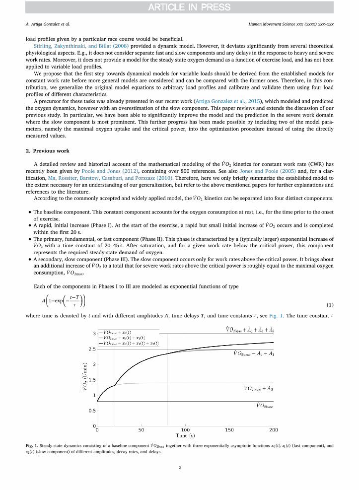
where time is denoted by t and with different amplitudes A, time delays T, and time constants τ , see Fig. 1. The time constant τ

Fig. 1. Steady-state dynamics consisting of a baseline component VO 2base together with three exponentially asymptotic functions x t x t( ), ( )0 1 (fast component), andx t( )2 (slow component) of different amplitudes, decay rates, and delays.

A. Artiga Gonzalez et al. Human Movement Science xxx (xxxx) xxx–xxx

2

determines the time required for the dynamics of the corresponding component to diminish the difference from the asymptoticamplitude A by a factor of − ≈1 1/e 0.632. Thus, after a time of τ3 , about 95% of the amplitude A is reached and the correspondingphase is regarded as effectively having reached its final value. It is important to note that the time delay T is intended to imply thatonly after that time has the oxygen consumption of the corresponding component begun. To complete the model, we thereforeemploy the Heaviside step function (Ma et al., 2010)

= ≥<{H t t

t( ) 1, 00, 0 (2)

setting

⎜ ⎟⎜ ⎟= − ⎛⎝

− ⎛⎝

− − ⎞⎠

⎞⎠

x t A H t T t Tτ

( ) ( ) 1 expk k kk

k (3)

yielding the complete model in one formula as

∑= +=

VO t VO x t ( ) ( ).k

k2 2base0

2

(4)

Here, VO 2base is the baseline component, and the index =k 0,1,2 refers to the components of the three phases, which are para-metrized by their corresponding amplitudes Ak, time delays Tk, and time constants τk. In Phase I there is no delay: =T 00 . This is thestandard form of oxygen dynamics, and is illustrated in Fig. 1.

Phase I typically lasts only a couple of breaths until reaching its target amplitude A0 and during this short period of time at theonset of exercise there is a large variability in the inter breath gas exchange, making it difficult to fit a model to an individualventilatory data series (Whipp, Ward, Lamarra, Davis, &Wasserman, 1982). Therefore, many researchers remove that time periodfrom the data and consider only the first, fast response and the second, slow component (Jones and Poole, 2005, page 26). Thebaseline amplitude would then have to be incremented by the amplitude A0 to compensate for the deletion of Phase I. In this study wealso follow this procedure. Thus, from here on, VO 2base refers to the above mentioned baseline component (renamed VO 2min andmeasured directly) plus an estimated add-on accounting for A0.

In this kinetic model of VO 2 consumption for a constant work rate, the amplitudes Ak must be chosen adaptively. They depend onthe physiological and metabolic condition of the subject and on the applied constant work rate P. Thus, =A A P( )k k . As a firstapproximation, the amplitude of the first, fast component can be taken as a linear function of exercise intensity (power), with slope of9–11 ml/min per Watt of power increase and bounded by VO 2max (Poole and Jones, 2012, page 939).

The second, slow component is more complex. It is the sum of two parts. The first part is an increasing function, which seems tostart having nonzero values from about the gas exchange threshold up to the value of the critical power Pc, where the sum of allcomponents is still less than VO 2max. The exact form of this function has not been determined. For power greater than the criticalpower, the slow component for constant work rate exercise eventually raises the total oxygen consumption up to VO 2max. Thus, for

>P Pc, it can be modeled as an affine linear, decreasing function which is the difference between VO 2max and the sum of theamplitudes of the baseline and the first, fast component.

This model has been validated with CWR and also incremental exercise, where the slow component is not apparent, or at least notfully apparent. In the following section we propose a concrete parametrized model of the total oxygen consumption following thesefindings, summarized in Fig. 5.

Fig. 2. Example of the method of determining the lactate threshold in the lactate curve for Subject 5.

A. Artiga Gonzalez et al. Human Movement Science xxx (xxxx) xxx–xxx

3

3. Methods

3.1. Experimental setup

Six healthy subjects (age 37.8 ± 14.8 yrs, height 180.4 ± 10.1 cm, weight 75.2 ± 7.6 kg) with a cycling background rangingfrom recreational to amateur level gave written informed consent to take part in the study and were thoroughly informed about thetesting procedure. The subjects completed four different cycle ergometer (Cylus2, RBM elektronik-automation GmbH, Leipzig,Germany) tests with continuous breath-by-breath gas exchange and ventilation measurements at the mouth (Ergostik, GerathermRespiratory GmbH, Bad Kissingen, Germany). The first two test protocols were designed to determine a set of physiological para-meters of aerobic capacity that will be employed as upper and lower boundaries for the modeling process. The two remaining testsfeatured varying load profiles in order to comprehensively evaluate the prediction quality of the model.

The following paragraphs describe the four test protocols in detail. See Figs. 3 and 4 for illustrations of the corresponding workrate and road gradient profiles.

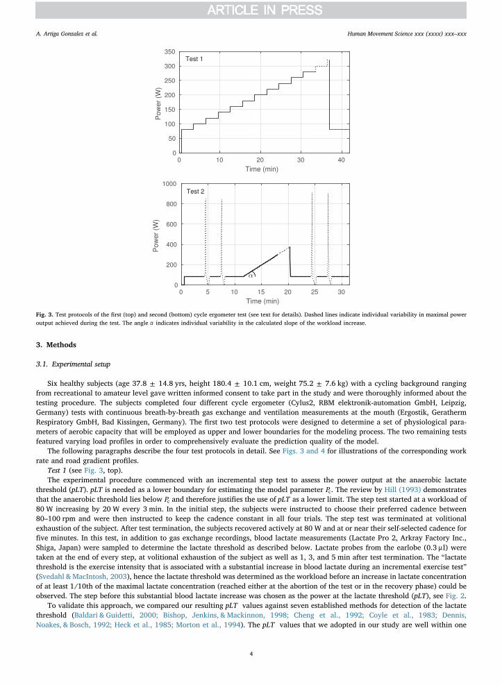
Test 1 (see Fig. 3, top).The experimental procedure commenced with an incremental step test to assess the power output at the anaerobic lactate

threshold (pLT). pLT is needed as a lower boundary for estimating the model parameter Pc. The review by Hill (1993) demonstratesthat the anaerobic threshold lies below Pc and therefore justifies the use of pLT as a lower limit. The step test started at a workload of80 W increasing by 20 W every 3 min. In the initial step, the subjects were instructed to choose their preferred cadence between80–100 rpm and were then instructed to keep the cadence constant in all four trials. The step test was terminated at volitionalexhaustion of the subject. After test termination, the subjects recovered actively at 80 W and at or near their self-selected cadence forfive minutes. In this test, in addition to gas exchange recordings, blood lactate measurements (Lactate Pro 2, Arkray Factory Inc.,Shiga, Japan) were sampled to determine the lactate threshold as described below. Lactate probes from the earlobe (0.3 μl) weretaken at the end of every step, at volitional exhaustion of the subject as well as 1, 3, and 5 min after test termination. The “lactatethreshold is the exercise intensity that is associated with a substantial increase in blood lactate during an incremental exercise test”(Svedahl &MacIntosh, 2003), hence the lactate threshold was determined as the workload before an increase in lactate concentrationof at least 1/10th of the maximal lactate concentration (reached either at the abortion of the test or in the recovery phase) could beobserved. The step before this substantial blood lactate increase was chosen as the power at the lactate threshold (pLT), see Fig. 2.

To validate this approach, we compared our resulting pLT values against seven established methods for detection of the lactatethreshold (Baldari & Guidetti, 2000; Bishop, Jenkins, &Mackinnon, 1998; Cheng et al., 1992; Coyle et al., 1983; Dennis,Noakes, & Bosch, 1992; Heck et al., 1985; Morton et al., 1994). The pLT values that we adopted in our study are well within one

Fig. 3. Test protocols of the first (top) and second (bottom) cycle ergometer test (see text for details). Dashed lines indicate individual variability in maximal poweroutput achieved during the test. The angle α indicates individual variability in the calculated slope of the workload increase.

A. Artiga Gonzalez et al. Human Movement Science xxx (xxxx) xxx–xxx

4

standard deviation of the average of the seven reference values, see Table 1.Test 2 (see Fig. 3, bottom).The second ergometer test consisted of four sprints of 6 s duration each and an incremental ramp test. Two sprints were carried

out before and two after the ramp test to obtain the subjects’ maximal power output and VO 2 profiles in a recovered and a fatiguedstate. Before each set of sprints, the subjects pedaled at 80 W for 5 min at their self-selected cadence. The two sprints of each set wereseparated by 30 s of passive rest and a subsequent 2 min 24 s of active recovery at 80 W. The ergometer load for the sprints wascalculated on the basis the subjects’ body weight multiplied by a factor of 5, expressed in Newton. Ten seconds before each sprint, thesubjects were instructed to increase their cadence gradually in order to obtain their maximal pedaling frequency right at the start ofthe sprint when the load was applied to the flywheel of the ergometer. The subjects were able to time their effort by a countdownvisually presented on a large screen.

In order to obtain approximately the same ramp test time of 10 min for every subject, the end load of the ramp protocol was

Fig. 4. Test protocols of the third (top) and fourth (bottom) cycle ergometer test (see text for details). The dashed line in Test 3 indicates individual variability of timeachieved at 140% of pLT workload.

Fig. 5. Model of the steady state oxygen demand for the baseline, fast, and slow components.

A. Artiga Gonzalez et al. Human Movement Science xxx (xxxx) xxx–xxx

5

estimated individually by the highest exercise intensity reached in the incremental step test multiplied by a factor of 1.3. The startload was set to 80 W, hence the increase per minute was obtained by the following formula: (Individual end load of step test in Watt−start load of 80 W)/ 10 min. The workload was increased every second until the subject terminated the test volitionally.

VT1 was determined visually on the basis of the ramp protocol in Test 2. The method used is described in detail in Beaver,Wasserman, and Whipp (1986). Briefly, plots of VE VCO VE VO/ , /2 2, end-tidal PCO2 (PETCO2), end-tidal PO2 (PETO2) and respiratoryexchange ratio (RER) vs. time were analyzed. The first criterion for VT1 is an increase in the VE VO/ 2 curve after it has declined orstayed constant, without an increase in VE VCO/ 2. The second criterion is a slowly rising or constant PETCO2 curve together with abeginning in the rise of the PETO2 curve after it has had a flat or declining shape. The third criterion is a marked increase in RER aftera horizontal or slowly rising shape. For reasons of simplicity, the lag of theVO 2 increase with respect to the workload of the ramp testhas not been taken into consideration in the determination of VT1 workload.

VO 2max was determined as the highest VO 2 of a 10-value moving average obtained in any of the four tests. In 4 out of 5 subjects,the test with the highest VO 2max was the ramp test. The other subject reached VO 2max in the incremental step test.

VO 2min was determined as the lowest VO 2 value obtained during the 30 s resting phase in any of the four ergometer tests.Table 2 summarizes the parameters from direct measurements and the results.Test 3 (see Fig. 4, top).In the third test, the subjects had to complete a variable step protocol. The steps varied in load and duration and alternated

between low and moderate or severe intensity. The linearly increasing or decreasing intensity between the steps was also varied intime. The intensities were calculated in relation to the pLT. In short, the step protocol looked as follows: 4 min at 80 W, 4 min at 75%pLT, 2 min at 40% pLT, 2 min at 95% pLT, 2 min at 45% pLT, 4 min at 85% pLT, 3 min at 90 W, 2 min at 100% pLT, 5 min at 80 W,2 min at 105% pLT, 2 min at 70 W, 1 min at 60% pLT, and 2 min at 80 W. Fixed workloads for some intervals were used because theergometer was not able to handle workloads that were below 40% of pLT for some subjects. Subsequently, a constant load all-outexercise at 140% pLT followed. This interval lasted from 1.5 to 4.5 min between subjects. The final interval was designed as arecovery ride at 80 W for 5 min.

Test 4 (see Fig. 4, bottom).For the final “synthetic hill climb test” the ergometer was controlled by our simulator software (Dahmen, Byshko, Saupe,

Röder, &Mantler, 2011). The load was defined by a mathematical model (Martin, Milliken, Cobb, McFadden, & Coggan, 1998) tosimulate the resistance on a realistic track. The gradient of that track, depicted in Fig. 4, and the subjects’ body weight were the majordeterminants of the load. While maintaining the same cadence as before, the subjects were able to choose their exercise intensity bygear shifting. (On the steepest section most subjects were not able to maintain the cadence even in the lowest gear.)

Before each session the gas analyzers were calibrated with ambient air and a gas mixture of known composition (15% O2, 5% CO2

and the balance was N). The flow sensor was calibrated by means of a 3-liter syringe. For an adequate recovery, the test sessions wereseparated by at least 48 h. The subjects were instructed to visit the laboratory in a fully recovered state and were asked to refrain fromintense physical activity two days prior to testing. In all test sessions, the subjects received strong verbal encouragement from theinvestigators when they were close to their physical limits. During all the experiments, the subjects were aware of the relevantmechanical variables, such as the power and cadence, displayed on a large screen. The cadence was held constant throughout all testsexcept the sprints in Test 2 and the steep sections (>10% gradient) of Test 4. To obtain a minimal VO 2 (VO 2min) value, subjects stayedseated for 30 s on the ergometer before the start of each test.

Table 1Comparison of the used power at lactate threshold values (pLT, second column) with those from seven established methods for detection of the lactate threshold. Foreach subject the average and the standard deviations with respect to the seven methods are given in the last two columns. All numbers are in Watts and rounded.

pLT Baldari Bishop Cheng Dennis Coyle Heck Morton Average σ(Baldari & Guidetti, 2000) (Bishop et al.,

1998)(Cheng et al.,1992)

(Dennis et al.,1992)

(Coyle et al.,1983)

(Heck et al.,1985)

(Morton et al.,1994)

Subject 1 380 360 382 311 357 369 388 368 362 25Subject 2 240 260 276 225 253 263 283 236 257 21Subject 3 200 180 224 194 219 193 215 214 206 16Subject 4 220 200 226 195 218 203 220 223 212 12Subject 5 260 220 262 225 258 237 267 259 247 19

Average 260 244 274 230 261 253 275 260 257 16

Table 2Parameters extracted from ergometer tests. The averages are over the five study subjects.

Param. Unit Description Average ± σ

VO 2min l/min minimal oxygen uptake 0.354 ± 0.070VT1 W first ventilatory threshold 183 ± 26VO 2max l/min maximal oxygen uptake 4.708 ± 0.873pLT W power at lactate threshold 260 ± 71

A. Artiga Gonzalez et al. Human Movement Science xxx (xxxx) xxx–xxx

6

3.2. The steady-state oxygen demand model

Following the model assumptions from the literature as summarized in Section 2, we propose a steady state oxygen demand givenby a constant baseline component, the first, fast component, and the second, slow component with amplitudes VO A P , ( )2base 1 , andA P( )2 , respectively. The exact form of the slow component for loads below the critical power is not specified in the literature and wepropose an exponential function, parametrized by its amplitude and growth rate. In terms of formulas, the amplitudes are

= −A P s P VO VO( ) min( · , )1 2max 2base (5)

= ⎧⎨⎩

− − ⩽− − >

A PV P P P PVO VO A P P P

( )·exp( ( )/Δ)

( )2Δ c c

2max 2base 1 c (6)

where s is the slope (or gain) for the fast component (about 9–11 ml/min/W), Pc denotes the critical power, VΔ is the maximalamplitude of the slow component for exercise load up to critical power, and Δ is the corresponding decay constant that governs thedecay of the steady-state slow component as the load is decreased from the critical power. Fig. 5 depicts the graph of the sum of allcomponents in this model.

The parameters for this steady state oxygen demand model were determined by least squares fitting to data from one or moreergometer tests (VO P VO s V , , , ,2max c 2base Δ, and Δ, see Table 3). For the fitting procedure, the appropriate search ranges for theparameters are also specified in Table 3. These ranges are based on experimental evidence (VO , Δ2base ) or on constraints of the model.E.g., the upper bound VO P /2max c for the slope s stems from the extreme case where =VO 02base and =VO P VO ( ) 2 c 2max.

We point out that we had previously taken the parameters VO 2max and Pc for our dynamic model of oxygen consumption directlyfrom the ergometer tests (Table 2) (Artiga Gonzalez et al., 2015). However, we found that the model overestimated the slowcomponent because the parameters as measured directly seemed to be too small or too large for the purpose of the model. Therefore,we propose to determine these parameters also by means of parameter fitting instead of direct (and perhaps inappropriate) mea-surements.

3.3. Dynamic model of oxygen consumption

Now let us extend the steady state oxygen demand model so that it becomes dynamic, allowing for a variable load profile P t( ).

The response of the fast and slow components in the case of a constant work rate demand is given by Eq. (1), ⎛⎝

− ⎛⎝

− − ⎞⎠

⎞⎠

A t Tτ

1 exp . Note

that this function is the solution of the linear ordinary differential equation initial value problem

= − =−x τ A x x ( ), (0) 01 (7)

however, delayed by the delay time T or, equivalently, the solution for initial value =x T( ) 0. This suggests the following equationsfor the first and second component, x t x t( ), ( )1 2 ,

= − = =−x τ A P x x T k ( ( ) ), ( ) 0, 1,2k k k k k k1 (8)

defined for times ⩾t Tk (and setting =x t( ) 0k for <t Tk). Here, the power demand is a function of time =P P t( ) and the=A P k( ), 1,2k , are the steady state amplitudes for the fast and slow components given in Eqs. (5) and (6). The totalVO 2 accordingly is

given by

= + +VO t VO x t x t ( ) ( ) ( ).2 2base 1 2 (9)

These differential equations require the four parameters τ τ T, ,1 2 1, and T2 that are listed together with their corresponding ranges inTable 4. These ranges are set in accordance with empirical findings reported in the survey article of Jones and Poole (2005).

We remark that the aboveVO 2 model does not distinguish between on- and off-transient dynamics, i.e., theVO 2 demand and timeconstants are the same regardless of whether the current VO 2 value is below (on-transient case) or above the VO 2 demand (off-transient case). There is, however, some evidence for an asymmetry of dynamics in some of the exercise intensity domains, althoughthis has received little attention in the literature (Poole and Jones, 2012, p. 940). For simplicity, in this paper we stay with thesymmetric model and leave the modeling of asymmetric dynamics for future research.

Table 3Summary of parameters for the model of the steady state oxygen demand.

Param. Unit Description Range

Pc W critical power − −−pLT s VO V VO[ , ( )]1 2max Δ 2base

VO 2base l/min baseline VO 2 − −VO VO V sP[ , ]2min 2max Δ c

VO 2max l/min maximal VO 2 + +VO sP V[ ,measured value])2base c Δs l/min/W exercise economy − −P VO P VO[0.25· , ]c

12max c

12max

VΔ l/min ampl. slow comp. − −VO VO sP[0, ]2max 2base cΔ W range slow comp. −P VT[0, ]c 1

A. Artiga Gonzalez et al. Human Movement Science xxx (xxxx) xxx–xxx

7

3.4. Data preprocessing

In order to estimate the ten parameters of the dynamic model given by Eqs. 5, 6, 8 for a particular subject, the data series of thetime-stamped values of power produced and the resulting breath-by-breath oxygen consumption are required for exercise intensitiesranging from moderate to severe. These time series from ergometer laboratory experiments are typically very noisy, have differentsampling rates for VO 2 and power, and the samples may be irregularly spaced.

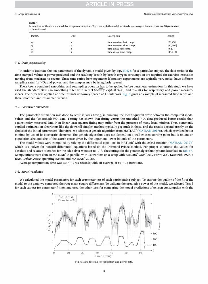
Therefore, a combined smoothing and resampling operator has to be applied before parameter estimation. In this study we haveused the standard Gaussian smoothing filter with kernel −−σ π t σ( 2 ) exp( 0.5 / )1 2 and =σ 20 s for respiratory and power measure-ments. The filter was applied at time instants uniformly spaced at 1 s intervals. Fig. 6 gives an example of measured time series andtheir smoothed and resampled version.

3.5. Parameter estimation

The parameter estimation was done by least squares fitting, minimizing the mean-squared error between the computed modelvalues and the (smoothed) VO 2 data. Testing has shown that fitting versus the smoothed VO 2 data produced better results thanagainst noisy measured data. Non-linear least squares fitting may suffer from the presence of many local minima. Thus, commonlyapplied optimization algorithms like the downhill simplex method typically get stuck in these, and the results depend greatly on thechoice of the initial parameters. Therefore, we adopted a genetic algorithm from MATLAB® (MATLAB, 2017a), which provided betterminima by use of its stochastic elements. The genetic algorithm does not depend on a well chosen starting point but is reliant onpopulation size and size of the search space given by the upper and lower bounds of the parameters.

The model values were computed by solving the differential equations in MATLAB® with the ode45 function (MATLAB, 2017b)which is a solver for nonstiff differential equations based on the Dormand-Prince method. For proper solutions, the values forabsolute and relative tolerance for the ode solver were set to −10 6. The settings for the genetic algorithm (ga) are described in Table 5.Computations were done in MATLAB® in parallel with 16 workers on a setup with two Intel® Xeon® E5-2640 v3 2.60 GHz with 192 GBRAM, Debian Jessie operating system and MATLAB® 2016a.

Average computation time was ±3547 1792 seconds with an average of ±69 15 iterations.

3.6. Model validation

We calculated the model parameters for each ergometer test of each participating subject. To express the quality of the fit of themodel to the data, we computed the root-mean-square differences. To validate the predictive power of the model, we selected Test 3for each subject for parameter fitting, and used the other tests for comparing the model predictions of oxygen consumption with the

Table 4Parameters for the dynamic model of oxygen consumption. Together with the model for steady state oxygen demand there are 10 parametersto be estimated.

Param. Unit Description Range

τ1 s time constant fast comp. [20,45]τ2 s time constant slow comp. [60,300]T1 s time delay fast comp. [0,20]T2 s time delay slow comp. [30,240]

Fig. 6. Data filtering for ventilatory and power data.

A. Artiga Gonzalez et al. Human Movement Science xxx (xxxx) xxx–xxx

8

measured values.

4. Results

The VO 2 model as given by Eqs. 5, 6, 8, 9 was fitted with the least squares method to the data for all four tests and five subjects,resulting in 20 sets of model parameters. The corresponding model errors were calculated by solving the initial value problems in Eq.(8) and summing up the components according to Eq. (9). The resulting model errors are given in Table 7.

Overall, the average VO 2 modeling RMS error was ±0.09 0.03 l/min amounting to an mean absolute percentage error of 3.1%.Fig. 8 illustrates the VO 2 and power data, and the fitting result for Subject 2, whose average RMS error is the median of the errors forsubjects.

In the modeling phase, we found that Test 1 performed best, with the smallest average VO 2 RMS error of 0.06 l/min. Thecorresponding parameter sets for each of the subjects are given in Table 6 and presented in Fig. 7.

In the validation we used the parameters resulting from the model fitting using Test 3 for the prediction of the VO 2 consumptionin the other tests. For the model simulation we used the measured power as input for the differential equations. We present thecorresponding RMS prediction errors in Table 8.

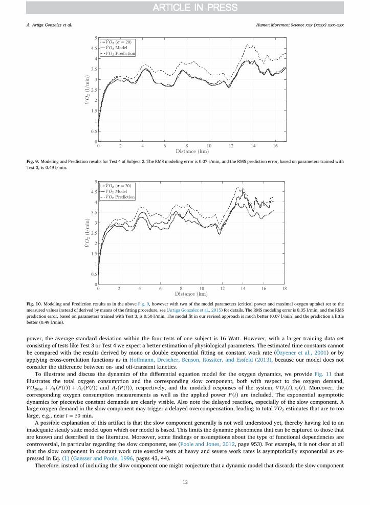
Fig. 9 illustrates the modeling and prediction results for an example. We present the graphs of the VO 2 model fitting, the pre-diction, and the measured VO 2 against time for Test 4, where the subjects were self-pacing themselves. Note that the model pre-diction errors are mostly positive, i.e., the prediction overestimated the actual VO 2 consumption, especially at times of severe

Table 5Settings for the genetic algorithm. Model parameters are normalized be-tween 0 and 1.

PopulationSize 1024

InitialPopulationRange … …[0 0;1 1]MaxStallGenerations 20ConstraintTolerance −10 5

FunctionTolerance −10 5

NonlinearConstraintAlgorithm penalty

Fig. 7. Closeup of the fitted models of steady state oxygen demand for subjects 2 to 5 (compare with Table 6). The discontinuity at the critical power Pc and theexponential parts of the slow component below critical power for subjects 2 and 3 are clearly visible.

Table 6Parameters of the fitted model for the subjects from Test 3.

Parameter VO 2max VO 2base s Pc VΔ Δ T1 τ1 T2 τ2

Unit l/min l/min l/min/W W l/min W min min min min

Subject 1 5.91 1.14 × −10. 2 10 3 383 0.00 – 0:09.3 0:26.4 3:18.4 1:02.8Subject 2 4.63 0.84 × −10. 4 10 3 243 0.63 29 0:04.2 0:25.5 3:04.4 5:00.0Subject 3 3.85 0.56 × −10. 4 10 3 224 0.53 17 0:08.8 0:27.8 3:02.9 5:00.0Subject 4 3.16 0.99 × −9. 1 10 3 217 0.14 28 0:07.7 0:29.7 1:08.6 1:05.6Subject 5 4.87 0.98 × −10. 3 10 3 262 0.00 – 0:10.8 0:32.9 3:58.4 1:06.6

A. Artiga Gonzalez et al. Human Movement Science xxx (xxxx) xxx–xxx

9

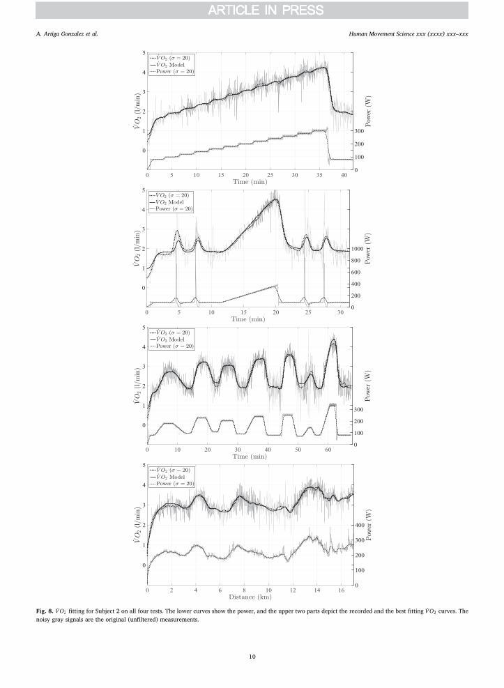
Fig. 8. VO 2 fitting for Subject 2 on all four tests. The lower curves show the power, and the upper two parts depict the recorded and the best fitting VO 2 curves. Thenoisy gray signals are the original (unfiltered) measurements.

A. Artiga Gonzalez et al. Human Movement Science xxx (xxxx) xxx–xxx

10

exercise intensity.

5. Discussion

Overall, the results show that in principle the approach to transferring the dynamic steady-state model from constant work ratesto variable work rates was successful. Parameters could be estimated such that the measured VO 2 data could be approximated with asmall average RMS error of about 0.09 l/min, corresponding to a mean absolute percentage error of 3.1%. For model prediction theaverage error was around 0.30 l/min (MAPE of 8.8%).

An average RMS modeling error of only 0.09 l/min can be regarded as a very satisfactory result. The best one can expect from anoptimal modeling is that the accuracy is in the range of the natural variability of the modeled quantities, and we show that this is thecase here.

We were not able to locate comparable results on the variability of VO 2 kinetics in the literature. Most reproducibility studies arelimited to the investigation of the variability in VO 2max (Dideriksen &Mikkelsen, 2015; Katch, Sady, & Freedson, 1981; Thomas,Cunningham, Rechnitzer, Donner, & Howard, 1987). The few studies investigating the reproducibility of VO 2 kinetics have de-monstrated good measures of reproducibility only for parameters of on- and off-transient kinetics (Cannon, Schenone, & Kolkhorst,2008; de Tarso Müller, Christofoletti, Zagatto, Paulin, & Neder, 2015; Kilding, Challis, Winter, & Fysh, 2005).

Therefore, we carried out an additional small study to investigate the reproducibility of VO 2 kinetics for an incremental exerciseprotocol (unpublished work). In that study, 11 recreationally active subjects performed two identical cycling ramp tests to exhaustionon separate occasions. With the same metabolic unit and analytical methods as used in this study, we gathered VO 2 measurementsover the course of the ramp protocol. We obtained a grand average RMS difference between theVO 2 measurements of the two tests of0.09 l/min and a MAPE of 2.95%, which exactly matches our average RMS modeling error of 0.09 l/min.

We now compare our modeling and prediction results with our previous ones from Artiga Gonzalez et al. (2015). Both, modelingand prediction have been improved, which is illustrated with a typical case given by Test 4 of Subject 2. Fig. 10 shows the results ofArtiga Gonzalez et al. (2015), to be compared with the new results in Fig. 9. In Fig. 10, two of the model parameters (critical powerand maximal oxygen uptake) were set to pLT and VO 2max respectively, instead of being derived by means of the fitting procedure.Also, we increased the range for the time constant and the time delay of the second component and used the same smoothing ( =σ 20)for both, power and VO 2. In summary, with these changes on our revised method the precision of the model fit to the data is muchbetter with 0.09 l/min versus 0.23 l/min and the predictions are a little better with a grand average of 0.30 l/min RMSE versus0.37 l/min in Artiga Gonzalez et al. (2015).

Still, one cannot expect the modeling results to deliver precise estimates of physiological parameters like critical power orVO 2maxor good estimates for the time constants. The parameters we obtain vary according to the training data. For example for critical

Table 8Root-mean-square errors of model predictions for the three tests in the validation set.

Test 1 Test 2 Test 4 Average

RMSE MAPE RMSE MAPE RMSE MAPE RMSE MAPE

l/min % l/min % l/min % l/min %

Subject 1 0.24 5.5 0.50 12.6 0.40 9.3 0.38 9.1Subject 2 0.25 7.3 0.21 7.6 0.49 14.3 0.31 9.7Subject 3 0.14 5.7 0.19 8.3 0.31 8.5 0.21 7.5Subject 4 0.32 9.4 0.19 7.3 0.18 5.2 0.23 7.3Subject 5 0.30 9.0 0.19 5.5 0.67 17.0 0.38 10.5

Average 0.25 7.4 0.25 8.3 0.41 10.8 0.30 8.8

Table 7Errors of model fit. Parameters have been fitted for each case separately. The approximation quality is expressed by root-mean-square error (RMSE) and mean absolutepercentage error (MAPE).

Test 1 Test 2 Test 3 Test 4 Average

RMSE MAPE RMSE MAPE RMSE MAPE RMSE MAPE RMSE MAPE

l/min % l/min % l/min % l/min % l/min %

Subject 1 0.08 2.3 0.25 7.3 0.11 3.1 0.08 1.8 0.13 3.6Subject 2 0.05 2.0 0.14 5.2 0.10 3.5 0.07 2.3 0.09 3.2Subject 3 0.04 1.8 0.08 3.2 0.05 2.1 0.07 2.3 0.06 2.3Subject 4 0.07 2.7 0.10 4.2 0.17 4.9 0.08 2.4 0.10 3.6Subject 5 0.05 1.7 0.13 4.1 0.09 3.3 0.09 1.8 0.09 2.7

Average 0.06 2.1 0.14 4.8 0.10 3.4 0.08 2.1 0.09 3.1

A. Artiga Gonzalez et al. Human Movement Science xxx (xxxx) xxx–xxx

11

power, the average standard deviation within the four tests of one subject is 16 Watt. However, with a larger training data setconsisting of tests like Test 3 or Test 4 we expect a better estimation of physiological parameters. The estimated time constants cannotbe compared with the results derived by mono or double exponential fitting on constant work rate (Özyener et al., 2001) or byapplying cross-correlation functions as in Hoffmann, Drescher, Benson, Rossiter, and Essfeld (2013), because our model does notconsider the difference between on- and off-transient kinetics.

To illustrate and discuss the dynamics of the differential equation model for the oxygen dynamics, we provide Fig. 11 thatillustrates the total oxygen consumption and the corresponding slow component, both with respect to the oxygen demand,

+ +VO A P t A P t ( ( )) ( ( ))2base 1 2 and A P t( ( ))2 , respectively, and the modeled responses of the system, VO t x t ( ), ( )2 2 . Moreover, thecorresponding oxygen consumption measurements as well as the applied power P t( ) are included. The exponential asymptoticdynamics for piecewise constant demands are clearly visible. Also note the delayed reaction, especially of the slow component. Alarge oxygen demand in the slow component may trigger a delayed overcompensation, leading to total VO 2 estimates that are to toolarge, e.g., near =t 50 min.

A possible explanation of this artifact is that the slow component generally is not well understood yet, thereby having led to aninadequate steady state model upon which our model is based. This limits the dynamic phenomena that can be captured to those thatare known and described in the literature. Moreover, some findings or assumptions about the type of functional dependencies arecontroversial, in particular regarding the slow component, see (Poole and Jones, 2012, page 953). For example, it is not clear at allthat the slow component in constant work rate exercise tests at heavy and severe work rates is asymptotically exponential as ex-pressed in Eq. (1) (Gaesser and Poole, 1996, pages 43, 44).

Therefore, instead of including the slow component one might conjecture that a dynamic model that discards the slow component

Fig. 9. Modeling and Prediction results for Test 4 of Subject 2. The RMS modeling error is 0.07 l/min, and the RMS prediction error, based on parameters trained withTest 3, is 0.49 l/min.

Fig. 10. Modeling and Prediction results as in the above Fig. 9, however with two of the model parameters (critical power and maximal oxygen uptake) set to themeasured values instead of derived by means of the fitting procedure, see (Artiga Gonzalez et al., 2015) for details. The RMS modeling error is 0.35 l/min, and the RMSprediction error, based on parameters trained with Test 3, is 0.50 l/min. The model fit in our revised approach is much better (0.07 l/min) and the prediction a littlebetter (0.49 l/min).

A. Artiga Gonzalez et al. Human Movement Science xxx (xxxx) xxx–xxx

12

would yield better prediction results. In Artiga Gonzalez et al. (2015) we checked this in a quick test by removing the slow componentin the parameter fitting procedure. The results for prediction of Test 4 indicated a good improvement. However, for the othervalidation tests the predictions using the slow component were better. Still, this indicates that there is a good opportunity forimprovements of the mathematical model beyond the direct transfer from constant to variable work rates.

6. Conclusions and future research

We contributed to the generalization of the commonly accepted model of the dynamics of oxygen uptake during exercise atconstant work rates to variable load protocols by means of differential equations. We showed how the parameters in the model can beestimated and that the mathematical dynamical model can be used to predict the oxygen consumption for other load profiles. Wefound for five subjects and four very different test protocols (of up to about one hour in length) that on average the modeling RMSerror of VO 2 was ±0.09 0.03 l/min and the prediction RMS error in three tests was ±0.30 0.09 l/min.

An alternative approach to modeling would be to allow for different, more appropriate degrees of freedom in the mathematicalmodel, again fitting the model type and parameters to empirical data, and calculating the model and prediction errors. For example,we could assume as above two additive model components (besides a constant baseline oxygen consumption) with different delaytimes and decay rates, however, with corresponding steady state oxygen demands that are restricted only by requiring (piecewise)monotonicity and that can be parametrized by a set of 10 parameters, the same number as in this paper. Moreover, as mentionedabove, there is evidence for an asymmetry between on- and off-transient dynamics, i.e., the VO 2 demand and time constants shouldbe defined differently depending on whether the current VO 2 value is below (on-transient case) or above the VO 2 demand (off-transient case).

With such an approach, we expect a better data fitting. It remains an open question whether also the predictive power would bebetter than for our current model and whether the results could be interpreted in harmony with the current understanding of sportphysiology and sport medicine.

Acknowledgment

This work has been supported by a research grant of the Deutsche Forschungsgemeinschaft (DFG) for the project “Powerbike –Model-based optimization for road cycling.”

We thank the anonymous reviewers for their very helpful comments and suggestions.

References

Artiga Gonzalez, A., Bertschinger, R., Brosda, F., Dahmen, T., Thumm, P.,, & Saupe, D. (2015). Modeling oxygen dynamics under variable work rate. icSPORTS 2015:3rd International congress on sport sciences research and technology support (pp. 198–207). .

Baldari, C., & Guidetti, L. (2000). A simple method for individual anaerobic threshold as predictor of max lactate steady state.Medicine and science in sports and exercise,32(10), 1798–1802.

Beaver, W. L., Wasserman, K., & Whipp, B. J. (1986). A new method for detecting anaerobic threshold by gas exchange. Journal of Applied Physiology, 60(6),2020–2027.

Bishop, D., Jenkins, D. G., & Mackinnon, L. T. (1998). The relationship between plasma lactate parameters, wpeak and 1-h cycling performance in women. Medicineand Science in Sports and Exercise, 30(8), 1270–1275.

Cannon, D. T., Schenone, A., & Kolkhorst, F. W. (2008). On the reproducibility of oxygen uptake kinetics during heavy exercise. The FASEB Journal, 22, 1176–1178(1MeetingAbstracts).

Cheng, B., Kuipers, H., Snyder, A., Keizer, H., Jeukendrup, A., & Hesselink, M. (1992). A new approach for the determination of ventilatory and lactate thresholds.International Journal of Sports Medicine, 13(07), 518–522.

Coyle, E. F., Martin, W. H., Ehsani, A. A., Hagberg, J. M., Bloomfield, S. A., Sinacore, D. R., & Holloszy, J. O. (1983). Blood lactate threshold in some well-trained

Fig. 11. Steady-state demand and dynamic model for Subject 2 on Test 3. See text for details.

A. Artiga Gonzalez et al. Human Movement Science xxx (xxxx) xxx–xxx

13

ischemic heart disease patients. Journal of Applied Physiology, 54(1), 18–23.Dahmen, T. (2012). Optimization of pacing strategies for cycling time trials using a smooth 6-parameter endurance model. Proceedings pre-olympic congress on sports

science and computer science in sport (IACSS), Liverpool, England, UK, July 24–25.Dahmen, T., Byshko, R., Saupe, D., Röder, M., & Mantler, S. (2011). Validation of a model and a simulator for road cycling on real tracks. Sports Engineering, 14(2–4),

95–110.de Tarso Müller, P., Christofoletti, G., Zagatto, A. M., Paulin, F. V., & Neder, J. A. (2015). Reliability of peak O 2 uptake and O 2 uptake kinetics in step exercise tests in

healthy subjects. Respiratory Physiology & Neurobiology, 207, 7–13.Dennis, S. C., Noakes, T. D., & Bosch, A. N. (1992). Ventilation and blood lactate increase exponentially during incremental exercise. Journal of Sports Sciences, 10(5),

437–449.Dideriksen, K., & Mikkelsen, U. R. (2015). Reproducibility of incremental maximal cycle ergometer tests in healthy recreationally active subjects. Clinical Physiology

and Functional Imaging.Gaesser, G. A., & Poole, D. C. (1996). The slow component of oxygen uptake kinetics in humans. Exercise and Sport Sciences Reviews, 24(1), 35–70.Heck, H., Mader, A., Hess, G., Mücke, S., Müller, R., & Hollmann, W. (1985). Justification of the 4-mmol/l lactate threshold. International Journal of Sports Medicine,

6(03), 117–130.Hill, D. W. (1993). The critical power concept. Sports Medicine, 16(4), 237–254.Hoffmann, U., Drescher, U., Benson, A., Rossiter, H., & Essfeld, D. (2013). Skeletal muscle V O2 kinetics from cardio-pulmonary measurements: assessing distortions

through O2 transport by means of stochastic work-rate signals and circulatory modelling. European Journal of Applied Physiology, 113(7), 1745–1754.Jones, A. M., & Poole, D. C. (2005). Introduction to oxygen uptake kinetics and historical development of the discipline. In A. M. Jones, & D. C. Poole (Eds.). Oxygen

uptake kinetics in sport, exercise and medicine (pp. 3–35). London: Routledge.Katch, V. L., Sady, S. S., & Freedson, P. (1981). Biological variability in maximum aerobic power. Medicine and Science in Sports and Exercise, 14(1), 21–25.Kilding, A., Challis, N., Winter, E., & Fysh, M. (2005). Characterisation, asymmetry and reproducibility of on-and off-transient pulmonary oxygen uptake kinetics in

endurance-trained runners. European Journal of Applied Physiology, 93(5–6), 588–597.Ma, S., Rossiter, H. B., Barstow, T. J., Casaburi, R., & Porszasz, J. (2010). Clarifying the equation for modeling of VO 2 kinetics above the lactate threshold. Journal of

Applied Physiology, 109(4), 1283–1284.Martin, J. C., Milliken, D. L., Cobb, J. E., McFadden, K. L., & Coggan, A. R. (1998). Validation of a mathematical model for road cycling power. Journal of Applied

Biomechanics, 14, 276–291.MATLAB® (2017a). Global Optimization Toolbox™: User’s Guide (R2017a). MathWorks®.MATLAB® (2017b). MATLAB®: Mathematics (R2017a). MathWorks®.Morton, R., Fukuba, Y., Banister, E., Walsh, M., Kenny, C. T., & Cameron, B. (1994). Statistical evidence consistent with two lactate turnpoints during ramp exercise.

European Journal of Applied Physiology and Occupational Physiology, 69(5), 445–449.Özyener, F., Rossiter, H. B., Ward, S. A., & Whipp, B. J. (2001). Influence of exercise intensity on the on-and off-transient kinetics of pulmonary oxygen uptake in

humans. The Journal of Physiology, 533(3), 891–902.Poole, D. C., & Jones, A. M. (2012). Oxygen uptake kinetics. Comprehensive. Physiology, 2, 933–996.Stirling, J., Zakynthinaki, M., & Billat, V. (2008). Modeling and analysis of the effect of training on VO 2 kinetics and anaerobic capacity. Bulletin of Mathematical

Biology, 70(5), 1348–1370.Svedahl, K., & MacIntosh, B. R. (2003). Anaerobic threshold: the concept and methods of measurement. Canadian Journal of Applied Physiology, 28(2), 299–323.Thomas, S., Cunningham, D., Rechnitzer, P., Donner, A., & Howard, J. (1987). Protocols and reliability of maximal oxygen-uptake in the elderly. Canadian Journal of

Sport Sciences, 12(3), 144–151.Whipp, B. J., & Rossiter, H. B. (2005). The kinetics of oxygen uptake: Physiological inference from the parameters. In A. M. Jones, & D. C. Poole (Eds.). Oxygen uptake

kinetics in sport, exercise and medicine (pp. 62–94). London: Routledge.Whipp, B. J., Ward, S. A., Lamarra, N., Davis, J. A., & Wasserman, K. (1982). Parameters of ventilatory and gas exchange dynamics during exercise. Journal of Applied

Physiology, 52(6), 1506–1513.

A. Artiga Gonzalez et al. Human Movement Science xxx (xxxx) xxx–xxx

14