HSC Chemistry 7.0 User's Guide Sim Experimental.pdf · HSC Chemistry ® 7.0 47 - 1 Pertti Lamberg...

HSC Chemistry® 7.0 47 - 1

Pertti Lamberg October 12, 2009 09006-ORC-J

HSC Chemistry® 7.0 User's Guide

Sim Flowsheet Module – Experimental Mode

Pertti Lamberg

Outotec Research Oy Information Service P.O. Box 69 FIN - 28101 PORI, FINLAND

Fax: +358 - 20 - 529 - 3203

Tel: +358 - 20 - 529 - 211

E-mail: [email protected] www.Outotec.com/hsc



47. EXPERIMENTAL MODE

47.1. General

HSC Sim 7.0 has a new Experimental mode that has been designed to process data from

laboratory/pilot testwork or from plant surveys. Besides organizing the original

measurements it is possible to Mass Balance and Reconcile the experimental data.

The features of the HSC Sim 7.0 are:

• You can use the very same drawing and visualization tools as in the simulation

modes (see chapters 42-43).

• You can bring in your chemical assays and other measurements from the process and

visualize using Sankey diagrams and flowsheet tables.

• For Mass Balancing and Data Reconciliation there is no need to draw a new

flowsheet; HSC Sim 7.0 will create the mass balancing nodes according to your data.

You can easily ignore some streams or analyses.

With HSC Sim 7.0 you can solve the following types of mass balance problems:

1. Reconcile measured or estimated component flowrates (1D components).

2. Mass balance and reconcile chemical analyses (1D assays)

3. Mass balance minerals in a minerals processing circuit (1D Minerals)

4. Mass balance size distribution and water balance (1.5D)

5. Mass balance assays and components in 2 or 3 phase systems where bulk

composition is not analyzed (2D Components)

6. Mass balance minerals or chemical assays size-by-size (2D Assays)

7. Mass balance particles, MLA assays (3D)

For more information about mass balancing, please see the “48 Sim Mass Balancing”

manual.

47.2. Experimental Mode

The Experimental mode has been designed to process data that is produced in laboratory

tests or sampled in process surveys. The steps of using Experimental Mode are:

1. Select File – New Process and select Experimental Mode (Figures 1-2)

• Optionally you can change the mode later to Experimental or you can toggle

between one of the simulation modes (Particle, Hydro, Pyro) and the

Experimental Mode (Figure 3)

2. Draw the flowsheet (for more details on drawing see the Sim manual: “40 Sim Flowsheet”

• Select units tab (Figure 4)

• Drag and drop on the drawing area

• Rename the unit using the “Process” tab and NameID field (Figure 5)

• Draw the Streams and rename them (Figure 6)

• Check the stream connections (Figure 7)

• Check for errors (Figure 8)

• Save the flowsheet (create a new folder) (Figure 9)



3. Select from the menu Experimental – Analyses

4. Create the experimental tables, select Create – Experimental Tables (All) from the menu.

5. Save the Experimental data (File – Save).

Figure 1. Selecting a new process, File New…

Figure 2. Select Experimental.

Figure 3. Switching between the simulation modes (Particle / Reactions / Distribution) and the

Experimental mode.



Figure 4. Select units from the ”Units” tab.

Figure 5. Name the unit, use the ”Process” tab and NameID field



Figure 6. Drawing the streams.

Figure 7. Checking for stream connections, the color indicates the stream type: blue = input

stream, red = output stream, black = intermediate stream, light blue = stream without source and

destination.



Figure 8. Checking for errors.

Figure 9. Saving the file, Save Process As…

Figure 10. Create – Experimental Tables (All).



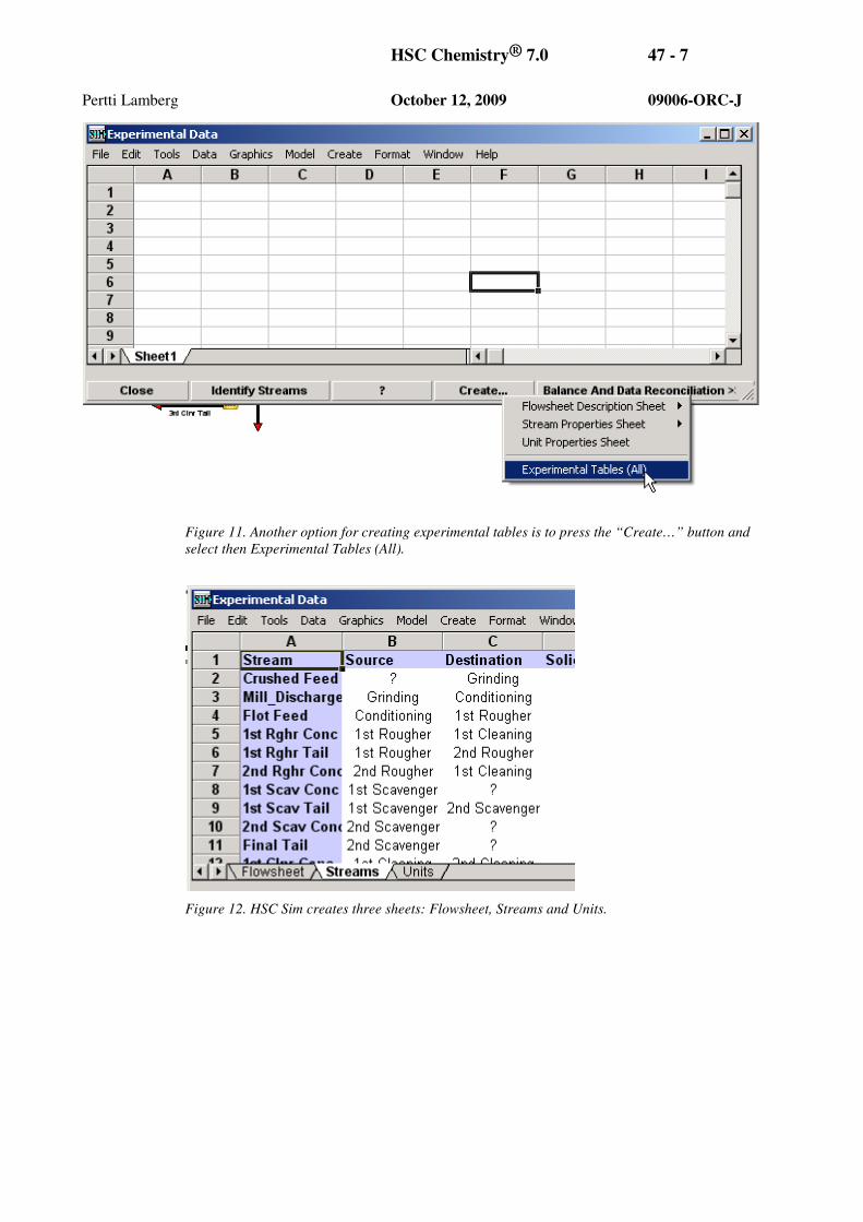
Figure 11. Another option for creating experimental tables is to press the “Create…” button and

select then Experimental Tables (All).

Figure 12. HSC Sim creates three sheets: Flowsheet, Streams and Units.



47.3. Bringing in the Experimental Data

You can bring in your experimental data to the HSC Sim for data visualization and mass

balancing. The easiest way is to bring the data using the clipboard, another way is to bring

the data manually.

47.3.1. Using Clipboard To bring the data from e.g. Excel to HSC Sim the easiest way is to use the clipboard. To do

that:

• Arrange your data in Excel row-wise, each stream is one row

• Use only one header row

• The column including the stream names should be named “Streams”

• The columns including assays should be named using a syntax: element-separator-

method-separator-unit, e.g. Cu XRF % (here the separator is space), SiO2_TOT_%,

and Au FA g/t. You can leave the method out if you like, e.g. Cu %, As %, Ag g/t,

Au ppm.

• Copy the data into the clipboard, the Stream cell should be the top-left cell selected

(Figure 13).

• Select the Streams –sheet (page) and select from the menu Edit – Paste Special

Assays (Figure 14)

• You can freeze the panes to see the stream name column and the header column to

be always visible as you scroll the data sheet (Figure 15).

• Your data is now arranged in HSC Sim. (Figure 16)

• If HSC has not identified a certain stream, it is pasted last on the list and both the

Source and Destination fields are empty (Figure 17-18).

• To re-identify the stream type the correct name and press the “Identify Streams”

button (Figure 18).

Figure 13. Data in Excel, copying into the clipboard .



Figure 14. Pasting the assays

Figure 15. Freezing panes.



Figure 16. Data in HSC Sim.

Figure 17. Unidentified stream: ROM.



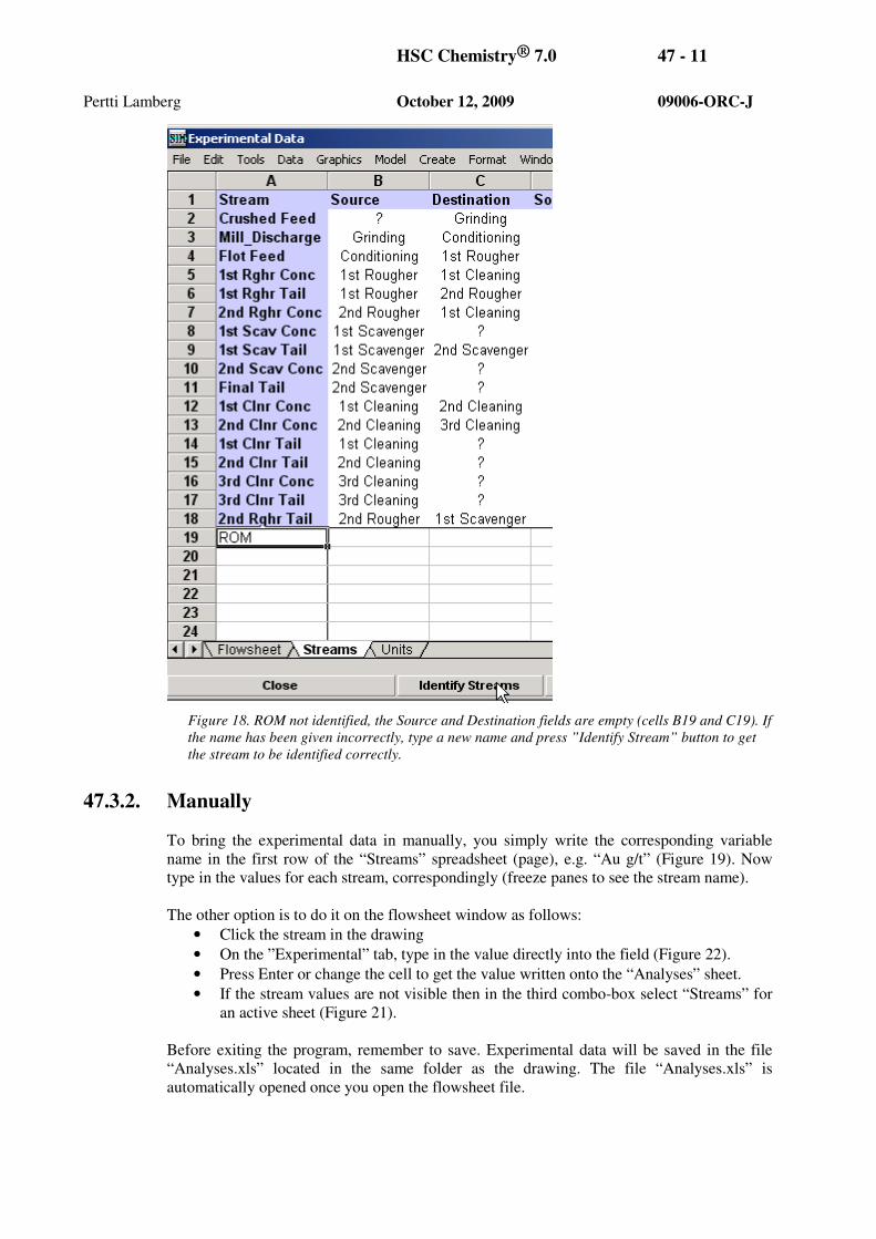
Figure 18. ROM not identified, the Source and Destination fields are empty (cells B19 and C19). If

the name has been given incorrectly, type a new name and press ”Identify Stream” button to get

the stream to be identified correctly.

47.3.2. Manually

To bring the experimental data in manually, you simply write the corresponding variable

name in the first row of the “Streams” spreadsheet (page), e.g. “Au g/t” (Figure 19). Now

type in the values for each stream, correspondingly (freeze panes to see the stream name).

The other option is to do it on the flowsheet window as follows:

• Click the stream in the drawing

• On the ”Experimental” tab, type in the value directly into the field (Figure 22).

• Press Enter or change the cell to get the value written onto the “Analyses” sheet.

• If the stream values are not visible then in the third combo-box select “Streams” for

an active sheet (Figure 21).

Before exiting the program, remember to save. Experimental data will be saved in the file

“Analyses.xls” located in the same folder as the drawing. The file “Analyses.xls” is

automatically opened once you open the flowsheet file.



Figure 19. Adding a new variable, i.e. measured property, of the streams, “Au g/t.”

Figure 20. Typing in the values for ”Au g/t.”

Figure 21. Activate the ”Streams” sheet in the ”Experimental” tab.



Figure 22. Click the stream in the drawing and on the ”Experimental” tab. type in the value

directly into the field (for example Au g/t).

47.4. Visualizing the Analyses

47.4.1. Stream Value Labels and Sankey Diagram

Once you have successfully brought your experimental data into “Analyses” you can

visualize the analyzed values on the flowsheet. To do that:

• In the bottom right-hand corner press Visualize and select “Create Stream Value

Labels” (Figure 23)

• HSC Sim will create “Stream Value Labels” and a “Stream Header Label”

• You can change the styles of the objects (select them and use the “Drawing” tab to

change font size and color.

• To visualize a variable on the flowsheet with a Sankey diagram: 1) select the

variable in the “Analyses” window. Then, select the whole column (Figure 25)

• Click the stream and in the “Experimental” tab select the variable and use the right

mouse to select “Visualize” (Figure 26).



Figure 23. Selecting streams.

Figure 24. HSC Sim has created the “Stream Value Labels” (shows as [value]) and “Stream

Header Label” (shown as [header]).



Figure 25. To visualize, select the whole column by clicking the column header.



Figure 26. Visualizing a variable with a Sankey diagram from the “Experimental” tab.

47.4.2. Stream Tables

You can also visualize using Stream Tables.

• In the “Experimental” tab, press the “Visualize” button and select “Create Stream

Tables” (Figure 27)

• In the “Experimental” tab, activate the variable you want to show in the table.

• Press the right button and select “Show in Table” (Figure 28)

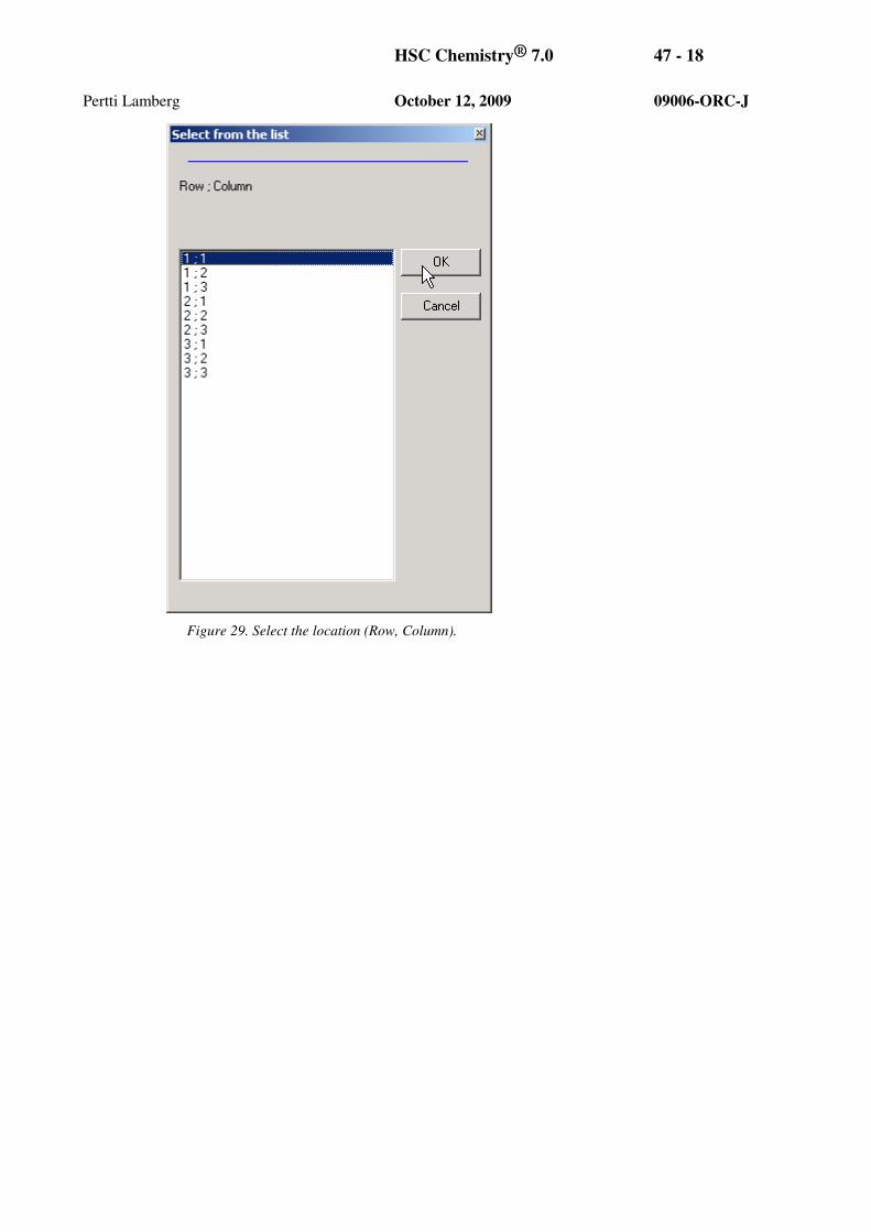
• Select the coordinate (Row:Column) (Figure 29)

• Continue to assign other variables (Figure 30)

• Formulate the tables by double-clicking any of the table, changing the settings (font

type, size, color; cell pattern; row height) and then use Format to apply style, size

and dimensions to all tables.

• Add other elements like tables, texts, and drawings onto the flowsheet (Figure 31).

• Use Print, or Copy Paste to report out.



Figure 27. Creating Stream Tables.

Figure 28. Select the variable and with the right mouse select “Show in Table..”



Figure 29. Select the location (Row, Column).



Figure 30. Tables created and Cu % and S % assigned.



Figure 31. Graphical objects added to the flowsheet.

47.5. Example

See the example in folder HSC7\Flowsheet_Experimental\Example - Laboratory Flotation

Test. The LabTestData.xls file gives the assays. If you want to rehearse how to bring the

experimental data into HSC Sim, copy the flowsheet file “Laboratory Flotation Test.fls” into

another (empty) folder and work as described in chapter 47.3.

Please check the HSC Forum (www.hsc-chemistry.com, Forum; or directly http://www.hsc-

chemistry.com/forum_v3/) for updates and new examples.

HSC Chemistry 7.0 User's Guide Sim Experimental.pdf · HSC Chemistry ® 7.0 47 - 1 Pertti Lamberg...

Documents

Transcript of HSC Chemistry 7.0 User's Guide Sim Experimental.pdf · HSC Chemistry ® 7.0 47 - 1 Pertti Lamberg...