How Does ENSO Impact the Solar Radiation Forecast inSouth America? The Self-affinity Analysis Approach

T.B. Muraria,∗, A.S. Nascimento Filhoa, M.A. Moreta,b, S. Pitomboa, A.A.B.Santosa

aCentro Universitário Senai Cimatec, Salvador, BA, BrazilbUniversidade do Estado da Bahia, Salvador, BA, Brazil

Abstract

The major challenge we face today in the energy sector is to meet the growing

demand for electricity with less impact on the environment. South America is

an important player in the renewable energy resource. Brazil accelerated the

growth of photovoltaic installed capacity in 2018. From April of 2017 to April

of 2018, the capacity increased 1351.5%. It is expected to reach the value of

2.4 GW until the end of the year. The new Chilean regulation request that 20%

of the total electricity production in 2025 must come from renewable energy

sources. The aim of this paper is to establish time series behavior changes

between El Niño Southern Oscillation and the solar radiation resource in South

America. The results can be used to validate forecasts of energy production for

new solar plants. The method used to verify the behavior of the time series

was the Detrended Fluctuation Analysis. Solar radiation data were collected

in twenty-five cities distributed inside the Brazilian solar belt, plus six cities in

Chile, covering the continent from east to west, in a region with high potential of

solar photovoltaic generation. The results shows the impact of El Niño Southern

Oscillation on the climatic behavior of the evaluated data. It is a factor that

∗Corresponding authorEmail addresses: mura.learning@gmail.com (T.B. Murari ),

aloisio.nascimento@gmail.com (A.S. Nascimento Filho), mamoret@gmail.com (M.A. Moret),sergio.pitombo@fieb.org.br (S. Pitombo), alex.santos@fieb.org.br (A.A.B. Santos)

Preprint submitted to Elsevier November 9, 2021

arX

iv:2

007.

1563

7v1

[ph

ysic

s.ao

-ph]

23

Jul 2

020

may lead to the wrong forecast of the long term potential solar power generation

for the region.

Keywords: Solar Radiation; DFA; Photovoltaic Energy Plant; ENSO

1. Introduction

Renewable energy sources can play an important role in solving the dilemma

of increasing energy production capacity by minimizing interference in the en-

vironment [1]. Some studies have been investigating the potential contribution

of renewable energy supplies to the global grid. It indicates that, in the second

half of this century, their contribution might range from 20% to more than 50%,

once we established the correct government policies [2].

Regarding renewable energy investments, Brazil and Chile stand out in South

America continent. Both are the first and second destination countries for for-

eign investment, in clean energy asset finance, in the region, attracting the most

investment from overseas financiers from 2010 up to 2016. Brazil received US$

12.78 billions and Chile, US$ 6.92 billions. For reference, in the same period,

Latin America received a total of US$ 36.1 billions in clean energy investment

from overseas funders [3].

The installed capacity of power generation in Brazil reached 150.4 GW in

2016, an increase of 9.5 GW in relation to 2015. Among the sources that stand

out most are hydropower, with 64.5%, and biomass, which held 9.3%. Con-

sidering this import source, the total power supply reached 156.3 GW in 2016.

Thus, 80.6% of Brazil’s total installed energy capacity is renewable, while, in

the world, the indicator is only 33%, close to 6450 GW [4].

2

According to the monthly monitoring bulletin of the Brazilian Electric Sys-

tem, the solar photovoltaic source in Brazil grown rapidly in recent years. Brazil

reach the end of 2018 with 2400 MW. Further, the 10-year Energy Expansion

Plan (PDE 2024) estimates that the installed capacity of solar generation in

Brazil will reach 8300 MW by 2024. For instance, the Brazilian installed solar

energy capacity increased 1351.5% from April of 2017 to 2018 [5].

In Brazil, a Certified Energy Production Estimative (CEPE) for the future

solar plant must be submitted to the government, by the interested company

who wants to participate in auctions to generate this photovoltaic energy. This

estimation is calculated based on, at least, twelve consecutive months of mea-

surements within a radius of up to 10km from the project. In addition to

horizontal solar radiation, data on temperature, relative air humidity and wind

speed need to be collected. The rate of data loss must be less than 10% of the

total and the absence of continuous measurements can not exceed fifteen days

[4]. According to [6], solar radiation and temperature are the two main factors

that influence energy production by photovoltaic modules.

The local measured data is compared with the same period data obtained

from satellite models to obtain the Typical Meteorological Year, that is used in

the calculation of CEPE. Moreover, these certified data will be correlated with

a dataset collected from the closest weather station, for 10 years or more [4].

Brazil has great potential for photovoltaic power generation. The North-

eastern region has the highest potential of the country, with a mean value of

the solar Global Horizontal Irradiance (GHI) of 5.9 kWh/m2. This high rate

in the Northeast is explained by the low cloudiness condition [7]. The Figure

3

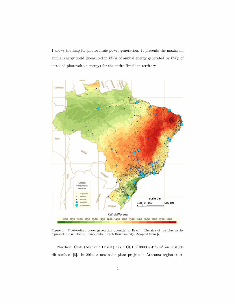
1 shows the map for photovoltaic power generation. It presents the maximum

annual energy yield (measured in kWh of annual energy generated by kWp of

installed photovoltaic energy) for the entire Brazilian territory.

Figure 1: Photovoltaic power generation potential in Brazil. The size of the blue circlesrepresent the number of inhabitants in each Brazilian city. Adapted from [7]

Northern Chile (Atacama Desert) has a GUI of 3300 kWh/m2 on latitude

tilt surfaces [8]. In 2014, a new solar plant project in Atacama region start,

4

and it will be the largest solar project in Latin America, to be used particularly

for mining companies with operations in the region [9]. The country can meet

the 20% target of its capacity from renewable sources, before the 2025 deadline

[10], even in the absence of government subsidies [9]. Beside that, Chile was the

first country in Latin America to create a carbon tax. The Congress passed the

called green tax in September of 2014 [9].

South America is impacted by the El Niño Southern Oscillation (ENSO).

Both El Niño and La Niña climate phenomenas are known as ENSO and they

are the opposite phases of a natural climate pattern throughout the tropical

Pacific Ocean ecosystem, which oscillates every 3 to 7 years [11, 12]. These

events lead to significant differences in the average temperature of the oceans,

winds, surface pressure and precipitation in parts of the Tropical Pacific Ocean

[11].

Brazil has an energy matrix with a renewable-thermal configuration, but, es-

sentially, depends on a large hydropower plants, which can be an issue in times

of severe drought. For instance, Brazil had some severe drought on Amazon

region in the years of 2005 [13], 2010 [14] and 2016 [15]. The same drought

condition was experienced by Northeastern region in 2005, 2007, 2010, 2012

and 2016 [15, 16]. It is one factor that may justify the current growth of non-

hydropower plants in the country [5].

El Niño is associated with above average rainfall in central Chile during win-

ter and late spring. The La Niña is related to the below average rainfall in the

same period and region. El Niño is dry and La Niña wet in southern-central

Chile during the summer [17]. There is also a study about the techno-economical

5

impact in the wind resource of Chile [18].

Table 1 shows the occurrences of El Niño and La Niña in the world and their

intensities based on the Oceanic Niño Index values from 1950 to 2018. Events

were classified as weak, moderate, strong or very strong [19, 20].

Table 1: El Niño and La Niña occurrences [11]

El Niño La NiñaWeak Moderate Strong Very Strong Weak Moderate Strong1952-53 1951-52 1957-58 1982-83 1954-55 1955-56 1973-741953-54 1963-64 1965-66 1997-98 1964-65 1970-71 1975-761958-59 1968-69 1972-73 2015-16 1971-72 1995-96 1988-891969-70 1986-87 1987-88 1974-75 2011-12 1998-991976-77 1994-95 1991-92 1983-84 1999-001977-78 2002-03 1984-85 2007-081979-80 2009-10 2000-01 2010-112004-05 2005-062006-07 2008-092014-15 2016-17

South America is a drought hot spot in some future weather projections

because of its potential to drastically react to excessive warming and drying

[16, 21], and El Niño events are important predictors for severe droughts over

the Brazilian Amazon and Northeast [22, 23]. The greatest analyzed drought,

between 1982 and 2017, is the known 2016 drought, during the El Niño, an

unprecedented dry period [15].

Significant local studies on the effects of the ENSO in various parts of

the globe have been important in establishing the prediction of solar energy

[24, 25, 26]. [27] provides an overview study of the decrease of solar radiation

for four climatic zones of northeastern Brazil, which can be attributed to the

global dimming effect influenced by ENSO. On the other hand, the variability

6

of the solar irradiation in the Atacama desert is influenced by the ENSO. These

phenomena will result in years with significantly different solar irradiation than

TMY [28]. The time series solar radiation exhibit characteristics associated

with natural climatic phenomena with example ENSO, thus revealing that the

Descending Solar Radiation can be considered as an indirect indicator for these

[29].

It brings out the following question: Does ENSO uniformly impact the solar

radiation and, consequently, the forecast of solar power production in South

America? The aim of this paper is to establish time series behavior changes

between ENSO and the solar radiation resource spatially. These relationships

may be used to guide forecasts for new solar energy plants. Therefore, the scope

of this work is limited to the evaluation of the solar radiation variable.

2. Materials and methods

2.1. Dataset Acquisition

All measurements represents the accumulated solar radiation per 3 hours

(MJ/m2) and it were provided by the Brazilian Center for Weather Forecast-

ing and Climate Studies (CPTEC) of the National Institute for Space Research

(INPE) [30] and the National Agro-climatic Network (Agromet) of Chile [31].

This data was automated collected from weather stations that are widely dis-

tributed in several regions of Brazil, within the solar belt [32], and Chile. The

chosen region has a huge potential for solar power generation. It was evaluated

datasets from thirty one cities that reach a maximum threshold of 10% of lost

data inside this region (Figure 2 and Table 2). The lost data were removed from

the city dataset. An example of these time series can be seen on 3, that rep-

7

resent the collected data from Piatã during the El Niño, between 2015 and 2016.

This threshold was defined based on the results behavior, that present a

crossover from uncorrelated signal on short range to correlated signal on long

range. According to [33], the global scaling exponent of positively correlated

signals (1.5 ≥ α > 0.5), remains unaffected even for data loss of up to 90%, and

shows no observable changes in the local scaling for up to 65% of data loss. [34]

found that remove a small segment of the data strongly affects anti-correlated

signals, leading to a crossover from an anti-correlated regime at small scale to

an uncorrelated regime at large scale.

These data were collected in three different periods of time, each one corre-

sponding to a full year (2920 points maximum for year, disregarding lost data)

as follow. The selected period coincides with a very strong occurrence of El

Niño and a strong occurrence of La Niña [11]:

• La Niña - from Jun 01, 2010 to Jun 01, 2011

• Neutral - from Jun 01, 2013 to Jun 01, 2014

• El Niño - from Jun 01, 2015 to Jun 01, 2016

8

Figure 2: The accumulated solar radiation were collected from thirty one in Brazil and Chilewithin the high potential region for solar energy production.

9

Figure 3: Raw time series from Piatã, Bahia, during the El Niño period

10

Table 2: Cities of the weather stations where the analyzed data were collected. Tagged citiesfrom 1 to 25 are inside Brazil and, from 26 to 31, inside Chile

Tag State or Region City1 Ceará Canindé2 Ceará Quixeramobim3 Paraíba Capim4 Bahia São Desidério5 Bahia Irecê6 Bahia Piatã7 Minas Gerais Montes Claros8 Minas Gerais Santa Vitória9 Minas Gerais Santa Fé10 Minas Gerais Belo Horizonte11 Mato Grosso do Sul Campo Grande12 Mato Grosso do Sul Corumbá13 Mato Grosso do Sul Coxim14 Mato Grosso do Sul Jardim15 Pernambuco Arcoverde16 Pernambuco Belém do São Francisco17 Pernambuco Petrolina18 Pernambuco São José do Egito19 Maranhão Açailândia20 Maranhão Coroatá21 Maranhão Riachão22 Maranhão Santa Inês23 Maranhão Urbano Santos24 Tocantins Chapada da Natividade25 Goiás Anápolis26 Arica and Parinacota Lluta Bajo, Arica27 Maule Botalcura, Pencahue28 O′Higgins El Tambo29 Coquimbo Las Rojas, La Serena30 Maule Los Despachos, Cauquenes31 Bío Bío Coronel de Maule

2.2. Self-affinity Analysis method

The method called Detrended Fluctuation Analysis (DFA) [35] was proposed

to analyze long-range power-law correlations in nonstationary systems, and ex-

tended to higher order polynomials by [36, 37]. It have being widely applied in

non-stationary time series including the following: transport [38], combustion

11

[39], proteins [40], dengue fever [41], astrophysical systems [42], sunspots [43],

cloud structures evaluation [44, 45] and weather analyzes [46, 47, 48, 49, 50, 51,

52, 53, 54], including solar radiation [46, 55, 56].

DFA is calculated according to the following steps. The original time series

si , where si is the accumulated solar radiation (MJ/m2) each 3 hours, with

i = 1, ..., N , and N is the total number of measurements registered. The time

series si is integrated, where 〈s〉 is the average value of si.

y(k) =

k∑i=1

[si − 〈s〉] (1)

The integrated signal y(k) is divided into non-overlapping boxes of equal

length n; and y(k) is fitted using a polynomial function, which represents the

trend in this box. Then, y(k) is detrended by subtracting the local trend yn(k)

within each box. For a given size box, the root-mean-square fluctuation, F (n),

is calculated as

F (n) =

√√√√ 1

N

N∑k=1

[y(k)− yn(k)]2. (2)

The equation (2) is repeated for a wide range of scales to estimate the rela-

tionship between F (n) and the box size. The scaling exponent α is characterized

by power law F (n) ∼ nα. It means a self-affinity parameter expressing the long-

range power-law correlation properties.

Furthermore, the scaling exponent α will be used to assess the long-range

correlation influences on the future behavior. The α exponent is classified ac-

12

cording to the following rules, as previously applied by [57, 58, 59, 39, 60, 61]:

• anti-persistent signal (0 < α < 0.5)

• white noise with no memory (α = 0.5)

• persistent signal (0.5 < α < 1)

• noise type 1/f (α = 1)

• sub-diffusive process (1 < α)

• brown noise (α = 1.5)

A positive correlation, in time series, means that an increasing trend in the

past may be followed by an increasing trend in the future. It has a persistent

signal. A negative correlation means that an increasing trend in the past may

be followed by a decreasing trend in the future. It is called as anti-persistent [62].

The normal diffusion mean squared displacement of diffusing particles has

linear time dependence, one characteristic of Brownian motion and a result of

the central limit theorem [63], where all steps in the diffusion process have equal

length and travel time. But a lot of dynamic systems mean squared displacement

presents a non-linear growth over time. A long step may be very fast, called as

super diffusion, or a short step may be very slow, known as sub-diffusion [64].

This anomalous diffusion, described by a power law, has a non-linear relation

to time [65].

3. Results and Discussion

The results of the self-affinity evaluation indicated, through the correlation

exponent α, the presence of crossover, as seen in figure 6 (b). Crossover is

a change point in a scaling law, where one scaling exponent applies for small

13

scale parameters and another scaling exponent applies for large scale parameters

[57, 66].

We used the second derivative of the F(n) curve to accurately determine the

crossover points. The first average crossover point for all curves is on n = 9.

The second average crossover point for all curves lies between n = 80 (10 days)

and n = 104 (13 days). According to [67, 68, 69], the transition from weather

to macroweather is 10 days. Macroweather is dynamic regime in which fluctua-

tions in atmospheric variables, like temperature and precipitation, reduce with

timescale.

Based on derivative of the F(n) curve and the macrowether inner scale of 10

days, it was defined the initial and final scale to fit the F(n) curve, within each

scale range, as follow:

• short range - n ≤ 9 (≤ 27 hours)

• weather - 9 < n ≤ 80 (≤ 10 days)

• macroweather - n > 80 (> 10 days)

The presence of crossover were found in other studies. [70] found at least two

different scale exponents (using DFA) over the analyzed period, a subdiffusive

process in small time scales and persistent in long time scales. It shows the

presence of crossover in wind speed on the region of Abrolhos, Brazil. Also, [70]

says that wind energy is directly related to solar radiation, because the winds

are generated by the non-uniform heating of the planet’s surface. [71] studied

the long-term persistence in the Atlantic and Pacific sea surface temperature

fluctuations, for the period 1856 âĂŞ 2001. They found that, in contrast to

land stations, there exist two pronounced scaling regimes. In the short-time

14

regime that roughly ends at 10 months, α in the northern Atlantic (≈ 1.4) that

differs from the other oceans (≈ 1.2), This behavior is distinct from the temper-

ature fluctuations on land, where alpha is close to 0.65, above typically 10 days.

In Fernando de Noronha, Brazil, the wind speed and solar radiation dynamics

presented persistent properties in long-term scale (alpha > 0.5) with stronger

persistency for wind speed indicated by the higher value of scaling exponent [72].

Firstly, it was calculated α for short range, representing a box of twenty

seven hours. For both Brazil and Chile, the coefficient is persistent in any pe-

riod (ENSO or neutral), except for Capim (0.49± 0.01) in the neutral year and

Jardim (0.49± 0.01) in the La Niña year, both anti-persistent but very close to

the persistent interval.

The second period is related to the DFA coefficient of solar radiation between

twenty seven hours and ten days. We ran hypothesis tests to assess whether

these data could be described as power laws. The biggest found Prob>F is

1.05623 · 10−6 for the Neutral period of Petrolina and any Pearson coefficient

is bigger than 0.9. Chilean evaluated cities always presented a anti-persistent

coefficient. In Brazil, the α for each city were essentially anti-persistent, but

Capim (0.57±0.02) and Coxim (0.54±0.01) in the neutral season, Santa Vitória

(0.55 ± 0.03) and Urbano Santos (0.57 ± 0.01) in the El Niño, and Jardim for

any of the studied periods.

Further, the third calculated α represents a box of more than ten days, rep-

resenting the macroweather scale. The neutral year were consistently persistent

in Brazil, except for Campo Grande (0.47 ± 0.02). Some sub-diffusive values

were found for both evaluated ENSO years in São Desidério, Santa Vitória and

15

Coxim.

Any evaluated city in Chile have persistent or sub-diffusive behavior for

macroweather. The smallest value is 0.70± 0.04, in Lluta Bajo. El Tambo, Los

Despachos and Coronel de Maule presented sub-diffusive coefficients. Besides

that, El Tambo moved from persistent in the Neutral period to sub-diffusive

during the ENSO (Figure 4).

Figure 4: Chilean solar radiation range for a time scale window greater than ten days. Theerror bar represents one standard error of the DFA coefficient.

Moreover, it was noticed that some cities presented a huge range variation

on the α for solar radiation (Figure 5). Coxim stand out in this evaluation,

presenting the largest range on the α, changing from a anti-persistent state on

the El Niño to a sub-diffusive one during the La Niña, and become persistent

in the neutral year, for a long range time scale window (Figure 6).

16

The sub-diffusive process, for scale above 10 days, indicates a dynamic be-

havior of the solar irradiation. It may be compared to a transition state or

transient conditions, similar to that observed in [60, 61]. This characteristic in-

terfere the predictability in the long-term evaluation of solar radiation, as well

as take decisions based on those datasets. It may impact on the Typical Mete-

orological Year, that is used in the calculation of CEPE.

Figure 5: Cities that presented a huge range variation on the α for solar radiation for atime scale window greater than ten days. Canindé, São Desidério and Santa Vitória whereimpacted by the El Niño season, moving from a persistent state to a sub-diffusive one. Coximmoved from a anti-persistent state to a sub-diffusive during the La Niña season. Chapada daNatividade where impacted by the El Niña, and reached the anti-persistent signal α value.The error bar represents one standard error of the DFA coefficient.

17

Figure 6: Coxim (MS) is the city that presented the biggest range variation on the α for solarradiation, moving from a anti-persistent state on the (a) El Niño to a sub-diffusive one duringthe (b) La Niña, and become persistent in the (c) neutral year, for a time scale window greaterthan ten days.

In contrast, this same period have some cities that presented a small range

variation on the α (Figure 7). Corumbá is the most stable city between the

thirty one evaluated cities. It presented the smallest range variation on the α

for solar radiation during the (a) El Niño, (b) La Niña and (c) neutral seasons,

for any time scale window (Figure 8).

18

Figure 7: Cities that presented small range variation on the α for solar radiation for a timescale window greater than ten days. Corumbá, São José do Egito, Açailândia e Urbano Santoshave a persistent signal. The α range through all studied seasons did not exceed 0.05. It meanssome stability of the evaluated dataset. The error bar represents one standard error of theDFA coefficient.

Figure 8: Corumbá (MS) is the most stable city between the evaluated ones. It presented thesmallest variation on the α for solar radiation during the (a) El Niño, (b) La Niña and (c)neutral seasons, for any time scale window.

We used a statistical equivalence test for means with paired observations to

evaluate the whole series. El NiÃśo presented a higher mean than Neutral and

La NiÃśa for a confidence level of 0.05. We cannot claim that La NiÃśa mean is

19

higher than Neutral. It reveals a statistically significant difference of El NiÃśo

DFA coefficients, systematically more persistent than the others.

In order to demonstrate the existence of spatial patterns of the alpha val-

ues, the persistence range were split in 2 steps (lower range of persistence =

0.50 > α > 0.75; higher range of persistence = 0.75 ≥ α > 1). The Brazilian

map were split in Above Dashed Line (ADL) and Below Dashed Line (BDL),

only for visual purposes.

Considering the Brazilian neutral period as baseline (Figure 9c), the most of

alpha values changed from lower range to the higher range of persistence ADL

during the El NiÃśo (Figure 9a). The La NiÃśa period didn‘t present the same

effect ADL (Figure 9b). BDL, both El NiÃśo and La NiÃśa didn‘t presented a

clear pattern of changes from baseline.

El NiÃśo also affected the north of Chile changing the city result from higher

range on neutral period 10c) to lower range persistence (Figure 10a). La NiÃśa

moved the alpha value from subdiffusive to persistent for the cities Los Despa-

chos and Coronel de Maule, the southernmost cities among those analyzed (Fig-

ure 10b).

20

Figure 9: Spatial evaluation of α values for El NiÃśo (a), La NiÃśa (b) and Neutral (c) periodsin Brazil. The map were split in ADL and BDL, only for visual purposes. The most of alphavalues changed from lower range to the higher range of persistence ADL during the El NiÃśo.

21

Figure 10: Spatial evaluation of α values for El NiÃśo (a), La NiÃśa (b) and Neutral (c)periods in Chile. La NiÃśa moved the alpha value from subdiffusive to persistent for the citiesLos Despachos and Coronel de Maule, the southernmost analyzed cities.

4. Conclusions and perspectives

In this paper the self-affinity of the time series for solar radiation in South

America was analyzed. The neutral period is characterized mainly by the persis-

tent behavior, determined as a desired state. But El Niño and La Niña showed

some variation on the DFA coefficient, α, sometimes going from persistent to

anti-persistent or sub-diffusive in the same city. It means that ENSO impacts

the behavior of time series of solar radiation in South America.

We found that El NiÃśo is systematically more persistent than the other pe-

riods. The impact is visually homogeneous ADL on the Figure 9. This spatial

22

pattern may be compared to rainfall in Brazil, where North-Northeast of Brazil

experiencing an increase in the precipitation and the South becomes dry during

the La Niña, while the opposite occurs in El Niño. Also, the results showed the

presence of crossover, a similar behavior found in other atmospheric variables in

the region. La NiÃśa impacted the Chilean cities of Los Despachos and Coronel

de Maule, changing the α from subdiffusive to persistent.

The sub-diffusive process indicates a dynamic series, like a transition state or

transient condition. This condition may affect the evaluation of the solar plant

efficiency forecast if the measurements for CEPE were collected during ENSO.

The different behaviors found, for the same location, can lead to an assessments

that do not represent the long term solar energy potential generation, estimated

in a period of ten years. It is a new implication for the prediction of large scale

generation of solar energy. This evaluation using DFA may be complementary

to the other methods already in use, in order to validate the collected data.

Initially, it may be also suggested to avoid the ENSO period to collect the

local data for CEPE. On the other hand, future studies should focus on the

use of complex methods and development of computational models to improve

CEPE, trying to correlate neutral periods with ENSO modified behavior. Gov-

ernments may update their energy policies for solar plant projects, based on

this climatic behavior. Chile, for example, obligate new solar plant projects

to be competitive in a free market [73], but a forecast based on a subdiffusive

behavior may lead to a wrong decision.

To the best of our knowledge, it is the first time that were evaluated the self-

affinity of solar radiation, in a large area of South America, to reveal the changes

23

in the time series fluctuation, affecting the climatic behavior of the region, due

ENSO. This evaluation is a start point to understand ENSO effects on the solar

plant project, comparing these time series in same location. Future studies may

evaluate the cross-correlation between solar radiation, temperature, humidity

and wind time series, during ENSO and neutral periods, for each weather sta-

tion.

5. Acknowledgments

This work received financial support from National Counsel of Technological

and Scientific Development, CNPq (grant number 305291/2018-1)

References

[1] C. Millais, Relatório wind force 12: segurança global a partir do vento,

Revista ECO 21.

[2] M. Ezzati, R. Bailis, D. M. Kammen, T. Holloway, L. Price, L. A. Cifuentes,

B. Barnes, A. Chaurey, K. N. Dhanapala, Energy management and global

health, Annu. Rev. Environ. Resour. 29 (2004) 383–419.

[3] Bloomberg Finance L.P.2017, Climatescope 2017: Emerging mar-

kets clean energy investment, http://global-climatescope.org/en/

insights/emerging-markets-investment/, accessed: 2018-10-09.

[4] EPE, 2017 statistical yearbook of electricity: 2016 baseline year, Tech. rep.

(2016).

[5] MME, Boletim mensal de monitoramento do sistema elétrico brasileiro -

abril/2018, Available in: https://ww.mme.gov.br (2018).

24

[6] W. Palz, Solar power for the world: what you wanted to know about pho-

tovoltaics, Vol. 4, CRC press, 2013.

[7] E. B. Pereira, F. R. Martins, A. R. Gonçalves, R. S. Costa, F. J. L. d.

Lima, R. Ruther, S. L. d. Abreu, G. M. Tiepolo, S. V. Pereira, J. G. d.

Souza, Atlas Brasileiro de Energia Solar, Instituto Nacional de Pesquisas

Espaciais, INPE, 2017.

[8] V. Fthenakis, A. A. Atia, M. Perez, A. Florenzano, M. Grageda, M. Lofat,

S. Ushak, R. Palma, Prospects for photovoltaics in sunny and arid regions:

A solar grand plan for chile-part i-investigation of pv and wind penetration,

in: Photovoltaic Specialist Conference (PVSC), 2014 IEEE 40th, IEEE,

2014, pp. 1424–1429.

[9] U.S. Department of Commerce - International Trade Administration, 2016

top markets report renewable energy. country case study: Chile, Tech. rep.

(2016).

[10] British Chilean Chamber of Commerce, Chilean economic report: second

quarter 2016, Tech. rep. (2016).

[11] NOAA, National oceanic and atmospheric administration, Available in:

https://www.esrl.noaa.gov/psd/data/gridded/data.south_america_precip.html

(2018).

[12] K. E. Trenberth, The definition of el niño, Bulletin of the American Mete-

orological Society 78 (12) (1997) 2771–2778.

[13] O. L. Phillips, L. E. O. C. Aragão, S. L. Lewis, J. B. Fisher, J. Lloyd,

G. López-González, Y. Malhi, A. Monteagudo, J. Peacock, C. A. Que-

sada, G. van der Heijden, S. Almeida, I. Amaral, L. Arroyo, G. Aymard,

T. R. Baker, O. Bánki, L. Blanc, D. Bonal, P. Brando, J. Chave, Á. C. A.

25

de Oliveira, N. D. Cardozo, C. I. Czimczik, T. R. Feldpausch, M. A. Fre-

itas, E. Gloor, N. Higuchi, E. Jiménez, G. Lloyd, P. Meir, C. Mendoza,

A. Morel, D. A. Neill, D. Nepstad, S. Patiño, M. C. Peñuela, A. Pri-

eto, F. Ramírez, M. Schwarz, J. Silva, M. Silveira, A. S. Thomas, H. t.

Steege, J. Stropp, R. Vásquez, P. Zelazowski, E. A. Dávila, S. Andelman,

A. Andrade, K.-J. Chao, T. Erwin, A. Di Fiore, E. H. C., H. Keeling,

T. J. Killeen, W. F. Laurance, A. P. Cruz, N. C. A. Pitman, P. N. Var-

gas, H. Ramírez-Angulo, A. Rudas, R. Salamão, N. Silva, J. Terborgh,

A. Torres-Lezama, Drought sensitivity of the amazon rainforest, Science

323 (5919) (2009) 1344–1347. arXiv:http://science.sciencemag.org/

content/323/5919/1344.full.pdf, doi:10.1126/science.1164033.

URL http://science.sciencemag.org/content/323/5919/1344

[14] S. L. Lewis, P. M. Brando, O. L. Phillips, G. M. F. van der Heijden,

D. Nepstad, The 2010 amazon drought, Science 331 (6017) (2011) 554–

554. arXiv:http://science.sciencemag.org/content/331/6017/554.

full.pdf, doi:10.1126/science.1200807.

URL http://science.sciencemag.org/content/331/6017/554

[15] A. Erfanian, G. Wang, L. Fomenko, Unprecedented drought over tropical

south america in 2016: significantly under-predicted by tropical sst, Scien-

tific reports 7 (1) (2017) 5811.

[16] J. A. Marengo, R. R. Torres, L. M. Alves, Drought in northeast brazil -

past, present, and future, Theoretical and Applied Climatology 129 (3-4)

(2017) 1189–1200.

[17] A. Montecinos, P. Aceituno, Seasonality of the enso-related rainfall variabil-

ity in central chile and associated circulation anomalies, Journal of Climate

16 (2) (2003) 281–296.

26

[18] D. Watts, P. Durán, Y. Flores, How does el niño southern oscillation impact

the wind resource in chile? a techno-economical assessment of the influence

of el niño and la niña on the wind power, Renewable energy 103 (2017) 128–

142.

[19] W. Cai, G. Wang, A. Santoso, M. J. McPhaden, L. Wu, F.-F. Jin, A. Tim-

mermann, M. Collins, G. Vecchi, M. Lengaigne, et al., Increased frequency

of extreme la niña events under greenhouse warming, Nature Climate

Change 5 (2) (2015) 132.

[20] B. Wang, J. C. Chan, How strong enso events affect tropical storm activity

over the western north pacific, Journal of Climate 15 (13) (2002) 1643–1658.

[21] P. M. Cox, P. P. Harris, C. Huntingford, R. A. Betts, M. Collins, C. D.

Jones, T. E. Jupp, J. A. Marengo, C. A. Nobre, Increasing risk of amazonian

drought due to decreasing aerosol pollution, Nature 453 (7192) (2008) 212.

[22] S. Hastenrath, Predictability of north-east brazil droughts, Nature

307 (5951) (1984) 531.

[23] J. A. Marengo, Interdecadal variability and trends of rainfall across the

amazon basin, Theoretical and applied climatology 78 (1-3) (2004) 79–96.

[24] R. Davy, A. Troccoli, Interannual variability of solar energy generation in

australia, Solar Energy 86 (2012) 3554–3560.

[25] K. Mohammadi, N. Goudarzi, Association of direct normal irradiance with

el niño southern oscillation and its consequence on concentrated solar power

production in the us southwest, Applied Energy 212 (2018) 1126–1137.

[26] T.-P. Chang, F.-J. Liu, H.-H. Ko, M.-C. Huang, Oscillation characteris-

tic study of wind speed, global solar radiation and air temperature using

wavelet analysis, Applied energy 190 (2017) 650–657.

27

[27] V. d. P. da Silva, R. A. , e Silva, E. P. Cavalcanti, C. C. Braga, P. V.

de Azevedo, V. P. Singh, E. R. R. Pereira, Trends in solar radiation in

ncep/ncar database and measurements in northeastern brazil, Solar Energy

84 (2010) 1852–1862.

[28] R. Bravo1, D. Friedrich, Two-stage optimisation of hybrid solar power

plants, Solar Energy 164 (2018) 187–199.

[29] C. D. Papadimas, A. K. Fotiadi, N. Hatzianastassiou, I. Vardavas, A. Bart-

zokas, Regional coâĂŘvariability and teleconnection patterns in surface

solar radiation on a planetary scale, Int. J. Climatol 30 (2010) 2314–2329.

[30] Sistema integrado de dados ambientais, http://sinda.crn.inpe.br/PCD/

SITE/novo/site/index.php, accessed: 2019-01-29.

[31] Inia agrometeorologia, https://agrometeorologia.cl/#, accessed: 2019-

01-29.

[32] E. J. d. A. L. Pereira, M. F. da Silva, H. B. de Barros Pereira, Econophysics:

Past and present, Physica A: Statistical Mechanics and its Applications.

[33] Q. D. Ma, R. P. Bartsch, P. Bernaola-Galván, M. Yoneyama, P. C. Ivanov,

Effect of extreme data loss on long-range correlated and anticorrelated sig-

nals quantified by detrended fluctuation analysis, Physical Review E 81 (3)

(2010) 031101.

[34] Z. Chen, P. C. Ivanov, K. Hu, H. E. Stanley, Effect of nonstationarities on

detrended fluctuation analysis, Physical review E 65 (4) (2002) 041107.

[35] C.-K. Peng, S. V. Buldyrev, S. Havlin, M. Simons, H. E. Stanley, A. L.

Goldberger, Mosaic organization of dna nucleotides, Physical review e

49 (2) (1994) 1685.

28

[36] J. W. Kantelhardt, E. Koscielny-Bunde, H. H. Rego, S. Havlin, A. Bunde,

Detecting long-range correlations with detrended fluctuation analysis,

Physica A: Statistical Mechanics and its Applications 295 (3) (2001) 441–

454.

[37] K. Hu, P. C. Ivanov, Z. Chen, P. Carpena, H. E. Stanley, Effect of trends

on detrended fluctuation analysis, Physical Review E 64 (1) (2001) 011114.

[38] A. Filho, G. Zebende, M. Moret, Self-affinity of vehicle demand on the ferry-

boat system, International Journal of Modern Physics C 19 (04) (2008)

665–669.

[39] J. Souza, A. Santos, L. Guarieiro, M. Moret, Fractal aspects in o2 en-

riched combustion, Physica A: Statistical Mechanics and its Applications

434 (2015) 268–272.

[40] P. Figueirêdo, M. Moret, P. Pascutti, E. Nogueira, S. Coutinho, Self-affine

analysis of protein energy, Physica A: Statistical Mechanics and its Appli-

cations 389 (13) (2010) 2682–2686.

[41] S. Azevedo, H. Saba, J. Miranda, A. N. Filho, M. Moret, Self-affinity in

the dengue fever time series, International Journal of Modern Physics C

27 (12) (2016) 1650143.

[42] M. A. Moret, G. Zebende, E. Nogueira Jr, M. Pereira, Fluctuation analysis

of stellar x-ray binary systems, Physical Review E 68 (4) (2003) 041104.

[43] M. Moret, Self-affinity and nonextensivity of sunspots, Physics Letters A

378 (5) (2014) 494–496.

[44] K. Ivanova, M. Ausloos, Application of the detrended fluctuation analysis

(dfa) method for describing cloud breaking, Physica A: Statistical Mechan-

ics and its Applications 274 (1) (1999) 349–354.

29

[45] K. Ivanova, M. Ausloos, E. Clothiaux, T. Ackerman, Break-up of stra-

tus cloud structure predicted from non-brownian motion liquid water and

brightness temperature fluctuations, EPL (Europhysics Letters) 52 (1)

(2000) 40.

[46] P. S. dos Anjos, A. S. A. da Silva, B. Stošić, T. Stošić, Long-term corre-

lations and cross-correlations in wind speed and solar radiation temporal

series from fernando de noronha island, brazil, Physica A: Statistical Me-

chanics and its Applications 424 (2015) 90–96.

[47] M. de Oliveira Santos, T. Stosic, B. D. Stosic, Long-term correlations in

hourly wind speed records in pernambuco, brazil, Physica A: Statistical

Mechanics and its Applications 391 (4) (2012) 1546–1552.

[48] R. Govindan, H. Kantz, Long-term correlations and multifractality in sur-

face wind speed, EPL (Europhysics Letters) 68 (2) (2004) 184.

[49] R. G. Kavasseri, R. Nagarajan, A multifractal description of wind speed

records, Chaos, Solitons & Fractals 24 (1) (2005) 165–173.

[50] K. Koçak, Examination of persistence properties of wind speed records

using detrended fluctuation analysis, Energy 34 (11) (2009) 1980–1985.

[51] M. Kurnaz, Application of detrended fluctuation analysis to monthly av-

erage of the maximum daily temperatures to resolve different climates,

Fractals 12 (04) (2004) 365–373.

[52] X. Chen, G. Lin, Z. Fu, Long-range correlations in daily relative humidity

fluctuations: A new index to characterize the climate regions over china,

Geophysical research letters 34 (7).

[53] C. Matsoukas, S. Islam, I. Rodriguez-Iturbe, Detrended fluctuation analysis

30

of rainfall and streamflow time series, Journal of Geophysical Research:

Atmospheres 105 (D23) (2000) 29165–29172.

[54] P. Talkner, R. O. Weber, Power spectrum and detrended fluctuation anal-

ysis: Application to daily temperatures, Physical Review E 62 (1) (2000)

150.

[55] Z. Zeng, H. Yang, R. Zhao, J. Meng, Nonlinear characteristics of observed

solar radiation data, Solar Energy 87 (2013) 204–218.

[56] A. Madanchi, M. Absalan, G. Lohmann, M. Anvari, M. R. R. Tabar, Strong

short-term non-linearity of solar irradiance fluctuations, Solar Energy 144

(2017) 1–9.

[57] C.-K. Peng, S. Havlin, H. E. Stanley, A. L. Goldberger, Quantification

of scaling exponents and crossover phenomena in nonstationary heartbeat

time series, Chaos: An Interdisciplinary Journal of Nonlinear Science 5 (1)

(1995) 82–87.

[58] B. D. Malamud, D. L. Turcotte, Self-affine time series: measures of weak

and strong persistence, Journal of statistical planning and inference 80 (1)

(1999) 173–196.

[59] C. Galhardo, T. Penna, M. A. de Menezes, P. Soares, Detrended fluctuation

analysis of a systolic blood pressure control loop, New Journal of Physics

11 (10) (2009) 103005.

[60] A. Nascimento Filho, J. de Souza, A. Pereira, A. Santos, I. da Cunha Lima,

A. da Cunha Lima, M. Moret, Comparative analysis on turbulent regime: A

self-affinity study in fluid flow by using openfoam cfd, Physica A: Statistical

Mechanics and its Applications 474 (2017) 260–266.

31

[61] A. Nascimento Filho, M. Araújo, J. Miranda, T. Murari, H. Saba,

M. Moret, Self-affinity and self-organized criticality applied to the rela-

tionship between the economic arrangements and the dengue fever spread

in bahia, Physica A: Statistical Mechanics and its Applications 502 (2018)

619–628.

[62] D. Delignières, K. Torre, P.-L. Bernard, Transition from persistent to anti-

persistent correlations in postural sway indicates velocity-based control,

PLoS computational biology 7 (2) (2011) e1001089.

[63] A. Réveillac, Estimation of quadratic variation for two-parameter diffu-

sions, Stochastic Processes and their Applications 119 (5) (2009) 1652–

1672.

[64] A. Sharifi-Viand, M. Mahjani, M. Jafarian, Investigation of anomalous dif-

fusion and multifractal dimensions in polypyrrole film, Journal of Electro-

analytical Chemistry 671 (2012) 51–57.

[65] S. Havlin, D. Ben-Avraham, Diffusion in disordered media, Advances in

physics 51 (1) (2002) 187–292.

[66] J. W. Kantelhardt, Fractal and multifractal time series, in: Encyclopedia

of Complexity and Systems Science, Springer, 2009, pp. 3754–3779.

[67] S. Lovejoy, D. Schertzer, The weather and climate: emergent laws and

multifractal cascades, Cambridge University Press, 2013.

[68] S. Lovejoy, A voyage through scales, a missing quadrillion and why the

climate is not what you expect, Climate Dynamics 44 (11-12) (2015) 3187–

3210.

[69] S. Lovejoy, Weather, Macroweather, and the Climate: Our Random Yet

Predictable Atmosphere, Oxford University Press, 2019.

32

[70] J. Santos, D. Moreira, M. Moret, E. Nascimento, Analysis of long-range

correlations of wind speed in different regions of bahia and the abrolhos

archipelago, brazil, Energy 167 (2019) 680–687.

[71] R. A. Monetti, S. Havlin, A. Bunde, Long-term persistence in the sea sur-

face temperature fluctuations, Physica A: Statistical Mechanics and its Ap-

plications 320 (2003) 581–589.

[72] P. S. dos Anjos, A. S. A. da Silva, B. Stošić, T. Stošić, Long-term corre-

lations and cross-correlations in wind speed and solar radiation temporal

series from fernando de noronha island, brazil, Physica A: Statistical Me-

chanics and its Applications 424 (2015) 90–96.

[73] M. Grágeda, M. Escudero, W. Alavia, S. Ushak, V. Fthenakis, Review and

multi-criteria assessment of solar energy projects in chile, Renewable and

Sustainable Energy Reviews 59 (2016) 583–596.

33