How to run a Nodal Analysis with PipeSIM Introduction This document is intended to provide a basic tutorial to run a single Nodal Analysis using PipeSIM software, helping the first time user to familiarize with the software functionalities while providing easy access to screens for data input and options to start with. At first sight PipeSIM looks very complicated and tricky, because the application of the software goes beyond a single well analysis. As soon as Field Users get familiar with the software they will find a very powerful tool to perform either quick and easy estimations or complicated and well-engineered evaluations. Important to mention is that the software provides a rich “Help”, where users will be able to find good tutorials and guidance that solve most of the questions. The User Guide, included in the installation and the documentation available in PipeSIM Reference Page in InTouch will also help the users to master the application. Nodal Analysis theory will not be discussed in this document. Tutorial structure This following conventions and structure is applied to this tutorial:

• A problem example is given. That information will be used to fill the screens. The outlined steps are specifically designed to accomplish what is required in the problem example.

• The Red boxes indicate the steps to follow. Follow the steps in the order specified • The Blue boxes are intended to provide complementary information.

SchlumbergerPrivate

• The gray areas are designated to specify useful Tips. Problem: Using the following data, construct a basic well model and determine what will be production of the well after an acidizing treatment if the skin is lowered to zero. Fluid Properties (Black Oil):

Water Cut 10 % GOR 500 scf/stb Gas SG 0.8 Water SG 1.05 Oil API 36°

Wellbore data:

MD (ft) TVD (ft) 0 0 1000 1000 2500 2450 5000 4850 7500 7200 9000 8550

Geothermal Gradient:

MD (ft) Temp (°F) 0 50 9000 200

Tubing Data:

Bottom MD (ft) ID (in) OD (in) 8600 2.992 3.5 9000 6.184 7.0

Reservoir and Completion Model: Completion model: Single Perforations

Reservoir Pressure 3600 psia Perforated Interval 8660 to 8700 ft Reservoir Temperature 200 °F Permeability 100 mD Porosity 12 % Wellbore radius 4.25 in Skin (from Build up test) 10

SchlumbergerPrivate

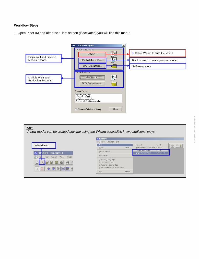
Workflow Steps 1. Open PipeSIM and after the “Tips” screen (if activated) you will find this menu:

Self explanatory

Blank screen to create your own model

1. Select Wizard to build the Model

Multiple Wells and Production Systems

Single well and Pipeline Models Options

SchlumbergerPrivate

Wizard Icon

Tips: A new model can be created anytime using the Wizard accessible in two additional ways:

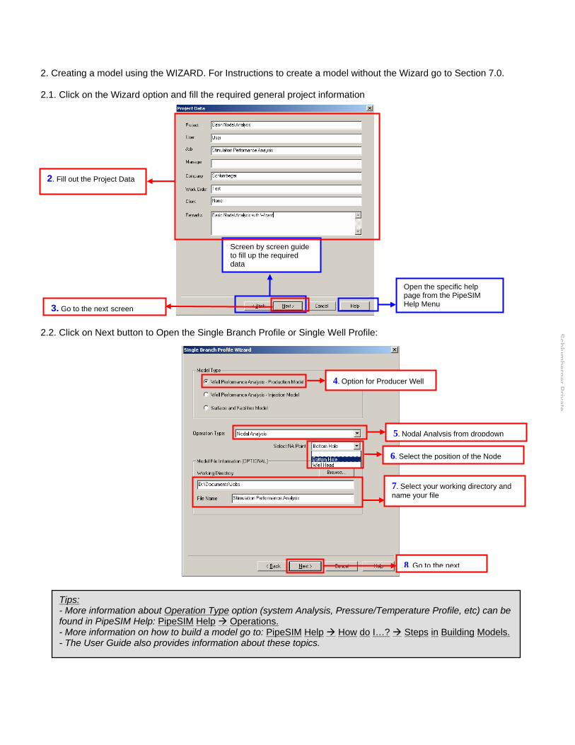
2. Creating a model using the WIZARD. For Instructions to create a model without the Wizard go to Section 7.0. 2.1. Click on the Wizard option and fill the required general project information

Screen by screen guide to fill up the required data

2. Fill out the Project Data

3. Go to the next screen

Open the specific help page from the PipeSIM Help Menu

2.2. Click on Next button to Open the Single Branch Profile or Single Well Profile: SchlumbergerPrivate

8. Go to the next

7. Select your working directory and name your file

6. Select the position of the Node

5. Nodal Analysis from dropdown

4. Option for Producer Well

Tips: - More information about Operation Type option (system Analysis, Pressure/Temperature Profile, etc) can be found in PipeSIM Help: PipeSIM Help Operations. - More information on how to build a model go to: PipeSIM Help How do I…? Steps in Building Models. - The User Guide also provides information about these topics.

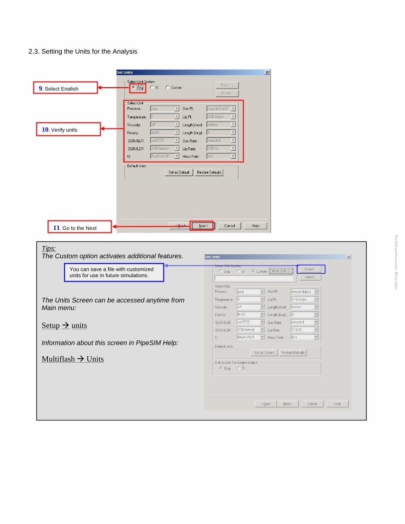
2.3. Setting the Units for the Analysis

11. Go to the Next

10. Verify units

9. Select English

SchlumbergerPrivate

Tips: The Custom option activates additional features. The Units Screen can be accessed anytime from Main menu: Setup units Information about this screen in PipeSIM Help: Multiflash Units

You can save a file with customized units for use in future simulations.

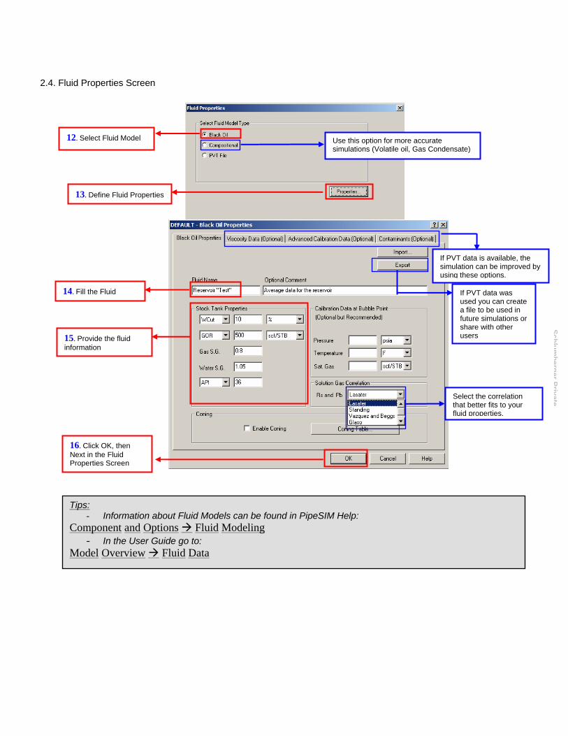
2.4. Fluid Properties Screen

12. Select Fluid Model

SchlumbergerPrivateSelect the correlation

that better fits to your fluid properties.

14. Fill the Fluid

If PVT data is available, the simulation can be improved by using these options.

If PVT data was used you can create a file to be used in future simulations or share with other users15. Provide the fluid

information

Use this option for more accurate simulations (Volatile oil, Gas Condensate)

13. Define Fluid Properties

16. Click OK, then Next in the Fluid Properties Screen

Tips: - Information about Fluid Models can be found in PipeSIM Help:

Component and Options Fluid Modeling - In the User Guide go to:

Model Overview Fluid Data

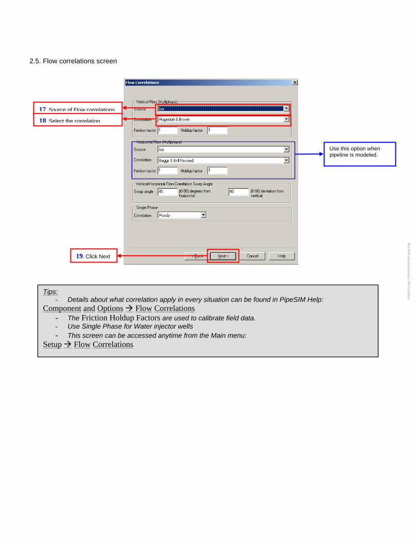
2.5. Flow correlations screen

19. Click Next

Tips: - Details about what correlation apply in every situation can be found in PipeSIM Help:

Component and Options Flow Correlations - The Friction Holdup Factors are used to calibrate field data. - Use Single Phase for Water injector wells - This screen can be accessed anytime from the Main menu:

Setup Flow Correlations

Use this option when pipeline is modeled.

17. Source of Flow correlations

18. Select the correlation

SchlumbergerPrivate

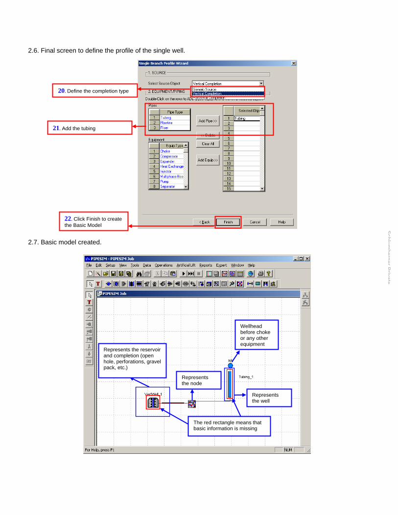
2.6. Final screen to define the profile of the single well.

21. Add the tubing

22. Click Finish to create the Basic Model

20. Define the completion type

SchlumbergerPrivate

2.7. Basic model created.

Represents the node

Wellhead before choke or any other equipment

Represents the reservoir and completion (open hole, perforations, gravel pack, etc.)

The red rectangle means that basic information is missing

Representsthe well

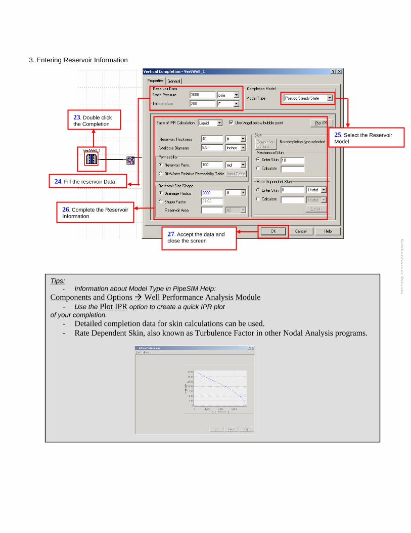
3. Entering Reservoir Information

SchlumbergerPrivate

27. Accept the data and close the screen

23. Double click the Completion

24. Fill the reservoir Data

26. Complete the Reservoir Information

25. Select the Reservoir Model

Tips: - Information about Model Type in PipeSIM Help:

Components and Options Well Performance Analysis Module - Use the Plot IPR option to create a quick IPR plot

of your completion. - Detailed completion data for skin calculations can be used. - Rate Dependent Skin, also known as Turbulence Factor in other Nodal Analysis programs.

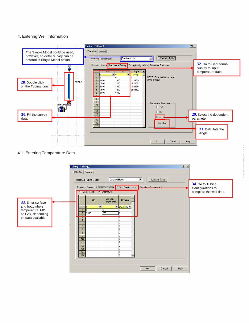
4. Entering Well Information

SchlumbergerPrivate

28. Double click on the Tubing Icon

The Simple Model could be used; however, no detail survey can be entered in Single Model option

31. Calculate the Angle

29. Select the dependent parameter

32. Go to Geothermal Survey to input temperature data.

30. Fill the survey data

4.1. Entering Temperature Data

34. Go to Tubing Configurations to complete the well data.

33. Enter surface and bottomhole temperature. MD or TVD, depending on data available

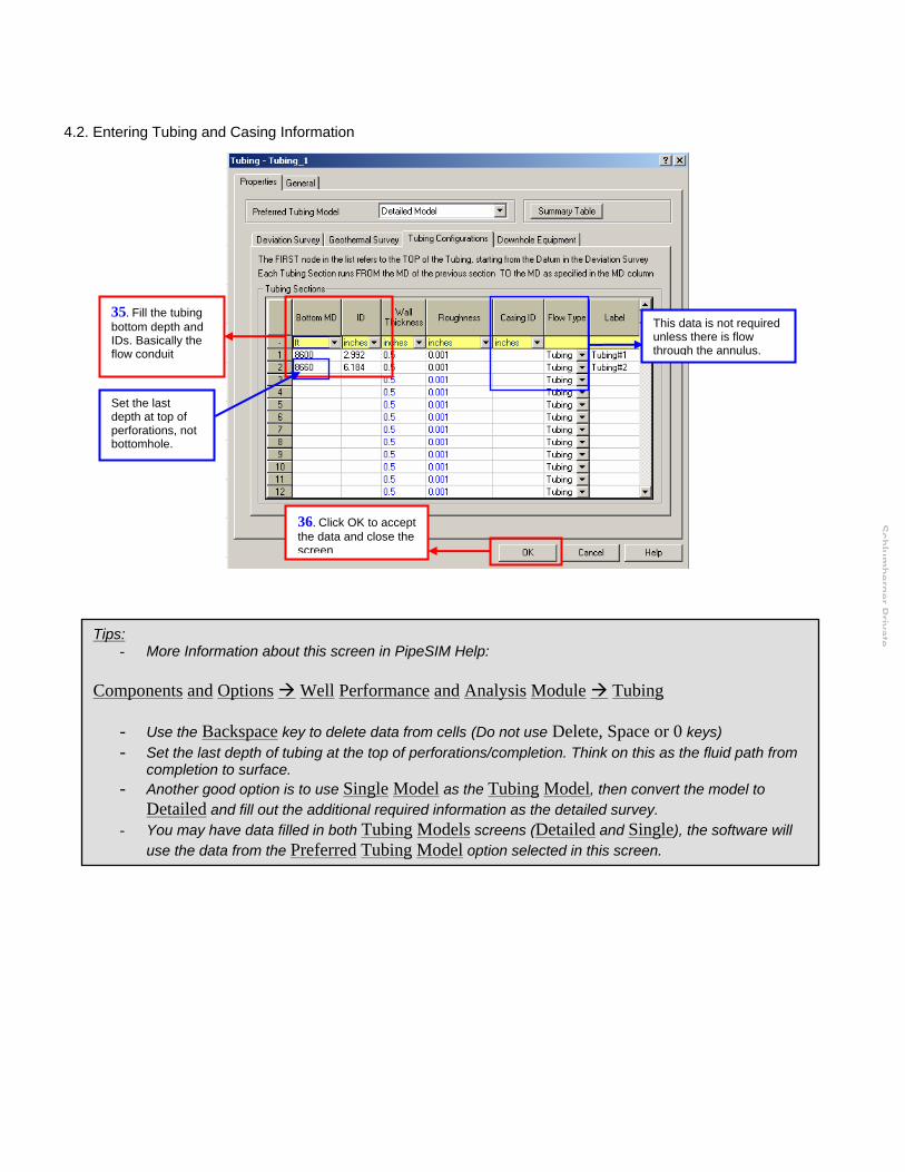
4.2. Entering Tubing and Casing Information

This data is not required unless there is flow through the annulus.

36. Click OK to accept the data and close the screen

35. Fill the tubing bottom depth and IDs. Basically the flow conduit

Set the last depth at top of perforations, not bottomhole.

SchlumbergerPrivate

Tips: - More Information about this screen in PipeSIM Help:

Components and Options Well Performance and Analysis Module Tubing

- Use the Backspace key to delete data from cells (Do not use Delete, Space or 0 keys) - Set the last depth of tubing at the top of perforations/completion. Think on this as the fluid path from

completion to surface. - Another good option is to use Single Model as the Tubing Model, then convert the model to

Detailed and fill out the additional required information as the detailed survey. - You may have data filled in both Tubing Models screens (Detailed and Single), the software will

use the data from the Preferred Tubing Model option selected in this screen.

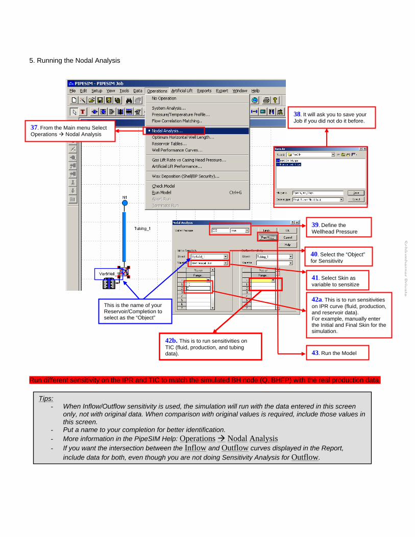
5. Running the Nodal Analysis

SchlumbergerPrivate

Run different sensitivity on the IPR and TIC to match the simulated BH node (Q, BHFP) with the real production data.

37. From the Main menu Select Operations Nodal Analysis

39. Define the Wellhead Pressure

40. Select the “Object” for Sensitivity

41. Select Skin as variable to sensitize

42a. This is to run sensitivities on IPR curve (fluid, production, and reservoir data). For example, manually enter the Initial and Final Skin for the simulation.

43. Run the Model

This is the name of your Reservoir/Completion to select as the “Object”

42b. This is to run sensitivities on TIC (fluid, production, and tubing data).

Tips: - When Inflow/Outflow sensitivity is used, the simulation will run with the data entered in this screen

only, not with original data. When comparison with original values is required, include those values in this screen.

- Put a name to your completion for better identification. - More information in the PipeSIM Help: Operations Nodal Analysis - If you want the intersection between the Inflow and Outflow curves displayed in the Report,

include data for both, even though you are not doing Sensitivity Analysis for Outflow.

38. It will ask you to save your Job if you did not do it before.

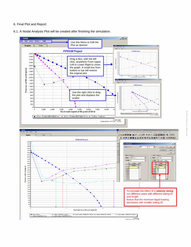
6. Final Plot and Report 6.1. A Nodal Analysis Plot will be created after finishing the simulation.

Use this Menu to Edit the Plot as desired

Drag a Box, with the left click, anywhere From Upper Left to Lower Right to zoom the graph. A small box from bottom to top will restore the original plot

Use the right click to drag the plot and displace the scales

SchlumbergerPrivate

To simulate the effect of a velocity string, run different cases with different tubing ID and length. Notice that the minimum liquid loading decreases with smaller tubing ID.

6.2. Go back to the Main Screen and Select the options: Reports User Reports (Nodal Analysis)

44. Select the User Defined Report option

45. Select the Report Options and Click OK

SchlumbergerPrivate

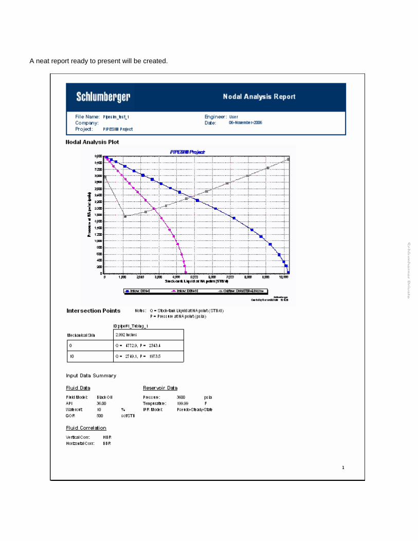
A neat report ready to present will be created.

SchlumbergerPrivate

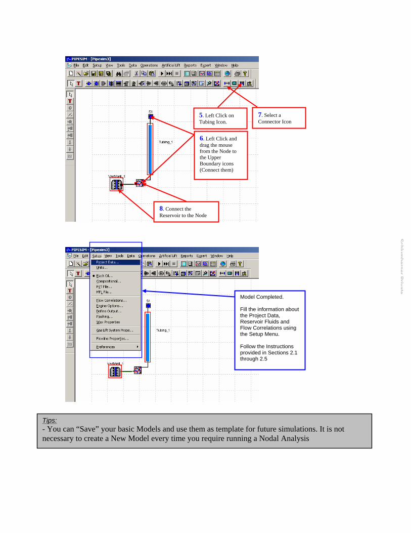
7. Building a Model Without the “Wizard”. Start with a Blank Screen selecting the New Single Branch Model Option

1. Left Click on the Vertical Completion Icon (Do not drag)

2. Left Click on any spot on the screen. The vertical completion will show up

3. Do the same with the Boundary Node

4. And the Node for the Nodal Analysis at bottomhole

SchlumbergerPrivate

SchlumbergerPrivate

5. Left Click on Tubing Icon.

6. Left Click and drag the mouse from the Node to the Upper Boundary icons (Connect them)

7. Select a Connector Icon

8. Connect the Reservoir to the Node

Model Completed.

about

g

ill the information F

the Project Data, Reservoir Fluids and Flow Correlations usinthe Setup Menu.

ollow the Instructions Fprovided in Sections 2.1through 2.5

Tips: can “Save” your basic Models and use them as template for future simulations. It is not - You

necessary to create a New Model every time you require running a Nodal Analysis

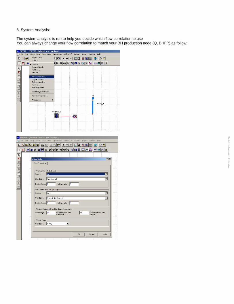
8. System Analysis: The system analysis is run to help you decide which flow correlation to use You can always change your flow correlation to match your BH production node (Q, BHFP) as follow:

SchlumbergerPrivate

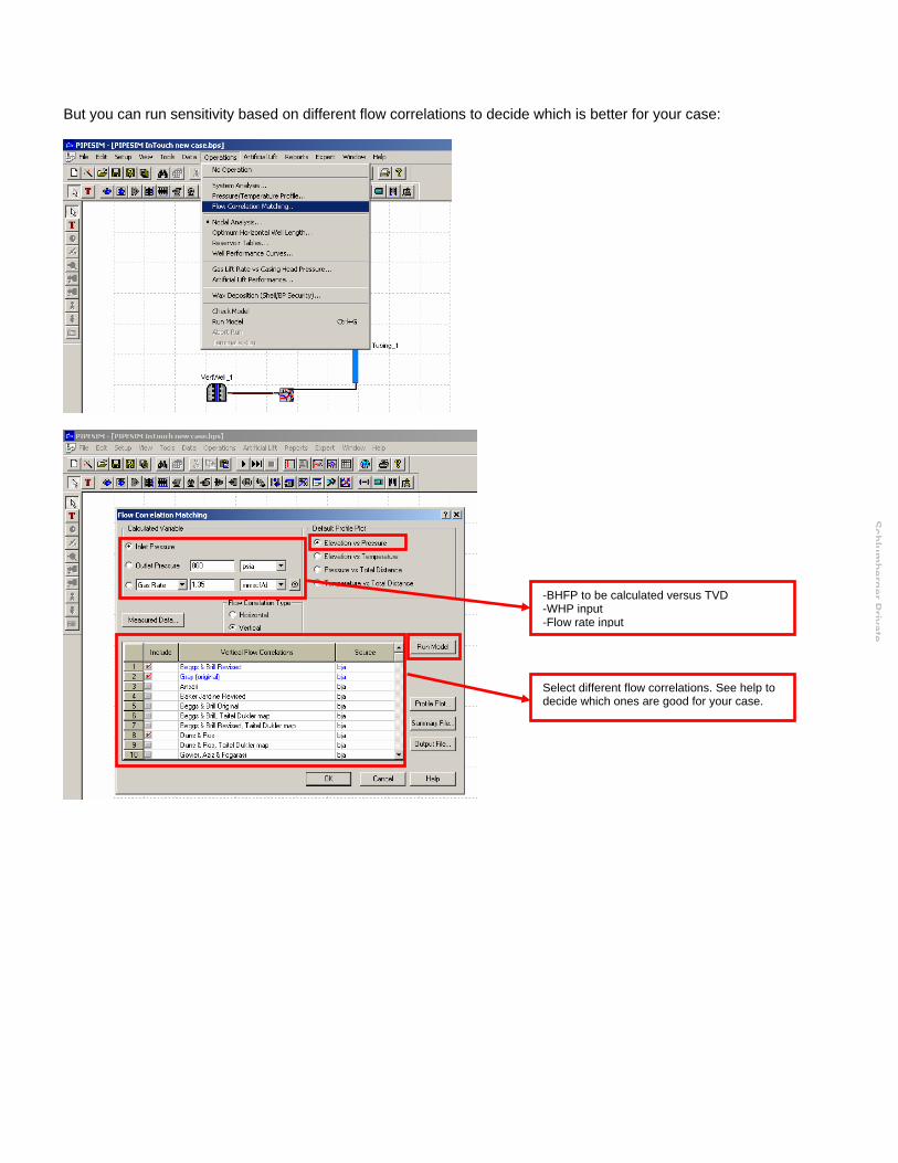
But you can run sensitivity based on different flow correlations to decide which is better for your case:

SchlumbergerPrivate

-BHFP to be calculated versus TVD -WHP input -Flow rate input

Select different flow correlations. See help to decide which ones are good for your case.

SchlumbergerPrivate

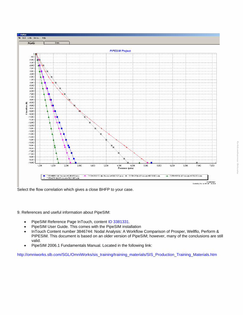
Select the flow correlation which gives a close BHFP to your case. 9. References and useful information about PipeSIM:

• PipeSIM Reference Page InTouch, content ID 3381331. • PipeSIM User Guide. This comes with the PipeSIM installation • InTouch Content number 3846744: Nodal Analysis: A Workflow Comparison of Prosper, Wellflo, Perform &

PIPESIM. This document is based on an older version of PipeSIM; however, many of the conclusions are still valid.

• PipeSIM 2006.1 Fundamentals Manual. Located in the following link: http://omniworks.slb.com/SGL/OmniWorks/sis_training/training_materials/SIS_Production_Training_Materials.htm