How to get cool in the heat: comparing analytic models of ... · 2 THE EAGLE SIMULATIONS AND DATA...
19
MNRAS 467, 2066–2084 (2017) doi:10.1093/mnras/stx243 Advance Access publication 2017 January 30 How to get cool in the heat: comparing analytic models of hot, cold and cooling gas in haloes and galaxies with EAGLE Adam R. H. Stevens, 1‹ Claudia del P. Lagos, 2, 3 Sergio Contreras, 4 Darren J. Croton, 1 Nelson D. Padilla, 4, 5 Matthieu Schaller, 6 Joop Schaye 7 and Tom Theuns 6 1 Centre for Astrophysics and Supercomputing, Swinburne University of Technology, Hawthorn, VIC 3122, Australia 2 International Centre for Radio Astronomy Research, The University of Western Australia, Crawley, WA 6009, Australia 3 Australian Research Council Centre of Excellence for All-sky Astrophysics (CAASTRO), Redfern, NSW 2016, Australia 4 Instituto de Astrof´ ısica, Pontificia Universidad Cat´ olica de Chile, 782-0436 Macul, Santiago, Chile 5 Centro de Astro-Ingenier´ ıa, Pontificia Universidad Cat´ olica de Chile, 782-0436 Macul, Santiago, Chile 6 Institute for Computational Cosmology, Durham University, Durham DH1 3LE, UK 7 Leiden Observatory, Leiden University, NL-2300 RA Leiden, the Netherlands Accepted 2017 January 26. Received 2017 January 24; in original form 2016 August 12 ABSTRACT We use the hydrodynamic, cosmological EAGLE simulations to investigate how the hot gas in haloes condenses to form and grow galaxies. We select haloes from the simulations that are actively cooling and study the temperature, distribution and metallicity of their hot, cold and transitioning ‘cooling’ gas, placing these in the context of semi-analytic models. Our selection criteria lead us to focus on Milky Way-like haloes. We find that the hot-gas density profiles of the haloes form a progressively stronger core over time, the nature of which can be captured by a β profile that has a simple dependence on redshift. In contrast, the hot gas that will cool over a time-step is broadly consistent with a singular isothermal sphere. We find that cooling gas carries a few times the specific angular momentum of the halo and is offset in spin direction from the rest of the hot gas. The gas loses ∼60 per cent of its specific angular momentum during the cooling process, generally remaining greater than that of the halo, and it precesses to become aligned with the cold gas already in the disc. We find tentative evidence that angular-momentum losses are slightly larger when gas cools on to dispersion-supported galaxies. We show that an exponential surface density profile for gas arriving on a disc remains a reasonable approximation, but a cusp containing ∼20 per cent of the mass is always present, and disc scale radii are larger than predicted by a vanilla Fall & Efstathiou model. These scale radii are still closely correlated with the halo spin parameter, for which we suggest an updated prescription for galaxy formation models. Key words: ISM: evolution – ISM: structure – galaxies: evolution – galaxies: formation – galaxies: haloes – intergalactic medium. 1 INTRODUCTION Fundamentally, galaxies must form from the cooling and conden- sation of gas residing in overdense regions of the Universe (e.g. White & Rees 1978). The manner in which the gas is accreted over cosmic time is vital to the structure of a galaxy and how it evolves. This is especially true for late-type galaxies, where discs hold the majority of a galaxy’s baryonic mass, and when considering the high-redshift Universe, prior to mergers dominating the growth of the most massive galaxies. E-mail: [email protected] The semi-analytic approach of galaxy formation (White & Frenk 1991; Kauffmann, White & Guiderdoni 1993; Cole et al. 1994; Kauffmann et al. 1999; see reviews by Baugh 2006; Somerville & Dav´ e 2015) provides a framework that is consis- tent with the hierarchical assembly of overdense regions, known as haloes. Here, the histories and properties of dark matter haloes formed in a cosmological N-body simulation provide the input for the coupled differential equations that describe the evolution of galaxies. These computationally efficient models have proven highly successful in their ability to reproduce the statistical prop- erties of galaxies in the local Universe and are becoming progres- sively more successful in the early Universe (e.g. Gonzalez-Perez et al. 2014; Henriques et al. 2015; Lacey et al. 2016). C 2017 The Authors Published by Oxford University Press on behalf of the Royal Astronomical Society
Transcript of How to get cool in the heat: comparing analytic models of ... · 2 THE EAGLE SIMULATIONS AND DATA...

MNRAS 467, 2066–2084 (2017) doi:10.1093/mnras/stx243Advance Access publication 2017 January 30
How to get cool in the heat: comparing analytic models of hot, coldand cooling gas in haloes and galaxies with EAGLE
Adam R. H. Stevens,1‹ Claudia del P. Lagos,2,3 Sergio Contreras,4 Darren J. Croton,1
Nelson D. Padilla,4,5 Matthieu Schaller,6 Joop Schaye7 and Tom Theuns6
1Centre for Astrophysics and Supercomputing, Swinburne University of Technology, Hawthorn, VIC 3122, Australia2International Centre for Radio Astronomy Research, The University of Western Australia, Crawley, WA 6009, Australia3Australian Research Council Centre of Excellence for All-sky Astrophysics (CAASTRO), Redfern, NSW 2016, Australia4Instituto de Astrofısica, Pontificia Universidad Catolica de Chile, 782-0436 Macul, Santiago, Chile5Centro de Astro-Ingenierıa, Pontificia Universidad Catolica de Chile, 782-0436 Macul, Santiago, Chile6Institute for Computational Cosmology, Durham University, Durham DH1 3LE, UK7Leiden Observatory, Leiden University, NL-2300 RA Leiden, the Netherlands
Accepted 2017 January 26. Received 2017 January 24; in original form 2016 August 12
ABSTRACTWe use the hydrodynamic, cosmological EAGLE simulations to investigate how the hot gasin haloes condenses to form and grow galaxies. We select haloes from the simulations thatare actively cooling and study the temperature, distribution and metallicity of their hot, coldand transitioning ‘cooling’ gas, placing these in the context of semi-analytic models. Ourselection criteria lead us to focus on Milky Way-like haloes. We find that the hot-gas densityprofiles of the haloes form a progressively stronger core over time, the nature of which canbe captured by a β profile that has a simple dependence on redshift. In contrast, the hot gasthat will cool over a time-step is broadly consistent with a singular isothermal sphere. We findthat cooling gas carries a few times the specific angular momentum of the halo and is offset inspin direction from the rest of the hot gas. The gas loses ∼60 per cent of its specific angularmomentum during the cooling process, generally remaining greater than that of the halo, andit precesses to become aligned with the cold gas already in the disc. We find tentative evidencethat angular-momentum losses are slightly larger when gas cools on to dispersion-supportedgalaxies. We show that an exponential surface density profile for gas arriving on a disc remainsa reasonable approximation, but a cusp containing ∼20 per cent of the mass is always present,and disc scale radii are larger than predicted by a vanilla Fall & Efstathiou model. These scaleradii are still closely correlated with the halo spin parameter, for which we suggest an updatedprescription for galaxy formation models.
Key words: ISM: evolution – ISM: structure – galaxies: evolution – galaxies: formation –galaxies: haloes – intergalactic medium.
1 IN T RO D U C T I O N
Fundamentally, galaxies must form from the cooling and conden-sation of gas residing in overdense regions of the Universe (e.g.White & Rees 1978). The manner in which the gas is accreted overcosmic time is vital to the structure of a galaxy and how it evolves.This is especially true for late-type galaxies, where discs hold themajority of a galaxy’s baryonic mass, and when considering thehigh-redshift Universe, prior to mergers dominating the growth ofthe most massive galaxies.
� E-mail: [email protected]
The semi-analytic approach of galaxy formation (White &Frenk 1991; Kauffmann, White & Guiderdoni 1993; Coleet al. 1994; Kauffmann et al. 1999; see reviews by Baugh 2006;Somerville & Dave 2015) provides a framework that is consis-tent with the hierarchical assembly of overdense regions, known ashaloes. Here, the histories and properties of dark matter haloesformed in a cosmological N-body simulation provide the inputfor the coupled differential equations that describe the evolutionof galaxies. These computationally efficient models have provenhighly successful in their ability to reproduce the statistical prop-erties of galaxies in the local Universe and are becoming progres-sively more successful in the early Universe (e.g. Gonzalez-Perezet al. 2014; Henriques et al. 2015; Lacey et al. 2016).
C© 2017 The AuthorsPublished by Oxford University Press on behalf of the Royal Astronomical Society

How to get cool in the heat 2067
Many of the semi-analytic models in the literature (e.g. Coleet al. 2000; Hatton et al. 2003; Croton et al. 2006, 2016; Lagos,Cora & Padilla 2008; Somerville et al. 2008b; Guo et al. 2011;Benson 2012) have been, in part, based on the disc formation sce-nario developed by Fall & Efstathiou (1980) and Mo, Mao & White(1998). In these models, it is assumed that halo gas (the circum-galactic or intracluster medium) has a uniform temperature andcarries the same total specific angular momentum as the halo (vari-ants have adopted a statistical take on spin direction – see Padillaet al. 2014; Lagos et al. 2015a). Two regimes of gas accretion onto galaxies are typically employed. For the ‘hot mode’, infallinggas is first shock heated to the virial temperature, then must coolto reach the galaxy. In the ‘cold mode’, the cooling time-scale issmall relative to the free-fall time-scale, and hence the former nolonger sets the time-scale for accretion (see White & Frenk 1991;Birnboim & Dekel 2003; Keres et al. 2005; Benson & Bower 2011).When the gas condenses on to a disc, it is assumed to conserve itsspecific angular momentum, and to settle with a surface densitythat decreases exponentially with radius. Often rotation curves ofdiscs are approximated as completely flat. Variants also includeexponential cooling profiles as a function of specific angular mo-mentum (Stevens, Croton & Mutch 2016). While these assumptionsall carry physical merit, like anything, they would ideally be subjectto independent testing.
With this study, we are motivated to investigate the basic as-sumptions of the aforementioned models with respect to the hotmode of accretion. That is, how is hot gas distributed in haloes,what is the nature and distribution of gas as it cools on to a galaxyand does this gas conserve its specific angular momentum? Theseare not only important science questions in and of themselves, butanswers to these have a direct impact on galaxy evolution modeldevelopment. To address these topics with modern observationswould be an unsurmountable challenge. In this sense, we cannottruly test the model assumptions. We can, however, look to numer-ical experiments with more detailed physics for an insight, namelyhydrodynamic cosmological simulations. This allows us to see howthe widely adopted theoretical description of gas cooling on globalscales (Fall & Efstathiou 1980; White & Frenk 1991) comparesto predictions from modelling galaxy evolution physics on local(�kpc) scales. Hydrodynamic simulations also carry the advantagethat we can immediately relate any results regarding gas cooling tothe properties of dark matter haloes.
We use the EAGLE simulations (Evolution and Assembly ofGaLaxies and their Environments; Crain et al. 2015; Schayeet al. 2015) to study the gas particles in haloes that cool from ahot state down on to galaxies. We assess how these particles aredistributed in physical space and in terms of specific angular mo-mentum both prior to and after cooling episodes. We compare thisagainst the overall hot and cold gas profiles in haloes, investigatinghow the process of cooling leads to evolution in these structures.We further determine whether the angular momentum of these par-ticles is conserved as they cool, both on an individual basis andas a collective system. EAGLE provides an ideal testbed to ad-dress these questions, as there is growing evidence the simulationproduces a realistic galaxy population in terms of mass (Furlonget al. 2015), size (Furlong et al. 2017), specific angular momen-tum (Lagos et al. 2017) and gas content (Lagos et al. 2015b; Baheet al. 2016).
Recently, Guo et al. (2016) compared the galaxy populations oftwo semi-analytic models, run on the dark-matter-only halo mergertrees of EAGLE, against the main hydrodynamic EAGLE simula-tion. Those authors found consistency in the evolution of the stellar
mass function and the specific star formation rates of galaxies, butnoted clear differences when galaxies were broken into passive andstar-forming. However, their study did not address whether the phys-ical description and approximations of galaxy evolution processesin the semi-analytic models were supported by hydrodynamic sim-ulations. Our study contributes by focusing on the physics of themodels, rather than testing whether the end results, i.e. the galaxyproperties, are in agreement with each other or observations.
While we address aspects of models of halo gas cooling in thispaper, our focus has intentionally not been placed on raw coolingrates. Comparisons of cooling rates in hydrodynamic simulationsand semi-analytic models have already been the focus of papers inthe past (Lu et al. 2011; Monaco et al. 2014). A major challengefor these types of studies is the complex interplay between coolingand feedback, and the differing techniques for implementing this inhydrodynamic simulations and semi-analytic models. For example,a semi-analytic model must explicitly distinguish between feedbackthat reheats cold gas and feedback that suppresses the cooling of hotgas (see e.g. Croton et al. 2006), which might instead be implicit ina hydrodynamic simulation. Furthermore, the knowledge that gashas been reheated is typically not maintained in a semi-analyticmodel, yet hydrodynamic simulations have shown that the samegas particles can be reheated and cool on to the same galaxy manytimes (Christensen et al. 2016; also see Oppenheimer et al. 2010;Ford et al. 2014). This adds challenges related to time resolution forextracting the true cooling rates of haloes from the snapshot dataof hydrodynamic simulations. As a result of all this, feedback hasbeen favourably omitted for the aforementioned comparison studies,which hence assess idealized, rather than physical, cooling rates. Inlight of these challenges, but with a different method of approach, wecompare semi-analytic-equivalent cooling rates of EAGLE haloesusing their full structural information from the simulations versusthe standard method of using their global properties. A completestudy of the physical cooling rates of EAGLE haloes is worthy of apaper by itself, and thus we leave that for future work.
This paper is structured as follows. In Section 2, we provide de-tails on the design of the EAGLE simulations and the data productsthat we have used. We also specify the sample of galaxies withinthe simulations that we study. In Section 3, we examine the stateof hot gas in haloes, comparing this to the particles that are aboutto cool. In Section 4, we discuss the direction and magnitude, withrespect to the halo, of the specific angular momentum of gas asit cools, and whether this is conserved. Once those particles havecooled on to a disc, we study their distribution, and that of the discin full, in Section 5. The results of this paper are then summarizedin Section 6.
Throughout this paper, where relevant, we assume the cosmologyused in the EAGLE simulations (see Section 2). We also use the term‘virial radius’ as the radius enclosing an average density 200 timesgreater than the critical density of the Universe, i.e. Rvir = R200,Mvir = M200 = M(<R200). We use capital R for three-dimensionalradial distances (R2 = x2 + y2 + z2) and lowercase r for two-dimensional equivalents (r2 = x2 + y2, where the z-direction isalways parallel to the relevant rotation axis).
2 TH E E AG L E SI M U L ATI O N S A N D DATA
2.1 Overview of the simulations
The EAGLE simulations are a suite of state-of-the-art hydrody-namic, cosmological simulations, first presented by Schaye et al.(2015). They were run using a significantly modified version of
MNRAS 467, 2066–2084 (2017)
2068 A. R. H. Stevens et al.
GADGET3, an N-body Tree-PM smoothed particle hydrodynamics(SPH) code. Various modifications of GADGET have been devel-oped by the community. The most recent official public releasewas GADGET2 (Springel 2005). The simulations assumed a �CDMcosmology with parameters based on the 2013 Planck data release:�M = 0.307, �� = 0.693, �b = 0.048, h = 0.6777, σ 8 = 0.8288and ns = 0.9611 (Planck Collaboration XVI 2014). The main ‘Refer-ence’ simulation used a dark matter particle mass of 9.70 × 10⁶ M�,an initial gas particle mass of 1.81 × 10⁶ M�, and a Plummer-equivalent gravitational softening scale of 2.66 comoving kpc forz > 2.8 and 700 physical pc otherwise. The simulations imple-mented a modified version of SPH, dubbed ANARCHY (Dalla Vec-chia, in preparation; but see appendix A of Schaye et al. 2015),along with the time-step limiter of Durier & Dalla Vecchia (2012).Schaller et al. (2015b) presented a comparison of the simulationswith the old SPH version, and found that the modifications wereimportant for active galactic nucleus (AGN) activity and star for-mation rates of large galaxies, but, by and large, did not have a bigimpact on stellar masses and sizes.
The simulations include a set of sub-grid models that describephysical processes below the resolution limit. These are describedin full in Schaye et al. (2015). Briefly, these include the following.
(i) Radiative cooling of gas particles is calculated by follow-ing 11 elements (Wiersma, Schaye & Smith 2009a), which areassumed to be in ionization equilibrium. Gas is exposed to the cos-mic microwave background, and after z = 11.5, a uniform ionizingbackground is included (Haardt & Madau 2001). Self-shielding andlocal stellar radiation are ignored.
(ii) Star formation is based on the local pressure of gas (Schaye& Dalla Vecchia 2008) and is consistent with the Kennicutt–Schmidt relation (Kennicutt 1998). This is triggered only abovea threshold local density, which has a metallicity-dependent value(Schaye 2004). Star particles are each considered to be single stel-lar populations that follow the initial mass function of Chabrier(2003) and the stellar evolution models described by Wiersma et al.(2009b). Stellar feedback from supernovae is implemented with thestochastic thermal model of Dalla Vecchia & Schaye (2012).
(iii) Black-hole particles of mass 105 h−1 M� are seeded inhaloes once they reach a mass of 1010 h−1 M� (Springel, Di Matteo& Hernquist 2005). These accrete gas from neighbouring particles,with a consideration of angular momentum as in Rosas-Guevaraet al. (2015), which leads to AGN feedback where nearby gas par-ticles are stochastically heated (Schaye et al. 2015).
The free parameters of the sub-grid physics in EAGLE werecalibrated to best reproduce a small number of key observables ofgalaxies in the local (z ∼ 0) Universe: the stellar mass function (Li& White 2009; Baldry et al. 2012), the stellar size–mass relationof Shen et al. (2003) and the black hole–stellar mass relation ofMcConnell & Ma (2013). See Crain et al. (2015) for further details.
In this paper, in addition to the Reference simulation, we also useruns with modified feedback physics but equal resolution. Theseinclude runs with stellar feedback half the Reference strength(WeakFB), stellar feedback with twice the Reference strength(StrongFB), and an absence of AGN feedback (NoAGN). We alsouse the high-resolution run of EAGLE (with eight-fold superiormass resolution), for which the strength of feedback was recal-ibrated to meet the same observational constraints as mentionedabove (RecalHR). The alternate-feedback and high-resolution runswere performed in 25-Mpc boxes. As we want to fairly comparethese to Reference haloes, we use the 25-Mpc Reference simulation
for this paper as well. Further details on these simulations can alsobe found in Crain et al. (2015).
2.2 Halo finding
To identify structures in EAGLE, SUBFIND (Springel et al. 2001;Dolag et al. 2009) was run on the output of the simulations. Forthe purposes of the code, a ‘halo’ is a collection of particles foundwith a friends-of-friends algorithm. A ‘subhalo’ is a set of parti-cles in a halo that is enclosed by isodensity contours that traversesaddle points, where only particles gravitationally bound to thesubstructure are included. A subhalo encompasses a galaxy and itsimmediate surroundings. All haloes have a minimum of one sub-halo (haloes with more than one subhalo have satellite galaxies).Neither haloes nor subhaloes are inherently restricted to their virialradii (we specify when only particles within Rvir are considered).Note that all results in this paper concerning ‘haloes’ consider onlythe primary subhalo.
2.3 Galaxy sample selection
For the purposes of this paper, we are interested in studying haloesundergoing cooling episodes. To identify a relevant sample of sys-tems in EAGLE, first we select central subhaloes (most massivein their parent halo) with total gas masses >109.5 M�, then wecompare the state of gas particles of the same IDs at temporallyadjacent snapshots within each subhalo. More specifically, we takeeach relevant subhalo at snapshot number s and tabulate the IDsof all particles we consider ‘hot’. We then find the same particlesat snapshot s + 1 and determine which of these are now ‘cold’and within the same system. Those that have transitioned from hotto cold, or from hot to a star particle, from snapshot s to s + 1are labelled ‘cooled’ particles. Equivalently, we refer to these as‘cooling’ particles at snapshot s. If the number of cooling particlesexceeds a threshold value (64, see below), then we deem a resolvedcooling episode to have happened and include that subhalo in oursample. We perform this same process for all snapshot pairs.
Note that in order to have a clean sample of central galaxies tocompare against how semi-analytic models treat centrals, we ex-clude galaxies from our analysis that are satellites at either snapshot(that is, we consider only the primary subhalo of each halo). Wefurther exclude galaxies that undergo a major merger between snap-shots. We define a major merger as one where the smaller galaxyhas a stellar mass at least 30 per cent that of the central. Thesewould have constituted only a small fraction of our sample. Assuch, had we included them, our results would not have noticeablychanged. When selecting haloes from the alternate-feedback andhigh-resolution runs, we add a requirement that only haloes alsopresent in the Reference sample can be included.
Throughout this text, we define ‘cold’ particles as either havingnon-zero star formation rates or having both temperature T < 104.5 Kand hydrogen number density nH > 0.01 cm−3, which should cap-ture the interstellar medium of most galaxies. Conversely, ‘hot’ gasparticles have zero star formation rates and T > 105 K.
A cooling episode should occur over a time-span comparable tothe dynamical time of a halo, which is directly tied to the Hubbleflow at the given redshift:
tdyn = Rvir/Vvir = [10 H (z)]−1 , (1)
where Rvir and Vvir are the virial radius and velocity, respectively, ofa given halo. As we want to capture the before and after states of acooling episode, snapshots separated by a dynamical time would be
MNRAS 467, 2066–2084 (2017)

How to get cool in the heat 2069
Figure 1. Ratio of a halo dynamical time at the redshift of snapshot numbers to the time to the next snapshot in EAGLE. Snapshots to the right-handside of the vertical dotted line were included in the analysis of this paper.
Figure 2. Normalized histograms of masses of Reference EAGLE systemsused in this paper, according to the selection criteria given in Section 2.3. Thesolid distributions give the haloes’ virial masses. The dashed and dot–dasheddistributions give the gas and stellar masses, respectively, of all particles inthe main subhalo within Rvir. Each panel covers a different redshift range,as labelled, with the same number of snapshots.
well suited for our study. By no coincidence, the temporal separationbetween snapshots in EAGLE never differs from a dynamical timeby more than ∼40 per cent (with the exception of the first twosnapshots in the simulation, which we do not use in this paper).This is illustrated by Fig. 1.
The precise threshold imposed for the minimum number of cool-ing particles is, at some level, arbitrary. A threshold is required toavoid numerical noise and to ensure a meaningful mass cools. Wefind a round value of 64 particles returns a sizeable number of haloes(an average of 48 per snapshot interval in the 25-Mpc box), eachwith sizeable cooling rates (�0.2 M� yr−1). Of course, the truecooling rates of haloes over each snapshot interval can be higher, asthere may have been particles that cooled and were reheated withinthe interval that we missed. It is possible then that our results arebiased towards higher-mass systems with high cooling rates, andcaution should be heeded when extrapolating to lower masses (seeFig. 2 and below). By comparing the recorded historical maximumtemperature of gas particles before and after cooling in our sample,we know that the ratio of hot particles that cool and are reheatedbetween snapshots is, in the majority of cases, small compared to
those that cool and remain cold, but it is difficult to quantify exactlywhich particles have been affected by feedback (beyond those di-rectly injected with energy) with snapshot data. As will be shown,our 64-particle threshold leads to results that are consistent with theRecalHR simulation when we select the same haloes. We are, how-ever, restricted to studying haloes at z < 4. The average temporalseparation between snapshots in this range is 681 Myr.
We present the masses of our sample of Reference EAGLE haloesin Fig. 2. We break these into three redshift bins, each with sixsnapshot pairs, which we use throughout this paper. The normalizedhistograms show the virial masses of the haloes, as well as the gasand stellar masses of all particles in each respective main subhaloinside an aperture of Rvir. Note that the gas masses are for all gas,i.e. hot + cold + everything in between.
3 B E F O R E C O O L I N G : H OT G A S I N H A L O E S
3.1 Temperature profiles of hot gas
In the absence of cold streams, before finding itself in a galaxy, gaswill find itself in a hot state, sitting in a halo. Models of galaxyevolution often operate under the assumption that the hot gas inhaloes, and therefore the hot gas that will cool, carries a uniformtemperature that is equal to the virial temperature. To compareagainst this, we examine the temperature profiles of haloes in ourEAGLE sample, each normalized by its virial temperature. Thevirial temperature is given by
Tvir = μmp
2kBV 2
vir = 35.9
(Vvir
km s−1
)2
K, (2)
where kB is the Boltzmann constant, and we have adopted a meanmolecular weight, μmp, of 59 per cent that of the proton mass.
We present temperature profiles of hot gas from our sample ofEAGLE haloes from the Reference and RecalHR runs in the toppanels of Fig. 3. The profiles were built by measuring the meantemperature of hot gas particles within spherical shells. We use (amaximum of) 100 shells for each halo, where each shell encom-passes the same number of particles for a given halo, unless thatwidth is below the spatial resolution (softening scale) of the simu-lation. We show the evolution of these profiles by grouping systemsinto three redshift bins, where each bin includes the same numberof snapshots. We display profiles for the median and 16th–84th per-centile range of our samples in Fig. 3. It is immediately clear thatthe hot gas is not truly isothermal, but rather the temperature tendsto decrease with radius. At higher redshift, the gas is within a factorof ∼2 of being isothermal and approaches Tvir towards the centre.As time evolves, the centres become hotter and the temperaturegradient steepens.
The bottom panels in Fig. 3 consider only the hot gas that willcool (on to the galaxy) before the subsequent snapshot, which wedub ‘cooling’ particles. As these particles constitute only a smallfraction of the hot gas, we reduce the number of spherical shellsto 20 in each halo for measuring these profiles. Tcooling(R) has aclear gradient from a high redshift onwards. This shows that gasthat settles on to a galaxy from a larger distance tends to alreadybe cooler than the inner gas. Physically, this makes sense, as gasat large radii is at a lower density (see below) and hence has lessopportunity to lose its energy through collisions over the same time.It is not surprising that the average temperature of cooling gas isconsistently below the hot gas in general; the hotter particles wouldrequire longer to cool. Perhaps what is more interesting is that asthe centres of haloes heat overall, the temperature of the cooling
MNRAS 467, 2066–2084 (2017)

2070 A. R. H. Stevens et al.
Figure 3. Temperature profiles of non-star-forming, hot (T > 105 K) gas in haloes in the Reference and RecalHR runs of EAGLE. The top row of panelspresents the temperature profiles for all hot gas in the haloes, while the bottom panels include only hot gas particles that are known to cool (on to the galaxy) bythe following snapshot. The temperature in both these cases is normalized by the virial temperature of each halo. Columns of panels are for different redshiftranges. The median (solid and dashed curves) and inner 68 per cent (shaded regions of corresponding colour) of profiles are shown in each panel for the twosimulations. Vertical dashed lines are given at Rvir to indicate the cut-off for what is typically regarded as part of a halo. While the hot-gas temperature rises inthe centre, the gas that cools continues to get cooler.
particles decreases. As discussed further in Section 3.2, the densityof hot gas decreases at the centres of haloes over time (see Fig. 5shown later). This means that there is less opportunity for hot gasto cool through collisions, and thus the temperature difference ofa particle before and after a cooling episode (over a time-step)decreases. Small differences are seen between the Reference andRecalHR runs (which we come back to briefly in Section 4.2), butthey are broadly consistent with each other.
To quantify the effect of feedback on the temperature structureof the hot haloes, we have calculated the same temperature profilesfor the alternate-feedback runs of EAGLE. We present these forthe lowest-redshift bin in Fig. 4, comparing the median profile ofthe Reference simulation to the median, 16th and 84th percentilesof the WeakFB, StrongFB and NoAGN runs. At higher redshift,the profiles of the alternate-feedback runs more closely matchedthose of the Reference run (as they have the same initial condi-tions, and so we have omitted them). The differences seen at lowredshift are hence directly the result of feedback associated withgalaxy evolution. Note that the number of systems meeting ourselection criteria in each run varies as a result of the differingfeedback. This is summarized in Table 1. For our results, we in-clude only the haloes in each sample that are also present in theReference sample.
Let us first examine the role of stellar feedback. Stellar feedbackis implemented thermally in EAGLE. This raises the temperature ofgas particles in the centre of the haloes, where the exploding starsare. These hot particles rise and can drive shocks that heat theirneighbours. In our sample, the masses of the haloes are large enoughthat supernova energy is insufficient to eject gas from galaxies outof the halo entirely. The result instead is that the gradient of thetemperature profile becomes generally steeper. As seen in the toppanel of Fig. 4, the WeakFB run shows lower Thot(R) than theReference simulation across all radii and has a shallower gradient.Meanwhile, the StrongFB run has a stronger gradient, and is notablyhotter towards the centre.
Figure 4. Temperature profiles of hot gas in haloes for various alternate-feedback runs of EAGLE, considering only systems at z < 0.6. The top panelincludes all hot gas in the profiles, while the bottom panel includes only thatwhich is known to cool before the next time-step. The thick, opaque curvesgive the median profiles of the different EAGLE runs. The thin, transparentlines give the 16th and 84th percentiles for the alternate-feedback runs. Thebracketed numbers in the legend indicate the number of haloes in the sampleof each run. Both stellar and AGN feedback affect the temperature profilesof hot haloes, but the gas in the process of cooling is not affected identically.
Comparison of the WeakFB and Reference simulations in thebottom panel of Fig. 4 highlights that less efficient stellar feed-back leads to less massive and less turbulent hot-gas haloes at lowredshift, which reduces the opportunity for cooling, thus loweringTcooling(R). At higher redshift, cooling is still efficient, and due to alack of reheating of this cooled gas, the cooling rates of the WeakFB
MNRAS 467, 2066–2084 (2017)

How to get cool in the heat 2071
Table 1. Number of haloes at z < 0.6 in each samplefrom the various runs of EAGLE. Nhalo is the full numberthat met our selection criteria (Section 2.3). Ncommon isthe number of these haloes that are also in the Referencesample. Only the latter are used in this paper.
Simulation Nhalo Ncommon
Reference 175 175WeakFB 57 30StrongFB 106 106NoAGN 292 140
haloes at low redshift are reduced relative to the Reference run, andhence there are far fewer galaxies in the former’s sample (see Ta-ble 1). Moving from the Reference to the StrongFB run does notchange Tcooling(R) significantly at low z, however. While there ismore hot gas in the case of StrongFB, most of it is at a high enoughtemperature such that it may not mix effectively and does not havesufficient time to cool over a time-step. The temperature signatureof the cooling gas hence remains unchanged. Instead, due to thehaloes being hotter, we find that fewer StrongFB haloes are activelycooling at low redshift versus the Reference run (but more than theWeakFB case), as highlighted in Table 1.
Let us now consider the role of AGNs. Perhaps counter-intuitively, switching AGN off leads to an evolution in Thot(R) thatlooks similar to the StrongFB case (top panel of Fig. 4). While AGNfeedback does heat the central gas particles in a halo, the net effectis less a case of the temperature simply rising at the centre, andmore a case of AGNs regulating the temperature of the gas through-out the haloes. Strong outflows from AGNs advect hot particles tolarger distances from the galaxy than stellar-driven outflows would,thereby spreading the heat out and reducing the temperature gra-dient. In fact, for the haloes common to both the Reference andNoAGN samples, we found that the total baryonic mass within Rvir
for the NoAGN run was higher by ∼0.2–0.3 dex for the low-redshiftbin, implying that AGN outflows were able to eject baryons fromthe haloes. This also helps to explain why there are 67 per cent moreNoAGN haloes that are actively cooling at z < 0.6 compared to theReference run (see Table 1).
The difference between the NoAGN run and the others is thatTcooling(R) also increased throughout the halo (see the bottom panelof Fig. 4). This shows that an AGN suppresses the ability of hotgas to cool, as now, without AGNs, hotter gas is seen to cool moreefficiently. This is precisely how radio-mode AGN feedback is con-sidered in semi-analytic models (e.g. Bower et al. 2006; Crotonet al. 2006); that is, the heating rate of a radio AGN is subtracteddirectly off the cooling rate of a halo to calculate its net coolingrate (see Section 3.5). Although, note that EAGLE does not dis-tinguish between radio and quasar modes of AGNs, instead optingfor a single model of AGN feedback that is more in line with thequasar mode (see Schaye et al. 2015). Even if the net effect of AGNfeedback in EAGLE is to make the cooling process less efficient,one would expect the properties of AGN-driven winds in EAGLEto differ if radio-mode feedback were implemented directly in thesimulation (see Dubois et al. 2012).
If one is to believe the results of the EAGLE simulations, it seemsappropriate for semi-analytic models to treat the effects of stellar andAGN feedback on cooling separately. To summarize more specifi-cally, in Milky Way-mass haloes in EAGLE, stellar feedback heatscold gas but does not prevent fresh gas from cooling, whereas AGNfeedback can eject gas from the halo entirely and more directlyimpacts cooling gas by regulating the temperature structure of the
halo, which can suppress the efficiency of cooling. Ideally, prescrip-tions for feedback effects on cooling in semi-analytic models wouldbe based on observations. Recent efforts to identify signatures offeedback effects on stacked X-ray observations of cooling hot gasaround galaxies have shown consistency with gentle, self-regulatedmechanical AGN feedback in the luminosity–temperature relation(Anderson et al. 2015). Cold-phase studies of the circumgalacticmedia of isolated galaxies have found evidence for replenishmentthrough outflows from stellar feedback (Nielsen et al. 2016), al-though how this might translate into a model for feedback-affectedcooling is yet unclear. As of now, hydrodynamic simulations arethe best tool available for developing coarser models of feedback-affected cooling. While beyond the scope of this paper, we suggestthat the EAGLE simulations would provide a good testbed for thisfollow-up study.
3.2 Density profiles of hot gas
We now turn our attention to the density profiles of hot gas in haloes.Using the same spherical shells as used for the temperature profiles,we measure the density within each shell of our EAGLE haloes.We normalize the density profile of each hot halo by mhot/R
3vir.
We then make the same measurements for the cooling gas, insteadnormalized by mcooling/R
3vir. This allows us to directly compare
the density profiles of both the hot and cooling gas, regardlessof the halo size or total hot/cooling mass. In Fig. 5, we present thesefor the same three redshift bins as before. The top row shows thedensity profiles for all hot gas, while the bottom row is for coolinggas. The Reference and RecalHR runs produce consistent profileswith each other, and any differences to the alternate-feedback runsare similarly small on a logarithmic scale (and hence we have notincluded the profiles for those runs).
A clear evolution is seen in the hot-gas density profiles, where thegradient at the centre becomes shallower with time. The cooling-gasdensity profile evolves less noticeably, however, and remains steep.The fact that cooling is always more effective at the centres of haloeshelps elucidate why the total hot-gas density profile forms a coreover time. While the hot gas at the centre becomes hotter and lessdense (relative to the outer parts of the same halo), the profile of thegas that actually cools is almost unaffected by feedback emanatingfrom the galaxy. As mentioned in Section 3.1, particles nearer thecentre of the galaxy will not need as much time to cool as those atthe outskirts, so even if ρhot(R) were flat, we should still expect anegative gradient for ρcooling(R).
Some models of galaxy formation assume that hot gas followsthe density profile of a singular isothermal sphere (e.g. Crotonet al. 2006, 2016; Lagos et al. 2008; Somerville et al. 2008b; Lee &Yi 2013; Stevens et al. 2016), where
ρhot(R) = mhot
4πRvirR2. (3)
This relation is overplotted in each panel in Fig. 5. This profile isbased primarily on simplicity, where there is an absence of cited,explicit physical motivation in the models. An alternative, motivatedby both theory and observations of galaxy groups and clusters, isa β profile (see the review by Mulchaey 2000). This has beenincorporated in the GALFORM family of models (e.g. Cole et al. 2000;Benson et al. 2003; Font et al. 2008). The β profile prescribes thegas density as
ρhot(R) = ρ0
[1 +
(R
Rc
)2]−3β/2
, (4)
MNRAS 467, 2066–2084 (2017)

2072 A. R. H. Stevens et al.
Figure 5. As for Fig. 3 but instead showing density profiles of hot and cooling gas, normalized by the average density within Rvir. These are compared againsta singular isothermal sphere (SIS) profile in all panels, and against a β profile for all hot gas, which is fitted to the median density profile of the Referencesimulation in each case. The numbers in the bottom left-hand side of those panels give the value of cβ for the fit (see equation 5). A fitted β profile describesthe hot gas as a whole reasonably well, yet the gas that cools is roughly consistent with a singular isothermal sphere.
where ρ0 is the central density and Rc is a core radius. Under theassumption that all haloes follow the same value of β and thatRc = cβRvir, where cβ is a constant (e.g. as assumed by Bensonet al. 2003), we can compare our EAGLE profiles to the β profile.Taking β = 2/3, the expression becomes
ρhot(R) = mhot
4πc2βR3
vir
[1 − cβ tan−1
(1
cβ
)]−1
×[
1 +(
R
cβRvir
)2]−1
. (5)
Using the median density profiles of the Reference simulation inFig. 5, we have fitted for cβ and overplotted for comparison.
Fig. 5 clearly shows that singular isothermal spheres are notrepresentative of the distribution of hot gas in our haloes. While theρcooling(R) profiles are closer to being exponential on average thananything else, curiously, they do encompass the singular isothermalsphere profile within their 68 per cent confidence range, at leastfor z > 0.6. A singular isothermal sphere describes the cooling-gasdensity profile as well as a best-fitting β profile would (i.e. the best-fitting cβ is large). Despite not actually having isothermal haloes,the manner in which gas cools on to galaxies in EAGLE is consistentwith randomly drawing particles out of a singular isothermal sphere,which we have found is true for the alternate-feedback EAGLE runsas well (not shown here). To rephrase this, if one’s model for halo gascooling requires only a description of the density profile for whichhot gas cools out of, then a singular isothermal sphere appears tobe a valid approximation for that profile. In reality, a completeconsideration of halo gas cooling in a semi-analytic model tends torequire modelling the full hot-gas density distribution, and not justthe cooling gas (see Section 3.4).
A β profile captures the total hot-gas density reasonably well outto ∼0.8Rvir, when cβ is free, as seen in the top panels of Fig. 5. Byallowing this, we find that the best-fitting cβ decreases with time.To quantify this, we have fitted cβ to each hot-gas density profile ofour sample haloes for each snapshot individually. We have done thisfor the Reference, RecalHR and alternate-feedback EAGLE runs,
Figure 6. Best-fitting concentration parameter of β profile fits to the hot-gasdensity profiles of haloes in our EAGLE sample at each snapshot, assumingβ = 2/3, for various runs as given in the legend. Each curve gives the medianrelation from each simulation, with the exception of the perfectly smoothcurve, which is a fit to the Reference simulation median (equation 6), whichhappens to describe many of the other runs well too. The shaded regioncovers the 16th–84th percentile range for the Reference simulation.
and present the evolution of cβ for these in Fig. 6. We include themedian relation for all runs, and include the scatter for the Referencesimulation. We find that weak stellar feedback can affect the valueof cβ at z � 1, but otherwise the fit is fairly robust to feedbackchanges. In addition, we find that the median cβ (z) curve for theReference simulation is fitted almost perfectly by a simple analyticexpression:
cβ (z) � 0.20e−1.5z − 0.039z + 0.28. (6)
This least-squares fit (which weights each snapshot equally) is in-cluded in Fig. 6. We note that for all z < 4, the best-fitting cβ isabove the values assumed in previous incarnations of GALFORM: 0.07(Benson et al. 2003) and 0.1 (Font et al. 2008).
If we consider all snapshots at once, then we naturally find a weakcorrelation between cβ and Mvir for our EAGLE haloes. However,this is purely a result of our mean sample Mvir increasing at lowerredshift (Fig. 2). At a fixed redshift, there is no clear trend betweencβ and either Mvir or Mhot. As best evidenced by Fig. 5, the cores inthese haloes, i.e. higher cβ values, come from cumulative cooling,dominant at halo centres. For our EAGLE haloes, we find cβ to
MNRAS 467, 2066–2084 (2017)
How to get cool in the heat 2073
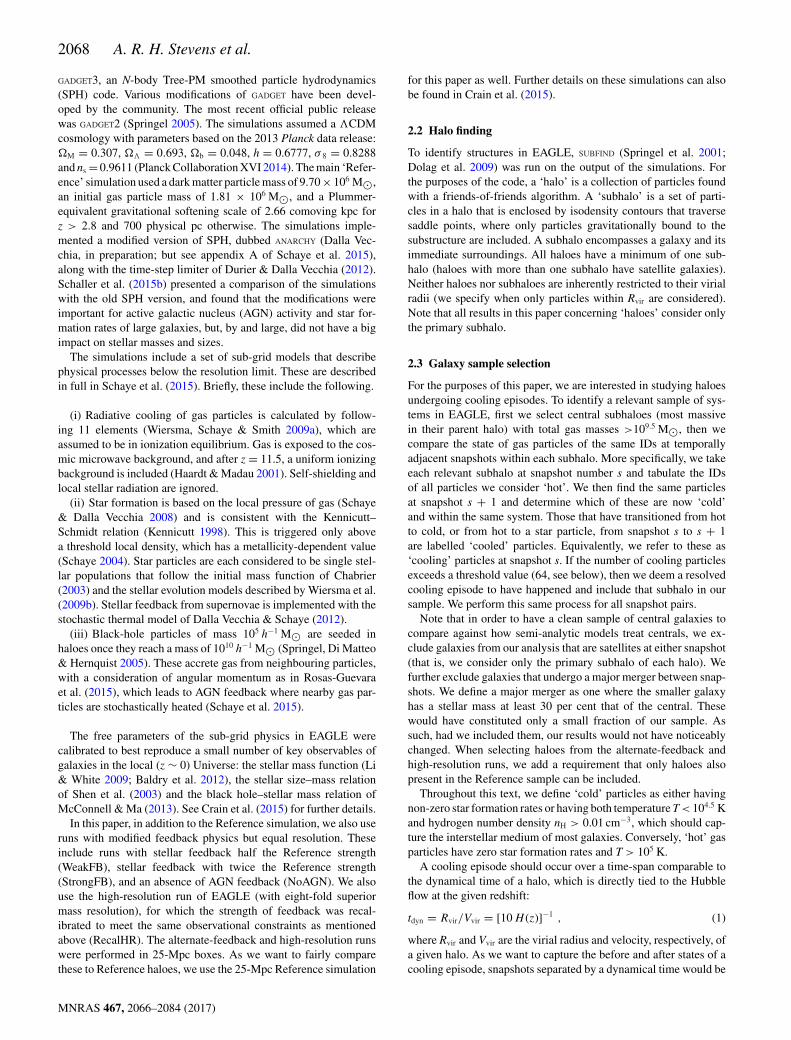
Figure 7. Metal fraction profiles for hot gas in our EAGLE haloes at z < 0.6,normalized by the average metal fraction in each case. The thick curvesgive the median for each labelled simulation. The shaded region covers the16th–84th percentile range for the Reference simulation, while the thincurves cover the same range for the WeakFB and StrongFB runs. Stellarfeedback is seen to enrich the centres of hot haloes with metals.
be strictly a function of redshift and cannot meaningfully find asecondary dependence on any integrated halo property (that a semi-analytic model would have access to).
3.3 Metallicity profiles of hot gas
Another common approximation made in analytic models is thatthe metallicity of hot gas is uniform throughout the halo. In reality,we would expect hot gas at the centre of haloes to be more metal-rich than at the outskirts, as the stars at the bottom of the potentialwell are what produce new metals. To demonstrate the degree towhich this is true for EAGLE, we calculate the mass-weightedmean metal fraction of particles in each spherical shell (as definedin Section 3.1) of each halo, and plot the normalized metal fractionprofiles of our sample haloes at z < 0.6 in Fig. 7. We include themedian and 16th–84th percentile range for the Reference, WeakFBand StrongFB simulations. At higher redshift, the behaviour ofthese three simulations is similar to the Reference case presentedat low redshift, and thus these have been omitted for simplicity.The RecalHR simulation is also consistent with the Reference casepresented here, and is omitted for clarity. In all cases, we findthat metallicity becomes increasingly variant towards the centresof haloes, with a general trend of metallicity increasing. The effectof stellar feedback enriching the hot halo is clear; by z < 0.6,the centres of haloes in the StrongFB simulation have the steepestgradients, and the WeakFB simulation the shallowest. As the rate atwhich gas cools is dependent on metallicity, metallicity gradientscan have an impact on the cooling calculation in a semi-analyticmodel, which we turn our attention to next.
3.4 Cooling time profiles
The primary purpose of semi-analytic models including prescrip-tions for the hot-gas density profile, temperature and metallicity isto determine a cooling rate at each time-step. It is, therefore, ofinterest what consequences will arise for the cooling rates from thedifferences in the profiles of the EAGLE haloes versus analytic ap-proximations. To investigate this, we must first address the typicalprocess for calculating cooling rates in semi-analytic models.
The majority of semi-analytic models (e.g. Cole et al. 2000;Hatton et al. 2003; Cora 2006; Croton et al. 2006, 2016; Somervilleet al. 2008b; Guo et al. 2011; Lee & Yi 2013) calculate coolingrates using some variation of the method presented in White &Frenk (1991), which is as follows (but see e.g. Monaco, Fontanot& Taffoni 2007 for a more detailed treatment). Given a spherically
symmetric distribution of hot gas, the ‘cooling time’ for hot gas ata given radius is first defined as
tcool(R) ≡ 3
2
Thot(R)
ρhot(R)
μmp kB
�(Thot(R), Zhot(R)), (7)
where �(T, Z) is the cooling function, commonly drawn from thetables of Sutherland & Dopita (1993), dependent on the temperatureand metallicity of the gas. One then defines the ‘cooling radius’,Rcool, as the radius at which the cooling time equals a relevant time-scale. For the purposes of this paper, we have chosen to equate thistime-scale to the dynamical time, in line with the SAGE family ofmodels (Croton et al. 2016; Stevens et al. 2016; Tonini et al. 2016),but this could have been informed by the free-fall time-scale instead,as in GALFORM, for example. The general argument then is that thecooling mass that crosses Rcool is approximately equal to the cold-gas mass deposition rate on to the galaxy (Bertschinger 1989). Fromthis continuity law, one can calculate the rate at which gas cools onto the galaxy as
mcool,model = 4π ρhot(Rcool) R2cool
(dtcool
dR
∣∣∣∣R→Rcool
)−1
. (8)
In the case where Rcool > Rvir, haloes are assumed to be in a cold-accretion regime in a semi-analytic model, where the cooling rate isthen taken as the ratio of the hot mass to the dynamical (or free-fall)time. We remind the reader that our EAGLE haloes are selected tobe in the hot mode of accretion.
Our intent here is not to compare the true cooling rates of EAGLEhaloes to those inferred by equation (8). To make that comparisonwould require a complete deconstruction of how feedback influ-ences cooling in both EAGLE and semi-analytic models. This isnon-trivial, as the way in which feedback and cooling are handledin semi-analytic models is not directly comparable to what goeson in a hydrodynamic simulation, and there is plenty of variationamongst models as well (see Lu et al. 2011). A model can havedegeneracies when it comes to cooling and heating rates, wherethe free parameters governing these are only really constrained ina relative sense, such that the net growth of (sometimes just thestellar content of) galaxies is representative of the observed Uni-verse. This is why many semi-analytic–hydrodynamic comparisonprojects have excluded feedback (and sometimes even star forma-tion) from the simulations entirely (e.g. Benson et al. 2001; Yoshidaet al. 2002; Helly et al. 2003; Cattaneo et al. 2007; Viola et al. 2008;Saro et al. 2010; Lu et al. 2011; Monaco et al. 2014). What we aimto address here is how the cooling time profiles, through equation(7), vary when we include the detail of the density, temperature andmetallicity profiles available to us from EAGLE. In Section 3.5,we go one step further, and calculate how the tcool(R) profiles ofour EAGLE haloes would translate into an effective semi-analyticcooling rate.
It is normal for the purposes of a semi-analytic model to simplifyequation (7) by taking Tvir as the temperature for all hot gas in thehalo, and assuming all hot gas to have the same metallicity. This thenleaves tcool(R) for a given halo dependent on the assumed densityprofile. We address the impact of the density profile on tcool(R) inFig. 8. The long-dashed and dot–dashed curves give the mediantcool(R) profiles after using analytic profiles of a singular isothermalsphere and β profiles with cβ = 0.1 and cβ (z) from equation (6),respectively. These profiles differ little, where the β fit makes anotable difference only for R � 0.3Rvir (especially at low redshift),where it is generally true that tcool < tdyn. As a result, the coolingradii calculated from these density profiles are all consistent. This is
MNRAS 467, 2066–2084 (2017)

2074 A. R. H. Stevens et al.
Figure 8. Cooling time of hot gas in our EAGLE halo sample, normalized by their respective dynamical times, as a function of radius, normalized by theirvirial radii. We present median profiles calculated from the EAGLE haloes through equation (7) in cases where we consider (i) only the density profiles ofthe halo with Thot(R) = Tvir and Zhot(R) = Zhot (dotted curves); (ii) both the density and temperature profiles with Zhot(R) = Zhot (short-dashed curves); and(iii) the density, temperature and metallicity profiles of the haloes (solid curves). In the latter case, we show the 16th–84th percentile range with the shadedregion. Included for comparison are the median cooling time profiles when assuming that the density profile follows (i) a singular isothermal sphere, (ii) a β
profile with constant cβ = 0.1, and (iii) a β profile with cβ calculated from equation (6), which takes Thot(R) = Tvir and Zhot(R) = Zhot in all three cases (seethe legend in the right-hand panel). The horizontal lines cover the inner 68 per cent of Rcool/Rvir values in each case, with matching linestyles. The verticalmarks through these give the median cooling radii. Complete information on the density, temperature and/or metallicity profiles of hot haloes leads to a greaterrange of cooling profiles than analytic approximations would give, which can impact cooling radii, thereby affecting the cooling rates one would calculate in asemi-analytic model.
shown by the horizontal lines in Fig. 8, which cover the 16th–84thpercentile range for Rcool/Rvir in each case, with the intersectingvertical marks giving the medians.
As a direct comparison to the analytic profiles, we calculatetcool(R) using the actual density profiles from each ReferenceEAGLE halo, while maintaining the use of Thot(R) = Tvir andZhot(R) = Zhot. The median profile (dotted curves in Fig. 8) isconsistent with the analytic cases in the outer parts of the halo, butdiverges for R � 0.4Rvir for all z < 4 (the scatter in all these cases isconsistent, but this is not shown for clarity). As a result, the coolingradii are systematically lower than their analytic counterparts. Thishighlights the fact that, even when using a density profile that fitsthe general population by construction, it is difficult to recover thetrue cooling radii of haloes from a hydrodynamic simulation.
Next, we consider the role of the temperature profiles of theEAGLE haloes on tcool(R). We again solve equation (7) withZhot(R) = Zhot, but use the actual profiles of the haloes for Thot(R)and ρhot(R). The median tcool(R) profile in this case is given bythe short-dashed curves in Fig. 8. Comparing this to the dottedcurves, we see that the profile flattens, which leads to a muchbroader range in cooling radii for the haloes. Even though a typicalEAGLE halo will have a radial variation in its temperature of nomore than a factor of ∼3 (cf. Fig. 3), this temperature structure cansignificantly impact the tcool(R) profile one infers for a halo, andtherefore would impact the cooling rate one would determine ina semi-analytic model.
As a final step, we include the metallicity profiles of the EA-GLE haloes and recalculate tcool(R). We include the median relationwith the solid curves, and the 16th–84th percentile range with theshaded region in each panel of Fig. 8. The addition of the Zhot(R)profile restores sensible cooling radius values that are consistentwith the haloes being in the hot mode of accretion. For complete-ness then, a model of halo gas that includes temperature structureshould also include metallicity structure for the sake of calculat-ing cooling radii and rates. For z > 0.6, these cooling radii are inmoderate agreement with the purely analytic profiles. The tcool(R)profiles flatten at low redshift, which leads to a broad range in cool-ing radii, which become systematically less than the cases of theanalytic profiles.
3.5 Model-equivalent cooling rates
In an ideal world, one would know the unique density, temperatureand metallicity profile of hot gas in every halo processed through asemi-analytic model. By using the measured profiles from EAGLE,we can solve equation (8) numerically for each halo, thereby deter-mining the ‘semi-analytic equivalent’ for the cooling rate with idealinformation. This can be compared against a more realistic calcu-lation for a semi-analytic model, where in addition to an analyticdensity profile, it is assumed that Thot(R) = Tvir and Zhot(R) = Zhot
for each halo. The results of Section 3.4 suggest that any of a singu-lar isothermal sphere, a β profile with cβ = 0.1 or a β profile withcβ (z) from equation (6) will work practically the same for calcu-lating a cooling rate. In the left-hand panel of Fig. 9, we comparethe cooling rates calculated by equation (8) using the full EAGLEprofile information against the case of an assumed singular isother-mal sphere (we have checked that this is essentially the same forthe case of a β profile).
The spread in the true Rcool values for the EAGLE haloes isgreater than that of the analytic models, as seen in all panels ofFig. 8. This then gives rise to the notable spread in the relativecooling rates seen in the left-hand (and middle) panel of Fig. 9. Inthe lower-redshift bins, the model Rcool values are systematicallytoo large, most clearly seen in the right-hand panel of Fig. 8. Thisthen translates into systematically higher cooling rates, as seen bythe evolution in the distributions of the left-hand (and middle) panelof Fig. 9.
Note that the cooling rates calculated by equation (8) do not con-sider feedback (of any kind), and hence are gross cooling rates (asopposed to net cooling rates – see below). If feedback were to affectthe density or temperature profiles of the hot gas in haloes signifi-cantly, then we might expect this feedback to still cause differencesin the gross cooling rates. While we showed that feedback does alterthe temperature at the centre of EAGLE haloes in Fig. 4, this is lessthan a factor of 2. Because the hot-gas density profiles also do notchange significantly when the strength of feedback is varied, thegross cooling rates calculated by equation (8) should agree for theReference and alternate-feedback simulations. To demonstrate oneexample, we compare mcool for the NoAGN simulation, as we did
MNRAS 467, 2066–2084 (2017)

How to get cool in the heat 2075
Figure 9. Normalized histograms for the relative analytic cooling rates calculated for model density profiles of hot gas versus those using the actual density,temperature and metallicity profiles from our sample of Reference and NoAGN EAGLE haloes, as labelled. The left-hand panel and middle panel compare grosscooling rates (equation 8), while the right-hand panel compares net cooling rates (equation 10). If the analytic approximations were sufficient for calculatingcooling rates, the distributions would be δ functions at the vertical dashed line.
for the Reference simulation, in the middle panel of Fig. 9. Whilethere are small differences compared with the left-hand panel, theevolution of the distributions and their peaks are in agreement. Re-sults for WeakFB and StrongFB are indeed similar, so we omit themfor simplicity.
While stellar feedback is often considered independently of cal-culating cooling rates in semi-analytic models (but not always – see,e.g. Monaco et al. 2007), radio-mode AGN feedback is generallyimplemented by directly suppressing the cooling rates calculatedthrough equation (8) (see Bower et al. 2006; Croton et al. 2006).Galaxies hosting a larger supermassive black hole will typicallyhave their cooling suppressed more. At later times, the haloes in oursample are bigger (see Fig. 2) and host heavier black holes. Becausethe suppressive heating from AGN need not be tied directly to thegross cooling rates of haloes, ratios of net cooling rates as calcu-lated in semi-analytic models with different hot-gas radial profileswill not be the same as the ratio of gross cooling rates. They will, infact, be systematically smaller for systems with an AGN, effectivelycounteracting the redshift evolution of the gross cooling rate ratiospresented in the left-hand and middle panels of Fig. 9.
To demonstrate the impact AGN heating might have on coolingrates in a semi-analytic model, we use an example model of radio-mode heating to calculate effective net cooling rates for the haloes.We calculate the heating rate based on the energy released fromBondi–Hoyle accretion (Bondi 1952) of hot gas in the halo:
mheat,model = 15π
16
(μmp)2
�(Tvir, Zhot)Gc2 κη mBH (9)
(as implemented similarly in Croton et al. 2006; Somervilleet al. 2008b), where mBH is the black-hole mass,1 κ is a modelparameter used to control the strength of feedback and η is the ef-ficiency with which the inertial mass of the gas is released duringaccretion on to the black hole. Here, we assume typical values ofκ = η = 0.1. The net cooling rate of gas in a halo can then be foundas the difference between equations (8) and (9):
mnet,model = mcool,model − mheat,model. (10)
1 A total of 94 per cent of the (sub)haloes in our sample have more than oneblack-hole particle. In a semi-analytic model, galaxies typically are onlyallowed one black hole; when a merger brings in a new black hole, it isassumed to merge immediately with any preexisting black hole. To mimicthis, we sum the masses of all black holes in an EAGLE galaxy to give mBH
to calculate mheat,model.
We calculate mnet for our haloes in the Reference simulation, usingthe true and analytic (singular isothermal sphere and β) radial pro-files. In the right-hand panel of Fig. 9, we present the ratio of themodel-equivalent net cooling rates using the EAGLE radial profiles(density, temperature and metallicity) to the singular isothermalsphere profile. Not only is the evolution of the distributions mini-mized compared to the ratio of gross cooling rates, but the widthsof the distributions are also greatly reduced. The latter would notbe true if the central temperature and metallicity of the hot haloeswere used in the Bondi–Hoyle model, however.
In conclusion, while the structural properties of hot gas in haloescan significantly affect gross cooling rates in semi-analytic models,the application of radio-mode feedback can compensate for most ofthis.
4 A N G U L A R M O M E N T U M O F C O O L I N G G A S
4.1 Conservation of angular momentum during cooling
An important aspect of most models of gas cooling is the assump-tion that the angular momentum of the gas is conserved. Of course,cooling gas can exchange angular momentum with many other partsof the halo in principle, especially through collisions with gas parti-cles not involved in cooling (including those already cold). Early at-tempts at forming spiral galaxies with cosmological, hydrodynamicsimulations were plagued by an ‘angular-momentum catastrophe’,where gas cooled too quickly and lost too much angular momen-tum (see e.g. Katz & Gunn 1991; Navarro & Benz 1991; Navarro& Steinmetz 1997, 2000). Solutions to this problem were found inbetter resolution (Governato et al. 2004) and more efficient subgridfeedback (e.g. Brook et al. 2011, 2012). With these improvements,we are now in a position to use a simulation like EAGLE to makepredictions about the angular-momentum conservation of coolinggas, or lack thereof, which is informative for analytic models of gascooling.
We measure the specific angular momentum, j, of cooling andcooled particles (i.e. immediately before and after cooling) in ourEAGLE haloes along their respective cooling particles’ axes of rota-tion on an individual basis and for the summed quantity of all coolingparticles involved in a single episode. The relative change in j foreach case is presented in the upper and middle panels of Fig. 10, re-spectively. These two cases allow us to distinguish between ‘strong’and ‘weak’ angular-momentum conservation (Fall 2002). In the‘strong’ case, individual particles would conserve j, whereas onlythe net j of a collection of particles needs to be conserved in the‘weak’ case. We bin our systems by redshift, as in the previous
MNRAS 467, 2066–2084 (2017)
2076 A. R. H. Stevens et al.
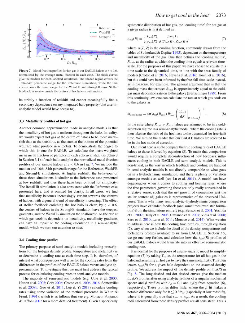
Figure 10. Relative change in the specific angular momentum component parallel to the rotation axis of cooling particles during cooling episodes, comparedto the initial state. The left-hand panels include haloes from our Reference EAGLE sample, while the right-hand panels include those from the RecalHR run.The top panels consider particles individually. The middle and bottom panels consider the change in net specific angular momentum of all cooling particles ina single episode, i.e. on a halo-by-halo basis. Where the top two rows of panels bin by redshift, the bottom row of panels bins by the λR value of the centralgalaxy for all z < 1.7. The short, vertical marks give the mean of each distribution for respective linestyles. If angular momentum were always conserved alongthe cooling axis, the distributions would be δ functions matching the vertical, dashed line. Instead, we see angular momentum losses in the cooling gas. Weperform Kolmogorov–Smirnov tests to compare the consistency of the halo distributions between 4 > z > 1.7 and z < 0.6, and between the distributions forλR ≤ 0.25 and λR > 0.75. The D-value printed in the panels gives the maximum vertical separation of the cumulative probability distributions, while thep-value is the probability that the means of the distributions would be as separated as they are under the pretext that they come from the same underlyingpopulation. A little less angular momentum appears to be lost when gas cools on to a rotationally supported galaxy.
sections, and show distributions for the relative change in angularmomentum for each of these bins. Because resolution is knownto play a role in j losses, we present both the Reference andRecalHR simulations in the left-hand and right-hand panels ofFig. 10, respectively.
It is clear from the top panels of Fig. 10 that individual particlesdo not conserve angular momentum while cooling, and thus EAGLEhaloes do not demonstrate strong j conservation. Comparing this tothe middle panels, those particles appear to be exchanging some oftheir angular momentum between one another, as the net change in jfor the collection of particles provides a narrower distribution with apeak closer to zero. Yet, in both cases, the means of the distributionsare negative. Therefore, on average, angular momentum is lost bygas as it cools on to EAGLE galaxies; i.e. even weak j conservationis not satisfied. There is no clear evolution in the distributions foreither the upper or middle panels of Fig. 10 for the Reference simu-lation; for the highest- to lowest-redshift bins, the average net loss ofj during a cooling episode is approximately 55, 64 and 57 per cent,respectively. The highest- and lowest-redshift histograms are alsoconsistent according to the Kolmogorov–Smirnov test (see Fig. 10).We find that at a higher resolution (the RecalHR run), j losses dur-ing cooling are reduced at higher redshift, on average. We suggestthat, by itself, this is not enough to claim any generic correlationbetween �j/ji and z, especially as the results between simulationsagree at low redshift. We come back to this point in Section 4.2.
Galactic discs in EAGLE are known to be realistic in their size(Schaye et al. 2015; Lange et al. 2016; Furlong et al. 2017). Yet,the gas that cools loses a fraction of angular momentum that isconsistent with the large percentages reported when the ‘angular-momentum catastrophe’ produced simulated discs that were tooconcentrated (cf. Katz & Gunn 1991). While, indeed, too muchabsolute angular momentum was lost during cooling in early hydro-
dynamic, cosmological simulations, evidently the correct amountof specific angular momentum was lost, based on our results.
The frequency of particle interactions and collisions will deter-mine the potential for angular-momentum loss of cooling particles.We hypothesize that in a rotationally supported system, where thereis less random motion, collisions might be fewer, and thus less an-gular momentum might be lost. To test this, we first quantify therelative level of rotation and dispersion support in our galaxies us-ing the λR parameter, introduced by Emsellem et al. (2007). Galax-ies with λR ∼ 0 are predominantly dispersion-supported, whereasthose with λR ∼ 1 are predominantly rotationally supported. For ourEAGLE galaxies, we measure the property as
λR =∑
∗ m∗ jz,∗∑∗ m∗
√j 2z,∗ + r2∗ v2
z,∗, (11)
where the sums are over all star particles associated with the mainsubhalo within the ‘BaryMP’ galactic radius defined by Stevenset al. (2014, where the cumulative mass profile of the stars andcold gas reaches a constant gradient), and jz and vz are the specificangular momentum and velocity components along the galaxy’srotation axis, respectively, as measured in the galaxy’s centre-of-momentum frame.2 In the bottom panels of Fig. 10, we again showthe relative net loss of specific angular momentum during coolingevents, but now bin galaxies by λR, including all systems for z < 1.7.By excluding those in the range 1.7 < z < 4, we eliminate thepopulation of high-z systems from RecalHR that we have shown
2 Note that this calculation for λR does not include the intricacies required tocompare against observations as in Naab et al. (2014), as we simply require arelative measure of this quantity for internally comparing EAGLE galaxies.
MNRAS 467, 2066–2084 (2017)

How to get cool in the heat 2077
Figure 11. Probability distributions for the ratio of the magnitudes of net specific angular momentum of cooling gas to that of the halo, drawn from our sampleof Reference and RecalHR EAGLE systems. The top panels cover all systems in each redshift bin, while the bottom panels cover all z < 1.7 and bins by λR ofthe central galaxy. The dashed, vertical line indicates where jcooling = jhalo, which is often assumed in galaxy formation models. The short, vertical marks givethe means of the distributions. We perform Kolmogorov–Smirnov tests on the consistency of the distributions in each panel, and note the cases where there ispotential inconsistency (see caption of Fig. 10). Cooling gas carries more specific angular momentum than the halo on almost all occasions.
lose less j during cooling. We would have otherwise had biasedresults, as the average λR of the galaxies is lower at higher z.
For the Reference and RecalHR simulations, we find a weaktendency for j losses to be reduced for high-λR systems. To quantifythis statistically, we have compared the distributions for the highestand lowest λR histograms in the bottom panels of Fig. 10 usingthe Kolmogorov–Smirnov test, the results of which are given inthe panels. The low p-values (10−9.4 and 10−4.4 for the Referenceand RecalHR simulations, respectively) suggest that there is a non-negligible statistical significance to the separation of the meansof the distributions, although this is less significant for the higherresolution simulation. We thus tentatively find these results in favourof our hypothesis. Our results suggest that any reduction in j lossesduring cooling caused by stronger rotation in the central galaxy is,at most, a few tens of per cent.
4.2 Relative orientation and magnitude of specific angularmomenta
As already discussed, galaxy formation models typically assumethat the net specific angular momentum of hot gas about to cool,j cooling, is equivalent to that of all the hot gas in the halo, jhot, andto that of the entire halo itself, jhalo, both in terms of magnitudeand direction. Without the ability to directly measure the motion ofdark matter in haloes to independently measure a halo’s spin, it isimpossible to determine if j cooling and jhalo are the same empiricallywith observational methods. Simulations are the only current meansof addressing this in any capacity. Previous studies of cosmological,hydrodynamic simulations have shown that gas and dark matter inhaloes tend to have different and/or offset specific angular momenta(e.g. van den Bosch et al. 2002; Chen, Jing & Yoshikaw 2003; vanden Bosch, Abel & Hernquist 2003; Sharma & Steinmetz 2005;Sharma, Steinmetz & Bland-Hawthorn 2012). Attention has notbeen given specifically to the cooling particles before, however.
4.2.1 Magnitude
We directly measure the ratio jcooling/jhalo from our EAGLE haloes,and present distributions for this ratio for bins of redshift in the toppanels of Fig. 11. We see that cooling gas typically has more specificangular momentum than the halo. This result is contrasting (butnot opposing) to the combined results of observations and models
that suggest the stellar content of galaxies typically has a lowerspecific angular momentum than their haloes (e.g. Romanowsky &Fall 2012; Stevens et al. 2016). As discussed in Section 4.1, someof this angular momentum is lost during the cooling process. Asseen in the top panels of Fig. 11, there is no clear evolution injcooling/jhalo for our EAGLE haloes. We do, however, find the meanratio to be lower for RecalHR at higher redshift, which appears tobe statistically significant, based on a Kolmogorov–Smirnov test(see the top right-hand panel of Fig. 11). This is balanced by thefact that less angular momentum is lost during the cooling processfor these specific haloes, as shown in Section 4.1. If we comparethese findings with the lower left-hand panel of Fig. 3, we seethat the temperature of the cooling gas in these haloes is lower atthe ‘beginning’ of the cooling episode for the RecalHR run. Theevidence suggests that the population of RecalHR haloes in oursample for 4 > z > 1.7 effectively had a head start in coolingover the same haloes in the Reference simulation, and thus weremeasured at a moment when the gas was already cooler and hadalready lost some of its specific angular momentum. This wouldimply that the angular-momentum measurements in the Referenceand RecalHR runs are entirely consistent.
We have already shown tentative evidence that gas cooling on to arotationally supported galaxy in EAGLE loses less specific angularmomentum than that cooling on to a dispersion-supported galaxy(Fig. 10). In the bottom panels of Fig. 11 we also break jcooling/jhalo
into bins of λR. There is a population of low-λR galaxies, in boththe Reference and RecalHR simulations, that show high values forjcooling/jhalo, but are not abnormal in any other respect we can find.We find that nearly all the excess specific angular momentum is lostduring cooling for these systems. Modulo those few systems, thedistributions for jcooling/jhalo for various λR are entirely consistentwith each other. In other words, gas should not be aware of whattype of galaxy it will cool on to at the moment it begins to cool,which appears to indeed be the case for EAGLE.
It is not just the cooling gas whose j exceeds that of thehalo. In fact, hot gas in general has preferentially high j in ourEAGLE haloes, as shown in Fig. 12. This result is consistent withprevious studies of non-radiative hydrodynamic simulations (Chenet al. 2003; Sharma & Steinmetz 2005), but contends with the earlierwork of van den Bosch et al. (2002). The fact that 〈jhot/jhalo〉 > 1automatically explains why 〈jcooling/jhalo〉 > 1. Yet, we also find that
MNRAS 467, 2066–2084 (2017)

2078 A. R. H. Stevens et al.
Figure 12. Normalized histograms of the ratio of the magnitudes of netspecific angular momentum of hot gas to that of the entire halo (within Rvir)for our Reference (top panel) and RecalHR (bottom panel) EAGLE systemsfor three redshift bins. The vertical, dashed line indicates where jhot = jhalo.The short, vertical marks are the means for each distribution. Hot gas inhaloes has a preferentially higher specific angular momentum than the haloas a whole.
Figure 13. Normalized histograms of the ratio of the magnitudes of netspecific angular momentum of cooling gas to that of hot gas for our ReferenceEAGLE systems. In all panels, jhot is calculated using only the particleswithin the virial radius. The top panel calculates jcooling using all coolingparticles. The middle panel considers only cooling particles within the virialradius. The bottom panel presents the jcooling component for particles withinthe virial radius projected on to the axis of rotation of the hot particles. Thevertical, dashed line indicates where jcooling = jhot. The short, vertical marksare the means for each distribution.
〈jcooling/jhot〉 > 1 for our haloes. This can be seen by comparingFigs 11 and 12 and is shown more explicitly in the top panel ofFig. 13. A contributing factor to this is that jhot has been measuredexclusively for hot particles within Rvir, while jcooling considers allcooling particles here. Once the virial-radius restriction is imposedon jcooling too, the highest j particles are eliminated, and so thisbecomes more consistent with jhot, as seen in the middle panel ofFig. 13. Still, when we average over our full halo sample at allredshifts, we find 〈jcooling(<Rvir)/jhalo〉 � 1.4. Most of this extra
jcooling comes from a non-zero component orthogonal to jhot. Thisis demonstrated by the bottom panel of Fig. 13, which now projectsj cooling on to jhot. Here, the projected magnitude of jcooling is con-sistent with jhot, once averaged over all redshifts.
If one assumes that gas particles at the centre of the halo havelower j than those at the outskirts, then our result from Fig. 5(that cooling gas originates preferentially from the halo centre,regardless of the underlying hot-gas distribution, while the hot gasforms a core) can explain why there is an evolutionary decline injcooling/jhot, seen in all panels of Fig. 13. We remind the reader thatbecause we looked for particles that transitioned from hot to coldover time-steps of several hundred Myr, we will have missed anyparticles that both cooled and were reheated over that time. Whilewe suggested in Section 2.3 that the fraction of these particles isgenerally small, the lowest j particles are preferentially reheatedby feedback (see Brook et al. 2011, 2012), so our jcooling valuesare more like close upper limits. Thankfully, jhot is not subject tothis bias, so our finding that gas has specific angular momentum inexcess of jhalo when it begins to cool in EAGLE haloes is robust.
4.2.2 Orientation
The direction of the angular momentum of the cooling gas is alsoimportant for how the new material will alter the disc. In the toppanels of Fig. 14, we show the angular offsets of the spin vectors ofhot gas about to cool and hot gas in general for our EAGLE haloes.Regardless of redshift, these are typically offset by tens of degrees.The second row of panels in Fig. 14 shows the angular differencein rotation axis of the cooling and cooled particles, that is, beforeand after the transition from hot to cold. Again, differences of tensof degrees are common, indicating that gas particles precess duringcooling. In fact, they precess to come in line with the preexistingcold gas in the galaxy, as seen by the small angular differences inthe rotation axes of the cooled and cold particles in the third row ofpanels in Fig. 14. A combination of the cooling gas’s rotation axisbeing consistently offset from the hot gas as a whole with the gasbeing subject to precession sets up an offset between the rotationaxes of the cold gas in the galaxy and its hot halo. This is shown bythe bottom panels of Fig. 14, where, once again, offsets of many tensof degrees are common and persist to z = 0. Having such an offsetcan lead to warped discs (Roskar et al. 2010). As with our otherresults, we do not find a clear, systematic difference between theReference (left-hand panels of Fig. 14) and RecalHR (right-handpanels) runs, suggesting that this is indeed a physical result.
Because most cooling occurs in the inner part of the hot halo(Fig. 5), one might also expect the inner hot halo’s rotation axis tobe better aligned with the cooling gas. We calculate whether therotation axis offset between cooling and hot gas varies when onlyhot gas internal to a given radius is included, which we present inFig. 15. Contrary to expectation, we find that the inner hot gas istypically less aligned with the cooling gas. Any evolution in theprofiles in Fig. 15 is minimal for our sample of EAGLE haloes, asseen by the similarity of the curves in Fig. 15. The Reference (upperpanel) and RecalHR (lower panel) simulations again produce thesame result, so we can trust that this is not predominantly an effectof resolution. Our result is contrasting (but not at all opposing) tothe results of Zavala et al. (2016), who find that the evolution of jof stars in EAGLE galaxies is more closely tied to that of the innerdark matter halo (<0.1Rvir), rather than the halo in its entirety.
The relative orientations and magnitudes of j for various particletypes in haloes in general are an interesting topic, which we areinvestigating in detail in an accompanying paper (Contreras et al., in
MNRAS 467, 2066–2084 (2017)

How to get cool in the heat 2079
Figure 14. Angular separations between rotation axes of gas particle groups during cooling. The top panels give the difference between all the hot particlesand those about to cool. The second row of panels is the change in the rotation axis of the particles that cool over the cooling episode. The third row of panelsare for all cold gas and the particles that have just cooled. The bottom panels compare the rotation axes of all cold gas to all hot gas. Cooling gas need not bealigned with the rest of the hot gas in the halo, and it precesses during the cooling process to become aligned with gas that is already cold.
Figure 15. Angular separation between spin directions of hot gas in haloeswithin a given radius and all cooling gas for the same haloes. Cooling gas ispoorly aligned with hot gas on all scales, regardless of redshift or resolution.
preparation). The sample of cooling systems used here is consistentwith the differences in direction and magnitude of j between baryonsand dark matter in all EAGLE haloes to be presented there. Thatpaper will address uncertainties in angular momentum as a functionof the number of particles used; in general, �100 particles arerequired for trustworthy measurements of individual haloes. We donot find any significant changes to our conclusions here (that areconcerned with the population) if we exclude haloes with <100particles though.
5 A F T E R C O O L I N G : C O L D G A S IN G A L A X I E S
5.1 Radial surface density profiles of gas discs
In the picture of disc formation proposed by Fall & Efstathiou(1980), gas cools and collapses to form an exponential disc while
conserving angular momentum:
cooled(r) = 0e−r/rd � mcooled
2πr2d
e−r/rd , (12)
where rd � Rvir is the scale radius of the disc. The exponential-ity of discs is a typical assumption of galaxy formation models,where some even maintain that a disc must always be exponential(e.g. Cole et al. 2000; Hatton et al. 2003; Croton et al. 2006, 2016;Somerville et al. 2008a; Guo et al. 2011). But only relatively re-cently have resolved observations of the H I and CO (H2) distributionin local spiral galaxies been made (e.g. Walter et al. 2008; Leroyet al. 2009), allowing us to actually see what they are like. The 33galaxies analysed by Bigiel & Blitz (2012) suggest that while anexponential profile broadly describes the average galaxy at inter-mediate radii, there is plenty of deviation from exponentials, anda strong suggestion of cusps existing at the centres of these discs.With EAGLE, we can not only check the exponentiality of gas discs,but also compare directly to equation (12).
We present surface density profiles for recently cooled and allcold gas of our sample of EAGLE haloes in Fig. 16 (top and bottompanels, respectively). To build these profiles, we find the rotationaxis of the cold (cooled) particles to determine the plane of thegalaxy (freshly cooled gas), and measure the surface density inannuli3 in this plane. Consistent with our measurements of the hotgas profiles, the widths of the annuli are adapted to contain the samenumber of particles, while respecting the softening scale. A totalof 100 annuli are used for the cold gas, and 20 are used for thecooled gas. We then fit an exponential to each profile and normalizethe annuli’s radii by the fitted scalelength. By normalizing the sur-face densities as well, we are able to see how well an exponential
3 For our intents and purposes, an annulus is a cylindrical shell that cannotexceed the virial sphere in height.
MNRAS 467, 2066–2084 (2017)

2080 A. R. H. Stevens et al.
Figure 16. Surface density profiles for cold gas particles in our sample of EAGLE galaxies. As for previous figures, we present three redshift ranges for theReference and RecalHR simulations, presenting their median profiles (solid and short-dashed curves, respectively) and 16th–84th percentile ranges (shadedregions). Radial distances have been normalized for each galaxy by their fitted exponential scale radius, rd,fit. The top row of panels considers only therecently cooled particles, whereas the bottom panels consider all cold particles. All surface densities have been normalized by the amount of cooled/cold gasconsidered and the square of the scale radius. The long-dashed line is a precise exponential (equation 12). The dot–dashed curves give the median profile forthe rotation-dominated galaxies (λR > 0.75) for each subsample of the Reference haloes. With the addition of a central cusp, an exponential describes theprofile of recently cooled gas well, but only works as well for cold discs as a whole at low redshift.
describes the entire galaxy population as a whole. Note that rd,fit is adifferent quantity for the cooled(r) and cold(r) profiles in Fig. 16.
The top panels of Fig. 16 show that cooled(r) for EAGLE galaxiesis nicely centred on equation (12), with a scatter increasing at lowerredshift (the 68 per cent confidence range is 0.53, 0.62 and 0.79 dextall on average for the highest- to lowest-redshift bins, respectively).The profiles include a cusp, seen at r � 0.6rd for the highest-redshiftbin, with the prominence of this feature growing modestly down toz = 0. Approximately 20 per cent of the cooled gas mass lies insider < 0.6rd when averaged over all galaxies in our sample for eitherthe Reference or the RecalHR simulation. If these profiles wereexponential all the way to the centre, only 12 per cent of their massshould lie inside r < 0.6rd.
It is worth highlighting the fact that, because every EAGLE pro-file has been normalized by a fitted exponential scale radius, if anexponential were a general, genuine, good fit for the surface densityprofiles in Fig. 16, the EAGLE profiles should cluster about thelong-dashed line with a small amount of scatter. A cusp can stillbe recovered from an otherwise exponential profile, provided thenumber of points being fitted to in each cusp is not a large fractionof those in the total profile. This is what is seen in the top panels.On the other hand, the bottom panels of Fig. 16 show that, at higherredshift, the cold(r) profiles are curved for the entire plotted range(cf. the long-dashed line). This implies that an exponential (evenwith a cusp) is too simplistic to describe these profiles in general.
Of course, the galaxies in our sample need not be all rotationallysupported, and hence may not have well-behaving, classical discs.To this point, we overplot the median surface density profiles forcold and recently cooled gas for the rotation-dominated galaxieswith λR > 0.75 in Fig. 16 with dot–dashed curves. By selectinggalaxies we expect to be more disc-like, we find no difference in thenormalized surface density profiles for cold or recently cooled gas.While the recently cooled gas in these galaxies lost marginally lessj during the cooling process (Fig. 10), this has not translated into adifference in cooled(r).
In a semi-analytic model, one must put in what the scalelength ofthe cooling disc is. If one assumes that gas cools into an exponentialdisc, that is, jcooled = jhalo, and that the disc has a flat rotation velocitywith vrot = Vvir, it is straightforward to show that the scaleradius ofthat exponential disc is
rd,model ≡ jhalo
2Vvir(13)
(e.g. Fall 1983; Mo et al. 1998). Equation (13) has formed the basisof determining (initial) disc sizes in many semi-analytic models(e.g. Hatton et al. 2003; Croton et al. 2006; Fu et al. 2010), but morecomplex algorithms are also popular (e.g. Cole et al. 2000).
We showed in Section 4 that the assumptions about the angularmomentum of the cooling gas required for equation (13) to be accu-rate do not agree with EAGLE, so we would expect some differencebetween the model scalelength, rd,model, and the fitted scalelength,rd,fit. After measuring the net specific angular momentum of eachhalo in our EAGLE sample as
jhalo = | ∑p mp rp × vp|∑p mp
(14)
(where subscript p is for particles of all types within Rvir), we canquantify how discrepant rd,model is from rd,fit.
In Fig. 17(a), we present normalized histograms for the ratio ofrd,fit/rd,model for both the Reference and RecalHR haloes, for allz < 4. Both simulations find an almost lognormal distribution forthis ratio, where it is almost always true that rd,fit > rd,model. Theidea that rd ∝ jhalo/Vvir (equation 13) came from the assumptionsthat jcooled = jhalo and that the cooled gas all rotated with velocityVvir. In practice, we should really expect rd ∝
∼jcooled/vrot, where vrot
is the mass-weighted mean tangential velocity of the cooled gas.This then gives
rd,fit
rd,model� jcooledVvir
jhalovrot. (15)
MNRAS 467, 2066–2084 (2017)
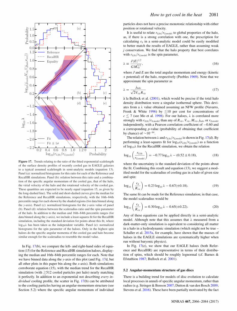
How to get cool in the heat 2081
Figure 17. Trends relating to the ratio of the fitted exponential scalelengthof the surface density profiles of recently cooled gas in EAGLE galaxiesto a typical assumed scalelength in semi-analytic models (equation 13).Panel (a): normalized histograms for this ratio for each of the Reference andRecalHR simulations. Panel (b): relation between this ratio and a combina-tion of the specific angular momentum of the cooled gas, that of the halo,the virial velocity of the halo and the rotational velocity of the cooled gas.These quantities are expected to be nearly equal (equation 15, as given bythe long-dashed line). The solid and short-dashed curves give the median forthe Reference and RecalHR simulations, respectively, with the 16th–84thpercentile range for each shown by the shaded regions (for data binned alongthe y-axis). Panel (c): normalized histograms for the y-axis value of panel(b). Panel (d): relation between the scaleradius ratio and the spin parameterof the halo. In addition to the median and 16th–84th percentile ranges (fordata binned along the y-axis), we include a least-squares fit for the RecalHRsimulation, including the standard deviation for points about this fit, wherelog10λ has been taken as the independent variable. Panel (e): normalizedhistograms for the spin parameter of the haloes. Only in the highest spinhaloes do the specific angular momenta of the cooled gas and halo becomesimilar enough for the scaleradius to resemble the model value.
In Fig. 17(b), we compare the left- and right-hand sides of equa-tion (15) for the Reference and RecalHR simulation haloes, display-ing the median and 16th–84th percentile ranges for each. Note thatwe have binned data along the y-axis of this plot (and Fig. 17d, butall other plots in this paper bin along the x-axis). Both simulationscorroborate equation (15), with the median trend for the RecalHRsimulation (with �512 cooled particles per halo) nearly matchingit perfectly. In addition to an exponential not describing every in-dividual cooling profile, the scatter in Fig. 17(b) can be attributedto the cooling particles having an angular-momentum structure (seeSection 5.2) where the specific angular momentum of individual
particles does not have a precise monotonic relationship with eitherposition or rotational velocity.
It is useful to relate rd,fit/rd,model to global properties of the halo,as, if there is a strong correlation with one, the prescription forcalculating rd in a semi-analytic model could be easily modifiedto better match the results of EAGLE, rather than assuming weakj conservation. We find that the halo property that best correlateswith rd,fit/rd,model is the spin parameter,
λ ≡ J |E|1/2
GM5/2vir
, (16)
where J and E are the total angular momentum and energy (kinetic+ potential) of the halo, respectively (Peebles 1969). Note that weapproximate the spin parameter as
λ = jhalo√2VvirRvir
(17)
a la Bullock et al. (2001), which would be precise if the total halodensity distribution were a singular isothermal sphere. This devi-ates from a λ value obtained assuming an NFW profile (Navarro,Frenk & White 1996) by �10 per cent for concentrations ofc � 7 (see Mo et al. 1998). For our haloes, λ is correlated morestrongly with rd,fit/rd,model than any of Rvir, Vvir, Mvir, jhalo or rd,model
independently, with a Pearson correlation coefficient of −0.60 anda corresponding p-value (probability of obtaining that coefficientby chance) of ∼10−84.
The relation between λ and rd,fit/rd,model is shown in Fig. 17(d). Byperforming a least-squares fit for log10(rd,fit/rd,model) as a functionof log10λ for the RecalHR simulation, we obtain the relation
log10
(rd,fit
rd,model
)= −0.77 log10 λ − (0.52 ± 0.18), (18)
where the uncertainty is the standard deviation of the points aboutthe fit. Combining this result and equation (13), we suggest a mod-ified model for the scaleradius of cooling gas in a halo of given sizeand spin:
log10
(rd
Rvir
)= 0.23 log10 λ − 0.67(±0.18). (19)
The same fit can be made for the Reference simulation; in that case,the model scaleradius would be
log10
(rd
Rvir
)= 0.30 log10 λ − 0.65(±0.22). (20)
Any of these equations can be applied directly in a semi-analyticmodel. Although note that this assumes that λ measured from adark-matter-only simulation is equivalent to considering all matterin a halo in a hydrodynamic simulation (which might not be true –Schaller et al. 2015a, for example, have shown that the masses ofhaloes in the EAGLE simulations are systematically higher whenrun without baryonic physics).
In Fig. 17(e), we show that our EAGLE haloes (both Refer-ence and RecalHR) are representative in terms of their distribu-tion of spins, which should be roughly lognormal (cf. Barnes &Efstathiou 1987; Bullock et al. 2001).
5.2 Angular-momentum structure of gas discs
There is a building trend for models of disc evolution to calculatelocal processes in annuli of specific angular momentum, rather thanradius (e.g. Stringer & Benson 2007; Dutton & van den Bosch 2009;Stevens et al. 2016). These have been partially motivated by the fact
MNRAS 467, 2066–2084 (2017)

2082 A. R. H. Stevens et al.
Figure 18. As for Fig. 16, but now presenting normalized surface density profiles for recently cooled (top panels) and all cold (bottom panels) gas as a functionof specific angular momentum. Because the axes are normalized by best exponential fits, if these profiles were generally well described by an exponential, weshould see a tight relation about the long-dashed line in each panel. Instead, we find that an exponential as a function of specific angular momentum is a lessaccurate description of the profiles to one as a function of radius (cf. Fig. 16).
that galaxies have dynamic and non-uniform velocity structures.One can rewrite equation (13) as an exponential function of specificangular momentum, thereby relaxing the requirement that coolinggas should settle with a constant rotational velocity:
cooled(j ) = 0(jd)e−j/jd (21)
(e.g. as implemented in the DARK SAGE semi-analytic model; Stevenset al. 2016). Here, we investigate the angular-momentum structureof the cooled and cold gas profiles of our EAGLE galaxies anddetermine whether equation (21) can approximate them.
We measure the mean j of particles in each annulus for whichwe have measured surface density values for our EAGLE galaxies.This gives us cooled(j) and cold(j) profiles, to which we fit equa-tion (21), then normalize these profiles based on the fitted jd. Theseare presented in Fig. 18. At intermediate to low redshifts, an expo-nential for cooled(j) describes the profiles reasonably well, but thisis not the case at a high redshift. For 1.7 > z > 0.6, there is lessof a featured cusp for cooled(j) than for cooled(r). This could beexplained by the rotational velocities (and hence specific angularmomenta) decreasing rapidly at the centres of discs, where pressuresupport becomes comparable to rotational support. In general, wefind that the scatter in the profiles is reduced when considering sur-face density as a function of radius instead (cf. Figs 16 and 18). Wefind that these conclusions extend to the overall cold gas profile,and that they apply to the general galaxy population (in our sam-ple) as well as the most rotationally supported systems (λR > 0.75,which should be the most discy – cf. solid and dot–dashed curvesin Fig. 18).
While our findings suggest that one would be better off usingequation (12) rather than (21) in a model of galaxy formation, ithas been shown that using the latter expression for cooling in asemi-analytic model with disc structure can successfully reproducethe properties of local galaxies, including the relation between thetotal mass and specific angular momentum of stellar discs (Stevenset al. 2016). Of course, disc instabilities and feedback will regulatethe structure of a galaxy (as a function of either specific angularmomentum and radius), so the manner in which gas cools does
not provide a complete picture by itself. An assessment of theimportance of details surrounding cooling versus internal regulatoryprocesses in accurately describing galaxy evolution with respect toobservations would serve as a useful follow-up study to this work.
6 SU M M A RY
We have studied the hot mode of accretion of gas on to galaxiesin the EAGLE simulations. As detailed in Section 2.3, we selectedsystems where a sufficient number of gas particles cooled betweensnapshots in order to learn about the state of haloes undergoingcooling and the galaxies they host. Our findings presented in thispaper can be summarized as follows.
(i) The temperature of hot gas in haloes is within a factor of 2of the virial temperature across all radii (Section 3.1). The gradi-ent of the temperature profiles steepens with time, due in part tostellar feedback. As centres become hotter, they become less dense,leading to shallower density gradients and the formation of a corein the hot gas (Section 3.2). The hot-gas density profiles are wellapproximated by a β profile. We have parametrized this as a simplefunction of redshift (equation 6), which can easily be adopted bysemi-analytic models.
(ii) Using the precise density, temperature and metallicity pro-files of hot gas in the EAGLE haloes leads to different (and morevaried) cooling time profiles from those one would obtain assuminga singular isothermal sphere or β profile for a halo with the sametotal mass content, net metallicity and virial temperature. At lowredshift, these profiles are shallower, leading to cooling radii thatare systematically smaller (and, again, more varied), which wouldtranslate into lower cooling rates under the model of White & Frenk(1991).
(iii) The density profiles of cooling gas remain nearly unchangedwith time, irrespective of the underlying hot gas (Section 3.1).While perhaps most alike an exponential, the density profilesof cooling gas are consistent with a singular isothermal sphere(Section 3.2). So long as models only require cooling gas to look
MNRAS 467, 2066–2084 (2017)

How to get cool in the heat 2083
like it is coming from an isothermal sphere, this seems to be areasonable approximation.
(iv) Outflows from AGN feedback appear to help regulate thetemperature profiles of cooling gas (Section 3.1). These becomelower and shallower in the centres of haloes over time in responseto the decrease in hot-gas density there, which minimizes the op-portunity for cooling.
(v) Over the course of cooling, gas loses approximately60 per cent of its specific angular momentum, on average(Section 4.1). This value is comparable to losses quoted duringreports of the ‘angular-momentum catastrophe’, yet the galaxies inEAGLE are far from catastrophic. We find a weak tendency for gascooling on to rotationally supported galaxies to lose a lesser fractionof its specific angular momentum.
(vi) Gas in the process of cooling typically begins with a specificangular momentum several times greater than that of the halo. Itsmagnitude is largely consistent with the hot gas as a whole, butthe spin direction is offset from the rest of the hot gas by tens ofdegrees (Section 4.2). Interestingly, the inner hot gas of the halois even less well aligned with the cooling gas, despite the coolinggas predominantly originating from the inner halo (cf. Sections 3.2and 4.2). As gas cools, it precesses to become well aligned with thepreexisting gas disc.
(vii) Recently cooled gas is well approximated by an exponentialsurface density profile as a function of radius (Section 5.1), with theexception of a central cusp, which contains ∼20 per cent of the totalcooled mass. In general, this is more precise than an exponentialas a function of specific angular momentum (Section 5.2). Becausethe cooled gas tends to have a higher specific angular momentumthan that of the halo, the best-fitting scaleradius for these surfacedensity profiles is typically larger than expected from the standardmodel of disc formation (Fall & Efstathiou 1980; Mo et al. 1998).This radius is still strongly tied to the spin parameter of a halo, forwhich we provide a new expression (cf. equations 19 and 20).
Our results suggest that some of the assumptions surroundingthe cooling of hot gas in (semi-)analytic galaxy formation modelsshould be revised. While the parameters of models are often tunedto match the properties of galaxies in the local Universe, by alteringthe prescriptions surrounding cooling, the star formation historiesand higher redshift properties of these galaxies will change. Thiscould, therefore, be fruitful in the quest for developing a model ofgalaxy evolution that can simultaneously explain the high-redshiftUniverse and low-redshift Universe.
AC K N OW L E D G E M E N T S
We thank the city of Perth for its record heat-wave in 2016 Februaryinspiring the title of this paper. We thank the referee for a construc-tive report, which led to several improvements in this paper.
This work was supported by a Research Collaboration Awardat the University of Western Australia. Parts of this research wereconducted by the Australian Research Council Centre of Excel-lence for All-sky Astrophysics (CAASTRO), through project num-ber CE110001020. SC acknowledges support from the CONICYTDoctoral Fellowship Programme.
We acknowledge the Virgo Consortium for making their sim-ulation data available. We thank PRACE for the access to theCurie facility in France. We have used the DiRAC system, whichis a part of the National E-Infrastructure at Durham University,operated by the Institute for Computational Cosmology on be-half of the STFC DiRAC HPC Facility (www.dirac.ac.uk); the
equipment was funded by BIS National E-infrastructure capitalgrant ST/K00042X/1, STFC capital grant ST/H008519/1, STFCDiRAC Operations grant ST/K003267/1 and Durham University.This study was sponsored by the Dutch National ComputingFacilities Foundation (NCF) for the use of supercomputer facilities,with financial support from the Netherlands Organisation for Sci-entific Research (NWO), and the European Research Council underthe European Union’s Seventh Framework Programme (FP7/2007-2013) / ERC Grant agreement 278594-GasAroundGalaxies.
R E F E R E N C E S
Anderson M. E., Gaspari M., White S. D. M., Wang W., Dai X., 2015,MNRAS, 449, 3806
Bahe Y. M. et al., 2016, MNRAS, 456, 1115Baldry I. K. et al., 2012, MNRAS, 421, 621Barnes J., Efstathiou G., 1987, ApJ, 319, 575Baugh C. M., 2006, Rep. Prog. Phys., 69, 3101Benson A. J., 2012, New Astron., 17, 175Benson A. J., Bower R., 2011, MNRAS, 410, 2653Benson A. J., Pearce F. R., Frenk C. S., Baugh C. M., Jenkins A., 2001,
MNRAS, 320, 261Benson A. J., Bower R. G., Frenk C. S., Lacey C. G., Baugh C. M., Cole S.,
2003, ApJ, 599, 38Bertschinger E., 1989, ApJ, 340, 666Bigiel F., Blitz L., 2012, ApJ, 756, 183Birnboim Y., Dekel A., 2003, MNRAS, 345, 349Bondi H., 1952, MNRAS, 112, 195Bower R. G., Benson A. J., Malbon R., Helly J. C., Frenk C. S., Baugh
C. M., Cole S., Lacey C. G., 2006, MNRAS, 370, 645Brook C. B. et al., 2011, MNRAS, 415, 1051Brook C. B., Stinson G., Gibson B. K., Roskar R., Wadsley J., Quinn T.,
2012, MNRAS, 419, 771Bullock J. S., Dekel A., Kolatt T. S., Kravtsov A. V., Klypin A. A., Porciani
C., Primack J. R., 2001, ApJ, 555, 240Cattaneo A. et al., 2007, MNRAS, 377, 63Chabrier G., 2003, PASP, 115, 763Chen D. N., Jing Y. P., Yoshikaw K., 2003, ApJ, 597, 35Christensen C. R., Dave R., Governato F., Pontzen A., Brooks A., Munshi
F., Quinn T., Wadsley J., 2016, ApJ, 824, 57Cole S., Aragon-Salamanca A., Frenk C. S., Navarro J. F., Zepf S. E., 1994,
MNRAS, 271, 781Cole S., Lacey C. G., Baugh C. M., Frenk C. S., 2000, MNRAS, 319, 168Cora S. A., 2006, MNRAS, 368, 1540Crain R. A. et al., 2015, MNRAS, 450, 1937Croton D. J. et al., 2006, MNRAS, 365, 11Croton D. J. et al., 2016, ApJS, 222, 22Dalla Vecchia C., Schaye J., 2012, MNRAS, 426, 140Dolag K., Borgani S., Murante G., Springel V., 2009, MNRAS, 399, 497Dubois Y., Devriendt J., Slyz A., Teyssier R., 2012, MNRAS, 420, 2662Durier F., Dalla Vecchia C., 2012, MNRAS, 419, 465Dutton A. A., van den Bosch F. C., 2009, MNRAS, 396, 141Emsellem E. et al., 2007, MNRAS, 379, 401Fall S. M., 1983, in Athanassoula E., ed., Proc. IAU Symp. 100, Internal
Kinematics and Dynamics of Galaxies. Kluwer, Dordrecht, p. 391Fall S. M., 2002, in Da Costa G. S., Jerjen H., eds, ASP Conf. Ser. Vol. 273,
The Dynamics, Structure & History of Galaxies. Astron. Soc. Pac.,San Francisco, p. 289
Fall S. M., Efstathiou G., 1980, MNRAS, 193, 189Font A. S. et al., 2008, MNRAS, 389, 1619Ford A. B., Dave R., Oppenheimer B. D., Katz N., Kollmeier J. A.,
Thompson R., Weinberg D. H., 2014, MNRAS, 444, 1260Fu J., Guo Q., Kauffmann G., Krumholz M. R., 2010, MNRAS, 409, 515Furlong M. et al., 2015, MNRAS, 450, 4486Furlong M. et al., 2017, MNRAS, 465, 722Gonzalez-Perez V., Lacey C. G., Baugh C. M., Lagos C. D. P., Helly J.,
Campbell D. J. R., Mitchell P. D., 2014, MNRAS, 439, 264
MNRAS 467, 2066–2084 (2017)

2084 A. R. H. Stevens et al.
Governato F. et al., 2004, ApJ, 607, 688Guo Q. et al., 2011, MNRAS, 413, 101Guo Q. et al., 2016, MNRAS, 461, 3457Haardt F., Madau P., 2001, in Neumann D. M., Tran J. T. V., eds, Clusters
of Galaxies and the High Redshift Universe Observed in X-rays. CEA,Saclay, p. 64
Hatton S., Devriendt J. E. G., Ninin S., Bouchet F. R., Guiderdoni B., VibertD., 2003, MNRAS, 343, 75
Helly J. C., Cole S., Frenk C. S., Baugh C. M., Benson A., Lacey C., PearceF. R., 2003, MNRAS, 338, 913
Henriques B. M. B., White S. D. M., Thomas P. A., Angulo R., Guo Q.,Lemson G., Springel V., Overzier R., 2015, MNRAS, 451, 2663
Katz N., Gunn J. E., 1991, ApJ, 377, 365Kauffmann G., White S. D. M., Guiderdoni B., 1993, MNRAS, 264, 201Kauffmann G., Colberg J. M., Diaferio A., White S. D. M., 1999, MNRAS,
303, 188Kennicutt R. C., Jr, 1998, ApJ, 498, 541Keres D., Katz N., Weinberg D. H., Dave R., 2005, MNRAS, 363, 2Lacey C. G. et al., 2016, MNRAS, 462, 3854Lagos C. d. P., Cora S. A., Padilla N. D., 2008, MNRAS, 388, 587Lagos C. d. P., Padilla N. D., Davis T. A., Lacey C. G., Baugh C. M.,
Gonzalez-Perez V., Zwaan M. A., Contreras S., 2015a, MNRAS, 448,1271
Lagos C. d. P. et al., 2015b, MNRAS, 452, 3815Lagos C. d. P., Theuns T., Stevens A. R. H., Cortese L., Padilla N. D., Davis
T. A., Contreras S., Croton D., 2017, MNRAS, 464, 3850Lange R. et al., 2016, MNRAS, 462, 1470Lee J., Yi S. K., 2013, ApJ, 766, 38Leroy A. K. et al., 2009, AJ, 137, 4670Li C., White S. D. M., 2009, MNRAS, 398, 2177Lu Y., Keres D., Katz N., Mo H. J., Fardal M., Weinberg M. D., 2011,
MNRAS, 416, 660McConnell N. J., Ma C.-P., 2013, ApJ, 764, 184Mo H. J., Mao S., White S. D. M., 1998, MNRAS, 295, 319Monaco P., Fontanot F., Taffoni G., 2007, MNRAS, 375, 1189Monaco P., Benson A. J., De Lucia G., Fontanot F., Borgani S., Boylan-
Kolchin M., 2014, MNRAS, 441, 2058Mulchaey J. S., 2000, ARA&A, 38, 289Naab T. et al., 2014, MNRAS, 444, 3357Navarro J. F., Benz W., 1991, ApJ, 380, 320Navarro J. F., Steinmetz M., 1997, ApJ, 478, 13Navarro J. F., Steinmetz M., 2000, ApJ, 538, 477Navarro J. F., Frenk C. S., White S. D. M., 1996, ApJ, 462, 563Nielsen N. M., Churchill C. W., Kacprzak G. G., Murphy M. T., Evans
J. L., 2016, ApJ, 818, 171Oppenheimer B. D., Dave R., Keres D., Fardal M., Katz N., Kollmeier
J. A., Weinberg D. H., 2010, MNRAS, 406, 2325Padilla N. D., Salazar-Albornoz S., Contreras S., Cora S. A., Ruiz A. N.,
2014, MNRAS, 443, 2801Peebles P. J. E., 1969, ApJ, 155, 393
Planck Collaboration XVI, 2014, A&A, 571, A16Romanowsky A. J., Fall S. M., 2012, ApJS, 203, 17Rosas-Guevara Y. M. et al., 2015, MNRAS, 454, 1038Roskar R., Debattista V. P., Brooks A. M., Quinn T. R., Brook C. B.,
Governato F., Dalcanton J. J., Wadsley J., 2010, MNRAS, 408, 783Saro A., De Lucia G., Borgani S., Dolag K., 2010, MNRAS, 406, 729Schaller M. et al., 2015a, MNRAS, 451, 1247Schaller M., Dalla Vecchia C., Schaye J., Bower R. G., Theuns T., Crain
R. A., Furlong M., McCarthy I. G., 2015b, MNRAS, 454, 2277Schaye J., 2004, ApJ, 609, 667Schaye J., Dalla Vecchia C., 2008, MNRAS, 383, 1210Schaye J. et al., 2015, MNRAS, 446, 521Sharma S., Steinmetz M., 2005, ApJ, 628, 21Sharma S., Steinmetz M., Bland-Hawthorn J., 2012, ApJ, 750, 107Shen S., Mo H. J., White S. D. M., Blanton M. R., Kauffmann G., Voges
W., Brinkmann J., Csabai I., 2003, MNRAS, 343, 978Somerville R. S., Dave R., 2015, ARA&A, 53, 51Somerville R. S. et al., 2008a, ApJ, 672, 776Somerville R. S., Hopkins P. F., Cox T. J., Robertson B. E., Hernquist L.,
2008b, MNRAS, 391, 481Springel V., 2005, MNRAS, 364, 1105Springel V., White S. D. M., Tormen G., Kauffmann G., 2001, MNRAS,
328, 726Springel V., Di Matteo T., Hernquist L., 2005, MNRAS, 361, 776Stevens A. R. H., Martig M., Croton D. J., Feng Y., 2014, MNRAS, 445,
239Stevens A. R. H., Croton D. J., Mutch S. J., 2016, MNRAS, 461, 859Stringer M. J., Benson A. J., 2007, MNRAS, 382, 641Sutherland R. S., Dopita M. A., 1993, ApJS, 88, 253Tonini C., Mutch S. J., Croton D. J., Wyithe J. S. B., 2016, MNRAS, 459,
4109van den Bosch F. C., Abel T., Croft R. A. C., Hernquist L., White S. D. M.,
2002, ApJ, 576, 21van den Bosch F. C., Abel T., Hernquist L., 2003, MNRAS, 346, 177Viola M., Monaco P., Borgani S., Murante G., Tornatore L., 2008, MNRAS,
383, 777Walter F., Brinks E., de Blok W. J. G., Bigiel F., Kennicutt R. C., Jr, Thornley
M. D., Leroy A., 2008, AJ, 136, 2563White S. D. M., Frenk C. S., 1991, ApJ, 379, 52White S. D. M., Rees M. J., 1978, MNRAS, 183, 341Wiersma R. P. C., Schaye J., Smith B. D., 2009a, MNRAS, 393, 99Wiersma R. P. C., Schaye J., Theuns T., Dalla Vecchia C., Tornatore L.,
2009b, MNRAS, 399, 574Yoshida N., Stoehr F., Springel V., White S. D. M., 2002, MNRAS, 335,
762Zavala J. et al., 2016, MNRAS, 460, 4466
This paper has been typeset from a TEX/LATEX file prepared by the author.
MNRAS 467, 2066–2084 (2017)