HAL Id: hal-00329222https://hal.archives-ouvertes.fr/hal-00329222

Submitted on 1 Jan 2001

HAL is a multi-disciplinary open accessarchive for the deposit and dissemination of sci-entific research documents, whether they are pub-lished or not. The documents may come fromteaching and research institutions in France orabroad, or from public or private research centers.

L’archive ouverte pluridisciplinaire HAL, estdestinée au dépôt et à la diffusion de documentsscientifiques de niveau recherche, publiés ou non,émanant des établissements d’enseignement et derecherche français ou étrangers, des laboratoirespublics ou privés.

How to determine the thermal electron density and themagnetic field strength from the Cluster/Whisper

observations around the EarthJean-Gabriel Trotignon, Pierrette Décréau, Jean-Louis Rauch, Orélien

Randriamboarison, Vladimir Krasnoselskikh, P. Canu, H. Alleyne, K. Yearby,E. Le Guirriec, H. C. Séran, et al.

To cite this version:Jean-Gabriel Trotignon, Pierrette Décréau, Jean-Louis Rauch, Orélien Randriamboarison, VladimirKrasnoselskikh, et al.. How to determine the thermal electron density and the magnetic field strengthfrom the Cluster/Whisper observations around the Earth. Annales Geophysicae, European Geo-sciences Union, 2001, 19 (10/12), pp.1711-1720. �hal-00329222�

Annales Geophysicae (2001) 19: 1711–1720c© European Geophysical Society 2001Annales

Geophysicae

How to determine the thermal electron density and the magneticfield strength from the Cluster/Whisper observations around theEarth

J. G. Trotignon1, P. M. E. Decreau1, J. L. Rauch1, O. Randriamboarison1, V. Krasnoselskikh1, P. Canu2, H. Alleyne3,K. Yearby3, E. Le Guirriec1, H. C. Seran1, F. X. Sene1, Ph. Martin 1, M. L eveque1, and P. Fergeau1

1Laboratoire de Physique et Chimie de l’Environnement, Centre National de la Recherche Scientifique, 3 A avenue de laRecherche Scientifique, F-45071 Orleans cedex 02, France2Centre d’Etudes des Environnements Terrestres et Planetaires, Centre National de la Recherche Scientifique, UniversiteVersailles Saint-Quentin-en-Yvelines, 10 avenue de l’Europe, F-78140, Velizy Villacoublay, France3Space Instrumentation Group, Department of ACSE, University of Sheffield, Mappin Street, Sheffield, S1 3JD, UK

Received: 13 April 2001 – Revised: 22 June 2001 – Accepted: 25 June 2001

Abstract. The Wave Experiment Consortium, WEC, is ahighly integrated package of five instruments used to studythe plasma environment around the Earth. One of these in-struments, the Waves of HIgh frequency and Sounder forProbing of Electron density by Relaxation, Whisper, aimsat the thermal electron density evaluation and natural wavemonitoring in the 4–83 kHz frequency range. In its activeworking mode, which is our primarily concern here, theWhisper instrument transmits a short wave train at a sweptfrequency and receives echoes after a delay. Incidentally,it behaves like a classical ground-based ionosonde. Naturalmodes of oscillations may thus be excited in the surround-ing medium. This means that with suitable interpretations,the Whisper sounding technique becomes a powerful tool forplasma diagnosis. By taking into account the characteristicfrequencies of the magnetoplasmas encountered by the Clus-ter spacecraft, it is indeed possible to reliably and accuratelydetermine the electron density and, to a lesser degree, themagnetic field strength from the Whisper electric field mea-surements. Due to the predominantly electrostatic nature ofthe waves that are excited, observations of resonances mayalso lead to information on the electron velocity distributionfunctions. The existence of a hot population may indeed berevealed and the hot to cold density ratio can be estimated.

Key words. Magnetospheric physics (plasma waves and in-stabilities). Space plasma physics (active perturbation exper-iments; instruments and techniques)

1 Introduction

For more than 20 years, relaxation sounders have been suc-cessfully used for probing plasmas around the Earth (GEOS

Correspondence to:J. G. Trotignon(jgtrotig@cnrs-orleans.fr)

1 & 2, ISEE-1, Viking), near Jupiter, and in the interplanetarymedium (Ulysses). They have indeed proved to be efficientin providing absolute measurements of the total plasma den-sity, natural wave monitoring, and possibly magnetic fieldintensity determination.

In their active modes, relaxation sounders behave like clas-sical radars. A radio wave transmitter sends a wave train dur-ing a very short time period (∼ 1 ms) at a given frequency.Next, a receiver, usually tuned to the same frequency, listensto the signal induced in the surrounding plasma by means ofE-field antennae. The working frequency is then shifted fora new sounding. The process is thus repeated until the fullfrequency bandwidth is covered.

The sketch shown at the top of Fig. 1 illustrates how theWhisper relaxation sounder operates. The two long dou-ble sphere electric antennae of the Electric Field and Waveexperiment, EFW (Gustafsson et al., 1997), are needed totransmit and receive the electric field signals used by Whis-per. These antennae are shown in the bottom panel of Fig. 1.They consist of four orthogonal cable booms carrying spher-ical sensors and deployed in the spacecraft spin plane. Theseelectric antennae, designatedEY and EZ, have sphere-to-sphere separations of 88 m. The 8 cm in diameter spheresare made of aluminium and are coated by a conductive paint.The high-impedance preamplifiers that are in the hockeypucks, close to the spheres, provide signals to the electronicboards and in particluar, to the Whisper receiver electronicboard. The boom cables are composed of several wires, acoaxial, a kevlar braid, and a conductive outer braid. TheWhisper transmitter is connected to the outer braids of theEy pair of booms. These braids are displayed in orange inthe top sketch of Fig. 1.

The Whisper instrument primarily consists of a pulsetransmitter, a sensitive radio receiver, a digital spectrum anal-yser and a controller unit. For further information and de-tails on the Whisper electronics, the reader is referred to the

1712 J. G. Trotignon et al.: Cluster/Whisper observations

7UDQVPLVVLRQ

DW WLPH W

5HFHSWLRQ

DW WLPH W � ∆W Plasma frequency Fpidentified on ground

2FpNeα

E-Field Antennae

CLUSTER S/C

Fig. 1. Whisper relaxation sounder principle of measurements (top),EFW long double sphere electric antennae used by Whisper (bot-tom).

papers by Decreau et al. (2001, this issue) and Decreau etal. (1997). Let us also recall that Whisper could not prop-erly be monitored without the help of the Digital Wave-Processing experiment, DWP (Woolliscroft et al., 1997),which is part of the Wave Experiment Consortium, WEC(Lefeuvre et al., 1993). Compared to previous relaxationsounders, the Whisper wave analysis is provided by fastFourier transforms (FFTs) instead of swept frequency anal-yses (Decreau et al., 1997). In this way, Whisper has newcapabilities. Though only six frequency bins are stimulatedduring one transmitting step, a whole frequency spectrum iscomputed on board (512 bins, 162 Hz in width). This meansthat two successive spectra may be used to provide six pas-sive bins and six active bins with a very short time delay, pro-vided that the two successive transmitting pulses are sent attwo sufficiently separated frequencies. At the end, when thewhole frequency bandwidth is covered, two complete spec-

tra, one active and one passive, are available.Whenever the transmitter is switched off (passive mode),

Whisper becomes a simple natural wave receiver. The high-frequency part of the natural electric emissions, from 2 to80 kHz, is then monitored.

Here, we only pay attention to the active response of theWhisper relaxation sounder, from which the electron densityand magnetic field strength are derived. The second sectionof this paper examines the resonances observed by Whis-per from the solar wind down to the Earth’s magnetosphereclose to the plasmapause. Sections 2 and 3 describe how theplasma resonances may be recognized and identified. Thepresentation then moves on, in Sect. 5, to show some resultsobtained in the magnetosphere for different electron plasmafrequency to electron cyclotron frequency ratios. A plasma-pause crossing event is analysed in detail at the end of thissection in order to bring the sounder diagnosis power to theforefront. The conclusions are then given in the last section.

2 Plasma resonances observed by Whisper

When the transmitted pulse frequency is close to someplasma characteristic frequencies, very intense echoes are re-ceived. These stimulated signals are called resonances, andthey are strongly monochromatic and correspond to frequen-cies for which the group velocity is very small and close tothe spacecraft velocity (Etcheto et al., 1981; Belmont et al.,1984). Different types of resonances are actually observed inthe Earth’s environment, depending on the encountered re-gion.

In the magnetosphere, resonances possibly occur at theelectron cyclotron frequency,Fce, and its harmonics,nFce, aswell as at the total plasma frequency,Fpe, the upper-hybridfrequency,Fuh =

√(F 2

pe + F 2ce), and the Bernstein’s mode

frequencies,Fqn (Bernstein, 1958). The latter are actuallythe maxima in the Bernstein’s mode dispersion curves (see,for example, Fig. 1 in Pottelette et al., 1981). The upperpanel in Fig. 2 displays the electric field intensities measuredby Whisper on board the Cluster-2 (Salsa) spacecraft as afunction of time and frequency. The colour scaling shownon the right-hand side gives the strength of the electric sig-nals, which is expressed in decibels above 10−8VrmsHz−1/2.This means that 100 dB corresponds to an electric field of 1 mVrmsHz−1/2. Cluster-2 was in the Earth’s magnetosphere notfar from the plasmapause, actually on the dayside at about3 Earth radii, almost along the Earth-Sun line. As expectedin this region,nFce andFqn are actually observed, as we willsee in the next section.

In the solar wind and magnetosheath, where the electrontemperature and the magnetic field are low, only one strongresonance is usually observed close to the plasma frequency,from which the total plasma density is deduced. A bow shockcrossing detected on board Cluster-1 (Rumba) is shown in thebottom two panels of Fig. 2. Cluster-1 was moving from themagnetosheath to the solar wind and the bow shock transitionregion is seen between approximately 11:10 and 12:10 UT.

J. G. Trotignon et al.: Cluster/Whisper observations 1713

Fig. 2. Dynamic spectrograms of the electric field measured by the Whisper relaxation sounder on board Cluster-2 in the Earth’s magneto-sphere (top panel) and on board Cluster-1 during a magnetosheath-solar wind pass (middle and bottom panels). Active spectra are displayedin the top two panels, while passive spectra are shown in the bottom panel.

The shock was crossed in the dusk sector at∼ 16:50 LT. Themiddle panel in Fig. 2 represents the electric field spectra

triggered by Whisper when it was in its active mode, whilethe bottom panel exhibits the passive spectra acquired at the

1714 J. G. Trotignon et al.: Cluster/Whisper observations

____ Active spectrum

….. Passive spectrum

Fce 2Fce 3Fce

Fq2 Fq3

WHISPER 2 9 Sept 2000, 23:58:24 UT

Fig. 3. Individual active spectrum measured in the Earth’s mag-netosphere by Whisper-2. Two monochromatic resonance familiesare clearly seen: the electron cyclotron frequency,Fce, and two ofits harmonics, 2Fce and 3Fce, and two double Bernstein’s moderesonances,Fq2 andFq3.

same times. It becomes clear from the bottom two spectro-grams in Fig. 2 that only one strong resonance is actuallyexcited in the solar wind and in the magnetosheath, as ex-pected.

Whenever resonances are observed and properly identi-fied, the total plasma density,Ne, and sometimes the mag-netic field strength,B, should then be reliably and accuratelydetermined.Ne andB are indeed given by the well-knownformulae: Ne = F 2

pe / 81 andB = Fce / 28, whereNe is

expressed in cm−3, Fpe in kHz, B in nT, andFce in Hz.For example, let us come back to the magnetospheric passshown in the middle panel of Fig. 2. At the beginning ofthe period, when the spacecraft is in the magnetosheath, theplasma frequency resonances are observed between 70 kHzand 80 kHz. Consequently, the total plasma density appearsto vary from∼ 60 cm−3 to 80 cm−3. Then, from 12:10 UT tothe end of the period, Cluster-1 stays in the solar wind andthe plasma frequency remains almost constant at a little bitless than 40 kHz, which corresponds to∼ 19 cm−3. Let usremark that in these regions, the magnetic field is too low forthenFce gyroharmonics to be observed.Fce is indeed of theorder of the Whisper frequency resolution (162 Hz in widthfrequency bins).

The choice of the Whisper frequency range, from 4 to83 kHz, is based on the observations made by the relaxationsounder on board ISEE-1 that encountered similar regions.Densities within the 0.2–85 cm−3 range can thus be mea-sured.

Before going on with resonance recognition processes, letus recall some basic knowledge of the comparative lengthsof the waves excited by sounders,λ, and spherical doubleprobes,l. The waves excited by resonance sounders are

Fq2Fq3Fq4Fq5Fq6Fpe

HAMELIN’S DIAGRAM1.0

0.8

0.6

0.4

0.2

0.0

(Fqn

–nF

ce)

/ Fce

0 1 2 3 4 5Fpe / Fce

Fig. 4. Frequency positions of five of the Bernstein’s mode reso-nances, fromFq2 toFq6. The frequency separation between aFqn

and the harmonic of the electron cyclotron frequency,nFce, that isjust belowFqn, is plotted as a function of the plasma frequency,Fpe. For convenience, this separation andFpe are normalized toFce. The diamonds aligned on a vertical line give theFqn frequen-cies expected for a Maxwellian plasma with a givenFpe.

predominantly electrostatic in nature; their wavelengths are,therefore, most of the time, very large compared to the an-tenna lengths. Nevertheless, such quasi-electrostatic wavescan sometimes have rather short wavelengths. Wheneverλ

is close tol or shorter, the antenna response must differ fromthe usually considered long wavelength limit. The ampli-tude of the received signal should vary asλ for sphericaldouble probes and the signal fades wheneverl is a multi-ple of λ (Gurnett, 1998). It is worth noting that the mini-mum wavelength in a collective plasma is the Debye lengthλD (λD = 6.9√

(Te/Ne), whereλD is expressed in cm, theelectron temperatureTe in K, and the electron densityNe incm−3). Let us also note that in any case, the antenna must belonger thanλD in order to sense the plasma presence insteadof responding as if it were in free space.

As an example, let us consider the cusp event reported byPerraut et al. (1990). Measurements performed by the re-laxation sounder and the mutual impedance probe on boardthe Viking spacecraft have led to the following plasma pa-rameters:Ne = 58 cm−3, the electron plasma frequency togyrofrequency ratioFpe/Fce = 1.25, the electron Larmor ra-dius rL = 4.8 m (rL = Vth/2πFce, where the electron ther-mal velocityVth =

√(KTe/m), K is the Boltzmann con-

stant, andm is the electron mass; note thatKTe = 15 eV).The Debye length can be deduced fromFpe/Fce and rL,λD = rLFce/Fpe= 3.8 m, which has to be compared tothe 80 m of the Viking spherical double probe length. Thewavelengths of the Bernstein’s resonancesFq2, Fq3, andFq4can also be calculated; they are equal to 32 m, 17 m, and>

9 m (seeFqn dispersion diagram in Tataronis and Crawford,1970), respectively. Although these wavelengths are shorter

J. G. Trotignon et al.: Cluster/Whisper observations 1715

Fig. 5. Results of the resonance recognition process for a magnetospheric pass (bottom) and one of the individual spectra (top). Seeexplanations in the text. Cluster-2 was on the dayside, at about 3 Earth radii close to the noon direction.

than the antenna length, they were clearly seen by the Vikingsounder (Perraut et al., 1990).

3 Resonance recognition process

The method used in the solar wind and magnetosheath,where only one strong resonance is usually excited, is rathersimple whenever the resonance intensity exceeds the ambientnoise level. It consists of removing the natural noise (pas-sive spectrum) and possible interferences from the excitedsignal (active spectrum) and then retaining the most intensefrequency bin in each resulting spectrum. It is worth not-ing that this method strongly differs from the pattern recog-nition method applied to the solar wind data recorded by theISEE-1 relaxation sounder (Thouvenin and Trotignon, 1980),since pattern recognition methods require more information

on the resonance signal than the intensity delivered by Whis-per. Three parameters, the power, the time decay, and the de-viation from the average resonance, were indeed necessaryto best describe the ISEE-1 resonance signals.

The magnetospheric case is more intricate. Here, the prob-lem is no longer the extraction of resonances, but the nam-ing of them (Trotignon et al., 1986). The most easily identi-fied resonances are thenFce, due to their harmonicity. Themagnetometer (Balogh et al., 1997) providesB and hence,the initial Fce value of an iterative process, which consistsin correlating a computed series of gyroharmonics with theWhisper observations (Fce = eB/(2πm), wheree andm are,respectively, the electron charge and mass). The returnedFce

value of the gyroharmonic series is the one that gives the bestcorrelation coefficient. TheFce and thusB are usually deter-mined with an accuracy better than 1%. Figure 3 displaysan individual active spectrum recorded at 23:58:24 UT on

1716 J. G. Trotignon et al.: Cluster/Whisper observations

Fig. 6. Results of the resonance recognition process for a magnetospheric pass (bottom) and one of the individual spectra (top). Seeexplanations in the text. Cluster-2 was located atXGSE= −2.7RE , YGSE = 2RE , ZGSE = 7.3RE .

9 September 2000 by Whisper-2 on board Cluster-2. It is oneof the spectra that makes up the spectrogram shown in the up-per panel of Fig. 2. The electron cyclotron frequency is closeto 20 kHz and the two harmonics are also seen at∼ 40 kHzand 60 kHz. It allows for the magnetic field strength to beestimated at a little bit more than 700 nT.

A second resonance family, theFqn, is usually providedby active sounding. For example, two spikes (resonances)or more precisely, double spikes are actually triggered round45 kHz and 63 kHz in Fig. 3. This second resonance fam-ily may be identified by comparing the dispersion rela-tion of the Bernstein’s electrostatic waves to the measuredspectra. Again, theFqn series that gives the best correla-tion coefficient allows for an accurate plasma frequency andthus, an absolute plasma density to be delivered (2πFpe =√

(Nee2/mεo), where εo is the free space dielectric con-

stant). TheFqn series indeed only depends on theFpe/Fce

ratio for a Maxwellian plasma. Their frequency locations areconveniently given by the so-called Hamelin’s diagram thatis discussed in Sect. 4.

Closely linked to this process is the way one determinesthe Fpe initial value, whenFce is known. We have estab-lished from previous observations that the resonances aremore intense both close to and above the plasma frequency(Trotignon et al., 1986). This means that an upper estimateof Fpe may be derived from the maximum intensity of thesmoothed spectrum simply obtained by applying a low-passfilter to the measured spectrum. This point is illustratedin Sect. 5.

4 Hamelin’s diagram

In the Hamelin’s diagram exhibited in Fig. 4, the frequenciesare normalized toFce. Each curve labelledFqn, wheren is

J. G. Trotignon et al.: Cluster/Whisper observations 1717

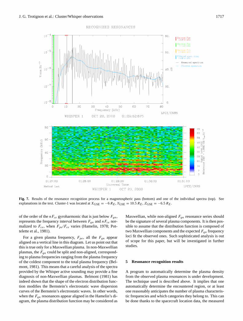
Fig. 7. Results of the resonance recognition process for a magnetospheric pass (bottom) and one of the individual spectra (top). Seeexplanations in the text. Cluster-1 was located atXGSE = −6RE , YGSE = 10.5RE , ZGSE = −6.5RE .

of the order of thenFce gyroharmonic that is just belowFqn,represents the frequency interval betweenFqn andnFce nor-malized toFce, whenFpe/Fce varies (Hamelin, 1978; Pot-telette et al., 1981).

For a given plasma frequency,Fpe, all the Fqn appearaligned on a vertical line in this diagram. Let us point out thatthis is true only for a Maxwellian plasma. In non-Maxwellianplasmas, theFqn could be split and non-aligned, correspond-ing to plasma frequencies ranging from the plasma frequencyof the coldest component to the total plasma frequency (Bel-mont, 1981). This means that a careful analysis of the spectraprovided by the Whisper active sounding may provide a finediagnosis of non-Maxwellian plasmas. Belmont (1981) hasindeed shown that the shape of the electron distribution func-tion modifies the Bernstein’s electrostatic wave dispersioncurves of the Bernstein’s electrostatic waves. In other words,when theFqn resonances appear aligned in the Hamelin’s di-agram, the plasma distribution function may be considered as

Maxwellian, while non-alignedFqn resonance series shouldbe the signature of several plasma components. It is then pos-sible to assume that the distribution function is composed oftwo Maxwellian components and the expectedFqn frequencyloci fit the observed ones. Such sophisticated analysis is outof scope for this paper, but will be investigated in furtherstudies.

5 Resonance recognition results

A program to automatically determine the plasma densityfrom the observed plasma resonances is under development.The technique used is described above. It implies that oneautomatically determine the encountered region, or at leastone reasonably anticipates the number of plasma characteris-tic frequencies and which categories they belong to. This canbe done thanks to the spacecraft location data, the measured

1718 J. G. Trotignon et al.: Cluster/Whisper observations

magnetic fields (Balogh et al., 1997), and a magnetospheremodel (Kosik, 1998). We have to know if the spacecraft iseither in the solar wind, the magnetosheath, the outer mag-netosphere, the plasmasphere, the cusp regions, or in the fartail. Although it is not positively required, the diagnosis ismore precise and reliable whenever the encountered regionis known and the appropriate resonance recognition processis applied. Here are some results for the differentFpe/Fce

ratios.The bottom panel in Fig. 5 shows the recognized reso-

nances superimposed on the electric field spectra measuredby Whisper on 9 September 2000. This measured spectro-gram is the same as the one that is shown at the top of Fig. 2.The lowest black line, close to 20 kHz, is the recognized elec-tron gyrofrequency,Fce. The second black line, just aboveFce, stands for the computed plasma frequency,Fpe. It isobtained from the best fit of the theoretical Berntein’s modefrequencies,Fqn, which are aligned in the Hamelin’s dia-gram, to the observedFqn resonances. The upper hybrid fre-quency,Fuh, derived from the computedFce andFpe values,is shown by the third black line, while the upper two blacklines are theFq2 andFq3 given by the program. Finally, themaximum intensities of the smoothed spectra are plotted inpurple. Except for some erroneous identifications at the endof the period, the program turns out to work satisfactorily. AsFpe andFce are found to be 25–45 kHz and 20 kHz, respec-tively, we can conclude that in this region, the plasma densityand magnetic field modulus are of the order of 8–25 cm−3

and 700 nT, respectively.An individual spectrum acquired at 23:58:24 UT on the

same day (this spectrum is also shown in Fig. 3) is displayedat the top of Fig. 5 with the computed resonances.Fpe andFce are found to be 27.7 kHz (red vertical line) and 20.3 kHz(green vertical solid line), respectively; these values corre-spond to a density of 9.5 cm−3 and a magnetic field inten-sity of 725 nT. As can be seen, the orange vertical line thatgives the expectedFuh does not coincide with the peak thatis observed 2 kHz above. Let us also remark that no strongresonance seems to be associated with the derivedFpe; thisis often the case. TheFuh andFpe resonances are sometimesobserved, either both or separately, and sometimes they arenot seen at all. Further investigations will be necessary in or-der to comment further about these behaviours. Finally, theblue vertical line is the maximum of the smoothed spectrumthat is represented as a blue wavy line, and the two violetvertical dashed lines are the obtainedFq2 andFq3.

Figures 6 and 7 confirm that the resonance recognitionprocess works efficiently in the magnetosphere whenFce issmall (3.2 kHz and 1.1 kHz, respectively,) andFpe/Fce is ei-ther low or high ( 2.5 and 9.6, respectively). Incidentally, it isimportant to note here that the smoothed spectrum maximum(blue vertical line in the top panels of Figs. 6 and 7) is alwaysabove the plasma frequency (red vertical line in Fig. 6 and or-ange line in Fig. 7, the latter actually covers the red one). Letus recall that the frequency location of this maximum is usedas an initial value (upper value) for the plasma frequency de-termination process (see Sect. 3).

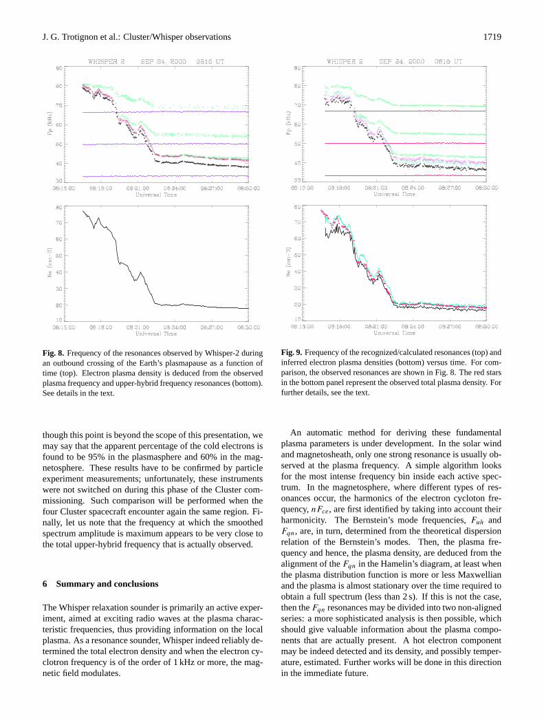
On 24 September 2000, during the spacecraft commis-sioning phase, Cluster-2 crossed the plasmapause twice,round 07:05 UT and 08:19 UT. The resonances triggered byWhisper-2 around 08:19 UT are shown in the top panel ofFig. 8, when Cluster-2 was leaving the Earth’s plasmasphereand it entered the magnetosphere at 08:22 UT. At 08:19 UT,salsa was located atXGSE = 3.16RE , YGSE = −2.0RE ,ZGSE = 1.6RE , whereRE is the Earth’s radius and GSE de-notes the geocentric solar ecliptic coordinate system. TheL and invariant latitude were 5.3 and 64.4◦, respectively,which is common for the dayside plasmapause (Chappell etal., 1971). The purple lines connect the observed 2Fce, 3Fce,and 4Fce resonances; the green diamonds stand for theFq2,Fq3, andFq4; the red triangles representFuh, while the blackstars denote the frequency location of the resonance calledFx

by Belmont (1981). Finally, the black crosses are theFuh fre-quency calculated from theFce andFx measured values. Ascan be seen, black crosses and red triangles almost merge, asexpected, ifFx is the plasma frequency. The electron densityderived from theFx andFuh observations is also displayedas a function of time in the bottom panel of Fig. 8.

The resonance recognition technique described above hasbeen applied to the 24 September 2000 plasmapause cross-ing event shown in Fig. 8. The recognized resonances are dis-played at the top of Fig. 9: the quasi-horizontal red lines con-nect the calculated gyroharmonicsnFce and the green dia-monds denote the calculated Bernstein’s resonancesFqn. Al-though several Bernstein’s resonances are actually observedbetween two successive harmonics ofFce, as shown in thetop panel of Fig. 8, only one is given by the resonance recog-nition programme, since we are looking for the series ofBernstein’s resonances that are aligned in the Hamelin’s di-agram. The relative plasma frequency, here calledFal forconvenience, and the associated upper-hybrid frequencyFuh

are plotted as black stars and purple triangles, respectively,in the top panel of Fig. 9. The blue crosses stand for the fre-quency locations of the smoothed spectrum maxima, whichare used as upper estimates of the plasma frequency in the au-tomatic recognition process. Three estimates of the electronplasma density can thus be provided; they are plotted in thebottom panel of Fig. 9. The black line is the density calcu-lated from the alignment of the Bernstein’s resonances in theHamelin’s diagram, the blue line is the density given by thesmoothed spectrum maxima, and the red stars are the den-sities deduced from theFx observations. The latter curve issimilar to the one that is plotted as a black line at the bottomof Fig. 8. As can be seen, the assumption that the smoothedspectrum maxima occur most of the time above the plasmafrequency is valid. Another significant result is that theFal

value derived from the Bernstein’s resonances alignment inthe Hamelin’s diagram is always below the observedFx . It isworth recalling that Belmont (1981) and Etcheto et al. (1983)have demonstrated thatFal corresponds to the cold electronpopulation, whileFx relates to the total electron population,the latter resonance being the only one actually observed.This is corroborated here by the existence of a non-alignedBernstein’s resonance series (not shown in the paper). Al-

J. G. Trotignon et al.: Cluster/Whisper observations 1719

Fig. 8. Frequency of the resonances observed by Whisper-2 duringan outbound crossing of the Earth’s plasmapause as a function oftime (top). Electron plasma density is deduced from the observedplasma frequency and upper-hybrid frequency resonances (bottom).See details in the text.

though this point is beyond the scope of this presentation, wemay say that the apparent percentage of the cold electrons isfound to be 95% in the plasmasphere and 60% in the mag-netosphere. These results have to be confirmed by particleexperiment measurements; unfortunately, these instrumentswere not switched on during this phase of the Cluster com-missioning. Such comparison will be performed when thefour Cluster spacecraft encounter again the same region. Fi-nally, let us note that the frequency at which the smoothedspectrum amplitude is maximum appears to be very close tothe total upper-hybrid frequency that is actually observed.

6 Summary and conclusions

The Whisper relaxation sounder is primarily an active exper-iment, aimed at exciting radio waves at the plasma charac-teristic frequencies, thus providing information on the localplasma. As a resonance sounder, Whisper indeed reliably de-termined the total electron density and when the electron cy-clotron frequency is of the order of 1 kHz or more, the mag-netic field modulates.

Fig. 9. Frequency of the recognized/calculated resonances (top) andinferred electron plasma densities (bottom) versus time. For com-parison, the observed resonances are shown in Fig. 8. The red starsin the bottom panel represent the observed total plasma density. Forfurther details, see the text.

An automatic method for deriving these fundamentalplasma parameters is under development. In the solar windand magnetosheath, only one strong resonance is usually ob-served at the plasma frequency. A simple algorithm looksfor the most intense frequency bin inside each active spec-trum. In the magnetosphere, where different types of res-onances occur, the harmonics of the electron cycloton fre-quency,nFce, are first identified by taking into account theirharmonicity. The Bernstein’s mode frequencies,Fuh andFqn, are, in turn, determined from the theoretical dispersionrelation of the Bernstein’s modes. Then, the plasma fre-quency and hence, the plasma density, are deduced from thealignment of theFqn in the Hamelin’s diagram, at least whenthe plasma distribution function is more or less Maxwellianand the plasma is almost stationary over the time required toobtain a full spectrum (less than 2 s). If this is not the case,then theFqn resonances may be divided into two non-alignedseries: a more sophisticated analysis is then possible, whichshould give valuable information about the plasma compo-nents that are actually present. A hot electron componentmay be indeed detected and its density, and possibly temper-ature, estimated. Further works will be done in this directionin the immediate future.

1720 J. G. Trotignon et al.: Cluster/Whisper observations

Finally, it is worth pointing out that a careful and accuratedetermination of the characteristic frequencies of the encoun-tered plasmas is fundamental to interpreting observed naturalwaves. This is, for example, the only way to reliably identifycutoff frequencies or wave excitation maxima and hence, todetermine the modes in which the natural waves are actuallypropagating (see, for example, Decreau et al., 2001, this issueand Canu et al., 2001, this issue). We must also keep in mindthat the density determination that relies on natural waves orspacecraft potential measurements cannot be considered ascompletely reliable. As said above, a misinterpretation is of-ten possible when no cross-check with an active experimentis done.

Acknowledgement.We are very grateful to E. Guyot, L. Launay,and J.-L. Fousset who have developed most of the Whisper data pro-cessing tools. We would like also to thank H. Poussin, M. Nonon-Latapie, D. Delmas, H. Marquier, K. Amsif, D. Gras, J.-P. Thou-venin, and J.-Y. Prado from CNES for their effective support.

The Editor in Chief thanks two referees for their help in eval-uating this paper.

References

Balogh, A., Dunlop, M. W., Cowley, S. W. H., Southwood, D. J.,Thomlinson, J. G., Glassmeier, K. H., Musmann, G., Luhr, H.,Buchert, S., Acuna, M. H., Fairfield, D. H., Slavin, J. A., Riedler,W., Schwingenschuh, K., Kivelson, M. G., and the Cluster mag-netometer team: The Cluster magnetic field investgation, SpaceSci. Rev., 79, 65–91, 1997.

Belmont, G.: Characteristic frequencies of a non-Maxwellianplasma: a method for localizing the exact frequencies of mag-netospheric intense natural waves nearFpe, Planet. Space Sci.,29, 1251–1266, 1981.

Belmont, G., Canu, P., Etcheto, J., de Feraudy, H., Higel, B., Pot-telette, R., Beghin, C., Debrie, R., Decreau, P. M. E., Hamelin,M., and Trotignon, J. G.: Advances in magnetospheric plasmadiagnosis by active experiments, in Proc. Conf. Achievements ofthe IMS, 26–28 June 1984, Graz, Austria, ESA SP-217, 695–699, 1984.

Bernstein, I. B.: Waves in a plasma in a magnetic field, Phys. Rev.,109, 10–21, 1958.

Canu, P., Decreau, P., Trotignon, J. G., Rauch, J. L., Seran, H. C.,Fergeau, P., Leveque, M., Martin, Ph., Sene, F. X., Le Guirriec,E., Alleyne, H., and Yearby, K.: Identification of natural plasmaemissions with the Whisper relaxation sounder, Ann. Geophysi-cae, 2001, this issue.

Chappell, C. R., Harris, K. K., and Sharp, G. W.: The dayside ofthe plasmasphere, J. Geophys. Res., 76, 7632–7647, 1971.

Decreau, P. M. E., Fergeau, P., Krasnoselskikh, V., Leveque, M.,Martin, Ph., Randriamboarison, O., Sene, F. X., Trotignon, J. G.,Canu, P., Mogensen, P. B., and Whisper Investigators: Whisper,a resonance sounder and wave analyser: performances and per-spectives for the Cluster mission, Space Sci. Rev., 79, 157–193,1997.

Decreau, P. M. E., Fergeau, P., Krasnoselskikh, V., Le Guirriec,

E., Leveque, M., Martin, Ph., Randriamboarison, O., Rauch, J.L., Sene, F. X., Seran, H. C., Trotignon, J. G., Canu, P., Cornil-leau, N., De Feraudy, H., Alleyne, H., Yearby, K., Woolliscroft,L., Mogensen, P. B., Gustafsson, G., Andre, M., Gurnett, D. C.,Darrouzet, F., and Whisper experimenters: Early results from theWhisper instrument on Cluster: an overview, Ann. Geophysicae,2001, this issue.

Etcheto, J., de Feraudy, H., and Trotignon, J. G.: Plasma reso-nance stimulation in space plasmas, Adv. Space Res., 1, 183–196, 1981.

Etcheto, J., Belmont, G., Canu, P., and Trotignon, J. G.: Activesounder experiments on GEOS and ISEE, in Active experimentsin space symposium, 24–29 May 1983, Alpbach, ESA SP-195,39–46, 1983.

Gurnett, D. A.: Principles of space plasma wave instrument de-sign, in: Measurement techniques in space plasmas: fields, (Eds)Pfaff, R. F., Borovsky, J. E., and Young, D. T., American Geo-physical Union, USA, pp. 121–136, 1998.

Gustafsson, G., Bostrom, R., Holback, B., Holmgren, G., Lundgren,A., Stasiewicz, K.,Ahlen, L., Mozer, F. S., Pankow, D., Harvey,P., Berg, P., Ulrich, R., Pedersen, A., Schmidt, R., Butler, A.,Fransen, A. W. C., Klinge, D., Thomsen, M., Falthammar, C.-G.,Lindqvist, P.-A., Christenson, S., Holtet, J., Lybekk, B., Sten, T.A., Tanskanen, P., Lappalainen, K., and Wygant, J.: The electricfield and wave experiment for the Cluster mission, Space Sci.Rev., 79, 137–156, 1997.

Hamelin, M.: Contributiona l’etude des ondeselectrostatiques etelectromagnetiques au voisinage de la frequence hybride bassedans le plasma ionospherique, These de Doctorat d’Etat, Univer-site d’Orleans, Orleans, France, 1978.

Kosik, J. C.: A quantitative model of the magnetosphere withpoloidal vector fields, Ann. Geophysicae, 16, 1557–1566, 1998.

Lefeuvre, F., Roux, A., de la Porte, B., Dunford, C., Woolliscroft,L. C. C., Davies, P. N. H., Davis, S. J., and Gough, M. P.: TheWave Experiment Consortium, in Cluster: mission, payload andsupporting activities, ESA SP-1159, 5–15, 1993.

Perraut, S., de Feraudy, H., Roux, A., Decreau, P. M. E., Paris,J., and Matson, L.: Density measurements in key regions ofthe Earth’s magnetosphere: cusp and auroral region, J. Geophys.Res., 95, 5997–6014, 1990.

Pottelette, R., Hamelin, M., Illiano, J. M., and Lembege, B. L.:Interpretation of the fine structure of electrostatic waves excitedin space, Phys. Fluids, 24, 1517–1526, 1981.

Tataronis, J. A. and Crawford, F. W.: Cyclotron harmonic wavepropagation and instabilities: I. perpendicular propagation, J.Plasma Phys., 4, 231–248, 1970.

Thouvenin, J. P. and Trotignon, J. G.: Automatic resonance recog-nition method in solar wind, Nuovo Ciment. Soc. Ital. Fis., C, 3,696–710, 1980.

Trotignon, J. G., Etcheto, J., and Thouvenin, J. P.: Automatic de-termination of the electron density measured by the relaxationsounder on board ISEE-1, J. Geophys. Res., 91, 4302–4320,1986.

Woolliscroft, L. J. C., Alleyne, H. ST. C., Dunford, C. M., Sumner,A., Thomson, J. A., Walker, S. N., Yearby, K. H., Buckley, A.,Chapman, S., Gough, M. P., and the DWP Co-Investigators: Thedigital wave-processing experiment on Cluster, Space Sci. Rev.,79, 209–231, 1997.