Psychological ScienceXX(X) 1 –10© The Author(s) 2013Reprints and permissions: sagepub.com/journalsPermissions.navDOI: 10.1177/0956797613495418pss.sagepub.com

General Article

Should the human mind be seen as an engine of proba-bilistic inference, yielding optimal or near-optimal per-formance, as several recent prominent articles have suggested (Frank & Goodman, 2012; Gopnik, 2012; Téglás et al., 2011; Tenenbaum, Kemp, Griffiths, & Goodman, 2011)? Tenenbaum et al. (2011) argued that “over the past decade, many aspects of higher-level cog-nition have been illuminated by the mathematics of Bayesian statistics” (pp. 1279–1280), pointing to treat-ments of language; memory; sensorimotor systems; judg-ments of causal strength; diagnostic and conditional reasoning; human notions of similarity, representative-ness, and randomness; and predictions about the future of everyday events.

In support of this view, researchers have combined experimental data with precise, elegant models that pro-vide remarkably good quantitative fits. For example, Xu and Tenenbaum (2007) presented a well-motivated prob-abilistic model “based on principles of rational statistical inference” (p. 246) that closely fit adults’ and children’s generalization of novel words to categories at different levels of abstraction (e.g., “green pepper” vs. “pepper” vs. “vegetable”) as a function of how labeled examples of those categories were distributed.

In these models, cognition is viewed as a process of drawing inferences from observed data in a fashion nor-matively justified by mathematical probability theory. In

probability theory, this kind of inference is governed by Bayes’s law. Let D be the data and H

1 through H

k be

hypotheses; assume that it is known that exactly one of the hypotheses is true. Bayes’s law states that for each hypothesis,

p Dp D p

p D pi

i i

j j

j

k( | )( | ) ( )

( | ) ( )H

H H

H H= ⋅

⋅=∑

1

In this equation, p(Hi|D) is the posterior probability of

the hypothesis Hi given that the data D have been

observed; p(Hi) is the prior probability that H

i is true

before any data have been observed; and p(D|Hi) is the

likelihood, the conditional probability that D would be observed assuming that H

i is true. The formula states that

the posterior probability is proportional to the product of the prior probability and the likelihood. In most of the models that we discuss in this article, the “data” are infor-mation available to a human reasoner, the “priors” are a characterization of the reasoner’s initial state of knowl-edge, and the “hypotheses” are the conclusions that he or

495418 PSSXXX10.1177/0956797613495418Marcus, DavisAre Probabilistic Models of Higher-Level Cognition Robust?research-article2013

Corresponding Author:Gary F. Marcus, Department of Psychology, New York University, 6 Washington Place, New York, NY 10003 E-mail: gary.marcus@nyu.edu

How Robust Are Probabilistic Models of Higher-Level Cognition?

Gary F. Marcus and Ernest DavisNew York University

AbstractAn increasingly popular theory holds that the mind should be viewed as a near-optimal or rational engine of probabilistic inference, in domains as diverse as word learning, pragmatics, naive physics, and predictions of the future. We argue that this view, often identified with Bayesian models of inference, is markedly less promising than widely believed, and is undermined by post hoc practices that merit wholesale reevaluation. We also show that the common equation between probabilistic and rational or optimal is not justified.

Keywordscognition(s), Bayesian models, optimality

Received 1/8/13; Revision accepted 5/27/13

Psychological Science OnlineFirst, published on October 1, 2013 as doi:10.1177/0956797613495418

2 Marcus, Davis

she draws. For example, in a word-learning task, the data could be observations of language, and a hypothesis could be a conclusion that the word dog denotes a par-ticular category of object (friendly, furry animals that bark).

Couching their theory in the language of evolution and adaptation, Tenenbaum et al. (2011) argued that “the Bayesian approach [offers] a framework for understand-ing why the mind works the way it does, in terms of rational inference adapted to the structure of real-world environments” (p. 1285).

To date, these models have been criticized only rarely (Bowers & Davis, 2012; Eberhardt & Danks, 2011; Jones & Love, 2011). Here, through a series of detailed case studies, we demonstrate that two closely related problems—one of task selection, the other of model selection—undermine the conclusions that have been drawn about whether cog-nition is in fact either optimal or driven by probabilistic inference. Furthermore, we show that multiple probabilistic models (some compatible with the observed data but oth-ers not) are often potentially applicable to any given task, that published claims of fits of probabilistic models some-times depend on post hoc choices that are unprincipled, and that, in many cases, extant models depend on assump-tions that are empirically false, nonoptimal, or both.

Task Selection

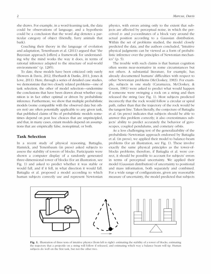
In a recent study of physical reasoning, Battaglia, Hamrick, and Tenenbaum (in press) asked subjects to assess the stability of towers of blocks. Participants were shown a computer display of a randomly generated three-dimensional tower of blocks (for an illustration, see Fig. 1) and asked to predict whether it was stable or would fall, and if it fell, in what direction it would fall. Battaglia et al. proposed a model according to which human subjects correctly use and represent Newtonian

physics, with errors arising only to the extent that sub-jects are affected by perceptual noise, in which the per-ceived x- and y-coordinates of a block vary around the actual position according to a Gaussian distribution. Within the set of problems studied, the model closely predicted the data, and the authors concluded, “Intuitive physical judgments can be viewed as a form of probabi-listic inference over the principles of Newtonian mechan-ics” (p. 5).

The trouble with such claims is that human cognition often seems near-normative in some circumstances but not others. A substantial literature, for example, has already documented humans’ difficulties with respect to other Newtonian problems (McCloskey, 1983). For exam-ple, subjects in one study (Caramazza, McCloskey, & Green, 1981) were asked to predict what would happen if someone were swinging a rock on a string and then released the string (see Fig. 1). Most subjects predicted incorrectly that the rock would follow a circular or spiral path, rather than that the trajectory of the rock would be the tangent line. Taken literally, the conjecture of Battaglia et al. (in press) indicates that subjects should be able to answer this problem correctly; it also overestimates sub-jects’ ability to predict accurately the behavior of gyro-scopes, coupled pendulums, and cometary orbits.

As a less challenging test of the generalizability of the probabilistic-Newtonian approach endorsed by Battaglia et al. (in press), we applied their model to balance-beam problems (for an illustration, see Fig. 1). These involve exactly the same physical principles as the tower-of-blocks problems; therefore, if Battaglia et al. were cor-rect, it should be possible to account for subjects’ errors in terms of perceptual uncertainty. We applied their model (Gaussian distribution) of uncertainty to positional and mass information, both separately and combined. For a wide range of configurations, given any reasonable measure of uncertainty, the model predicted that subjects

Fig. 1.! Illustration of three tests of intuitive physics (from left to right): estimating the stability of a tower of blocks, estimating the trajectory that a projectile on a string will follow if released, and estimating which way a balance beam will tip. Human subjects do well on the first task, but not the other two.

Are Probabilistic Models of Higher-Level Cognition Robust? 3

would always answer the problem correctly (see the Supplemental Material available online).

As is well documented in the experimental literature, however, this prediction is false. Both children and many untutored adults (Siegler, 1976) frequently make a range of errors, such as relying solely on the number of weights to the exclusion of information about how far those weights are from the fulcrum. For this type of problem, which is only slightly different from the problems posed by Battaglia et al. (in press; both hinge on factors of weight, distance, and leverage), the model proposed by Battaglia et al. has a very poor fit. What held true in the specific case of their tower problems—that human per-formance is near optimal—simply is not true for a prob-lem governed by the laws of physics applied in a slightly different configuration. (Of course, the subjects in the study by Battaglia et al. were undergraduates trained at MIT, and such sophisticated subjects may do better than more typical subjects.)

The larger concern is that the probabilistic-cognition literature as a whole may disproportionately report suc-cesses, a problem akin to Rosenthal’s (1979) file-drawer problem, which would lead to a distorted perception of the applicability of the approach. Table 1 summarizes many of the most influential findings in the cognitive lit-erature on probabilistic inference and shows that, in many domains, results that fit naturally with probabilistic techniques and claims of optimality are closely paralleled by equally compelling results that do not fit so squarely. This raises important issues about the generalizability of the framework.

The risk of confirmationism is almost certainly exacer-bated by the tendency of advocates of probabilistic theo-ries of cognition (like researchers using many computational frameworks) to follow a breadth-first search strategy, in which the formalism is extended to an ever-broader range of domains (most recently, intuitive physics and intuitive psychology), rather than a depth-first strategy, in which

Table 1.! Examples of Domains in Which Performance Has Been Found to Fit Naturally With Probabilistic Explanations in Some Cases but Not Others

Domain Apparently optimal performance Apparently nonoptimal performance

Intuitive physics Tower problems (Battaglia, Hamrick, & Tenenbaum, in press)

Balance-scale problems (Siegler, 1976)Projectile-trajectory problems (Caramazza,

McCloskey, & Green, 1981)Incorporation of base

ratesVarious tasks (Frank & Goodman, 2012;

Griffiths & Tenenbaum, 2006)Base-rate neglect (Kahneman & Tversky, 1973; but

see Gigerenzer & Hoffrage, 1995)Extrapolation from

small samplesFuture prediction (Griffiths & Tenenbaum,

2006)Size principle (Tenenbaum & Griffiths, 2001a)

Anchoring (Tversky & Kahneman, 1974)Underfitting of exponentials (Timmers &

Wagenaar, 1977)Gambler’s fallacy (Tversky & Kahneman, 1974)Conjunction fallacy (Tversky & Kahneman, 1983)Estimating unique events (Khemlani, Lotstein, &

Johnson-Laird, 2012)Word learning Using sample diversity as a cue to induction

(Xu & Tenenbaum, 2007)Using sample diversity as a cue to induction

(Gutheil & Gelman, 1997)Evidence selection (Ramarajan, Vohnoutka, Kalish,

& Rhodes, 2012)Social cognition Pragmatic reasoning (Frank & Goodman, 2012) Attributional biases (Ross, 1977)

Egocentrism (Leary & Forsyth, 1987)Behavioral prediction of children (Boseovski &

Lee, 2006)Memory Rational analysis (Anderson & Schooler, 1991) Eyewitness testimony (Loftus, 1996)

Vulnerability to interference (Wickens, Born, & Allen, 1963)

Foraging Animal behavior (McNamara, Green, & Olsson, 2006)

Information foraging (Jacobs & Kruschke, 2011)

Probability matching (West & Stanovich, 2003)

Deductive reasoning Deduction (Oaksford & Chater, 2009) Deduction (Evans, 1989)! Overview Higher-level cognition (Tenenbaum, Kemp,

Griffiths, & Goodman, 2011)Higher-level cognition (Kahneman, 2003; Marcus,

2008)

4 Marcus, Davis

some challenging domain is explored in great detail with respect to a wide range of tasks. More revealing than pick-ing out arbitrary tasks in new domains might be deeper exploration of domains in which large bodies of “pro” and “anti” rationality literature are juxtaposed. For example, when people extrapolate, they are sometimes remarkably accurate, as Griffiths and Tenenbaum (2006) have shown, but at other times remarkably inaccurate, as when they anchor their judgments on arbitrary and irrelevant bits of information (Tversky & Kahneman, 1974). An attempt to understand the seemingly competing mechanisms involved might be more illuminating than the current practice of identifying a small number of tasks in each domain that seem to be compatible with a probabilistic model.

Model Selection

Closely aligned with the problem of how tasks are selected is the problem of how models are selected. Each model depends heavily on the choice of probabilities, which can come from three kinds of sources:

!" Real-world frequencies!" Experimental subjects’ judgments!" Mathematical models, such as Gaussian distribu-

tions or information-theoretic arguments

Moreover, a number of other parameters must also be set by basing the model or its parameters on real-world sta-tistics either for the problem under consideration or for some analogous problem; by basing the model or its parameters on some other psychological experiment; by choosing the model or tuning the parameters to best fit the experiment at hand; or by using purely theoretical considerations, which are sometimes quite arbitrary.

Unfortunately, each of these choices can be problem-atic. To take one example, real-world frequencies may depend very strongly on the particular data set being used, the sampling technique, or the implicit indepen-dence assumptions. For instance, Griffiths and Tenenbaum (2006) studied estimation abilities. Subjects were asked questions like “If you heard that a member of the House of Representatives had served for 15 years, what would you predict his total term in the House would be?” The authors proposed a model in which the hypotheses were the different possible total lengths of the term, the prior was the real-world distribution of the lengths of repre-sentatives’ terms, and the datum was the fact that the representative’s term of service was at least 15 years. The models for the other questions in this study were analo-gous. These models accounted very accurately for the subjects’ responses to seven of the nine questions. Griffiths and Tenenbaum concluded that “everyday cog-nitive judgments follow the . . . optimal statistical princi-ples” and there is “close correspondence between

people’s implicit probabilistic models and the statistics of the world” (p. 767).

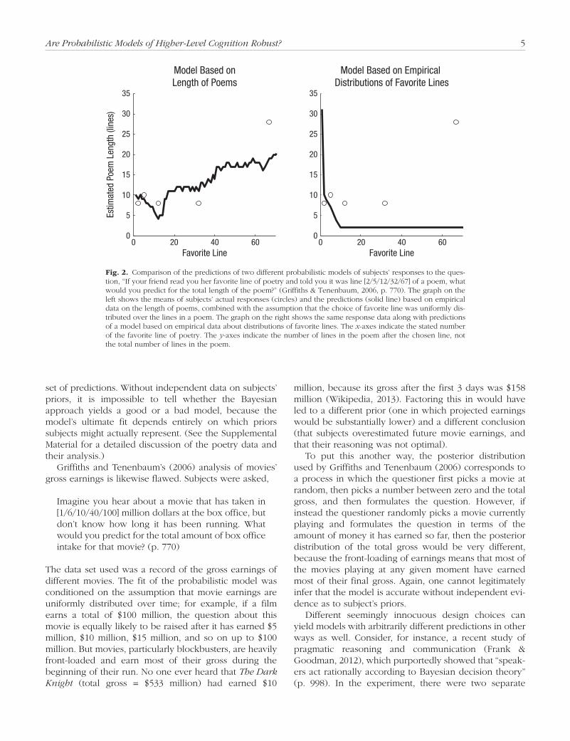
But it is important to realize that the fit of a model to the data depends heavily on how the priors are chosen. To the extent that priors may be chosen post hoc, the true fit of a model can easily be overestimated, perhaps greatly. For instance, one of the questions in Griffiths and Tenenbaum’s (2006) study was, “If your friend read you her favorite line of poetry and told you it was line [2/5/12/32/67] of a poem, what would you predict for the total length of the poem?” (p. 770). How well a model fits this datum depends on what prior is presupposed. Griffiths and Tenenbaum based their prior on the distri-bution of length in an online corpus of poetry. To this distribution, they applied a stochastic model motivated by Tenenbaum’s “size principle” (Tenenbaum & Griffiths, 2001a): The model assumed that (a) the choice of favorite line of poetry was uniformly distributed over poems in the corpus; (b) given a particular poem, the choice of favorite line was uniformly distributed over the lines in the poem; and (c) the subjects’ answer to the question was the median of the posterior distribution.

From the apparent fit, Griffiths and Tenenbaum (2006) claimed that “people’s judgements for . . . poem lengths . . . were indistinguishable from optimal Bayesian predic-tions based on the empirical prior distributions” (p. 770). They did not report a statistical analysis, but they included a diagram illustrating the fit. However, the fit between the model and the experimental results was not in fact as close as that diagram suggested. In the diagram, the y-axis represented the total length of the poem, which is the question the subjects were asked. However, it requires no great knowledge of poetry to predict that a poem whose fifth line has been quoted must have at least five lines; nor will an insurance company pay much to an actuary for predicting that a man who is currently 36 years old will live to at least age 36. The predictive part of these tasks is to estimate how much longer the poem will continue, or how much longer the man will live. If instead the remaining length of the poem is used as the y-axis, as in the left-hand panel in Figure 2, though the model has some predictive value for the data, the data are by no means “indistinguishable” from the predictions of the model.

More important, the second assumption in Griffiths and Tenenbaum’s (2006) stochastic model, that favorite lines are uniformly distributed throughout the length of a poem, is demonstrably false. An online data set of favor-ite passages of poetry (American Academy of Poets, 1997–2013) clearly reveals that favorite passages are not uniformly distributed; rather, they are generally the first or last line of a poem, and last lines are listed as favorites about twice as frequently as first lines. As illustrated in the right-hand panel of Figure 2, a model that incorpo-rated these empirical facts would yield a very different

Are Probabilistic Models of Higher-Level Cognition Robust? 5

set of predictions. Without independent data on subjects’ priors, it is impossible to tell whether the Bayesian approach yields a good or a bad model, because the model’s ultimate fit depends entirely on which priors subjects might actually represent. (See the Supplemental Material for a detailed discussion of the poetry data and their analysis.)

Griffiths and Tenenbaum’s (2006) analysis of movies’ gross earnings is likewise flawed. Subjects were asked,

Imagine you hear about a movie that has taken in [1/6/10/40/100] million dollars at the box office, but don’t know how long it has been running. What would you predict for the total amount of box office intake for that movie? (p. 770)

The data set used was a record of the gross earnings of different movies. The fit of the probabilistic model was conditioned on the assumption that movie earnings are uniformly distributed over time; for example, if a film earns a total of $100 million, the question about this movie is equally likely to be raised after it has earned $5 million, $10 million, $15 million, and so on up to $100 million. But movies, particularly blockbusters, are heavily front-loaded and earn most of their gross during the beginning of their run. No one ever heard that The Dark Knight (total gross = $533 million) had earned $10

million, because its gross after the first 3 days was $158 million (Wikipedia, 2013). Factoring this in would have led to a different prior (one in which projected earnings would be substantially lower) and a different conclusion (that subjects overestimated future movie earnings, and that their reasoning was not optimal).

To put this another way, the posterior distribution used by Griffiths and Tenenbaum (2006) corresponds to a process in which the questioner first picks a movie at random, then picks a number between zero and the total gross, and then formulates the question. However, if instead the questioner randomly picks a movie currently playing and formulates the question in terms of the amount of money it has earned so far, then the posterior distribution of the total gross would be very different, because the front-loading of earnings means that most of the movies playing at any given moment have earned most of their final gross. Again, one cannot legitimately infer that the model is accurate without independent evi-dence as to subject’s priors.

Different seemingly innocuous design choices can yield models with arbitrarily different predictions in other ways as well. Consider, for instance, a recent study of pragmatic reasoning and communication (Frank & Goodman, 2012), which purportedly showed that “speak-ers act rationally according to Bayesian decision theory” (p. 998). In the experiment, there were two separate

0 20 40 600

5

10

15

20

25

30

35

Model Based onLength of Poems

0 20 40 600

5

10

15

20

25

30

35

Model Based on Empirical Distributions of Favorite Lines

Estim

ated

Poe

m L

engt

h (li

nes)

Favorite Line Favorite Line

Fig. 2.! Comparison of the predictions of two different probabilistic models of subjects’ responses to the ques-tion, “If your friend read you her favorite line of poetry and told you it was line [2/5/12/32/67] of a poem, what would you predict for the total length of the poem?” (Griffiths & Tenenbaum, 2006, p. 770). The graph on the left shows the means of subjects’ actual responses (circles) and the predictions (solid line) based on empirical data on the length of poems, combined with the assumption that the choice of favorite line was uniformly dis-tributed over the lines in a poem. The graph on the right shows the same response data along with predictions of a model based on empirical data about distributions of favorite lines. The x-axes indicate the stated number of the favorite line of poetry. The y-axes indicate the number of lines in the poem after the chosen line, not the total number of lines in the poem.

6 Marcus, Davis

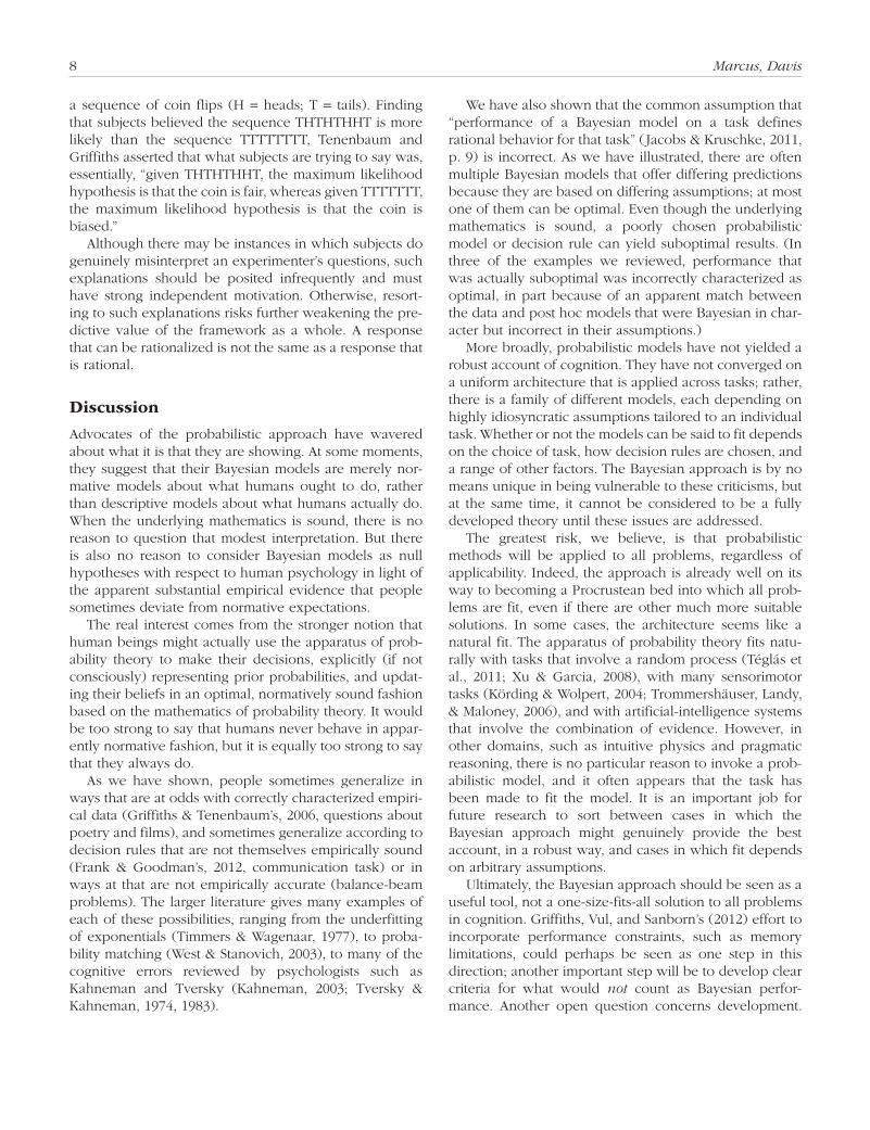
groups of subjects in two different conditions, called the “speaker” condition and the “listener” condition. (A third group, in the “salience” condition, is irrelevant to the dis-cussion here; see the Supplemental Material for details.) Subjects in the listener condition were shown a set of three objects (see Fig. 3) and asked to bet on which object a speaker would mean if he or she used a particu-lar word to refer to one of the objects (e.g., blue or circle).

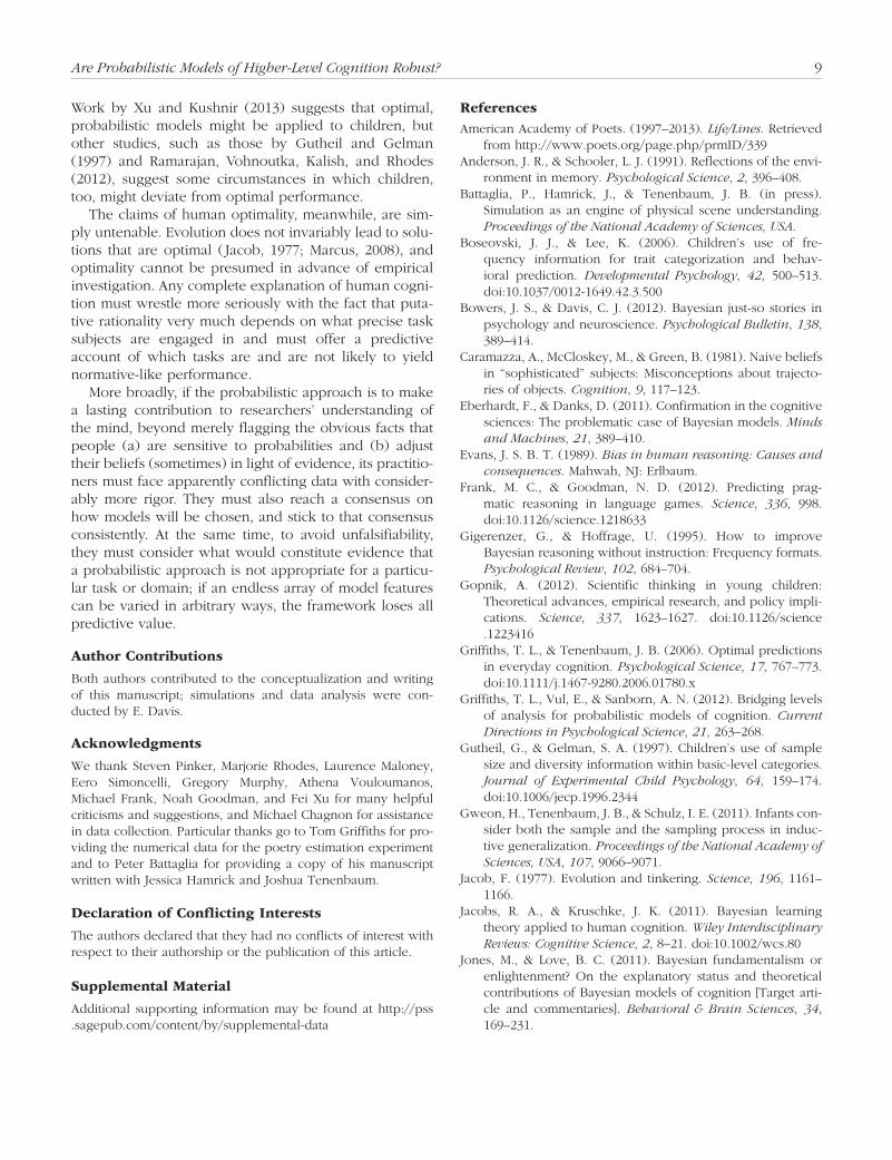
Frank and Goodman (2012) showed that a probabilis-tic “rational actor” model of the speaker, with utility defined in terms of surprisal (a measure of the informa-tion gained by the hearer) could predict subjects’ perfor-mance with near-perfect accuracy (Fig. 4, left panel). The trouble is, their model depended critically on the assump-tion that listeners believe speakers follow a decision rule

according to which they choose to use a word with a probability proportional to the word’s specificity. In the case of the set shown in Figure 3, blue has a specificity of .5, because it applies to two objects, and circle has a specificity of 1, because it applies to only one object; therefore, speakers who wish to specify the middle object would use circle two thirds of the time and blue one third of the time. Although this decision rule is not uncommon, Frank and Goodman might just as easily have chosen a model with a winner-take-all decision rule, following the maximum-expected-utility principle, which is the standard rule in decision theory. According to the winner-take-all rule, listeners expect speakers to always use the applicable word of greatest specificity; this would be circle if the middle object were intended. As Figure 4 shows, although the model with Frank and Goodman’s decision rule yielded a good fit to the data, other models, which are actually more justifiable a priori, would have yielded dramatically poorer fits. Details of the analysis are given in the Supplemental Material.

Experimenters’ choice of how to word the questions posed to subjects can also affect model fit. For example, rather than asking subjects which word they would be more likely to use in a given situation (which seems eco-logically natural), Frank and Goodman (2012) asked sub-jects in the speaker condition,

Fig. 3.! Illustration of the set of objects used in Frank and Goodman’s (2012) study. Subjects in the listener condition were asked to place a bet on which object a speaker meant if he or she used a particular word (e.g., blue or circle) to refer to one of the objects.

20

0

20

0

20

0

Frank and Goodman’s Model Mixed ModelModel With OptimalDecision Rule

40

60

80

100

40

60

80

100

40

60

80

100

Amou

nt B

et ($

)

Fig. 4.! Analysis of the effect of varying decision rules on the fit of probabilistic models to the data in Frank and Goodman’s (2012) study. Each graph shows the mean amount subjects (listeners) bet that a speaker who used the word blue was referring to each of the items in the set illustrated on the x-axis, along with the predictions (solid lines) of a different model. The left panel shows the predictions for listeners’ responses using Frank and Goodman’s suboptimal model, in which listeners use a proportional decision rule and assume that speakers use a proportional decision rule. The center panel shows the predictions of a model in which listeners use a winner-take-all rule and assume that speakers use a winner-take-all rule, which is optimal. The right panel shows the predictions of a model in which listeners assume that speakers follow a proportional decision rule, but listeners follow a winner-take-all rule. As shown, the fit of the model varies considerably depending on the post hoc choice of decision rule. Error bars on the data points represent 95% confidence intervals for the empirical data.

Are Probabilistic Models of Higher-Level Cognition Robust? 7

Imagine that you have $100. You should divide your money between the possible words—the amount of money you bet on each option should correspond to how likely you would be to use that word. Bets must sum to 100! (M. C. Frank, personal communication, September 21, 2012)

In effect, subjects were asked to place a bet on what they themselves would say. The question was ecologically anomalous and coercive in that the phrasing “should divide” placed a task demand such that all-or-none-answers were pragmatically discouraged. Had subjects instead been asked, for example, whether they would use blue or circle if they were talking to someone and wanted to refer to the middle object in the set shown in Figure 3, we suspect that 100% (rather than the 67% observed) would have answered “circle” (saying “blue” would be a violation of Gricean constraints, and an actual hearer would object that this word was ambiguous or misleading).

Table 2 enumerates some of the features that have varied empirically (without a strong a priori theoretical basis) across probabilistic models of human cognition. Individual researchers are free to tinker, but the collective enterprise suffers if choices across domains and tasks are unprincipled and inconsistent. Models that have been fit

only to one particular set of data have little value if their assumptions cannot be verified independently; in that case, the entire framework risks becoming an exercise in squeezing round pegs into square holes. (Another vivid example of a Bayesian cognitive model with arbitrary, debatable assumptions that came to our attention too late for inclusion here concerns infants’ use of hypotheses about sampling techniques. This study, by Gweon, Tenenbaum, & Schulz, 2011, is discussed at length in the Supplemental Material.)

At the extreme, when all other methods for explaining subjects’ errors as arising through optimal Bayesian rea-soning have failed, theorists have in some cases decided that subjects were actually correctly answering a question other than the one the experimenter asked. For example Oaksford and Chater (2009) explained errors in the well-known Wason card-selection task by positing that the subjects assumed the distribution of symbols on cards that would occur in a naturalistic setting; Oaksford and Chater argued that under that assumption, subjects’ answers were in fact optimal. At first glance, this seems to offer a way of rescuing optimality, but in reality, it just shifts the locus of nonoptimality elsewhere, to the pro-cess of language comprehension.

Tenenbaum and Griffiths (2001b) adopted much the same strategy in an analysis of subjects’ expectations for

Table 2.! Features That Have Varied Across Probabilistic Models of Human Cognition

Study Domain Probabilities incorporated and their derivationDecision

rule

Battaglia, Hamrick, & Tenenbaum (in press)

Intuitive physics Form of the distribution of block position: theoretically derived (Gaussian, corrected for interpenetration)

Mean block position: empirically derivedStandard deviation of block position: tuned

post hoc

Maximum probability

Frank & Goodman (2012)

Pragmatic reasoning with respect to communication

Probability that a particular word will be chosen for a given object: derived from an information-theoretic model and confirmed by experiment

Prior probability that an object will be referred to: experimentally derived

Proportional

Griffiths & Tenenbaum (2006)

Future predictions (“everyday cognition”)

Distribution of examples except waiting: empirically derived

Distribution of the waiting example: derived from an inverse power law tuned to fit subjects’ responses

Median

Xu & Tenenbaum (2007) Word learning Priors on semantic categories and conditionals that an entity is in a category: derived from a complex model applied to experimentally derived dissimilarity judgments

Maximum probability

Note: Even in this relatively small sample of probabilistic models, model construction is based on a wide range of techniques, potentially cho-sen post hoc from a wider range of possible options. Many of the models in these studies would have yielded poorer fits if priors had been derived differently or if different decision rules had been invoked (see, e.g., the discussion of Frank & Goodman, 2012, in the text).

8 Marcus, Davis

a sequence of coin flips (H = heads; T = tails). Finding that subjects believed the sequence THTHTHHT is more likely than the sequence TTTTTTTT, Tenenbaum and Griffiths asserted that what subjects are trying to say was, essentially, “given THTHTHHT, the maximum likelihood hypothesis is that the coin is fair, whereas given TTTTTTT, the maximum likelihood hypothesis is that the coin is biased.”

Although there may be instances in which subjects do genuinely misinterpret an experimenter’s questions, such explanations should be posited infrequently and must have strong independent motivation. Otherwise, resort-ing to such explanations risks further weakening the pre-dictive value of the framework as a whole. A response that can be rationalized is not the same as a response that is rational.

Discussion

Advocates of the probabilistic approach have wavered about what it is that they are showing. At some moments, they suggest that their Bayesian models are merely nor-mative models about what humans ought to do, rather than descriptive models about what humans actually do. When the underlying mathematics is sound, there is no reason to question that modest interpretation. But there is also no reason to consider Bayesian models as null hypotheses with respect to human psychology in light of the apparent substantial empirical evidence that people sometimes deviate from normative expectations.

The real interest comes from the stronger notion that human beings might actually use the apparatus of prob-ability theory to make their decisions, explicitly (if not consciously) representing prior probabilities, and updat-ing their beliefs in an optimal, normatively sound fashion based on the mathematics of probability theory. It would be too strong to say that humans never behave in appar-ently normative fashion, but it is equally too strong to say that they always do.

As we have shown, people sometimes generalize in ways that are at odds with correctly characterized empiri-cal data (Griffiths & Tenenbaum’s, 2006, questions about poetry and films), and sometimes generalize according to decision rules that are not themselves empirically sound (Frank & Goodman’s, 2012, communication task) or in ways at that are not empirically accurate (balance-beam problems). The larger literature gives many examples of each of these possibilities, ranging from the underfitting of exponentials (Timmers & Wagenaar, 1977), to proba-bility matching (West & Stanovich, 2003), to many of the cognitive errors reviewed by psychologists such as Kahneman and Tversky (Kahneman, 2003; Tversky & Kahneman, 1974, 1983).

We have also shown that the common assumption that “performance of a Bayesian model on a task defines rational behavior for that task” ( Jacobs & Kruschke, 2011, p. 9) is incorrect. As we have illustrated, there are often multiple Bayesian models that offer differing predictions because they are based on differing assumptions; at most one of them can be optimal. Even though the underlying mathematics is sound, a poorly chosen probabilistic model or decision rule can yield suboptimal results. (In three of the examples we reviewed, performance that was actually suboptimal was incorrectly characterized as optimal, in part because of an apparent match between the data and post hoc models that were Bayesian in char-acter but incorrect in their assumptions.)

More broadly, probabilistic models have not yielded a robust account of cognition. They have not converged on a uniform architecture that is applied across tasks; rather, there is a family of different models, each depending on highly idiosyncratic assumptions tailored to an individual task. Whether or not the models can be said to fit depends on the choice of task, how decision rules are chosen, and a range of other factors. The Bayesian approach is by no means unique in being vulnerable to these criticisms, but at the same time, it cannot be considered to be a fully developed theory until these issues are addressed.

The greatest risk, we believe, is that probabilistic methods will be applied to all problems, regardless of applicability. Indeed, the approach is already well on its way to becoming a Procrustean bed into which all prob-lems are fit, even if there are other much more suitable solutions. In some cases, the architecture seems like a natural fit. The apparatus of probability theory fits natu-rally with tasks that involve a random process (Téglás et al., 2011; Xu & Garcia, 2008), with many sensorimotor tasks (Körding & Wolpert, 2004; Trommershäuser, Landy, & Maloney, 2006), and with artificial-intelligence systems that involve the combination of evidence. However, in other domains, such as intuitive physics and pragmatic reasoning, there is no particular reason to invoke a prob-abilistic model, and it often appears that the task has been made to fit the model. It is an important job for future research to sort between cases in which the Bayesian approach might genuinely provide the best account, in a robust way, and cases in which fit depends on arbitrary assumptions.

Ultimately, the Bayesian approach should be seen as a useful tool, not a one-size-fits-all solution to all problems in cognition. Griffiths, Vul, and Sanborn’s (2012) effort to incorporate performance constraints, such as memory limitations, could perhaps be seen as one step in this direction; another important step will be to develop clear criteria for what would not count as Bayesian perfor-mance. Another open question concerns development.

Are Probabilistic Models of Higher-Level Cognition Robust? 9

Work by Xu and Kushnir (2013) suggests that optimal, probabilistic models might be applied to children, but other studies, such as those by Gutheil and Gelman (1997) and Ramarajan, Vohnoutka, Kalish, and Rhodes (2012), suggest some circumstances in which children, too, might deviate from optimal performance.

The claims of human optimality, meanwhile, are sim-ply untenable. Evolution does not invariably lead to solu-tions that are optimal ( Jacob, 1977; Marcus, 2008), and optimality cannot be presumed in advance of empirical investigation. Any complete explanation of human cogni-tion must wrestle more seriously with the fact that puta-tive rationality very much depends on what precise task subjects are engaged in and must offer a predictive account of which tasks are and are not likely to yield normative-like performance.

More broadly, if the probabilistic approach is to make a lasting contribution to researchers’ understanding of the mind, beyond merely flagging the obvious facts that people (a) are sensitive to probabilities and (b) adjust their beliefs (sometimes) in light of evidence, its practitio-ners must face apparently conflicting data with consider-ably more rigor. They must also reach a consensus on how models will be chosen, and stick to that consensus consistently. At the same time, to avoid unfalsifiability, they must consider what would constitute evidence that a probabilistic approach is not appropriate for a particu-lar task or domain; if an endless array of model features can be varied in arbitrary ways, the framework loses all predictive value.

Author Contributions

Both authors contributed to the conceptualization and writing of this manuscript; simulations and data analysis were con-ducted by E. Davis.

Acknowledgments

We thank Steven Pinker, Marjorie Rhodes, Laurence Maloney, Eero Simoncelli, Gregory Murphy, Athena Vouloumanos, Michael Frank, Noah Goodman, and Fei Xu for many helpful criticisms and suggestions, and Michael Chagnon for assistance in data collection. Particular thanks go to Tom Griffiths for pro-viding the numerical data for the poetry estimation experiment and to Peter Battaglia for providing a copy of his manuscript written with Jessica Hamrick and Joshua Tenenbaum.

Declaration of Conflicting Interests

The authors declared that they had no conflicts of interest with respect to their authorship or the publication of this article.

Supplemental Material

Additional supporting information may be found at http://pss .sagepub.com/content/by/supplemental-data

ReferencesAmerican Academy of Poets. (1997–2013). Life/Lines. Retrieved

from http://www.poets.org/page.php/prmID/339Anderson, J. R., & Schooler, L. J. (1991). Reflections of the envi-

ronment in memory. Psychological Science, 2, 396–408.Battaglia, P., Hamrick, J., & Tenenbaum, J. B. (in press).

Simulation as an engine of physical scene understanding. Proceedings of the National Academy of Sciences, USA.

Boseovski, J. J., & Lee, K. (2006). Children’s use of fre-quency information for trait categorization and behav-ioral prediction. Developmental Psychology, 42, 500–513. doi:10.1037/0012-1649.42.3.500

Bowers, J. S., & Davis, C. J. (2012). Bayesian just-so stories in psychology and neuroscience. Psychological Bulletin, 138, 389–414.

Caramazza, A., McCloskey, M., & Green, B. (1981). Naive beliefs in “sophisticated” subjects: Misconceptions about trajecto-ries of objects. Cognition, 9, 117–123.

Eberhardt, F., & Danks, D. (2011). Confirmation in the cognitive sciences: The problematic case of Bayesian models. Minds and Machines, 21, 389–410.

Evans, J. S. B. T. (1989). Bias in human reasoning: Causes and consequences. Mahwah, NJ: Erlbaum.

Frank, M. C., & Goodman, N. D. (2012). Predicting prag-matic reasoning in language games. Science, 336, 998. doi:10.1126/science.1218633

Gigerenzer, G., & Hoffrage, U. (1995). How to improve Bayesian reasoning without instruction: Frequency formats. Psychological Review, 102, 684–704.

Gopnik, A. (2012). Scientific thinking in young children: Theoretical advances, empirical research, and policy impli-cations. Science, 337, 1623–1627. doi:10.1126/science .1223416

Griffiths, T. L., & Tenenbaum, J. B. (2006). Optimal predictions in everyday cognition. Psychological Science, 17, 767–773. doi:10.1111/j.1467-9280.2006.01780.x

Griffiths, T. L., Vul, E., & Sanborn, A. N. (2012). Bridging levels of analysis for probabilistic models of cognition. Current Directions in Psychological Science, 21, 263–268.

Gutheil, G., & Gelman, S. A. (1997). Children’s use of sample size and diversity information within basic-level categories. Journal of Experimental Child Psychology, 64, 159–174. doi:10.1006/jecp.1996.2344

Gweon, H., Tenenbaum, J. B., & Schulz, I. E. (2011). Infants con-sider both the sample and the sampling process in induc-tive generalization. Proceedings of the National Academy of Sciences, USA, 107, 9066–9071.

Jacob, F. (1977). Evolution and tinkering. Science, 196, 1161–1166.

Jacobs, R. A., & Kruschke, J. K. (2011). Bayesian learning theory applied to human cognition. Wiley Interdisciplinary Reviews: Cognitive Science, 2, 8–21. doi:10.1002/wcs.80

Jones, M., & Love, B. C. (2011). Bayesian fundamentalism or enlightenment? On the explanatory status and theoretical contributions of Bayesian models of cognition [Target arti-cle and commentaries]. Behavioral & Brain Sciences, 34, 169–231.

10 Marcus, Davis

Kahneman, D. (2003). Maps of bounded rationality: Psychology for behavioral economics. American Economic Review, 93, 1449–1475.

Kahneman, D., & Tversky, A. (1973). On the psychology of prediction. Psychological Review, 80, 237–251.

Khemlani, S. S., Lotstein, M., & Johnson-Laird, P. (2012). The probabilities of unique events. PLoS ONE, 7(10), e45975. Retrieved from http://dx.doi.org/10.1371%2Fjournal.pone .0045975

Körding, K. P., & Wolpert, D. M. (2004). Bayesian integration in sensorimotor learning. Nature, 427, 244–247.

Leary, M. R., & Forsyth, D. R. (1987). Attributions of responsi-bility for collective endeavors. Review of Personality and Social Psychology, 8, 167–188.

Loftus, E. F. (1996). Eyewitness testimony. Cambridge, MA: Harvard University Press.

Marcus, G. F. (2008). Kluge: The haphazard construction of the human mind. Boston, MA: Houghton Mifflin.

McCloskey, M. (1983). Intuitive physics. Scientific American, 248(4), 114–122.

McNamara, J. M., Green, R. F., & Olsson, O. (2006). Bayes’ theorem and its applications in animal behaviour. Oikos, 112, 243–251.

Oaksford, M., & Chater, N. (2009). Précis of Bayesian rational-ity: The probabilistic approach to human reasoning [Target article and commentaries]. Behavioral & Brain Sciences, 32, 69–120. doi:10.1017/S0140525X09000284

Ramarajan, D., Vohnoutka, R., Kalish, C., & Rhodes, M. (2012). Does preschoolers’ evidence selection support word learn-ing? Manuscript in preparation.

Rosenthal, R. (1979). The file drawer problem and tolerance for null results. Psychological Bulletin, 86, 638–641.

Ross, L. (1977). The intuitive psychologist and his shortcom-ings: Distortions in the attribution process. In L. Berkowitz (Ed.), Advances in experimental social psychology (Vol. 10, pp. 173–220). New York, NY: Academic Press.

Siegler, R. S. (1976). Three aspects of cognitive development. Cognitive Psychology, 8, 481–520.

Téglás, E., Vul, E., Girotto, V., Gonzalez, M., Tenenbaum, J. B., & Bonatti, L. L. (2011). Pure reasoning in 12-month-old infants as probabilistic inference. Science, 332, 1054–1059. doi:10.1126/science.1196404

Tenenbaum, J. B., & Griffiths, T. L. (2001a). Generalization, similarity, and Bayesian inference [Target article and com-mentaries]. Behavioral & Brain Sciences, 24, 629–791.

Tenenbaum, J. B., & Griffiths, T. L. (2001b). The rational basis of representativeness. In J. D. Moore & K. Stenning (Eds.), Proceedings of the 23rd Annual Conference of the Cognitive Science Society (pp. 1036–1041). Mahwah, NJ: Erlbaum.

Tenenbaum, J. B., Kemp, C., Griffiths, T. L., & Goodman, N. D. (2011). How to grow a mind: Statistics, structure, and abstraction. Science, 331, 1279–1285. doi:10.1126/ science.1192788

Timmers, H., & Wagenaar, W. A. (1977). Inverse statistics and misperception of exponential growth. Attention, Perception, & Psychophysics, 21, 558–562.

Trommershäuser, J., Landy, M. S., & Maloney, L. T. (2006). Humans rapidly estimate expected gain in movement plan-ning. Psychological Science, 17, 981–988.

Tversky, A., & Kahneman, D. (1974). Judgment under uncer-tainty: Heuristics and biases. Science, 185, 1124–1131. doi:10.1126/science.185.4157.1124

Tversky, A., & Kahneman, D. (1983). Extensional versus intui-tive reasoning: The conjunction fallacy in probability judg-ment. Psychological Review, 90, 293–315.

West, R. F., & Stanovich, K. E. (2003). Is probability matching smart? Associations between probabilistic choices and cog-nitive ability. Memory & Cognition, 31, 243–251.

Wickens, D. D., Born, D. G., & Allen, C. K. (1963). Proactive inhibition and item similarity in short-term memory. Journal of Verbal Learning and Verbal Behavior, 2, 440– 445.

Wikipedia. (2013). The Dark Knight (film). Retrieved from http://en.wikipedia.org/wiki/The_Dark_Knight_(film)

Xu, F., & Garcia, V. (2008). Intuitive statistics by 8-month-old infants. Proceedings of the National Academy of Sciences, USA, 105, 5012–5015. doi:10.1073/pnas.0704450105

Xu, F., & Kushnir, T. (2013). Infants are rational constructivist learners. Current Directions in Psychological Science, 22, 28–32.

Xu, F., & Tenenbaum, J. B. (2007). Word learning as Bayesian inference. Psychological Review, 114, 245–272. doi:10.1037/ 0033-295X.114.2.245

Supplement to “How robust are probabilistic models of higher‐level cognition?” 

Gary Marcus, Dept. of Psychology, New York University 

Ernest Davis, Dept. of Computer Science, New York University 

 

This supplement explains some of the calculations cited in the main paper. 

It should be emphasized that all of the alternative models that we analyze below are probabilistic models of the same structure as the ones proposed in the papers that we discuss. In the section on "Balance Beam Experiments", we are applying the identical model to a very closely related task. In the sections on "Lengths of Poems" and on the "Communication" experiment, we are determining the results of applying a model of the same structure to the same task using either priors drawn from more accurate or more pertinent data, or a superior decision rule for action. 

Balance Beam Experiments 

Consider a balance beam with two stacks of discs: a stack of weight p located at x=a < 0 and a stack of weight q located at x = b > 0. The fulcrum is at 0. Assume that a hypothetical participant judges both positions and weights to be distributed along a truncated Gaussian cut off at 0, with parameters ⟨a, σx⟩, ⟨b, σx⟩, ⟨p, σw⟩, ⟨q σw⟩, respectively. The truncation of the Gaussian corresponds to the assumption that the participant is reliably correct in judging which side of the fulcrum each pile of disks is on and knows that the weights are non‐negative; it is analogous to the “deterministic transformation that prevents blocks from interpenetrating” described in Hamrick et al.  A random sample of points in a Gaussian truncated at 0 is generated by first generating points according to the complete Gaussian, and then excluding those points whose sign is opposite to that of the mean.   

  

Figure 1: Balance beam with a=‐3, b=2, p=3, q=4.  Following the model proposed by Hamrick et al., we posit that the participant computes the probability that the balance beam will lean left or right, by simulating scenarios according to this distribution and using the correct physical theory; and he predicts the outcome with higher probability.  If σx and  σw are both small, then the participant's perceptions are essentially accurate, and therefore the model predicts that participant will answer correctly. If σx is large and  σw  is small, then essentially the participant is ignoring the location information and just using the heuristic that the heavier side will fall down. If σx is small and  

DOI:10.1177/0956797613495418

DS1

σw  is large, then essentially the participant is ignoring weight information and using the heuristic that the disk further from the fulcrum will fall down.  

The interesting examples are those in which these two heuristics work in opposite direction. In those, there is a tradeoff between σx and  σw. Consider an example where the weight heuristic gives the wrong answer, and the distance heuristic gives the right answer. For any given value of σw  there is a maximal value m(σw) such that the participant gets the right answer if σx <m(σw) and gets the wrong answer if σx >m(σw). Moreover m is in general an increasing function of σw  because, as we throw away misleading information about the weight, we can tolerate more and more uncertainty about the distance. Conversely, if the weight heuristic gives the right answer and the distance heuristic gives the wrong one, then for any given value of σx  there is a maximal value m(σx) such that the participant gets the right answer if σw <m(σx) and gets the wrong answer if σx >m(σx).  The balance beam scenario and the supposed cognitive procedure are invariant under scale changes both in position and in weight, independently. Therefore, there is a two degree‐of‐freedom family of scenarios to be explored (the ratio between the weights and the ratio between the distances). The scenario is also symmetric under switching position parameters with weight parameters, with the appropriate change of signs.   The results of the calculations are shown below. The simple MATLAB code to perform the calculations can be found at the web site for this research project: http://www.cs.nyu.edu/faculty/davise/ProbabilisticCognitiveModels/  The technique we used was simply to generate random values following the stated distributions, and to find, for each value of σx, the value of σw where the probability of an incorrect answer was greater than 0.5.  In cases where either σx or σw  is substantial, this probability is in any case very close to 0.5.  The values for  m(σ) for large values of σ are therefore at best crude approximations; we are looking for the point where a very flat function crosses the value 0.5 using a very crude technique for estimating the function. A more sophisticated mathematical analysis could no doubt yield much more precise answers; however, there is no need for precision since our sole objective is to show that the values of σ needed are all very large. 

 The result of all the experiments is that the hypothetical participant (in contrast to the more error‐prone performance human participants, both children and many adults) always gets the right answer unless the beam is very nearly balanced or the values of σ are implausibly large. Moreover, for any reasonable values of σx,  σw, the procedure gets the right answer with very high confidence. For instance if σx, = σw  = 0.1, in experiment 1 below, the participant judges the probability of the wrong answer to be about 0.05; in experiment 2, less than 10‐6; in experiment 3, about 0.03; in experiment 4, about 0.0001.  Cases 3 and 4 here correspond to the "Conflict‐distance" and "Conflict‐weight" examples, respectively, of Jansen and van der Maas.  

  Case 1:  a=‐3, b=2, p=3, q=4  (shown in figure 1).  The distance heuristic gives the correct result; the weight heuristic gives the incorrect one. 

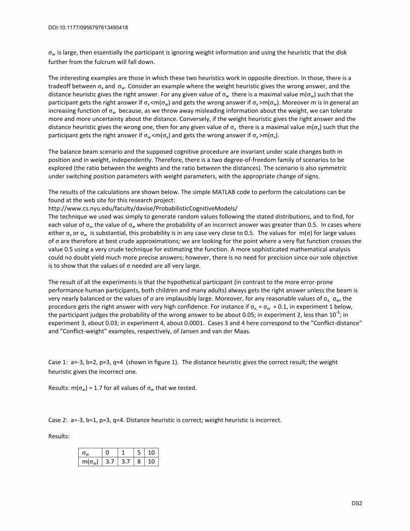
Results: m(σw) = 1.7 for all values of σw that we tested. 

 

Case 2:  a=‐3, b=1, p=3, q=4. Distance heuristic is correct; weight heuristic is incorrect. 

Results:  

σw  0  1  5  10 m(σw)  3.7  3.7  8  10 

 

DOI:10.1177/0956797613495418

DS2

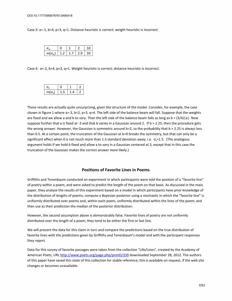
Case 3: a=‐1, b=4, p=3, q=1. Distance heuristic is correct; weight heuristic is incorrect. 

 

σw  0  1  2  10 m(σw)  1.2  1.7  2.9  10 

 

Case 4:  a=‐2, b=4, p=3, q=1. Weight heuristic is correct; distance heuristic is incorrect. 

 

σx  0  1  2 m(σx)  1.5  1.4  2 

 

These results are actually quite unsurprising, given the structure of the model. Consider, for example, the case shown in figure 1 where a=‐3, b=2, p=3, q=4. The left side of the balance beam will fall. Suppose that the weights are fixed and we allow a and b to vary. Then the left side of the balance beam falls as long as b < (3/4)|a|. Now suppose further that a is fixed at ‐3 and that b varies in a Gaussian around 2.  If b > 2.25, then the procedure gets the wrong answer. However, the Gaussian is symmetric around b=2, so the probability that b > 2.25 is always less than 0.5. At a certain point, the truncation of the Gaussian at b=0 breaks the symmetry, but that can only be a significant effect when 0 is not much more than 1.5 standard deviation away; i.e.  σx≈1.5.  (The analogous argument holds if we hold b fixed and allow a to vary in a Gaussian centered at 3, except that in this case the truncation of the Gaussian makes the correct answer more likely.)  

 

Positions of Favorite Lines in Poems. 

Griffiths and Tenenbaum conducted an experiment in which participants were told the position of a “favorite line” of poetry within a poem, and were asked to predict the length of the poem on that basis. As discussed in the main paper, they analyze the results of this experiment based on a model in which participants have prior knowledge of the distribution of lengths of poems; compute a Bayesian posterior using a stochastic in which the “favorite line” is uniformly distributed over poems and, within each poem, uniformly distributed within the lines of the poem; and then use as their prediction the median of the posterior distribution.  

However, the second assumption above is demonstrably false. Favorite lines of poetry are not uniformly distributed over the length of a poem; they tend to be either the first or last line. 

We will present the data for this claim in turn and compare the predictions based on the true distribution of favorite lines with the predictions given by Griffiths and Tenenbaum’s model and with the participant responses they report. 

Data for this survey of favorite passages were taken from the collection "Life/Lines", created by the Academy of American Poets, URL http://www.poets.org/page.php/prmID/339 downloaded September 28, 2012. The authors of this paper have saved this state of this collection for stable reference; this is available on request, if the web site changes or becomes unavailable.  

DOI:10.1177/0956797613495418

DS3

From this corpus, we extracted a data set, enumerating the poem's author and title, starting line, ending line, and length of favorite passage; and length of the poem containing the passage. This data set is available on the website associated with the study:  http://www.cs.nyu.edu/faculty/davise/ProbabilisticCognitiveModels/ 

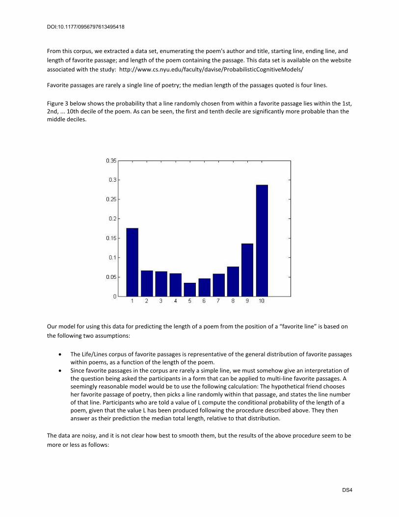
Favorite passages are rarely a single line of poetry; the median length of the passages quoted is four lines. 

Figure 3 below shows the probability that a line randomly chosen from within a favorite passage lies within the 1st, 2nd, ... 10th decile of the poem. As can be seen, the first and tenth decile are significantly more probable than the middle deciles.  

 

 

Our model for using this data for predicting the length of a poem from the position of a “favorite line” is based on the following two assumptions: 

The Life/Lines corpus of favorite passages is representative of the general distribution of favorite passages within poems, as a function of the length of the poem.  

Since favorite passages in the corpus are rarely a simple line, we must somehow give an interpretation of the question being asked the participants in a form that can be applied to multi‐line favorite passages. A seemingly reasonable model would be to use the following calculation: The hypothetical friend chooses her favorite passage of poetry, then picks a line randomly within that passage, and states the line number of that line. Participants who are told a value of L compute the conditional probability of the length of a poem, given that the value L has been produced following the procedure described above. They then answer as their prediction the median total length, relative to that distribution.  

The data are noisy, and it is not clear how best to smooth them, but the results of the above procedure seem to be more or less as follows: 

DOI:10.1177/0956797613495418

DS4

If L=1, predict 31.  If L is between 2 and 11, predict 12.  If L is between 12 and 200, predict L+2.  

The odd result on L=1 reflects the fact that there are a number of long poems for which only the first line is quoted. This statistic is probably not very robust; however, it is likely to be true that the median prediction for L=1 is indeed significantly larger than for L=2, and may even be larger than the overall median length of poem (22.5).  

The claim that, for L between 12 and 200, the prediction should L+2 is based on the following observation: There are 50 passages in which the position of the median line is greater than 12, and in 31 of those, the median line is within 2 of the end of the poem.  Thus, given that the position L of the favorite line is between 12 and 200, the probability that the poem is no longer than L+2 is much greater than 0.5. 

For L > 200, this rule probably breaks down. The last lines of very long poems do not tend to be particularly memorable. 

Comparison 

Table 2 shows the predictions of the two models and the mean participant responses at the five values L=2, 5, 12, 32, and 67 used by Griffiths and Tenenbaum in their experiment. We also show the predictions of the two models at the value L=1, since there is such a large discrepancy; Griffiths and Tenenbaum did not use this value in their experiment, so there is no value for participant responses. This comparison is shown graphically in Figure 3. The table and figure show the prediction of the number of lines that remain after the Lth line, which is the quantity actually being "predicted"; as discussed in the main paper, both of these models and any other reasonable model will predict that the poem has at least L lines. 

The numerical data for the predictions of the Griffiths and Tenenbaum model and for the participant responses were generously provided by Tom Griffiths. 

Model  L=1  L=2  L=5  L=12  L=32  L=67 Participant responses    ‐‐‐    8  10    8    8  28 Distribution of lengths  10    9    9    4   11  19 Favorite passages  30  10    7    2    2    2 

 

Table 1: Prediction of poem lengths  

DOI:10.1177/0956797613495418

DS5

 

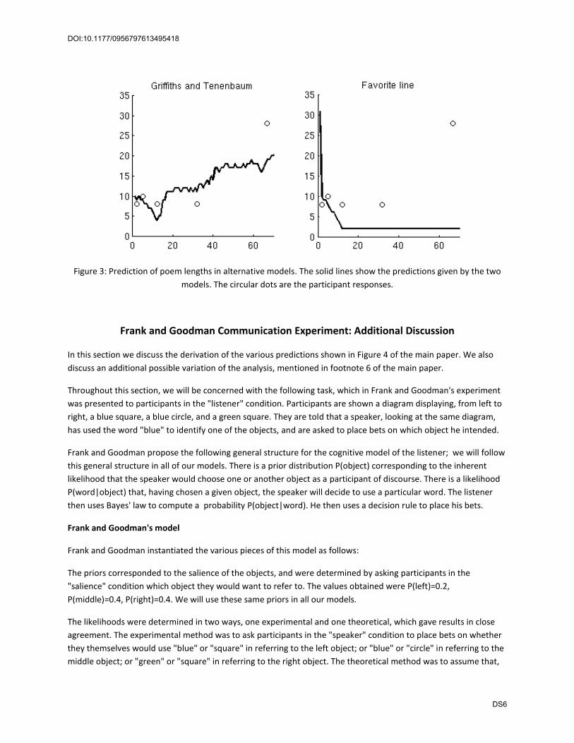
Figure 3: Prediction of poem lengths in alternative models. The solid lines show the predictions given by the two models. The circular dots are the participant responses. 

 

Frank and Goodman Communication Experiment: Additional Discussion 

In this section we discuss the derivation of the various predictions shown in Figure 4 of the main paper. We also discuss an additional possible variation of the analysis, mentioned in footnote 6 of the main paper. 

Throughout this section, we will be concerned with the following task, which in Frank and Goodman's experiment was presented to participants in the "listener" condition. Participants are shown a diagram displaying, from left to right, a blue square, a blue circle, and a green square. They are told that a speaker, looking at the same diagram, has used the word "blue" to identify one of the objects, and are asked to place bets on which object he intended. 

Frank and Goodman propose the following general structure for the cognitive model of the listener;  we will follow this general structure in all of our models. There is a prior distribution P(object) corresponding to the inherent likelihood that the speaker would choose one or another object as a participant of discourse. There is a likelihood P(word|object) that, having chosen a given object, the speaker will decide to use a particular word. The listener then uses Bayes' law to compute a  probability P(object|word). He then uses a decision rule to place his bets. 

Frank and Goodman's model 

Frank and Goodman instantiated the various pieces of this model as follows: 

The priors corresponded to the salience of the objects, and were determined by asking participants in the "salience" condition which object they would want to refer to. The values obtained were P(left)=0.2, P(middle)=0.4, P(right)=0.4. We will use these same priors in all our models.  

The likelihoods were determined in two ways, one experimental and one theoretical, which gave results in close agreement. The experimental method was to ask participants in the "speaker" condition to place bets on whether they themselves would use "blue" or "square" in referring to the left object; or "blue" or "circle" in referring to the middle object; or "green" or "square" in referring to the right object. The theoretical method was to assume that, 

DOI:10.1177/0956797613495418

DS6

for any given object O, the probability that a speaker will use word W to refer to O is proportional to the utility of that choices, which is proportional to the specificity of W for O, where the specificity is the reciprocal of the number of objects in the scenario that W describe. The words "blue" and "square" each refer to two objects; the words "green" and "circle" each refer to one. Therefore the specificity of "blue" for the left or middle object is 1/2; the specificity of "square" for the left or right object is 1/2; the specificity of "circle" for the middle object and of "green" for the right object is 1. Therefore the likelihoods for "blue" are: P("blue"|left) = 0.5/(0.5+0.5) = 0.5; P("blue"|middle)=0.5/(1+0.5) = 0.333. Of course P("blue"|right) = 0.  

Applying Bayes' law, the posterior probabilities, given that the speaker has said "blue", are 

P(left|"blue") = P("blue"|left)*P(left) / (P("blue"|left)*P(left) + P("blue"|middle)*P(middle)) = (0.5*0.2)/(0.5*0.2+0.333*0.4)  = 0.43 

P(middle|"blue") = P("blue"|middle)*P(middle) / (P("blue"|left)*P(left) + P("blue"|middle)*P(middle)) = (0.333*0.4)/(0.5*0.2+0.333*0.4)  = 0.57 

Finally,  Frank  and  Goodman  assumed  that  participants  would  split  their  bets  proportional  to  the  posterior probability; thus they split their bets 43:57:0. This agreed well with the their experimental data. 

Alternative decision rules 

If participants' reasoning is carried out using the rule that agents follow the maximum expected utility (MEU)  rule, then the results of the reasoning are very different. The MEU rule states that an agent should always choose the action  with  the  greatest  expected  utility;  it  is  universally  considered  normatively  correct.1  Either  placing  bets proportionally  to  the  probability  of  an  outcome,  or  choosing  actions  with  a  probability  proportional  to  their expected utility, is a suboptimal strategy. Frank and Goodman's calculation of the likelihoods, above, is based on the assumption that  the  listener assumes that  the speaker  is  following the second of  these suboptimal  strategy, choosing with probability 2/3 to use "circle" to refer to the blue circle, rather than doing so with probability 1, as the MEU  rule  would  prescribe.  Their  calculation  of  the  bets  placed  by  the  listeners  assumes  that  the  listeners themselves are following the first of these suboptimal strategies, hedging their bets, rather than placing all their money on the more likely outcome, which is what the MEU rule would prescribe. 

There are thus four possibilities: 

1. The listener believes that the speaker will choose his word proportionally, and the hearer splits his bet. This is the model adopted by Frank and Goldman. 

2. The hearer believes that the speaker will choose his word proportionally, and the hearer, following MEU, places all his money on the more likely posterior probability. 

3. The hearer believes  that  the  speaker will definitely  choose  the more  informative word,  following MEU, but the hearer himself splits his bet. 

4. The hearer believes that the speaker will follow MEU, and he himself follows MEU. In a theory that posits that agents are rational, this is surely the most appropriate of the options. 

Possibilities (3) and (4) actually have the same outcome. If the speaker follows MEU, then the probability that he will refer to the middle object as "blue" is 0, since he has the option of referring to it as "circle". Hence, applying Bayes' rule, 

                                                           1 The normatively proper method of using bets to elicit subjective probabilities, following de Finetti,  is to ask participants at what odds they would take one side or another of a bet (see (Russell and Norvig 2010) 489‐490). 

DOI:10.1177/0956797613495418

DS7

P(left|"blue") = P("blue"|left)*P(left) / (P("blue"|left)*P(left) + P("blue"|middle)*P(middle)) = (0.5*0.2)/(0.5*0.2+0*0.4)  = 1.0 

P(middle|"blue") = P("blue"|middle)*P(middle) / (P("blue"|left)*P(left) + P("blue"|middle)*P(middle)) = (0*0.4)/(0.5*0.2+0*0.4)  = 0 

Since there is no probability that the speaker will describe the middle object as "blue", if he uses the word "blue", it is entirely certain that he means the left object. Therefore, whether the listener is following MEU or hedging his bets, he should put all his money on the left object. 

In possibility (2), the posterior probabilities will be the same as in Frank and Goodman's calculation above: P(left|"blue") = 0.43, P(middle|"blue") = 0.57. However, the listener, following MEU, should place all his money on the more likely outcome, which is the middle object. 

Choice of words 

All  of  the  above  calculations  are  based  on  the  assumption  that  the  listener  is  aware  that  the  only  four  words available for the speaker are "blue", "green", "square", and "circle". However, this information is not given to the listener in the experimental setup described, and it  is by no means clear how he comes to this awareness. There are certainly other single words that could be used by the speaker; either synonyms or near synonyms for these such as "turquoise", "emerald", "rectangular", and "round"; words referring to positions such as  "left", "middle" and "right"; and other words, such as “shape”, “picture”, or “salient”.  If the space of words were increased then that would certainly change the theoretical calculation of the specificity of these words, and it might well change the behavior of the participants in the "speaker" condition. 

Suppose,  for  instance,  that  the  space  of words  under  consideration  is  expanded  to  include  "round", which  has specificity 1 with  respect  to  the middle object.  If we  follow Frank and Goodman's model  in assuming  that both speaker  and  hearer  follow  suboptimal  decision  rules,  the  calculation  proceeds  as  follows:  The  likelihood P("blue"|left)  =  0.5  as  before.  The  likelihood  P("blue"|middle)  =    0.5/(0.5+1+1)  =  0.2.  Applying  Bayes'  law,  we obtain the posteriors 

P(left|"blue") = P("blue"|left)*P(left) / (P("blue"|left)*P(left) + P("blue"|middle)*P(middle)) = (0.5*0.2)/(0.5*0.2+0.2*0.4)  = .55 

P(middle|"blue") = P("blue"|middle)*P(middle) / (P("blue"|left)*P(left) + P("blue"|middle)*P(middle)) = (0.2*0.4)/(0.5*0.2+0.2*0.4)  = .45 

The two posterior probabilities have thus switched places. Now, of course, the decision just to add the word "round" was entirely arbitrary, but so was the original set of words.2 The reader may enjoy calculating the effect of this extension on the alternative models. 

Gweon, Tenenbaum, and Schulz experiment on infants' reasoning about samples 

The paper discussed in this section came to our notice too late to include a discussion in the main paper; however since it vividly illustrates the kinds of arbitrary assumptions that can be made in the application of Bayesian models, we have included it here, in this supplement.                                                            2 One principled approach to this issue would be to use all possible adjectives and nouns that could apply to these objects among the thousand most common words in English. In that case, the question would arise how the frequency of these words should be combined with the specificity measures proposed by Frank and Goodman in computing the overall prior. We have not carried out this calculation. 

DOI:10.1177/0956797613495418

DS8

Gweon, Tenenbaum, and Schulz (2011) carried out the following experiment: 15 month old infants were shown a box containing blue balls and yellow balls. In one condition of the experiment, 3/4 of the balls were blue; in the other condition, 3/4 were yellow. In both conditions, the experimenter took out three blue balls in sequence, and demonstrated that all three balls squeaked when squeezed. The experimenter then took out an inert yellow ball, and handed it to the baby. The experimental finding was that, in condition 1, 80% of the babies squeeze the yellow ball to try to make it squeak, whereas in condition 2, only 33% of the babies squeeze the ball. 

The explanation of this finding given by Gweon, Tenenbaum, and Schulz is as follows. The babies are considering two possible hypotheses about the relation of color to squeakiness: Hypothesis A is that all balls squeak; hypothesis B is that all and only blue balls squeak; (the obvious third alternative  that only yellow balls squeak is ruled out by the observation, and therefore can be ignored). Thus if A is true, then the yellow ball will squeak; if B is true, it will not. The babies are also considering two possible hypotheses about the experimenter's selection rule for the first three balls. Hypothesis C is that the experimenter is picking at random from the set of all balls; hypothesis D is that she is picking at random from the set of all balls that squeak,  

The intuitive explanation then, is this. If most of the balls in the box are blue, then the fact that the experimenter has pulled three blue balls is unsurprising, and thus reveals nothing about her selection strategy. If most of the balls are yellow, however, then that suggests that she is pursuing a particular selection strategy to extract the three blue balls. That selection strategy must be selecting balls that squeak, since that is the only selection strategy under consideration. Then the fact that selecting balls that squeak gives all blue balls suggests that only the blue balls squeak. 

We can formalize this argument as follows: Let z be the fraction of blue balls in the box. Let p=Prob(A), q=Prob(C), so Prob(B) = 1―p and Prob(D) = 1―q. Assume that A vs. B is independent of C vs. D and that they are both independent of z. Let S be the event that the experimenter selects three blue balls (note that under either hypotheses A or B, the blue balls will all squeak). Then the baby can calculate the probability of A given the observation of the three squeaky blue balls as follows. 

Prob(S|A,z) = z3 

Prob(S|B,C,z) = z3 

Prob(S|B,D,z) = 1 

    Therefore 

             Prob(S|z) = pz3 + (1―p)qz3 +(1―p)(1―q) 

Prob(A,S|z) = pz3 

 So Prob(A|S,z) = Prob(A,S)/Prob(S) = pz3 / (pz3 + (1―p)qz3 +(1―p)(1―q)) 

It is easily seen that this is an increasing function of z; for instance as z goes to 0, this fraction goes to 0; as z goes to 1, the denominator approaches 1, so the fraction converges to p. If we choose p=q=1/2, then Prob(A|S,z=3/4) = 0.37, whereas Prob(A|S,z=1/4) = 0.03. 

Thus, if most of the balls in the box are blue (z=3/4), there is a reasonable chance (though less than ½) that all balls squeak; if most of the balls in the box are yellow (z=1/4), it is extremely likely that only blue balls squeak. 

DOI:10.1177/0956797613495418

DS9

There are many difficulties here. The most obvious is that the choice of strategies is limited to C and D. Another obvious alternative is (E) that the experimenter is deliberately selecting only blue balls.  A priori this would seem more likely than D, since the experimenter can easily see which balls are blue, but cannot see which balls squeak, If one adds this to the model as a third possibility, then Prob (A|S,z) is still an increasing function of z, but the dependence is much weaker. 

We can redo the calculation as follows. Let q=Prob(C), r=Prob(D), so Prob(E) = 1―(q+r). We have now 

Prob(S|A,C) = z3 

Prob(S|A,D) = z3 

Prob(S|A,E) = 1 

Prob(S|B,C) = z3 

Prob(S|B,D) = 1 

Prob(S|B,E) = 1 

    Therefore 

             Prob(S) = (q+pr)z3 + 1 – q ‐ pr 

Prob(A,S) = p(q+r)z3 +  p(1―(q+r)) 

 So Prob(A|S) = Prob(A,S)/Prob(S) = (p(q+r)z3 +  p(1―(q+r)))/ ((q+pr)z3 + (1―p)r + (1―(q+r))) 

If we choose p=1/2, q=r=1/3 then the results are 

Prob(A|S,z=3/4) = 0.43 

Prob(A|S,z=1/4) = 0.34 

The babies are thus making a quite strong distinction on the basis of a fairly small difference in posterior probability. 

If we take into account that D is inherently less plausible than E, then the difference becomes even smaller. Suppose for instance that C and E are equally plausible and that D is half as plausible as either; thus q=2/5, r = 1/5. Then 

Prob(A|S,z=3/4) = 0.46 

Prob(A|S,z=1/4) = 0.40 

As r goes to zero, the dependence of the posterior probability of A on z also vanishes. 

Another problem is the assumption that the selection strategy applies only to the first three blue balls. If the strategy is "Select balls that squeak" and the experimenter is pursuing this strategy in choosing the yellow ball as well, then the probability is 1 that the yellow ball will squeak. It is hard to see why the baby should assign probability 0 to this interpretation of what the experimenter is doing. Gweon, Tenenbaum, and Schulz address this possibility in a footnote as follows: 

DOI:10.1177/0956797613495418

DS10

The model mirrors the task design in distinguishing the sampling phase from the test phase. Because the yellow ball was treated differently from the blue ball(s) (i.e. given directly to the children and not manipulated by the experimenter), we do not treat the yellow ball as part of the sample in the model. 

But how do they know that the baby takes the same view of the matter? Alternatively, the baby might reason that, since the experimenter didn't bother to squeeze the yellow ball, it must not squeak.  

One can also question the independence of A and B from z. An optimistic baby might reason that, after all, a box should contain a lot of squeaky balls; therefore if a box contains a lot of yellow balls, that in itself suggests that yellow balls should squeak.  A pessimistic baby might make the reverse argument. 

 Another difficulty is that equating the fraction of babies who think that the ball will squeak with the probability that any given baby thinks that the ball will squeak is hard to justify. Each individual baby, after all, either does or does not squeeze the ball; if babies are all perfectly rational, all have the same priors, and the same decision rule (e.g.  squeeze the ball if the a posteriori probability that it will squeak is greater than 1/3) then under any given circumstance, they should either all squeeze the ball or all not squeeze the ball. There are a number of possible answers here; they may have different priors on the hypotheses, or they may assign different ratios of the utility of getting a squeak vs. the disutility of making the effort to squeeze the ball. But even so, the translation of the probability into cross‐participant action frequency is tricky.  

Gergely and Jacob (2013) propose an alternative explanation of these results, resting on the idea, which has independent experimental evidence, that infants distinguish between instrumental and communicative actions in people who are interacting with them (in this case the experimenter).  However, their analysis relies on the same anomalous choice of the selection criterion under consideration, and therefore is subject to the same critique. 

References 

Gergely, G. & Jacob, P. (2013). Reasoning about instrumental and communicative agency in human infancy. In F. Xu and T. Kushnir (eds.) Rational Constructivism in Cognitive Development, Amsterdam:Elsevier, 59‐94.  Jansen, B. R. J., & van der Maas, H. L. J. (1997). Statistical test of the rule assessment methodology by latent class analysis. Developmental Review, 17, 321–357.  

Russell, S. and Norvig, P. (2010) Artificial Intelligence: A Modern Approach. 3rd edn., Prentice Hall.   

 

DOI:10.1177/0956797613495418

DS11